Working paper

Food crop production in Tanzania

Evidence from the 2008/09 National Panel Survey

Vincent Leyaro Basile Boulay Oliver Morrissey

December 2014 When citing this paper, please use the title and the followingreference number:F-40110-TZA-1

Food crop production in Tanzania: Evidence from the

2008/09 National Panel Survey

Research report to IGC Tanzania

Vincent Leyaro

Department of Economics, University of Dar-es-Salaam

Oliver Morrissey and Basile Boulay

School of Economics, University of Nottingham

December, 2014

Abstract

An earlier scoping study showed that the Tanzania National Panel Surveys (NPS) of 2008/09

and 2010/11 provide useable data to address productivity and supply response in agriculture.

This report provides analysis of long season food crops for the first wave of the NPS

(2008/09) concentrating on supply response, the price and non-price factors determining

production and how responsive farmers are to these factors. The report highlights important

limitations in the NPS data for analysis of supply response, notably the absence of market

prices and that few farmers report using purchased inputs. Nevertheless, we identify certain

core determinants of production and show that farmers are responsive to prices.

Contents

1. Context: Agriculture in Tanzania

2. Data Measurement and Issues

3. Empirical Methodology

4. Econometric Results

5. Conclusions

References

Appendices

JEL Classifications: Keywords: Agricultural Productivity, Supply Response, Panel Surveys, Tanzania

2

1 Context: Agriculture in Tanzania

After 50 years of independence, despite apparent commitment to policies and strategies to

transform the agriculture sector, performance in agricultural output and productivity has been

disappointing. Policies and plans, such as ‘agriculture is the mainstay of the economy’ and

Kilimo Kwanza (agriculture first), have remained slogans to the public as there is so little

experience of reforms that have improved livelihoods and millions in the agriculture sector

remain in poverty. Tanzania is endowed with considerable fertile agricultural land and inland

fresh water resources that can be utilized for irrigation, but much of the land is underutilized

and what is utilised often exhibits very low productivity. In this sense Tanzania has yet to

achieve the traditional ‘structural transformation’ whereby increasing agricultural production

provides a platform for manufacturing and economic growth. Balanced growth is achieved if

agriculture becomes increasingly commercialized while the manufacturing sector grows.

Initially manufacturing may be based on agriculture, through processing and agri-business,

but ultimately manufacturing and the economy will become diversified. This has not

happened in Tanzania, and the economy remains essentially agriculture-based, mostly a

peasant economy with low productivity. Understanding the factors that can expand

production and enhance agricultural productivity in Tanzania is critical for ensuring

‘structural transformation’ and economic growth, boosting development and reducing poverty

(given that the majority of the poor are in rural areas and in agricultural activities).

Although the contribution of agriculture sector to GDP and exports earnings has been

falling over time, to around 25 percent of GDP and 20 percent of export earnings in 2012

compared to where it was in 1970s and 1980s where the sector accounted for more than 50

per cent of GDP and 75 per cent of export earnings; the sector remains important as some 80

per cent of Tanzanians depend on agriculture for their livelihood and 95 percent of their food.

Consequently, the National Development Vision 2025, the main national development

strategy in Tanzania, places considerable emphasis on the sector and envisages that by 2025

the economy will have been transformed from a low productivity agricultural economy to a

semi-industrialized one led by modernized and highly productive agricultural activities that

are integrated with industrial and service activities in urban and rural areas. Against this

background, in the last decade a number of polices and strategies have been formulated to

support agriculture in a more systematic way. The Agricultural Sector Development Strategy

(ASDS) was adopted in 2001, and gave rise to the Agricultural Sector Development Program

(ASDP) of 2005; and the Cooperative Development Policy (CDP) of 2002, complemented by

3

a variety of sector policies. The strategy and the ASDP are embedded in the National Strategy

for Growth and Reduction of Poverty (NSGRP), which is a medium term plan to realize

Vision 2025. Kilimo Kwanza (agriculture first), developed in 2009, provides additional inputs

for the implementation of ASDP and other programs favourable for the agricultural sector. It

is an assertion of the commitment of the government and the private sector to agricultural

development, and it invites all Tanzanians to become part of this commitment. Its ten pillars

support the ASDS and the ASDP and strengthen them by adding additional initiatives, in

particular in rural finance.

The agriculture sector is therefore seen as a main vehicle in any national economic

strategy to combat poverty, enhanced agricultural productivity is crucial to realize the

objectives, and the policy statements have at least identified the issues and proposed a

strategy. The ASDS emphasized the need to improve the efficiency of input markets and

product marketing, increase access to credit, enhance the provision of extension services and

increase investment in rural areas (especially for irrigation and transport). The ASDP was in

principle the strategy to implement these aims, but had limited impact – the strategies were

not a success. Thus, the culmination of these initiatives was the formulation of a belief in the

need to ‘reintroduce selective subsidies, particularly for agricultural inputs, machinery and

livestock development inputs and services’ (ESRF, 2005: xii). Thus, by providing some

quantitative assessment of the importance of different factors (such as prices, access to credit

and other inputs, access to markets and marketing) to output levels for the major crops, this

research contributes to understanding why the strategy has failed and providing

recommendations of factors to target for an effective strategy.

Despite the CDP, the cooperative sector has failed to respond to the challenge of

liberalization. The sector suffers from weak managerial (and advocacy) skills, a lack of

financial resources (in particular undercapitalization of cooperative banks, so credit

constraints remain), and a weak institutional structure (especially in that they are not

accountable to members). Thus, although the cooperative sector remains significant it is not

viewed as successful, either in supporting development and growth or in representing the

interests of members, giving added impetus to liberalization initiatives.

Agriculture is recognized as integral to the Poverty Reduction Strategy, and

agricultural sector growth is essential if Tanzania is to achieve sustained economic

development. While this may seem somewhat obvious, it marks a change in emphasis – the

whole sector (not only export crops) has attained a higher status on the policy (and political)

4

agenda, and a view is emerging that there is a need for positive support to the sector. In this

context, it is timely to attempt to assess the determinants of production and productivity in

agriculture using crop and farm level data.

Although there have been many studies of agriculture in Tanzania, there are no recent

nationwide studies of production and productivity covering all major crops. As part of the

World Bank project on Distortions to Agriculture in Africa (Anderson and Masters, 2009),

Morrissey and Leyaro (2009) provided an analysis and discussion of the bias in agriculture

policy in Tanzania over the period 1976-2004. They found that reforms implemented since

the late 1980s have reduced distortions in agriculture, but certain crops (especially cash

crops) have become less competitive due to serious deficiencies in marketing and

productivity. The level of distortion against agriculture remained reasonably high for all cash

crops up to the early 2000s. Analysing time series data over 1964-1990, McKay et al (1999)

find that food crop production increased as prices increases relative to export crops, implying

aggregate export crop production was not responsive to prices. As producers seem to respond

to the relative price and incentives for food crops compared to cash crops, with high relative

price elasticity for food crops (McKay et al, 1999), one expects increasing food production in

the latter half of the 2000s.

Arndt et al (2012) use representative climate projections in calibrated crop models to

estimate the impact of climate change on food security (represented by crop yield changes)

for 110 districts in Tanzania. Treating domestic agricultural production as the channel of

impact, climate change is likely to have an adverse effect on food security, albeit with a high

degree of diversity of outcomes (including some favourable). Ahmed et al (2012) identify

the potential for Tanzania to increase its maize exports as climate change scenarios suggest a

decline in maize production in major exporting regions. Specifically, climate predictions

suggest that some of Tanzania's trading partners will experience severe dry conditions in

years when Tanzania is only mildly affected. Tanzanian maize production is far less variable

than that of major global producers (no significant growth, but no large declines due to

weather shocks), including compared to other SSA producers (Ahmed et al, 2012, p 403), so

has scope to respond to the adversity other producers will face. However, as shown by Arndt

et al (2012), Tanzania may itself suffer a decline in production. Addressing the reasons why

production in Tanzania has not grown is crucial to create a production environment within

which productivity can increase, and maize is a crop worthy of specific attention.

5

The next section discusses the basic data used in the estimation, and Section 3 presents

the empirical strategy. Section 4 presents and discusses the results, with conclusions in

Section 5 that tease some policy implications.

2 Data measurement and definitions

The National Panel Surveys (NPS) are a series of nationally representative household panel

surveys that assemble information on a wide range of topics including agricultural

production, non-farm income generating activities, consumption expenditures and socio-

economic characteristics. The 2008/09 NPS is the first in the series conducted over twelve

months, from October 2008 to October 2009, implemented by the Tanzania National Bureau

of Statistics (NBS) with a sample based on the National Master Sample frame, largely a sub-

sample of households interviewed for the 2006/07 Household Budget Survey.

The 2008/09 NPS covered 3,280 households from 410 Enumeration Areas (2,064

households in rural areas and 1,216 in urban areas). The agriculture production data are

collected and reported by plot (j) for household (i) and crop (c), recording inter-cropping and

allowing for the long and short seasons crops, and perennial (tree) crops.1 Most variables

have to be calculated at the plot level as although over 40 per cent of households have only

one plot and fewer than 10 per cent have more than three plots, most plots are used to grow

more than one crop either by inter-cropping or sub-dividing the plot. Plot-level data are

calculated and aggregated up to the farm (household) level. For the detailed descriptive

statistics at the farm-level (mean and median) by crop and agro-ecological zones (or region)

to capture the distribution of farm size and of products and inputs prices across farms see the

scoping study (Leyaro and Morrissey, 2013).

The data we use in this study is the first wave (2008/09) of the NPS. Except for the

number of working adults per household (obtained from the Household questionnaire), all

data were obtained from the Agricultural questionnaire. The original sample consists of 3280

households but our final sample size is significantly smaller, due to missing data and

exclusion of outliers following graphical and statistical analysis. Further, we focus on annual

crops (thus omitting important crops such as coffee) and rely on data for the long rainy

1 Long season crops data file is appended on top of short season crops data file for the same variables and this

new data file is then appended on top of perennial (tree) crops file for the same variables. Variables are then

aggregated at farm (household) level for descriptive analysis and estimation.

6

season only. When referring to ‘total harvest’, or ‘total production’, we thus refer to total

values for annual crops for the long season. We have in total 1670 households in our sample.

Since we are using only one wave we show that there is enough variation in prices at the

farm level to allow for analysis (see Leyaro and Morrissey, 2013). Our analysis aims at

understanding what drives supply response in agriculture at the aggregate level. Therefore,

total harvest (in Kg) and total value of sales will be our main dependent variables, as well as

quantities of variable inputs demanded. Variable inputs considered are total hired labour

(defined as the sum of men and women labour days hired for land preparation, weeding, and

harvesting), and chemical (inorganic) fertiliser used (in Kg). Those can be treated as variable

inputs rather than quasi-fixed inputs, as in Hattink et al (1998), since we have data on wage

bills and expenditures on chemical fertiliser. Note that variable inputs use is given at the plot

level, that is, it refers to the total harvest realised on that plot, rather than the amount of that

harvest which is then sold. Therefore, such variables are only suitable when using harvest as

the dependent variable. When using quantity sold as the dependent variable (i.e., a fraction of

harvest), we use a weighted version of those variable inputs regressors (weighted by the

proportion of the harvest which is actually sold). Not doing so would yield upward biased

results for variable input use. Variable input prices are also calculated (daily wage rate and

price per kilogram of chemical fertiliser) by dividing total amount hired/used by total

expenditure. They are then divided by unit price to normalise them, following the standard

approach in the literature. Unit prices are derived by dividing total sales (in Tanzanian

shillings) by total quantity sold. Most studies considering total value of sales or total output

supplied onto the market as dependent variables would generally normalise them using a

market price index, as in Abrar et al (2004a). However, in this case, there is no market price

index available, so that no normalisation is made in regressions using total output sold as the

dependent variable.

Quantity of organic fertiliser used (in Kg) is considered as a fixed input, and is a proxy for

animal power, usually defined as the number of oxen owned, which was not directly

available. Following Abrar el al (2004a), organic fertiliser may be seen as capturing a wealth

effect. Family labour is also considered as a fixed input, and is defined as the total number of

working-age adults (15 to 65 years old inclusive) per farm. Control variables included are

total area cultivated (in acres) and average distance to nearest village market (in Km). A

`weighted’ version of the distance variable is used, where distance is weighted by area.

Weighted average distance may be used instead of average distance for greater accuracy as it

7

may capture interactions between land size and distance to the market. Finally, weighted

property (the percentage of land cultivated which is owned by the farm/household) is also

considered as a control variable in order to capture property rights or incentive effects. We

will use these weighted variables throughout and simply refer to them as Distance and

Property for convenience.

As around 85% of farms in the sample make no use of chemical fertilizer, and around 60%

do not hire labour, it is likely that summary statistics for the whole sample are not very

informative. We therefore consider four sub-samples: Group 1, the 836 households not using

any variable input; Group 2, the 588 households hiring labour only; Group 3, the 107

households buying chemical fertilizer only; and Group 4, the 139 households buying both

variable inputs. Thus, about 50% of the total sample does not use any variable inputs, whilst

only 8% uses both.

Table 1: Summary statistics for sample and groups

Whole sample Group 1 Group 2 Group 3 Group 4

Observations 1670 836 588 107 139

Harvest (Kg) 1058 771 1281 1344 1618

Quantity sold (Kg) 315 161 426 407 698

Marketed surplus (%) 30 21 33 30 43

Sales (TSh) 113769 53378 137946 207982 302187

Unit price (TSh) 231 190 245 342 343

Organic fert. (Kg) 171 51 219 305 579

Adults 2.77 2.80 2.73 2.76 2.81

Area 3.99 3.44 4.62 3.76 4.80

Distance 4.94 5.22 4.84 4.10 4.33

Property 0.57 0.62 0.54 0.43 0.49

Inorganic fertilizer (Kg) 15.6 106 106

Inorganic (weighted, Kg) 5.4 28.8 42.7

Fertilizer price 0.40 2.67 2.72

Labour (days) 11.9 26.7 29.32

Labour (weighted, days) 3.95 8.03 13.46

Wage rate 3.32 7.10 9.78

Source: Author’s own construction based on 2008/09 NPS

8

Figure 1: Variation in unit prices

Source: Author’s own construction based on 2008/09 NPS

Table 1 provides summary statistics for the whole sample and the four groups. Mean

values are reported as well as respective sample size (standard deviations are not reported).

We also include for convenience the percentage of marketed surplus for each group (quantity

sold divided by harvest). A general analysis of agricultural supply response using the whole

sample is inappropriate as most households do not purchase any variable input so each group

warrants separate statistical treatment. Farms in Group 1 have the lowest average harvest and

sales at the lowest unit price, just over half the unit price achieved by the higher producing

farms in Groups 3 and 4. There is considerable variation in unit prices across the sample;

although almost 90% of prices are around 500 Tanzanian Shillings or less, there is a

noticeable skew to the right (Figure 1).

Marketed surplus is only 21% for Group 1, suggesting widespread subsistence farming

and sharply contrasting with Group 4 with a marketed surplus of 43%. There is also variation

in variable input use and the proportion of non-users of chemical fertilizer and that of non-

users of hired labour is particularly high. The disaggregated picture reveals interesting

features. In particular, the difference in production variables between Groups 1 and 4 is

striking, which confirms our intuition that subsistence farming may be widespread in Group

1, together with a lower degree of market integration than in Group 4. Apart from the fact

9

that both harvest and quantity sold are much greater in Group 4 than in Group 1, it is clear

that the proportion of harvest that is marketed is also much greater in Group 4.

While the differences between Groups 3 and 4 are fairly small (except for quantity

harvested and sold and organic fertilizer use), Groups 1 and 2 look quite different to Group 4.

As expected, average use of organic fertilizer (which may capture a wealth effect) is

extremely low in Group 1, in which farmers do not buy any variable inputs, possibly due to

financial constraints. Farmers in Group 4 use 11 times as much organic fertilizer as their

counterparts from Group 1. The difference is also very marked with Groups 2 and 3,

suggesting that constraints faced by farmers in Group 1 may not be faced by those using one

variable input only, or at least, not faced with the same intensity. Regarding family labour,

the average is very close across groups, while the average total area cultivated is significantly

higher in Group 4 than in Group 1. The smallest farms in the sample are located in Group 1,

but these have the highest weighted property index with an average of 62% of total area

cultivated owned, as opposed to 49% in Group 4.

3 Empirical methodology

Although the NPS are small in sample size (3,280 households), they provide recent farm level

household panel data for which econometric analysis is feasible. The analysis presented

addresses supply response, the price and non-price factors determining production and how

responsive farmers are to these factors. Two fundamental approaches are used in studying

production decisions: the production function (primal approach) and the profit function (dual

approach). Under appropriate regularity conditions, and with the assumption of profit

maximization, both functions contain the same essential information on a production

technology. The dual approach has several advantages: prices are specified as the exogenous

variables as opposed to input quantities (prices are usually less collinear than input

quantities); estimates of output supply, input demand, and the price (and cross-price)

elasticities are more easily derived (as derivatives of the profit function); and it is more

flexible for modelling multiple outputs and inputs systems (as is the case here).

Following Abrar et al. (2004a) a profit, cost, or revenue function is estimated

employing a variant specification of the profit function. Assume that farmers attempt to

maximise restricted profit, defined as the return to the variable factors, so the profit

maximisation problem can be expressed as:

10

Max Π (p,w;z) = Ma x p'y – r'x (1)

s.t. F(y, x; z) ≤ 0,

where Π , p, w, respectively, represent restricted profit, and vectors of output and

input prices. The variables y and x represent vector of output and input quantities

respectively. F(.) is the production technology set of the producer, and Z is a set of control

variables. The restricted profit function represents the maximum profit the farmer could

obtain with available prices, fixed factors, and production technology. The profit-maximising

output supply and input demand functions are derived as:

m

mP

zwpzwpY

;,);,( , ,,...,1 Mm (2)

and

n

nW

zwpzwpX

;,);,( , .,...,1 Nn (3)

where m and n index the outputs and variable inputs respectively. There are usually

four (translog, generalised Leontief, generalised Cobb-Douglas, and the quadratic forms)

functional forms of the profit function that have been used in the literature. A choice of a

particular specification, in part, depends on the nature of the data set available. The translog

profit function is generally preferred if the level of analysis includes a number of crops (i.e.

farms are treated as multi-product producers). As we are using an aggregate of food crop

production, a Cobb-Douglas production is appropriate.

Due to the nature of the data, and in particular, the very large proportion of farms that

do not use any variable inputs, our modelling strategy has two parts. We firstly focus on those

farms not buying any variable inputs. A full study of supply response in this context seems

inappropriate since those farms may be characterized by subsistence farming and low market

integration (in essence, such households may not satisfy assumptions underlying the

estimation of a restricted profit function). We will therefore do some preliminary exploratory

analysis on this sub-sample. We then consider a more complete analysis of production and

supply behaviour using data of farms using at least one variable input.

11

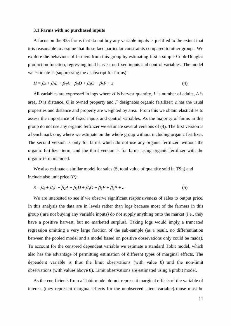
3.1 Farms with no purchased inputs

A focus on the 835 farms that do not buy any variable inputs is justified to the extent that

it is reasonable to assume that these face particular constraints compared to other groups. We

explore the behaviour of farmers from this group by estimating first a simple Cobb-Douglas

production function, regressing total harvest on fixed inputs and control variables. The model

we estimate is (suppressing the i subscript for farms):

H = 0 + 1L + 2A + 3D + 4O + 5F + (4)

All variables are expressed in logs where H is harvest quantity, L is number of adults, A is

area, D is distance, O is owned property and F designates organic fertilizer; has the usual

properties and distance and property are weighted by area. From this we obtain elasticities to

assess the importance of fixed inputs and control variables. As the majority of farms in this

group do not use any organic fertilizer we estimate several versions of (4). The first version is

a benchmark one, where we estimate on the whole group without including organic fertilizer.

The second version is only for farms which do not use any organic fertilizer, without the

organic fertilizer term, and the third version is for farms using organic fertilizer with the

organic term included.

We also estimate a similar model for sales (S, total value of quantity sold in TSh) and

include also unit price (P):

S = 0 + 1L + 2A + 3D + 4O + 5F + 6P + (5)

We are interested to see if we observe significant responsiveness of sales to output price.

In this analysis the data are in levels rather than logs because most of the farmers in this

group ( are not buying any variable inputs) do not supply anything onto the market (i.e., they

have a positive harvest, but no marketed surplus). Taking logs would imply a truncated

regression omitting a very large fraction of the sub-sample (as a result, no differentiation

between the pooled model and a model based on positive observations only could be made).

To account for the censored dependent variable we estimate a standard Tobit model, which

also has the advantage of permitting estimation of different types of marginal effects. The

dependent variable is thus the limit observations (with value 0) and the non-limit

observations (with values above 0). Limit observations are estimated using a probit model.

As the coefficients from a Tobit model do not represent marginal effects of the variable of

interest (they represent marginal effects for the unobserved latent variable) those must be

12

computed separately; we use a maximum likelihood (ML) estimator. Average marginal

effects conditional on positive sales can then be computed using the inverse Mills Ratio. We

also compute average marginal effects of price as total area cultivated varies (to see whether

the ‘price factor’ becomes more important as more land is cultivated, which we expect), and

as the quantity of organic fertilizer used varies (which we expect to be increasing reflecting

more wealth and market integration).

3.2 Farms with purchased inputs

A different estimation strategy is appropriate for those farms that purchase at least one

variable input; farms for which both hired labour and purchased fertilizer is zero are

excluded. The approach used is to estimate a restricted profit function derived as total sales

(total value of output sold) minus cost of variable inputs following Abrar et al (2004a,

2004b), Hattink et al (1998) and Savadogo et al (1995) by using a quadratic functional form.

The basic underlying assumptions are that farmers intend to maximise restricted profits and

that markets are competitive. This method is rooted in the dual approach to estimating a profit

function rather that the production function directly, as outlined in (1) – (3) above. In essence,

information about production and technology can be recovered from the profit function,

provided the assumptions of competitive markets and profit maximising behaviour are

satisfied. The 18 farms with negative restricted profit are omitted, following Abrar et al

(2004b). The quadratic normalised profit function generates specifications of (2) and (3) to be

estimated using the quantity of marketed output and quantities of purchased and fixed inputs.

Following the standard approach, these are estimated using iterative seemingly unrelated

regressions (SUR) with bootstrap standard errors.

Complications arise given the extremely large proportion of farms that do not appear to

devote fertilizer to that part of the harvest which is marketed, as well as the large proportion

that do not hire labour. This creates ‘censored data’, which, if not accounted for, will bias

results. Standard OLS technique will fail to account for the non-linearity in the data, and will

also fail to account for the qualitative difference between censored and non-censored

observations. We follow the approach of Hattink et al (1998) and Abrar et al (2004b) to

address this problem, using a Heckman 2-step estimator by first estimating a Probit model on

all observations, deriving the inverse Mills Ratios and using these as additional regressors in

the second stage OLS regression using those observations for which data are available.

13

4 Econometric results

As noted above we use alternative estimation for the different groups. Section 4.1 reports the

results for farms not purchasing inputs, and 4.2 reports estimates for farms that do purchase

inputs.

4.1 Results for farms with no purchased inputs

Table 2 presents results from estimating the three versions of (4) as a Cobb-Douglas

production function where the dependent variable is the log of total harvest in Kgs. As all

variables are in logs, coefficients can be directly read as elasticities. The first point to note is

the high significance of the area variable across specifications with similar coefficients; area

appears to be the most important factor in affecting total harvest, which is not unexpected

since we are focusing on farms which can reasonably be considered as the least integrated to

input markets. As a result, their productivity can be expected to be lower than that of farms

using variable inputs, so that reliance on total area cultivated matters crucially in determining

production. Family labour (adults) is mildly significant except when only farms using organic

fertilizer are considered. That may be a preliminary indicator of greater productivity among

organic fertilizer users, which could result in less reliance on family labour. The fact that

distance appears to be insignificant across specifications may be due to too little variation in

that variable. It may also simply reflect the fact that since the dependent variable here is total

harvest, distance to village markets matters less than if the dependent variable were marketed

surplus. Alternatively, it can also be a sign that rural infrastructure, especially road quality, is

uniformly poor.

The weighted property variable is negative but significant (Table 2). Intuitively, one may

expect that the greater the proportion of land owned, the greater the incentives for farmers to

increase production. The negative sign and high significance of the coefficients seem

puzzling. This may reflect a constraint on production; it could be that the land which is

owned is of low quality, unlike the land which could be bought or rented, and these farmers

cannot buy/rent more land because they are financially constrained and have no access to a

properly functioning credit market. The high significance of the (negative) property variable

(not just in this Cobb-Douglas estimation, but in the whole analysis) could be an indicator of

severe credit market failures and/or farmers’ poor financial situation. We favour this view

although a proper investigation of the structure of land tenancy and distribution

characteristics is required. Further, besides being constrained on production, it might be that

14

poor households own large tract of land not for increasing production but rather safety net

reasons. The coefficient on organic fertilizer use is insignificant. This is unexpected since we

would expect this variable to capture a productivity and wealth effect. Note however, that

results from this specification are to be interpreted carefully due to the small sample size.

Table 2: Cobb Douglas production functions for non-users of variable inputs

(1) (2) (3)

Pooled sub-sample No organic fertiliser With organic fertiliser

Adults 0.174* 0.165* 0.0993

(0.0910) (0.1000) (0.231)

Area 0.596*** 0.590*** 0.560***

(0.0486) (0.0534) (0.126)

Distance 0.000638 0.00193 -0.0265

(0.0417) (0.0434) (0.128)

Property -0.340*** -0.319*** -0.596***

(0.0683) (0.0730) (0.197)

Organic 0.159

(0.131)

Constant 5.040*** 5.038*** 4.327***

(0.125) (0.136) (0.804)

N 667 580 87

R2 0.271 0.258 0.381

Source: Author’s estimation based on 2008/09 NPS

Notes: Robust standard errors in parentheses: * indicates p < 0:10, *** p < 0:01

Table 3 presents the results for estimation of (5). The first two columns give OLS

estimates on the whole sample and positive observations only respectively, while the third

column reproduces Tobit estimates, with corresponding marginal effects in the last column.

Results show that an OLS regression on all observations would give an upward biased

estimate of the effect of unit price on sales, while a truncated regression would have a

downward bias. The price variable is highly significant in all models, and indicates a degree

of responsiveness of output to its own price. Area is also highly significant, although it is

worth noting that the Tobit model produces an estimate far lower than any OLS regression.

Family labour and distance appear to be insignificant, while property is again significant and

negative (thus having both an adverse effect on harvest and marketed surplus). Here too,

however, the Tobit model produces coefficients significantly smaller in magnitude than OLS

regressions.

15

In order to get a more refined analysis of how price affects sales decisions, we compute

average marginal effects of the price variable varying total area cultivated (from 0 to 20

acres, by increments of 2 acres), and average marginal effects of the price variable varying

the amount of organic fertilizer used (from 0 to 3600 Kgs, by increments of 300 Kgs). The

intuition is that we expect price to ‘matter more’ for farmers with greater area cultivated

and/or greater amount of organic fertilizer used, since we expect those farmers to be more

commercially active and more integrated to distribution circuits. Since the organic fertilizer

variable also possibly represents a wealth effect through being a proxy for animal power, we

expect wealthier farmers to be more commercial.

Table 3: OLS and Tobit model for non-users of variable inputs

(1) (2) (3) (4)

OLS (all) OLS (non-limit) Tobit model Tobit margins

Price 166.5*** 107.9*** 380.7*** 127.3***

(24.97) 39.71) (47.59) (16.26)

Adults -2207.3 -7182.4 -7177.7 -2400.1

(4229.0) (8941.7) (7244.3) (2418.1)

Area 12623.1*** 17264.4*** 16888.6*** 5647.3***

(3476.1) (4149.6) (4250.3) (1426.6)

Distance 658.5 1154.0 906.0 302.9

(780.9) (1454.6) (1267.6) (424.4)

Property -20644.1** -46309.8** -41301.0** -13810.5**

(10113.9) (21459.3) (18633.6) (6626.6)

Organic 31.34* 56.15* 56.62** 18.93**

(18.98) (30.67) (25.62) (8.57)

Constant -7847.0 31354.8 -134181.7*** -134181.7***

(14704.0) (31193.4) (26376.5) (26376.5)

Sigma- cons 151504.3*** 151504.3***

(12851.1) (12851.1)

N 836 404 836 836

R2 0.362 0.308 0.04

Source: As for Table 2

Notes: Robust standard errors in parentheses: * indicates p < 0:10, ** p < 0:05, *** p <

0:01; R2 refers to pseudo R

2 for the Tobit

16

Figure 2: Marginal effects of the Tobit: Varying areas

Source: As for Figure 1

Figure 3: Marginal effects of the Tobit: varying organic fertiliser

Source: As for Figure 1

As expected, marginal effects of price get more important as area and organic fertilizer use

increase. The increase is particularly steep when varying area, confirming the idea that for

farmers not using variable inputs, total area is a crucial factor in determining production

17

decisions, which reflects extensive farming practices and possibly, low productivity. It is

reasonable to assume that farmers in this subgroup are the poorest and most constrained

financially, so that it is no surprise that total area cultivated has a direct and strongly positive

impact on production decisions. Note also that the increase in the size of associated

confidence intervals is smaller when varying area than when varying organic fertilizer use.

The conclusion to be drawn from these results is that, for farms not using any variable inputs,

it is possible to identify crucial non-price factors and fixed inputs that affect production

decisions: how much to produce, and how much of the production to be marketed. While

insignificant in the Cobb-Douglas production function, organic fertilizer becomes significant

and positive in the Tobit model for marketed surplus. The picture that emerges from this

analysis is that, among those farmers which do not buy any variable inputs, total area

cultivated seems to matter crucially, as well as farm-gate price and organic fertilizer used.

Also important is the result that land ownership appears as a constraint on production and

sales rather than an incentive. This pattern needs further investigation.

4.2 Farms with no purchased inputs

We use the strategy outlined in 3.2 for three separate cases. First, we model adoption of

chemical fertilizer when studying supply response of marketed surplus, so that we focus on

the weighted fertilizer use variable. A binary variable is created, equalling 1 if fertilizer use is

positive and equal to 0 otherwise, and is regressed on total sales, quantity of organic fertilizer

used, total area cultivated, and a weight variable which measures the percentage of harvest

which is marketed (as we expect more commercial farmers to be more integrated in inputs

markets and more aware of how to apply chemical fertilizer than less commercial or

subsistence farmers).

Second, we also use a Heckit technique for the labour demand equation in some

specifications (see below) using the weighted version of the input variable. Observations for

which labour equals zero are excluded in Abrar et al (2004b), while labour is only treated as a

quasi-fixed input in Hattink et al (1998). Here we keep observations for which labour equals

zero because they are informative and dropping them would significantly reduce our sample

size. Because the proportion of farms not hiring labour is large, a two-step Heckman

procedure such as that described above for fertilizer is applied to reflect the imperfect rural

labour market in Tanzania (Ogbu and Gbetibouo, 1990). The variables used in the first step

18

(the Probit model), are: total sales, quantity of organic fertilizer used, the output weight

variable (percentage of harvest which is marketed), total area cultivated, and the weighted

distance variable.

Third, in specification 4 (see below) we use total harvest (H) as the dependent variable in

place of sales and use the original fertilizer variable rather than its weighted version. We

therefore run a probit to model (non-weighted) fertilizer use and then regress H on: total

value of sales, organic fertilizer used, output weight, area, weighted distance and property.

The elasticities are estimated using a two-step Heckman procedure under four

specifications. The first three have total sales as the dependent variable with variable inputs

quantities weighted by the proportion of total harvest sold and comprise: 1, a Heckit for

weighted chemical fertilizer only; 2, Heckit on both weighted fertilizer and weighted labour;

and 3, also including the profit function in the SUR system. The fourth specification uses

total harvest as the dependent variable with a Heckit for unweighted fertilizer. Table 4 reports

the Probit results.

Regarding the first probit model estimated, for weighted fertilizer, while sales, organic

fertilizer use and the output weight (proportion of output which is marketed) are significant

and positive; these are the main determinants of adoption of inorganic fertiliser. Sales are

expressed in millions of TSh (otherwise the coefficient would be extremely small) and are

highly significant, as is output weight. Although significant the quantity of organic fertilizer

has a very small influence (even when scaled in thousands). The Probit performs quite well

and unsurprisingly the level of sales and proportion of output marketed are the major

determinants of ability to purchase fertilizer.

The output weight and area are the only (highly) significant determinants of demand for

(weighted) labour (the second Probit). Again the Probit performed well. The probability of

hiring labour is largely determined by the amount land (indicating need for extra labour) and

the share of the harvest which is marketed (perhaps indicating the ability to pay workers).

Note that the determinants for hired labour are different than for inorganic fertilizer,

consistent with the observation that relatively few forms purchase both. In both cases share of

output marketed is important but whereas area appears to drive demand for labour, sales

revenue drives demand for inorganic fertilizer. This suggests some degree of substitution

between the two variable inputs.

19

Table 4: Estimated Probit models

Fertilizer (w) Labour (w) Fertilizer (unw)

Sales (TSh mil) 6.66*** -3.52 7.30***

(1.86) (2.60) (1.86)

Organic (‘000 Kg) 0.09** -0.005 0.10**

(0.04) (0.004) (0.04)

Output weight 1.186*** 3.573*** -0.122

(0.197) (0.397) (0.208)

Area -0.005 0.042*** -0.025**

(0.010) (0.016) (0.012)

Distance -0.003 -0.009

(0.009) (0.009)

Adults -0.056

(0.035)

Property -0.366***

(0.134)

Constant -1.383*** -0.638*** -0.345***

(0.082) (0.125) (0.111)

N 816 816 816

Pseudo R2 0.13 0.30 0.04

% 1 correct 61.5 80.5 56.1

% 0 correct 73.3 83.9 62.2

Area under ROC 0.77 0.89 0.63

Source: As for Table 2

Notes: Robust standard errors in parentheses: * indicates p < 0.10, ** p < 0.05,

*** p < 0.01. The goodness of fit of the Probit is evaluated by the pseudo-R2,

the sensitivity (percentage of correctly estimated 1s), specificity (percentage of

correctly estimated 0s), and the area under the Receiver Operating

Characteristic (ROC) curves. The greater the explanatory power of the Probit

model, the greater the area under the ROC curve.

In respect of unweighted fertilizer use (the third Probit), the output weight is

insignificant, while sales (positive) , weighted property and area (both negative) are highly

significant; organic fertilizer is also significant but with a very small positive coefficient

(perhaps indicating a weak ‘wealth effect’). This is the poorest performing Probit in terms of

goodness of fit but is adequate for estimating specification 4. Given sales revenue, required to

purchase fertilizer, larger farms with higher shares owned are less likely to purchase

fertilizer, perhaps because they are somewhat more likely to hire labour.

20

We now turn to the elasticities estimated using the four specifications, reported in Tables

5-7. The first three specifications are for total sales value (S) and the first two only estimate

the first order conditions of the profit function in the SUR system, accounting only for

censored observations for fertilizer use (80% of farms do not use fertilizer for marketed

output) in (1) and also for censored observations of hired labour (43% of farms do not hire

labour for marketed output) in (2). In (3) the profit function itself is included in the system

under (2), while in (4) total harvest quantity (H) is the dependent variable.

Table 5: Estimated Elasticities for Output Supply

S (1) S (2) S (3) H (4)

Price 0.19 *** 0.18*** -0.55*** 0.07**

Wage rate 0.06 0.06 0.05 0.02

Fertilizer price 0.09 *** 0.09*** 0.09** 0.04**

Area 0.40 *** 0.42*** 0.57*** 0.43***

Adults 0.17 * 0.15 0.03 0.28**

Organic 0.03 0.03* 0.03 0.02

Distance 0.07 * 0.07* 0.06 -0.02

Property -0.32 *** -0.33*** -0.42*** -0.18***

Source: As for Table 2

Notes: First three columns are for sales (S), final column for harvest (H). Robust

standard errors not reported but significance indicated: * p < 0.10, ** p < 0.05,

*** p < 0.01. A Wald test of independence of equations in the SUR system

strongly rejects the null hypothesis of independence across equations implying

that SUR is more efficient than OLS.

Table 6: Estimated Elasticities for Labour Demand

S (1) S (2) S (3) H (4)

Price 0.26 *** 0.09 -0.17 -0.01

Wage rate -0.03 -0.07*** -0.07*** -0.04***

Fertilizer price 0.03 -0.01 -0.01 -0.02

Area 0.48 *** 0.33*** 0.39*** 0.40***

Adults -0.01 0.10 0.07 0.12

Organic 0.04 0.05 0.04 0.02

Distance 0.11 0.05 0.05 0.06

Property -0.36 *** -0.26*** -0.29*** -0.06

Source: As for Table 2

Notes: As for Table 5.

21

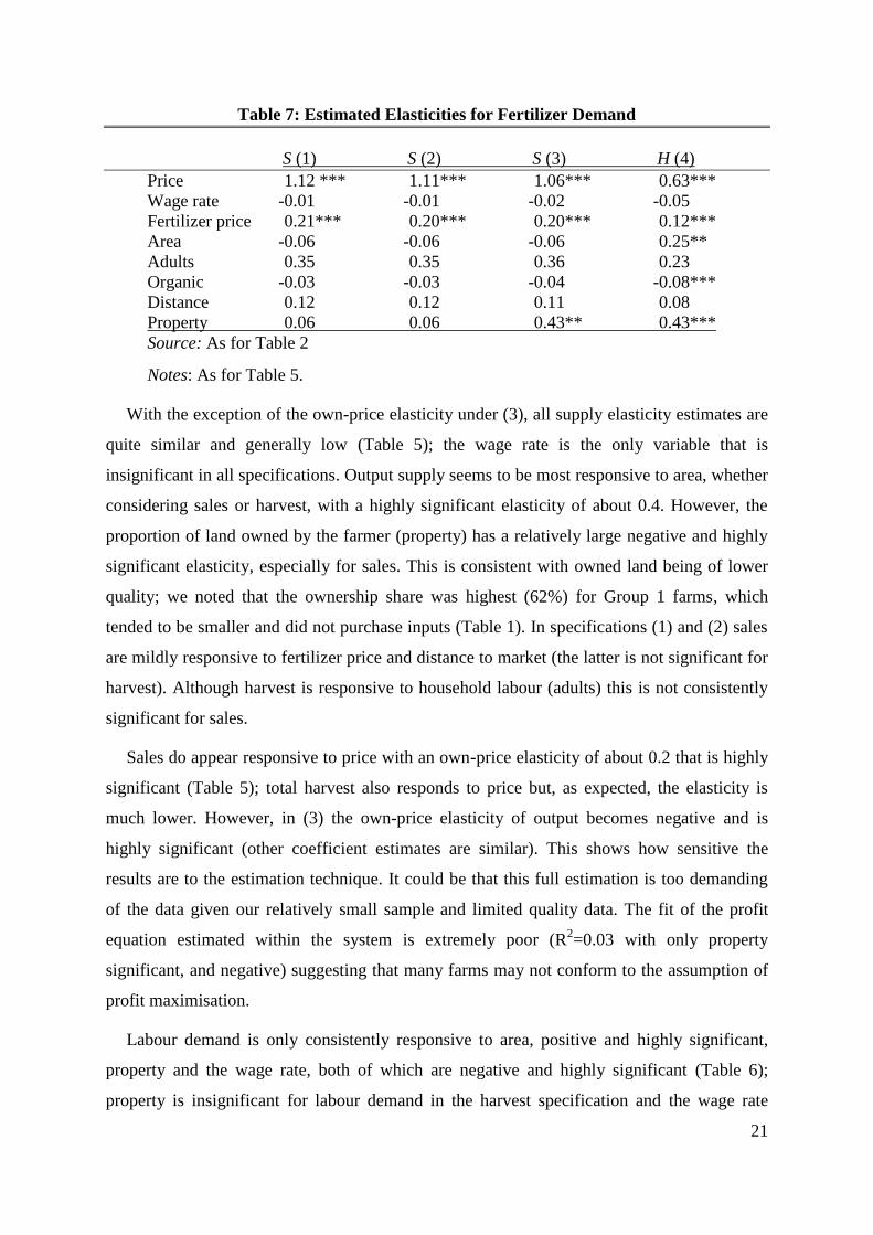
Table 7: Estimated Elasticities for Fertilizer Demand

S (1) S (2) S (3) H (4)

Price 1.12 *** 1.11*** 1.06*** 0.63***

Wage rate -0.01 -0.01 -0.02 -0.05

Fertilizer price 0.21*** 0.20*** 0.20*** 0.12***

Area -0.06 -0.06 -0.06 0.25**

Adults 0.35 0.35 0.36 0.23

Organic -0.03 -0.03 -0.04 -0.08***

Distance 0.12 0.12 0.11 0.08

Property 0.06 0.06 0.43** 0.43***

Source: As for Table 2

Notes: As for Table 5.

With the exception of the own-price elasticity under (3), all supply elasticity estimates are

quite similar and generally low (Table 5); the wage rate is the only variable that is

insignificant in all specifications. Output supply seems to be most responsive to area, whether

considering sales or harvest, with a highly significant elasticity of about 0.4. However, the

proportion of land owned by the farmer (property) has a relatively large negative and highly

significant elasticity, especially for sales. This is consistent with owned land being of lower

quality; we noted that the ownership share was highest (62%) for Group 1 farms, which

tended to be smaller and did not purchase inputs (Table 1). In specifications (1) and (2) sales

are mildly responsive to fertilizer price and distance to market (the latter is not significant for

harvest). Although harvest is responsive to household labour (adults) this is not consistently

significant for sales.

Sales do appear responsive to price with an own-price elasticity of about 0.2 that is highly

significant (Table 5); total harvest also responds to price but, as expected, the elasticity is

much lower. However, in (3) the own-price elasticity of output becomes negative and is

highly significant (other coefficient estimates are similar). This shows how sensitive the

results are to the estimation technique. It could be that this full estimation is too demanding

of the data given our relatively small sample and limited quality data. The fit of the profit

equation estimated within the system is extremely poor (R2=0.03 with only property

significant, and negative) suggesting that many farms may not conform to the assumption of

profit maximisation.

Labour demand is only consistently responsive to area, positive and highly significant,

property and the wage rate, both of which are negative and highly significant (Table 6);

property is insignificant for labour demand in the harvest specification and the wage rate

22

elasticity is lower. Specification (1) differs, with significant price elasticity and insignificant

wage rate, but this is probably because there is no control for farms that do not hire labour.

Specification (2) is the most relevant for labour demand and shows it increases with area but

decreases with ownership and the wage rate.

Fertilizer demand seems to be extremely responsive to output price, with an elasticity of

above unity in the sales specifications (Table 7). Fertilizer demand is also quite responsive to

fertilizer price, with an elasticity of about 0.2; surprisingly perhaps this is positive. This may

simply be a feature of the cross-section data, with farmers that are able to afford more

fertilizer buying a more expensive variety. Another possibility is inter-linked transactions

where farmers using fertilizer are subject to contractual arrangements which tie them to buy

fertilizer from traders at an above market price, whilst in exchange traders buy their output at

a favourable price. Benson et al (2012) mention the existence of such types of arrangements

in Tanzania.

Area is insignificant for fertilizer demand, which does not come as a surprise given the

very large proportion of non-users. The exception is in the harvest specification where area

has a positive significant elasticity and organic fertilizer is negative and insignificant. This

result is consistent with larger farms that do have access to sufficient organic fertilizer being

more likely to demand inorganic fertilizer. It may more simply reflect weaknesses in the data,

and we noted in table 4 that the Probit for (4) was the weakest of those estimated.

Perhaps the most unusual results is that the property variable is positive and quite

significant in (3) and (4). As we have seen that ownership appears to be associated with lower

output, why would it be associated with higher demand for fertilizer? It would be mistaken to

read too much into this as specifications (3) and (4) are the most weakly performing models.

However, the pattern of results for this ownership measure suggest that there are differences

between the land that farmers own and land they operate in some form of rental arrangement.

It may be that there are multiple differences we have not been able to account for, i.e. some

farmers own poor quality land with low levels of (marketed) output and purchased inputs, but

there are also some who own higher quality land and purchase fertilizer to increase marketed

output. In future research incorporating tree crops and the later NPS wave to increase the

sample size we may be able to investigate this further.

23

5 Conclusions and discussion

This study assessed the extent to which price responsiveness is observed in Tanzanian

agriculture using farm-level data for long season food crops from the first wave of the NPS of

2008/09. A significant degree of responsiveness is found and many results are consistent with

the existing literature. Marketed output is responsive to price, fertilizer demand is responsive

to prices (of output and fertilizer) and labour demand responds to the wage rate. However,

non-price factors, especially area cultivated and the weighted property index, are found to be

highly significant, confirming that supply response is not simply about prices. We have

identified an interesting effect with the ownership variable which may hide serious

constraints on land and calls for a deeper analysis of land structure and tenancy.

Fertilizer use is found to be highly responsive to output price but there is a positive

fertilizer price elasticity; fertilizer use may be a criterion for differentiation between the more

richer commercial farms and more traditional near subsistence farms. An important caveat is

that results are highly dependent upon the specification used and there are serious limitations

in the data.

Further research should disaggregate the data further (by crops and agro-climatic zones) to

get better insights into regional disparities and cropping pattern structures. Using the three

waves of the NPS is also desirable so as to include a temporal dimension to the analysis.

Although only using part of the data in the first wave, we have identified challenges and

constraints shaping the Tanzanian agricultural sector that need to be accounted for if this

sector is to achieve a successful development through productivity enhancement, income

generation, reducing unemployment (especially youth unemployment) and a decline in rural

poverty.

A major finding is that there is something about inorganic fertilizer in Tanzania, in the

sense that results show extreme output price responsiveness, and summary statistics clearly

show that the discrimination between large and smaller producers is made on the basis of

whether fertilizer is used or not. In this respect, fertilizer use appears much more

discriminatory than hiring labour. This may hide social characteristics only common to those

farmers buying fertilizer. Fertilizer adoption may be linked to social characteristics that have

not been captured in the analysis (one possible salient feature is the complex bureaucracy and

corruption involved in the supply and distribution chain of fertilizers). It appears that farmers

who buy fertilizer do so because they can afford it. According to Minot (2009), 63% of

24

farmers in Tanzania who did not buy fertilizer reported this was due to prices being too high;

the source of finance is farm income in 69% of cases, whereas credit is only a source of

finance in 2% of all cases, an indicator of barriers faced by poor farmers. Perception of risk is

also important, since more risk aversion among poorer farmers may greatly limit adoption.

More generally, there may be phenomena of virtuous circles taking place: successful use of

fertilizer in a given season will increase yields and generate cash, making it easier to buy

fertilizer in the next season. The extent to which such use is successful could be endogenous.

In terms of the groups identified, the households not buying any variable input may not

conform to the assumption of profit maximisation (confounding interpretation of the

econometric estimates). However, given our results, especially those regarding how

important fertilizer adoption is, it could be that farms hiring labour only do not meet this

assumption either (which is consistent with the marked differences observed between group 2

and group 3). For these households, a Leontief production function with fixed use of inputs

may be more appropriate than the standard profit-maximising flexible production function.

Several policy implications can be derived with considerable caution. Improving the

functioning of factor markets is obviously important and not controversial. This is well

established for credit markets and the implications for access to fertilizer but our results

suggest that there may also be major constraints associated with the operation of land

markets. Land ownership is not associated with the positive effects one might expect to see.

Our results would not justify advocating subsidies to promote increased fertilizer use but it

does seem important to promote knowledge of effective fertilizer use, perhaps through

targeted extension services.

Output does respond to prices but area cultivated is the major determinant of sales and

output. This does not imply advocating larger scale farming (a more thorough investigation of

yields and farm size is necessary for any such recommendations). Given farm size, access to

fertilizer and labour can increase output; this is quite well known and our analysis merely

confirms the constraints faced in utilising purchased inputs. The more surprising finding is

that there is no obvious benefit, in terms of increased sales or output, associated with owning

land, suggesting that further analysis of land markets is warranted.

25

References

Abrar, S., O. Morrissey and A. Rayner (2004a), Aggregate Agricultural Supply Response in

Ethiopia: A Farm-level Analysis’, J. of International Development, 16:4, 605-620

Abrar, S., O. Morrissey and A. Rayner (2004b), ‘Crop-level Supply Response by Agro-

climatic Regions in Ethiopia’ Journal of Agricultural Economics, 55:2, 289-312

Abrar, S., and O. Morrissey (2006), ‘Supply Response in Ethiopia: Accounting for Technical

Inefficiency’ Agricultural Economics, 35 (3), 303-317

Ahmed, S., Diffenbaugh, N., Hertel, T. and Martin, J. (2012), Agriculture and Trade

Opportunities for Tanzania: Past Volatility and Future Climate Change, Review of

Development Economics, 16 (3), 429-447

Anderson, K., W. Martin, D. Sandri and E. Valenzuela (2006), Methodology for Measuring

Distortions to Agricultural Incentives, Agricultural Distortions Research Project Working

Paper 02, World Bank, Washington DC, August.

Anderson, K. and W. Masters (eds, 2009), Distortions to Agricultural Incentives in Africa,

Washington DC: World Bank

Arndt, C., Farmer, W., Strzepek, K. and Thurlow, J. (2012), Climate Change, Agriculture and

Food Security in Tanzania, Review of Development Economics, 16 (3), 378-393

Benson, T., Kirama, S., & Selejio, O. (2012), The supply of inorganic fertilizers to smallholder

farmers in Tanzania, Washington DC: IFPRI discussion paper 01230.

Fan, S., Nyange, D. and Rao, N. (2012), Public Investment and Poverty Reduction in

Tanzania: Evidence from Household Survey Data, Chapter 6 in T. Mogues and S. Benin

(eds), Public Expenditures for Agriculture and Rural Development in Africa, London:

Routledge, pp 154-177

Hattink, W., Heerink, N., & Thijssen, G. (1998), Supply response of cocoa in Ghana: A farm-

level profit function analysis, Journal of African Economies, 7 (3), 424-444.

Ogbu, O. M., and Gbetibouo, M. (1990), Agricultural supply response in sub-Saharan Africa:

A critical review of the literature, African Development Review, 2 (2), 83-99.

Leyaro, V. and O. Morrissey (2013), ‘Expanding Agricultural Production in Tanzania: Scoping

Study for Tanzania IGC on National Panel Surveys’, IGC Tanzania

McKay, A., O. Morrissey and C. Vaillant (1999), ‘Aggregate Agricultural Supply Response in

Tanzania’, J. Int. Trade and Economic Development, 8:1, 107-123

Minot, N. (2009), Fertilizer policy and use in Tanzania, paper prepared for the Fertilizer Policy

Symposium of the COMESA African Agricultural Markets Programme (AAMP), Livingstone,

Zambia.

Morrissey, O. and V. Leyaro (2009), ‘Distortions to Agricultural Incentives in Tanzania’, in K.

Anderson and W. Masters (eds.), chapter 11, pp. 307-328

Skarstein, R. (2005), Economic Liberalisation and Smallholder Productivity in Tanzania: From

Promised Success to Real failure, 1985-1998, Journal of Agrarian Change, 5 (3), 334-

362.

World Bank (1994), Tanzania Agriculture: A Joint Study by the Government of Tanzania and

the World Bank, Washington DC: The World Bank

World Bank (2006), Tanzania: Sustaining and Sharing Economic Growth, Country Economic

Memorandum and Poverty Assessment, Volume 1 (draft, 28 April).

Designed by soapbox.co.uk

The International Growth Centre (IGC) aims to promote sustainable growth in developing countries by providing demand-led policy advice based on frontier research.

Find out more about our work on our website www.theigc.org

For media or communications enquiries, please contact mail@theigc.org

Subscribe to our newsletter and topic updates www.theigc.org/newsletter

Follow us on Twitter @the_igc

Contact us International Growth Centre, London School of Economic and Political Science, Houghton Street, London WC2A 2AE