Fog removal for Automobile Electronic Mirror

M.Sc in Computer Science

Internship report

Soheila Kiani

Supervisors:Professor Max Mignotte

Hyunjin Yoo

Faurecia IRYStec Inc.Montreal, Canada

July 5, 2021

Acknowledgement

I undertook this internship under the supervision of Professor Max Mignotte at University of

Montreal and guidance of Yyunjin Yoo, head of reseach team at IRYStec.

I would like to thank my supervisor Professor Max Mignotte who kindly supported me and

gave me several appropriate suggestions about my tasks during the internship.

I’m also grateful to the IRYStec staff for their patience and assistance during my training at

their company. It was a great learning experience for me to work with their research team who

are really expert and creative people with lots of innovative ideas.

i

Abstract

This report explains the internship project done as a Research Intern in the research team of

Faurecia IRYstec company. The project title is "fog removal for automobile electronic mirror"

which is known as "E-Mirror" at IRYStec.

After surveying about state of the art, Contrast Limited Adaptive Histogram Equalization

(CLAHE) is implemented and merged with current product of IRYStec "Perceptual Display

Platform Vision (PDP Vision)" for better results. Some other approaches are also implemented

and evaluated during this internship. Moreover, Image Quality Assessment (IQA) and com-

parison with competitor is done.

ii

Contents

Acknowledgement i

Abstract ii

1 Introduction 1

1.1 Faurecia IRYStec Inc. . . . . . . . . . . . . . . . . . . . . . . . . . . . . . . . . . . 1

1.2 Problem Statement . . . . . . . . . . . . . . . . . . . . . . . . . . . . . . . . . . . 2

2 Fog removal Approaches 4

2.1 Image Restoration (Model based techniques) . . . . . . . . . . . . . . . . . . . . 4

2.2 Image Enhancement Techniques (Non model based) . . . . . . . . . . . . . . . . 5

3 CLAHE 6

3.1 Algorithm . . . . . . . . . . . . . . . . . . . . . . . . . . . . . . . . . . . . . . . . 6

3.2 Implementation . . . . . . . . . . . . . . . . . . . . . . . . . . . . . . . . . . . . . 10

3.3 Tuning CLAHE parameters . . . . . . . . . . . . . . . . . . . . . . . . . . . . . . 12

3.4 Performance . . . . . . . . . . . . . . . . . . . . . . . . . . . . . . . . . . . . . . . 14

3.5 Merge with PDP . . . . . . . . . . . . . . . . . . . . . . . . . . . . . . . . . . . . . 15

3.5.1 Tone Curve Selection . . . . . . . . . . . . . . . . . . . . . . . . . . . . . . 16

3.6 Improvement Ideas . . . . . . . . . . . . . . . . . . . . . . . . . . . . . . . . . . . 17

3.6.1 Detect Foggy Images . . . . . . . . . . . . . . . . . . . . . . . . . . . . . . 17

3.6.2 Guided Filter . . . . . . . . . . . . . . . . . . . . . . . . . . . . . . . . . . 18

3.6.3 Homomorphic Filtering . . . . . . . . . . . . . . . . . . . . . . . . . . . . 18

3.6.4 Learning Approaches . . . . . . . . . . . . . . . . . . . . . . . . . . . . . 20

4 Image Quality Assessment 22

iii

5 Hardware Configuration 25

6 Conclusions 27

iv

1 | Introduction

This chapter contains two short subsections. The first subsection introduces IRYStec company

and its research team. Second subsection is the problem statements that we worked on it

during the internship.

This report also includes five other chapters. The second chapter briefly reviews some

literature about fog removal and dehazing. Chapter three is dedicated to the main tasks of

internship project. Some theoretical and practical studies were done about the contrast limited

adaptive histogram equalization. The performance is a key point in this project so different

implementations were done and evaluated. The fog removal approach was merged with one

of the current products of the company. Moreover, some issues were encountered during the

implementation and based on the results, some other modifications and improvements were

performed too.

Chapter four describes image quality assessment and how this project is evaluated. Hard-

ware configuration is explained in chapter five. The last chapter is conclusion of the report.

1.1 Faurecia IRYStec Inc.

IRYStec Inc. 1 was an startup company which is founded in 2015. IRYStec announced the ac-

quisition of the company by Faurecia as of April 2020, so the name of the company changed to

“Faurecia IRYStec Inc.” Faurecia is a French global automotive supplier. It is one of the largest

international automotive parts manufacturer in the world for vehicle interiors and emission

control technology.

Automotive OEMs and Tier 1s are collaborating with IRYStec to provide a software plat-

1https://www.irystec.com/

1

form that intelligently adapts the displayed content to the ambient light driving conditions,

panel technology and the driver’s unique vision to deliver a safer and more power efficient

in-car viewing experience for drivers and passengers .

Perceptual Display Platform Vision (PDP Vision) technology is the main product of the

company which is a customizable and scalable software solution that integrates seamlessly

into the primary automotive display systems.

IRYStec company consists of a general manager, an HR expert, research, engineering and

sales teams. Every team has a head member and the members of each team are under the

supervision of the head. My internship was done in the research team. This team has a head,

3 researchers and 3 research interns. The main task of research team is to investigate new

approaches which is related to perceptual vision such as aging, perceptual 3D, attention re-

targeting and so on. The projects are predefined in the road map of the company. The other

task is to evaluate engineering team’s work. Researchers implement their ideas and findings

using Python or Matlab. The codes should be readable and executable by some standards of

the company. These codes are used later as a reference for engineering team to implement

a new product or modify current products. It is also a reference to evaluate final product’s

output and comparison with competitor’s result.

The research team has weekly meetings to present their progress, share their results, dis-

cuss their problems with each others and receive feedback from others. Every team member

has a one to one weekly meeting with the head to explain their projects in more detail. There

is also a one hour happy discussion weekly to talk about new ideas in image processing and

computer vision field which are not on the road map. Every one can be volunteer to present

papers, codes and other interesting findings with other.

1.2 Problem Statement

Fog, haze and smoke are a big reason of road accident because of reducing visibility range.

Table 1.1: Visibility range based on weather condition

Meteorological condition Visibility ranges (meters)Fog Cloudy Up to 1000Mist Moist 1000-2000Haze Dry 2000-5000

2

Foggy and hazy weather conditions often create difficulty in capturing clear images. Ef-

fect of fog mainly is caused by two phenomenon. First, fog disperses the imitated light of

scene. Second, it scatters atmospheric light toward the camera (1). As a result, it extremely

reduces the visibility of the image and cause higher noise, more blurring, lower contrast as

well as color decay. Meanwhile, the foggy image always contributes the negative effect in the

perception applications such as environment monitoring and autonomous robot navigation.

It is particularly important to eliminate the adverse factor to enhance the image quality for

visualization.

One of the innovations in brand new automobiles is to use digital cameras instead of side

mirrors. These two cameras capture scenes of environment and the result will be shown on

monitors inside the car. Therefore, it is possible to enhance captured scene to improve percep-

tual quality and increase drivers’ visibility. The current product of the company adjust image

color and brightness in different weather and light conditions. The next step is the topic of this

internship. The purpose is to improve foggy images to increase visibility which cause more

safety for drivers.

3

2 | Fog removal Approaches

The first step in this internship was to do a survey about fog removal approaches to under-

stand the context and possibilities better. In this chapter, the result of this survey is discussed

shortly.

There are various classifications for fog removal approaches from different perspectives.

The way which is used here matches more to current requirements of the company. In this

view, there are two main classes of image restoration and image enhancement approaches. In

some papers refer to image restoration and image enhancement methods as model based and

none model based based techniques respectively.

Moreover, some new approaches combine two or more different approaches such as CLAHE

with guided filter for better result (2).

Furthermore, some learning approaches utilize machine learning techniques, specially deep

learning techniques for fog removal. They can be applied on both restoration and enhancement(3).

The learning approaches are not in the scope of this internship, however, as an open source

promising approach was referred by another research team member in the company, it is eval-

uated which will be discussed later in the next chapter.

The two main approaches are described in the following sections.

2.1 Image Restoration (Model based techniques)

The main purpose of image restoration is to undo defects which degrade an image. To achieve

this goal, it requires extra information about image environment. In this way, physical models

are used to forecast the pattern of image degradation information. Restoration techniques can

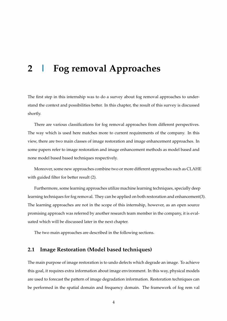
be performed in the spatial domain and frequency domain. The framework of fog rem val

4

using image restoration techniques is shown in figure 2.1.

Figure 2.1: framework for fog removal

Fog can be considered as blur; therefore, defogging improves the quality of image using

blur estimation. The methods in this category can be divided to single or multiple foggy image

approaches. To extract information about the fog in multiple foggy images, multiple images

captured under the same meteorological weather conditions of the sight or multiple images

captured under different meteorological weather condition of the sight. However, for single

foggy images there is only one image. One of the most well known approaches for single

image restoration is dark channel prior single image-based restoration(4).

As we need a real time approach, we do not have the possibility to use multiple images

approaches.

2.2 Image Enhancement Techniques (Non model based)

The main purpose of image enhancement technology is to enhance the useful potential infor-

mation and eliminate the unnecessary noise simultaneously. Unlike restoration techniques,

in this approach, there is no need to collect extra information about input images. Histogram

equalization is the most common method of non model based enhancement. Histogram equal-

ization is a contrast enhancement technique that adjusts pixels intensities in order to obtain

new enhanced image with usually increased global contrast (5). These techniques can be done

in spacial and frequency domain. CLAHE and Wavelet Transform are sample techniques in

spatial and frequency domain respectively.

5

3 | CLAHE

In this project, IRYStec Inc. searched for a practical approach with high level performance.

Contrast Limited Adaptive Histogram Equalization (CLAHE) is a candidate as it was known

that some of the competitors used this approach in their product. Therefore the feasibility of

this approach as a final product is guaranteed. It was studied in detail and implemented from

scratch to gain a deep understanding.

CLAHE is a variant of Adaptive Histogram Equalization (AHE). AHE differs from orig-

inal Histogram Equalization (HE) in the respect that the adaptive method calculates several

histograms, each corresponding to a distinct non-overlapping section of the image called tile

or grid, and uses them to redistribute the lightness values of the image. It improves the lo-

cal contrast and enhances the edges in each tile. After enhancement, in reconstruction phase

neighboring tiles are then combined using an interpolation function to remove the artificial

boundaries.

The major drawback of AHE is its tendency to amplify noise in relatively homogeneous

regions. CLAHE prevents it by limiting the amplification.

CLAHE can be applied on color images, for this purpose, the luminance component is

extracted from RGB image and after enhancing luminance component, the color image will be

reconstructed again.

3.1 Algorithm

The algorithm is described as following step (2, 6, 7, 8):

1. Dividing the original intensity image into non-overlapping contextual regions. The total

number of image tiles is equal to M × N, and 8 × 8 is good value to preserve the image

6

chromatic data.

2. Calculating the histogram of each contextual region according to gray levels present in

the array image.

3. Calculating the contrast limited histogram of the contextual region by CL values as:

Navg = (NrX ∗ NrY)/Ngray

where Navg is the average number of pixel, Ngray is the number of gray levels in the

contextual region, NrX and NrY are the numbers of pixels in the X dimension and Y

dimension of the contextual region.

The actual CL can be expressed as:

NCL = Nclip ∗ Navg

where NCL is the actual CL, Nclip is the normalized CL in the range of [0,1]. if the number

of pixels greater than NCL, the pixels will be clipped, The total number of clipped pixels

is defined as N∑ clip, then the average of the remain pixels to distribute to each gray level

is:

Navggray = N∑ clip/Ngray

The histogram clipping rule is given by the following statements:

I f Hregion(i) > NCLthen

Hregion_clip(i) = NCL

Elsei f (Hregion(i) + Navggray) > NCLthen

Hregion_clip(i) = NCL

ElseHregion_clip(i) = Hregion(i) + NCL

where Hregion(i) and Hregion_clip(i) are original histogram and clipped histogram of each

region at i-th gray level.

7

4. Redistribute the remain pixels until the remaining pixels have been all distributed. The

step of redistribution pixels is given by

Step = Ngray/Nremain

where Nremain is the remaining number of clipped pixels. Step is positive integer at least

1. The program starts search from the minimum to the maximum of gray level with the

above step. If the number of pixels in the gray level is less than NCL, the program will

distribute one pixel to the gray level. If the pixels are not all distributed when the search

is end, the program will calculate the new steps according to Step formula and start new

search round until the remaining pixels is all distributed.

Figure 3.1: Original Histogram

Figure 3.2: Clipped Histogram

5. The gray level histogram which is limited contrast in each contextual region is processed

by histogram equalization.

6. The points in the center of the contextual region are regarded as the sample points.

7. Calculating the new gray level assignment of pixels within a sub-matrix contextual re-

gion by using a bi-linear interpolation between four different mappings in order to elimi-

nate boundary artifacts. The transformation functions are appropriate for the tile sample

points, black squares in the left part of the figure. There are different types of transfor-

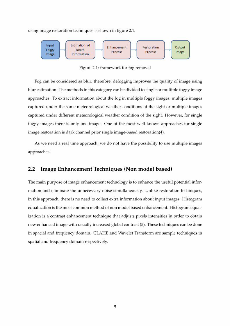
mations that can be used. Figure x shows different transformations:

8

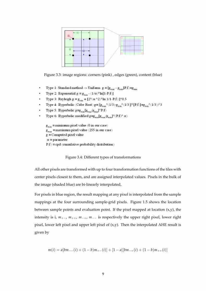
Figure 3.3: image regions: corners (pink) , edges (green), content (blue)

Figure 3.4: Different types of transformations

All other pixels are transformed with up to four transformation functions of the tiles with

center pixels closest to them, and are assigned interpolated values. Pixels in the bulk of

the image (shaded blue) are bi-linearly interpolated,

For pixels in blue region, the result mapping at any pixel is interpolated from the sample

mappings at the four surrounding sample-grid pixels. Figure 1.5 shows the location

between sample points and evaluation point. If the pixel mapped at location (x,y), the

intensity is i, m+−, m++, m−+, m−− is respectively the upper right pixel, lower right

pixel, lower left pixel and upper left pixel of (x,y). Then the interpolated AHE result is

given by

m(i) = a[bm−−(i) + (1 − b)m+−(i)] + [1 − a][bm−+(i) + (1 − b)m++(i)]

9

Figure 3.5: Sample and evaluation points

where:

a =y − y−

y+ − y−, b =

x − x−x+ − x−

The interpolation coefficients reflect the location of pixels between the closest tile center

pixels, so that the result is continuous as the pixel approaches a tile center.

Pixels in the borders of the image outside of the sample pixels need to be processed spe-

cially. pixels close to the boundary (shaded green) are linearly interpolated, and pixels

near corners (shaded red) are transformed with the transformation function of the cor-

ner tile. This procedure reduces the number of transformation functions to be computed

dramatically and only imposes the small additional cost of linear interpolation.

3.2 Implementation

Some open source codes were found for CLAHE. By getting help from different sources first

implementation was done in Python. The implementation has the following functions as it is

shown in figure 3.6.

1. GetLuminance: The input image is a RGB color image, so before applying CLAHE, we

need the luminance component. There are some functions in image processing libraries

such as openCV or skimage for this purpose. It is possible to change RGB image to

grayscale one. The other option is to map RGB to LAB space. CLAHE is applied on

luminance component (L). At the end LAB image with new luminance (L) is converted to

RGB image. It was the first approach which was implemented. However, this approach

caused some changes in the color of original image. Therefore another way to extract

10

Figure 3.6: CLAHE implementation

luminance of sRGB values was utilized based on (9). This approach is the same as current

product of IRYStec. The other functions (next steps) apply on luminance component of

the image and at the end the contrast of original foggy images is adjusted based on

contrast ratio which is calculated based on the original luminance and the enhanced one

(10).

2. CreateHistogram: The luminance component has only one channel and same height and

width as color image can be considered as a two dimensional matrix. This matrix is

divided to non-overlapping tiles based on the tile size as the input parameter. It should

be mentioned that if image dimension is not dividable by tile size, image should be

extended by zero padding before this step. And before final step, the extended zero

pixels should be removed.

3. ClipHistogram: This method was implemented as explained in the original reference.

However, this part had some performance issue. In some other implementations such

as OpenCV, the remaining pixels are adjusted differently or ignored completely. The

ignorance causes that some pixels have values greater values than clip limit.

4. MapHistogram: The following image describes the mapping process very clearly. Ac-

cording to the pixel values, the probability of each intensity value, then the cumulative

probability and finally new intensity values are calculated. The mapping should be done

for each tile separately. In figure 3.7 the original values are between 1 and 10 and the new

range is 1 and 20. The values for 9 and 10 are 0, which means that in current tile, there is

no pixel with 9 or 10 values. In real case the range was fixed to [0,256). However, in some

resources, the number of bins considered as an input parameter and can be changed to

11

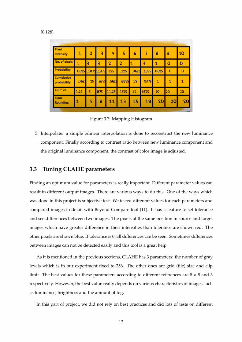
[0,128).

Figure 3.7: Mapping Histogram

5. Interpolate: a simple bilinear interpolation is done to reconstruct the new luminance

component. Finally according to contrast ratio between new luminance component and

the original luminance component, the contrast of color image is adjusted.

3.3 Tuning CLAHE parameters

Finding an optimum value for parameters is really important. Different parameter values can

result in different output images. There are various ways to do this. One of the ways which

was done in this project is subjective test. We tested different values for each parameters and

compared images in detail with Beyond Compare tool (11). It has a feature to set tolerance

and see differences between two images. The pixels at the same position in source and target

images which have greater difference in their intensities than tolerance are shown red. The

other pixels are shown blue. If tolerance is 0, all differences can be seen. Sometimes differences

between images can not be detected easily and this tool is a great help.

As it is mentioned in the previous sections, CLAHE has 3 parameters: the number of gray

levels which is in our experiment fixed to 256. The other ones are grid (tile) size and clip

limit. The best values for these parameters according to different references are 8 × 8 and 3

respectively. However, the best value really depends on various characteristics of images such

as luminance, brightness and the amount of fog.

In this part of project, we did not rely on best practices and did lots of tests on different

12

foggy and not foggy images. For grid size 4 × 4, 8 × 8, 16 × 16 and 32 × 32 are tested. A range

of values between 2 and 12 are also considered for clip limit test.

IRYStec has a great image and video dataset for testing different aspects of images, it con-

tains more than 100 images.

Figure 3.8 is an example of applying CLAHE on a foggy image. The grid size is 32 × 32 in

this sample. In first row, left image is the original one and right image is processed by CLAHE

with clip limit 4. The second row from left to right shows processed images by CLAHE with

clip limit 8 and 12 respectively. In the original scene the pedestrian can not be seen easily but

in the enhanced images it is more visible.

Figure 3.8: Original image and its enhancements by CLAHE, grid size: 32 × 32, clip limits:4,8,12

The test result for different parameter values on various images can be summarized as

follow:

1. for the clip limit:

(a) + Larger clip limit: more contrast enhancement

(b) - Very large clip limits: not a natural scene and boosted noise

(c) 3 the best values in most cases

13

2. for the grid size

(a) + Larger grid size: brighter images

(b) + Larger grid size: more local contrast enhancement and more details

(c) + Larger grid size: less computation time

(d) - Larger grid size: adds boarder effects and not as good as small ones

(e) 8 × 8 is the best value in most cases

Moreover according to references, some objective measurements such as Absolute Mean

Brightness Error (AMBE), Absolute Deviation in Entropy (ADE), Peak Signal to Noise Ratio

(PSNR), Variance Ratio (VR), Structural Similarity Index Matrix (SSIM) Saturation Evaluation

Index (SEI) can be used for this purpose (12). It will be more discussed in evaluation section.

According to another reference (13) image entropy is also used to determine optimum

value for the parameters. Entropy is a statistical measure of randomness that can be used

to characterize the texture of the input image. Entropy is defined as -sum(p.*log2(p)), where

p contains the normalized histogram counts. Image entropy becomes relatively low when

histogram is distributed on narrow intensity region. and it becomes high when histogram

is uniformly distributed. Therefore, the entropy of the histogram equalized image becomes

higher than that of the original input image. Therefore the optimum value for clip limit is the

one that maximizes the image entropy.

3.4 Performance

Being real time is the key point in this project. After the first implementation and evaluation

on different images, the value of grid size and clip limit is fixed to 8× 8 and 3 for performance

test.

At first the execution time of each functions which is discussed in section 3.2 was measured

on different images. The size of the input image and its content (pixel values) causes various

execution time. The requirement was to be able to process at least 60 frames per second to be

real time.

At this part of project, I tested CLAHE from OpenCV library. OpenCV is open source

14

and it has C++ and Python implementations. At first Python version of OpenCV CLAHE

was checked. Comparing to the implementation from scratch, it creates better result. After

discussing with Engineering team to be sure that they can use OpenCV or not, we decided to

continue with OpenCV CLAHE.

To have more realistic results, the implementation was done again in C++. Installation

and adding OpenCV libraries had some difficulties. The execution time measurement was

repeated. As there was a gap between what was required and what was measured, searching

for better way was continued.

Finally the OpenCV CLAHE is implemented by C++ GPU version. This is much more

faster and the performance was acceptable. There is not a complete documentation about

installation and setup of OpenCV especially for GPU version. Therefore this step took a bit

more time but the result was satisfying. Applying CLAHE with C++ GUP version takes 0 to 5

millisecond on each frame and the average time for 100 frames was 2.3 millisecond.

3.5 Merge with PDP

IRYStec PDP Vision software a set of algorithms that adapt to ambient lighting conditions,

significantly improving display visibility in extremely bright and dark environments. It also

compensates for the loss of contrast sensitivity and yellowing of the cornea by aging of the

user’s eye. It increases the safety and comfort of drivers and passengers, thus reducing the

risk of road accidents by adjusting lighting conditions as the Human Visual System (HVS).

As PDP Vision software has different modules and functions, there were some different

ways to merge CLAHE algorithm within it. Different possible combinations were done and

the results of them were compared to find the best place to put CLAHE algorithm into PDP

software. The color correction function of PDP did some improvements on processed images

by CLAHE. There are also two different modes of contrast enhancements in PDP: Global (on

whole image), Local (on image segments). The current product uses both of them. However,

as performance is an issue, the combination of CLAHE with only global enhancement was

tested and evaluated.

Figure 3.9 shows the result of merging CLAHE with PDP. In the first row, the left images is

"the original image" and the right one is processed by "PDP". The second row from left to right

15

shows processed images by "CLAHE with global PDP" and "CLAHE with PDP" respectively.

Figure 3.9: merging CLAHE and PDP result

3.5.1 Tone Curve Selection

In the original PDP, the tone curve selection (14) relies on some input parameters. However,

when CLAHE was combined with PDP, it was required to find a way to select suitable tone

curve based on original image characteristics because some input values affects the result of

applying CLAHE. After some tests and measurements, it was found that the optimum tone

curve can be selected based on the average luminance of input image instead of PDP input

parameters.

Based on 100 sample images the following results were gathered. (L) is the average lumi-

nance.

1. Day images: average luminance > 0.2

2. Night images: average luminance < 0.2

3. L > 0.5 -> best TC = 13.68

4. L < 0.5 and L > 0.2 -> best TC = 10.8

16

5. L < 0.2 and L > 0.1 -> best TC = 7.1

6. L < 0.1 -> best TC = 4.3

Based on these calculations, a linear formula was implemented to select tone curve based

on average luminance.

3.6 Improvement Ideas

During the team’s weekly meeting some issues were discussed which caused to do more re-

search about some different topics. Most cases were implemented by Python image processing

libraries or some open source code found and utilized to do evaluation and get some results.

The issues are categorized in the following subsections.

3.6.1 Detect Foggy Images

One of the early request was finding a way to detect if an image is foggy or not. Distinguish

foggy image from the others makes it possible to do not apply CLAHE when it is not required.

Moreover, there were some worries about missing the quality or changing the color or bright-

ness of the images as well. One of the possible techniques which was found is using Variation

of the Laplacian. The Laplacian operator is used to measure the second derivative of an im-

age. It highlights regions of an image containing rapid intensity changes.This approach is

often used for edge detection. If an image contains high variance then there is a wide spread

of responses, both edge-like and non-edge like, representative of a normal, in-focus image.

If the variance is low, then there is a tiny spread of responses, indicating there are very little

edges in the image. The more an image is blurred, the less edges there are. The trick here is

setting the correct threshold is domain dependent. If the threshold sets to a very low value,

it incorrectly marks images as blurry when they are not. On the other side, if the threshold is

too high,then images that are actually blurry will not be marked as blurry. It is obvious that in

this case we considered fog as a blur which is common in image processing approaches.

According to the measurements, we found at least we need to classify day and night scenes

before defining a threshold. Although we knew that the scenes will be road frames because of

using as a side mirrors in car, but they may vary from place to place and one fixed threshold

may not work correctly.

17

This issue was stopped and not continued as we found we have high performance. More-

over, after merging CLAHE and PDP, some not foggy images were also tested and the result

was acceptable. Therefore, there was no more need to separate images into 2 different cate-

gories.

3.6.2 Guided Filter

There is paper in 2020 which utilized CLAHE with guided filter (2). In test and evaluation

phase we taught that we may need more clip limit to reveal more details. But when the clip

limit increases, we also have more noise in the image specially the homogeneous regions.

Guided filter is a kind of edge-preserving smoothing filter.It can filter out noise or texture

while retaining sharp edges. Moreover the computational complexity is linear. Therefore if we

apply guided filter on CLAHE processed image, we expect to have details and less noise.

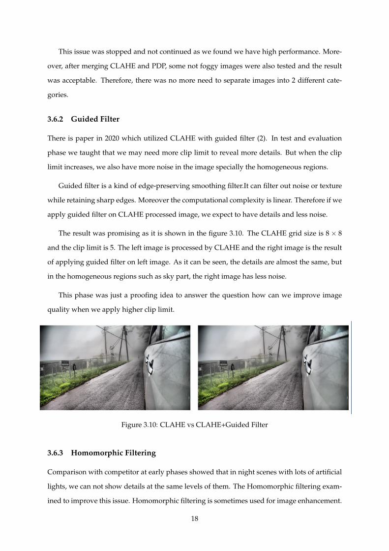
The result was promising as it is shown in the figure 3.10. The CLAHE grid size is 8 × 8

and the clip limit is 5. The left image is processed by CLAHE and the right image is the result

of applying guided filter on left image. As it can be seen, the details are almost the same, but

in the homogeneous regions such as sky part, the right image has less noise.

This phase was just a proofing idea to answer the question how can we improve image

quality when we apply higher clip limit.

Figure 3.10: CLAHE vs CLAHE+Guided Filter

3.6.3 Homomorphic Filtering

Comparison with competitor at early phases showed that in night scenes with lots of artificial

lights, we can not show details at the same levels of them. The Homomorphic filtering exam-

ined to improve this issue. Homomorphic filtering is sometimes used for image enhancement.

18

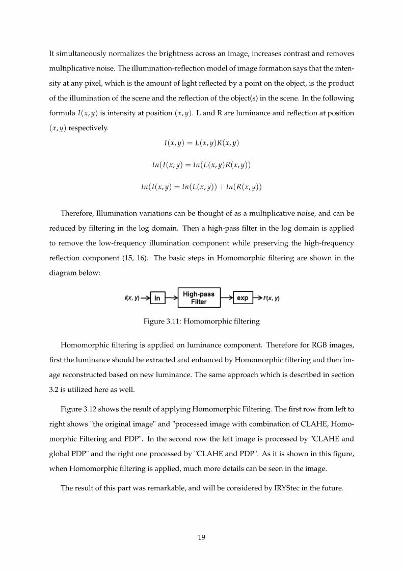
It simultaneously normalizes the brightness across an image, increases contrast and removes

multiplicative noise. The illumination-reflection model of image formation says that the inten-

sity at any pixel, which is the amount of light reflected by a point on the object, is the product

of the illumination of the scene and the reflection of the object(s) in the scene. In the following

formula I(x, y) is intensity at position (x, y). L and R are luminance and reflection at position

(x, y) respectively.

I(x, y) = L(x, y)R(x, y)

ln(I(x, y) = ln(L(x, y)R(x, y))

ln(I(x, y) = ln(L(x, y)) + ln(R(x, y))

Therefore, Illumination variations can be thought of as a multiplicative noise, and can be

reduced by filtering in the log domain. Then a high-pass filter in the log domain is applied

to remove the low-frequency illumination component while preserving the high-frequency

reflection component (15, 16). The basic steps in Homomorphic filtering are shown in the

diagram below:

Figure 3.11: Homomorphic filtering

Homomorphic filtering is app;lied on luminance component. Therefore for RGB images,

first the luminance should be extracted and enhanced by Homomorphic filtering and then im-

age reconstructed based on new luminance. The same approach which is described in section

3.2 is utilized here as well.

Figure 3.12 shows the result of applying Homomorphic Filtering. The first row from left to

right shows "the original image" and "processed image with combination of CLAHE, Homo-

morphic Filtering and PDP". In the second row the left image is processed by "CLAHE and

global PDP" and the right one processed by "CLAHE and PDP". As it is shown in this figure,

when Homomorphic filtering is applied, much more details can be seen in the image.

The result of this part was remarkable, and will be considered by IRYStec in the future.

19

Figure 3.12: Homomorphic filtering result

3.6.4 Learning Approaches

IRYStec currently do not work on machine learning approaches but as one of other interns

suggested a considerable work from his colleagues (3), we decided to investigate more.

Gated Context Aggregation Network a convolutional neural network for dehazing and

deraining. The trained model is open source and available online (17) and the only thing was

required to do is just to test with our sample images.

The presented sample results in the paper are really noticeable. However, when it was

applied on our sample images, the result was not proper and in some cases the output was

defective. Figure 3.13 and 3.14 show the input and output images from left to right respec-

tively. Figure 3.13 is one of the sample images which was referenced in the paper. The haze

was synthetic and it is not real. Figure 3.14 shows one real example of IRYStec samples. As it

can be seen the output image is not comparable with the output of Figure 3.13.

The reason that can explain this difference is that the network is trained with synthetic

foggy images not the real one. Sample hazy images are modified uniformly compared to

original images. However, in real foggy images the fog effect is not uniform in all parts of the

image. Furthermore, our real samples were different from training data set. Therefore it is

normal that it can not produce good results.

20

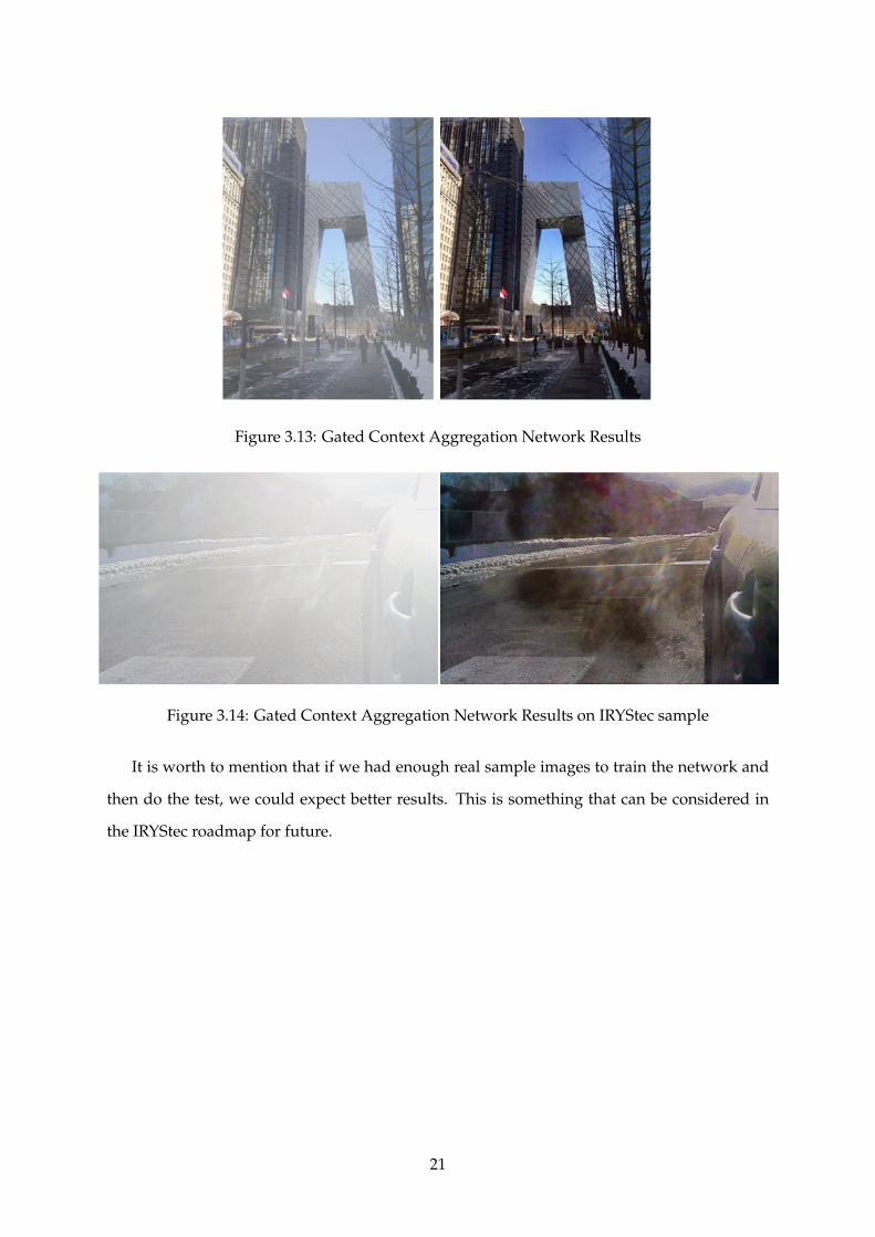
Figure 3.13: Gated Context Aggregation Network Results

Figure 3.14: Gated Context Aggregation Network Results on IRYStec sample

It is worth to mention that if we had enough real sample images to train the network and

then do the test, we could expect better results. This is something that can be considered in

the IRYStec roadmap for future.

21

4 | Image Quality Assessment

During different stages of this project, subjective test by research team was done. However,

after we found that results are good enough by human eyes, we started thinking to do some

measurements. It was a "necessity" when we wanted to compare with competitors and and

also for product presentation.

After having good results on images, processed video results was also created.

At first, as it is mentioned earlier we calculated ISSM and PSNR for original and processed

images as a evaluation metric. However, the value of these metrics were not compatible by

subjective test, so we decided to do some other Image Quality Assessment (IQA).

IQA algorithms take an arbitrary image as input and output a quality score as output.

There are three different types are IQA:

1. Full-Reference IQA: There is a ‘clean’ reference (non-distorted) image to measure the

quality of a distorted image (ex. Compressed image).

2. Reduced-Reference IQA: There is not a reference image, but an image having some selec-

tive information about it (e.g. watermarked image) to compare and measure the quality

of distorted image.

3. Objective Blind or No-Reference IQA: The only input is the image whose quality you

want to measure (distorted or modified image without any knowledge of distortion).

In this project we didn’t have any reference images so we decided to test some no-reference

IQA metrics.

For final evaluation original image with following processed images are considered:

1. CLAHE_LAB : image processed by CLAHE when luminance component is extracted by

22

converting RGB image to LAB image.

2. CLAHE_ColorCorrection: image processed by CLAHE when the luminance component

extracted from sRGB (9) and color correction function of PDP is applied.

3. CLAHE_GlobalPDP : image processed by CLAHE and PDP with only global contrast

enhancement.

4. CLAHE_PDP: image processed by CLAHE and PDP.

There are different no-reference metrics such as BRISQUE (18), PIQE and NIQE. Mentioned

processed images are created and these metrics are calculated for them.

Between these metrics BRISQUE performed better and showed more steady results and it

was compatible by subjective testing.

BRISQUE has a reference data set of images. different distortions such as noises, blurring

and compression are done with various degrees. There are 17 types of distortion and each

distortion is done in 4 different degree. Then some natural scene statistics extracted from

images. a support vector regressor trained on the data set. The input image receives a number

which define the quality of the image. BRISQUE score is in the range [0, 100] and lower values

of score reflect better perceptual quality of image (19).

Based on the BRISQUE metric on average, CLAHE_PDP is the best. The results are CLAHE_GlobalPDP

and CLAHE_ColorCorrection are almost the same and in the second rank.

Table 4.1: Average BRISQUE value on a data set of 100 images

BRISQUEOriginal image 36.8139CLAHE_LAB 26.2618CLAHE_ColorCorrection 26.1285CLAHE_GlobalPDP 25.5973CLAHE_PDP 20.2439

We also extracted some frames from one of the IRYStec competitor’s before-after result.

Run all processes on before images and compare with after result of competitor. On extracted

samples IRYStec CLAHE_PDP outperforms the competitor. An example of final results is

shown in figure 4.1. The left one is original images and the right one is the processed one by

IRYStec product.

23

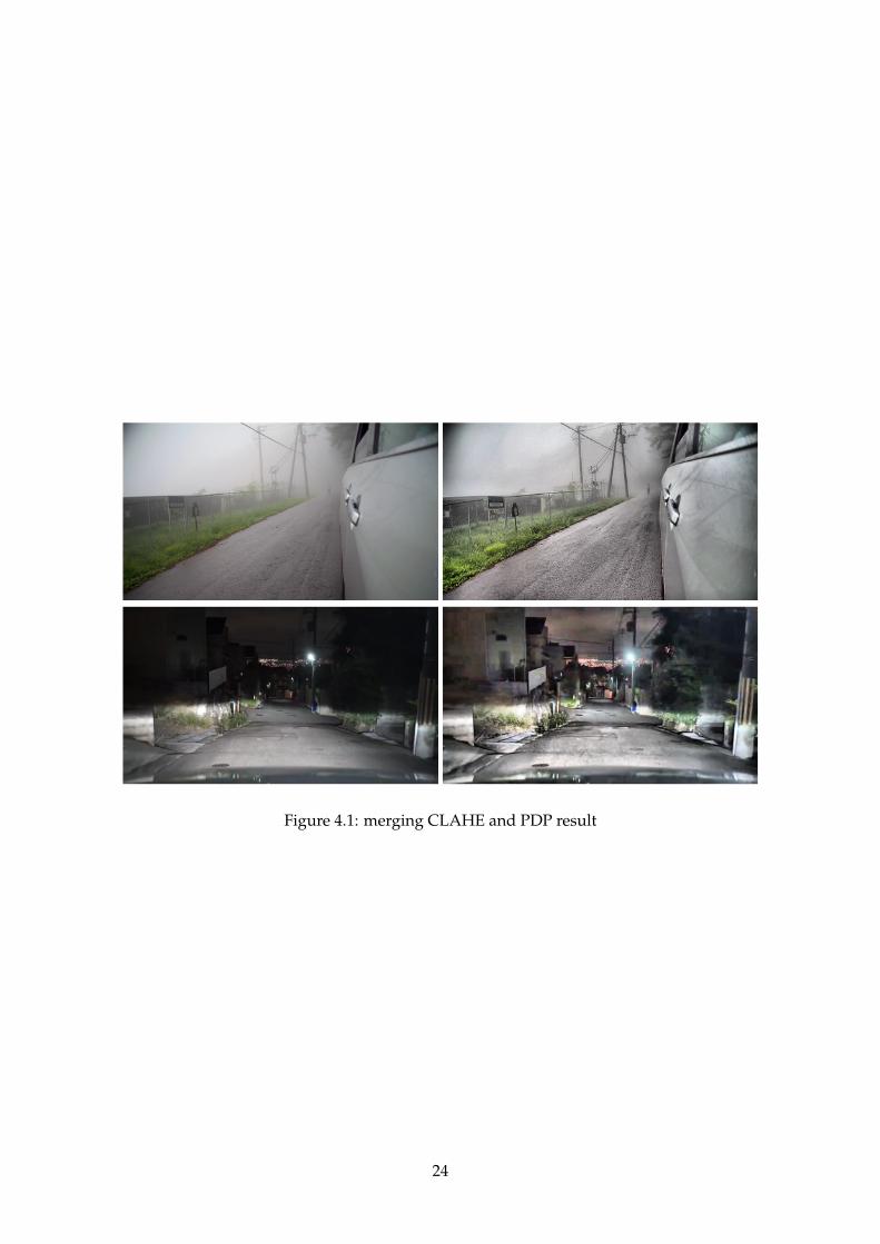
Figure 4.1: merging CLAHE and PDP result

24

5 | Hardware Configuration

All tests and evaluations performed in this internship were done on captured images and

videos. However, to evaluate the final product, it was required to simulate real environment.

For this purpose IRYStec bought a RVP-TDA4Vx multi-camera platform (20) and tow 2.1 MP

FPD-Link III camera module with SONY® IMX390 image sensor (21).

I had the chance to do the configuration of the platform and cameras on my last days. The

platform works with both Windows and Linux operating systems. Installing a serial terminal

such as PuTTy (22) makes it possible to run the commands. The platform has a SD card mem-

ory and it has also the option to add USB files. It is possible to save the raw frames and also

videos on external memory to do the process.

The output of this work for IRYStec is a complete documentation about configuration and

the issues encountered during setup and how to deal with. Moreover, some useful commands

sample to get frames and videos and save them on external USB file instead of internal SD

card was included. Figure 5.1 shows an image of configured camera with output on LCD on

my last internship day.

I also did some researches about how to create foggy images more than using software

libraries that do synthetic fog (23) and I recommended to buy some fog machine to create

more realistic inputs. This machines are portable and can be helpful to have better inputs to

test more precisely.

25

Figure 5.1: TDA4 platforms with cameras

26

6 | Conclusions

This internship was taken in IRYStec company research team on fog removal for automobile

electronic mirror project. During this project, I studied about different algorithms and possible

solutions for the problem. CLAHE was implemented with different programming languages

and platforms. Lots of test for quality assessment and performance check were done. The

detected issues on the results were investigated more and possible solutions for them are rec-

ommended. The hardware was configured for real test.

In a nutshell, this internship was an excellent and instructive experience for me. I can con-

clude that there was a lot learnt from my work at IRYStec as I had no prior practical experience

with image processing. I gained a desirable knowledge and skills in this field. In personal per-

spective view, attention to details, study more and be a questioner are the most significant

achievements during this project. It is needless to say that it is just a beginning for me and I

should continue learning.

27

Bibliography

[1] G Yadav, S Maheshwari, and A Agarwal. Fog removal techniques from images: A com-

parative review and future directions. In International Conference on Signal Propagation and

Computer Technology (ICSPCT), pages 44–52, 2014.

[2] S Badal and P Mathur. An improved image dehazing technique using clahe and guided

filter. In 7th International Conference on Signal Processing and Integrated Networks (SPIN),

2020.

[3] D Chen, M He, Q Fan, and Liao J. Gated context aggregation network for image dehazing

and deraining. In IEEE Winter Conference on Applications of Computer Vision (WACV), 2019.

[4] He Kaiming, Sun Jian, and Tang Xiaoou. Single image haze removal using dark channel

prior. IEEE Transactions on Pattern Analysis and Machine Intelligence, 33(12):2341 – 2353,

2011.

[5] https://en.wikipedia.org/wiki/Histogram_equalization.

[6] https://web.archive.org/web/20120113220509/http://radonc.ucsf.edu/research_

group/jpouliot/tutorial/HU/Lesson7.htm.

[7] Xu Zhiyuan, Liu Xiaoming, and Ji Na. Fog removal from color images using contrast

limited adaptive histogram equalization. In 2nd International Congress on Image and Signal

Processing, 2009.

[8] https://en.wikipedia.org/wiki/Adaptive_histogram_equalization.

[9] https://www.w3.org/TR/WCAG20/#relativeluminancedef.

[10] https://www.w3.org/TR/WCAG20/#contrast-ratiodef.

28

[11] https://en.wikipedia.org/wiki/Beyond_Compare.

[12] J Justin, J Sivaramanb, R Periyasamya, and V.R Simic. An objective method to identify

optimum clip-limit and histogram specification of contrast limited adaptive histogram

equalization for mr images. Biocybernetics and Biomedical Engineering, 37(3):489–497, 2017.

[13] B Min, D.K Lim, S.J Kim, and Lee J.H. A novel method of determining parameters of clahe

based on image entropy. International Journal of Software Engineering and its Applications, 7

(5):113–120, 2013.

[14] Eilertsen Gabriel, Mantiuk Rafal K., and Unger Jonas. Real-time noise-aware tone-

mapping and its use in luminance retargeting. 2016 IEEE International Conference on Image

Processing (ICIP), 2016.

[15] https://blogs.mathworks.com/steve/2013/06/25/homomorphic-filtering-part-1/, .

[16] https://blogs.mathworks.com/steve/2013/07/10/homomorphic-filtering-part-2/, .

[17] https://github.com/cddlyf/GCANet.

[18] https://learnopencv.com/image-quality-assessment-brisque/.

[19] A Mittal, AK Moorthy, and AC Bovik. No-reference image quality assessment in the

spatial domain. IEEE Transactions on Image Processing : a Publication of the IEEE Signal

Processing, 21(12):4695–4708, 2012.

[20] https://www.d3engineering.com/product/designcore-rvp-tda4vx-development-kit/.

[21] https://www.d3engineering.com/product/designcore-d3rcm-imx390-953-rugged-camera-module/.

[22] https://www.putty.org/.

[23] https://imgaug.readthedocs.io/en/latest/source/overview/imgcorruptlike.html.

29