flux backgrounds, ads/cft and generalized geometry
TRANSCRIPT

HAL Id: tel-01620214https://tel.archives-ouvertes.fr/tel-01620214
Submitted on 20 Oct 2017
HAL is a multi-disciplinary open accessarchive for the deposit and dissemination of sci-entific research documents, whether they are pub-lished or not. The documents may come fromteaching and research institutions in France orabroad, or from public or private research centers.
L’archive ouverte pluridisciplinaire HAL, estdestinée au dépôt et à la diffusion de documentsscientifiques de niveau recherche, publiés ou non,émanant des établissements d’enseignement et derecherche français ou étrangers, des laboratoirespublics ou privés.
Flux backgrounds, AdS/CFT and Generalized GeometryPraxitelis Ntokos
To cite this version:Praxitelis Ntokos. Flux backgrounds, AdS/CFT and Generalized Geometry. Physics [physics]. Uni-versité Pierre et Marie Curie - Paris VI, 2016. English. NNT : 2016PA066206. tel-01620214

THÈSE DE DOCTORATDE L’UNIVERSITÉ PIERRE ET MARIE CURIE
Spécialité : PhysiqueÉcole doctorale : « Physique en Île-de-France »
réalisée
à l’Institut de Physique Thèorique CEA/Saclay
présentée par
Praxitelis NTOKOS
pour obtenir le grade de :
DOCTEUR DE L’UNIVERSITÉ PIERRE ET MARIE CURIE
Sujet de la thèse :
Flux backgrounds, AdS/CFT and Generalized Geometry
soutenue le 23 septembre 2016
devant le jury composé de :
M. Ignatios ANTONIADIS ExaminateurM. Stephano GIUSTO RapporteurMme Mariana GRAÑA Directeur de thèseM. Alessandro TOMASIELLO Rapporteur


Abstract: The search for string theory vacuum solutions with non-trivial fluxesis of particular importance for the construction of models relevant for particle physicsphenomenology. In the framework of the AdS/CFT correspondence, four-dimensionalgauge theories which can be considered to descend from N = 4 SYM are dual to ten-dimensional field configurations with geometries having an asymptotically AdS5 factor.In this Thesis, we study mass deformations that break supersymmetry (partially orentirely) on the field theory side and which are dual to type IIB backgrounds withnon-zero fluxes on the gravity side. The supergravity equations of motion constrainthe parameters on the gauge theory side to satisfy certain relations. In particular, wefind that the sum of the squares of the boson masses should be equal to the sum of thesquares of the fermion masses, making these set-ups problematic for phenomenologyapplications.
The study of the supergravity duals for more general deformations of the conformalfield theory requires techniques which go beyond the standard geometric tools. Excep-tional Generalized Geometry provides a very elegant way to incorporate the supergrav-ity fluxes in the geometry. We study AdS5 backgrounds with generic fluxes preservingeight supercharges and we show that these satisfy particularly simple relations whichadmit a geometrical interpretation in the framework of Generalized Geometry. Thisopens the way for the systematic study of supersymmetric marginal deformations ofthe conformal field theory in the context of AdS/CFT.
Keywords: String Theory, Flux Compactifications, Supersymmetry, Supergravity,AdS/CFT Correspondence, (Exceptional) Generalized Geometry

Acknowledgments
A Doctoral Thesis is a procedure which affects many people in both direct and indirectways. Since this document carries my name, I feel the need to express my gratitudeto them.
The person to whom I probably owe the most is my advisor Mariana Graña. Herguidance during the last three and a half years proved to be an invaluable resource forme in order to shape the way I perceive theoretical physics. Her ability to communicatewith people specialized in diverse areas combined with her deep insight in the field makeher an excellent person to collaborate with. Moreover, her scientific attitude and herkind personality made her an ideal mentor for me. Completing this Thesis withouther help is unimaginable and I sincerely feel grateful to her.
Besides my advisor, I would like to sincerely thank Iosif Bena from whom I havelearned a lot. Collaborating with him was a very pleasant experience and simultane-ously a very productive process. But mostly, I would like to thank him for the friendlyatmosphere he helps create in the string theory group of IPhT which would be verydifferent without him.
I would also like to thank Stanislav Kuperstein and Michela Petrini with whom Iworked in the projects included in this Thesis. My interaction with them has taughtme a lot about scientific collaboration.
I would like to express my appreciation to Ignatios Antoniadis, Stefano Giusto andAlessandro Tomasiello for devoting their time to compose my defence Jury.
Many thanks to Anthony Ashmore, Mirela Babalic, Charlie Strickland-Constable,Carlos Shahbazi and Daniel Waldram for insightful discussions which were crucial inthe development of the projects.
Moreover, I would like to thank the rest of the members in the string theory group inIPhT: Ruben Minasian, Pierre Vanhove, Raffaele Savelli, Giulio Pasini, Johan Blaback,David Turton, Daniel Prins, Sibasish Banerjee, Soumya Sasmal, Claudius Klare andLudovic Plante. The discussions I had with them and the advice they gave me werevery valuable for me.
Special thanks are due to the people who helped me with administrative issues atIPhT: Sylvie Zaffanella, Anne Angles, Anne Capdepon, Francois Gelis, Loic BervasCatherine Cataldi and Stephane Nonnemacher. Without them, a lot of things wouldbe much more difficult.
Regarding the people who were involved less directly in my Doctoral Thesis, Iwould like to first and foremost thank my family. My parents, who always appreciatedthe value of education and supported me to follow the direction that I have chosenand my brother, who was always there to encourage me in the difficult moments.
Last but not least, I would like to thank deeply all my friends who are now “scat-tered” in various places around the world: Greece, France, the rest of Europe and evenfurther away. Without their support, I might not have been able to even dare beginfollowing a doctoral program. I feel indebted to them.

Contents
1 Strings, fields and branes 11.1 Supersymmetric relativistic strings . . . . . . . . . . . . . . . . . . . . . 11.2 Type II supergravities . . . . . . . . . . . . . . . . . . . . . . . . . . . . 51.3 Supergravity in D=11 . . . . . . . . . . . . . . . . . . . . . . . . . . . . 81.4 Supersymmetric vacuum solutions . . . . . . . . . . . . . . . . . . . . . 111.5 D-branes . . . . . . . . . . . . . . . . . . . . . . . . . . . . . . . . . . . . 161.6 The AdS/CFT Correspondence . . . . . . . . . . . . . . . . . . . . . . . 19
2 Mass deformations of N = 4 SYM and their supergravity duals 232.1 Myers effect . . . . . . . . . . . . . . . . . . . . . . . . . . . . . . . . . . 242.2 The N = 1? theory . . . . . . . . . . . . . . . . . . . . . . . . . . . . . . 262.3 Moving towards the N = 0? theory . . . . . . . . . . . . . . . . . . . . . 282.4 Group theory for generic mass deformations . . . . . . . . . . . . . . . . 31
2.4.1 Fermionic masses . . . . . . . . . . . . . . . . . . . . . . . . . . . 312.4.2 Bosonic Masses . . . . . . . . . . . . . . . . . . . . . . . . . . . . 31
2.5 The explicit map between bosonic and fermionic mass matrices . . . . . 332.6 Mass deformations from supergravity . . . . . . . . . . . . . . . . . . . . 352.7 The trace of the bosonic and fermionic mass matrices . . . . . . . . . . 38
2.7.1 Constraints on the gauge theory from AdS/CFT . . . . . . . . . 382.7.2 Quantum corrections in the gauge theory . . . . . . . . . . . . . 39
3 Supersymmetry and (Generalized) Geometry 433.1 Supersymmetry, topology and geometry . . . . . . . . . . . . . . . . . . 443.2 O(d,d) Generalized Geometry . . . . . . . . . . . . . . . . . . . . . . . . 48
3.2.1 Geometrizing the NS-NS degrees of freedom . . . . . . . . . . . . 483.2.2 Supersymmetry in O(d,d) Generalized Geometry . . . . . . . . . 50
3.3 Exceptional Generalized Geometry . . . . . . . . . . . . . . . . . . . . . 53
4 Generalized Geometric vacua with eight supercharges 574.1 Supersymmetry in Exceptional Generlaized Geometry . . . . . . . . . . 58
4.1.1 Backgrounds with eight supercharges . . . . . . . . . . . . . . . . 584.1.2 Supersymmetry conditions . . . . . . . . . . . . . . . . . . . . . . 60
4.2 From Killing spinor equations to Exceptional Sasaki Einstein conditions 614.2.1 The Reeb vector . . . . . . . . . . . . . . . . . . . . . . . . . . . 614.2.2 The H and V structures as bispinors . . . . . . . . . . . . . . . . 63
iii

iv CONTENTS
4.2.3 Proof of the generalized integrability conditions . . . . . . . . . . 664.3 The M-theory analogue . . . . . . . . . . . . . . . . . . . . . . . . . . . 704.4 Some constraints from supersymmetry . . . . . . . . . . . . . . . . . . . 72
4.4.1 Type IIB . . . . . . . . . . . . . . . . . . . . . . . . . . . . . . . 724.4.2 M-theory . . . . . . . . . . . . . . . . . . . . . . . . . . . . . . . 75
4.5 The moment map for Ja . . . . . . . . . . . . . . . . . . . . . . . . . . . 764.5.1 Type IIB . . . . . . . . . . . . . . . . . . . . . . . . . . . . . . . 764.5.2 M-theory . . . . . . . . . . . . . . . . . . . . . . . . . . . . . . . 78
4.6 The Dorfman derivative along K . . . . . . . . . . . . . . . . . . . . . . 794.6.1 Type IIB . . . . . . . . . . . . . . . . . . . . . . . . . . . . . . . 794.6.2 M-theory . . . . . . . . . . . . . . . . . . . . . . . . . . . . . . . 81
A ’t Hooft symbols 87
B Spinor conventions 89
C E6 representation theory 93C.1 SL(6)× SL(2) decomposition . . . . . . . . . . . . . . . . . . . . . . . . 93C.2 USp(8) decomposition . . . . . . . . . . . . . . . . . . . . . . . . . . . . 94C.3 Transformation between SL(6)× SL(2) and USp(8) . . . . . . . . . . . 95

Introduction
One of the central research directions in modern theoretical physics is the attemptto connect string theory with particle physics phenomenology. This can be a verychallenging task due to the large range of scales involved; the same theory is supposedto describe quantum gravity at the Planck scale (∼ 1016 TeV) and also the StandardModel of particle physics which is currently experimentally accessible at the TeV scale.In general terms, the problems that appear have to do with the reduction of thelarge amount of symmetry which the theory possesses, and also with the existence ofmassless fields (moduli) which correspond to parameters of the theory that are leftunfixed without some stabilization mechanism.
A very promising approach to the solution of these problems is the study of stringtheory backgrounds with non-trivial fluxes turned on. Flux compactifications play akey role both in the construction of phenomenologically-relevant models due to theirpotential to stabilize moduli, as well as in gauge/gravity duality where they realizeduals of less symmetric gauge theories. Fluxes are also related to extended objects(branes) existing in string theory and which are also usually employed in the construc-tion of models similar to the standard model or some supersymmetric extension ofit.
A common way to obtain theories with interesting properties for phenomenologyis to place D3-branes in flux compactifications (for reviews see [1, 2, 3]). D3-branes(or better stacks of them) “carry” on their world-volume gauge theories with N = 4supersymmetry. The gauge symmetry of theses theories is U(N) if they are sitting ata regular point of the internal manifold or it can be a different gauge group (describedby the so-called quiver diagrams [4]) if they are placed at singularities. The largeamount of supersymmetry controls the UV behaviour of the theory, but on the otherhand imposes very strong restrictions on the relations between the various parametersof the theory. A direct consequence of supersymmetry in our case is the so-calledsupertrace rule: the sum of the squares of the boson masses and the fermion masses areequal which is, of course, an obstacle necessary to overcome from the phenomenologicalperspective.
The situation is improved when non-trivial fluxes are taken into account. Thesecan break supersymmetry to N = 1 or even to N = 0. More importantly, thesupersymmetry-breaking terms that are generated are soft and hence they do notspoil the good renormalizability properties that supersymmetry provides. One maytherefore hope to use these D3-brane set-ups to construct realistic theories of physicsbeyond-the-standard-model by avoiding the phenomenologically unviable supertracerule. One of the main results included in this Thesis is that in fact this is not the case
v

vi CONTENTS
and that the supertrace rule persists even when supersymmetry is broken completely[5].
The gauge theory living on the D3-branes is conveniently studied by examiningits supergravity dual in the framework of the AdS/CFT Correspondence. As arguedby Polchinski and Strassler [6], adding mass terms for the three chiral fermions ofN = 4 SYM (and thus preserving N = 1 supersymmetry) is dual to turning on non-normalizable modes for the three-form fluxes of type IIB supergravity. The bosonicmass terms on the other hand, are dual to the second order (in the polarization radius)term in the polarization potential of the D3-branes under the background five-form flux(which was present before the mass deformation). This polarization potential is againdictated by supersymmetry and one finds that the bosonic masses are determined bythe fermionic ones so that the supertrace rule is still satisfied.
In this Thesis, we studied deformations of the N = 4 SYM theory with genericfermion mass terms which break supersymmetry completely [7]. This theory, evenit it not supersymmetric, has a memory of the original SU(4) R-symmetry. Thisinformation can be combined with supergravity arguments in order to extract usefulconclusions for the bosonic mass terms. The polarization potential dual to the bosonmasses can be decomposed in pieces corresponding to the trace and traceless partof the boson mass matrix. As we show, the latter is not fully determined by thefermion masses expressing the fact that supersymmetry has been broken. The formerhowever is fixed by the supergravity equations of motion to be equal to the trace ofthe fermion mass matrix squared. This means that the supertrace rule is valid in theabsence of supersymmetry and it rather expresses the fact that the theory has a UVconformal fixed point. Therefore, for gauge theories which have a holographic dualthat is asymptotically AdS5 , the sum of the squares of the boson masses and thefermion masses are equal, fact that consists a serious obstacle in obtaining standardmodel-like lagrangians.
For more general deformations of the N = 4 SYM, one has to consider more com-plicated supergravity solutions. The study of generic backgrounds is a very ambitiousgoal since the supergravity equations of motion are highly non-linear. Relying on su-persymmetry can improve the situation making the interplay between the geometryand the fluxes more controllable. In fact, there is a mathematical framework calledgeneralized geometry which can incorporate the effect of the fluxes in purely geometricdata.
In generalized geometry, the metric degrees of freedom are combined with thoseof the gauge fields into a generalized metric. Similarly, the vectors generating diffeo-morphisms are combined with forms of various degree generating gauge transforma-tions for the gauge fields to form generalized vectors. This geometric reformulationof backgrounds with fluxes gives a characterization that allows in principle to findnew solutions, as well as to understand the deformations, which are the moduli of thelower dimensional theory. In the context of gauge/gravity duality, deformations of thebackground correspond to deformations of the dual gauge theory.
In this Thesis we focus onAdS5 compactifications of type IIB and M-theory preserv-ing eight supercharges [8]. These are dual to four-dimensional N = 1 conformal fieldtheories. The internal manifolds are respectively five and six-dimensional. The gener-

CONTENTS vii
alized tangent bundle combines the tangent bundle plus in the case of M-theory thebundle of two and five-forms, corresponding to the gauge symmetries of the three-formfield and its dual six-form field, while in type IIB two copies of the cotangent bundleand the bundle of five-forms and the bundle of three-forms, corresponding respectivelyto the symmetries of the B-field and R-R 2-form field and their dual six-forms andthe R-R 4-form. In both cases the generalized bundle transforms in the fundamentalrepresentation of E6(6) , the U-duality group that mixes these symmetries.
Compactifications leading to backgrounds with eight supercharges in the languageof (exceptional) generalized geometry are characterized [9] by two generalized geometricstructures that describe the hypermultiplet and vector multiplet structures of the lowerdimensional supergravity theory. When this theory is five-dimensional, the generalizedtangent bundle has reduced structure group USp(6) ⊂ USp(8) ⊂ E6(6) [10], whereUSp(8), the maximal compact subgroup of E6(6) , is the generalized analogue of SO(6),namely the structure group of the generalized tangent bundle equipped with a metric.
The integrability conditions on these structures required by supersymmetry wereformulated in [11]. The “vector multiplet” structure is required to be generalizedKilling, namely the generalized vector corresponding to this structure generates gener-alized diffeomorphisms (combinations of diffeomorphisms and gauge transformations)that leave the generalized metric invariant. The integrability condition for the hyper-multiplet structure requires the moment maps for generic generalized diffeomorphismsto take a fixed value proportional to the cosmological constant of AdS. These condi-tions can be seen as a generalization of Sasaki-Einstein conditions: they imply that thegeneralized Ricci tensor is proportional to the generalized metric. They parallel thesupersymmetry conditions obtained from five-dimensional gauged supergravity [12].
In this Thesis, we prove the integrability conditions for the generalized structuresdirectly from the supersymmetry equations of type IIB and eleven dimensional super-gravity. For that, the generalized structures are written in terms of USp(8) bispinors.These are subject to differential and algebraic conditions coming from the supersym-metry transformation of the internal and external gravitino (plus dilatino in the case oftype IIB). We show that the latter imply the integrability conditions for the generalizedstructure.
The content of this Thesis is organized as follows. In chapter 1, we introduce themain ideas of string theory that will be used in the following chapters where morespecialized topics are developed. In chapter 2, we study mass deformations of the N =4 SYM theory which is realized on coincident D3-branes. Using representation-theoryand supergravity arguments we show that the fermion masses completely determinethe trace of the boson mass matrix, and in particular that the sums of the squares ofthe bosonic and fermionic masses are equal. In chapter 3, we move on to the study ofgeneric supersymmetric backgrounds with fluxes and we present generalized geometryas the appropriate formalism to describe such backgrounds. Finally, in chapter 4we write the supersymmetry conditions in the framework of exceptional generalizedgeometry for generic AdS5 backgrounds preserving eight supercharges and we show howthese follow directly from the Killing spinor equations. We conclude with a discussionof the results obtained in this Thesis and with the possible new research directionsthat these results could open. The Appendices contain technical information which isused throughout the main text.

viii CONTENTS
This Thesis is based on the following papers
• [5]D3-brane model building and the supertrace ruleI. Bena, M. Graña, S. Kuperstein, P. Ntokos, M. PetriniPhysical Review Letters 116 (2016) no 14 141601arXiv:1510.07039
• [7] Fermionic and bosonic mass deformations of N=4 SYM and their bulk super-gravity dualI. Bena, M. Graña, S. Kuperstein, P. Ntokos, M. PetriniJHEP 05 (2016) 149arXiv:1512.00011
• [8] Generalized Geometric vacua with eight superchargesM. Graña, P. NtokosJHEP 08 (2016) 107arXiv:1605.06383

Chapter 1Strings, fields and branes
The goal of this chapter is to provide the necessary string theory background on whichthe concepts developed in this Thesis will be based on. A proper presentation of therelevant material can be found in many textbooks and reviews (a standard referenceis [13], [14]) and here we will restrict ourselves in providing rather schematic defini-tions and explanations of the objects that we will need later. Despite the narrownessthat its name may indicate, string theory has to do with a lot of things: particles,strings, (mem)branes, fields, gauge theories, gravity, supersymmetry and extra dimen-sions. Actually, string theory provides a framework on which all these concepts areinterrelated in a consistent and elegant way. In this first chapter, we will try to makethis abundance of ideas in the theory clear having in mind the applications that willfollow.
The structure of the chapter is as follows. In section 1.1 we introduce strings in theworldsheet perspective and derive their spectrum and their basic properties. Focusingon the massless spectrum in section 1.2, we describe the type II ten-dimensional su-pergravity theories which will be the “arena” of our computations for the biggest partof the Thesis. In section 1.3, we introduce M-theory which provides the natural frame-work for the description of dualities in the string theory web. Then, in section 1.4 weturn to vacuum solutions of type II supergravity theories and we explain the power ofsupersymmetry (when it is present) in describing such solutions. Finally, we introduceD-branes in 1.5 which play a major role in connecting string theory with gauge fieldtheories. The most striking such connection is the AdS/CFT Correspondence whichwe introduce in 1.6.
1.1 Supersymmetric relativistic strings
The starting point of our discussion is the relatively simple case of classical relativisticbosonic strings. These are one-dimensional objects for which we will assume for themoment that they move in D-dimensional Minkowski space-time. Their “history”, theworldsheet, is parametrized by coordinates XM (τ, σ), M = 0,1, . . . , D − 1. The scaleof this theory is set by the tension of the string T = 1/2πα′ with α′ = l2s = 1/M2
s .One can adopt two supplementary points of view when thinking about string theory.
According to the first, string theory is considered to be a field theory defined on the two-
1

2 Chapter 1. Strings, fields and branes
dimensional worldsheet and theXM are field-like degrees of freedom on this worldsheet.The other point of view is that the XM are coordinates in the space-time where thestrings live in and the string configurations are the dynamical degrees of freedom ofthe theory. Hence, in the quantum version, string theory is a second quantized theoryaccording to the former point of view and a first quantized theory according to thelatter.
From the worldsheet point of view, this theory has two gauge symmetries: two-dimensional reparametrization invariance and position-dependent rescalings of the two-dimensional metric which are called Weyl transformations. The solutions to theirequation of motion are described by the center of mass modes xM , pM and oscillatorsαMn (left-moving) and αMn (right-moving) 1 where the level n ∈ Z∗ is related to the modeof the Fourier expansion. In the quantum theory these become operators (creation andannihilation operators depending on the sign of n) which act on the vacuum state |0; k>to produce the excited states of the theory. Among these, there is one with negativeM2, the bosonic string tachyon while the massless states are
• a symmetric tensor gMN , to be identified with the graviton,
• an antisymmetric tensor BMN , which is called the B-field and
• a scalar φ, which is called the dilaton. It turns out that the vacuum expectationvalue (vev) of the dilaton φ0 can be identified with the string coupling gs through
gs = eφ0 (1.1.1)
All the other states form a tower of massive modes with ∆M2 = 4/α′.On the passage from the classical theory of strings to the corresponding quantum
mechanical version, there exists the possibility (as in any field quantization) that someof the symmetries become anomalous. Requiring the absence of such anomalies for thegauge symmetries of the theory has quite strong implications for the background inwhich the strings move in. The most dramatic one is the restriction of the space-timedimension to a specific integer number (critical dimension)! In the case of the bosonicsting one gets D=26.
Furthermore, one can also study strings moving in a curved background describedby a space-time metric GMN . This metric can be thought as a coherent state of thegravitons which string theory already contains. One can again find the conditionsunder which the quantum theory is still conformally invariant2. It turns out that thecondition to be satisfied is the background to be Ricci flat, i.e. RMN = 0. One can alsoconsider more general backgrounds containing the other massless fields of the theory.Again, in order to “save” conformal invariance, we get a set of equations which can bederived from a field theory action. The latter is called an effective action because itconcerns only the massless modes of the full string theory.
The spectrum of the theory that we have described so far suffers from two majordrawbacks. First, it contains a state with negative mass squared (tachyon) which can
1At this point of the discussion, we have in mind closed strings, i.e. strings for which XM (τ, σ) =XM (τ, σ + 2π). We will describe open strings later in this section.
2The renormalization procedure typically introduces a scale µ which ruins the conformal invariance.The latter is the residual symmetry when one fixes the worldsheet metric.

1.1. Supersymmetric relativistic strings 3
be a signal of instability for the vacuum state of the theory but more importantly it doesnot contain fermions! These problems are both solved if one introduces supersymmetry.There are five consistent superstring models: type I, type IIA, type IIB, heteroticSO(32) and heterotic E8 × E8. In this Thesis, we will mainly be concerned with thetype II models which we briefly describe below.
A way to construct a superstring theory is to introduce worldsheet superpartnersψM (left-moving) and ψM (right-moving) for the XM ’s making the worldsheet theory(1,1) supersymmetric. However, for fermions we can impose periodic (Ramond (R))conditions or antiperiodic (Nevue-Schwarz (NS)) conditions. Again, in the quantumtheory we have creators and annihilators (this time satisfying anticommutation rela-tions) which act on the (tachyonic) vacuum |0 > to produce the excited states. It turnsout that the (physical) massless states of the theory are described by a pair of creators,one coming from ψM and the other from ψM . In the case of superstring, supercon-formal anomaly cancellation requires D = 10. Each of them can contribute with anR-mode or an NS-mode resulting in 4 possibilities which can be written schematicallyas
R-R: ψRψR|0 >, NS-R: ψNSψR|0 > ,
NS-NS: ψNSψNS |0 >, R-NS: ψRψNS |0 > . (1.1.2)
A state ψMR |0 > is a space-time fermion which transforms in the 16 = 8s⊕8c wherethe decomposition is in Weyl representations. To have space-time supersymmetry, wehave to project out half of them. This can be done consistently through a procedurecalled GSO projection [15]. The GSO projection can be used in order to project out thetachyon which spoils the stability of bosonic string theory. Moreover, one can choosethe GSO projection in order to remove the same or different 8 R-state resulting intype IIB or type IIA superstring theory respectively. Type II is because there are twogravitini in the spectrum in the NS-R and R-NS sector. We will not describe the fullmassless spectrum of the theory now (we will in the next section) but for the momentlet us mention that the NS-NS sector is identical to that of the bosonic string.
As in the bosonic case, one can consider strings moving in a background made ofall the massless fields of the theory. Respecting the symmetries of the theory againgives rise to a set of equations and again we can find an action from which theseequations can be derived. This effective field theory will contain the graviton and willbe supersymmetric. In other words, it will be a supergravity. We will describe in moredetail the type II supergravities which are the low energy of the type II superstringtheories in the next section.
Up to now, we have described the theory for closed strings in which case thelocal dynamics (in the worldsheet perspective) is supplemented with the periodicityconditions. For open strings instead, one has to impose specific boundary conditionsfor the motion of the endpoints. There are two kinds of these conditions, which arecalled Dirichlet and Neumann boundary conditions. Let us consider an open stringwhich is parametrized by −∞ < τ < ∞ and 0 ≤ σ ≤ π moving in a flat backgroundand assume that the p+1 coordinates of the σ = 0 endpoint satisfy Neumann boundary

4 Chapter 1. Strings, fields and branes
condition while the other D − p− 1 satisfy Dirichlet. This is given by
∂XM
∂σ
∣∣∣∣∣σ=0
= 0, M = 0, · · · , p ∂XM
∂τ
∣∣∣∣∣σ=0
= 0, M = p+ 1, · · · , D − 1 (1.1.3)
The motion described by these conditions is that the particular endpoint is re-stricted to move in a (p + 1)-dimensional plane3. The latter can be interpreted as anextended solitonic object in string theory usually called a Dp-brane (D for Dirichlet).The role of D-branes was underestimated in string theory until the celebrated work ofPolchinski [16] who recognized that D-branes carry Ramond-Ramond charge. We willprovide more details for D-branes in section 1.5.
A theory of open strings includes necessarily closed strings as well. This is becausetwo open strings can combine to form a closed string. From this particular kind ofinteraction, we can understand that the closed string coupling constant gs has to berelated to the square of the open string coupling constant g2
open.We close this section by presenting a particular kind of symmetry, T-duality, which
is a novel, purely stringy effect. As a simple but an illustrative example, we consider abosonic closed string moving in a flat background but with one direction, say X, beinga circle of radius R4. In this case, the closed periodicity condition gets modified to
XM (τ, σ + 2π) = XM (τ, σ) + 2πRw (1.1.4)
where w is an integer counting how many time the string is wrapped along the compactdirection. It is called the winding number. In the set-up we consider, there is anotherinteger n; it is related to the momentum of the string along the compact direction as
p = n
R(1.1.5)
This quantization condition follows the continuity of the “string waves” propagatingalong X. It turns out that if we exchange the momentum number n with the windingnumber w, the spectrum of states has the same form as the original one but forcompactification radius R′ = α′/R. This is the simplest example of T-duality.
We can study more interesting examples by considering d compact directions in-stead of one. In that case, the momenta and the windings can be packed in a 2d vector(na,wa). One can keep the spectrum invariant now by a more extensive group oftransformations, which turns out to be SO(d,d,Z). This is the group of integer-valuedmatrices which leave invariant the “metric”
η =(
0 1d1d 0
)(1.1.6)
The group SO(d,d,Z) is the T-duality group and is integer-valued because it appliesto the full string theory spectrum. If we restrict our attention to the massless sector,it gets enhanced to its continuous version SO(d,d). This group will appear very oftenin chapter 3 where we will introduce Generalized Geometry.
3Or more generally, in a (p+ 1)-dimensional submanifold of different topology.4This is a very natural thing to do since D = 26 or D = 10 is too many directions for our world!
Considering that some of the directions on which string theory (or any theory) is defined, are compactis called compactification of the theory.

1.2. Type II supergravities 5
1.2 Type II supergravities
In the previous section, we gave a brief overview of the basic elements of string theoryadopting mostly the worldsheet point of view. For the supersymmetric models, wedescribed the type II theories and we explained that the low energy limits of themcorrespond to the type II supergravity theories for which the space-time point of viewis more natural. Let us now give the spectrum and the basic properties of the type IIAand IIB supergravities which correspond to the massless sector of the type IIA andIIB string theory respectively.
Let us start first with describing the spectrum. The NS-NS sector (see (1.1.2))is common for the two theories and contains the metric gMN , the B-field BMN andthe dilaton φ. The R-R sector for type IIA contains a 1-form C(1) and a 3-form C(3),while for type IIB a 0-form C(0), a 2-form C(2) and a 4-form C(4) constrained by theself-duality relation ?dC(4) = dC(4). The fermionic sectors (NS-R and R-NS) containtwo gravitinos (ΨM
1 ,ΨM2 ) with the following chirality properties
Γ11ΨM1 = ∓ΨM
1 , Γ11ΨM2 = +ΨM
2 type IIA/IIB (1.2.1)
and two dilatinos (λ1, λ2) with opposite chirality than the gravitinos. Both theoriesenjoy N = 2 supersymmetry in ten dimensions which means that we have two ten-dimensional Majorana-Weyl supersymmetry parameters ε1, ε2 which have the samechirality properties as the gravitinos.
Since the main difference between type IIA and type IIB supergravity is in theirchiral properties, it is convenient to describe both theories in the framework of theso-called democratic formulation [17]. According to this formulation, we extend theR-R sector of each theory by gauge potentials of appropriate degree. In this way, weactually double the R-R sector and so we have to impose a constraint in the fieldstrengths in order to remain in the same theory. The procedure one follows is to firstwrite down a pseudo-action5, then derive the field equations from it and at the endimpose the constraints.
In the case of type IIA, the additional potentials are C(5), C(7) and C(9)6 where the
field strength for the last one is dual to the mass parameter (Romans mass) mR forthe massive IIA supergravity [18]. In the type IIB case, the additional potentials areC(6) and C(8). The bosonic part of the pseudo-action in the democratic formulationreads7
Sdem = − 12κ2
10
ˆd10x
√|g|e−2φ
(R+ 1
2H2 − 4(dφ)2 + 1
4∑n
F 2(2n)
)(1.2.2)
where n = 0,1, · · · ,5 for type IIA and n = 12 ,
32 , · · · ,
52 for type IIB. The above action
includes the improved field strengths F(2n) which are given by
F = F −H ∧ C +mReB, H = dB, F = dC (1.2.3)
5It is called pseudo-action because the constraints are imposed on-shell.6C(9) is non-dynamical since we can always remove its 10 degrees of freedom by a gauge transfor-
mation C(9) → C(9) + dΛ(8).7The kinetic terms for the field strengths are weighted as F 2
(n) = 1n! FM1···MN F
M1···MN .

6 Chapter 1. Strings, fields and branes
where we are using a polyform8 notation and
eB = 1 +B + 12!B ∧B + · · · (1.2.4)
Of course, for the type IIB case one sets mR = 0. The advantage of using F insteadof F is that the former stay invariant under the gauge transformations
B → B + dΛ, C → C + dΛ ∧ eB −mRΛ ∧ eB (1.2.5)
where Λ is a one-form, Λ = Λeven/Λodd for type IIA/IIB and hence (1.2.2) is invariantas well. The price to pay is that the improved field strengths satisfy non-standardBianchi identities, namely
dH = 0, dF = H ∧ F (1.2.6)
The constant κ10 describes the gravitational coupling of localized objects to the super-gravity (background) fields and it is given by
12κ2
10= 2π
(2πls)8 (1.2.7)
As already mentioned, (1.2.2) has to be supplemented with duality constraints whichhave to imposed on-shell. In the case of solutions with vanishing fermions (bosonicbackgrounds) these take the form
F(2n) = (−1)Int[n] ? F(10−2n) (1.2.8)
Most of the applications with which will we will be concerned in this Thesis will bein the framework of type IIB supergravity. Therefore, for concreteness we are going tospecialize from now on to the type IIB case while some of the results have analoguesin the type IIA case.
Type II theories have N = 2 supersymmetry in ten dimensions. The supersymme-try parameters are a pair of Majorana-Weyl spinors with the same chirality for typeIIB which we write as a doublet
ε =(ε1ε2
). (1.2.9)
parametrizing 32 real supercharges. Since we are mainly interested in bosonic back-grounds, the supersymmetry transformations that give non-trivial information (seesection 1.4) are those of the fermions which we write explicitly below
δΨM = ∇M ε−14/HMσ
3ε+ eφ
16[( /F 1 + /F 5 + /F 9)ΓM (iσ2) + ( /F 3 + /F 7)ΓMσ1
]ε (1.2.10)
δλ =(/∂φ− 1
2/Hσ3
)ε− eφ
8[4( /F 1 − /F 9)(iσ2) + 2( /F 3 − /F 7)σ1
]ε (1.2.11)
8This actually means that we consider formal sums of forms defined on the 210-dimensional space10⊕n=1∧nT ∗.

1.2. Type II supergravities 7
where /F (n) = 1n! FM1...MnΓM1...Mn and σ1,σ2,σ3 , the Pauli matrices acting on the
doublet of type IIB spinors and we use hats for the ten-dimensional gamma matrices9.Returning back to the action (1.2.2), we can observe two things that seem quite
peculiar from a general relativity perspective. The first is the overall factor e−2φ thatmultiplies the action and the second is that the dilaton kinetic term seems to havethe wrong sign. This is because we are in the so-called string frame. We can go theEinstein frame by defining the Einstein metric10
(gE)MN = (gse−φ)1/2gMN (1.2.12)
Applying this to (1.2.2) yields the standard Einstein-Hilbert term and a proper kineticterm for the dilaton. The new (physical) gravitational coupling is
12κ2 = 1
2g2sκ
210
(1.2.13)
The democratic formulation which we have just described is very convenient forsupergravity applications in Generalized Geometry which will be studied in chapters3 and 4. However, for the applications in type IIB supergravity described in chapter2 where we will need explicit solutions of the equations of motion, we will use thestandard formulation. The IIB action in this case can be written as (in Einsteinframe)11
SIIBst = − 1
2κ2
ˆd10x
√|g|(R+ 1
2|dτ |2
(Imτ)2 + gs2|G3|2
Imτ+ g2
s
4 F25
)− ig2
s
8κ2
ˆC4 ∧G3 ∧G∗3
Imτ(1.2.14)
Here, we have grouped together the R-R axion and the dilaton in the complex combi-nation
τ = C0 + ie−φ (1.2.15)
and the type IIB three-forms in the complex three-form
G3 = F3 − τH3 (1.2.16)
The self-duality constraint (1.2.8) does not apply any more for all the field strengths.However, one still has to impose
? F5 = F5 (1.2.17)
on the equations of motion. An interesting feature of the action (1.2.14) is that it isinvariant under SL(2,R) transformations of the form
τ → aτ + b
cτ + d, G3 →
G3cτ + d
(1.2.18)
9Our conventions for gamma matrices and spinors are described in appendix B.10Observe that for constant dilaton backgrounds the string and the Einstein frame metrics are the
same.11Here, we have also included a Chern-Simons term − i2
´ C4 ∧G3 ∧G∗3Imτ
=´C4 ∧H3 ∧ F3 which is
absent in the democratic formulation.

8 Chapter 1. Strings, fields and branes
where a,b,c,d ∈ R and ad−bc = 1 and all the other fields are invariant. On the originalfield strengths F3 and H3, this symmetry is realized as the matrix representation(
F3H3
)→(a bc d
)(F3H3
)(1.2.19)
This SL(2,R) symmetry is actually part of the U-duality group (see next section) andit will play an important role in chapters 3 and 4.
1.3 Supergravity in D=11
The supergravity theories we described in the previous section were formulated in tenspace-time dimensions. We had good reasons for working in this particular dimensionsince these supergravities can be obtained as the low-energy limit of type II superstringtheories which are known to have a consistent UV behaviour only for ten dimensions.However, it is a very natural question to ask which is the maximal dimensionality inwhich a consistent supergravity theory can be formulated. It turns out12 [19] that theanswer is D = 11 and the relevant supergravity was discovered by Cremmer, Julia andScherk [20] and it has a privileged position in the catalogue of supergravity theories.
Gravitational theories do not have a good reputation for their renormalizabilityproperties even if they are supersymmetric. In the case of ten-dimensional supergravi-ties, string theory guarantees their UV completion and one can treat them as effectivedescriptions of string theory in the small curvature limit (compared to the string the-ory length scale). In the same sense, eleven-dimensional supergravity is considered tobe the low-energy limit of a more fundamental eleven-dimensional theory called M-theory (Witten 1995). The complete description of M-theory is still lacking but thefundamental objects are assumed to be membranes while there are proposals that theunderlying theory is a matrix theory [21].
Although we will not get in details, let us also mention that M-theory is consideredto be the “master” theory which includes as limits and through a web of dualitiesall the five superstring models and eleven-dimensional supergravity. A particularlysimple example which can also be seen at the supergravity level is that M-theorycompactified on a circle gives type IIA sting theory. In this Thesis, we will use theterms M-theory and eleven-dimensional supergravity as synonymous and we will alwaysmean the latter.
The field content of M-theory consists of
• The eleven-dimensional metric gMN which plays the same role as in any extensionof General Relativity.
• A fully antisymmetric three-form field AMNP with the associated field strengthG = dA. M-theory contains extended objects which couple to G electrically(M2-branes) and magnetically (M5-branes).
12The reason for that has to do with the dimensional reduction of the gravitino. Reducing on the7-torus, ones gets a field content which cannot be packed in multiplets which involve only spins s ≤ 2.

1.3. Supergravity in D=11 9
• A gravitino field ΨαM which satisfies the Majorana condition. This is a 32-
component spinor and completes the supergravity multiplet of the eleven-dimensionalsupergravity.
Let us first write the expression for the 11-dimensional action
SM = 12κ2
11
ˆd11x
√|g|(R− 1
2G2)− 1
12κ211
ˆG ∧G ∧A+ SF (1.3.1)
where we have written explicitly only the bosonic part since this is the relevant onefor the rest of this Thesis. The associated equations of motion are
RMN −12(GMPQRGN
PQR − 112gMNG
2) = 0 (1.3.2)
andd ? G+ 1
2G ∧G = 0 (1.3.3)
while the Bianchi identity for the four-form flux is simply
dG = 0 (1.3.4)
The supersymmetry transformation rules for the bosons read
δgMN = 2εΓ(MΨN) (1.3.5)
δAMNP = −3εΓ[MNΨP ] (1.3.6)
and for the gravitino (up to quadratic terms)
δΨM = ∇M ε+ 1288
(Γ NPQRM − 8δNMΓPQR
)GNPQR ε (1.3.7)
At the eleven-dimensional level, M-theory has also gauge symmetries. These arethe usual diffeomorphisms present in any Einstein-type theory of gravity but also gaugetransformations (the analogues of (1.2.5)) for the three-form potential:
A(3) → A(3) + dΛ(2) (1.3.8)
Looking at (1.3.2) and (1.3.3), we see that they are invariant under the following globalsymmetry
gMN → e2αgMN , AMNP → e3αAMNP (1.3.9)
Symmetries of this type have the common feature that the various fields transformwith a factor of enα where n is the number of indices they carry13 and they are usuallycalled trombone symmetries.
The discussion of symmetries becomes much more interesting when one considerscompactifications of M-theory on a d-torus. In this case, the theory “loses” part ofits gauge symmetry due to the fact that it does not preserve the compactificationansatz or, in other words, it maps fields in the effective (11 − d)-theory to degrees
13Note that this is a symmetry only at the level of the equations of motion and not at the level ofthe lagrangian.

10 Chapter 1. Strings, fields and branes
of freedom out of it. As a result, some of the gauge (position-dependent in D=11)symmetries become global symmetries in the effective description (independent of the11− d coordinates). We briefly describe below (following [22]) in what kind of groupsthis reorganization of global symmetries leads to.
In an M-theory compactification on a d-dimensional torus, one gets in the effectivetheory a metric, a number of one-forms and two-forms, and a bunch of scalar fields.Concentrating on the latter, we distinguish three types of them:
• d dilatonic scalars. These correspond to the diagonal elements of the metric gii,i = 10− d, · · · ,11.
• 12d(d − 1) axionic scalars coming from the metric. These correspond to theelements of the metric gij , i > j = 10− d, · · · ,11.
• n =(d3
)axionic scalars coming from the three-form A. These correspond to the
elements Aijk, i > j > k = 10− d, · · · ,11.
If these are the only scalars in the effective theory (we will see below that one canconsider additional scalars), then the global symmetry group can be expressed as thesemi-direct productGL(d,R)n(R+)n. As mentioned earlier, (almost) all this symmetrycomes from local symmetries at the eleven-dimensional level.
To be more concrete, the SL(d,R) part of this symmetry comes from reparametriza-tions of the internal coordinates that preserve the torus structure. Then, the R+ factorin GL(d,R) = SL(d,R) × R+ comes from a combination of the trombone symmetry(1.3.9) and scaling transformations which change the volume of the internal manifold.Regarding the (R+)n part of the global symmetry, this is due to the gauge transfor-mation (1.3.8) when restricted to its action on the axions coming from A and with therequirement to preserve the compactification ansatz. The semi-direct product comesfrom the fact that the diffeomorphisms and the gauge transformations acting on Aijkdo not commute.
However, this is not the end of the discussion regarding the global symmetriesof the compactified theory. It turns out that the effective theory (with the maximalnumber of scalars) coming from M-theory compactifications on a d-torus d ≤ 8, has anEd(d) symmetry. In order to explain how this symmetry is related to the GL(d,R) n(R+)n , it is convenient to consider three different cases(for details see [22]):
• The case d = 1,2 is trivial since there is no (R+)n factor while the groups GL(d,R)and Ed(d) coincide.
• For d = 3,4,5, one gets n = 1,4,10 gauge axions respectively with their corre-sponding shift symmetries. The latter combine with the GL(d,R) part to formthe groups SL(3,R)×SL(2,R), SL(5,R) and O(5,5) which are just different waysof writing E3(3), E4(4) and E5(5) respectively.
• The analysis for d = 6,7,8 is more complicated due to the fact that are additionalscalars one can consider. These come from the dualization (in the (11 − d)-external space) of the 1 three-from, 7 two-forms and 36 one-forms respectively.

1.4. Supersymmetric vacuum solutions 11
Dualizing all these to scalar fields changes the global symmetries of the effec-tive theory.14. A careful analysis of the algebra of transformations shows thatthe relevant global symmetry corresponds to the groups the exceptional groupsE6(6), E7(7) and E8(8)
We conclude that toroidal compactifications of M-theory are characterized by anEd(d) symmetry. Actually, it turns out that this symmetry has a much deeper meaning.It is related to the web of dualities that relate the five superstring theories mentionedearlier and it comes under the name U-duality. In type II language, it corresponds totransformations mixing the NS-NS and the R-R sector. In chapter 3, we will present aformalism in which supergravity compactifications can be described in a way where U-duality is manifest. This formalism is called Exceptional Generalized Geometry sinceit is based on the exceptional groups Ed(d) and in chapter 4 we are going to apply it tostudy supersymmetric backgrounds both for type IIB and M-theory.
1.4 Supersymmetric vacuum solutions
In order to analyse the global symmetries of lower dimensional effective theories inthe previous section, we were actually concerned with compactifications of M-theoryon a torus. One can do the same thing for compactifications of type II supergravity;the analysis of the symmetries would be more intricate but the basic procedure toderive the spectrum and the action would be essentially the same and can be done ina rather straightforward way. Torus compactifications have several advantages fromthe computational point of view:
• Their topological and their differential-geometric properties are trivial. Sincea torus is just a flat space endowed with periodicities, one can reorganize allthe degrees of freedom in the action in a lower-dimensional language by justperforming a Fourier expansion.
• The massless modes are very easily identified, they are just those that have nointernal-coordinates-dependence. Therefore, one has just to split appropriatelythe indices in the various fields and then consider them as functions of only theexternal coordinates.
• Once the Kaluza-Klein reduction has been performed (keeping only the masslessmodes), the truncation is guaranteed to be consistent. This is because the massof the modes is related to U(1)d isometry group of the d-torus and the masslessmodes correspond to singlets of it. Hence, they cannot source the higher Kaluza-Klein states and the reduction is consistent.
Despite the above computational advantages, torus-compactifications are charac-terized by a major drawback. They preserve 32 supercharges, so actually all the su-persymmetry of type II string theory or M-theory survives the dimensional reduction.For compactifications down to four dimensions, this is N = 8 which is just too muchfor any attempt to connect with particle physics phenomenology.
14Note that theory also loses some of its gauge symmetry due to the dualization.

12 Chapter 1. Strings, fields and branes
In principle, one is interested in compactifications that partially break supersym-metry. The reasons that we still need some amount of supersymmetry preserved afterthe compactification are mainly two: i) The compactification scale is assumed to beclose to the Planck scale and if supersymmetry is broken at that scale, corrections tothe Higgs boson mass would lead to the well-known hierarchy problem. ii) From amore practical point of view, supersymmetric solutions are much easier to find andanalyse due to the fact that the supersymmetry transformations ((1.2.10),(1.2.11) fortype IIB and (1.3.7) for M-theory) contain first derivatives (in contrast to the equationsof motion which are second order).
It seems like the whole problem now is just to pick the right manifold that preservesthe desired amount of supersymmetry and then just do the dimensional reduction. Ofcourse, the choice of the internal manifold should be consistent with the equationsof motion or in our case with preserving the right amount of supersymmetry15. Inpractice, finding the class of allowed manifolds without any further assumptions is aquite complicated task, and therefore we first look at the “ground state” (vacuum) ofthe system which is a solution characterized by an especially large amount of symmetry.
In the vacuum, the higher-dimensional metric takes the block-diagonal form
ds2 = e2A(y)gµν(x)dxµdxν + gmn(y)dymdyn (1.4.1)
where the external metric gµν(x) is required to admit the maximal amount of isome-tries, i.e. be Minkowski, de Sitter or anti-de Sitter, gmn(y) stands for the metric of theinternal manifold the properties of which we would like to determined and A(y) is thewarp factor.
For concreteness, let us specialize to type IIB warped compactifications preserving8 supercharges which will be the main interest of chapter 4. We will consider twodifferent types of backgrounds: i) Minkowski vacua of the form M10 = R1,3 ×wM6and ii) Anti-de Sitter vacua of the formM10 = AdS5 ×wM5
16.i)IIB 4-dim Minkowski vacua:The vacuum expectation values (VEVs) of the fluxes should also respect the Poincaré
symmetry of Minkowski space-time. This actually means that they can have eitherfour legs or none on the external space and moreover that they should be independentof its coordinates. Combining this with the “democratic constraint” (1.2.8), we have[28] 17
F(2n) = F(2n) + Vol4 ∧ F(2n−4), F(2n−4) = (−1)Int[n] ?6 F(10−2n) (1.4.2)
where now F have only internal components. The decomposition of the ten-dimensionalsupersymmetry parameters (1.2.9) is
ε = ζ+1 ⊗Θ1 + ζ+
2 ⊗Θ2 + c.c. (1.4.3)
Here, the ζ+i are four-dimensional Weyl spinors of positive chirality and serve as the
supersymmetry parameters of the corresponding four-dimensional N = 2 effective15In fact, supersymmetry and the Bianchi identities imply the equations of motion [23],[24],[25].16Supersymmetric warped compactifications do not have a good reputation for giving de Sitter vacua
[26]. However, see also [27] for a recent and interesting possibility on this issue.17Here, we slightly abuse notation. The F defined here refer to the internal components of F while
F in section 1.2 was the ten-dimensional exterior derivatives of the gauge fields.

1.4. Supersymmetric vacuum solutions 13
supergravity. The Θi are doublets of Weyl spinors in six dimensions (with the samechirality for IIB):
Θi =(η+i
η+i
)(1.4.4)
and should be regarded as (position-dependent) expansion coefficients of the ten-dimensional fermions in terms of the four-dimensional ones.
The fact that the solution preserves the amount of supersymmetry parametrized bythe ζi means that the supersymmetry variations of all the fields should vanish on thissolution for every ζi. This requirement is trivial for the variations of the bosons sincethese are proportional to the VEVs of the fermions which vanish by four-dimensionalLorentz invariance. On the other hand, the supersymmetry variations of the fermions(Eqs. (1.2.10) and (1.2.11)) split in three equations corresponding to the externaland internal components of the gravitino and to the dilatino variation. Using thedecomposition of ten-dimensional gamma matrices as in (B.21) and after factoring outthe ζi piece, we get18
(/∂A)η+i −
eφ
4 (/F 1 + /F 3 + /F 5)η+i = 0 (1.4.5a)
(/∂A)η+i + eφ
4 (/F 1 − /F 3 + /F 5)η+i = 0 (1.4.5b)
∇aη+i −
14/Haη
+i + eφ
8 (/F 1 + /F 3 + /F 5)Γaη+i = 0 (1.4.6a)
∇aη+i + 1
4/Haη
+i −
eφ
8 (/F 1 − /F 3 + /F 5)Γaη+i = 0 (1.4.6b)
(/∂φ)η+i −
12/Hη+
i −eφ
2 (2/F 1 + /F 3)η+i = 0 (1.4.7a)
(/∂φ)η+i + 1
2/Hη+
i + eφ
2 (2/F 1 − /F 3)η+i = 0 (1.4.7b)
These equations, known as the Killing spinor equations, provide the connectionbetween the geometry and the flux configuration on the internal manifold for a givenamount of supersymmetry preserved. In chapter 3, we will present a mathematicalframework where these equations can acquire a purely geometrical meaning despitetheir complexity. For the moment, let us consider the simplest case where all thefluxes are set to zero. We then get for the internal spinor
∇aη = 0 (1.4.8)
As we explain in chapter 3, the fact that the internal manifold admits a covariantlyconstant spinor means that it is a Calabi-Yau manifold. Calabi-Yau manifolds arevery well-studied objects in the mathematics and physics literature [29]. We will notprovide many details for them since, in this Thesis, we will not make an analysis ofthe corresponding effective supergravity theories after the compactification. However,
18The indices a,b,c, · · · run from 1 to 6 while the indices m,n,p · · · run from 1 to 5.

14 Chapter 1. Strings, fields and branes
let us mention that finding the set of massless (from the four-dimensional perspective)modes, or in other words the analogues of the Fourier zero modes of torus compactifi-cations) can be done using the tools of complex and symplectic geometry (see section3.1). Given that, one can derive the spectrum and the action of the effective super-gravity theory for compactifications on Calabi-Yau 3-folds [30],[31],[32],[33].
Calabi-Yau manifolds admit a generalization when the condition (1.4.8) is weakenedby the presence of fluxes. We will provide more details for this in chapter 3.
ii)IIB AdS5 vacua:We turn now to the study of AdS5 vacua which are particularly important in
string theory due to their role in the AdS/CFT Correspondence (see section 1.6).First, let us note that one cannot have an AdS vacuum with a fluxless configurationsince the fluxes provide the necessary energy-momentum tensor to support a non-zerocosmological constant. However, there is a simple example with a connection to Calabi-Yau geometry which we will explain in section 3.1. But for the moment let us considerthe general case where all the fluxes are allowed to have non-zero VEVs.
For backgrounds preserving eight supercharges, we parametrize19 the ten-dimensionalsupersymmetry parameters εi as
εi = ψ ⊗ χi ⊗ u+ ψc ⊗ χci ⊗ u, i = 1,2. (1.4.9)
Here ψ stands for a complex spinor of Spin(4,1) which represents the supersymmetryparameter in the corresponding five-dimensional supergravity theory, and satisfies theKilling spinor equation of AdS5
∇µψ = m
2 ρµψ (1.4.10)
where m is the curvature of the AdS20. (χ1, χ2) is a pair of (complex) sections ofthe Spin bundle for the internal manifold. The two component complex object u fixesappropriately the reality and chirality properties of the ten-dimensional supersymmetryparameters εi (see (B.15)).
The fluxes now have to respect the SO(4,2) symmetry of AdS5 which forces themto have the form
F(2n) = F(2n) + Vol5 ∧ F(2n−5), F(2n−5) = (−1)Int[n] ?5 F(10−2n) (1.4.11)
where (1.2.8) was again used.As previously, we insert the decompositions (1.4.9) and (1.4.11) in (1.2.10) and
(1.2.11) and require the variations to vanish. After using (1.4.10), this gives rise tothree equations corresponding to the external gravitino, internal gravitino and dilatinorespectively:[
m− eA(/∂A)Γ6Γ7 + ieφ+A
4((/F 1 + /F 5)Γ6 − /F 3
)](χ1χ2
)= 0 (1.4.12)
19The decomposition of the ten-dimensional gamma matrices as well as that of the IIB spinors isdescribed in detail in appendix B.
20Five-dimensional Minkowski solutions are described by taking appropriately the limit m→ 0.

1.4. Supersymmetric vacuum solutions 15
[∇m −
14/HmΓ6 + i
eφ
8(/F 1 + /F 5 − /F 3Γ6
)ΓmΓ7
](χ1χ2
)= 0 (1.4.13)
[(/∂φ)Γ6Γ(7) + 1
2/HΓ7 −
ieφ
2(2/F 1Γ6 − /F 3
)](χ1χ2
)= 0 (1.4.14)
where the Γ- matrices appearing in the above equations are built out of the five-dimensional ones as described in appendix B.
These Killing spinor equations were analysed in the framework of conventionaldifferential geometry in [24]. In chapter 4, we will show that in the framework ofExceptional Generalized Geometry they can be written in a purely geometric form,but for the moment let us present the simplest case which has a nice descriptionalso in conventional geometry. As can be seen from (1.4.12), there are no non-trivialsolutions with m 6= 0 for Fi = 0.
We consider the case where the only non-vanishing flux is F5 and the two internalspinors are linearly dependent21
χ2 = iχ1 ≡ iχ (1.4.15)
which also has constant warp factor and dilaton. Taking A = 0 without loss of gener-ality, we get from (1.4.13) and (1.4.12)
∇mχ = − im2 γmχ (1.4.16)
One can recognize in this expression the Killing spinor equation for a sphere. In fact,there is a larger class of manifolds which satisfy the above equations, but they arenot spheres (but still Einstein). These manifolds are called Sasaki-Einstein and theyare close relatives of Calabi-Yau manifolds. We will provide more details for Sasaki-Einstein manifolds and their relation to Calabi-Yau geometry in chapter 3. In chapter4, we will see that the Killing spinor equations (1.4.12), (1.4.13) and (1.4.14) withgeneric fluxes can be written in Exceptional Generalized Geometry which allows foran interpretation of the underlying manifold as generalized Sasaki-Einstein.
Before closing this section, it is worth mentioning that the two kinds of backgroundsthat we described in this section are actually related. To see this, we can observe thata four-dimensional Minkowski space can be embedded in AdS5 as
ds2AdS5 = m2r2ηµνdx
µdxν + dr2
m2r2 (1.4.17)
Using this, we can write the ten-dimensional metric for warped AdS5 compactificationsas
ds2 = e2A(y)ds2AdS5 + ds2
5(y) = (e2A(y)m2r2)ηµνdxµdxν + e2A(y)
m2dr2
r2 + ds25(y)︸ ︷︷ ︸
ds26
(1.4.18)
21This is the only way the two spinors can be linearly dependent; for more details see appendix Cof [24].

16 Chapter 1. Strings, fields and branes
which is the form of the metric for warped Mink4 compactifications with new warp fac-tor e2Am2r2. In chapter 3, we will see that this relation between Mink4 and AdS5 vacuais reflected in the internal geometry as a relation between Calabi-Yau and Sasaki-Einstein manifolds.
1.5 D-branes
In section 1.1, we introduced D-branes as hyper-surfaces on which the endpoints of(classical) open strings can end. Let us now move to the quantum theory and find thespectrum of these open strings considering for the moment that both endpoints lie onthe same D-brane (satisfy identical boundary conditions). The effect of the boundaryconditions on the mode expansion is that the center of mass mode is restricted to theD-brane hyper-surface while the momentum mode transverse to the brane vanishes.Regarding the oscillators, one finds that the left and the right moving modes arenot independent but are related to each other. The ground state is again tachyonicwhile the massless modes (the ones which are obtained by acting on the ground stateby lowest order oscillator modes) fall in two categories depending on whether theycorrespond to directions with Neumann or Dirichlet boundary conditions (see (1.1.3)).Specifically:
• Acting with oscillators carrying an an index in the first p+1 directions in (1.1.3)creates states corresponding to an abelian gauge field Aµ(ξ), µ = 0, · · · ,p wherenow ξ refers to the coordinates parametrizing the brane world-volume22. Theyhave the interpretation of describing the longitudinal motion of the brane.
• Acting with oscillators with an index in the directions i = p + 1, · · · , D − 1 of(1.1.3) creates states which are scalar with the respect to the Poincaré symmetryof the first p + 1 directions. Therefore, one gets D − p − 1 scalar fields Φi(ξ)which can be interpreted as fluctuations of the brane in the directions transverseto it.
From the interpretation of the fields living on a brane as coming from open stringmodes, it is natural to ask whether one can construct an action describing the dynamicsof these fields in a similar way that the supergravity actions we presented in 1.2 wereconstructed from fields corresponding to closed string modes. However, the open stringmodes couple to the closed string modes through string interactions and therefore theeffective description of a D-brane should include both. We will not get into the detailsof deriving the effective action that describes the dynamics of the massless modes butwe will state the result and explain the features which are relevant for our purposes.This effective action consists of two parts
SD = SDBI + SCS (1.5.1)
SDBI = −Tpˆdp+1ξ e−φ
√−det([E∗]µν + 2πα′Fµν) (1.5.2)
22This will become more meaningful in a while. For the moment it is just ξµ = Xµ.

1.5. D-branes 17
SCS = µp
ˆ [∑C(n)e
B]∗e2πα′F (1.5.3)
We should mention that the brane fields Aµ and Φi appearing in (1.5.2) and (1.5.3)should be accompanied with their fermionic superpartners and there should exist asupersymmetric completion for the action. However, in this Thesis we will not be veryexplicit with this piece of the action23.
Let us now explain the framework in which the above expressions appear and theirmeaning. First, we have specified at this point that we are we working in the frameworkof type II superstring theory and consequently the space-time is ten-dimensional. Thecoordinates ξµ, µ = 0, · · · ,p parametrize now the world-volume of the brane while theten functions of X(ξ) parametrize the (dynamical) position of the brane in space-time.The fields that appear in (1.5.2) and (1.5.3) fall in two categories:
• The world-volume fields which, as explained already, consist of a U(1) gauge fieldAµ(ξ), µ = 0, · · · , p with field strength Fµν = ∂µAν − ∂νAµ and the 9− p scalarfields Φi(ξ), i = p+ 1, · · · 9. The appearance of the latter in the action is implicitthrough the pullbacks [·]∗ of the bulk fields (see below) while their identificationwith transverse motions of the brane is through δxi = 2πα′Φi. These fieldsdescribe the dynamical degrees of freedom on the brane.
• The bulk fields GMN ,BMN ,φ, C(n) which correspond to the closed string modesand which enter the world-volume action as external fields through the theirpullback [·]∗ on it. For example, in a gauge where ξµ = Xµ we have
[B∗]µν = Bµν + 2(2πα′)Bi[µ∂ν]Φi + (2πα′)2Bij∂µΦi∂νΦj (1.5.4)
and similarly for the other fields. The Dirac-Born-Infeld action (1.5.2) containscontributions only from the NS-NS sector where the following combination ap-pears
EMN = gMN +BMN (1.5.5)
On the other hand, the Chern-Simons action (1.5.3) contains the coupling of theD-brane to the R-R gauge potentials.
Depending on whether we consider type IIA or type IIB superstring theory, weget D-branes of different dimensionality. In particular, for type IIA we have D0, D2,D4, D6 and D8-branes while for type IIB D1, D3, D5, D7 and D9-branes. This is inagreement with (1.5.3) where the R-R gauge potentials are odd-dimensional for typeIIA and even-dimensional for type IIB. This is in agreement with (1.5.3) where onlythe relevant R-R potentials for each theory appear.
The D-brane action also contains the tension Tp of the brane and the charge µp.The former describes describes the gravitational interaction of the brane with thebackground and the latter the electric coupling of it to the R-R gauge potentials.These are given by
Tp = µp = 2πgs(2πls)p+1 (1.5.6)
23In section 1.6, we will give more details about the case of D3-branes.

18 Chapter 1. Strings, fields and branes
D-branes can be viewed as higher-dimensional generalizations of charged particles instandard electromagnetism. This can be seen from their action where the DBI part(1.5.2) is similar to the gravitational worldline action −m
´dτ of a point particle while
the CS piece (1.5.3) is the analogue of the electric coupling of a charged particle in anexternal electromagnetic field q
´dxµAµ.
This last fact fits very well with the picture of the R-R gauge potentials as gen-eralizations of the electromagnetic potential with their corresponding gauge transfor-mations (1.2.5). In electromagnetism, one can “detect” the presence of a chargedparticle by studying the flux of the electric (and/or magnetic) field around it. Thesame happens here and one can see D-branes as (solitonic) solutions of the equationsof motion derived from the type II supergravity action by going to the Einstein frameas explained in 1.2. For concreteness, let us present one such solution for a Dp-brane.
The ten-dimensional metric is sourced from the energy-momentum tensor of theD-brane. It takes the following “black brane” form
ds2 = (Z(r))α(p)ηµνdxµdxν + (Z(r))β(p)δijdy
idyj (1.5.7)
where we have split the coordinates in brane directions xµ and transverse directions yi
and r =√δijyiyj parametrizes the distance from the brane. The exponents α(p) and
β(p) are just numbers depending on the dimensionality of the brane. The brane alsosources the (p+ 2)-form field strength which has components
Fµ1···µp+1i = εµ1···µp+1i∂iZ−1(r) (1.5.8)
and generally there is also a non-trivial dilaton profile. The entire solution is charac-terized by a single harmonic function which has the form
Z(r) = 1 +Qrp−7 (1.5.9)
where Q is the charge of the D-brane. This can be seen by integrating the field strengthon a sphere transverse to the brane at infinity:
ˆS8−p
?F(p+2) = Q (1.5.10)
The charge Q can be identified with the constant µp in the Chern-Simons action (1.5.3).Moreover, the electric flux (1.5.10) for F(p+2) can alternatively be seen as a magneticflux for F(8−p) sourced by a (6 − p)-dimensional “magnetic monopole”. The presenceof both electric and magnetic sources leads to the quantization of the charge Q in away similar to the Dirac quantization condition in ordinary electromagnetism.
The supergravity solution described above preserves exactly half of the 32 super-symmetries of the theory. States with this property are called BPS states. A result ofthis fact is that two D-branes which preserve the same 16 supercharges act no forceon each other. This can be seen in a geometric way by considering a probe D-brane(a brane whose backreaction on the background can be neglected) in a backgroundcreated by other D-branes. The potential of the probe brane is computed by insertingthe values of the background fields in the probe D-brane action. It is a functional ofthe world-volume scalar fields which parametrize the transverse distance of the probe

1.6. The AdS/CFT Correspondence 19
brane from the other branes. One finds then that this potential is constant owing to acancellation of the DBI and CS pieces due to (1.5.6). We can therefore conclude thattwo D-branes can be in equilibrium since the attractive gravitational force coming fromthe DBI action and the repulsive electric force coming from the CS action cancel.
1.6 The AdS/CFT Correspondence
In the previous section, we saw that the world-volume of a Dp-brane contains an abeliangauge field Aµ and 9− p scalar fields Φi. In fact, the DBI action (1.5.2) provides alsothe dynamics for these fields. One can see this by expanding the square root and keeponly the lowest order terms in α′. Then, one obtains a Maxwell term FµνFµν fromthe expansion of the square root and a kinetic term for the scalars coming from thepullback of the ten-dimensional metric on the D-brane world-volume. There is also aconstant term which expresses the rest mass of the D-brane which is irrelevant for thepurpose of this section and therefore we drop it.
One can obtain more interesting gauge theories with a richer field content by con-sidering more copies of D-branes. We will explore this set-up in more detail in section2.1, but for the moment let us present some basic facts which are necessary to in-troduce the AdS/CFT Correspondence. We focus therefore on the case of N parallelD3-branes sitting at the same point of the ten-dimensional space (coincident branes).
The U(1) gauge symmetry in the case of a single brane gets now enhanced to aU(N) gauge symmetry. This can be explained by the fact that an open string canhave endpoints lying on different branes. These are charged under different U(1)components of the gauge field corresponding to the different branes and moreoverthere should be transformations mixing them since they belong to the same string.Therefore, there is now a U(N) gauge field (Aµ)ab with its corresponding non-abelianfield strength. The scalar fields parametrizing the positions of the D3-branes nowbecome also N ×N matrices (Φi)ab transforming in the adjoint of U(N). Although wehave not been explicit with fermions, we should keep in mind that the D-brane actioncontains also a supersymmetric completion. It turns out that the fermionic content ofthe gauge theory living on the D3-branes is four Weyl fermions (λα)ab transforming inthe adjoint of U(N).
The field content we just described is the field content of N = 4 super Yang-Millstheory. A complete analysis shows that the interactions derived from the D-braneaction are the right ones for N = 4 SYM. More precisely, comparing the dilaton factorin the DBI action with the standard normalization of the Yang-Mills action, we get arelation for the couplings on the two sides of the correspondence. Moreover, in the CSaction there is a term of the form ∼ C(0)F ∧F providing the theta term for the gaugetheory. The precise relations are
g2YM = 4πgs, θ = 2πC(0) (1.6.1)
The SU(4) R-symmetry of the gauge theory is identified with the SO(6) global sym-metry of the space transverse to the brane. Therefore, we see that the gauge theoryliving on the stack of N coincident D3-branes is N = 4 SYM.

20 Chapter 1. Strings, fields and branes
Let us now consider the background solution in the presence of these D3-branes.The metric is given by (1.5.7) where the exponents for D3-branes are
α = −12 , β = +1
2 (1.6.2)
and the charge is given by Q = 4πgsNα′2. Let us also take the so-called near-horizonlimit r → 0. However, since the transverse distance is identified with the scalar fieldsof the brane theory (δxi = 2πα′Φ) and we want to keep the latter finite, we need alsoto send α′ → 0. Therefore, the correct limit is
r → 0, α′ → 0, r
α′fixed (1.6.3)
In this limit, the harmonic function Z(r) becomes
Z(r)→ R4
r4 (1.6.4)
whereR4 ≡ 4πgsNα′2 (1.6.5)
The metric finally becomes
ds2 = ( r2
R2 ηµνdxµdxν + R2
r2 dr2) +R2dΩ2
5 (1.6.6)
which can be recognized as the metric of the product AdS5 × S5 where both factorshave the same radius R.
From the D3-brane action (1.5.2) and (1.5.3), one can also see that the coupling be-tween the bulk fields and the brane fields is parametrized by α′. Therefore, in the limit(1.6.3), the interactions between the bulk theory and the gauge theory are turned off.However, the bulk theory was considered to be “sourced” by the branes which containthe gauge theory. The AdS/CFT Correspondence is actually the statement/conjecturethat the bulk and the gauge theory are equivalent. Or more precisely, type IIB stringstring theory on AdS5 × S5 is equivalent to N = 4 SYM theory with gauge groupSU(N). It was first proposed by Maldacena in [34].
Let us discuss the space-time symmetries on the two sides of the correspondence.N = 4 SYM is a four-dimensional conformally invariant theory and hence it enjoysconformal invariance in four dimensions characterized by the group SO(4,2). This isprecisely the isometry group of AdS5. Actually, theN = 4 SYM theory is characterizedby superconformal symmetry which means that the 16 supersymmetries related to thefour supertranslations have to be supplemented by other 16 supersymmetries relatedto the so-called superconformal generators. In total, it has 32 supercharges whichis exactly the amount of supersymmetry of type IIB string theory. Finally, the R-symmetry of the gauge theory is SU(4) and this is isomorphic to SO(6), i.e. theisometry group of S5, the internal manifold on the gravity side.
The gauge theory contains as independent parameters the gauge coupling g2YM , the
theta angle θ and the number of colors N . These are given in terms bulk quantitiesthrough equations (1.6.1) and (1.6.5). A supergravity description for the bulk is valid

1.6. The AdS/CFT Correspondence 21
when the string coupling constant gs is small so that loop diagrams can be neglectedand also when the radius of curvature is much greater than the string scale (R
√α′).
On the gauge theory side this means that the so-called ’t Hooft coupling λ ≡ g2YMN
is large and that N → ∞. At large N , the ’t Hooft coupling is the effective couplingof the gauge theory and therefore the supergravity regime (weak coupling) is dual tothe strong coupling regime of the gauge theory.
Although we motivated the AdS/CFT Correspondence through the D3-brane set-up, we can observe that the basic statement of the correspondence makes no referenceto D-branes. But then, since we cannot talk any more for the D-brane world-volume,where does the gauge theory live in? In order to answer this question, we have to lookat the near-horizon limit (1.6.3) which actually probes the bulk field configuration inthe region close to the brane. But since the brane fields are kept fixed in this procedure,this means that they are localized in the boundary of AdS5 after the limit has beentaken.
In fact, this bulk-boundary correspondence can be made more precise. The basicstatement of AdS/CFT is that CFT operators are dual to supergravity solutions ofthe bulk fields. These are dual in the sense that the source in the CFT generatingfunctional can be interpreted as the boundary value of the bulk field. The conformaldimension ∆ of the CFT operator is related to the mass of the supergravity field. Forexample, for scalar fields this relation is
m2 = ∆(∆− 4)R2 (1.6.7)
The radial coordinate r of AdS has a very natural interpretation from the gaugetheory perspective. This can be found by observing that the AdS metric (1.4.17) isinvariant under
xµ → λxµ, r → 1λr (1.6.8)
We therefore see that the radial coordinate can be identified with the typical energyscale on the dual field theory. The boundary r →∞ corresponds to the UV regime ofthe field theory while flowing to the IR corresponds to moving towards the interior ofAdS.
Using AdS/CFT, we can also describe deformations of the original N = 4 SYMtheory. A deformation by a local operator O of conformal dimension ∆ correspondsto turning on nonnormalizable modes for the dual field φO on the gravity side. Thesehave the asymptotic behaviour at large r
φnon-normO ∼ r∆−4 (1.6.9)
On the other hand, the vacuum expectation value of O corresponds to turning onnormalizable modes modes for φO. Their asymptotic behaviour is
φnormO ∼ r−∆ (1.6.10)
In the next chapter, we will be concerned with deformations of N = 4 SYM whichbreak supersymmetry first to N = 1 and finally to N = 0. We will see that thedescription of the theory in terms of the supergravity dual will provide very usefulconclusions for the gauge theory.

22 Chapter 1. Strings, fields and branes

Chapter 2
Mass deformations of N = 4 SYMand their supergravity duals
The main focus of this chapter is to study deformations of the N = 4 SYM by addingmass terms for the four fermions and the six scalars of the theory. The N = 4 SYMtheory can be realized on the world-volume of stacks of D3-branes and therefore, asexplained in the last section of the previous chapter, AdS/CFT allows to study thesetheories by analysing the dual supergravity background. More specifically, adding massterms for the fermions of the gauge theory corresponds to deforming the AdS5 × S5
solution dual to the original N = 4 theory with nonnormalizable modes for the typeIIB three-form fluxes [6]. The supergravity equations of motion then relate the massdeformations of the fermions with those of the bosons. These relations should alsohave a “memory” of the SU(4) R-symmetry of the N = 4 theory, which we analyseusing group theory arguments. Combining this information with results for specialcases existing in the literature, we find a quite general constraint: the trace of thefermions mass matrix squared must be equal to the trace of the boson mass matrix.
This chapter is organized in the following way. In section 2.1, we explain thatassembling parallel branes at the same point of a supergravity background can result invarious new effects. One with particular importance for our purposes is a “polarization”mechanism for D-branes, in which lower dimensional branes can “expand” to higherdimensional ones in the presence of supergravity fluxes. This effect was employed byPolchinski and Strassler [6] to study the so-called N = 1∗ theory which we brieflydescribe in section 2.2. In section 2.3, we explain the strategy for proving our mainresult for generic (nonsupersymmetric) bosonic and fermionic mass deformations. Insections 2.4 and 2.5 we use group theory to find the bosonic potential arising fromthe square of the fermionic masses using the isomorphism between SO(6) and SU(4).Although the group theory is well-known and most of Section 2.4 is a review, ourfinal formulas in section 2.5 are new, as only their supersymmetric versions have sofar appeared in the literature. In section 2.6 we explain how the bosonic massesappear in supergravity. This section contains the main observations of this chapter. Insection 2.7 we recapitulate the main conclusions of our analysis and their relation toperturbative gauge theories. In subsection 2.7.2 we explain with explicit calculationswhy our results hold even when quantum corrections in the gauge theory are taken into
23

24Chapter 2. Mass deformations of N = 4 SYM and their supergravity duals
account. Appendix A includes a summary of useful formulas for intertwining betweenSO(6) and SU(4) representations.
2.1 Myers effect
In the previous chapter, the physical picture we gave for D-branes is that of extendedobjects which, in a given supergravity background, couple to the fields of the NS-NSsector through their tension T and to those of the R-R sector through their electriccharge µ. The precise form of these couplings is given by the sum (1.5.2) and (1.5.3) fora single Dp-brane. From the world-volume theory point of view, there is a U(1) gaugefield and 9 − p scalars living on the brane corresponding to the transverse directionsin space-time.
Let us take a closer look at the Chern-Simons piece (1.5.3). We see that in theabsence of B-field and world-volume gauge field A, the only contribution from the R-Rsector comes from C(p+1) giving the natural (electric) coupling of a (p+1)-dimensionalobject to the corresponding (p+ 2)-dimensional field strength. However, when B 6= 0or F 6= 0, there are additional contributions from the R-R sector (for example of theform B∧C(p−1)) indicating that the Dp-brane is charged under fields corresponding tolower-dimensional branes. This situation can be interpreted in terms of bound statesof these lower dimensional branes [35] and the scalar fields can then be considered tobe “composite”, built out of the fields in the lower dimensional branes.
It is then natural to ask what is the description of this system in the dual picture;namely how the higher dimensional brane is described when one starts with a stack ofbranes of lower dimension. The answer was found by Myers in [36] and it resemblesthe familiar situation from electrostatics where a dielectric material gets polarizedwhen external electric field is applied to it. In the present framework this means thatcollections of Dp-branes couple to R-R gauge fields C(p′+1) with p′ > p, i.e. theyacquire p′-brane dipole charge.
In this section, we will describe this phenomenon (following [36]) in a simple set-upwhere a number of D0-branes “polarize” into a (noncommutative) spherical D2-shellin a background of nontrivial F(4). In the next section, we will apply this idea to thesituation relevant for AdS/CFT, i.e. the case where N parallel D3-branes are placedat the same point in transverse space. The Myers mechanism applies also there andthe D3-branes acquire 5-brane dipole charge due to their magnetic coupling to thebackground R-R 3-form flux.
In order to proceed, one needs the generalization of (1.5.2) and (1.5.3) for thenonabelian case which is the relevant one here since this is the world-volume theory onN Dp-branes. This was constructed in [36] by demanding consistency with T-dualityand the two pieces are given by
SDBI = −Tpˆdp+1ξTr
(e−φ
√−det([Eµν + Eµi(Q−1 − δ)ijEjν ]∗ + 2πα′Fµν)det(Qij)
)(2.1.1)
andSCS = µp
ˆTr([ei2πα′ιΦιΦ(
∑C(n)e
B)]∗]e2πα′F)
(2.1.2)

2.1. Myers effect 25
Let us pause for a moment to explain the above expressions which are important ontheir own right. The first obvious change compared to (1.5.2) and (1.5.3) is that theworld volume gauge field Aµ and scalars Φi now become hermitian N × N matricesin the adjoint of U(N) corresponding to the combinations of branes on which an openstring can end (Chan-Paton labels) [37]. The same holds for the background fieldsas a result of their functional dependence of Φi while the derivatives of the scalarfields in the pullbacks [·]∗ are replaced with U(N)-covariant ones. Taking the trace isunderstood with a symmetrization over the gauge indices and ιΦ denotes contractionin the directions transverse to the brane, i.e. (ιΦC)i1···in = ΦjCji1···in . Moreover, wehave
Qij = δij + i2πα′[Φi,Φj ] (2.1.3)and the i,j,k indices are raised and lowered with Eij defined in (1.5.5) and its inverseEij .
In order to see how the above action attributes dielectric properties to the collectionof D0-branes, it is necessary to compute their potential in a background with R-Rfluxes. A convenient choice is a flat background where only C(3) is turned on such thatthe only nonzero components of F(4) are
Ftijk = −2fεijk (2.1.4)
where f is a constant, i,j,k ∈ 1,2,31 and we are working in a static gauge t = ξ0. Insuch a situation, the contributions to the potential of the world-volume scalars comefrom the determinant det(Qij) in (2.1.1) and the first term of the Taylor expansionof C(3) in (2.1.2) (the higher order terms vanish in our constant background but ingeneral give the brane-analogue of a multipole expansion). The former is the usualquartic scalar interaction of a supersymmetric nonabelian gauge theory while the latteris a U(N)-invariant cubic interaction for the scalars. The explicit form is
V [Φ] = 4π2α′2(− T0
4 Tr([Φi,Φj ]2)− i
3µ0Tr(ΦiΦjΦk)Ftijk)
(2.1.5)
with minima given by[[Φi,Φj ],Φk] + ifεijk[Φj ,Φk] = 0 (2.1.6)
An obvious solution to the above equation is given by diagonal (mutually-commuting)matrices
Φic = 1
2πα′diag(xi1, · · · , xiN ) (2.1.7)
which has the interpretation of N D0-brane sitting at the positions xi1, · · · , xiN . Thepotential for this solution is obviously
V [Φic] = 0 (2.1.8)
However, Eq. (2.1.6) has other solutions as well. In particular, it is satisfied when thematrices Φi form an N-dimensional representation of SU(2) which we write as
Φinc = f
2αiN , where [αiN , α
jN ] = 2iεijkαkN (2.1.9)
1Note that the rest of the coordinates x4, · · · , x9 do not play any role in the discussion that follows.

26Chapter 2. Mass deformations of N = 4 SYM and their supergravity duals
Computing the potential for the case that this is the N-dimensional irreducible repre-sentation, we get
V [Φinc] = 4π2α′2f4(N3 −N)
(T08 −
µ06)
= −π2l3sf
4
6g (N3 −N) (2.1.10)
from which we see that the noncommutative solution is favoured energetically againstthe commutative one. It turns out that the above solution has the lowest potentialand therefore corresponds to the ground state of the system. In matrix theory, it hasthe interpretation of the fuzzy sphere [38] and it corresponds to a D2-spherical shellwith D0-branes bound to it.
In order to close this section, let us also try to give the physical picture of thecomparison of the two solutions we just described, the commutative with zero potentialand the noncommutative one with potential given by (2.1.10). As can be seen fromthis expression, the external electric field of C(3) tends to “expand” the system ofN D0-branes by “increasing the noncommutativity” of the relevant coordinates (theelectric potential is lower for Φnc). However, this increase of noncommutativity isobstructed by the gravitational attraction of the system (the potential due to thebrane tension is higher for Φnc) which finally stabilizes the system. The net result is aconfiguration of point-like branes but with a sphere-like dipole moment. The analogycan be made more clear by comparing the second term of (2.1.5) with the standardexpression for the potential energy of an electric dipole U = − ~E · (q ~rrel) from ordinaryelectrostatics. In the latter case, the electric nature of the otherwise neutral dipolearises from the separation ~rrel of the two oppositely charged constituent particles. Inthe case of branes, these do not have internal structure and the corresponding dipolemoment µ0Tr(Φ[iΦjΦk]) arises from the noncommutativity of the coordinates of theconstituent lower dimensional branes.
2.2 The N = 1? theory
We nowmove to the main interest of this chapter which is to study (non)supersymmetricmass deformations of the N = 4 SYM in the framework of AdS/CFT. In section 1.6we briefly presented the field content of N = 4 SYM in a way which makes the fullsupersymmetry of the theory manifest. However, in order to study deformations ofthe theory which break supersymmetry, it is more convenient to describe it in a N = 1language. In this case, the six real adjoint scalars combine in three complex scalarsΦI , I = 1,2,3 as the lowest components of three N = 1 chiral multiplets. From the fourN = 4 fermions one becomes the gaugino while the other three comprise the fermioniccontent of the chiral multiplets. In N = 1 language the superpotential of the theoryreads
W = 2√
23g2YM
εIJKTr(ΦIΦJΦK) (2.2.1)
The N = 4 SYM theory deformed with three chiral multiplet masses, known asthe N = 1? theory, is one of the most studied examples of supersymmetric confining

2.2. The N = 1? theory 27
gauge theory, as it shares some of the most interesting features of QCD: confinement,baryons and flux tubes. It is obtained from N = 4 by adding to the superpotentialarbitrary mass terms
δW = 1g2YM
Tr(m1Φ21 +m2Φ2
2 +m3Φ23) (2.2.2)
Furthermore, since this theory has a conformal UV fixed point, it can be put onthe lattice much easier than other four-dimensional gauge theories that one studiesusing the AdS/CFT correspondence, and hence can serve as an important benchmarkfor lattice gauge theory calculations.
The AdS/CFT dual of this theory has been spelled out by Polchinski and Strassler[6], who deformedAdS5×S5 with non-normalizable modes in the R-R and NS-NS three-form fluxes, corresponding to masses for the fermions in the three chiral multiplets.They argued that in the resulting geometry the D3-branes that source AdS5 × S5
polarize via the Myers effect [36] into spherical shells with five-brane dipole charge,that are the holographic duals of the confining, screening and oblique vacua of theN = 1? theory [39].
In this section, we are going to review briefly the supergravity dual of the N = 1?theory following [6] with our main focus on the polarization potential of the D3-branes.This supergravity solution can be considered as a perturbation over the AdS5 × S5,dual the original N = 4 SYM theory. The solution for the undeformed background isgiven by:
ds2 = Z−1/2ηµνdyµdyν + Z1/2δABdx
AdxB (2.2.3)
F5 = dχ4 + ?dχ4, χ4 = 1gsZ
vol4 (2.2.4)
The dilaton and the axion take the constant values
eφ = gs, C0 = θ
2π (2.2.5)
while all the other fields are vanishing.In order to study perturbations linear in H3 and F3, it is more convenient to use the
complex combination G3 of the IIB three-form fluxes and the axio-dilaton τ defined in(1.2.16) and (1.2.15) respectively.
The solution for the non-normalizable modes of G3 corresponding to the fermionmasses was computed in [6] where the result was given in terms of two tensors T3 andV3 as
G3 = c
r4
(T3 −
43V3
), (2.2.6)
where c = ζR4/gs. For the N = 1∗ theory, the nonzero components of the tensor T3are given (in complex coordinates) by
T123 = m1, T123 = m2, T123 = m3 (2.2.7)
and is position independent while the tensor V3 is given in terms of T3 as
VABC = 3r2x
Dx[ATBC]D . (2.2.8)

28Chapter 2. Mass deformations of N = 4 SYM and their supergravity duals
This solution and the existence of supersymmetry was enough to allow the authorsof [6] to determine the full polarization potential of the D3-branes and to read offcertain aspects of their physics. More precisely, in the limit when the number offive-branes is small, the polarization potential of the D3-branes is given by equation(62) of [6] and has three terms. The first term, proportional to the fourth powerof the polarization radius, is a universal term that gives the difference between themass of unpolarized D3-branes and the mass of a five-branes with all these D3-branesinside. The second term, proportional to the third power of the radius, representsroughly the polarization force that the RR and NSNS three-form perturbations exerton the five-brane shell. The third term, proportional to the square of the radius, is thepotential felt by a probe D3-brane along what used to be the Coulomb-branch of theundeformed theory. This term comes from the backreaction of the three-forms dual tofermion masses on the metric, dilaton and five-form. In [6] the value of this term wasguessed by using supersymmetry to complete the squares in the polarization potential.When the masses of the fermions in all the three chiral multiplets are equal, the valueof this term was computed directly in supergravity by Freedman and Minahan [40]and found to be exactly the one guessed in [6].
2.3 Moving towards the N = 0? theory
Our main goal for the rest of this chapter is to study the non-supersymmetric versionof the Polchinski-Strassler story, and in particular to spell out a method to determinecompletely the D3-brane Coulomb branch potential (or the quadratic term in the polar-ization potential) for the N = 4 SYM theory deformed with a generic supersymmetry-breaking combination of fermion and boson masses. Many of the issues in the problemwe are addressing have been touched upon in previous explorations, but when one triesto bring these pieces of the puzzle together one seems to run into contradictions. Wewill try to explain how these contradictions are resolved, and give a clear picture ofwhat happens in the supergravity dual of the mass-deformed N = 4 theory.
As explained in [6], a fermion mass deformation of the N = 4 SYM field theory,λiMijλ
j , corresponds in the bulk to a combination of R-R and NS-NS three-form fieldstrengths with legs orthogonal to the directions of the field theory, that transforms inthe 10 of the SU(4) R-symmetry group. The complex conjugate of the fermion mass,M †, corresponds to the complex conjugate combination transforming in the 10. Sincethe dimension of these fields is 3, the normalizable and non-normalizable modes dualto them behave asymptotically as r−3 and r−1.
The boson mass deformation in the field theory, φaMabφb, can be decomposed into
a term proportional to the trace of M, which is a singlet under the SU(4) ' SO(6)R-symmetry, and a symmetric traceless mass operator, which has dimension 2 andtransforms in the 20′ of SO(6). The traceless mass operator in the 20′ correspondsin the AdS5 × S5 bulk dual to a deformation of the metric, dilaton and the RR four-form potential that is an L = 2 mode on the five-sphere, and whose normalizableand non-normalizable asymptotic behaviors are r−2 and r−2 log r [41]. On the otherhand, the dimension of the trace operator is not protected, and hence, according to thestandard lore, turning on this operator in the boundary theory does not correspond

2.3. Moving towards the N = 0? theory 29
to deforming AdS5 × S5 with a supergravity field2, but rather with a stringy operator[42]. The anomalous dimension of this operator at strong coupling has consequentlybeen argued to be of order (gsN)1/4.
On the other hand, there exist quite a few supergravity flows dual to field theoriesin which the sum of the squares of the masses of the bosons are not zero [43, 44, 45,46, 47, 48, 49, 50, 51, 52], and none of these solutions has any stringy mode turnedon, which seems to contradict the standard lore above. In the next sections of thischapter we would like to argue that the solution to this puzzle comes from the factthat the backreaction of the bulk fields dual to the fermions determines completelythe singlet piece in the quadratic term of the Coulomb branch potential of a probeD3-brane. Therefore, the trace of the boson mass matrix that one reads off from thebulk will always be equal to the trace of the square of the fermion mass matrix.
This, in turn, indicates that in the presence of fermion masses, the stringy operatoris not dual to the sum of the squares of the boson masses, but to the difference betweenit and the sum of the squares of the fermion masses. Mass deformations of the N =4 theory where the supertrace of the square of the masses is zero can therefore bedescribed holographically by asymptotically-AdS supergravity solutions [43, 44, 45,46, 47, 48, 49, 50, 51, 52]. However, to describe theories where this supertrace isnonzero, one has to turn on “stringy” non-normalizable modes that correspond todimension-(gsN)1/4 operators, which will destroy the AdS asymptotics.
To see this we begin by considering the backreaction of the three-form field strengthscorresponding to fermion mass deformations on the metric, the dilaton and the four-form potential, which has been done explicitly for several particular choices of masses[40, 53]. This backreaction can give several terms that modify the action of a probeD3-brane, giving rise to a Coulomb-branch potential that is quadratic in the fermionmasses and that transforms either in the 1 or in the 20′ of SO(6). Furthermore, onecan independently turn on non-normalizable modes in the 20′ of SO(6) that corre-spond to deforming the Lagrangian with traceless boson bilinears, and that can alsogive rise to a Coulomb-branch potential. Since all these terms behave asymptoticallyas r−2 and transform in the same SO(6) representation, disentangling the contribu-tions of the non-normalizable modes from the terms coming from the backreactionof the three-forms can be quite nontrivial. For example, in equation (62) in [6], theCoulomb-branch potential appears to contain both contributions in the 1 and in the20′ of SO(6) coming from the backreaction of the fermion mass tensor Tijk, and tohave no non-normalizable contribution.
We will show that the backreaction of the modes dual to the fermion masses canonly source terms in the D3-brane Coulomb-branch potential that are singlets underSO(6), and hence the Coulomb-branch potential terms that transform in the 20′ ofSO(6) can only come from non-normalizable L = 2 (traceless) modes that one has toturn on separately from the fermion masses. Since the singlet term in the Coulomb-branch potential is the supergravity incarnation of the trace of the boson mass matrix,our result implies that in the bulk this boson mass trace is completely determined bythe fermion masses: the sum of the squares of the boson masses will always be equalto the sum of the squares of the fermion masses.
2This is consistent with the fact that there are no perturbations around AdS5×S5 that are SO(6)singlets and behave asymptotically as r−2 and r−2 log r.

30Chapter 2. Mass deformations of N = 4 SYM and their supergravity duals
Our calculation establishes that asymptotically-AdS5 solutions can only be dual totheories in which the sum of the squares of the boson masses is the same as the sumof the squares of the fermion masses. Theories where these quantities are not equalcannot by described holographically by such solutions.
From a field theory perspective this interpretation is very natural: the solutionsthat are asymptotically AdS5 can only be dual to field theories that have a UV con-formal fixed point, and therefore their masses and coupling constants should not runlogarithmically in the UV (their beta-functions should be zero). At one loop this can-not happen unless the sum of the squares of the boson masses is equal to the sumof the squares of the fermion masses [54], which reduces the degree of divergence inthe corresponding Feynman diagram and makes the beta-functions vanish.3 Thus inperturbative field theory one inputs boson and fermion masses, and one cannot obtaina UV conformal fixed point unless the sums of their squares are equal; in contrast,in holography one inputs an asymptotically-AdS solution (dual to a conformal fixedpoint) and the non-normalizable modes corresponding to fermion masses, and obtainsautomatically the sum of the squares of the boson masses.
This understanding of how the sum of the squares of the boson masses appearsin AdS-CFT also clarifies some hitherto unexplained miraculous cancellations. In thePilch-Warner dual of the N = 2? theory [45], which from the N = 1 perspectivehas a massless chiral multiplet and two chiral multiplets with equal masses, the onlynon-normalizable modes that were turned on in the UV were those corresponding tothe fermion masses M = diag(m,m,0,0) and to a traceless (L = 2) boson bilinear ofthe form m2
3 (|φ1|2 + |φ2|2 − 2|φ3|2). Since the latter contains some tachyonic piecesone could have expected the potential for the field φ3 to be negative, but in the fullsolution this potential came out to be exactly zero. Using the new understandingdeveloped in this paper it is clear that this "miraculous cancellation" happens becausethe backreaction of the fields dual to fermion masses gives a non-trivial contributionto the trace of the boson mass,of the form 2m2
3 (|φ1|2 + |φ2|2 + |φ3|2), and as a result thepotential for φ3 exactly cancels (see also [56] for a related discussion of some of thisissues). The only way to create a tachyonic solution is to turn on a traceless (L = 2)boson bilinear whose coefficient is larger than m2
3 [52].One of the motivations for this work is the realization that the near-horizon regions
of anti-branes in backgrounds with charges dissolved in fluxes have tachyonic instabil-ities [57, 58]. From the point of view of the AdS throat sourced by the anti-branes,this tachyon comes from a particular L = 2 bosonic mass term that is determinedby the gluing of this throat to the surrounding region. Understanding the interplaybetween this mass mode and the fluxes of the near-brane region is crucial if one isto determine whether the tachyonic throat has any chance of supporting metastablepolarized brane configurations of the type considered in the KPV probe analysis [59].Preliminary results of this investigation have already appeared in [60].
3Note that this discussion only applies to asymptotically-AdS5 backgrounds. The Klebanov-Strassler solution [55], which is not asymptotically-AdS5, is dual to a field theory where the couplingconstants run logarithmically.

2.4. Group theory for generic mass deformations 31
2.4 Group theory for generic mass deformations
The goal of this section is to identify the SO(6) representation of the fermionic andbosonic mass deformations. We begin by reviewing in detail the group theory behindthe mass deformations because this will play an important role in our discussion.
2.4.1 Fermionic massesThe most general non-supersymmetric fermionic mass deformation of N = 4 SYM isgiven by the operator:45
λiMijλj , (2.4.1)
where λi, i = 1,...,4 are the 4 Weyl fermions of the N = 4 theory, that in N = 1language are the three fermions in chiral multiplets plus the gaugino. The mass matrixM is in the 10 of SU(4), which is the symmetric part of 4× 4:
4× 4 = 6a + 10s . (2.4.2)
As noted in [6], this matrix in the 10 of SU(4) ∼= SO(6) can equivalently be encodedin an imaginary anti-self dual 3-form6 TABC . The map between them for the N = 1∗theory is given by (2.2.7) while for a generic mass matrix M will be given in the nextsection.
In the language of N = 1, one distinguishes a U(1)R ⊂ SU(4)R that singles outthe gaugino within the 4 fermions, or in other words the SU(4) R-symmetry group isbroken as:
SU(4)R → SU(3)× U(1)R (2.4.3)
corresponding to the splitting of the fundamental index 4 = 3 + 1 (i = I,4). In thisbreaking, the fermionic mass matrix in the 10 decomposes as
10 = 6 + 3 + 1 . (2.4.4)
This corresponds to the breaking of M into the following pieces
Mij =(mIJ mI
mTI m
)(2.4.5)
where mIJ , mI and m are respectively in the 6, 3 and 1.
2.4.2 Bosonic MassesA generic 6 × 6 bosonic mass matrix M2
AB has 21 components, coming from thesymmetric piece in
(6× 6)s = 1 + 20′ . (2.4.6)4We use i,j,k, . . . = 1,2,3,4 indices for the fermions (i.e. for the fundamental of SU(4)) and
A,B,C, . . . = 1, . . . , 6 for the bosons (fundamental SO(6) representation).5From now on, we omit the trace over the color indices to simplify notation.6In our conventions the anti-self duality means (?6T )ABC = 1
3! εABCDEFTDEF = −iTABC .

32Chapter 2. Mass deformations of N = 4 SYM and their supergravity duals
If bosonic masses come from the backreaction of the fermion masses on the super-gravity fields,M2 should be of orderM2. The most naive guess is that they are relatedto the hermitian matrix MM †, which involves the following SU(4) representations:
10× 10 = 1 + 15 + 84 . (2.4.7)
From these very simple group-theory arguments one can immediately concludethat either our naive guess was too simple, or that the backreaction of the fermionicmasses only generates the singlet (the trace) in the bosonic masses. However, since thisgoes against most people’s intuition, particularly when there is some supersymmetrypreserved, let us then push a bit further the possibility that our naive guess was wrong,or in other words that the bosonic masses are determined by fermionic ones, and seewhere it takes us.
The 20′ representation in (2.4.6), which is not in the product (2.4.7), appearsinstead in
10× 10 = 20′s + 35s + 45a . (2.4.8)
In terms of SU(4), the 20′s is one of the three 20-dimensional representations whoseYoung tableau and Dynkin label are:
20′ = =(0 2 0
). (2.4.9)
There is an important caveat here: this representation is complex, and we thereforehave to project out half of the components in order to get a real representation for thebosonic masses. As we will see in the next section this projection is directly related tothe map between SU(4) and SO(6). A straightforward check that this representation isthe one describing bosonic masses is to see what happens when N = 1 supersymmetryis preserved (mI = m = 0 in (2.4.5)). The bosonic mass matrix should then beproportional to mm† in
3× 3 = 1 + 8 . (2.4.10)
The 1 representation is the one we discussed above, while the 8 representation indeedappears in 20′, with the right U(1)R charge, since for the breaking (2.4.3), we have[61]:
20′ = 6(−4/3) + 6(4/3) + 8(0) . (2.4.11)
From these group-theory arguments we conclude that if boson masses are generatedby fermion masses at second order, then
Tr(MM †
)→ Tr
(M2
)(2.4.12)
while the other 20 components ofM2 come from the product MM . Anticipating, wewill see this map explicitly in the next section, from which we will conclude that onlythe former is true.

2.5. The explicit map between bosonic and fermionic mass matrices 33
2.5 The explicit map between bosonic and fermionic mass ma-trices
In this section we will construct explicitly the maps (2.4.7) and (2.4.8), and the re-lationship between SU(4) and SO(6) representations. This will give the form of thepossible terms in the supergravity fields that depend quadratically on fermion masses,which come from the backreaction of the fields dual to these masses. As shown in theprevious section, the backreaction splits into two parts, corresponding to the 20′ and1 representations.
To build a map between SU(4) and SO(6) one identifies the 6a representation ofSU(4) we have encountered above in (2.4.2) with the fundamental representation ofSO(6). The former is given by a 4×4 antisymmetric matrix, ϕT = −ϕ, that transformsas ϕ→ UϕUT under U ∈ SU(4). The complex 6 can be further decomposed into tworeal representations, 6 = 6+ + 6−, by imposing the duality condition:7
? ϕ = ±ϕ† , (2.5.1)
where (?ϕ)ij = 12εijklϕkl. In what follows we will use the following parametrization of
6+:
ϕ =
0 Φ3 −Φ2 −Φ1−Φ3 0 Φ1 −Φ2Φ2 −Φ1 0 −Φ3Φ1 Φ2 Φ3 0
, (2.5.2)
where the Φ1,2,3 are complex combinations of the six real scalars φA=1,...,6 in the fun-damental representation of SO(6). We choose conventions such that ΦI = φI + i φI+3
for I = 1,2,3. This parametrization is convenient as it makes explicit the 6 → 3 + 3decomposition and the relation with the three chiral multiplets of N = 4. From (2.5.2)we find:
ϕij =6∑
A=1GAijφ
A or φA = 14G
Aijϕji , (2.5.3)
where the six matrices GA are antisymmetric self-dual matrices (sometimes referred as’t Hooft symbols, or generalized Weyl matrices) which intertwine between SO(6) andSU(4), and whose form and explicit properties we give in Appendix A, and GAij ≡ GAji.An SU(4) rotation given by a matrix U is related to an SO(6) rotation by a matrix Ovia:8
U ki G
AklU
lj = OABG
Bij or OAB ≡ 1
4GAklU
ljG
BjiU ki . (2.5.4)
Note that the action of SO(6) is the same when U → −U , and so, as expected,SO(6) = SU(4)/Z2.
With the help of t’Hooft matrices, we can work out the explicit map between thefermion mass matrix Mij and an anti-self dual 3-form TABC . We get
TABC = − 12√
2Tr(MGAGB
†GC), Mij = 1
12√
2TABC(GA†GBGC†)ij , (2.5.5)
7The projection commutes with SU(4) since εijkl is an invariant tensor.8The SO(6) indices are raised with δAB .

34Chapter 2. Mass deformations of N = 4 SYM and their supergravity duals
where the trace in the first expression is over the SU(4) indices and the numeric factorsare chosen to reproduce (35) of [6] for a diagonal M . One can use the properties ofthe ’t Hooft matrices in (A.2) and (A.3) to verify that TABC is indeed an anti-self-dualthree-form.
In terms of the 3-form T , the different representations correspond to the followingcomponents:9
6 : (1,2)primitive TIJK = T 6IJK
, 12TIJKε
JKL = mIL
3 : (2,1)non-primitive TIJK = T 3IJK
, i2TIJKJ
JK = −mI (2.5.6)1 : (3,0) TIJK = T 1
IJK , 16TIJKε
IJK = m
where JIJ is the symplectic structure associated to the SU(3) group. In our conventionsit is just J11 = J22 = J33 = i.
Let us now discuss the bosonic masses, in the 20′+ 1 representations of SO(6). Interms of SU(4), the 20′ representation is labelled by four indices and from its Youngtableau (2.4.9) we learn that:
Bij,kl = Bkl,ij = −Bji,kl = −Bij,lk . (2.5.7)
Furthermore, the zero-trace condition
εijklBij,kl = 0 (2.5.8)
eliminates the singlet leaving only 20′ from 20′ ⊕ 1. Following our discussion we candecompose this complex SU(4) representation into two real SO(6) representations,20′C = 20′+ + 20′−. This is achieved by requiring:
Bij,kl = ±14ε
ijmnBmn,pqεpqkl , (2.5.9)
and we will use the choice 20′+. The explicit map between the 20′ representations ofSU(4) and SO(6) then works very similarly to (2.5.3):
V AB20′ = 1
4GAijBij,klG
Bkl . (2.5.10)
It is straightforward to verify that V AB20′ is symmetric and real when Bij,kl satisfies
(2.5.7) and (2.5.9) with the upper sign. Moreover, by using the fact that the ’t Hooftmatrices satisfy (A.2), one can see that the tracelessness of V AB
20′ is guaranteed by(2.5.8).
Now, given a fermionic mass matrix M , one can build the following matrix in the20′+ :
Bij,kl = 12 (MikMjl −MilMjk) + 1
4εijpqεrsklMprM
qs. (2.5.11)
9The primitive 6 and non-primitive 3 pieces of a 3-form G are obtained as follows
G6IJK = GIJK − JI[J GK]LMJ
LM
G3IJK = JI[J GK]LMJ
LM .

2.6. Mass deformations from supergravity 35
Here the first term is dictated by the Young tableau (2.4.9) and the second guarantees(2.5.9) with the 20′+ choice. Furthermore, it is by construction traceless. One can adda trace to this, which, as discussed, should be built from MM †. We define
Bij,kl = −12εijklTr
(MM †
), (2.5.12)
which in turn, using the properties listed in appendix A, implies that:
V AB1 ≡ 1
4GAijBij,klG
Bkl = Tr(MM †
)δAB . (2.5.13)
To summarize, the most general bosonic mass matrix produced by the backreactionof the fermionic masses is V AB
quad., given by some linear combination of the 20′ and 1contributions, V AB
20′ and V AB1 . The latter is related to the fermion masses as in (2.5.13),
while the former is determined by (2.5.10) with (2.5.11). Out of this we can build ascalar φAV AB
quad.φB, or identifying the scalars φA with some local coordinates on the
six-dimensional space xA we get the “potentials"
V1 ≡ xAV AB1 xB , V20′ ≡ xAV AB
20′ xB . (2.5.14)
Let us now examine the form of these potentials for the simple example of a diagonalfermionic mass matrix:
M = diag (m1,m2,m3,m4) , (2.5.15)
which yields
V1 = (|m1|2 + |m2|2 + |m3|2 + |m4|2)(x2
1 + . . .+ x26
)(2.5.16)
V20′ = Re(m2m3 +m1m4)(x21 − x2
4) + Re(m1m3 +m2m4)(x22 − x2
5)+ Re(m1m2 +m3m4)(x2
3 − x26)− 2 Im(m2m3 −m1m4)x1x4
− 2 Im(m1m3 −m2m4)x2x5 − 2 Im(m1m2 −m3m4)x3x6 .
It is not hard to see that when the fourth fermionic mass is zero, and hence N = 1supersymmetry is preserved, there is no combination of these two terms that can yieldthe N = 1? supersymmetric bosonic mass potential
VN=1? = |m1|2(x2
1 + x24
)+ |m2|2
(x2
2 + x25
)+ |m3|2
(x2
3 + x26
). (2.5.17)
Hence, the bosonic mass matrix cannot be fully determined by the fermion mass matrix.
2.6 Mass deformations from supergravity
In this section, we will discuss how to get the bulk boson masses from the dual super-gravity solution given by the full backreaction of the dual of the fermion masses onAdS5 × S5. The fully backreacted ten-dimensional (Einstein frame) metric is generi-cally of the form
ds2 = e2Aηµνdyµdyν + ds2
6 , (2.6.1)

36Chapter 2. Mass deformations of N = 4 SYM and their supergravity duals
with the R-R four-form potential along space-time
C4 = α dy0 ∧ . . . ∧ dy3 , (2.6.2)
a dilaton φ and some internal 3-form fluxes that are combined into the complex form(1.2.16).
As explained in section 2.3 and as can be seen from the explicit flow solutionscorresponding to mass deformations of N = 4 theory that have been constructedexplicitly [43, 45, 44] the boson masses can be read off from the quadratic terms in theD3 Coulomb-branch potential, given by:
VD3 =ˆd4y√g‖ −
ˆC4 =
ˆd4y (e4A − α) , (2.6.3)
where the warp factor and four-form potential are those of the fully backreacted solu-tion. This computation is quite complicated for generic fermion masses, and was onlyobtained for some special choices, corresponding to the equal-mass N = 1? theory (M = diag(m,m,m,0)) [40] and the supersymmetry-breaking-SO(4)-invariant N = 0?theory (M = diag(m,m,m,m)) [53]. We will see how much of the quadratic term ofV we can infer from these examples and from our group-theoretic arguments in theprevious sections.
On the gravity side the fermionic mass deformation corresponds to the non-normalizablemodes of the complex 3-form flux G3 [44],[6]. As we argued in the previous sections,the 10 representation of the SU(4) fermion mass matrix Mij is equivalent to the 10 ofSO(6) corresponding to imaginary anti-self-dual 3-forms.
At first order in the mass perturbation the supergravity equations of motion aresatisfied if the imaginary anti-self-dual 3-form e4A(?6G3− iG3) is closed and co-closed.One option is to set this to zero, i.e. to have G3 be purely in the 10 (imaginaryself-dual), but this solution does not correspond to the dual of the N = 1? gaugetheory.10 The three-form flux has therefore both 10 and 10 components, and has ther−1 behavior of a non-normalizable mode dual to the ∆ = 3 operator correspondingto the fermion masses. It has the same form as (2.2.6) which we repeat here forconvenience
G3 = c
r4
(T3 −
43V3
), (2.6.4)
T3 is the imaginary anti-self-dual 3-form corresponding to the fermion masses and isnow given by Eq. (2.5.5). V3 is constructed from T3 and combinations of the vectorxA as in (2.2.8), and it has both 10 and 10 components.
At second order (quadratic in the fermionic masses) one has to solve for the dilaton,the metric and the 4-form potential, whose equations of motion depend quadraticallyon G3, and this was only done for the special mass deformations discussed above[40, 53]; for supersymmetric unequal masses only the solution for the dilaton-axion isknown [62]. Here we will not need the details of these solutions, but we note a few keypoints from which we will draw our conclusions.
The EOMs for the dilaton, warp factor and four-form potential have schematicallythe following structure:
~∇ · ~∇ (Bosonic fields) = (3-form Fluxes)2 , (2.6.5)10On this solution, the D3-branes feel no force, which implies that the potential is zero.

2.6. Mass deformations from supergravity 37
Since the fluxes are known, a general solution for the bosonic fields has inhomogeneousand homogeneous parts.
For fluctuations around AdS5 × S5, the homogenous part is a combination of har-monics of the sphere with different fall-offs in r. The quadratic term in (2.6.3) comesfrom modes with a r−2 fall off (the background warp factor e4A0 ∼ r4), or in otherwords from modes which are dual to an operator of dimension ∆ = 2. Only the 20′representation in the combination of metric and four-form potential that is relevant tocompute (2.6.3) has this behavior [41]. It corresponds to the second harmonic on thefive-sphere, and was referred in [6] as the L = 2 mode.
The inhomogeneous piece is sourced by quadratic combinations of the three-formfluxes, which transform in (2.4.7) and (2.4.8). Out of these, only the 1 and 20′ con-tribute to the masses of the bosons.
The corresponding pieces in the fields that give rise to these masses can then beschematically represented as:
φ ∼ fφinhom.(r)V20′ + gφinhom.(r)V1 + hφhom.(r)U20′
g‖ ∼ fginhom.(r)V20′ + gginhom.(r)V1 + hghom.(r)U20′ (2.6.6)α ∼ fRRinhom.(r)V20′ + gRRinhom.(r)V1 + hRRhom.(r)U20′ ,
where the first two terms in each line correspond to inhomogeneous solutions, whosedependence on the fermionic mass we computed in the previous section (equation(2.5.16) for a diagonal mass matrix), and the last term is the contribution from thehomogeneous solution whose angular dependence,
U20′ ≡ xAµ20′ABx
B , (2.6.7)
is determined by 20 free parameters µ20′AB, that have the dimension of mass squared.11
It is important to note that, unlike the components of V20′ , the components of U20′
are not related in any direct way to the fermionic masses Mij , but are determined ina given configuration by IR and UV boundary conditions.
With the solution for the metric and the 4-form potential at hand, one can computethe boson masses directly in supergravity, through (2.6.3). If one works in Einsteinframe, this requires only the combination of warp factor and four-form potential Φ− =e4A−α, whose equation of motion has a right-hand side of the form (see (2.30) of [64]):
2 (Φ−) ∝ |?6G3 − iG3|2 + . . . ∝ |T3|2 + . . . , (2.6.8)
where the . . . stand for the terms that are higher order in the mass deformation, andin the last step we have used (2.6.4) together with the duality properties ?6T3 = −iT3and ?6V3 = −i (T3 − V3). The crucial observation is that V3 drops out of the equation.The remaining piece, |T3|2, has no x-dependence and as a result is proportional tothe singlet of the 10 × 10 product. We see that out of the 20′ and the 1 parts inthe inhomogeneous solution (2.6.6), only the latter contributes to the Φ− equation12.
11Only a subset of these are possible in a symmetric configuration. For example, when an SO(3)symmetry is preserved (M = diag(m,m,m,m)), there are only two invariant parameters [63].
12This fact was already noticed in [6, 65].

38Chapter 2. Mass deformations of N = 4 SYM and their supergravity duals
Furthermore, as we already mentioned, Φ− unambiguously determines the r2 part ofthe potential.
We therefore conclude that the quadratic piece in the bosonic potential is neces-sarily of the form:
V quad.D3 = V1 + U20′ . (2.6.9)
We emphasize once more that the 20 coefficients µ20′AB in U20′ are added “by hand”
and are fixed only by the boundary conditions. Furthermore, for the N = 1? theory(m4 = 0) we know that this contribution has to be non-zero when the three massesof the chiral multiplets are different. This is obvious from the form of the N = 1?bosonic potential in (2.5.17), which has terms coming from both the 1 (trace) andthe 20′ representations. Therefore, the solution dual to this theory must contain non-normalizable L = 2 modes.
We close this section by a short summary: when considering the supergravity dualof the mass-deformed N = 4 theory, the backreaction of the fields dual to the fermionmasses gives rise to perturbations in the dilaton, metric and 5-form flux proportionalto m2
f , but these conspire to yield an overall zero contribution to the traceless part ofthe quadratic term of the polarization potential. That term therefore can arise onlyfrom the homogeneous traceless L = 2 modes that we referred to as U20′ . This impliesthat in order to construct the supergravity dual of, say, N = 1? SYM theory one has toadd “by hand” proper homogeneous 20′ UV modes in order to ensure that the bosonicmasses will match the fermionic ones.
2.7 The trace of the bosonic and fermionic mass matrices
2.7.1 Constraints on the gauge theory from AdS/CFTFrom the previous section we can arrive to another crucial observation. From (2.6.9)and the explicit form of the singlet (2.5.16) (or (2.5.13) for a generic mass matrix), wefind
Tr[bosonmasses2] = Tr[fermionmasses2] (2.7.1)Tr(M2) = Tr(MM †) = Tr(mm†) + 2 mI
¯mI + m2 .
This result establishes that only theories where the supertrace of the mass squaredis zero can be described holographically by asymptotically-AdS solutions. The sumof the squares of the boson masses, which is an unprotected operator (also known asthe Konishi) and has been argued to be dual to a stringy mode of dimension (gsN)1/4,can be in fact turned on without turning on stringy corrections, as one could haveanticipated from the solutions of [43, 45, 44]. In the presence of fermion masses, whatis dual to a stringy mode is not therefore the sum of the squares of the boson masses,but rather the mass super-trace (the difference between the sums of the squares ofthe fermion masses and the boson masses). Theories where this supertrace is zero canbe described without stringy modes, but to describe theories where this supertrace isnonzero, one has to turn on “stringy” non-normalizable modes which destroy the AdSasymptotics.

2.7. The trace of the bosonic and fermionic mass matrices 39
One can also see the relation between this zero-supertrace condition and the exis-tence of an asymptotically-AdS holographic dual from the dual gauge theory. Indeed,in a gauge theory where supersymmetry is broken by adding bosonic masses, there areno quadratic divergences, and the explicit breaking of supersymmetry is called soft.There are other soft supersymmetry-breaking terms that one can add to an N = 1Lagrangian, such as gaugino masses m, and trilinear bosonic couplings of the form
Vcubic = 12c
KIJφ
IφJ φK + 16aIJKφ
IφJφK + h.c. (2.7.2)
Similar to the quadratic terms discussed in the previous section, the bosonic cubicterms can also be read off by considering the action of probe D3-branes. They areproportional to the (3,0) and (2,1) imaginary anti-self-dual piece of the three form fluxT3 [36], which in turn are determined by the supersymmetry breaking fermionic massesmI , m as in (2.5.6) [66]. One gets13
cKIJ = δK[I mJ ] , aIJK = mεIJK . (2.7.3)
We see that supergravity constrains the masses and the couplings of the gaugetheory to satisfy the equations (2.7.1) and (2.7.3). We will now explore the effect ofthese relations for the loop corrections on the gauge theory.
2.7.2 Quantum corrections in the gauge theory
Let us now forget for a moment AdS/CFT and focus solely on the gauge theory. Weare interested in theories that descend from N = 4 SYM and which contain supersym-metric masses for the the three chiral multiplets and also soft supersymmetry-breakingterms. Generically, the Lagrangian of such a theory (up to cubic terms) will contain14
Lsusy + Lsoft = −(mm†)IJφI φJ −(1
2mIJψIψJ + h.c
)− (m2
soft)IJφI φJ −(1
2bIJφIφJ + mIψ
Iλ+ 12mλλ+ h.c.
)−(1
2mILεLJKφI φJ φK
−12c
KIJφ
IφJ φK −16aIJKφ
IφJφK + h.c.
)(2.7.4)
where in the N = 1 notation ψI are the three fermions in the chiral multiplets and λis the gaugino. In the above expression, the first and the third lines contain the super-symmetric terms coming from the superpotential (2.2.1) and (2.2.2) while the secondand the fourth lines contain soft-supersymmetry breaking terms. Armed with this, onecan compute the one-loop beta functions for all the coupling constants including the“non-standard soft supersymmetry breaking” terms m [68].
The authors of [68] considered general N = 1 theories with a gauge multipletAµa, λa and chiral multiplets φi, ψi where now the indices i,j,k, · · · transform in
13For exact normalizations see [67].14Note that the coupling constant gYM has been absorbed in a redefinition of the fields.

40Chapter 2. Mass deformations of N = 4 SYM and their supergravity duals
a representation R of the gauge group G and a,b,c, · · · are adjoint indices in G. Theyconsidered a superpotential of the form
W ′ = 16Y
ijkφiφjφk (2.7.5)
where the coefficients Y ijk are completely arbitrary and they also considered softsupersymmetry-breaking terms
L′soft =(mm† +m2soft)ijφiφj +
(16h
ijkφiφjφk + 12b
ijφiφj + 12mλaλa + h.c.
)+(1
2rjki φ
iφjφk + 12m
ijψiψj + 12m
iaψiλa + h.c.)
(2.7.6)
where raising and lowering indices implies complex conjugation, e.g. φ∗i = φi. Notethat the supersymmetric masses have been included in the soft terms since they con-tribute in the same way in the Feynman diagrams.
Then, the one-loop beta functions for arbitrary values of the above couplings andrepresentation R were computed to be15
16π2βg = g3(T (R)− 3C(G)
)(2.7.7)
16π2(βm)ij = P kimkj + P kjmik (2.7.8)
16π2(βm)ia = P j imja + g2(T (R)− 3C(G)
)mia (2.7.9)
16π2(βr)jki = 12P
lirjkl + P klr
jli + 1
2rmni YlmnY
ljk + 2rmjl YimnYkln + 2g2rjkl C(R)li
+ 2g2rmjl (Ra)ki(Ra)lm − 2mlmYmnjY plkYnpi − 4g2milC(R)lmY mjk
− 4g√
2(g2C(G)mja(Ra)ki + (Ra)j lY lmkYmnim
na)
+ (k ↔ j) (2.7.10)
16π2βijkh = hijlP kl+Y ijl(hkmnYlmn+4g2mC(R)kl
)+ (cyclic permutations) (2.7.11)
16π2βijb = bilP j l + rilmhjlm + riml rjlm −mklY
ilmmmnYjnk
+ 4g2mmikC(R)jk − 4g2C(G)miamja + (i↔ j) (2.7.12)
16π2βm = 2g2(T (R)− 3C(G)
)m (2.7.13)
16π2(β(mm†+m2soft))ij = 1
2YjpqYpqn(mm† +m2
soft)in + 12Y
ipqYpqn(mm† +m2soft)nj
+ 2Y ipqYjpr(mm† +m2soft)rq + hjpqh
ipq + rklj rikl + 2rkjlrilk
− 4(mklmlm + mmam
ka)Y imnYjkn
− 8g2(mm∗C(R)ij +mklmjkC(R)il + C(G)miamja + (RaRb)ijmkam
kb)
− 4√
2g(Y imlmmn(Ra)njmla + Yjmlm
mn(Ra)inmla)
(2.7.14)
15Here, we have g = gYM .

2.7. The trace of the bosonic and fermionic mass matrices 41
whereP ij = 1
2YiklYjkl − 2g2C(R)ij (2.7.15)
and the group theory invariants are defined as
Tr(RaRb) = T (R)δab, facdfbcd = C(G)δab, C(R)ij = (RaRa)ij (2.7.16)
with (Ra)ij being the generators of G in the representation R and fabc the structuresconstants. To summarize, for a superpotential of the form (2.7.5) and arbitrary valuesof the couplings in (2.7.6), the renormalization group evolution of these couplings atone loop is described by the beta functions given above.
Let us now specialize to our case, the N = 0∗ theory. Since this descends fromN = 4 SYM (with gauge group SU(N)) which contains three chiral multiplets, therepresentation of the matter fields R is actually three copies of the adjoint represen-tation of SU(N). We can therefore split the index i = (I, ai) where i = 1,2,3 andai = 1, · · ·N2 − 1. The generators in that case are written as
(Ra)(Ib)(Jc) = iδIJfabc (2.7.17)
This immediately gives T (R) = 3C(G) and therefore from (2.7.7) we see that g doesnot run
βg = 0 (2.7.18)
The various couplings for the N = 0∗ theory are
Y (Ia)(Jb)(Kc) =√
2gεIJKfabc
h(Ia)(Jb)(Kc) = −√
2gmεIJKfabc,
r(Jb)(Kc)(Ia) =
√2g(mILε
JKL − 2iδ[JI m
K])fabc (2.7.19)
and the mass parameters mij , (mm† +m2soft)ij and mia are diagonal in colour indices
e.g. m(Ib)a = mIδab. From the equations (2.7.19), the first one expresses the N = 4superpotential (2.2.1), the second one expresses the relation between the (3,0) trilinearcouplings (second of equations (2.7.3)) and the third one contains the supersymmetrictrilinear couplings but also the soft (2,1) couplings (first of equations (2.7.3)). Insertingthese expressions in the beta functions above, we find
βm = βm = βr = βh = βb = βm = 0 (2.7.20)
and
16π2(β(mm†+m2soft))ij = 4g2C(G)
(Tr(mm† +m2
soft)︸ ︷︷ ︸Tr(M2)
−Tr(mm†)− 2mkmk − m2︸ ︷︷ ︸Tr(MM†)
)δij
(2.7.21)We therefore find that if one uses the relation between the soft trilinear terms
and the fermion masses (2.7.3), all the one loop beta functions except the one for theboson masses vanish exactly [54]. The one-loop beta functions for the boson mass tracevanishes if and only if the trace of the boson masses is equal to that of the fermionsat tree level, which is precisely what happens for the N = 0? theories that have an
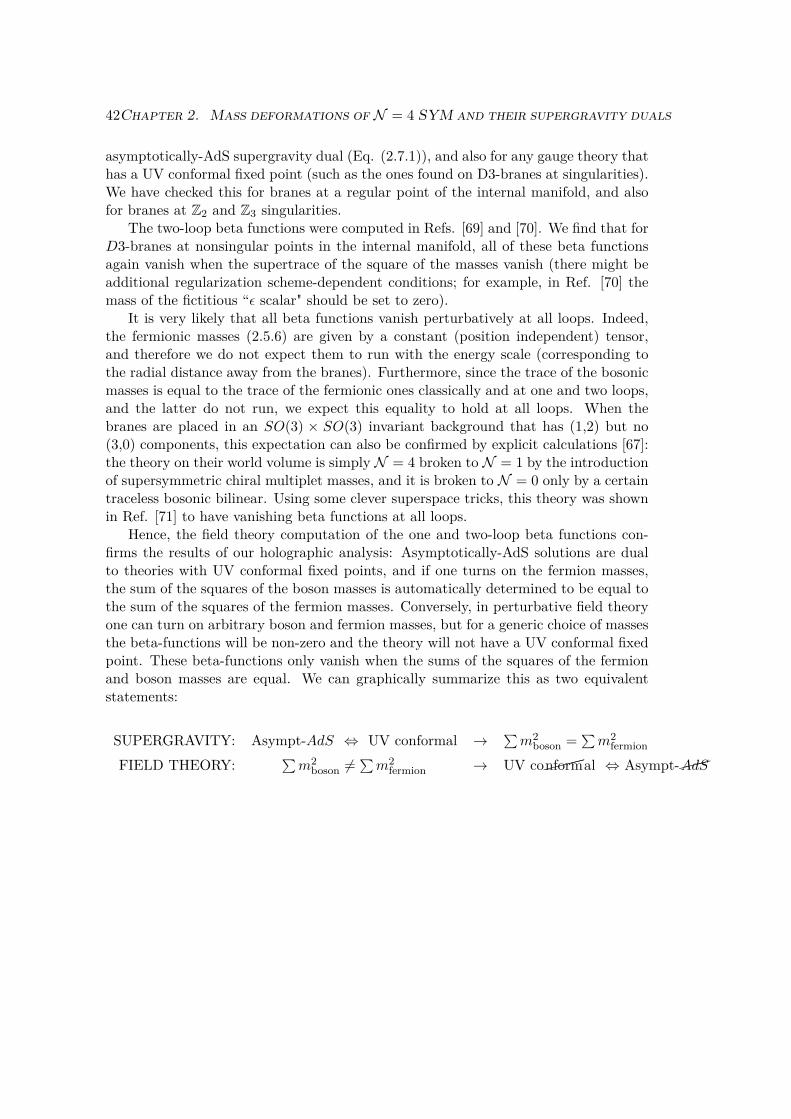
42Chapter 2. Mass deformations of N = 4 SYM and their supergravity duals
asymptotically-AdS supergravity dual (Eq. (2.7.1)), and also for any gauge theory thathas a UV conformal fixed point (such as the ones found on D3-branes at singularities).We have checked this for branes at a regular point of the internal manifold, and alsofor branes at Z2 and Z3 singularities.
The two-loop beta functions were computed in Refs. [69] and [70]. We find that forD3-branes at nonsingular points in the internal manifold, all of these beta functionsagain vanish when the supertrace of the square of the masses vanish (there might beadditional regularization scheme-dependent conditions; for example, in Ref. [70] themass of the fictitious “ε scalar" should be set to zero).
It is very likely that all beta functions vanish perturbatively at all loops. Indeed,the fermionic masses (2.5.6) are given by a constant (position independent) tensor,and therefore we do not expect them to run with the energy scale (corresponding tothe radial distance away from the branes). Furthermore, since the trace of the bosonicmasses is equal to the trace of the fermionic ones classically and at one and two loops,and the latter do not run, we expect this equality to hold at all loops. When thebranes are placed in an SO(3) × SO(3) invariant background that has (1,2) but no(3,0) components, this expectation can also be confirmed by explicit calculations [67]:the theory on their world volume is simply N = 4 broken to N = 1 by the introductionof supersymmetric chiral multiplet masses, and it is broken to N = 0 only by a certaintraceless bosonic bilinear. Using some clever superspace tricks, this theory was shownin Ref. [71] to have vanishing beta functions at all loops.
Hence, the field theory computation of the one and two-loop beta functions con-firms the results of our holographic analysis: Asymptotically-AdS solutions are dualto theories with UV conformal fixed points, and if one turns on the fermion masses,the sum of the squares of the boson masses is automatically determined to be equal tothe sum of the squares of the fermion masses. Conversely, in perturbative field theoryone can turn on arbitrary boson and fermion masses, but for a generic choice of massesthe beta-functions will be non-zero and the theory will not have a UV conformal fixedpoint. These beta-functions only vanish when the sums of the squares of the fermionand boson masses are equal. We can graphically summarize this as two equivalentstatements:
SUPERGRAVITY: Asympt-AdS ⇔ UV conformal → ∑m2
boson = ∑m2
fermion
FIELD THEORY: ∑m2
boson 6=∑m2
fermion → UV conformal ⇔ Asympt-AdS

Chapter 3Supersymmetry and (Generalized) Ge-ometry
As we explained in section 1.4, string theory compactifications that preserve somesupersymmetry can be studied much more easily than non-supersymmetric ones dueto the fact that the supersymmetry equations contain only first derivatives of thespinors while the equations of motion are second order differential equations. In thischapter, we are going to take a closer look to the restrictions imposed on the solutionsby supersymmetry and more specifically, we are going to see how the latter determinesthe geometrical structure of the internal manifold.
Our final goal is to describe the Killing spinor equations ((1.4.5), (1.4.6),(1.4.7)and (1.4.12), (1.4.13),(1.4.14)) in purely geometrical terms. These expressions arecompletely general in the sense that any flux configuration respecting the isometriesof the external space is allowed. Although our goal is to study the geometry in thisgeneral case, it is much easier to develop our tools for this study starting with simplifiedversions of the problem and then generalize them by relaxing our assumptions step bystep.
The structure of this chapter follows the aforementioned generalization procedure.We start in section 3.1 by reviewing the general requirements that are imposed onthe topology and the geometry of the internal manifold due to supersymmetry. Thesimplest cases arise for fluxless compactifications down to four dimensions where theinternal manifold is described by the Calabi-Yau geometry, and five-dimensional com-pactifications with only five-form flux turned on in which case the internal manifold isSasaki-Einstein.
In section 3.2, we make a first step towards the geometrization of the supergravityfluxes by introducing O(d,d)-generalized geometry. At this level of generalization, thefluxes from the NS-NS sector are incorporated in the geometry in the way we explainin subsection 3.2.1. Then, in 3.2.2 we describe how the Killing spinor equations can bewritten in a O(d,d)-generalized geometric way as the integrability conditions of purespinors on the generalized tangent bundle.
On the other hand, fluxes from the R-R sector act as obstruction to the integra-bility of pure spinors and they cannot be given a geometric meaning in the context ofO(d,d)-generalized geometry. One needs to generalize the geometry further and con-
43

44 Chapter 3. Supersymmetry and (Generalized) Geometry
sider structures transforming in representations of the exceptional groups Ed(d) . Therelevant geometry is thus called Exceptional Generalized Geometry (EGG). In section3.3, we introduce the main ideas of this generalization providing more details for theparticular case of E6(6) . In the next chapter, we analyse the supersymmetry condi-tions in the language of EGG and we show how these follow from the Killing spinorequations.
Generalized geometry was introduced by Hitchin and his students [72],[73] in orderto describe complex and symplectic geometry in a unifying framework. It was thenrealized that these are precisely the kind of geometries relevant for string compact-ifications with fluxes [74], [75]1. The original references for Exceptional GeneralizedGeometry are [77] and [78].
3.1 Supersymmetry, topology and geometry
The Killing spinor equations that we encountered in section 1.4 are actually statementsabout the internal manifold with η or χ serving as the expansion coefficients of theten-dimensional supersymmetry parameters in the solution under study (see (1.4.3)and (1.4.9)). Hence, when we write a Killing spinor equation for the internal manifold,it is always implied that such a mode expansion can be made for the ten-dimensionalspinor which is a non-trivial requirement for the internal manifoldM. Having that inmind, we distinguish the superysmmetry constraints in two classes:
• Topological constraints on the manifold. The internal space should have the righttopological properties that allow for the existence of a spinor field (satisfyingcertain reality and chirality conditions) in a well-defined way. More technically,the spinor implies a reduction of the structure group2[79] of the tangent bundleofM.
• Differential constraints on the manifold. Equations (1.4.6) and (1.4.13) actuallydescribe the parallel transport of the internal spinor. This is a statement aboutthe connection defined onM and in technical terms leads to a reduction of theholonomy group3 of the internal space.
Let us now start discussing the simplest case of compactifications of type II super-gravity in the absence of fluxes with (at least) a covariantly constant spinor (1.4.8)on the internal manifold. We will specialize to the case where the internal manifoldis six-dimensional although most of the definitions and statements hold for all even-dimensional manifolds which admit a covariantly constant spinor.
1The deep relation between supersymmetric solutions and generalized geometry can also be seenat the ten-dimensional level [76].
2The structure group is the group of transition functions that are allowed in order to preserve somestructure (or structures) on the overlap of two patches. The existence of well-defined tensors (tensorswhich take a constant value in every patch with a particular choice of frame) reduces the structuregroup from GL(d,R) to a subgroup G of it. We refer to such a strucure as a G-structure.
3The holonomy group is related to the parallel transport of vector (or spinor) around a closed loop.Generically, the new vector differs from the original one by a GL(d,R) element. The group of all suchtransformations is a subgroup of GL(d,R) and is defined as the holonomy group.

3.1. Supersymmetry, topology and geometry 45
From the spinor η, one can construct the following real two-form
ωab = −2iη†Γabη (3.1.1)
which is well-defined onM. The existence of ω reduces the structure group to Sp(6,R).Furthermore, since η is covariantly constant, ω is closed:
dω = 0 (3.1.2)
This actually implies the integrability of ω in the sense that one can define the so-calledDarboux coordinates (qi,pi), i = 1,2,3 such that
ω = dpi ∧ dqi (3.1.3)
In such a case, we say that a symplectic structure is defined onM.The spinor η (and its charge conjugate ηc = C∗η∗) can be also used for the con-
struction of another important three-form:
Ωabc = −2iηc†Γabcη (3.1.4)
Ω is a complex three-form and in order to be well-defined, the structure group shouldbe in SL(3,C). The existence of Ω is related to the existence of an almost complexstructure onM, i.e. a tensor Iab satisfying
IacIcb = −δab (3.1.5)
Moreover, Ω is also closeddΩ = 0 (3.1.6)
implying that I is integrable4 (and hence becomes a complex structure) which actuallymeans that one can define complex coordinates onM. Splitting then the componentsof Ω and ω in holomorphic and anti-holomorphic, one has that that Ω is of type (3,0)and ω of type (1,1) and they satisfy the following compatibility5 condition
ω ∧ Ω = 0 (3.1.7)
The structure group of M then lies in the intersection of the symplectic and thecomplex structure6
SU(3) = Sp(6,R) ∩ SL(3,C) (3.1.8)
Complex manifolds which have a closed real two-form ω which is compatible withthe complex structure are called Kähler manifolds and ω a Kähler form. In our case,we have in addition that Ω is closed and therefore the manifold is Calabi-Yau.
4Actually, the closure of Ω is a stronger condition than the integrability of I. A necessary andsufficient criterion for the latter is the vanishing of the Nijenhuis tensor the components of which aregiven by (NI)abc = Idc∂dI
ab − Idb∂dIac + Iad∂bI
dc − Iad∂cIdb.
5Another equivalent statement would be that the symplectic structure can be obtained from thecomplex structure by lowering an index with the metric.
6The fact that the structure group is SU(3) (instead of U(3)) is related to the fact that the
normalization of Ω is fixed by ωd/2 = (d/2)!2d/2
(−1)d(d/2+1)
4 id/2Ω ∧ Ω.

46 Chapter 3. Supersymmetry and (Generalized) Geometry
Calabi-Yau manifolds are Ricci-flat manifolds and therefore the Einstein equationfor the internal manifold is satisfied in the absence of fluxes. As we mentioned in1.4, the main advantage of compactifications on Calabi-Yau manifolds is the fact theset of harmonic forms7 is well known. Using the so-called Hodge theorem, one canshow that the space of harmonic p-forms is in one-to-one correspondence with thepth-cohomology. Information about the cohomology classes for a Kähler manifolds isencoded in what is known as the Hodge diamond. This is a diamond-like diagramwhich contains in its entries the dimensions of the various (p,q)-cohomology classeswhere p(q) is the number of holomorphic(antiholomorphic) indices for each form. Fora Calabi-Yau 3-fold, the information contained in its Hodge diamond is the following:
• There is 1 one-form (with representative 1), 1 (3,0)-form and 1 (0,3)-form (withrepresentatives Ω and Ω) and 1 (3,3)-form which can be represented by the CYvolume.
• There are h1,1 (1,1)-forms and h2,1 (2,1)-forms as well as another h1,1 (2,2)-formsand h2,1 (1,2)-forms following from the symmetries of the Hodge diamond.
We see that the CY 3-fold is characterized by two numbers of topological nature, h1,1
and h2,1. Given the above and choosing appropriate bases so that certain orthogonal-ity properties are satisfied, one can expand any given form-field and deformations ofthe metric in this basis. One can then perform the dimensional reduction by integrat-ing over the internal manifold in a similar fashion to the torus case, although morecomplicated.
We turn now to compactifications on odd-dimensional manifolds and we will beparticularly interested in the case d = 5. Here, one cannot apply the same ideasthat led to the concept of Calabi-Yau manifolds since one cannot have a complex or asymplectic structure. However, there is an analogous geometrical description which isderived directly from the Killing spinor equation (1.4.16) in a similar fashion that theCalabi-Yau conditions are derived from (1.4.8) which is the Killing spinor equation forCalabi-Yau manifolds.
At first sight, it might seem like (1.4.16) is “destroying” the Calabi-Yau condition(1.4.8). However, it turns out that the most natural way to understand the former isas a special case of the analysis for the latter. To see this, letM be a five-dimensionalinternal manifold and let C(M) be the cone over it8:
ds2C = dr2 + r2ds2
M (3.1.9)
Let us also construct a Weyl spinor θ living on the cone from the spinor χ living onM in the following way:
θ =(χ−iχ
)(3.1.10)
Taking the covariant derivative on the cone, we see that the extra piece of the spinconnection cancels the flux term in (1.4.16) yielding
∇(C)θ = 0 (3.1.11)7A form is harmonic if it is both closed and coclosed. Forms that are harmonic on the internal
manifold are massless if viewed as fields on the external space.8For convenience, we have set m = 1 in (1.4.16).

3.1. Supersymmetry, topology and geometry 47
and therefore the cone is a Calabi-Yau manifold! We are thus naturally led to thefollowing definitions which can be given without involving supersymmetry.
• A manifold is Sasaki if the cone over it is Kähler.
• A manifold is Sasaki-Einstein if the cone over it is Calabi-Yau.
Sasaki-Einstein manifolds are Einstein manifolds (as the name suggests), a propertywhich is inherited from the Ricci-flatness of the Calabi-Yau cone.
As we saw before, the Calabi-Yau conditions can be given either in spinor lan-guage (1.4.8) or in form language (3.1.2),(3.1.6) and (3.1.7). A similar story hap-pens for Sasaki-Einstein (SE) manifolds which are characterized by a triplet of objects(ξ, ωB,ΩB) (or equivalently (σ, ωB,ΩB)) which we are going to define through the coneconstruction.
The Reeb vector ξ is defined through the complex structure on the cone as
ξ = I(r∂r) (3.1.12)
This has a vanishing cone direction ξr = 0 and therefore lies in the Sasaki-Einsteinmanifold. The contact form σ which is defined in the “dual manner”9:
σ = I(r−1dr) (3.1.13)
lies in the SE manifold and satisfies
ιξσ = 1 (3.1.14)
Finally, the two-forms ωB and ΩB for Sasaki-Einstein manifolds can be defined throughthe cone construction as10
ωB = 1r2ω −
1rdr ∧ σ (3.1.15)
andΩB = − i
r3 ιξΩ (3.1.16)
A Sasaki-Einstein manifold can be seen as a fibration over a Kähler-Einstein basedefined by the Reeb vector. Then, ωB becomes a (1,1)-form and ΩB a (2,0)-form withrespect to the complex structure defined on the base. ωB is related to the contactstructure σ through
dσ = 2ωB (3.1.17)
The closure of the Calabi-Yau structures ω and Ω translate to
dωB = 0 (3.1.18)
anddΩB = 3iσ ∧ ΩB (3.1.19)
9Note that in components, there is a minus sign due to the natural action of tensors on forms, i.e.:(A · j)a = −Abajb.
10We are assuming that the holomorphic (3,0)-form of the Calabi-Yau satisfies LξΩ = 3Ω which isalways possible in a non-compact Calabi-Yau.

48 Chapter 3. Supersymmetry and (Generalized) Geometry
while they also satisfy ιξωB = ιξΩB = 0. Finally, the compatibility condition (3.1.7)and the normalization of Ω imply
ωB ∧ ΩB = 0 (3.1.20)
andωB ∧ ωB = 1
2ΩB ∧ ΩB (3.1.21)
3.2 O(d,d) Generalized Geometry
In the previous section, we saw that the main features of Calabi-Yau and Sasaki-Einstein manifolds can be conveniently described using the tools of complex andsymplectic geometry. However, these geometries appeared in rather special cases ofstring theory backgrounds; the fluxless case for compactifications to four-dimensionalMinkowski vacua and flux compactifications but with only special flux configuration(we considered the case where only F5 was non-zero) for AdS5 vacua. In order to studymore general backgrounds, we need to generalize the geometric concepts we use.
3.2.1 Geometrizing the NS-NS degrees of freedomThe starting point of generalized geometry is the extension of the tangent bundle TMof the internal manifold to a generalized tangent bundle E in such a way that theelements of this bundle generate all of the bosonic symmetries of the theory (diffeo-morphisms and gauge transformations). The generalized tangent bundle transforms ina given representation of the corresponding duality group acting on the symmetries.Following the historical path, we start by discussing the O(d,d) generalized geometry,relevant to the NS-NS sector of type II theories compactified on d-dimensional man-ifolds. In section 3.3, we introduce Ed(d) generalized geometry which encodes the fullbosonic sector of type II theories compactified on a (d − 1)-dimensional manifold, orM-theory on a d-dimensional geometry.
The NS-NS sector of type II supergravity contains the metric g(mn), the Kalb-Ramond field B[mn] and the dilaton φ. The symmetries of this theory are diffeomor-phisms generated by vectors k and gauge transformations of the B-field which leave theH = dB invariant and which are parametrized by one-forms λ. The latter correspondsto the restriction of the first transformation in (1.2.5) restricted on the d-dimensionalinternal manifold. The combined action of these symmetries can be thought to begenerated by a single object
V = (k, λ) , k ∈ TM , λ ∈ T ∗M (3.2.1)
on the combined bundle TM⊕ T ∗M. In fact, V is well-defined only in a patch ofM.If there is H-flux, the gauge potential can change in the overlap of two patches by agauge transformation leaving the field strength invariant in a situation similar to theDirac string. In order to construct a global section of the bundle, we need to consider
eBV ≡ (k, λ+ ιkB) (3.2.2)

3.2. O(d,d) Generalized Geometry 49
taking thus into account the non-trivial transformation of the B-field on the overlapof two patches. These generalized vectors belong to the generalized tangent bundle
E ' TM⊕ T ∗M (3.2.3)where the isomorphism is provided by the eB defined above. The structure group ofthis bundle can be reduced from GL(2d) to O(d,d) by observing that there exists aninvariant metric defined by
η(V, V ′) ≡ 12(ιkλ′ + ιk′λ) . (3.2.4)
The symmetries of this metric are:• ka → Aabk
b, λa → Aabλb, where A ∈ GL(d,R) and AcaAcb = δab ,
• ka → ka, λa → λa +Babkb, where B ∈ ∧2T ∗M
• ka → ka + βabλb, λa → λa, where β ∈ ∧2TMAll together, they form the group O(d,d) which corresponds to the T-duality group oftoroidal compactifications that we encountered in section 1.1. The first two of thesesymmetries are related to the fact that the components of metric and the B-field changeon the overlap of two patches and therefore generalized diffeomorphisms parametrizedby V have to take this fact into account. The meaning of the last transformation is moresubtle since there is no “β-field” in the type II supergravity action. For more detailsfor the interpretation of the β- transform in the context of non-geometric backgrounds,the reader is referred to [80],[81],[82],[83],[84],[85] and [86].
It is possible to extend many of the concepts of ordinary differential geometryon TM to analogues on E. The resulting geometry is called Generalized ComplexGeometry (GCG) or O(d,d)-generalized geometry11.
One of the key elements in this construction is the analogue of the Lie derivative.This is the so-called Dorfman derivative along a generalized vector V on anothergeneralized vector V ′12. It expresses the infinitesimal action of the symmetries encodedin V and is given by13
LV V ′ = (Lkk′,Lkλ′ − ιk′dλ) (3.2.5)where L is the ordinary Lie derivative. One can write this in a more O(d,d)-covariantway by embedding the ordinary derivative in a O(d,d)-covariant object through
DM = (∂m, 0) ∈ E∗ (3.2.6)where m = 1,...,d, while M = 1,...,2d. The Dorfman or generalized Lie derivative(3.2.5) takes the form
LV V ′ = (V ·D)V ′ − (D × V )V ′ (3.2.7)where · and × stand respectively for the inner product and the projection to the adjointrepresentation between the vector and dual vector representations14.
11For a more complete introduction to this with a focus on supergravity applications, see [87]. Anice review for generalized complex geometry with applications for D-branes is [88].
12By the Leibniz rule, it can be extended to arbitrary tensors constructed from E and E∗.13Note that V and V ′ now are sections of E and therefore the Dorfman derivative takes into account
the non-triviality of the B-field patching.14Using explicit indices, V ·D = VMDM , (D × V ) = DMV
N |adjoint. In the O(d,d) case, the latteris (D × V )MN = DMV
N − ηNP ηMQDPVQ.

50 Chapter 3. Supersymmetry and (Generalized) Geometry
3.2.2 Supersymmetry in O(d,d) Generalized GeometryIn section 3.1 we explained how the existence and the differential properties of a spinor(or more) on the internal manifold provide topological and geometrical properties ofit. However, this could be done in a clearly geometric way only for rather specialflux configurations; for fluxless backgrounds for d = 6 and only for five-form fluxfor d = 5. For more general backgrounds, the integrability conditions for the relevantstructures fail to be satisfied and one loses the power of geometrical tools that have beendeveloped for Calabi-Yau and Sasaki-Einstein manifolds. Generalized Geometry avoidsthe aforementioned failure by providing geometrical meaning for the fluxes and henceone can obtain integrability conditions for appropriately defined generalized structureswhich have a similar form to the previous ones but describe more general backgrounds.
Let us start with the case of d = 6 which is the relevant one for generalizing theconcept of Calabi-Yau manifolds (or better Calabi-Yau 3-folds). Now, the internalspinor η in appearing in the Killing spinor equations (1.4.5) to (1.4.7) is not any morecovariantly constant and therefore the CY forms ω and Ω are not closed. The firststep therefore is to generalize these objects in their O(d,d) counterparts which willhave now (in general) indefinite rank. These are first built out of two internal spinorsas
Φ± = η1+ ⊗ η
2†± = 1
4
6∑k=0
1k!η
2†± Γa1...akη
1+Γak...a1 (3.2.8)
where in the second equality a Clifford expansion has been performed. One can thenidentify these bispinors with (poly)forms through the Clifford map
6∑k=0
1k!C
(k)a1...akΓa1...ak ←→
6∑k=0
1k!C
(k)a1...akdxa1 ∧ . . . ∧ dxak (3.2.9)
This map allows one to think of Φ± either as (Weyl) spinors of Spin(6,6) or as poly-forms and change easily between the two pictures. As constructed these spinors arepure in the sense that they annihilated by half of the Cliff(6,6) gamma-matrices. In theform language this means that they are annihilated by half of the generalized vectors15
where the (Clifford)16 action of a generalized vector V = (k,λ) on a polyform Φ isdefined by
V · Φ = ιkΦ + λ ∧ Φ (3.2.10)
In order to see how the CY structures embed inside the generalized structures, wehave to set η1 = η2. Then, the pure spinors (3.2.8) reduce to
Φ+ = e−iω, Φ− = −iΩ (3.2.11)
The geometrical significance of the pure spinors Φ± can be seen in a more clear wayif we introduce another piece of terminology. A generalized almost complex structure
15More technically, if the annihilator space of (the space of generalized vectors annihilating) Φ is ofmaximal rank, i.e. is six-dimensional.
16Note that generalized vectors can indeed be interpreted as O(d,d)-gamma matrices since actingon forms they satisfy V,V ′ = 2η(V,V ′).

3.2. O(d,d) Generalized Geometry 51
(GACS)17 is defined as a tensor IAB on the generalized tangent bundle satisfying thefollowing two properties
IACICB = −δAB, ICAηCDIDB = ηAB (3.2.12)
The first of these relations is the direct analogue of to (3.1.5) for the generalized tangentbundle while the second of them expresses the fact that the metric (3.2.4) is hermitianwith respect to this generalized almost complex structure. The existence of a GACSimplies the reduction of the structure group of E from O(6,6) to U(3,3) and it specifiesa splitting of E (or better the complexification of it) into its (±i)-eigenbundles.
The relation of a pure spinor Φ and a GACS I is then established by identifyingthe annihilator space of Φ with the (+i)-eigenbundle of I. Therefore, one obtains aone-to-one correspondence18
pure spinor Φ ↔ I GACS (3.2.13)
We now turn to the integrability conditions for the generalized structures. Thepure spinors Φ± are formal sums of spinor bilinears constructed from the internalspinors η ((3.2.8) and (3.2.9)) and therefore one can use the conditions (1.4.5),(1.4.6)and (1.4.7) to derive differential conditions for Φ±. In the context of N = 1 vacua, thishas been performed in [75] and it corresponds to setting η+
2 = η+2 = 0 in the Killing
spinor equations (see (1.4.3)). We will not provide here the technical details of thiscomputation, but we will state the results and interpret them. The equations one getsfor type IIB are19
(d+H∧)(e2A−φΦ+) = e2A−φ(dA ∧ Φ+ −
i
16eφ+A ?6 FRR
)(3.2.14)
and(d+H∧)(e2A−φΦ−) = 0 (3.2.15)
where we have grouped together the following combination of R-R fluxes
FRR = F1 − F3 + F5 (3.2.16)
The norms of the Spin(6,6) spinors satisfy
|Φ±| = eA (3.2.17)
Let us focus on the second of the two differential conditions (3.2.15) which seemsto attribute integrability properties to the structure Φ−. From the left-hand side, wethat the NS-NS three-form flux H enters the geometry by providing a twisting for theexterior derivative:
dH = d+H∧ (3.2.18)17In string theory, the generalized almost complex structure appears naturally from the worldsheet
point of view [89].18There is a subtlety here since the one-to-one correspondence is modulo an overall factor which is
related to the dilaton and the warp factor in supergravity applications. However, we will not be veryprecise with this factor in the context of O(d,d)-Generalized Geometry.
19Here the H-twisting appears with a different sign than in [75] due to the different conventions weuse.

52 Chapter 3. Supersymmetry and (Generalized) Geometry
Perhaps, we can make the geometric picture more clear by observing that e−BdeB = dHand defining the dressed pure spinors
ΦD = eBΦ (3.2.19)
where the action of the exponential on forms is given by (1.2.4). Neglecting for themoment the scaling factor e2A−φ, (3.2.15) becomes
dΦD− = 0 (3.2.20)
But this is very similar to the Calabi-Yau integrability condition (3.1.6). In fact,the closure of ΦD
− implies that the GACS related to it through (3.2.13) is integrable20
becoming now a generalized complex structure. According to the so-called GeneralizedDarboux Theorem[73], the existence of a generalized complex structure on a manifoldimplies that locally the manifold is equivalent to the product Ck×Rd−2k
Sp where Rd−2kSp is
the standard symplectic space. Therefore, a generalized complex manifold interpolatesbetween a complex and symplectic manifold. The integer k ≤ d/2 is called the rankand is allowed to jump over certain points or planes. Manifolds which admit a purespinor Φ that is closed dΦ = 0 were called in [72] Generalized Calabi-Yau.
Let us now return back to the differential condition (3.2.15) or rather its dressedversion (3.2.20). The eB action (3.2.19) is inherited from the corresponding dressingof generalized vectors (3.2.2) and therefore it is natural to appear in the integrabilityconditions. The scaling factor in (3.2.15) is related on the one hand to the normaliza-tion of the internal spinors (see (3.2.17) or (4.2.4) for the five-dimensional case) andon the other hand to an additional R+ action on the generalized tangent bundle whichwe have neglected here (see [87] for details).
We therefore see that, according to our previous discussion, four-dimensional vacuaN = 1 vacua of type IIB supergravity with generic fluxes are H-twisted generalizedCalabi-Yau manifolds. This means in particular that there is an (integrable) gener-alized complex structure on the “twisted” generalized tangent bundle spanned by thetwisted generalized vectors (3.2.2).
Moving now to the other differential condition for the pure spinor Φ+, we see thatits integrability is obstructed from the presence of R-R fluxes through the combinationFRR. This means that the GACS related to the pure spinor Φ+ is not integrable. How-ever, this is rather expected since, as we have already explained, in O(d,d)-generalizedgeometry only the NS-NS sector of type II supergravity is geometrized. In reference[90] where N = 2 vacua were studied with NS-NS fluxes only, both pure spinors wereshown to be twisted closed dHΦ± = 0. The inclusion of the R-R fluxes in the geometryrequires a further generalization to which we turn in the next section.
Before closing this section, let us briefly explain how O(d,d)-generalized geome-try works for compactifications of type II theory down to AdS5 (in this case O(5,5)-generalized geometry). The extension of the tangent bundle and the discussion of thesymmetries for the metric η proceeds in exactly the same way as for the six-dimensionalcase. However, in odd dimensions one does not have a generalized almost complex
20Actually, the integrability of a GACS is a weaker condition than the closure of the correspondingpure spinor. A GACS is integrable if there exists a generalized vector V such that the pure spinor Φassociated with the GACS satisfies dΦ = V · Φ.

3.3. Exceptional Generalized Geometry 53
structure and therefore the one-to-one correspondence between a GACS and an O(5,5)pure spinor is not present here. Nevertheless, O(5,5) pure spinors are well-defined andone can derive the differential conditions they satisfy from the Killing spinor equationsfor the internal manifold. We will not get into the details of this analysis, but let usmention some basic facts. The differential conditions have the schematic form[91]21
dHΦ = dA ∧ Φ +mΦ + FRR (3.2.21)
where some terms may be absent depending on the precise form of the bispinor con-sidered. We see that, similarly to the analysis for Mink4 vacua, the R-R fluxes actgenerically as an obstruction for the integrability of Φ and there is also the “peculiar”term dA ∧ Φ on the right-hand side. Furthermore, the AdS5 mass parameter m alsoappears on the right-hand side in a term proportional to Φ. We will see in chapter 4that in exceptional generalized geometry, m is embedded in an SU(2) vector λa whichbreaks the R-symmetry of the theory SU(2)R → U(1)R and there is no term like dA∧Φ(it has been incorporated in the geometry).
The fact that the supersymmetry conditions have a similar form in O(6,6) andO(5,5)-generalized geometry gives us evidence that they could be described in a uni-fied form for various dimensions. It turns out that is true in exceptional generalizedgeometry where the supersymmetry conditions have exactly the same form for variousdimensions and the only thing that changes is the group theory formulae.22.
3.3 Exceptional Generalized Geometry
The usefulness of generalized geometry in describing supersymmetric vacua in stringcompactifications, in the way we described in the previous section, is the fact that thestructure group of the generalized tangent bundle at each point inM, namely O(d,d)coincides with the T-duality group of the massless sector of string theory. T-dualitytransforms the NS-NS sector and the R-R sector separately, i.e. does not mix them.However, the NS-NS and R-R sectors are the bosonic parts of the supersymmetric fullstring theory and we expect further symmetries mixing them to hold.
In order to include the gauge transformations of the R-R fields, or to do a general-ized geometry for M-theory, one needs to extend the tangent bundle even further. Notsurprisingly, the appropriate generalized bundle should transform covariantly underthe group Ed(d) [77, 78], which is the U-duality group of the massless sector of type IIstring theory (M-theory) when compactified on a d − 1 (d) dimensional manifold. Inthe concrete applications in chapter 4, we will deal with compactifications of type IIBand M-theory down to five dimensions, and the relevant group is therefore E6(6) . Thisextended version of generalized geometry is called Exceptional Generalized Geometry[93, 94]. In the following, we will introduce the main ideas of Exceptional GeneralizedGeometry for the type IIB case, and then we will present the analogous concepts forM-theory compactifications.
21The supersymmetry conditions for AdS4 vacua were derived in [92] and they have a similar formto (3.2.21).
22In the next chapter we will study just AdS5 vacua where the relevant group is E6(6) , but theanalysis is similar for AdS4 vacua with the U-duality group being E7(7).

54 Chapter 3. Supersymmetry and (Generalized) Geometry
The generalized tangent bundle for type IIB decomposes as follows
E ' TM⊕ (T ∗M⊕ T ∗M)⊕ ∧3T ∗M⊕ (∧5T ∗M⊕∧5T ∗M) (3.3.1)
where the additional components T ∗M , ∧3T ∗M and the two copies of ∧5T ∗M corre-spond to the gauge transformations of C2, C4, C6 and B6, the dual of B2 (one can alsounderstand this in terms of the charges of the theory, namely D1, D3, D5 and NS5-brane charges respectively). In the above expression, we have grouped together termsthat transform as doublets under the SL(2,R) symmetry of type IIB supergravitywhich we encountered in section 1.2.
The isomorphism implied in (3.3.1) is given by an element eµ ∈ E6(6) , µ ∈ e6(6)which can be constructed from the gauge fields of the theory in such way that thegeneralized vectors are well-defined in the overlap of two patches. This is in directanalogy with the O(d,d) case where the only non-trivial gauge field is the B-field. Theexpression for µ in our case is given below in (3.3.6).
One can also here embed the derivative in a covariant object in E∗, such that itsnon-zero components are on T ∗M. The Dorfman derivative takes the same form as inthe O(d,d) case, namely (3.2.7). For its expression in terms of the GL(5) decompositionof E in (3.3.1), namely the analogue of (3.2.5), see [93].
Finally, let us mention that a complete treatment of both O(d,d) and Ed(d) gener-alized geometry also includes the geometrization of the so-called trombone symmetry(see [93] for details). This is an additional R+ symmetry which exists in warpedcompactifications of M-theory and can be understood as a combination of the scalingsymmetry in the eleven-dimensional theory (1.3.9) (and therefore is inherited also intype II) and constant shifts of the warp factor in the compactified theory. In order toincorporate the action of this symmetry for the supersymmetry conditions in chapter(4), we rescale appropriately our structures (see (4.1.10) below) where the appearanceof the dilaton in the type IIB case reflects the fact that the dilaton can be interpretedas a contribution to the warp factor in an M-theory set-up.
Particular case of E6(6)
Let us now specialize to the case of E6(6) . The generalized tangent bundle E transformsin the fundamental 27 representation, whose decomposition is given in (3.3.1). In termsof representations of GL(5)× SL(2)23 this is
27 = (5,1)⊕ (5,2)⊕ (10,1)⊕ (1,2) . (3.3.2)
It will actually turn out to be convenient to use the SL(6) × SL(2) decomposition,where the two SL(2) singlets are combined into a two-vector, while the two SL(2)doublets are combined into a doublet of forms. Under SL(6)×SL(2) the fundamental(anti-fundamental) representation V (Z) of E6(6) therefore decomposes as
27 = (6,2) + (15,1), V = (V ia, V
ab) (3.3.3a)
27 = (6,2) + (15,1), Z = (Zai, Zab) (3.3.3b)23For details in the representations of E6(6) see appendix C.

3.3. Exceptional Generalized Geometry 55
where a,b,c, . . . run from 1 to 6 and i,j,k, . . . from 1 to 2.The derivative embeds naturally in the anti-fundamental representation as24
Dim = Di
6 = Dmn = 0, Dm6 = e2φ/3∂m (3.3.4)
where we use m,n, . . . for the coordinate indices on the internal manifold.The adjoint representation splits under SL(6)× SL(2) as
78 = (35,1) + (1,3) + (20,2), µ = (µab,µij , µiabc) . (3.3.5)
In our conventions, the dilaton and gauge fields embed in this representation in thefollowing way
µ1mn6 = eφCmn (3.3.6a)
µ2mn6 = Bmn (3.3.6b)
µmn = −φ6 δmn (3.3.6c)
µ66 = 5φ
6 (3.3.6d)
µn6 = −eφ(∗C4)n (3.3.6e)
µij =(−(φ/2) eφC0
0 (φ/2)
)(3.3.6f)
while the other components of µ vanish25. Note that the the gauge fields from the R-Rsector carry an eφ factor.
E6(6) for M-theory
We now turn to compactifications of eleven-dimensional supergravity down to AdS5and outline the M-theory counterpart of the of the above construction. The situationis similar to the type IIB case since the group of global symmetries remains the same,namely E6(6) . However, the analogous formulae are more transparent since M-theorycombines the degrees of freedom in a more compact form, avoiding thus the compli-cations due to the GL(5) ⊂ SL(6) embedding. In particular, the generalized tangentbundle is decomposed in this case as
E ' TM⊕∧2T ∗M⊕∧5T ∗M (3.3.7)
where the internal manifold M is now six-dimensional and the various terms corre-spond to momenta, M2- and M5-brane charges respectively. The latter can be dualizedto a vector, and together with the first piece they form the (6,2) piece in the splitof the fundamental 27 representation under SL(6) × SL(2) given in (3.3.3). The
24The reason for the additional factor of e2φ/3 is related to the rescaling of the bispinors which willbe introduced later, see (4.1.10).
25These other components of µ could have non-vanishing values in a different U-duality frame.

56 Chapter 3. Supersymmetry and (Generalized) Geometry
derivative is embedded in one of the two components of this doublet appearing in theanti-fundamental representation26
D2a = ∇a, D1
a = Dab = 0 . (3.3.8)
The decomposition of the adjoint representation is given in (3.3.5), and the three-formgauge field C embeds in µ as
µ1abc = −(?C)abc (3.3.9a)
µ2abc = µij = µab = 0. (3.3.9b)
We therefore see that for both type IIB and M-theory, the effect of the gauge potentialscan be incorporated in the twisting of the generalized tangent bundle by appropriatelyembedding them in an adjoint element eµ of E6(6) . This is similar to the dressing ofpure spinors (3.2.19) by the NS-NS gauge potential eB in O(d,d)-generalized geometrywhere the structure Φ was constructed as a bispinor in (3.2.8). In the next chapter,we will explore compactifications of type IIB and M-theory down to AdS5 preservingeight supercharges with generic fluxes. We will show that one can construct appropri-ate bispinors K and Ja as the generalization of the pure spinors Φ. We will then provethat the dressed objects K = eµK and Ja = eµJa need to satisfy certain integrabil-ity conditions which will be the analogues of the closure of the dressed pure spinors(3.2.20).
26Note that here D does not carry a rescaling factor in contrast to the type IIB case.

Chapter 4
Generalized Geometric vacua with eightsupercharges
The analysis of the previous chapter revealed that in order to incorporate the effect offluxes in geometric structures, one needs to extend the tangent bundle of the internalmanifold appropriately to its generalized version in order to include the charges presentin the theory (momenta, NS-brane and D-brane charges). In the case of O(d,d)-generalized geometry, the generalization of the tangent bundle includes only momentaand NS-brane charges; the latter corresponding to the gauge transformations of theB-field. Therefore, only the NS-NS sector is geometrized.
In this chapter, we will show that in exceptional generalized geometry we are ableto describe the general case (AdS5 vacua with generic fluxes preserving eight super-charges) in a purely geometric way. Specifically, we will write the Killing spinor equa-tions relevant for AdS5 compactifications purely in terms of the geometric structuresK = eµK and Ja = eµJa defined in the previous chapter which live in representa-tions of the corresponding exceptional group. Here, µ contains all the gauge potentials(both from NS-NS and R-R sector, see (3.3.6)) and K and Ja can be constructedas bispinors of the internal spinors. We perform the analysis for both type IIB andM-theory compactifications.
We proceed as follows. In section 4.1 we introduce concretely the exceptionalstructures K and Ja focusing on the type IIB case. In subsection 4.1.1 we describe thecompatibility conditions they should satisfy as a result of their group theory propertieswhile in subsection 4.1.2 we give the integrability properties they should satisfy. Section(4.2) is devoted to the proof of the integrability conditions for the structures K andJa which are constructed as bispinors. In section 4.3, we repeat the analysis for theM-theory case. Intermediate results which we make use of in the analysis are provedin section 4.4. Two key elements in the statement and the proof of the integrabilityconditions are the moment map for Ja and the Dorfman derivative along K. Theirexplicit calculation is given in sections 4.5 and 4.6 respectively. Appendix C containsthe necessary group theory formulae to derive the results in this chapter.
57

58 Chapter 4. Generalized Geometric vacua with eight supercharges
4.1 Supersymmetry in Exceptional Generlaized Geometry
4.1.1 Backgrounds with eight superchargesIn the end of the previous chapter we mentioned briefly how the supergravity degreesof freedom can be packed into generalized geometric objects which belong to repre-sentations of the corresponding duality group. In this section, we focus on the caseof backgrounds that have eight supercharges off-shell, and in the next subsection weshow how the on-shell restriction (i.e., the requirement that the background preservesthe eight supercharges) is written in the language of exceptional generalized geometry.
As we explained in section 3.1, backgrounds with off-shell supersymmetry are char-acterized in ordinary geometry by the existence of well-defined spinors, or in otherwords a reduction of the structure group of the tangent bundle from SO(d) to sub-groups of it singled out by the fact that they leave the well-defined spinors invariant.This means that the metric degrees of freedom can be encoded in objects that are in-variant under the structure group, built out of bilinears of the spinors. For the familiarcase of SU(d/2) structures (like the case of Calabi-Yau), these objects are the Kähler2-form ω and the holomorphic d/2-form Ω, satisfying certain compatibility conditions1.
On-shell supersymmetry imposes differential conditions on the spinors, which aretranslated into differential conditions on the bilinears of spinors. In the absence offluxes, the supersymmetric solutions involve an external Minkowski space, and thedifferential conditions lead to integrable structures on the internal space. In the case ofM-theory compactifications down to five dimensions preserving eight supercharges, theinternal manifold has to be Calabi-Yau, namely the Kähler 2-form and the holomorphic3-form are closed.
Compactifications to AdS require on one hand some flux to support the curvature,and on the other hand the integrability conditions are weaker (they are usually referredto as weakly integrability conditions)2. The simplest example of compactifications toAdS5 is that of type IIB, where the curvature is fully provided by the 5-form flux,and the internal space is Sasaki-Einstein (the simplest case being S5). In section3.1 we saw that Sasaki-Einstein manifolds are U(1)-fibrations over a Kähler-Einsteinbase (defined by a Kähler 2-form ωB and a holomorphic 2-form ΩB satisfying thecompatibility condition) and a contact structure σ, satisfying3
dσ = 2mωB, dΩB = 3imσ ∧ ΩB (4.1.1)
where m is at the same time the curvature of the internal space (more precisely, theEinstein condition is Rmn = 4m2gmn), that of AdS5, and give also the units of five-form flux. The integrability conditions on the structures for more general solutionswere obtained in [24].
In M-theory there is no such a simple AdS5 solution. The most well known solutionis that of Maldacena and Nuñez [26], corresponding to the near horizon limit of M5-
1These were given in section 3.1 and we repeat them here for convenience:ω ∧ Ω = 0, , ωd/2 = (d/2)!
2d/2(−1)
d(d/2+1)4 id/2Ω ∧ Ω.
2For full integrability all torsion classes are zero, while for weak integrability there is a torsion in asinglet representation of the structure group, proportional to the curvature of AdS.
3Here, we have restored the AdS5 curvature m which we had set to 1 in chapter 3.

4.1. Supersymmetry in Exceptional Generlaized Geometry 59
branes wrapped on holomorphic cycles of a Calabi-Yau 3-fold. More general solutionsare studied in [95], and correspond topologically to fibrations of a two-sphere over aKähler-Einstein base.
The effective five-dimensional gauged supergravity encodes the deformations of thebackground. When there is a G-structure, the moduli space of metric deformations isgiven by the deformations of the structures. Together with the moduli coming fromthe B-field and the R-R fields, they form, in the case of N = 2 gauged supergravity,the hypermultiplets and vector multiplets of the effective theory.
In the generalized geometric language, metric degrees of freedom can also be en-coded in bilinears of spinors (this time transforming under the the compact subgroupof the duality group, namely USp(8) for the case of E6(6) ), and furthermore these canbe combined with the degrees of freedom of the gauge fields such that the correspond-ing objects (called generalized structures4) transform in given representations of theEd(d) group. For eight supercharges in five dimensions the relevant generalized struc-tures form a pair of objects (K,Ja), first introduced in [9]. In the next section we aregoing to give their explicit form, but for the moment let us explain their geometricalmeaning.
The structure K transforms in the fundamental representation of E6(6) and it isa singlet under the SU(2) R-symmetry group of the relevant effective supergravitytheory. If K was to be built just as a bispinor (we will call that object K, its explicitexpression is given in (4.2.14)), then it would be a section of the right-hand side of(3.3.1) and it would not capture the non-trivial structure of the flux configuration onthe internal manifold. Therefore, the proper generalized vector which transforms as asection of E is the dressed one
K = eµK . (4.1.2)This structure was called the V-structure (vector-multiplet structure) in [10] since itparametrizes the scalar fields of the vector multiplets in the effective theory.
The other algebraic structure, or rather an SU(2)R triplet of structures, describingthe hypermultiplets (and thus called H-structure in [10]) is Ja, a = 1,2,3. It transformsin the adjoint of E6(6). As for K, we need the dressed object
Ja = eµJae−µ = eJµ,·KJa (4.1.3)
where we are using J·, ·K to denote the e6(6) adjoint action. These are normalized as5
Tr(Ja,Jb) = 8ρ2δab (4.1.4)
where ρ will be related to the warp factor, and satisfy the SU(2) algebra
JJa,JbK = (4iρ)εabcJc . (4.1.5)
As in Calabi-Yau compactifications where ω and Ω have to satisfy compatibilityconditions to define a proper Calabi-Yau structure (see footnote 1), similar require-ments apply here, and read
JaK = 0 , c(K,K,K) = 6ρ3 (4.1.6)4In the case of O(d,d) generalized geometry these are Spin(d,d) pure spinors.5We use the notation Tr(·,·) to denote the Killing form for e6(6).

60 Chapter 4. Generalized Geometric vacua with eight supercharges
where in the first expression we mean the adjoint action of J on K, and in the secondone c is the cubic invariant of E6(6) . Since the above expressions are E6(6) -covariant,they have exactly the same form if we replace (K,Ja) with their dressed version (K,Ja).
4.1.2 Supersymmetry conditions
In the previous section we have introduced the generalized structures defining thebackgrounds with eight supercharges off-shell, namely those that allow to define a five-dimensional (gauged) supergravity upon compactification. Here we discuss the inte-grability conditions that these backgrounds need to satisfy in order to preserve all eightsupersymmetries leading to an AdS5 geometry on the external space. The supersym-metry conditions were originally introduced in [11], and the relevant backgrounds called“exceptional Sasaki-Einstein” (the simplest case corresponding to Sasaki-Einstein man-ifolds). Here we will write the supersymmetry conditions in a slightly different way,and in section 4.2 we will use the fact that they are independent of the (generalized)connection6 to choose a convenient one to verify them directly from the ten-dimensionalsupersymmetry conditions.
Compactifications to warped AdS5 require, both in M-theory and in type IIB7
DJa + κ εabcTr(Jb, DJc) = λac(K,K, ·) (4.1.7)
LKK = 0 (4.1.8)
LK Ja = 3i2 εabcλbJc (4.1.9)
These equations involve the rescaled bispinors, which for type IIB are (the analogueexpressions for M-theory are given in (4.3.1))
K = e−2φ/3K , Ja = e2A−2φJa , (4.1.10)
where A is the warp factor and φ the dilaton. D is the derivative defined in (3.3.4),whose explicit index we have omitted, and corresponds to the direction missing in thecubic invariant8. The coefficient κ is related to the normalization of the structures andis given by
1κ
= i‖Ja‖ ≡ i√
8Tr(Ja,Ja) (4.1.11)
and for type IIB is9
κ = − i
4√
2e−3A+2φ. (4.1.12)
Finally, λa are a triplet of constants related to the AdS5 cosmological constant m by
λ1 = λ2 = 0, λ3 = −2im . (4.1.13)6See [93] for details.7In our conventions, (4.1.9) has a different sign in M-theory, see (4.3.3).8To write this index explicitly we substitute D → DM , c(K,K, ·)→ cMNP K
NKP .9Note that κ accounts for both the normalization of the internal spinors (see (4.2.4) below) and
the rescalings (4.1.10) as can be seen by writing it as κ = (8iρe2A−2φ)−1.

4.2. From Killing spinor equations to Exceptional Sasaki Einstein conditions61
Let us explain very briefly the meaning of these equations. For more details, see[10, 11]. The first equation which one can write in terms of the Dorfman derivativealong a generic generalized vector,10 implies that the moment map for the actionof a generalized diffeomorphism along V takes a fixed value that involves the vectormultiplet structure and the SU(2)R breaking parameters λa (AdS5 vacua only preservea U(1)R ∈ SU(2)R [12, 96]), given by λaJa. The second and third equation imply thatK is a generalized Killing vector of the background. Indeed, (4.1.8) implies that itleaves K invariant, while (4.1.9) shows that the generalized diffeomorphism along Kamounts to an SU(2)R rotation of the Ja. This rotation does not affect the generalizedmetric which encodes all the bosonic degrees of freedom. Thus, the generalized vectorK was called “generalized Reeb vector” of the exceptional Sasaki-Einstein geometry.
As shown in [11], these conditions imply that these backgrounds are generalizedEinstein, as the generalized Ricci tensor is proportional to the generalized metric.
We can compare these to the conditions coming from the five dimensional gaugedsupergravity [12]. More specifically, (4.1.9) corresponds to the hyperini variation,(4.1.8) corresponds to the gaugini, while (4.1.7) corresponds to a combination of thegravitini and the gaugini.
In the next section, we will give more details of the construction of H-and V struc-tures in terms of internal spinors, and we show by an explicit calculation that AdS5compactifications preserving eight supercharges require conditions (4.1.7)-(4.1.9).
4.2 From Killing spinor equations to Exceptional Sasaki Ein-stein conditions
In this section we show that supersymmetry requires the integrability conditions (4.1.7)-(4.1.9).
4.2.1 The Reeb vectorLet us state again the basic conditions which we will require. We are interested insolutions of type IIB supergravity which
• respect the isometry group SO(4,2) of AdS5 and
• preserve 1/4 of the original supersymmetry, i.e. 8 supercharges.
According to the former condition, the ten-dimensional metric is written as (1.4.1)where gµν(x) is now the metric of AdS5 and gmn(y) is the metric of the internalmanifold, while the fluxes are of the form given in (1.4.11) so that they respect thedemocratic constraint (1.2.8) and where F(n) is purely an internal piece.
We start with the supersymmetry transformations of type IIB supergravity for thegravitino and the dilatino. These are given (in the democratic formulation) by (1.2.10)and (1.2.10) respectively.
10The expression is as follows
κ εabcTrJJb,LV JcK = λac(K,K, V ) .

62 Chapter 4. Generalized Geometric vacua with eight supercharges
The ansatz (1.4.9) gives the decomposition of the type IIB spinors (1.2.9) in termsof the external spinor ψ and the internal spinors χi. The spinor ψ is a Killing spinorfor AdS5 and therefore is required to satisfy (1.4.10) which involves the AdS5 massparameter m. The latter enters the Killing spinor equations for the internal spinors χithrough the external component of the gravitino variation (1.2.10).
Combining the above information, the ten-dimensional Killing spinor equationstranslate into the conditions (1.4.12), (1.4.13) and (1.4.14). These equations containall the information we need to derive the integrability conditions and we repeat themhere for convenience:[
m− eA(/∂A)Γ6Γ7 + ieφ+A
4((/F 1 + /F 5)Γ6 − /F 3
)](χ1χ2
)= 0 (4.2.1)
[∇m −
14/HmΓ6 + i
eφ
8(/F 1 + /F 5 − /F 3Γ6
)ΓmΓ(7)
](χ1χ2
)= 0 (4.2.2)
[(/∂φ)Γ6Γ(7) + 1
2/HΓ7 −
ieφ
2(2/F 1Γ6 − /F 3
)](χ1χ2
)= 0 (4.2.3)
Now, let us mention some generic properties of IIB flux compactifications down toAdS5 which are implied by the supersymmetry requirements. Although these state-ments can be proved without any reference to generalized geometry (as in [24]), we willpostpone their proof until section 4.4.1 to see how nicely this formalism incorporatesthem. Here, we just state them.
The first property has to do with the norms of the internal spinors. From (4.4.8),we see that the two internal spinors have equal norms and from (4.4.11) that they scaleas eA:11
χ†1χ1 = χ†2χ2 ≡ ρ = eA√2
(4.2.4)
Moreover, (4.4.9) expresses the following orthogonality property
χ†1χ2 + χ†2χ1 = 0 (4.2.5)
An important consequence of the supersymmetry conditions which will be crucialfor the geometrical characterization ofM is the existence of an isometry parametrizedby a vector ξ [24], the so-called Reeb vector12. The components of ξ can be constructedfrom spinor bilinears as
ξm = 1√2
(χ†1γmχ1 + χ†2γmχ2) (4.2.6)
Actually, it turns out (see section 4.4.1) that ξ generates a symmetry of the full bosonicsector of the theory:
Lξg,A, φ,H, F1, F3, F5 = 0. (4.2.7)11Note that the ρ defined here is the same as the one appearing in the normalization condition ofJ , Eq. (4.1.4).
12In the context of AdS/CFT, this isometry corresponds in the dual picture to the surviving R-symmetry of the N = 1 gauge theory.

4.2. From Killing spinor equations to Exceptional Sasaki Einstein conditions63
Using this, we can easily see that the Lie derivatives Lξχi of the spinors satisfy the sameequations (1.4.12) - (1.4.14) as the spinors themselves13 and so they are proportionalto them which means that they have definite charge. This charge is computed inappendix 4.4.1. From (4.4.31) we have
Lξχi = 3im2 χi (4.2.8)
These conditions are very useful in proving the integrability conditions in the nextsection.
4.2.2 The H and V structures as bispinorsLet us now construct the H and V structures from the internal spinors, as appropriateE6(6) objects. For this, it is useful to decompose the group in its maximal compactsubgroup USp(8) .14
The fundamental 27 (anti-fundamental 27 ) representation is undecomposable, andcorresponds to an antisymmetric 8×8 matrix V αβ (Zαβ) which is traceless with respectto the symplectic form Cαβ of USp(8)
27 , V = V αβ , such that VαβCαβ = 0 (4.2.9)
The adjoint 78 representation corresponds to a symmetric 8 × 8 matrix and a fullyantisymmetric rank 4 tensor
78 = 36 + 42, µ = (µαβ, µαβγδ) (4.2.10)
The internal spinors (χ1,χ2) which are sections of Spin(5) ∼= USp(4), are combinedinto the following USp(8) spinors
θ1 =(χ1χ2
), θ2 =
(χc1χc2
). (4.2.11)
In terms of the USp(8) spinors θi, the normalization condition (4.2.4) implies
θ∗αi θj,α = 2ρ δij . (4.2.12)
Now, one can define the H and V structures as bispinors in a natural way. Thetriplet of H structures Ja are defined as
(Ja) βα = (σa)ijθi,αθ?βj (4.2.13)where σa = (σ1, σ2, σ3) are the Pauli matrices. Note that Ja have components only inthe 36 piece of the 78.
For the V structure, we have
Kαβ = J αβ0 − 18C
αβCδγJ γδ0 , with (J0) βα = δijθi,αθ?βj (4.2.14)
13Here, note that the existence of the isometry is crucial for the Lie derivative to commute with thecovariant one.
14Here, we just present some basic facts. More details are given in appendix C.

64 Chapter 4. Generalized Geometric vacua with eight supercharges
where Cαβ is the charge conjugation matrix, which in our conventions is the symplecticform of USp(8) . Note that K is traceless by construction. From now on, we will dropthe USp(8) indices α, β in K, J .
The su(2) algebra of the structures Ja, Eq. (4.1.5), follows from the orthogonalityand normalization of the spinors (4.2.12). Similarly we have
J 2a = J 2
0 = 2ρJ0 (4.2.15a)
J0Ja = JaJ0 = 2ρJa (4.2.15b)
where ρ can also be related to the trace part of J0, namely
ρ = 14Tr[J0] (4.2.16)
The fact that Ja and J0 commute translates in E6(6) language (by using (C.2.4))into the compatibility condition (4.1.6).
In the following, it will turn out useful to have explicitly the GL(5)× SL(2) com-ponents of K and Ja. For the former, using the decomposition of the 27 representationgiven in (3.3.2), we have:
K = [ξ, (ζ, ζ7), V, (R,R7)] . (4.2.17)
These can be organized in terms of a Clifford expansion as
K = 12√
2
[iξmΓm67 + ζmΓm + iζ7
mΓm7 + i
2VmnΓmn7]
(4.2.18)
where the various components can be obtained by taking appropriate traces with K15. In terms of bilinears involving the internal spinors χ1 and χ2 these components are
ζm = 1√2
(χ†1γmχ2 + χ†2γmχ1)
ζm7 = 1√2
(−χ†1γmχ1 + χ†2γmχ2)
ξm = 1√2
(χ†1γmχ1 + χ†2γmχ2) (4.2.19)
V mn = 1√2
(χ†1γmnχ2 − χ†2γmnχ1)
R = 1√2
(χ†1χ1 − χ†2χ2)
R7 = 1√2
(χ†1χ2 + χ†2χ1)
Note the absence of R and R7 in the expansion (4.2.18). This is because these vanishas a consequence of the supersymmetry conditions that impose the two internal spinorsto be orthogonal and have equal norm (see (4.2.4), (4.2.5)). Moreover, note that the
15For example, ξm = 12√
2Tr[KΓm67].

4.2. From Killing spinor equations to Exceptional Sasaki Einstein conditions65
vector component ξ of K appearing in the above expression is the Reeb vector givenin (4.2.6).
For the particular case of Sasaki-Einstein manifolds, where χ2 = iχ1, also theone-forms ζ and ζ7 are zero, while the two-form V corresponds to ∗(σ ∧ ωB).16 Theholomorphic 2-form of the base ΩB is instead embedded in Ja, to which we now turn.
The triplet Ja is in the 36 representation of USp(8) , which decomposes underGL(5)× SL(2) as
36 = (5,1) + (10,1) + (1,1) + (10,2) . (4.2.20)
The Clifford expansion of Ja is 17
Ja = −18[Jm6a Γm6 + 1
2Jmna Γmn − J 7
a Γ7 + 12J
mn6a Γmn6 + 1
6Jmnpa Γmnp
](4.2.21)
where each piece is given by the first terms in (C.3.5).In particular, one can identify in the expansion (4.2.21) all possible spinor bilinears
with non-zero charge under ξ18
Jm6+ = 4χT1 γmχ2
Jmn+ = −2(χT1 γmnχ1 + χT2 γmnχ2)
Jmn6+ = −2(χT1 γmnχ1 − χT2 γmnχ2) (4.2.22)Jmnp+ = −4χT1 γmnpχ2
J 7+ = 4iχT1 χ2
where we have definedJ± = J1 ± iJ2 . (4.2.23)
The components of J− have exactly the same form with the replacement χi → χci andan overall minus sign in the above expressions.19 On the other hand, J3 is neutralsince it is constructed from two oppositely charged spinors (χ and χ†). The explicitexpressions for the related bilinears are
Jm63 = 2(−χ†1γmχ2 + χ†2γ
mχ1)Jmn3 = 2(χ†1γmnχ1 + χ†2γ
mnχ2)Jmn6
3 = 2(χ†1γmnχ1 − χ†2γmnχ2) (4.2.24)
Jmnp3 = 2(χ†1γmnpχ2 + χ†2γmnpχ1)
J 73 = 2i(−χ†1χ2 + χ†2χ1)
Together with those coming from K (4.2.19), these form the set of spinor bilinearswhich are neutral under the Killing vector ξ. Moreover, note that expansions similarto (4.2.18) and (4.2.21) can be done for the rescaled bispinors K and J .
16The Reeb vector ξ and the contact structure σ satisfy ιξσ = 1.17We use the notation J (I)
a = Tr[JaΓ(I)], a = 1,2,3 where (I) is a collection of indices.18Our notation is χT γχ′ = χαγ
αβχ′β and χ†γχ′ = χ∗αγ βα χ′β for a Cliff(5) element γ and two Spin(5)
spinors χ and χ′.19For example, we have Jm6
− = −4χcT1 γmχc2.

66 Chapter 4. Generalized Geometric vacua with eight supercharges
4.2.3 Proof of the generalized integrability conditions
In this section we describe the general methodology used to prove the generalized inte-grability conditions (4.1.7)-(4.1.9) from the Killing spinor equations (1.4.12)-(1.4.14),while we relegate the details to sections 4.5 and 4.6.
Killing spinor equations
In order to use the supersymmetry conditions efficiently, we need to turn the Killingspinor equations (1.4.12)-(1.4.14) into equations on Ja and J0. This can be done easilyby taking the complex conjugate and transpose of the former. From the equationcoming from requiring that the variation of the external gravitino equation vanishes,Eq. (1.4.12), we getExternal gravitino
mJ± = ±J±GE (4.2.25a)
mJ3 = −J0GE (4.2.25b)
mJ0 = −J3GE (4.2.25c)
where
GE = eA[(/∂A)Γ6Γ7 + i
eφ
4((/F 1 + /F 5)Γ6 − /F 3
)](4.2.25d)
From the requirement that the variation of the internal component of the gravitinovanishes, Eq. (1.4.13), we getInternal gravitino
∇mJa = [Ja,GISm ] + Ja,GIAm , a = 0,1,2,3 (4.2.26a)
where
GISm = −14/HmΓ6 + ieφ
8 (F1,m + /F 3,mΓ6)Γ7 −eφ
8 (∗F5)Γm6 (4.2.26b)
GIAm = ieφ
8 (F pΓmp + Fnpq
3! ΓmnpqΓ6)Γ7 (4.2.26c)
From requiring that the dilatino stays invariant, Eq. (1.4.14), we getDilatino
JaGD = 0, a = 0,1,2,3 (4.2.27a)
where
GD =[(/∂φ)Γ6Γ(7) −
12/HΓ7 + ieφ
2(2/F 1Γ6 − /F 3
)](4.2.27b)

4.2. From Killing spinor equations to Exceptional Sasaki Einstein conditions67
Integrability conditions
Now, we are ready to prove the integrability conditions (4.1.7)-(4.1.9) for the H andV structures. These are given in terms of the dressed objects Ja,K, but it turns outto be more tractable to work with the undressed objects J , K, in particular since thegauge fields and the derivative satisfy
µD ≡ (µ+ 2φ3 )D = 0 (4.2.28)
where µ is an element of e6(6) ⊕ R+. The dilaton appears here due to the way itembeds in the GL(5) piece in the adjoint action (see (3.3.6c), (3.3.6d)), and it reflectsthe fact that the (anti) fundamental representation is actually charged under the R+,i.e. we are working with objects which are dressed under the trombone (see (3.3.4)and (4.1.10)).
We will also use a crucial trick: the generalized integrability conditions stem fromthe generalized Lie derivative operation (3.2.7), which is independent of the generalizedconnection, as long as it is torsion free [93]. Thus, instead of embedding the partialderivative into the generalized derivative as in (3.3.4), we are going to embed thecovariant derivative, namely we will use as generalized connection the ordinary Levi-Civita connection. We thus have
Dm6 = e2φ/3∇m . (4.2.29)
Ja equations
Let us start with the moment map condition for the hyper-multiplet structure, Eq.(4.1.7), that we repeat here
DJa + κ εabcTr(Jb, DJc) = λac(K,K, ·) (4.2.30)
When undressing Ja, each term on the left hand side contributes two terms, one wherethe derivative is acting on the naked J , and another one with the derivative actingon µ. Acting on the whole equation by e−µ to undress it, we get the twisted momentmap densities Ma
Ma ≡ e−µ(DJa + κ εabcTr(Jb, DJc)
)=
DJa + JDµ, JaK + κεabcTrJJb, DJcK + κεabcTrJJb, JDµ, JcKK (4.2.31)
where in analogy with their twisted counterparts (4.1.10), we have defined the rescaledbispinors
Ja = e2A−2φJa , K = e−2φ/3K . (4.2.32)
We are going to perform this calculation in USp(8)basis, where the derivative Dhas components (cf. (C.3.2b))
Dαβ = ie2φ/3
2√
2(Γm67)αβ∇m ≡ (vm)αβ∇m (4.2.33)

68 Chapter 4. Generalized Geometric vacua with eight supercharges
where for later use we have defined the generalized vector v, which has only a vectorialcomponent along direction of the generalized derivative. We then get that (4.2.31)reads, in USp(8) basis
Ma = [∇mJa, vm] + (J∇mµ, JaKvm) + Tr[JaGISm ]vm − Tr[(∇mµ)Ja)]vm . (4.2.34)
Here we have used the fact that the Ja contain only a 36 component (and thus theKilling form (C.2.11) just reduces to a matrix trace) and in the third and fourth termswe have used the su(2) algebra (4.1.5). For the third term we also used the internalgravitino equation (4.2.26). The commutators [ , ] and the traces are now understoodas matrix commutators and traces respectively (vm ∝ Γm67). The second term meansthe action of the adjoint element J∇mµ, JaK on the fundamental vm.
Although (4.2.34) seems not to be gauge-invariant (µ contains the gauge fields),this is not the case since the second and the fourth term together project onto theexterior derivative of the gauge fields, i.e. the fluxes. Using the internal and externalgravitino equations (4.2.26) and (4.2.25) as well as the dilatino equations (4.2.27), wefind (see section 4.5 for the details of this computation)
M± = 0 (4.2.35a)
M3 = (−2im)ρe−4φ/3K (4.2.35b)
We thus verify the ± components of the moment map equations (4.2.30), for the choiceλ± = 0, in agreement with (4.1.13). The third component M3, should be, according to(4.2.30) and (4.1.13) proportional to the dual vector of K through the cubic invariant.Indeed, one can check using the explicit form of K in terms of spinors (4.2.14), as wellas the spinor normalizations (4.2.15a) and the definition of the rescaled K (4.2.32) that
[c(K,K, ·)
]αβ = ρe−4φ/3Kαβ . (4.2.36)
We therefore verify the third component of the moment map equation with λ3 = −2im,in accordance to (4.1.13).
K and compatibility equations
We rewrite here the integrability condition for K and the condition coming fromrequiring compatibility of the integrable H and V structures, Eqs (4.1.8) and (4.1.9)
LKK = 0 (4.2.37)
LK Ja = 3i2 εabcλbJc . (4.2.38)
They both contain the Dorfman derivative along the (rescaled) twisted generalized vec-tor K = e−2φ/3K = e−2φ/3(eµK). As before, it is convenient to split the contributionscoming from the derivative of µ from the rest. Using the expression for the Dorfmanderivative (3.2.7), one gets
e−µLK = (K · v)(∇+∇µ
)−(v × (∇K + (∇µ)K)
)(4.2.39)

4.2. From Killing spinor equations to Exceptional Sasaki Einstein conditions69
where the generalized vector v along the direction of the derivative D was defined in(4.2.33). The first and third term are the same as in LK, while with the second andthe fourth we define a twisted Dorfman derivative LK, namely
LK ≡ e−µLK = LK + (K · v)∇µ− v ×
((∇µ)K
). (4.2.40)
Using this twisted derivative, we can now rewrite the integrability conditions (4.2.37)and (4.2.38) as equations on the undressed structures K and J (or rather their rescaledversions K and J defined in (4.2.32)) as follows
LKK = 0 (4.2.41)
LKJa = 3i2 εabcλbJc (4.2.42)
These equations turn out to be very simple using the fact that the twisted Dorfmanderivative along K on spinor bilinears actually reduces to the usual Lie derivative alongthe vector part of K [10], namely the Killing vector ξ defined in (4.2.6)
LK = Lξ on bispinors . (4.2.43)
Let us show briefly why this is so. The derivative acting on a generic element can besplit as in a differential operator, corresponding to the first term in (3.2.7), and therest, which is an algebraic operator from the point of view of the element that it actson:
LK = (K · v)∇+A (4.2.44)
The first piece reduces to the directional derivative along the Killing vector ξ. Forthe algebraic part, we decompose the operator A, which acts in the adjoint, into theUSp(8) pieces
A = A|36 +A|42 (4.2.45)
and we have furthermore that A|36 can be viewed as an element of Cliff(6). We showin section 4.6 that supersymmetry implies that
A|36 = 14(∇mξn)Γmn, A|42 = 0 (4.2.46)
Now let us consider the action of LK on K and Ja. These are respectively in the 27and 36 of USp(8) , and combined they form the 63, the representation of hermiteantraceless bispinors, and thus we have simply
AK = 14(∇mξn)[Γmn,K], JA,JaK = 1
4(∇mξn)[Γmn,Ja] (4.2.47)
where the commutators are just gamma matrix commutators. Together with the di-rectional derivative along ξ from the first term in (4.2.44), we conclude that LK = Lξ.
Using this, it is very easy to show (4.2.41) and (4.2.42). Given that the Spin(5)spinors have a definite charge under this action, Eq. (4.2.8), the USp(8) spinors θ1,2have charges ±(3im/2) and therefore the bispinors satisfy
LξJ± = ±3imJ± and LξJ3 = LξK = 0 (4.2.48)
70 Chapter 4. Generalized Geometric vacua with eight supercharges
from which one can immediately verify (4.2.41) and (4.2.42).Before closing this section, let us note that the fact that the twisted generalized
Lie derivative along K reduces to an ordinary Lie derivative along its vector part isactually a generic feature of “generalized Killing vectors”20: it can be shown thatif a generalized vector is such that the generalized Lie derivative along that vectoron the objects defining the background –generalized metric for a generic background,and spinors or spinor bilinears for a supersymmetric one– vanishes, then the Dorfmanderivative along such a generalized vector reduces to an ordinary Lie derivative alongits vector component [97].
4.3 The M-theory analogue
The rescaled structures for M-theory are
K = K , Ja = e2AJa , (4.3.1)
having the same form as for type IIB but with a vanishing dilaton.Equations (4.1.7) and (4.1.8) have exactly the same form as in the type IIB case,
withκ = − i
4√
2e−3A = (8iρe2A)−1 (4.3.2)
while (4.1.9) has a different sign in our conventions, i.e.
LK Ja = −3i2 εabcλbJc (4.3.3)
where again λ1 = λ2 = 0, λ3 = −2im. This sign difference is due to the fact theinternal spinor has opposite charge compared to the type IIB case (cf. (4.4.39)).
The supersymmetry variation of the gravitino (up to quadratic terms) reads21
δΨM = ∇M ε+ 1288
(Γ NPQRM − 8δNM ΓPQR
)GNPQRε (4.3.4)
where G = dC and ε is the eleven-dimensional (Majorana) supersymmetry parameter.The eleven-dimensional metric is written again in the diagonal form
ds2 = e2A(y)gµν(x)dxµdxν + gab(y)dyadyb (4.3.5)
where now the internal metric gab22 is six-dimensional and the spinor decompositionansatz for M-theory compactifications reads
ε = ψ ⊗ θ + ψc ⊗ θc (4.3.6)20We thank C. Strickland-Constable for sharing this with us.21We use tildes for the eleven-dimensional gamma-matrices (see appendix B).22We use a,b,c, . . . to describe representations of the GL(6) group of diffeomorphisms of the internal
manifold. Moreover, we will suppress from now on the SU(2)R adjoint index a in Ja in order to avoidconfusion with the GL(6) ones.

4.3. The M-theory analogue 71
where θ is a complex 8-component spinor on the internal manifold. Finally, the fieldstrength G is allowed to have only internal components in order to respect the isome-tries of AdS5.
There is again a vector field ξ which generates a symmetry of the full bosonic sector:
Lξg,A,G = 0, (4.3.7)
where ξ is now given byξa = i√
2θ†Γa7θ (4.3.8)
One can construct the H and V structures in exactly the same way as for the typeIIB case. In particular, the expressions (4.2.12) to (4.2.16) have exactly the same formwhere
θ1 = θ , θ2 = θc . (4.3.9)
However, the θi are not constructed from two Spin(5) spinors as in type IIB.The decomposition of the supersymmetry variation (4.3.4) in external and internal
pieces is similar to the type IIB case with the difference that here we do not have adilatino variation. In terms of Ja and J0, we get the differential condition
∇aJ = [J ,GISa ] + J ,GIAa , J = J±,J3,J0 (4.3.10)
whereGISa = − 1
36GabcdΓbcd, GIAa = − i
12(?G)abΓb7 (4.3.11)
and the algebraic onesmJ± = ±J±GE (4.3.12)
mJ3 = −J0GE (4.3.13)
mJ0 = −J3GE (4.3.14)
where now GE is given by
GE = eA[(/∂A)Γ7 + i
12(?G)abΓab]
(4.3.15)
The Clifford expansion for K is now
K = 12√
2
[ζaΓa + iξaΓa7 + i
2VabΓab7]
(4.3.16)
where the components correspond to the different pieces in the SL(6) decompositionof the fundamental, Eq. (3.3.7), and correspond to the following spinor bilinears
ζa = 1√2θ†Γaθ, V ab = i√
2θ†Γab7θ (4.3.17)
and the vector ξ is the Killing vector defined in (4.3.8).For the triplet J , the expansion reads
J = −18[12J
abΓab − J 7Γ7 + 16J
abcΓabc]
(4.3.18)

72 Chapter 4. Generalized Geometric vacua with eight supercharges
where now the the analogue of the (4.2.20) split under GL(6) is
36 = 15 + 1 + 20 (4.3.19)
The components of J+ are given by the following spinor bilinears, all charged under ξ
J ab+ = −2θTΓabθ, J abc+ = −2θTΓabcθ, J 7+ = −2θTΓ7θ (4.3.20)
and the corresponding expressions for J− are given by the replacement θ → θc and anoverall minus sign. For J3, the analogous expressions are
J ab3 = 2θ†Γabθ, J abc3 = 2θ†Γabcθ, J 73 = 2θ†Γ7θ (4.3.21)
The procedure to prove the integrability conditions is the same as the one describedin subsection 4.2.3 for type IIB. In particular, we again work with the undressed struc-tures K and J and with the twisted moment map density and the twisted Dorfmanderivative defined in (4.2.31) and (4.2.39) respectively for type IIB. We leave the de-tails of this calculation to the appendices. The key point that the twisted Dorfmanderivative along K reduces to the ordinary Lie derivative along ξ, Eq. (4.2.43), is alsotrue here and from (4.4.39), we get
LξJ± = ∓3imJ± and LξJ3 = LξK = 0 (4.3.22)
4.4 Some constraints from supersymmetryIn this section we are going to prove some useful conditions that the spinor bilinearsin (4.2.22), (4.2.24), (4.2.19), (4.3.20), (4.3.21), (4.3.17) and (4.3.8) satisfy and whichserve as an intermediate step in order to derive the integrability conditions (4.1.7)-(4.1.9). The most important relations have also been stated and used before. Here weprove them. We split into the bilinears in type IIB, and those of M-theory.
4.4.1 Type IIBLet us start by studying the vector ξ defined in (4.2.6). By tracing (4.2.26) with Γn67,we get
∇mξn = −12ζ
p7Hmnp + eφ
4 ζpFmnp + eφ
4 (∗V )mnpF p + eφ
4 Vmn(∗F5) (4.4.1)
Since the right hand side is antisymmetric, we have ∇(mξn) = 0 and therefore ξ is aKilling vector:
Lξg = 0 (4.4.2)
Actually ξ is more than an isometry. By taking 0 = Tr[J0GD] = Tr[J0G
DΓ7] from(4.2.27a), we obtain
Lξφ = LξC0 = 0 (4.4.3)
and by using the Bianchi identity for F1 we get
LξF1 = 0 . (4.4.4)

4.4. Some constraints from supersymmetry 73
Moreover, by taking the trace of (4.2.25b), we get
LξA = 0 . (4.4.5)
Using that Tr[JaGDΓ6] = Tr[JaGDΓ67] = 0, we get
Jmna (∗H)mn = 0, a = 1,2,3 (4.4.6)
Jmna (∗F3)mn = 0, a = 1,2,3 (4.4.7)
By tracing (4.2.25c) with Γ6 we also get that
R = 0 (4.4.8)
Then, by tracing (4.2.25c) with Γ67 and using (4.4.7) with a = 3, we have
R7 = 0 (4.4.9)
The power of the warp factor in the norm of the spinors also comes from supersym-metry. By tracing (4.2.26) for a = 0, we get
∂mρ = eφ
4√
2VmnF
n − eφ
4√
2ζn(∗F3)mn (4.4.10)
The right-hand side can be related to the warp factor by tracing (4.2.25b) with Γm67which yields23
∂mρ− ρ∂mA = 0 ⇒ ρ = c eA (4.4.11)
and we chose c = 1/√
2. Let us now show that the Lie derivative along ξ acting on therest of the fluxes H,F3 and F5 vanishes. By tracing (4.2.26) for a = 0 with Γn7 andantisymmetrizing over [mn], we get
∇[mζ7n] = −1
2ξpHmnp ⇒ d(ιξH) = 0 (4.4.12)
which by the Bianchi identity for H yields
LξH = 0 (4.4.13)
The situation for F3 is slightly more complicated due to the non-standard Bianchiidentity it satisfies. By tracing (4.2.26) for a = 0 with Γn and antisymmetrizing over[mn], we get
∇[mζn] = −14(∗V )pq[mH pq
n] −eφ
4 ξpFmnp −
12√
2ρeφ(∗F3)mn (4.4.14)
We eliminate the H-term using 0 = Tr[J0GDΓmn67] from (4.2.27) and we get
dζ = dφ ∧ ζ − eφF1 ∧ ζ7 − 2eφιξF3 (4.4.15)23The integration constant is chosen so that it reproduces the standard value of the charge of the
spinors, see (4.4.31).

74 Chapter 4. Generalized Geometric vacua with eight supercharges
Taking the exterior derivative of this expression, replacing again ιξF3 from (4.4.15)and using (4.4.12), we get
dιξF3 + F1 ∧ ιξH = 0 (4.4.16)The second term is equal to ιξdF3 as can be seen from the RR Bianchi identitiesdF1 = 0 and dF3 = H ∧ F1. Thus, (4.4.16) becomes simply
LξF3 = 0 (4.4.17)
In order to compute the the Lie derivative along ξ on F5, we first need LξJ 73 . By
tracing (4.2.26) with Γ7, we get for a = 1,2,3
∂mJ 7a = −1
4Jnp67a Hmnp + ieφ
8 Jnp6a Fmnp + ieφ
4 JampF
p (4.4.18)
and using 0 = Tr[JaGDΓm6] from (4.2.27), we get
∂mJ 7a = J 7
a ∂mφ+ 3ieφ8 J
np6a Fmnp −
3ieφ4 J
ampF
p (4.4.19)
If we trace (4.2.25c) with Γm6 and replace in the above equation for a = 3, we get
∂mJ 73 = J 7
3 ∂m(φ− 3A) ⇒ LξJ 73 = 0 (4.4.20)
where (4.4.3) and (4.4.5) were used. Now, it is easy to compute LξF5. Taking thetrace of (4.2.25b) with Γ7 and using (4.4.11) gives
mJ 73 = −e
φ+2A
2√
2(∗F5) (4.4.21)
Taking the Lie derivative along ξ on both sides and using (4.4.2), (4.4.3), (4.4.5) and(4.4.20), we get
LξF5 = 0 (4.4.22)Finally, let us also state another relation which will be useful later. This is easilyderived by tracing (4.2.26) for a = 0 with Γmn7 and eliminating the H-term using0 = Tr[J0G
DΓn6]. We get
∇mVmn = Vmn∂mφ− eφζm7 (∗F3)mn + ζm(∗H)mn − ξn(∗F5) (4.4.23)
The spinor chargesHere, we compute the charge q of the spinors χi under the U(1) generated by the
Killing vector ξ. Actually, it turns out that it is more convenient to compute first 2q,i.e. the charge of some charged spinor bilinear (we choose J 7
+), and then divide by 2.In order to do that, we first need to derive some identities. Multiplying (B.29) with(JaΓ7)βαJ δγ0 and using J0Ja = 2ρJa, we get for a = 1,2,3
J aba Tr[J0Γab7] = −16Tr[J0JaΓ7] + 8ρJ 7a = −24ρJ 7
a (4.4.24)
Actually, we can prove a stronger identity by rewriting this in terms of the 5-dimensionalspinors χi, for which we use (4.2.22). We will need
J 7+ = 4iCαβ5 χ1
αχ2β (4.4.25a)

4.4. Some constraints from supersymmetry 75
Jm6+ = 4(γm)αβχ1
αχ2β (4.4.25b)
Jmn+ = −2(γmn)αβ(χ1αχ
1β + χ2
αχ2β) (4.4.25c)
and (see (4.2.19))ξm = 1√
2γαβm (χ1c
α χ1β + χ2c
α χ2β) (4.4.26a)
Vmn = 1√2γαβmn(χ1c
α χ2β − χ2c
α χ1β) . (4.4.26b)
Using (B.35) and the symmetry properties for gamma matrices in five dimensions, wecan show
VmnJmn+ = 4ξmJm6+ (4.4.27)
Combining this with (4.4.24) for a = + and using (4.4.11) we get
ξmJm6+ = −ieAJ 7
+ (4.4.28)
Now, we are ready to see how supersymmetry determines the spinor charges. If wetrace (4.2.25a) with Γm6 and replace in (4.4.19) for a = ±, we get
∂mJ 7± = J 7
±∂m(φ− 3A)∓ 3me−AJm6± (4.4.29)
If we contract with ξm, the first term drops out due to (4.4.3) and (4.4.5). For thesecond term, we get using (4.4.28)
LξJ 7+ = 3imJ 7
+ (4.4.30)
and therefore the charges of the spinors χi are
q = 3im2 (4.4.31)
4.4.2 M-theory
The Killing vector in M-theory is the bilinear (4.3.8). This is indeed Killing since(4.3.10) yields
∇aξb = −16GabcdV
cd − 13√
2ρ(?G)ab (4.4.32)
and the right-hand side is antisymmetric in a and b. Therefore
Lξg = 0 (4.4.33)
The trace of (4.3.13) immediately gives
ξa∂aA = LξA = 0 (4.4.34)
Finally, we can compute dV by using (4.3.10) for J0 to get
dV = ιξG4 =⇒ LξG4 = 0 (4.4.35)

76 Chapter 4. Generalized Geometric vacua with eight supercharges
where the Bianchi identity for G4 was used. We see that similarly to the type IIB case,ξ generates a symmetry of the full bosonic sector of the theory.
Let us also derive the warp factor dependence of the normalization of the spinorsgiven by θ∗αi θj,α = 2ρ δij . Taking the trace of (4.3.10) for a = 0 and eliminating G bytaking the trace of (4.3.13), we find
∂mρ− ρ∂mA = 0 ⇒ ρ = eA√2
(4.4.36)
where we have chosen the integration constant in the same way as for the IIB case.Another useful relation is found by tracing (4.3.10) with Γa, which yields
∇aζa = 12(?G)abV ab (4.4.37)
Finally let us mention that the M-theory spinor has also definite charge under theaction of ξ, i.e.
Lξθ = q θ (4.4.38)Matching our conventions with those of [11], we find that
q = −3im2 (4.4.39)
4.5 The moment map for Ja
4.5.1 Type IIBIn this section, we prove Eq. (4.1.7), which says that the moment map for the actionof a generalized diffeomorphism is related to the dual vector associated to K (given bythe cubic invariant of E6(6) c(K,K,V )). As explained in the main text, this conditioncan be written in terms of the twisted moment map density Ma which is given by(4.2.34) and we rewrite here for convenience:
Ma = [∇mJa, vm] + (J∇mµ, JaK vm) + Tr[JaGISm ]vm − Tr[(∇mµ)Ja)]vm (4.5.1)
where the second term means the action of J∇mµ, JaK on vm while in the rest of theterms vm is understood as an element of Cliff(6) and is given by vm = ie2φ/3
2√
2 Γm67.Let us compute the various terms in the above expression. The first term is com-
puted by using (4.2.26) for a = 1,2,3. We give the result as a Clifford expansion
[∇mJa,Γm67] =[ 116 J
amnpq7H
npq − ieφ
8 Jamn6F
n − 12 J
amn67∂
nA+ 12 J
amn67∂
nφ]Γm
+[18 J
npa Hmnp + ieφ
8 Jamn67F
n − ieφ
48 Jamnpq7F
npq + 12 J
amn6∂
nA− 12 J
amn6∂
nφ]Γm7
+[ 116 J
apqmH
pqn + ieφ
16 Jamnp67F
p − eφ
16 Jamn(∗F5) + 1
2 Jam6∂nA−
12 J
am6∂nφ
]Γmn7
+[− 1
8 Janp6H
mnp − ieφ
4 Ja7 Fm −
eφ
4 Jam6(∗F5)− 1
2 Jamn∂
nA+ 12 J
amn∂
nφ]Γm67
(4.5.2)

4.5. The moment map for Ja 77
where the derivatives of the dilaton and the warp factor appear as a result of therescalings (4.2.32). The second and the fourth term in (4.5.1) are those that “twist”the moment map density. If we consider them separately they are not gauge invariant,however, their sum is, as it projects onto the fluxes. These terms are computed asfollows. For the second term, it is more convenient to use the SL(6) × SL(2) basis.We first insert (3.3.6) and the SL(6)×SL(2) components of Ja24 in (C.1.5). We thenuse the resulting expression in (C.1.4) to compute the action on vm and finally wetransform it to the USp(8) basis using (C.3.2b). For the fourth term in (4.5.1), we firsttransform ∇mµ to the USp(8)basis using (C.3.4a) (exploiting the fact that the Ja donot have a 42 component) and then use (C.2.11). The combined result of these twoterms is then25
J∇mµ, JaKΓm67 − Tr[∇mµJa]Γm67 =[− 1
24 Jamnpq7H
npq − 14 J
amn67∂
nφ]Γm
+[ ieφ
24 Jamnpq7F
npq + ieφ
4 Jamn67F
n]Γm7
+[14 J
am6∂nφ
]Γmn7
+[18 J
anp6H
npm − ieφ
8 Janp67F
npm + eφ
4 Jam6(∗F5)− ieφ
4 Ja7 Fm
]Γm67
(4.5.3)
Finally, the third term in (4.5.1) is computed directly from (4.2.26b) and the resultreads
Tr[JaGISm ]Γm67 =[− 1
8 Jnp6a Hmnp + ieφ
8 J7a Fm + ieφ
16 Jnp67a Fmnp −
eφ
8 Jam6(∗F5)
]Γm67
(4.5.4)When adding (4.5.2), (4.5.3) and (4.5.4), the various terms organize themselves
as coefficients of a Cliff(6) expansion. In the next step, we eliminate the H-field us-ing the dilatino equation (4.2.27) by taking appropriate traces. More specifically,we use Tr[JaGdΓm] = 0 for the Γm terms, Tr[JaGdΓm7] = 0 for the Γm7 terms,Tr[JaGdΓmn7] = 0 for the Γmn7 terms and Tr[JaGdΓm67] = 0 for the Γm67 terms. Theresult is( ie2φ/3
2√
2
)−1Ma =
[ ieφ8 J
amn6F
n − ieφ
16 Jnpa Fmnp −
12 J
amn67∂
nA]Γm
+[− ieφ
8 Jamn67F
n − ieφ
48 Jamnpq7F
npq + 12 J
amn6∂
nA]Γm7
+[− ieφ
16 Jamnp67F
p − ieφ
16 Japqm7F
pqn − eφ
16 Jamn(∗F5) + 1
2 Jam6∂nA
]Γmn7
+[ ieφ
8 Ja7 Fm + ieφ
16 Jnp67a Fmnp −
eφ
8 Jam6(∗F5)− 1
4 Jamn∂
nφ− 12 J
amn∂
nA]Γm67
(4.5.5)
For a = 3 we can find the relation between this and K by using the externalgravitino equation (4.2.25c). Reading off the Γm,Γm7,Γmn7 and Γm67 components of
24These can be easily found using (C.3.5).25Here, we mean J∇mµ, JaKΓm67 = ( ie
2φ/3
2√
2 )−1J∇mµ, JaKvm.

78 Chapter 4. Generalized Geometric vacua with eight supercharges
this equation, we see that the right-hand sides are exactly the brackets appearing inthe above equation. Thus
M3 = −imeA−4φ/3
2[ζmΓm + iζ7
mΓm7 + i
2VmnΓmn7 + iξmΓm67]
= −2imρe−4φ/3K (4.5.6)
where in the last step we used (4.2.18). Following the same procedure for a = ± andusing this time (4.2.25a), we get
M± = 0 (4.5.7)
These are exactly the conditions (4.2.35) which in turn imply the Ja integrabilitycondition (4.1.7).
4.5.2 M-theory
In this section, we will present the calculation leading to the integrability conditionfor the Ja for M-theory compactifications. The methodology is similar to the one forIIB described in the previous subsection. However the details are different due tothe different E6(6) embedding of the derivative and the gauge field in M-theory (Eqs.(3.3.8) and 3.3.9). The general expression for the moment map density (4.2.31) nowreads26
M = [∇aJ , va] + (J∇aµ, J K va) + Tr[JGISa ]va − Tr[(∇aµ)J )]va (4.5.8)
where nowva = i
2√
2Γa7 (4.5.9)
and GIa is given by (4.3.11).The various terms are computed in exactly the same way as in type IIB so we just
give the results here. The first term reads
[∇aJ ,Γa7] =[ 172 J
bcd7Gabcd −12 J
7∂aA]Γa+
+[− 1
36 JbcdGabcd −
12 Jab∂
bA]Γa7
+[ i6 J
7(?G)ab + 148 J
cdGabcd −14 Jabc∂
cA]Γab7 (4.5.10)
while the sum of the second and the fourth is simply
J∇aµ, J KΓa7 − Tr[∇aµJ ]Γa7 =[− i
8 J7(?G)ab
]Γab7 (4.5.11)
and the third givesTr[JGIa]Γa7 =
[− 1
36 JbcdGabcd
]Γa7 (4.5.12)
26As in the main text, we omit the SU(2) index a with the understanding that J = J±,J3.

4.6. The Dorfman derivative along K 79
For M = M±, we see that the sum of (4.5.10), (4.5.11) and (4.5.12) vanishes byvirtue of (4.3.12)27. Thus
M± = 0 (4.5.13)
For M = M3, we follow the same procedure but this time using (4.3.14). The result is
M3 = − imeA
2[ζaΓa + iξaΓa7 + i
2VabΓab7]
= −2imρK (4.5.14)
where we used (4.3.16). We this verify the M-theory moment map equation (4.1.7)where the rescaled structures are those of (4.3.1), are as in type IIB λ1 = λ2 = 0, andλ3 = −2im.
4.6 The Dorfman derivative along K
4.6.1 Type IIB
The Dorfman derivative is a generalization of the usual Lie derivative for “generalizedflows” parametrized by the E6(6) vector K. Here we show that the background isinvariant under this flow.
The embedding of the derivative in the E6(6) object D, Eq. (4.2.33), picks a partic-ular direction v in the space of generalized vectors. We start by showing Eq. (4.2.43),namely the fact that the (twisted) Dorfman derivative actually reduces to the Liederivative along this direction.
As explained in the main text (see (4.2.44) and the discussion after that), thetwisted Dorfman derivative can be split into a differential piece which is just thedirectional derivative along the Killing vector ξ, given in (4.2.6), namely
(K · vm)∇m = ξm∇m (4.6.1)
and an algebraic piece A in the adjoint of E6(6) . We show that A satisfies the equationsin (4.2.46). We start with the 36 piece which according to (4.2.39) reads
Aαβ = (K · vm)∇mµαβ −[∇mK, vm
]αβ−[(∇mµ)K, vm
]αβ
(4.6.2)
where the commutators are just matrix commutators, ∇mµαβ in the first term is justthe derivative of the 36 piece of µ interpreted as a Cliff(6) element, ((∇mµ)K)αβ is thestandard action28 of E6(6) on the fundamental and (C.2.10a) was used for the projectionin the adjoint.
The first and the third term in (4.6.2) twist the Dorfman derivative, so we arecomputing them together29. ∇mµ is computed just by inserting (3.3.6), in (C.3.4a)
27By taking the trace with Γa, Γa7 and Γab7.28This term has contributions from both the 36 and the 42 components of µ.29Similarly to the moment map equation described in the previous section, each of these terms is
not gauge invariant but their sum is.

80 Chapter 4. Generalized Geometric vacua with eight supercharges
while we compete (∇mµ)K using (C.1.3) and then use (C.3.2a) to transform that tothe USp(8)basis. The result is
(K · vm)∇mµ−[(∇mµ)K, vm
]=[− 1
6ξm∂nφ]Γmn
+[− 1
4ζp(∗H)np + eφ
4 ζp7 (∗F3)np −
eφ
4 ξn(∗F5) + 112Vmn∂
mφ]Γn6
+[− 1
8ξpHmnp + 1
6ζ7m∂nφ
]Γmn6
+[ ieφ
8 ξpFmnp + i
12ζm∂nφ−ieφ
4 ζ7mFn
]Γmn67 (4.6.3)
where we have expressed the result in terms of the spinor bilinears ξ, ζ,ζ7 and V definedin (4.2.18). Finally, the second term in (4.6.2) is easily computed by using (4.2.18):
−[∇mK, vm
]=[14∇mξn + 1
6ξm∂nφ]Γmn
+[− 1
4∇mVmn + 1
6Vmn∂mφ]Γn6
+[− 1
4∇mζ7n −
16ζ
7m∂nφ
]Γmn6
+[ i4∇mζn + i
6ζm∂nφ]Γmn67 (4.6.4)
where the derivatives of the dilaton appear due to the rescaling of K given in (4.1.10).Collecting the pieces together, i.e. adding (4.6.3) and (4.6.4), we easily see that
the terms proportional to Γn6 cancel out due to (4.4.23), those proportional to Γmn6
due to (4.4.12) and those proportional to Γmn67 due to (4.4.15). The remaining termsin (4.6.1) are the sum of the first lines of (4.6.3) and (4.6.4) which is simply
A|36 = 14(∇mξn)Γmn . (4.6.5)
This is exactly the first equation in (4.2.46). Let us now look at A|42, given by
A|αβγδ = (K · vm)∇mµαβγδ − (vm ×∇mK)αβγδ − (vm × (∇mµ)K)αβγδ (4.6.6)
where the 42 piece of the adjoint projection is given in (C.2.10b). The first term iscomputed by inserting (3.3.6) into (C.3.4b) while the third by using (C.2.10b). UsingFierz identities from appendix B, we get for the sum of these two terms[(K · vm)∇mµ− (vm × (∇mµ)K)
]αβγδ
=[12ξm∂nφ
]Γm67
[αβ Γn67γδ]
+[34ζ
p(∗H)np −3eφ4 ζp7 (∗F3)np
+ 3eφ4 ξn(∗F5)− 1
4Vmn∂mφ]Γn[αβΓ6
γδ]
+[3ieφ
8 ξpFmnp −3ieφ
4 ζ7mFn + i
4ζm∂nφ]Γmn7
[αβ Γ6γδ]
+[− 3
8ξpHmnp + 1
2ζ7m∂nφ
]Γmn7
[αβ Γ67γδ] (4.6.7)

4.6. The Dorfman derivative along K 81
containing only the fluxes. The second term in (4.6.6) is given by inserting (4.2.18) in(C.2.10b) and using again some Fierz identities from appendix B:
−(vm ×∇mK)αβγδ =[− 1
2ξm∂nφ]Γm67
[αβ Γn67γδ]
+[34∇
mVmn −12Vmn∂
mφ]Γn[αβΓ6
γδ]
+[− 3
4∇mζ7n −
12ζ
7m∂nφ
]Γmn7
[αβ Γ67γδ]
+[3i
4 ∇mζn + i
2ζm∂nφ]Γmn7
[αβ Γ6γδ] (4.6.8)
If we insert now (4.6.7) and (4.6.8) in (4.6.6) and use (4.4.12), (4.4.15) and (4.4.23)(as for the 36 component), we get
A|42 = 0 , (4.6.9)
which completes thus the proof of (4.2.46). Combining this with (4.6.1) and the factthat the Ja have only a 36 component we arrive at (4.2.43) as we explain in the maintext.
4.6.2 M-theoryLet us now perform the same kind of calculation for the M-theory set-up. Althoughthe details are different than in type IIB, the basic procedure to prove that the twistedDorfman derivative along K is equal to the usual Lie derivative along the correspondingKilling vector is actually the same. The differential piece is again the directionalderivative along ξ30
(K · va)∇a = ξa∇a (4.6.10)The 36 piece of the operator A is given by
Aαβ = (K · va)∇aµαβ −[∇aK, va
]αβ−[(∇aµ)K, va
]αβ
(4.6.11)
The first term together with the third is
(K · va)∇aµ−[(∇aµ)K, va
]=[ 124ξ
dGabcd]Γabc +
[ i8V
ab(?F )ab]Γ7 . (4.6.12)
while the second is
−[∇aK, va7] =
[14∇aξb
]Γab +
[− 1
8∇aVbc]Γabc +
[− i
4∇aζa]Γ7 . (4.6.13)
It is straightforward to see using (4.4.35) and (4.4.37) that their sum is just
A|36 = 14(∇aξb)Γab (4.6.14)
We finally show that A|42 = 0 also in M-theory. We have
Aαβγδ = (K · va)∇aµαβγδ − (va ×∇aK)αβγδ − (va × (∇aµ)K)αβγδ (4.6.15)30We recall that K = K for the M-theory case.

82 Chapter 4. Generalized Geometric vacua with eight supercharges
Similarly to type IIB[(K · va)∇aµ− (va × (∇aµ)K)
]αβγδ
=[ i16V
ab(?G)ab]Γc[αβΓc7γδ] +
[− 1
8ξdGabcd
]Γa7
[αβΓbc7γδ](4.6.16)
where we have used (B.30) and (B.31) to simplify the terms proportional to V and(B.32) for the terms proportional to ξ. Using (4.3.16), we also get
−[va ×∇aK]αβγδ =
[− i
8∇aζa]Γc[αβΓc7γδ] +
[− 3
8∇[aVbc]]Γa7
[αβΓbc7γδ] (4.6.17)
where again the terms proportional to derivatives of ζ are absent because of (B.30)(B.31) while due to (B.32) only the exterior derivative of V appears. The sum of(4.6.16) and (4.6.8) vanishes using (4.4.35) and (4.4.37). We thus get
A|42 = 0 (4.6.18)
and therefore we verify (4.2.43) for M-theory as well.

Discussion of results and outlook
In this Thesis, we focused on the study of flux backgrounds in string theory compacti-fications. In chapter 2 we studied mass deformations of the N = 4 SYM theory which,in the framework of AdS/CFT, are dual to supergravity solutions with non-trivialthree-from fluxes, while in chapters 3 and 4 we explained how generic supersymmetricflux backgrounds can be given a geometrical meaning in the framework of generalizedgeometry.
The main result of chapter 2 was that gauge theories realized on the world-volumeof stacks of D3-branes where supersymmetry is softly broken, should still satisfy thesupertrace rule: the sum of the squares of the boson masses and the sum of the squaresof the fermion masses should be equal. Since no light supersymmetric particles havebeen discovered so far, this result is not phenomenologically appealing. We obtainedthis result exploiting the fact that the theory descends for N = 4 SYM and usingarguments based on the AdS/CFT Correspondence.
Alternatively, all of the parameters in the Lagrangian (2.7.4) can be computedpurely within N = 1 supergravity with chiral fields including a hidden sector (moduli)on top of the observable sector (brane fields). After breaking supersymmetry sponta-neously in the hidden sector via F terms (which can be done by turning on three-formfluxes), integrating out the moduli fields and taking the limit of infinite Planck masswhile keeping the gravitino mass finite, one obtains a softly broken N = 1 gauge the-ory for the visible sector. The parameters of the latter are given in terms of the Fterms, the superpotential, and the Kähler potential of the original N = 1 supergravitytheory31 [100, 101]. Comparing these with those obtained from the D3-brane action,one finds [65] that they all agree, except for the boson masses. Furthermore, it isonly for nonscale supersymmetry breaking and zero supersymmetric masses that thesupertrace obtained by the supergravity calculation is zero; generically, it is not. Itwould be interesting to understand why the supergravity calculation fails to reproducethis feature of the D3-brane action.
The expression for the soft parameters in terms of the fluxes is also expectedto receive α′ corrections coming from higher derivative terms in the ten-dimensionalbulk and brane actions. These terms induce corrections to the Kähler potential ofthe four-dimensional N = 1 supergravity theory that generically break the no-scalestructure [102], and induce corrections to the soft masses [103] (and thus to their
31For D3-branes in CY compactifications, the Kähler potential is of sequestered form if the complexstructure moduli are integrated out [65], as done in Kachru-Kallosh-Linde-Trivedi models [98] or inlarge volume scenarios [99].
83

84 Chapter 4. Generalized Geometric vacua with eight supercharges
trace). In the so-called ultralocal limit, where the coupling between the matter andthe moduli in the Kähler potential has a particular form, the breaking of no-scalestructure is not seen in the visible sector, and the soft terms do not get corrected.From our arguments in section 2.7.2, it is very likely that the full Kähler potentialfor D3-branes in Calabi-Yau manifolds falls into this category, and our result holdseven when taking α′ corrections into account. On the other hand, one might expectthat nonperturbative corrections to the superpotential, which are usually invoked instring phenomenology scenarios, modify this result. Unfortunately, there is no wayof analyzing this at the ten-dimensional level, as such corrections are modeled in thefour-dimensional field theory only. One could thus try to compute the soft terms,including these types of corrections using N = 1 supergravity calculations, as discussedin the previous paragraph, and check to see whether the zero supertrace result stillholds. However, it is hard to extract meaningful conclusions from such calculations:first, because these calculations fail already at tree level to reproduce the trace of softmasses found from the ten-dimensional equations of motion and, second, because todo these calculations correctly one would need to include the full dependence of thenonperturbative corrections on the moduli (particularly the unknown dependence oncomplex structure moduli).
It is worth stressing that our analysis also holds for D3-branes at orbifold singular-ities. Explicit tree-level and one-loop calculations for the Z2 and Z3 model confirm ourexpectations. It would be interesting to see if this result extends also to other typesof singularities and to other types of branes.
In chapter 3, we discussed backgrounds with more general flux configurations. Weexplained that Generalized Geometry provides the appropriate tools for the descriptionof such backgrounds in the case that there is some supersymmetry preserved. Wefirst introduced O(d,d)-generalized geometry in which only fluxes from the NS-NSsector acquire a geometrical meaning and in a second step we presented ExceptionalGeneralized Geometry where generic flux backgrounds (including both NS-NS and R-Rfluxes) are described in a geometric language.
In chapter 4, we proved that the supersymmetry equations relevant for AdS5 vacuawith generic fluxes preserving eight supercharges in type IIB and M-theory compacti-fications translate into the integrability conditions (4.1.7),(4.1.8) and (4.1.9) in Excep-tional Generalized Geometry. The integrability conditions involve generalized struc-tures in the fundamental and adjoint representations of the E6(6) U-duality group.Although our calculations were performed for the particular case of AdS5 compact-ifications, the integrability conditions are expected to be the same for other AdSdvacua of type II (either IIA or IIB) and M-theory compactifications preserving eightsupercharges, since these are described by vector and hypermultiplets. A particularlyinteresting case to analyse is that of AdS4 vacua, where the relevant U-duality groupis E7(7), with maximal compact subgroup SU(8). The construction of the generalizedstructures from spinor bilinears is the same, and since our calculations were done inUSp(8) language, the extension to SU(8) should be rather straightforward.
The description of AdS5 vacua in exceptional generalized geometry has nice appli-cations in AdS/CFT. The original example is the AdS5 × S5 solution supported byfive-form flux (in the type IIB case) which is dual to N = 4 SYM. Allowing for generic

4.6. The Dorfman derivative along K 85
internal manifolds (and fluxes) but still preserving some supersymmetry correspondsto supersymmetric deformations on the field theory side. AdS vacua are dual to de-formations that preserve conformal invariance on the gauge theory. Having a compactdescription of the internal geometry opens then the way for finding the supergravitydual of these deformations in a rather systematic way, as very recently shown in [104].We will explore this direction further in future work.

86 Chapter 4. Generalized Geometric vacua with eight supercharges

Chapter A’t Hooft symbols
The explicit form of the ’t Hooft matrices GAij is
G1 =(
0 −iσ2−iσ2 0
)G2 =
(0 −σ0σ0 0
)G3 =
(iσ2 00 −iσ2
)
G4 =(
0 −iσ1iσ1 0
)G5 =
(0 iσ3−iσ3 0
)G6 =
(σ2 00 σ2
)(A.1)
Here σ1,2,3 are the standard Pauli matrices and σ0 is the 2 × 2 unit matrix. Thesematrices satisfy the following basis independent properties:
GAijδABGBkl = −2
(δki δ
lj − δkj δli
), Tr
(GA†GB
)= GA
ijGBji = 4δAB , (A.2)
and
GAikGB†kj +GBikG
A†kj = 2δABδji (A.3)
iεABCDEFGAik1G
Bk1k2GCk2k3G
Dk4k5GEk5k6G
F k6j = δji .
87

88 Appendix A. ’t Hooft symbols

Chapter BSpinor conventions
In the paper we use spinors of Spin(1,4) and Spin(5) and Spin(1,9) for type IIB, andSpin(6) and Spin(1,10) in M-theory. We give our conventions for all of them, explaintheir relations and provide some useful formulae for our calculations. In this section,all the indices are meant to be flat.
For five Euclidean dimensions, the gamma matrices are denoted by γm, m =1, . . . 5 and satisfy
(γm)† = γm (B.1a)(γm)T = C5γ
mC−15 (B.1b)
(γm)∗ = D5γmD−1
5 (B.1c)where we take D5 = C5 and we have γ12345 = 14. An explicit construction for them isgiven by
γ1 = σ1 ⊗ σ0 (B.2a)γ2 = σ2 ⊗ σ0 (B.2b)γ3 = σ3 ⊗ σ1 (B.2c)γ4 = σ3 ⊗ σ2 (B.2d)γ5 = γ1γ2γ3γ4 (B.2e)C5 = σ1 ⊗ σ2 (B.2f)
For a spinor χ, the conjugate spinor is defined asχc = D∗5χ
∗ (B.3)and satisfies the properties
(γmχ)c = γmχc, D∗5D5 = −1⇒ χcc = −χ (B.4)For the 5-dimensional external space, we have a Lorentzian version of the above.
The intertwining relations for the gamma matrices ρµ are(ρµ)† = −A1,4ρ
µA−11,4 (B.5a)
(ρµ)T = C1,4ρµC−1
1,4 (B.5b)(ρµ)∗ = −D1,4ρ
µD−11,4 (B.5c)
89

90 Appendix B. Spinor conventions
where µ = 0, . . . ,4, ρ01234 = −i 14 and D1,4 = −C1,4A1,4. Explicitly we can take
ρ0 = iσ2 ⊗ σ0 (B.6a)ρi = σ1 ⊗ σi, i = 1,2,3 (B.6b)ρ4 = iρ0ρ1ρ2ρ3 (B.6c)A1,4 = ρ0 (B.6d)C1,4 = ρ0ρ2 (B.6e)
The conjugate spinor is defined as
ψc = D∗1,4ψ∗ (B.7)
and satisfies(ρµψ)c = −ρµψc, D∗1,4D1,4 = −1⇒ ψcc = −ψ (B.8)
Now, let us combine the above representations to construct a 10-dimensional Clif-ford algebra. We define
Γµ = ρµ ⊗ 14 ⊗ σ3, µ = 0, . . . ,4 (B.9a)Γm+4 = 14 ⊗ γm ⊗ σ1, m = 1, . . . ,5 (B.9b)
The last factor is needed to allow for a chirality matrix in 10 dimensions:
Γ(11) = Γ0 . . . Γ9 = 14 ⊗ 14 ⊗ σ2 (B.10)
The 10-dimensional interwiners are constructed as follows
A1,9 = −A1,4 ⊗ 14 ⊗ σ3 =⇒ (ΓM )† = −A1,9ΓMA−11,9 (B.11a)
C1,9 = C1,4 ⊗ C5 ⊗ σ2 =⇒ (ΓM )T = −C1,9ΓMC−11,9 (B.11b)
D1,9 = D1,4 ⊗D5 ⊗ σ1 =⇒ (ΓM )∗ = D1,9ΓMD−11,9 (B.11c)
A 10-dimensional spinor ε splits as
ε = ψ ⊗ χ⊗ u (B.12)
where u is acted upon by the Pauli matrices. For the conjugate spinor we have
εc = D∗1,9ε∗, D∗1,9D1,9 = 1⇒ εcc = ε (B.13)
The type IIB Majorana-Weyl spinors εi are
εi = ψ ⊗ χi ⊗ u+ ψc ⊗ χci ⊗ u, i = 1,2 (B.14)
Their chirality and reality properties require
u = σ2u = σ1u∗ (B.15)

91
We construct now gamma matrices Γa, a = 1, . . . 6 for Cliff(6) from our represen-tation for Cliff(5). We define
Γm =(
0 γm
γm 0
), m = 1, . . . ,5, Γ6 =
(1 00 −1
)(B.16)
Γ7 = iΓ1 . . .Γ6 =(
0 −ii 0
), iΓ67 =
(0 11 0
)(B.17)
The interwiner for Cliff(6) is
C = Cαβ =(C5 00 C5
), C−1 = Cαβ =
(C−1
5 00 C−1
5
)(B.18)
which raises and lowers spinor indices as Γαβ = CαγΓγβ, Γαβ = ΓαγCγβ. For anyCliff(6) element Γ, we have
Γ(n)βα = −(−)Int[n/2]Γ(n)
αβ (B.19)
while the reality properties read1
Γ∗a = CΓaC−1 (B.20)
With these Γ we can also construct ten-dimensional gamma matrices relevant forfor compactifications to four dimensions as
Γµ = ρµ ⊗ 18, µ = 0, . . . ,3 (B.21a)Γm+3 = ρ4 ⊗ Γm, m = 1, . . . ,6 (B.21b)
The 6-dimensional gamma matrices act on USp(8) spinors θα, α = 1,..8. In themain text, we use the following
θ1 =(χ1χ2
), θ2 =
(χc1χc2
)(B.22)
satisfyingθ∗iα = (−iσ2)ijCαβθjβ (B.23)
The eleven-dimensional gamma-matrices relevant for M-theory can be built directlyfrom the six-dimensional ones Γa constructed above and from the ρµ of AdS5 as follows
Γµ = ρµ ⊗ Γ7, µ = 0, . . . ,4 (B.24a)Γa+4 = 14 ⊗ Γa, a = 1, . . . ,6 (B.24b)
The relevant interwiners for eleven dimensions are
C1,10 = C1,4 ⊗ C6Γ7 =⇒ (ΓM )T = −C1,10ΓMC−11,10 (B.25a)
D1,10 = D1,4 ⊗D6 =⇒ (ΓM )∗ = D1,10ΓMD−11,10 (B.25b)
1All the C’s defined in this section are antisymmetric, hermitian and unitary.

92 Appendix B. Spinor conventions
A spinor in eleven dimensions ε decomposes as
ε = ψ ⊗ θ (B.26)
while the conjugate spinor is given by
εc = D∗1,10ε = ψc ⊗ θc (B.27)
The Majorana property of the M-theory supersymmetry parameter requires then
ε = ψ ⊗ θ + ψc ⊗ θc (B.28)
We finish by giving some Fierz identities which are heavily used in our calculations
(Γab7)αβ(Γab7)γδ − 2(Γa)αβ(Γa)γδ + 2(Γa7)αβ(Γa7)γδ = 16δα[γδβδ] + 2CαβCγδ (B.29)
Γ(a[αβΓb)7γδ] = 1
6gabΓc[αβΓc7γδ] (B.30)
Γ[a[αβΓb]7γδ] = −Γab7[αβCγδ] = − i
24εabcdefΓcd7[αβΓef7
γδ] (B.31)
Γ[a|7[αβΓbc]7γδ] = Γa7
[αβΓbc7γδ] + 2ga[bΓc][αβCγδ] (B.32)
Γ6[αβΓmγδ] = −Γ67
[αβΓm7γδ] (B.33)
Γm67[αβ Γnp7γδ] + Γmnp6[αβ Cγδ] = 2gm[nΓp][αβΓ6
γδ] (B.34)
γαβmn(γmn)γδ = 10Cαβ5 Cγδ5 + 6γαβm (γm)γδ + 8γαγm (γm)βδ (B.35)
Let us note that one can derive additional Fierz identities by exploiting the followingLeibniz-like rule:
A[αβBγδ] = C[αβDγδ] =⇒ (AΓ)[αβBγδ] +A[αβ(BΓ)γδ] = (CΓ)[αβDγδ] + C[αβ(DΓ)γδ](B.36)
for any antisymmetric elements A,B,C,D and Γ of Cliff(6).

Chapter CE6 representation theory
The group E6(6) is a particular real form of the E6 family of Lie groups. It is generatedby 78 elements, out of which 36 are compact and 42 are not. It contains as subgroupsUSp(8) and SL(6)× SL(2) .
C.1 SL(6)× SL(2)decomposition
The vector representation V of E6(6) is 27-dimensional and splits under SL(6)×SL(2) as
27 = (6,2) + (15,1), V = (V ia, V
ab) (C.1.1a)
while we will also need its dual
27 = (6,2) + (15,1), Z = (Zai, Zab) (C.1.1b)
The adjoint decomposes
78 = (35,1) + (1,3) + (20,2), µ = (µab,µij , µiabc) (C.1.2)
and its action on the vector is given by
(µV )ia = −µbaV ib + µijV
ja + 1
2µiabcV
bc (C.1.3a)
(µV )ab = µacVcb − µbcV ca − εij(?µi)abcV j
c (C.1.3b)
while on the dual vector by
(µZ)ai = µabZbi − µ
jiZ
aj −
12εij(?µ
j)abcZbc (C.1.4a)
(µZ)ab = −µcaZcb + µcbZca − µiabcZci (C.1.4b)
where a,b,c, . . . run from 1 to 6 and i,j from 1 to 2.The e6(6) algebra Jµ, νK is
Jµ, νKij = µikνkj + 1
12µiabcεjk(?νk)abc − (µ↔ ν) (C.1.5a)
93

94 Appendix C. E6 representation theory
Jµ, νKab = µacνcb −
14µ
ibcdεij(?νj)acd − (µ↔ ν) (C.1.5b)
Jµ, νKiabc = µijνjabc − 3µd[aνibc]d − (µ↔ ν) (C.1.5c)
The group E6(6) has a quadratic and a cubic invariant. Given a vector V and adual vector Z, the quadratic invariant is
b(V,Z) = V iaZ
ai + 1
2VabZab (C.1.6)
while the cubic is given by
c(V,U,W ) = 12√
2εij
(V abU iaW
jb + UabV i
aWjb +W abV i
aUjb
)− 1
16√
2εabcdefV
abU cdW ef
(C.1.7)where U,V and W are all in the fundamental. This allows to construct a dual vectorfrom two vectors by “deleting” one of the vectors in the cubic invariant, namely
[c(V,U, ·)]ai = 12√
2εij(V abU jb + UabV j
b
)(C.1.8a)
[c(V,U, ·)]ab = 1√2εijV
i[aU
jb] −
18√
2εabcdefV
cdU ef (C.1.8b)
C.2 USp(8)decomposition
The other subgroup of E6(6) that we use is USp(8) . The 27 fundamental representa-tions of E6(6) is irreducible under USp(8) , and encoded by an antisymmetric tracelesstensor
V = V αβ (C.2.1)
with V αα = 0. The USp(8) indices α, β, . . . are raised and lowered with Cαβ in (B.18)
, which plays the role of USp(8) symplectic invariant.The adjoint decomposes as
78 = 36 + 42, µ = (µαβ, µαβγδ) (C.2.2)
with µαβ = µβα, µαβγδ = µ[αβγδ] and µαβγδCγδ = 0. Furthermore, in our conventionswe have
µ∗αβ = −µαβ, µ∗αβγδ = µαβγδ (C.2.3)
The adjoint action is
(µV )αβ = µαγVγβ − µβγV γα − µαβγδVγδ (C.2.4)
(µZ)αβ = µαγZγβ − µβγZγα + µαβγδZγδ (C.2.5)
and the e6(6) algebra is given by
Jµ, νKαβ = µ γα νγβ −
13µ
γδεα νγδεβ − (µ↔ ν) . (C.2.6a)

C.3. Transformation between SL(6)× SL(2) and USp(8) 95
Jµ, νKαβγδ = −4µ ε[ανβγδ]ε − (µ↔ ν) (C.2.6b)
The quadratic and the cubic invariant of E6(6) take a particularly simple form in theUSp(8) basis
b(V,Z) = V αβZβα (C.2.7)
andc(V,U,W ) = V α
βUβγW
γα (C.2.8)
and we also have
[c(V,U, ·)]αβ = 12(V α
γV′γβ − V β
γV′γα − 1
4CαβV γδV ′δγ) (C.2.9)
In our calculations we also need the adjoint projection built out of a vector V and adual vector Z. This is given by
(V × Z)αβ = 2V (αγZ|γ|β) (C.2.10a)
(V × Z)αβγδ = 6(V [αβZγδ] + V [α
εZ|ε|βCγδ] + 1
3(V εζZ
ζε)C [αβCγδ]
)(C.2.10b)
Finally, the Killing form is
Tr(µ, ν) = µαβναβ + 16µ
αβγδναβγδ (C.2.11)
C.3 Transformation between SL(6)× SL(2) and USp(8)
Our calculations involve objects which are more naturally described in the SL(6) ×SL(2) basis (gauge fields and derivative) and others (spinors) which have a naturalUSp(8) description. Therefore, it is useful to have explicit formulae for the transfor-mation rules between them. For this purpose, we use the gamma matrices Γa definedin 6 dimensions. It’s also useful to introduce two sets of them:
Γai = (Γa, iΓaΓ7), i = 1,2 (C.3.1)
The transformation rules for the vector (fundamental) and the dual vector (anti-fundamental) representation are
V αβ = 12√
2(Γai )αβV i
a + i
4√
2(Γab7)αβV ab (C.3.2a)
Zαβ = 12√
2(Γia)αβZai + i
4√
2(Γab7)αβZab (C.3.2b)
and are easily inverted
V ia = 1
2√
2V αβ(Γia)βα, V ab = i
2√
2V αβ(Γab7)βα (C.3.3a)
Zai = 12√
2Zαβ(Γai )βα, Zab = i
2√
2Zαβ(Γab7)βα (C.3.3b)

96 Appendix C. E6 representation theory
For the adjoint representation we have1
µαβ = 14
[µab(Γ b
a )αβ + iε ji µij(Γ7)αβ + 1
6εji µ
iabc(ΓabΓcj)αβ
](C.3.4a)
µαβγδ = 18
[− µab
((Γia)[αβ(Γbi)γδ] − (Γac7)[αβ(Γcb7)γδ]
)+ µij(Γai )[αβ(Γja)γδ]
+ iµiabc(Γai )[αβ(Γbc7)γδ]]
(C.3.4b)
Their inverses are given by
µab = −14µ
αβ(Γab)βα −116µ
αβγδ(Γai )[αβ(Γib)γδ] (C.3.5a)
µij = − i4εijµαβ(Γ7)βα + 1
48µαβγδ(Γia)[αβ(Γaj )γδ] (C.3.5b)
µiabc = − i4µαβ(ΓiaΓbc7)βα + i
8µαβγδ(Γia)[αβ(Γbc7)γδ] (C.3.5c)
1SL(2) indices are raised and lowered with δij .

Bibliography
[1] G. Aldazabal, L. E. Ibanez, F. Quevedo, and A. M. Uranga, “D-branes atsingularities: A Bottom up approach to the string embedding of the standardmodel,” JHEP 08 (2000) 002, hep-th/0005067.
[2] R. Blumenhagen, B. Kors, D. Lust, and S. Stieberger, “Four-dimensional StringCompactifications with D-Branes, Orientifolds and Fluxes,” Phys. Rept. 445(2007) 1–193, hep-th/0610327.
[3] J. P. Conlon, A. Maharana, and F. Quevedo, “Towards Realistic String Vacua,”JHEP 05 (2009) 109, 0810.5660.
[4] M. R. Douglas and G. W. Moore, “D-branes, quivers, and ALE instantons,”hep-th/9603167.
[5] I. Bena, M. Graña, S. Kuperstein, P. Ntokos, and M. Petrini, “D3-brane modelbuilding and the supertrace rule,” Phys. Rev. Lett. 116 (2016), no. 14 141601,1510.07039.
[6] J. Polchinski and M. J. Strassler, “The String dual of a confiningfour-dimensional gauge theory,” hep-th/0003136.
[7] I. Bena, M. Graña, S. Kuperstein, P. Ntokos, and M. Petrini, “Fermionic andbosonic mass deformations of N = 4 SYM and their bulk supergravity dual,”JHEP 05 (2016) 149, 1512.00011.
[8] M. Graña and P. Ntokos, “Generalized geometric vacua with eightsupercharges,” JHEP 08 (2016) 107, 1605.06383.
[9] M. Grana, J. Louis, A. Sim, and D. Waldram, “E7(7) formulation of N=2backgrounds,” JHEP 07 (2009) 104, 0904.2333.
[10] A. Ashmore and D. Waldram, “Exceptional Calabi–Yau spaces: the geometryof N = 2 backgrounds with flux,” 1510.00022.
[11] A. Ashmore, M. Petrini, and D. Waldram, “The exceptional generalisedgeometry of supersymmetric AdS flux backgrounds,” 1602.02158.
[12] J. Louis, P. Smyth, and H. Triendl, “Supersymmetric Vacua in N=2Supergravity,” JHEP 08 (2012) 039, 1204.3893.
97

98 BIBLIOGRAPHY
[13] J. Polchinski, String theory. Vol. 1: An introduction to the bosonic string.Cambridge University Press, 2007.
[14] J. Polchinski, String theory. Vol. 2: Superstring theory and beyond. CambridgeUniversity Press, 2007.
[15] F. Gliozzi, J. Scherk, and D. I. Olive, “Supersymmetry, Supergravity Theoriesand the Dual Spinor Model,” Nucl. Phys. B122 (1977) 253–290.
[16] J. Polchinski, “Dirichlet Branes and Ramond-Ramond charges,” Phys. Rev.Lett. 75 (1995) 4724–4727, hep-th/9510017.
[17] E. Bergshoeff, R. Kallosh, T. Ortin, D. Roest, and A. Van Proeyen, “Newformulations of D = 10 supersymmetry and D8 - O8 domain walls,” Class.Quant. Grav. 18 (2001) 3359–3382, hep-th/0103233.
[18] L. J. Romans, “Massive N=2a Supergravity in Ten-Dimensions,” Phys. Lett.B169 (1986) 374.
[19] W. Nahm, “Supersymmetries and their Representations,” Nucl. Phys. B135(1978) 149.
[20] E. Cremmer, B. Julia, and J. Scherk, “Supergravity Theory inEleven-Dimensions,” Phys. Lett. B76 (1978) 409–412.
[21] T. Banks, W. Fischler, S. H. Shenker, and L. Susskind, “M theory as a matrixmodel: A Conjecture,” Phys. Rev. D55 (1997) 5112–5128, hep-th/9610043.
[22] E. Cremmer, B. Julia, H. Lu, and C. N. Pope, “Dualization of dualities. 1.,”Nucl. Phys. B523 (1998) 73–144, hep-th/9710119.
[23] D. Lust and D. Tsimpis, “Supersymmetric AdS(4) compactifications of IIAsupergravity,” JHEP 02 (2005) 027, hep-th/0412250.
[24] J. P. Gauntlett, D. Martelli, J. Sparks, and D. Waldram, “SupersymmetricAdS(5) solutions of type IIB supergravity,” Class. Quant. Grav. 23 (2006)4693–4718, hep-th/0510125.
[25] P. Koerber and D. Tsimpis, “Supersymmetric sources, integrability andgeneralized-structure compactifications,” JHEP 08 (2007) 082, 0706.1244.
[26] J. M. Maldacena and C. Nunez, “Supergravity description of field theories oncurved manifolds and a no go theorem,” Int. J. Mod. Phys. A16 (2001)822–855, hep-th/0007018. [,182(2000)].
[27] U. Gran, J. B. Gutowski, and G. Papadopoulos, “On supersymmetricAnti-de-Sitter, de-Sitter and Minkowski flux backgrounds,” 1607.00191.
[28] M. Grana, R. Minasian, A. Tomasiello, and M. Petrini, “Supersymmetricbackgrounds from generalized calabi-yau manifolds,” Fortsch. Phys. 53 (2005)885–893.

BIBLIOGRAPHY 99
[29] P. Candelas and X. de la Ossa, “Moduli Space of Calabi-Yau Manifolds,” Nucl.Phys. B355 (1991) 455–481.
[30] S. Cecotti, S. Ferrara, and L. Girardello, “Geometry of Type II Superstringsand the Moduli of Superconformal Field Theories,” Int. J. Mod. Phys. A4(1989) 2475.
[31] S. Ferrara and S. Sabharwal, “Dimensional Reduction of Type II Superstrings,”Class. Quant. Grav. 6 (1989) L77.
[32] M. Bodner, A. C. Cadavid, and S. Ferrara, “(2,2) vacuum configurations fortype IIA superstrings: N=2 supergravity Lagrangians and algebraic geometry,”Class. Quant. Grav. 8 (1991) 789–808.
[33] M. Bodner and A. C. Cadavid, “Dimensional Reduction of Type IibSupergravity and Exceptional Quaternionic Manifolds,” Class. Quant. Grav. 7(1990) 829.
[34] J. M. Maldacena, “The Large N limit of superconformal field theories andsupergravity,” Int. J. Theor. Phys. 38 (1999) 1113–1133, hep-th/9711200.[Adv. Theor. Math. Phys.2,231(1998)].
[35] E. Witten, “Bound states of strings and p-branes,” Nucl. Phys. B460 (1996)335–350, hep-th/9510135.
[36] R. C. Myers, “Dielectric branes,” JHEP 9912 (1999) 022, hep-th/9910053.
[37] J. E. Paton and H.-M. Chan, “Generalized veneziano model with isospin,”Nucl. Phys. B10 (1969) 516–520.
[38] B. de Wit, J. Hoppe, and H. Nicolai, “On the Quantum Mechanics ofSupermembranes,” Nucl. Phys. B305 (1988) 545.
[39] R. Donagi and E. Witten, “Supersymmetric Yang-Mills theory and integrablesystems,” Nucl.Phys. B460 (1996) 299–334, hep-th/9510101.
[40] D. Z. Freedman and J. A. Minahan, “Finite temperature effects in thesupergravity dual of the N=1* gauge theory,” JHEP 0101 (2001) 036,hep-th/0007250.
[41] H. J. Kim, L. J. Romans, and P. van Nieuwenhuizen, “The mass spectrum ofchiral n=2 d = 10 supergravity on s**5,” Phys. Rev. D32 (1985) 389.
[42] E. Witten, “Anti-de Sitter space and holography,” Adv. Theor. Math. Phys. 2(1998) 253–291, hep-th/9802150.
[43] D. Z. Freedman, S. S. Gubser, K. Pilch, and N. P. Warner, “Renormalizationgroup flows from holography supersymmetry and a c theorem,” Adv. Theor.Math. Phys. 3 (1999) 363–417, hep-th/9904017.

100 BIBLIOGRAPHY
[44] L. Girardello, M. Petrini, M. Porrati, and A. Zaffaroni, “The Supergravity dualof N=1 superYang-Mills theory,” Nucl.Phys. B569 (2000) 451–469,hep-th/9909047.
[45] K. Pilch and N. P. Warner, “N=2 supersymmetric RG flows and the IIBdilaton,” Nucl. Phys. B594 (2001) 209–228, hep-th/0004063.
[46] N. J. Evans and M. Petrini, “AdS RG flow and the superYang-Mills cascade,”Nucl. Phys. B592 (2001) 129–142, hep-th/0006048.
[47] K. Pilch and N. P. Warner, “N=1 supersymmetric renormalization group flowsfrom IIB supergravity,” Adv. Theor. Math. Phys. 4 (2002) 627–677,hep-th/0006066.
[48] A. Khavaev and N. P. Warner, “A Class of N=1 supersymmetric RG flows fromfive-dimensional N=8 supergravity,” Phys. Lett. B495 (2000) 215–222,hep-th/0009159.
[49] F. Bigazzi, A. L. Cotrone, M. Petrini, and A. Zaffaroni, “Supergravity duals ofsupersymmetric four-dimensional gauge theories,” Riv. Nuovo Cim. 25N12(2002) 1–70, hep-th/0303191.
[50] R. Apreda, D. E. Crooks, N. J. Evans, and M. Petrini, “Confinement, glueballsand strings from deformed AdS,” JHEP 05 (2004) 065, hep-th/0308006.
[51] C. N. Gowdigere and N. P. Warner, “Holographic Coulomb branch flows withN=1 supersymmetry,” JHEP 03 (2006) 049, hep-th/0505019.
[52] A. Buchel and C. Pagnutti, “Bulk viscosity of N=2* plasma,” Nucl. Phys.B816 (2009) 62–72, 0812.3623.
[53] M. Taylor, “Anomalies, counterterms and the N=0 Polchinski-Strasslersolutions,” hep-th/0103162.
[54] I. Bena, M. Graña, S. Kuperstein, P. Ntokos, and M. Petrini, “D3-brane modelbuilding and the supertrace rule,” 1510.07039.
[55] I. R. Klebanov and M. J. Strassler, “Supergravity and a confining gauge theory:Duality cascades and chi SB resolution of naked singularities,” JHEP 08 (2000)052, hep-th/0007191.
[56] C. Hoyos, S. Paik, and L. G. Yaffe, “Screening in strongly coupled N=2*supersymmetric Yang-Mills plasma,” JHEP 10 (2011) 062, 1108.2053.
[57] I. Bena, M. Graña, S. Kuperstein, and S. Massai, “Tachyonic Anti-M2 Branes,”JHEP 06 (2014) 173, 1402.2294.
[58] I. Bena, M. Graña, S. Kuperstein, and S. Massai, “Giant Tachyons in theLandscape,” JHEP 02 (2015) 146, 1410.7776.

BIBLIOGRAPHY 101
[59] S. Kachru, J. Pearson, and H. L. Verlinde, “Brane / flux annihilation and thestring dual of a nonsupersymmetric field theory,” JHEP 06 (2002) 021,hep-th/0112197.
[60] I. Bena and S. Kuperstein, “Brane polarization is no cure for tachyons,” JHEP09 (2015) 112, 1504.00656.
[61] R. Slansky, “Group Theory for Unified Model Building,” Phys.Rept. 79 (1981)1–128.
[62] M. Graña and J. Polchinski, “Supersymmetric three-form flux perturbations onads(5),” Phys. Rev. D63 (2001) 026001, hep-th/0009211.
[63] F. Zamora, “Nonsupersymmetric SO(3) invariant deformations of N=1* vacuaand their dual string theory description,” JHEP 0012 (2000) 021,hep-th/0007082.
[64] S. B. Giddings, S. Kachru, and J. Polchinski, “Hierarchies from fluxes in stringcompactifications,” Phys.Rev. D66 (2002) 106006, hep-th/0105097.
[65] M. Graña, T. W. Grimm, H. Jockers, and J. Louis, “Soft supersymmetrybreaking in calabi-yau orientifolds with d-branes and fluxes,” Nucl. Phys. B690(2004) 21–61, hep-th/0312232.
[66] M. Graña, “D3-brane action in a supergravity background: The fermionicstory,” Phys. Rev. D66 (2002) 045014, hep-th/0202118.
[67] I. Bena, J. Blåbäck, and D. Turton, “Loop corrections to the antibranepotential,” 1602.05959.
[68] I. Jack and D. Jones, “Nonstandard soft supersymmetry breaking,” Phys.Lett.B457 (1999) 101–108, hep-ph/9903365.
[69] S. P. Martin and M. T. Vaughn, “Two loop renormalization group equations forsoft supersymmetry breaking couplings,” Phys. Rev. D50 (1994) 2282,hep-ph/9311340. [Erratum: Phys. Rev.D78,039903(2008)].
[70] I. Jack and D. R. T. Jones, “Soft supersymmetry breaking and finiteness,”Phys. Lett. B333 (1994) 372–379, hep-ph/9405233.
[71] A. Parkes and P. C. West, “Finiteness and Explicit Supersymmetry Breaking ofthe N = 4 Supersymmetric Yang-Mills Theory,” Nucl.Phys. B222 (1983) 269.
[72] N. Hitchin, “Generalized calabi-yau manifolds,” Quart. J. Math. Oxford Ser.54 (2003) 281–308, math.dg/0209099.
[73] M. Gualtieri, “Generalized complex geometry,” math.dg/0401221.
[74] M. Grana, R. Minasian, M. Petrini, and A. Tomasiello, “Supersymmetricbackgrounds from generalized Calabi-Yau manifolds,” JHEP 08 (2004) 046,hep-th/0406137.

102 BIBLIOGRAPHY
[75] M. Grana, R. Minasian, M. Petrini, and A. Tomasiello, “Generalized structuresof n = 1 vacua,” JHEP 11 (2005) 020, hep-th/0505212.
[76] A. Tomasiello, “Generalized structures of ten-dimensional supersymmetricsolutions,” JHEP 03 (2012) 073, 1109.2603.
[77] C. M. Hull, “Generalised Geometry for M-Theory,” JHEP 07 (2007) 079,hep-th/0701203.
[78] P. P. Pacheco and D. Waldram, “M-theory, exceptional generalised geometryand superpotentials,” JHEP 09 (2008) 123, 0804.1362.
[79] J. P. Gauntlett, D. Martelli, and D. Waldram, “Superstrings with intrinsictorsion,” Phys. Rev. D69 (2004) 086002, hep-th/0302158.
[80] P. Grange and S. Schafer-Nameki, “T-duality with H-flux: Non-commutativity,T-folds and G x G structure,” Nucl. Phys. B770 (2007) 123–144,hep-th/0609084.
[81] M. Grana, R. Minasian, M. Petrini, and D. Waldram, “T-duality, GeneralizedGeometry and Non-Geometric Backgrounds,” JHEP 04 (2009) 075, 0807.4527.
[82] D. Andriot, R. Minasian, and M. Petrini, “Flux backgrounds from Twists,”JHEP 12 (2009) 028, 0903.0633.
[83] C. M. Hull, “A Geometry for non-geometric string backgrounds,” JHEP 10(2005) 065, hep-th/0406102.
[84] C. M. Hull, “Doubled Geometry and T-Folds,” JHEP 07 (2007) 080,hep-th/0605149.
[85] D. Andriot, O. Hohm, M. Larfors, D. Lust, and P. Patalong, “Non-GeometricFluxes in Supergravity and Double Field Theory,” Fortsch. Phys. 60 (2012)1150–1186, 1204.1979.
[86] D. Andriot and A. Betz, “β-supergravity: a ten-dimensional theory withnon-geometric fluxes, and its geometric framework,” JHEP 12 (2013) 083,1306.4381.
[87] A. Coimbra, C. Strickland-Constable, and D. Waldram, “Supergravity asGeneralised Geometry I: Type II Theories,” JHEP 11 (2011) 091, 1107.1733.
[88] P. Koerber, “Lectures on Generalized Complex Geometry for Physicists,”Fortsch. Phys. 59 (2011) 169–242, 1006.1536.
[89] U. Lindstrom, R. Minasian, A. Tomasiello, and M. Zabzine, “Generalizedcomplex manifolds and supersymmetry,” Commun. Math. Phys. 257 (2005)235–256, hep-th/0405085.
[90] C. Jeschek and F. Witt, “Generalised G(2) - structures and type IIbsuperstrings,” JHEP 03 (2005) 053, hep-th/0412280.

BIBLIOGRAPHY 103
[91] A. Sim, “Exceptionally generalised geometry and supergravity, phd thesis(unpublished), imperial college,”.
[92] M. Grana, R. Minasian, M. Petrini, and A. Tomasiello, “A Scan for new N=1vacua on twisted tori,” JHEP 05 (2007) 031, hep-th/0609124.
[93] A. Coimbra, C. Strickland-Constable, and D. Waldram, “Ed(d) × R+
Generalised Geometry, Connections and M theory,” 1112.3989.
[94] A. Coimbra, C. Strickland-Constable, and D. Waldram, “Supergravity asGeneralised Geometry II: Ed(d) × R+ and M theory,” JHEP 03 (2014) 019,1212.1586.
[95] J. P. Gauntlett, D. Martelli, J. Sparks, and D. Waldram, “SupersymmetricAdS(5) solutions of M theory,” Class. Quant. Grav. 21 (2004) 4335–4366,hep-th/0402153.
[96] J. Louis and C. Muranaka, “Moduli spaces of AdS5 vacua in N=2supergravity,” 1601.00482.
[97] A. Coimbra and C. Strickland-Constable, “Supersymmetric Backgrounds, theKilling Superalgebra, and Generalised Special Holonomy,” 1606.09304.
[98] S. Kachru, R. Kallosh, A. D. Linde, and S. P. Trivedi, “De Sitter vacua instring theory,” Phys. Rev. D68 (2003) 046005, hep-th/0301240.
[99] J. P. Conlon, F. Quevedo, and K. Suruliz, “Large-volume fluxcompactifications: Moduli spectrum and D3/D7 soft supersymmetry breaking,”JHEP 08 (2005) 007, hep-th/0505076.
[100] V. S. Kaplunovsky and J. Louis, “Model independent analysis of soft terms ineffective supergravity and in string theory,” Phys. Lett. B306 (1993) 269–275,hep-th/9303040.
[101] A. Brignole, L. E. Ibanez, and C. Munoz, “Soft supersymmetry breaking termsfrom supergravity and superstring models,” Adv. Ser. Direct. High EnergyPhys. 21 (2010) 244–268, hep-ph/9707209.
[102] K. Becker, M. Becker, M. Haack, and J. Louis, “Supersymmetry breaking andalpha-prime corrections to flux induced potentials,” JHEP 06 (2002) 060,hep-th/0204254.
[103] L. Aparicio, M. Cicoli, S. Krippendorf, A. Maharana, F. Muia, andF. Quevedo, “Sequestered de Sitter String Scenarios: Soft-terms,” JHEP 11(2014) 071, 1409.1931.
[104] A. Ashmore, M. Gabella, M. Graña, M. Petrini, and D. Waldram, “Exactlymarginal deformations from exceptional generalised geometry,” 1605.05730.