fluid mechnics
DESCRIPTION
fluid mechanics reportTRANSCRIPT
Thesis MSc Fluid Mechanics
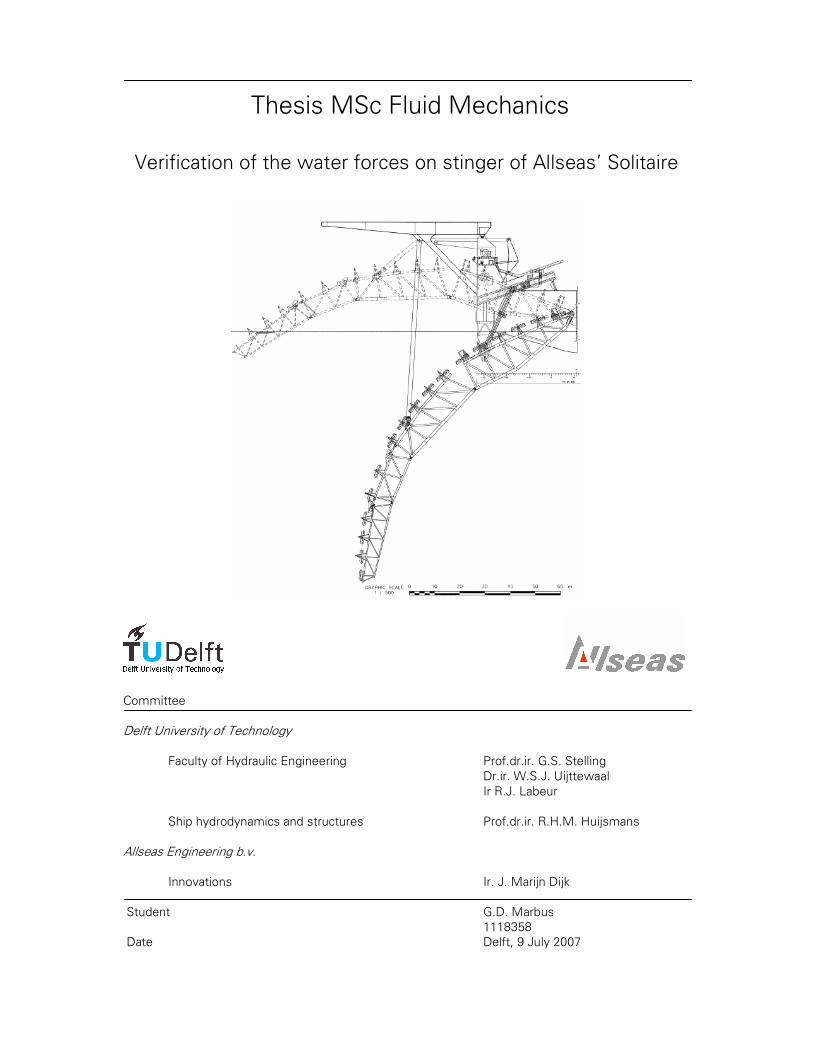
Verification of the water forces on stinger of Allseas’ Solitaire
Committee
Delft University of Technology Faculty of Hydraulic Engineering Prof.dr.ir. G.S. Stelling
Dr.ir. W.S.J. Uijttewaal
Ir R.J. Labeur
Ship hydrodynamics and structures Prof.dr.ir. R.H.M. Huijsmans
Allseas Engineering b.v. Innovations Ir. J. Marijn Dijk
Student G.D. Marbus
1118358
Date Delft, 9 July 2007

Verification of water forces on stinger of Allseas’ Solitaire
ii
©Copyright Allseas
This document is the property of Allseas and may contain confidential information. It may not be used
for any purpose other than for which it is supplied. This document may not be wholly or partly
disclosed, copied, duplicated or in any way made use of without prior written approval of Allseas

Verification of water forces on stinger of Allseas’ Solitaire
iii
Nomenclature
Glossary of terms
AQWA Program that calculates the hydrodynamic forces on structures in water due
to relative water motions.
Buckling Failure mode of the pipeline characterised by a failure to react to the bending
moment generated by a compressive load.
Cantilever Steel bridgework on the stern of Solitaire, on which the sheaves for the
stinger cables are placed.
Departure point Point where the pipeline leaves the stinger
Firing Line Line of workstations that work on the pipeline.
J — Lay Method of pipeline installation where the firing line is vertically placed on the
pipelay barge and the pipeline leaves the pipelay barge under a nearly vertical
departure angle, assuming the shape of a J.
Overbend Curved section of pipeline on the stinger
RAO Response Amplitude Operator presents the ratio between input amplitude of
an incoming wave and output amplitude of the motion of a structure
Stinger Tubular steel support frame attached to the stern of a pipelay vessel to limit
the bending of the pipe as it enters the water.
S — Lay Method of pipeline installation where the firing line is horizontally placed on
the pipelay barge and the pipeline leaves the pipelay barge under a nearly
horizontal angle, assuming the shape of a S after being supported by the
stinger into a nearly vertical departure angle.
Uplift A movement of the stinger in upward direction around the main hinge due to
water forces on the stinger.
Verification of water forces on stinger of Allseas’ Solitaire
iv
List of Symbols
a Acceleration [m2/s]
A Surface [m2]
Ca Disturbance Force Coefficient [-]
CD Drag coefficient [-]
CL Lift coefficient [-]
CM Inertia coefficient [-]
CP Pressure coefficient [-]
CFrms Total in line force coefficient [-]
D Diameter Cylinder [m]
E Ellipticity [-]
fv Vortex shedding frequency [1/s]
F Morison Force [N/m]
FD Drag Force [N/m]
FI Inertia Force [N/m]
FL Lift Force [N/m]
Fpressure Pressure Force [N/m]
Fr Froude number [-]
g Gravity acceleration [m/s2]
H Wave height [m]
Hu Response function [-]
KC Keulegan-Carpenter Number [-]
k Surface roughness [m]
k Wave number [1/m]
L Length [m]
N Number of samples [-]
p Pressure [kg/ms2]
p0 Undisturbed Pressure [kg/ms2]
Re Reynolds Number [-]
S Distance between tandem cylinders [m]
S Distance between staggered cylinders [m]
St Strouhal Number [-]
t Time [s]
T Period [s]
T Distance between side by side cylinders [m]
Ti Magnitude of Turbulence [-]
Tw Period of oscillatory flow [s]
ua Amplitude of a signal [ * ]
U Water velocity [m/s]
Um Maximum horizontal water velocity [m/s]
UN Flow velocity perpendicular on the cylinder [m/s]
U0 Undisturbed flow velocity [m/s]
Vm Maximum vertical water velocity [m/s]
Vol Volume [m3]
α Angle of flow with pair of cylinders [°]
αL Scale factor length [-]
αT Scale factor time [-]
αV Scale factor velocity [-]
αFI Scale factor inertia force [-]
αFG Scale factor gravity force [-]
αg Scale factor gravity [-]
αM Scale factor mass [-]
αρ Scale factor density [-]
αν Scale factor viscosity [-]
β Sarpkaya frequency parameter [-]
εFt Phase shift [rad]
Verification of water forces on stinger of Allseas’ Solitaire
v
ζ Wave elevation [m]
ζa Wave amplitude [m]
θ Angle of attack [°]
ρ Density of sea water [kg/m3]
ν Kinematic viscosity [m2/s]
ω Wave frequency [rad/s]
• Depends on used signal
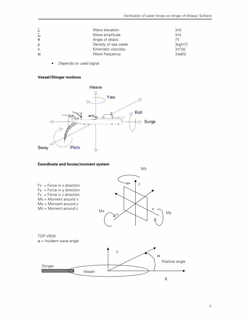
Vessel/Stinger motions
Coordinate and forces/moment system
Fx = Force in x direction
Fy = Force in y direction
Fx = Force in z direction
Mx = Moment around x
My = Moment around y
Mz = Moment around z
TOP VIEW
α = Incident wave angle
x
z
y Mx My
Mz
x
α Positive angle
y
Stinger
Vessel

Verification of water forces on stinger of Allseas’ Solitaire
vi
Verification of water forces on stinger of Allseas’ Solitaire
vii
Preface
This report contains the results of my thesis project. The thesis forms the final phase of the 2-year
MSc Hydraulic Engineering curriculum at the Delft University of Technology. The thesis work has
been performed at the Innovations department of Allseas Engineering BV in Delft where I started in
December 2006. The subject of the research project is the verification of the AQWA program, which
calculates the hydrodynamic forces on a pipelaying vessel.
I would like to thank my colleagues from Allseas Engineering for the co-operation during the project
and Marijn Dijk in particular. From the Msc Hydraulic Engineering I would like to thank Mr. Stelling, Mr
Uijttewaal and Mr. Labeur for their help. From the Faculty Ship Hydrodynamics and Structures I would
like to thank Mr. Huijsmans for his guidance, which greatly contributed. Finally, it is my parents that
made all this possible, I hope they know, how much the last 25 years meant to me.
Gerbrand Marbus
Delft, 9 July 2007

Verification of water forces on stinger of Allseas’ Solitaire
viii
Verification of water forces on stinger of Allseas’ Solitaire
ix
Summary
Allseas Engineering bv (“Allseas”) is a major offshore contractor, supplying the oil and gas industry
with their expertise in the field of marine pipeline installation. The Allseas’Solitaire is the largest
pipelaying vessel in the world and has been developed for installation of large diameter pipelines. The
pipelines are welded on the ship in a horizontal working plane causing the pipes to leave the vessel
horizontally. To prevent the pipe from bending or breaking due to its weight the pipe is guided by an
outrigger called the “stinger”. The stinger is constructed out of cylindrical elements and will convey
the pipeline into the water on its route to the seabed in a controlled curve.
To calculate the hydrodynamic forces on the stinger the program AQWA is used by Allseas. This
program calculates the Morison force for each element of the stinger separately. AQWA makes
simplifications in its calculation method and the drag and inertia coefficients in the Morison force
formula have to be estimated. The simplifications used by AQWA in the calculation of the forces on
the stinger could result in results that are not in line with reality.
In this thesis a verification of the AQWA program is made, which results in more knowledge on the
accuracy of the program. To obtain the objective of this thesis the following three main steps are
taken: determinations of the forces and flow phenomena on cylinder, an investigation of effects
neglected by AQWA and a comparison of AQWA with a model test. First the flow phenomena on
cylinder are treated, which results in the Morison force formula. This formula consists out of a drag
and inertia term. The force coefficients of the drag and inertia term are mainly determined by two
parameters: the Reynolds number (Re) and the Keulegan Carpenter number (KC). Secondly, AQWA
neglects several effects, which can change the stinger loads drastically. After all, in order to
determine the accuracy of the program, AQWA is compared with scale model tests done in 1993 and
2000 by Martime Research Institute Netherlands (“MARIN”).
AQWA has the facilities to determine the motions and loads of fully coupled bodies of mixed type, so
both diffracting bodies (vessel) and Morison bodies (stinger). The stinger is built out of tube elements
and the load on these tubes is calculated by means of the Morison force. AQWA calculates for each
time step the force for every element separately, ignoring the influence on each other. Adding all
these forces together results in a total force and moment on the articulation point stinger-vessel.
Allseas works in AQWA with a drag coefficient of 1.2 and an inertia coefficient of 2.0. This selection
of force coefficients is based on experiments executed in simple flow ignoring several effects.
However, a few of these effects can have a severe impact on the magnitude of the force coefficients.
From this investigation followed that only the effects of free stream turbulence, angle of attack,
interference and vortex shedding can cause a significant difference between AQWA and reality. Free
stream turbulence will cause a higher drag and inertia for Reynolds numbers after the drag crisis and a
lower before the drag crisis. The angle of attack problem is omitted by AQWA with the independence
principle. With this principle the velocity component perpendicular to the tube axis and the “normal”
drag coefficient is used in the Morison formula. Experiments show however, that this drag coefficient
increases with an increasing angle of attack. Interference in the stinger is a very complex problem.
The stinger was simplified to a construction of 4 major cylindrical elements to give an estimation of
the magnitude of interference in the stinger. Experiments show that the drag coefficient of the
shielded cylinder can significantly reduce. Also, vortex shedding is a phenomenon that is not taken
into account by AQWA. This phenomenon can cause lift forces perpendicular to the fluid velocity
direction.
In 1993 and 2000 Maritime Research Institute Netherlands (“MARIN”) executed scale model test on
the Solitaire and his stinger. The test was scaled with Froude scaling, which results in the same
Keulegan Carpenter number in the scale model test as in reality. However, due to this Froude scaling
the Reynolds number is 275 times smaller in the scale model test than in reality. The Reynolds
number is one of the main parameters that determine the drag and inertia coefficient in the Morison
equation. For a fair comparison between AQWA and the scale test, these scale effects had to be
taken into account and the adjusted drag and inertia coefficients had to be determined. The
information on the force coefficient is very limited for the combination of Reynolds and Keulegan
Verification of water forces on stinger of Allseas’ Solitaire
x
Carpenter numbers, at which the scale model tests were executed. Therefore, these force
coefficients had to be estimated on the basis of an extrapolation of Sarpkaya’s experiments and an
experiment executed by Kuhtz in the Reynolds and Keulegan Carpenter numbers range of the scale
model test. In both approaches there is a lot of uncertainty, which resulted in taking a range of force
coefficients of 1.9 —2.1 for the drag coefficient and 1.1 — 1.7 for the inertia coefficient.
In AQWA the same model was constructed as in the MARIN tests. To obtain a fair comparison
between the AQWA and MARIN stinger load results, the ship motions have to be the same in AQWA
as observed in the MARIN test. The ship motions of AQWA had to be calibrated by means of
changing the damping in the system. In AQWA, the ability to change the motions is limited, so not in
every case a satisfactory result could be obtained. For the irregular wave tests it was impossible to
obtain the same ship motions found in the MARIN scale tests. Despite these limitations, most of the
regular wave tests were calibrated to the same ship motions as in the MARIN scale tests.
The differences in stinger forces and moments between AQWA and MARIN were of limited
significance. Where the ship motions coincide, the loads on the stinger are in the same range and the
differences in the calculated loads were smaller then 15%. The current comparison of results shows
that AQWA underestimates the force in the z-direction and the moment around the y-axis, whilst the
other loads are overestimated. In the current tests the Morison force only consisted out of the drag
term. This trend can also be found back in the regular wave test, where the comparison shows an
underestimation by AQWA of the forces in x — and z — direction and the moment around the y —axis.
From the comparison it can also be seen that the ship motions have a great influence on the stinger
forces and moments. This effect can be assigned to the velocity square in the Morison equation,
which will have more influence than a decrease or increase of the drag coefficient.
The investigation of neglected effects showed that these effects could have a severe influence on
the accuracy of the AQWA results. However, the comparison versus MARIN showed that AQWA is
able to produce stinger load results within an error margin of 15%. Scale effects are an uncertain
factor in the comparison with a scale model test. This comparison also shows that the ship motions
have more significant influence on the stinger loads then the drag coefficient.
Verification of water forces on stinger of Allseas’ Solitaire
xi
TABLE OF CONTENTS
NOMENCLATURE............................................................................................................................................ III
PREFACE...........................................................................................................................................................VII
SUMMARY ......................................................................................................................................................... IX
TABLE OF CONTENTS.................................................................................................................................... XI
1 INTRODUCTION......................................................................................................................................... 1
1.1 INTRODUCTION ........................................................................................................................................ 1
1.2 PIPE LAYING METHODS ............................................................................................................................ 1
1.3 SOLITAIRE................................................................................................................................................ 2
1.4 STINGER................................................................................................................................................... 3
1.5 SCOPE OF WORK ....................................................................................................................................... 4
2 FLOW PHENOMENA AND FORCES ON A CYLINDER ..................................................................... 7
2.1 INTRODUCTION ........................................................................................................................................ 7
2.2 POTENTIAL FLOW .................................................................................................................................... 7
2.3 VISCOUS FLUID........................................................................................................................................ 8
2.4 IN LINE FORCES ........................................................................................................................................ 9
2.5 TRANSVERSE FORCE ...............................................................................................................................11
2.6 MOBILE POINT OF SEPARATION ...............................................................................................................12
3 AQWA APPROACH ...................................................................................................................................15
3.1 INTRODUCTION .......................................................................................................................................15
3.2 METHODOLOGY ......................................................................................................................................15
3.3 AQWA NAUT .......................................................................................................................................15
3.4 SELECTION OF MORISON DRAG AND INERTIA COEFFICIENT.....................................................................17
4 A CRITICAL ASSESSMENT OF AQWA ................................................................................................19
4.1 INTRODUCTION .......................................................................................................................................19
4.2 ENVIRONMENTAL CONDITIONS ...............................................................................................................19
4.3 DRAG AND INERTIA COEFFICIENT BASIC .................................................................................................20
4.4 INFLUENCE OF EFFECTS ON FORCE COEFFICIENTS....................................................................................25
4.5 INTERFERENCE OF TWO CYLINDERS ........................................................................................................34
4.6 VORTEX SHEDDING .................................................................................................................................43
4.7 FINAL DIFFERENCES ................................................................................................................................45
5 MARIN TESTS ............................................................................................................................................47
5.1 INTRODUCTION .......................................................................................................................................47
5.2 RESPONSE AMPLITUDE OPERATOR .........................................................................................................47
5.3 TEST 1: REPORT NO. 2.11861-1-GT/DT 1993 ........................................................................................47
5.4 TEST 2: REPORT NO. 15946-1-GT 2000..................................................................................................48
5.5 DATA ANALYSIS .....................................................................................................................................50
5.6 SCALE EFFECTS .......................................................................................................................................52
5.7 MEASUREMENT ERRORS..........................................................................................................................57
6 AQWA VERSUS MARIN ...........................................................................................................................59
6.1 INTRODUCTION .......................................................................................................................................59
6.2 AQWA MODEL ......................................................................................................................................59
6.3 SHIP MOTIONS .........................................................................................................................................59
6.4 MARIN TESTS 1993 VERSUS AQWA .....................................................................................................59
6.5 MARIN TESTS 2000 VERSUS AQWA .....................................................................................................67
6.6 INFLUENCE OF FORCE COEFFICIENTS .......................................................................................................70
6.7 CONCLUSION...........................................................................................................................................71
7 CONCLUSIONS AND RECOMMENDATIONS .....................................................................................73

Verification of water forces on stinger of Allseas’ Solitaire
xii
7.1 INTRODUCTION .......................................................................................................................................73
7.2 CONCLUSION ON NEGLECTED EFFECTS OF AQWA..................................................................................73
7.3 CONCLUSIONS ON COMPARISON AQWA VERSUS MARIN......................................................................73
7.4 RECOMMENDATIONS...............................................................................................................................74
REFERENCES.....................................................................................................................................................75
APPENDIX A: PERSONAL DATA...................................................................................................................77
APPENDIX B: STINGER SOLITAIRE ............................................................................................................79
APPENDIX C: AQWA INFORMATION .........................................................................................................83
APPENDIX D: STINGER DIMENSION AND INTERFERENCE DISTANCES.........................................85
APPENDIX E: MARIN SCALE MODEL DIMENSIONS TEST 1993 ..........................................................89
APPENDIX F: FROUDE SCALING .................................................................................................................91
APPENDIX G: MARIN SCALE MODEL DIMENSIONS TEST 2000..........................................................93
APPENDIX H: RESPONSE FUNCTION TRANSFORMATION..................................................................95
APPENDIX I: AQWA MODEL .........................................................................................................................97
APPENDIX J: RAO SHIP MOTIONS TEST 1993 ........................................................................................101
APPENDIX K: RAO SHIP MOTIONS MARIN TEST 2000 ........................................................................107
APPENDIX L: TEST SET UP..........................................................................................................................111

Verification of water forces on stinger of Allseas’ Solitaire
1
1 Introduction
1.1 Introduction
This first chapter forms an introduction of this master thesis. It will give some general and background
information about the pipe laying process and its different methods. The biggest ship of Allseas, the
Solitaire, is introduced and the stinger will be described.
1.2 Pipe laying methods
Allseas is an offshore contractor involved in pipeline installation projects. These pipelines are used for
transporting oil and gas from an offshore location to the shore. The oil or gas from the offshore
location will be pumped from a platform through pipelines (export lines) to a larger line (trunkline) to
which other platforms will also feed their oil and gas. The trunkline connects several platforms to
shore. Because of these different pipelines the diameter varies from 6” to 12” for the infield lines,
10” to 24“ for the export lines and 24” to 42” for the trunklines. The largest pipeline that is now
completed is the Ormen Lange transport pipeline with a length of about 1200 kilometer. There are
currently four methods for pipe laying methods; Towing, Reeling, J — Lay and S — Lay.
With the towing method the pipeline is constructed on the shore and after completion towed to the
planned destination and placed on the seabed. This method is mostly used to install bundles of
pipelines or other configurations that will not pass a stinger. The towing method is the least common
method, which is only suitable for short lengths and large diameters.
With the reeling method the pipes are welded onshore and then the pipeline is reeled onto a big reel
on a vessel. The vessel will go to the desired location and the pipeline will be unreeled and placed on
the seabed. Disadvantage is that the vessel has to return to the shore when its reel is emptied. The
reeling method is suited for small diameters pipe only, but can be used in a very large range of
depths. The advantage is that it is a fast installation method with very limited welding operation
onboard.
With the J — Lay method the pipeline is constructed entirely offshore. The pipeline section are welded
together vertically on board. A J — Lay vessel has a tower in which the pipeline sections are lined up
for welding. After a connection is made the vessel will move forward while the pipeline will move
downward, making room for the next pipeline section.
With the S —Lay method the pipeline sections are welded together in a horizontal-working plane. The
pipeline leaves the ship horizontally after a forward movement of the vessel. To bend the pipe to the
seafloor without risking the integrity of the pipe, a stinger is needed to guide the pipe in the bend
downwards (the ‘overbend’). An overall view of the S —Lay and the J —Lay method is shown in Figure
1-1.

Verification of water forces on stinger of Allseas’ Solitaire
2
Figure 1-1: J- lay and S-Lay method [1]
Both the J-Lay and the S-Lay method have their advantages and disadvantages. For the J —Lay it is a
problem that all the welding and coating has to take place on one level onboard, which will increase
construction time. However, because the pipe is inserted into the water vertically (‘no overbend’), the
bending forces and stresses on the pipe are relative low. The S — lay method is a faster installation
method for a large range of pipe diameters since work on the pipe can take place in multiple
workstations. It can lay pipes in a large range of depths due to the horizontal departing angle and the
adaptability of the stinger. For deep water the stresses and forces on the pipe in the ‘overbend’
become very large, which requires a very long stinger to reduce the stresses. Allseas only works with
the S-lay method. [1]
1.3 Solitaire
Founded in 1985, Allseas built its first vessel, Lorelay in 1985/1986. It is still one of the most modern
pipelay vessels in the world. One of her main characteristics is the Dynamic Positioning; this means
that the vessel is positioned by thrusters located at the front and rear of the vessel and not by
anchors.
The Trenchsetter was built in 1989 as a support for other vessels, but in 2005 Calamity Jane replaced
the Trenchsetter. In 1996 the Tog Mor was bought for constructing pipelines in shallow water. In
1988, Solitaire was the second Allseas S- Lay pipe-laying vessel in operation, the third vessel,
Audacia, is currently under construction and will be finished in July 2007.
The Solitaire was built on the same base as the Lorelay. The advantages of the horizontal working
plane and the DP system created a fast installation method for installing pipelines. The Solitaire is the
largest pipelay vessel in the world with a pipe carrying capacity of 22.000 tonnes. Due to the DP
system the Solitaire can work in busy areas, whilst a high cruising speed and lay rate makes her
competitive worldwide. An overview of the vessel is given in Figure 1-2.
Verification of water forces on stinger of Allseas’ Solitaire
3
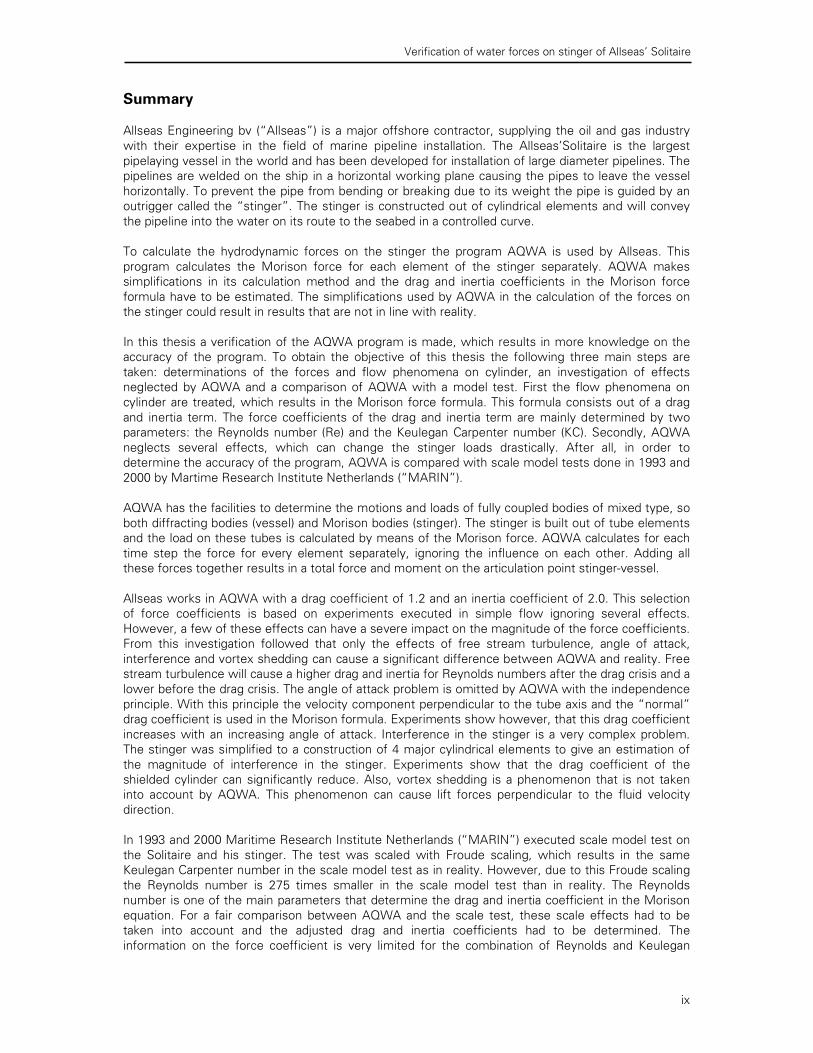
Figure 1-2: Solitaire [1]
Solitaire has been developed for the installation of large pipes, with a maximum diameter of 60”, at
laying speeds of about 4 tot 7 kilometer per day. The workability of the Solitaire is better than the
Lorelay and it is able to work in wave heights up to about 4 meters, which means that it can work
almost throughout the year. [2]
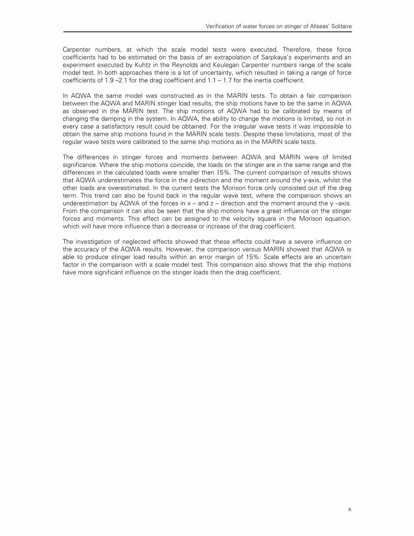
1.4 Stinger
The S — Lay method, with its horizontal working plane, causes the welded pipelines to leave the
vessel horizontally. When looking at Figure 1-1, It is obvious that the pipes weight will cause a force
downward on the horizontal section that is leaving the ship. When nothing is done the pipeline can
break or bend heavily, which is called ‘buckling’. This is why the pipe is fed on to an outrigger called
the “stinger”, in a gentle bend (“overbend”), see Figures 1-2 and 1-3. The stinger will convey the
pipeline into the water on its route to the seabed in a controlled curve.
1
2
3
4
Figure 1-3: Overview stinger with the 4 sections in two different positions [1]
Verification of water forces on stinger of Allseas’ Solitaire
4
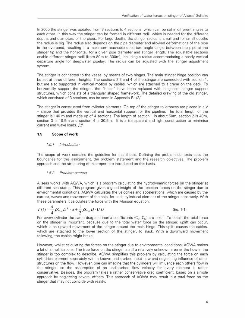
In 2005 the stinger was updated from 3 sections to 4 sections, which can be set in different angles to
each other. In this way the stinger can be formed in different radii, which is needed for the different
depths and diameters of the pipes. For large depths the stinger radius is small and for small depths
the radius is big. The radius also depends on the pipe diameter and allowed deformations of the pipe
in the overbend, resulting in a maximum reachable departure angle (angle between the pipe at the
stinger tip and the horizontal) for a given pipe diameter and stinger length. The adjustable sections
enable different stinger radii (from 80m to 300m), including a radius accommodating a nearly vertical
departure angle for deepwater pipelay. The radius can be adjusted with the stinger adjustment
system.
The stinger is connected to the vessel by means of two hinges. The main stinger hinge position can
be set at three different heights. The sections 2,3 and 4 of the stinger are connected with section 1,
but are also supported in vertical motion by cables, which are attached to a crane on the deck. To
horizontally support the stinger, the “heels” have been replaced with hingeable stinger support
structures, which consists of a triangular shaped framework. The detailed drawing of the old stinger,
which consisted of 3 sections, can be seen in Appendix B. [2]
The stinger is constructed from cylinder elements. On top of the stinger rollerboxes are placed in a V
— shape that provides the vertical and horizontal support for the pipeline. The total length of the
stinger is 140 m and made up of 4 sections. The length of section 1 is about 50m, section 2 is 40m,
section 3 is 19,5m and section 4 is 30,5m. It is a transparent and light construction to minimise
current and wave loads. [3]
1.5 Scope of work
1.5.1 Introduction
The scope of work contains the guideline for this thesis. Defining the problem contexts sets the
boundaries for this assignment, the problem statement and the research objectives. The problem
approach and the structuring of this report are introduced on this basis.
1.5.2 Problem context
Allseas works with AQWA, which is a program calculating the hydrodynamic forces on the stinger at
different sea states. This program gives a good insight of the reaction forces on the stinger due to
environmental conditions. AQWA calculates the velocities and accelerations, which are caused by the
current, waves and movement of the ship, for each cylindrical element of the stinger separately. With
these parameters it calculates the force with the Morison equation:
UUDCaDCtF Dm ⋅+⋅= ρρπ
2
1
4)(
2 (Eq. 1-1)
For every cylinder the same drag and inertia coefficients (CD, CM) are taken. To obtain the total force
on the stinger is important, because due to the total water force on the stinger, uplift can occur,
which is an upward movement of the stinger around the main hinge. This uplift causes the cables,
which are attached to the lower section of the stinger, to slack. With a downward movement
following, the cables might brake.
However, whilst calculating the forces on the stinger due to environmental conditions, AQWA makes
a lot of simplifications. The true force on the stinger is still a relatively unknown area as the flow in the
stinger is too complex to describe. AQWA simplifies this problem by calculating the force on each
cylindrical element separately with a known undisturbed input flow and neglecting influence of other
structures on the flow. However, one can imagine that the cylinders will influence each others flow in
the stinger, so the assumption of an undisturbed flow velocity for every element is rather
conservative. Besides, the program takes a rather conservative drag coefficient, based on a simple
approach by neglecting several effects. This approach of AQWA may result in a total force on the
stinger that may not coincide with reality.

Verification of water forces on stinger of Allseas’ Solitaire
5
This approach of AQWA is valid, but rather conservative. This is not a bad approach, but due to this
conservative way of working, the actual flows and forces are not known. Allseas wants to know how
accurate the program AQWA calculates the hydrodynamic forces and what simplifications it makes.
1.5.3 Problem Statement
Allseas calculates the water forces on the stinger with AQWA and wants to assess the accuracy of
this program. Also, more knowledge is needed on the simplifications AQWA. A study is needed to
verify this program.
1.5.4 Research Objective
The objective of this thesis is to verify the water forces on the stinger calculated by AQWA, which
results in more knowledge on the accuracy of this program.
1.5.5 Problem approach
To obtain the objective of this thesis the following three main steps are proposed; determination of
the forces and flow phenomena on cylinders, investigating of the neglected effects in the program
and a comparison of AQWA with a model test.
In chapter 2 the forces on simple single vertical circular cylinder are described. All the phenomena,
which occur on a cylinder, are determined and a view on forces on cylinders is obtained. Furthermore;
previous experiments are discussed in order to get more knowledge about the force coefficients at
different states.
A close investigation will take place on the working of AQWA to get a better understanding of this
program in chapter 3. The approach used in the AQWA calculations is investigated.
In chapter 4 a critical assessment is done for the program AQWA. All the effects that are neglected
by the program are determined to get insight in the accuracy of the AQWA program. First the
environmental conditions are described for which the force coefficients are determined. These
environmental conditions are based on classification notes from Det Norske Veritas. Then several
effects and their influence on the force coefficients are investigated, based on previous experiments.
These results will be applied on the cylinders to explain the difference between AQWA and the tests.
The impact of the different effects is also investigated, which tries to explain the great difference
between AQWA and the tests.
In 1993 and 2000 scale tests were done with the Solitaire and its old stinger in the MARIN laboratory.
Forces are measured on the stinger. These forces are scaled and a comparable data is obtained.
These tests are used to verify the AQWA working method. This process is addressed in chapter 5.
The scaling of the flow conditions is also discussed in this chapter.
In chapter 6 the MARIN test data is available to compare with the program AQWA. For the
comparison of the MARIN test, the same water conditions used in this test are put in AQWA on the
same stinger. A difference in forces is obtained and the cause of these differences is investigated.
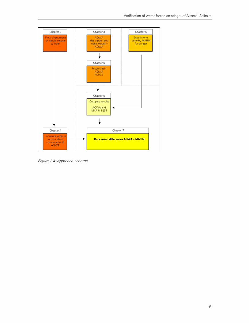
In Chapter 7 the final conclusions and recommendations for further studies are given. In Figure 1-4
the approach scheme is given to finally come to these conclusions.
Verification of water forces on stinger of Allseas’ Solitaire
6
Chapter 2
Flow phenomenaon single vertical
cylinder
Chapter 5
Chapter 7
Chapter 6
Chapter 3
Chapter 6
Chapter 4
Influence effectson cylinders
compared withAQWA
Experimentsdone by MARINfor stinger
AQWAdescription andmake Model in
AQWA
Modelling inAQWAFORCE
Compare results
AQWA andMARIN TEST
Conclusion differences AQWA v MARIN
Figure 1-4: Approach scheme

Verification of water forces on stinger of Allseas’ Solitaire
7
2 Flow phenomena and forces on a cylinder
2.1 Introduction
The stinger is built out of cylindrical pipes. To calculate the forces on the structure, a view on the
theory of forces on a cylinder due to wave forces and currents, has to be obtained. This is done in this
chapter with the assumption that all cylinders are slender cylinders. This implies that its diameter is
relatively small to the wavelength. The formulas and other derivations are done for a unit length of
cylinder.
2.2 Potential Flow
A steady flow of an incompressible (potential) fluid yields a relationship called the Bernoulli equation.
It is a relationship between the change in kinetic energy and the work done on a water particle.
=+g
U
gh
p
2
2
ρ Constant (Eq. 2-1)
This formula states that the sum of the piezometric and kinetic pressure is constant along a
streamline for the steady flow of an incompressible, non-viscous fluid. It is often convenient to
express the pressure in terms of a non-dimensional quantity called the pressure coefficient, which is
defined as
2
0
0
5.0 U
ppC p
ρ
−= (Eq. 2-2)
A negative pressure coefficient means that the local pressure is less than the reference pressure. If a
non-viscous and incompressible fluid is considered, then the Bernoulli equation will apply everywhere
in the flow field. The flow pattern on a circular cylinder is shown in Figure 2-1.
Figure 2-1: Potential flow around circular cylinder [4]
Point B is considered as 0° and point D as 180°. It is seen that the flow is symmetrical through the
centre of the cylinder in vertical and horizontal sense. This is also applied to the pressure distribution
along the cylinder surface, which is illustrated in Figure 2-2.
Figure 2-2: Pressure distribution around cylinder for potential flow [4]
B

Verification of water forces on stinger of Allseas’ Solitaire
8
Figure 2-2 shows that the pressure at 0° and 180° is the same for an ideal fluid, so there will be no
total pressure gradient on the cylinder. However, a water particle travelling from 0° to 180° along the cylinder surface will be exposed to different conditions. Before it hits the cylinder it decelerates,
which is consistent with a high pressure at the stagnation point 0°. Then it accelerates from 0° to 90° to its maximum speed by the action of the pressure gradient and the pressure will decrease along
this path to the midsection. As the particle travels from 90° to 180°, its momentum is sufficient to
allow it to travel further against the adverse pressure gradient. [4]
2.3 Viscous Fluid
Previously ideal non-viscous fluid was treated. However, in reality fluid has a viscous character. This
will have a significant influence on the flow pattern around a cylinder. The viscous character of the
fluid causes that the velocity at the surface of the cylinder is zero. Because of this viscous effect a
thin layer is produced, which is called a boundary layer. The velocity in this layer changes from zero to
the free stream velocity and the flow in this layer can be either laminar or turbulent (Figure 2-3).
Figure 2-3: Boundary layer [4]
Different definitions are available for the description of a flow around a cylinder. These flows are
determined by the characteristics of the free stream velocity, cylinder diameter and fluid dynamic
viscosity, which are all combined in a non dimensional number called the Reynolds number:
ν
DU ⋅=Re (Eq. 2-3)
In case the cylinder is exposed to an oscillatory flow an additional parameter — the Keulegan-
Carpenter number — is used. This number is defined by
D
TUKC wm ⋅
= (Eq. 2-4)
Besides this, the roughness of the surface and the turbulence in the free stream flow affects the flow
pattern around the cylinder. The different states of flow around a cylinder are shown in Figure 2-4 and
described from low velocity to high velocity. The characteristics of the different states are described
in Table 2-1.
Figure 2-4: Flow regimes [5]

Verification of water forces on stinger of Allseas’ Solitaire
9
Flow definition Character
Laminar Laminar vortex street
Transition wake Transition to turbulence wake
Subcritical Wake completely turbulent
Laminar boundary layer separation
Critical lower transition Laminar boundary layer separation
Start of turbulent boundary layer separation
Supercritical Turbulent boundary layer separation; the boundary
layer partly laminar partly turbulent
Uppertransition Boundary layer completely turbulent at one side
Transcritical Boundary layer completely turbulent at two sides
Table 2-1: Regimes of flow around a circular cylinder [5]
2.4 In line forces
2.4.1 Drag forces
Downstream of the midsection (90°-180°), the pressure increases with distance along the surface.
The velocity decreases along the surface in the boundary layer, while the pressure is increasing in
adverse direction. At a certain moment the pressure gradient forces the fluid to detour away from the
surface, which is called the separation point. The circular flow behind the cylinder is called the wake
(Figure 2-5).
Figure 2-5: Viscous flow around cylinder with wake [4]
The Re number, KC number and several other considerations determine the point of separation. In
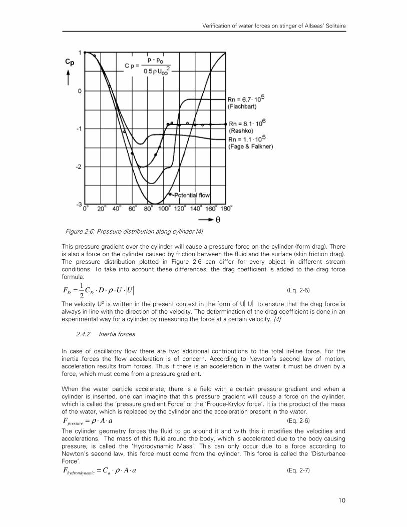
Figure 2-6 the pressure distribution over the cylinder is shown and a difference in upstream and
downstream pressure is seen for a viscous fluid in comparison with the similarity of the potential
flow. The pressure at 0° is not the same as at 180°, which is caused by the separation and the
occurrence of the wake.
Verification of water forces on stinger of Allseas’ Solitaire
10
Figure 2-6: Pressure distribution along cylinder [4]
This pressure gradient over the cylinder will cause a pressure force on the cylinder (form drag). There
is also a force on the cylinder caused by friction between the fluid and the surface (skin friction drag).
The pressure distribution plotted in Figure 2-6 can differ for every object in different stream
conditions. To take into account these differences, the drag coefficient is added to the drag force
formula:
UUDCF DD ⋅⋅⋅⋅= ρ2
1 (Eq. 2-5)
The velocity U2 is written in the present context in the form of UU to ensure that the drag force is always in line with the direction of the velocity. The determination of the drag coefficient is done in an
experimental way for a cylinder by measuring the force at a certain velocity. [4]
2.4.2 Inertia forces
In case of oscillatory flow there are two additional contributions to the total in-line force. For the
inertia forces the flow acceleration is of concern. According to Newton’s second law of motion,
acceleration results from forces. Thus if there is an acceleration in the water it must be driven by a
force, which must come from a pressure gradient.
When the water particle accelerate, there is a field with a certain pressure gradient and when a
cylinder is inserted, one can imagine that this pressure gradient will cause a force on the cylinder,
which is called the ‘pressure gradient Force’ or the ‘Froude-Krylov force’. It is the product of the mass
of the water, which is replaced by the cylinder and the acceleration present in the water.
aAFpressure ⋅⋅= ρ (Eq. 2-6)
The cylinder geometry forces the fluid to go around it and with this it modifies the velocities and
accelerations. The mass of this fluid around the body, which is accelerated due to the body causing
pressure, is called the ‘Hydrodynamic Mass’. This can only occur due to a force according to
Newton’s second law, this force must come from the cylinder. This force is called the ‘Disturbance
Force’.
aACF amichydrondyna ⋅⋅⋅= ρ (Eq. 2-7)

Verification of water forces on stinger of Allseas’ Solitaire
11
Both forces result in a total inertia force, which is formulated as:
aDCtF mI ⋅⋅= 2
4)(
πρ (Eq. 2-8)
With:
am CC += 1 (Eq. 2-9)
Cm is the experimental inertia coefficient, which consists of the coefficients of the two forces. For the
pressure gradient force the coefficient is always 1, but for the disturbance force the coefficient is not
a fixed value and differs for every stream condition and the characteristics of the element.
2.4.3 Morison Equation
Now the total in-line force can be formulated for an accelerated water environment where the cylinder
is held stationary. The total force, ( )tF , is give by equation 3-8 with, in sequence, the inertia force
and the drag force.
UUDCaDCtF Dm ⋅⋅⋅+⋅⋅⋅= ρρπ
2
1
4)(
2 (Eq. 2-10)
There will be a 90° phase difference between the maximum value of drag force and the maximum value of inertia force.
2.5 Transverse Force
As described earlier, the boundary layer over the cylinder surface will separate due to the adverse
pressure gradient imposed by flow environment at the downstream side. The boundary layer contains
a significant amount of vorticity. This vorticity is fed into the shear layer formed downstream of the
separation point and causes the shear layer to roll up into a vortex (Figure 2-7).
Figure 2-7: Boundary layer separation with vorticity [5]
Likewise, a vortex, rotating in the opposite direction, is formed at the other side of the cylinder. One
of the vortices becomes strong enough to draw the opposing vortex across the wake. The vorticity of
this approaching vortex will have a vorticity of the opposite sign and will then cut off further supply of
vorticity to the stronger vortex from its boundary layer. The upper vortex is shed what is shown in
Figure 2-8.
Figure 2-8: Vortex shedding [5]

Verification of water forces on stinger of Allseas’ Solitaire
12
This same process will now happen at the other side, because that is now the stronger vortex side.
This process will continue every time a new vortex is shed. The vortex shedding frequency can be
seen as a function of the Reynolds number and the surface roughness and is called the Strouhal
number [5]:
U
Df
D
kStSt v=
= Re, (Eq. 2-11)
A lift force is defined as a force component acting perpendicular to the undisturbed flow velocity. It is
therefore also perpendicular to the drag force component. In a potential flow there will be no lift
force, but as a consequence of the vortex-shedding phenomenon, the pressure distribution around
the cylinder undergoes a periodic change. At the location where the vortex is closest to the cylinder
the local velocities in the wake will be the highest and the local pressures will be lowest. This results
in a force directed toward the vortex:
)2sin(2
1 2
FtvLL tfCDUF επρ +⋅⋅⋅= (Eq. 2-12)
The lift force will alternate in direction, because of the vortices are shed alternately. The formula of
the lift force. When the vortex frequency coincide with the natural frequency of the cylinder, then big
vortex induced oscillations can happen. This is an unwanted occurrence for any a structure as it
induces heavy vibrations in the structure itself. [6]
2.6 Mobile point of separation
As mentioned before, the point of separation will depend on the characteristics of the flow. The
separation point is mobile on a circular cylinder, and its motion is coupled with the shedding of the
vortices. The vorticity feeding the shear layer fluctuates with time since the separation point moves
into higher and lower velocity regions. When the vortices, vortex feeding layers, and even the
boundary layer over the forebody become turbulent, significant changes take place in the forces
acting on the body.
An experimental study by Roshko and Fiszdon (1969) has shown that when the Reynolds number(Re)
is between 1 and 50, the entire flow is laminar and steady. When the Reynolds number increases to
50-200, the flow retains its laminar character, but the near wake becomes unstable. If Re is about
1500, turbulence will occur and spreads downstream. Further increasing of Re to 1500 — 2x10⁵
causes the transition to turbulence to move upstream along the free shear layer and the wake to
become irregular.
When the transition coincides with the separation point at a Re of about 5x10⁵, the flow first
undergoes a laminar separation, followed by a reattachment to the cylinder, and then a turbulent
separation to form a narrower wake. This results in a large fall in both the lift and the drag coefficient.
It leads to a sharp decrease of the drag force, which is known as the “drag crisis”. This transition in
drag coefficient is due to transition of the separated boundary layer to a turbulent state, the formation
of a separation bubble, reattachment of the rapidly spreading turbulent free shear layer, and finally,
separation of the turbulent boundary layer at a position further downstream from the first point of
laminar separation.
The reduction of the wake size as a consequence of the retreat of the separation point then results in
a smaller form drag. An of Re 106 to 107 can then be interpreted as a transition to a turbulent state of
the attached portion of the boundary layer. In Figure 2-9 the force coefficient is plotted against the
Reynolds number. While considering a steady flow, one must realise that there will be no inertia
force.

Verification of water forces on stinger of Allseas’ Solitaire
13
Figure 2-9: Global curve drag coefficient versus Re [5]
It is important to remember that the Reynolds numbers at which these phenomena occur depends
very much on the character of the flow. The above used Reynolds numbers were for a smooth and
steady flow. So the exact number will not be the same for a rough surface and a time-dependent
flow. However, the sequence of these phenomena will be the same, but only occur at different
Reynolds numbers. In general, it is worth remembering that the flow is sensitive to a lot of
parameters (roughness, free-stream turbulence, vibrations, end conditions etc.). [5]

Verification of water forces on stinger of Allseas’ Solitaire
14

Verification of water forces on stinger of Allseas’ Solitaire
15
3 AQWA approach
3.1 Introduction
Before verifying the AQWA program in comparison with the MARIN model test a good understanding
of AQWA has to be obtained. First the methodology of the program is described and the main
calculating program AQWA-NAUT is analysed in this chapter. In Appendix C a more detailed
description is given.
3.2 Methodology
The basis of the AQWA program is basic diffraction theory. The AQWA suite has the facilities to
determine the motions and loads of fully coupled bodies. These bodies may be of mixed type, so
diffracting bodies (vessel) and Morison bodies (stinger). The AQWA program suite consists of
different programs, of which full descriptions are given in Appendix C. For the vessel, use is made of
AQWA LINE, for further modelling AQWA LIBRIUM is used and for the stinger AQWA DRIFT and
AQWA NAUT are used, which is a time domain based program.
The first analysis is with AQWA LINE and is the determination of the diffraction characteristics of the
pipe- lay vessel “Solitaire” for several frequencies and directions. Then the stinger is attached to the
model and with the result of the AQWA LINE analysis the motions of the stinger - vessel combination
is calculated in AQWA LIBRIUM and an equilibrium position is found. The point where the vessel and
stinger are attached together is called “articulation point” .In this analysis the vessel and the stinger
are attached, so the influences of these two on each other are included in the calculations. The last
AQWA NAUT analysis is a time-domain simulation to determine the loads and motions on the stinger.
[7]
A diffraction model is made of the hull and a complete tubular structure is made for each stinger
section, which is modelled as one object. The stinger section models and the heel models are built up
by TUBE elements and slender (plate) elements, each with its specific dimensions and weight. An
example of a model in AQWA is given in Figure 3-1.
3.3 AQWA NAUT
This part of the AQWA program suite does the calculations of the forces on the stinger with the
Morison equation. This thesis is mainly about comparing the results of this program with the results
obtained by the MARIN model tests.
The location of any point in the structure in the modelling process is determined by referring to the
X,Y and Z co-ordinate of that point in the fixed reference axes, which is termed a NODE. The model of
structure geometry and mass distribution consists of a specification of one or more elements whose
position is that of a node. Nodes may be thought of as a table of numbers and associated co-ordinate
points, which other parts of the model refer to. The structural geometry and mass distribution of the
Figure 3-1: Models in AQWA

Verification of water forces on stinger of Allseas’ Solitaire
16
model for AWQA NAUT is achieved by specifying one or more elements, which in total describe the
whole structure.
Morison forces, which are applicable to small tubular structures or parts of structures, can be included
in an AQWA-NAUT analysis by the use of TUBE elements. The forces are calculated at each time
step. The force (normal to the tube axis) on a TUBE element is given by:
aClDF
alDF
lDUUCF
FFFF
aaWaveInerti
ovFroudeKryl
DDrag
aWaveInertiKrylovFroudeDragMorison
⋅⋅⋅⋅⋅=
⋅⋅⋅⋅=
⋅⋅⋅⋅⋅=
++= −
2
2
4
4
5.0
πρ
πρ
ρ
(Eq. 3-1)
The velocity and acceleration used in AQWA are the fluid velocity/acceleration minus the structure
velocity/acceleration. This way the relative velocity/acceleration is considered. In this approach the
influence from the ship’s hull on the fluid velocity/acceleration is ignored. Full account is taken of fluid
velocity variation over the length. AQWA calculates the relative velocity and acceleration at the two-
point Gauss positions (+/- 0.5773) based on the wetted length and then does a linear integration.
AQWA calculates the velocity and acceleration for each TUBE element separately and calculates from
these the Morison forces for every element. These forces are divided into forces in the x -, y- and z —
direction, which acts in the center of gravity of each TUBE element. These forces of all elements are
added together by AQWA what results in a total force in the articulation point of stinger — vessel in
three directions (Figure 3-2). The forces on each element can be recalculated to a moment around the
main hinge. This is also done for the three direction forces on each element times the perpendicular
distance to the articulation point. An overview of the forces and moments calculated in AQWA is
given in Figure 3-2.
Fx
Fz
Fy
My
Mx
Fy Fz
Fx
Mz
Figure 3-2: Force and moment direction in articulation point
Verification of water forces on stinger of Allseas’ Solitaire
17
With the known buoyancy and weight of the structure, it is possible to calculate what the moment
and force is in the main hinge at the ship. When the force of the environmental conditions is higher
than the forces of buoyancy and weight, uplift of the stinger will occur. [7]
3.4 Selection of Morison drag and inertia coefficient
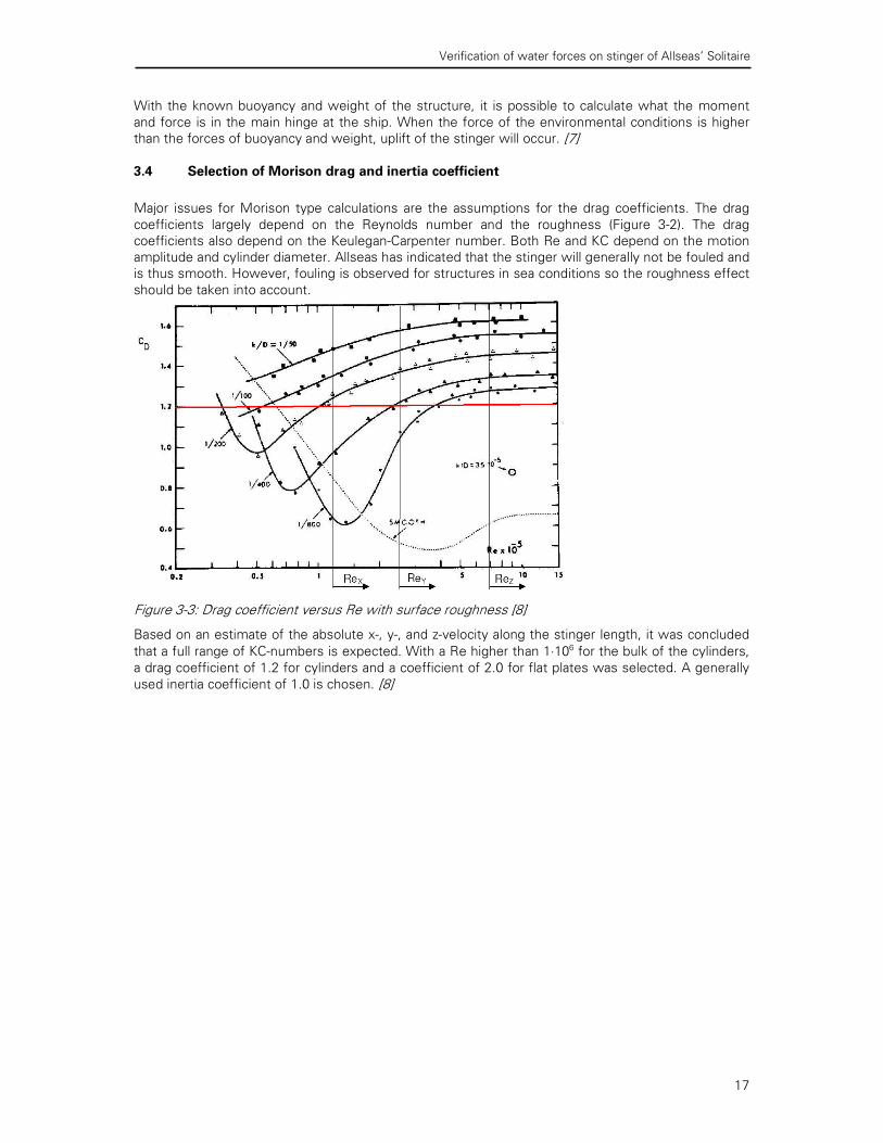
Major issues for Morison type calculations are the assumptions for the drag coefficients. The drag
coefficients largely depend on the Reynolds number and the roughness (Figure 3-2). The drag
coefficients also depend on the Keulegan-Carpenter number. Both Re and KC depend on the motion
amplitude and cylinder diameter. Allseas has indicated that the stinger will generally not be fouled and
is thus smooth. However, fouling is observed for structures in sea conditions so the roughness effect
should be taken into account.
Figure 3-3: Drag coefficient versus Re with surface roughness [8]
Based on an estimate of the absolute x-, y-, and z-velocity along the stinger length, it was concluded
that a full range of KC-numbers is expected. With a Re higher than 1⋅106 for the bulk of the cylinders,
a drag coefficient of 1.2 for cylinders and a coefficient of 2.0 for flat plates was selected. A generally
used inertia coefficient of 1.0 is chosen. [8]
Verification of water forces on stinger of Allseas’ Solitaire
18
Verification of water forces on stinger of Allseas’ Solitaire
19
4 A critical assessment of AQWA
4.1 Introduction
AQWA calculates the forces on the stinger with the Morison equation. The drag and inertia
coefficients, for this formula, are obtained from available information from experiments executed by
Sarpkaya. However, in reality the force coefficients in this formula will not only depend on the
Reynolds number, KC number, diameter and roughness as assumed in AQWA. The influences of
several other effects can cause drastic changes in the magnitude of these force coefficients. The
influences of waves, orbital motion, angle of attack, free stream turbulence, free ends and
interference on the force coefficients are investigated in this chapter. By not taking into account these
effects on the force coefficients, the assumed Cd = 1.2 and Cm = 2.0 as AQWA input may not be
correct. Furthermore AQWA does not take into account lift forces either. First the applicable
environmental conditions for the analysis of the stinger are determined.
4.2 Environmental conditions
Before determining the force coefficients and the neglected effects the range of Reynolds and
Keulegan Carpenter numbers must be determined for the cylindrical elements in the stinger. Looking
at the environmental conditions in which the Solitaire works will give these ranges of Re and KC
number.
Classification Notes are publications, which give practical information on classification of ships and
other objects. The DNV (Det Norske Veritas) has classification notes number 30.5, which are called
“Environmental conditions and environmental loads”, March 2000. These notes give guidance for
descriptions of important environmental conditions as well as environmental loads. Environmental
conditions cover natural phenomena, which may contribute to structural damages, operation
disturbances or navigation failures. These classification notes give parameters for the worldwide trade
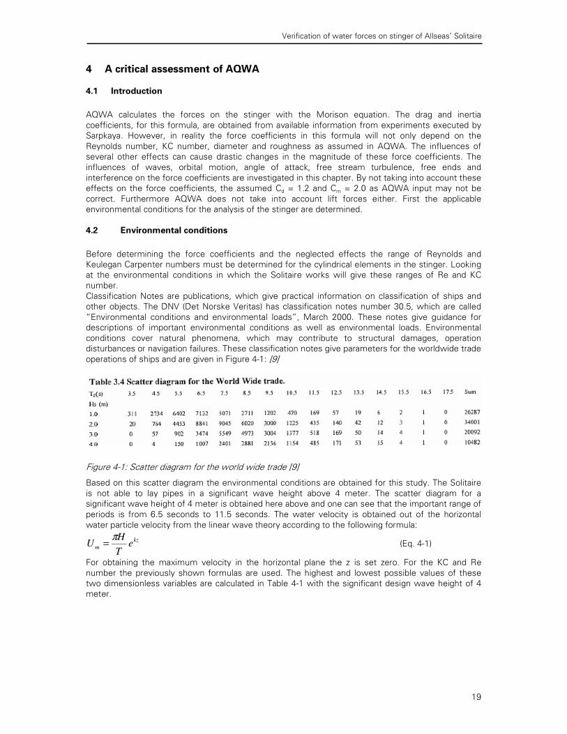
operations of ships and are given in Figure 4-1: [9]
Figure 4-1: Scatter diagram for the world wide trade [9]
Based on this scatter diagram the environmental conditions are obtained for this study. The Solitaire
is not able to lay pipes in a significant wave height above 4 meter. The scatter diagram for a
significant wave height of 4 meter is obtained here above and one can see that the important range of
periods is from 6.5 seconds to 11.5 seconds. The water velocity is obtained out of the horizontal
water particle velocity from the linear wave theory according to the following formula:
kz
m eT
HU
π= (Eq. 4-1)
For obtaining the maximum velocity in the horizontal plane the z is set zero. For the KC and Re
number the previously shown formulas are used. The highest and lowest possible values of these
two dimensionless variables are calculated in Table 4-1 with the significant design wave height of 4
meter.

Verification of water forces on stinger of Allseas’ Solitaire
20
Wave Height [m] 4
Periods T [s] 5.5 — 12.5
Velocity U [m/s] 1.1 — 1.9
Viscosity [m2/s] 1.36*10-6 (seawater 10°)
Diameter cylinder [m] 0.200 — 0.950
Re [-] 1.4*105 — 1.6*106
KC [-] 13 — 63
Table 4-1: Environmental conditions
The calculated ranges of Re and KC number is used for every graph of force from here on. The values
are very high and can be considered supercritical to transcritical.
4.3 Drag and Inertia coefficient basic
4.3.1 Harmonically flow smooth cylinder
In this paragraph attention is given to harmonically oscillating flow, which results in a time dependent
flow. When a cylinder is subjected to a harmonic flow normal to its axis, the flow does not only
accelerate and decelerate, but also changes direction during each cycle. The wake changes from side
to side and this produces large excursions of the separation points. Due to harmonic flow it is
possible to separate the additional effect of a wave climate from the periodic reversal of the flow in
waves.
Harmonic flow around cylinders has been investigated by a number of researchers. Because now
there is a time-dependent flow, the force coefficients are determined by the Reynolds number and
the Keulegan-Carpenter number. Also vortex-shedding regimes can be made, varying with the KC
number (Figure 4-2).
Figure 4-2: Flow regimes dependent of KC number
Experiments done by Sarpkaya (1976) [10] are taken as information source; he worked with a frequency parameter:
T
D
KC νβ
2Re
== (Eq. 4-2)
In his experiments he stated that the KC number, the frequency parameter and the surface
roughness determine the force coefficients. Notice that the Reynolds number is hidden in the
frequency parameter. β is constant for a series of experiments if the diameter and T are kept
constant. This way the variation of a force coefficient with KC may be plotted for constant values of β. In the case of the stinger, the range of the frequency parameter can be determined with the already
determined range of Re and KC. The frequency parameter will be in the range of

Verification of water forces on stinger of Allseas’ Solitaire
21
β = 57704 — 102092 for KC = 13
β = 2557 — 4524 for KC = 63
Sarpkaya (1976) conducted a series of experiments with smooth cylinders in a novel, U-shaped
vertical water tunnel. In these experiments the drag and inertia coefficients have been evaluated
through the use of Fourier analysis (Figure 4-3).
Figure 4-3: CD and CM versus KC for various values of frequency parameter tests by T. Sarpkaya (1976) [10]

Verification of water forces on stinger of Allseas’ Solitaire
22
This entire data are also shown as a function of Re for constant values of KC in Figure 4-4.
Figure 4-4: CD and CM versus Re for various values of KC tests by T. Sarpkaya (1976) [10]
Figures 4-3 and 4-4 clearly show that CD decreases with increasing Re to a value of about 0.6
(depending on KC) and then gradually rises to a constant value (post-supercritical value) within the
range of Reynolds numbers encountered. The inertia coefficient increases with increasing Re,
reaches a maximum, and then gradually approaches a value of about 1.85. The Figure 4-4 shows that
the drag coefficient in harmonically oscillating flow is not always larger than that for steady flow at the
same Reynolds number. The reason for this is the earlier transition in the boundary layer from laminar
to turbulent. The key to the understanding of the instantaneous behaviour of drag, lift and inertia
forces is the understanding of the formation, growth and motion of the vortices. For the stinger the
force coefficients stated in Table 4-2 holds.

Verification of water forces on stinger of Allseas’ Solitaire
23
Coefficient Minimum Maximum
Drag CD 0.51 0.7
Inertia CM 1.55 1.85
Table 4-2: Drag and inertia coefficients for harmonically oscillating flow
4.3.2 Roughness effects on force coefficients
Roughness is expressed as the ratio of the mean height of the roughness elements, k, to the
diameter of the cylinder, D. If the height of the roughness elements does not affect the flow around
a cylinder, the cylinder can be considered smooth. Prandtl did another approach for smooth surfaces:
“Slightly rough surfaces may be regarded smooth when the irregularities are completely embedded in
the laminar boundary layer. At high Re, when the laminar boundary layer becomes thinner, such
roughness may become effective causing an increase in drag. The approach used by Karman said: “
All surfaces may be considered rough when Re is sufficiently high because the frictional resistance of
the rough surface is made up essentially of the resistances of all the rough elements k, and those
become independent of the skin friction at high values of Re”
The turbulent boundary layer thickness δ becomes thinner with increasing Re, while the relative
roughness thickness k/D remains the same. This means that for k = δ the roughness will start to protrude form the boundary layer. This mechanism of transition from submerged to protruding
roughness will affect the boundary layer development, separation and the overall flow around the
cylinder.
Natural kinds of surface roughness occur on offshore structures by marine fouling. The roughness is
made out of mussels, seaweed and other sea elements. Offshore structures are partly of wholly
immersed in sea, and most structural members are circular cylinders. After deployment in the sea,
corrosion and marine fouling roughen these structures. Due to this process, the diameter will
increase as well as the surface roughness. This again results in higher forces exerted by waves and
currents. There are two kinds of marine fouling:
1. The hard roughness produces by rust, mussel’s etc.
2. The soft roughness made of seaweed, kelps etc.
The fluid loading for a rough cylinder due to identical ambient flow conditions may be significantly
different from that experienced when the structure was smooth. This is caused by the ‘roughness
effect’ of the influence on the flow (boundary layer) and partly caused by the increase of the ‘effective
diameter’.
The drag coefficient in post-supercritical region returns more or less to its steady subcritical value. The
larger the effective roughness, the larger the slowing down in the boundary layer. The roughness
elements cause a change in the critical region of the flow. Again Sarpkaya (1976) carried out
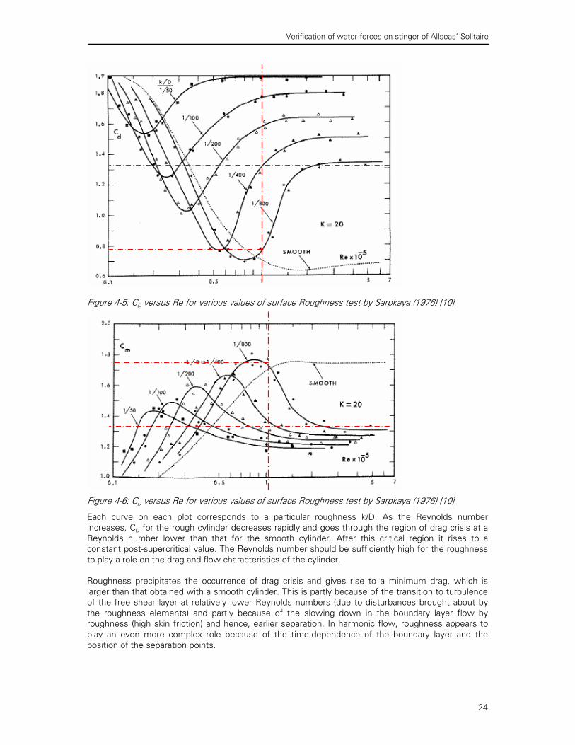
experiments with sand-roughened cylinder in harmonic flow (Figures 4-5 and 4-6).
Verification of water forces on stinger of Allseas’ Solitaire
24
Figure 4-5: CD versus Re for various values of surface Roughness test by Sarpkaya (1976) [10]
Figure 4-6: CD versus Re for various values of surface Roughness test by Sarpkaya (1976) [10]
Each curve on each plot corresponds to a particular roughness k/D. As the Reynolds number
increases, CD for the rough cylinder decreases rapidly and goes through the region of drag crisis at a
Reynolds number lower than that for the smooth cylinder. After this critical region it rises to a
constant post-supercritical value. The Reynolds number should be sufficiently high for the roughness
to play a role on the drag and flow characteristics of the cylinder.
Roughness precipitates the occurrence of drag crisis and gives rise to a minimum drag, which is
larger than that obtained with a smooth cylinder. This is partly because of the transition to turbulence
of the free shear layer at relatively lower Reynolds numbers (due to disturbances brought about by
the roughness elements) and partly because of the slowing down in the boundary layer flow by
roughness (high skin friction) and hence, earlier separation. In harmonic flow, roughness appears to
play an even more complex role because of the time-dependence of the boundary layer and the
position of the separation points.

Verification of water forces on stinger of Allseas’ Solitaire
25
Sarpkaya found that the Reynolds number at which the drag crisis occurs gives rise to an ‘inertia
crisis’. For a given relative roughness, CM rises to a maximum at a Reynolds number, which
corresponds to that at which CD drops to a minimum. When there is a rise in the drag coefficient this
goes in combination with a drop in the inertia coefficient and vice versa. Allseas’s cylinders are coated
and really smooth. However, due to marine fouling the cylinders will become rough. The estimated
roughness of the elements in the stinger will be k/D = 1/800. Looking at the stinger elements and the
tests done by Sarpkaya the following force coefficients can be obtained (Table 4-3). [10]
Coefficient Minimum Maximum
Drag CD 0.78 1.32
Inertia CM 1.32 1.72
Table 4-3: Drag and inertia coefficient with roughness effect
4.4 Influence of effects on force coefficients
4.4.1 Force coefficients in waves
The state of understanding of the assumptions and uncertainties that go into the prediction of fluid
loading on offshore structures is difficult to deal with. People are still inadequate to describe the
complex realities of fluid loading on offshore structures. The inherent instability of the oceans gives
rise to complex waves and forces, which may be different from those assumed to exist for design
purposes. It appears that the forces predicted through the use of a design wave will be larger than
those produced on the structure by a real wave field of comparable characteristics.
As in harmonic and uniformly accelerating flows, Morison’s equation is used for estimating wave-
induced forces on offshore structures. In wave force calculations U is taken as the horizontal
component of the water particle velocity. However, Morison’s equation gave rise to a great deal of
discussion on what values of the two coefficients should be used. Another problem is the difficulty of
accurately measuring the velocity and acceleration to be used in Morison’s equation.
The sea surface in non-linear and irregular sea states causes the waves to originate from a range of
directions. There are several wave theories, which can used in calculating the velocities and
accelerations. These theories deal with two-dimensional waves. However each theory has its own
limitations and ranges of applicability. The combined wave and current flow around a vertical circular
cylinder gives rise to a complex, separated and time-dependent flow. None of the phenomena
described above for a steady current and harmonically flow is possible to describe for a wavy climate.
A lot of experiments are done in real wave climates. Their differences in the test conditions, methods
of measurement and data evaluation do not permit a critical and comparative assessment of the drag
and inertia coefficient obtained in each investigation. Two tests from two researches will be treated
here, just to give an indication of the uncertainties in real wave climate tests. Wiegel, Beebe and
Moon (1957) made real measurements at the Pacific coast for a 6.625-inch cylinder. The wave
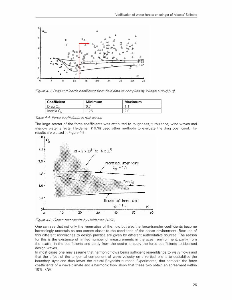
kinematics were determined from linear theory. The results are plotted in Figure 4-7 and the results
are shown in Table 4-4.
Verification of water forces on stinger of Allseas’ Solitaire
26
Figure 4-7: Drag and inertia coefficient from field data as compiled by Wiegel (1957) [10]
Coefficient Minimum Maximum
Drag CD 0.7 1.1
Inertia CM 1.75 2.0
Table 4-4: Force coefficients in real waves
The large scatter of the force coefficients was attributed to roughness, turbulence, wind waves and
shallow water effects. Heideman (1976) used other methods to evaluate the drag coefficient. His
results are plotted in Figure 4-8.
Figure 4-8: Ocean test results by Heideman (1976)
One can see that not only the kinematics of the flow but also the force-transfer coefficients become
increasingly uncertain as one comes closer to the conditions of the ocean environment. Because of
this different approaches to design practice are given by different authoritative sources. The reason
for this is the existence of limited number of measurements in the ocean environment, partly from
the scatter in the coefficients and partly from the desire to apply the force coefficients to idealised
design waves.
In most cases one may assume that harmonic flows bears sufficient resemblance to wavy flows and
that the effect of the tangential component of wave velocity on a vertical pile is to destabilise the
boundary layer and thus lower the critical Reynolds number. Experiments, that compare the force
coefficients of a wave climate and a harmonic flow show that these two obtain an agreement within
10%. [10]

Verification of water forces on stinger of Allseas’ Solitaire
27
4.4.2 Effect of orbital motion
The most importance difference between plane oscillatory flow and real waves is that the water
particles in waves will not follow a straight horizontal line, but will follow an orbital motion due to the
elliptical trajectory. This difference may influence the assumed force on a cylinder. Stansby did
experiments for orbital motion in 1983 and these results are compared with the plane oscillatory flow
results of Sarpkaya (1976). The quantity E is a parameter, which defines the ellipticity of the orbital
motion. VM and UM are the maximum value of the vertical and horizontal components of the particle
velocity (Figure 4-9).
M
M
U
VE = (Eq. 4-3)
CFrms is the force coefficient corresponding to the total in line force. For the lower Reynolds numbers
the scatter is quite large for the drag and inertia coefficient. Looking at the total in line force
coefficient there is a narrow band for E < 0.9. So the total in line force is hardly influenced by the
orbital motion in comparison with the plane oscillatory flow unless the ellipticity exceed values of
about 0.75. A reduction of about 20% to 30% of the total in line force is founded for the values of E
above 0.75. For the large Reynolds numbers, only the range 0.11 — 0.65 for E is investigated. It is
seen that the coefficients do not show a lot of difference between orbital motion and the plane
oscillatory flow. [5]
Figure 4-9: Orbital motion effect on force coefficients [6]

Verification of water forces on stinger of Allseas’ Solitaire
28
4.4.3 Effect of angle of attack on force coefficients
One can imagine the angle in which the cylinder is placed relative to the flow will have influence on
the forces. In most cases people assume that the independence cross-flow principle is applicable.
This principle consists of the assumption that the component of the force normal to the cylinder may
be calculated from the velocity component normal to the cylinder axis (Figure 4-10). This way the drag
coefficient can be taken as in a normal case, so CD is independent of the angel of attack, θ.
ν
DU N
N =Re (Eq. 4-4)
θ
U
UN
90°
Figure 4-10: Independent cross flow principle
If one looks logical, it may be assumed that the flow sees an elliptical cross section if the flow
approaches with an angle. This elliptical form may delay the separation, which results in a different
drag coefficient. Experiments showed that for a cylinder under an angle with the flow the streamlines
in the neighbourhood of the cylinder are bent in such a way that the actual flow at the cylinder is at an
angle of 90 degrees. This means that the flow will not see an elliptical form, but the normal circular
form. So again the drag coefficient is independent of the angle of attack. [5]
However, experiments showed that this independence principle is not applicable beyond the point of
separation and only holds for low Reynolds numbers. The drag coefficient in this principle should not
be taken as usual. Besides, the elliptic cross section will cause a narrower wake, what implies a lower
Strouhal number. This phenomenon was tested by Shirakashi (1986)(Figure 4-11) and proved the
assumption.
Figure 4-11: Frequency of eddy shedding in terms of V, Shirakashi (1986)[11]
For Reynolds number in the range of 2*104 Hayashi (Figure 4-12) did some experiments to measure
the drag coefficient variation independent of the angle of attack.
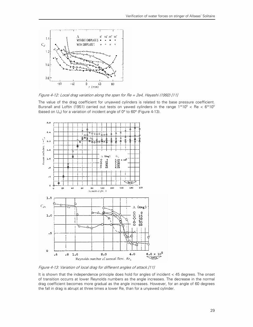
Verification of water forces on stinger of Allseas’ Solitaire
29
Figure 4-12: Local drag variation along the span for Re = 2e4, Hayashi (1992) [11]
The value of the drag coefficient for unyawed cylinders is related to the base pressure coefficient.
Bursnall and Loftin (1951) carried out tests on yawed cylinders in the range 1*105 < Re < 6*105
(based on UN) for a variation of incident angle of 0° to 60° (Figure 4-13).
Figure 4-13: Variation of local drag for different angles of attack.[11]
It is shown that the independence principle does hold for angles of incident < 45 degrees. The onset
of transition occurrs at lower Reynolds numbers as the angle increases. The decrease in the normal
drag coefficient becomes more gradual as the angle increases. However, for an angle of 60 degrees
the fall in drag is abrupt at three times a lower Re, than for a unyawed cylinder.
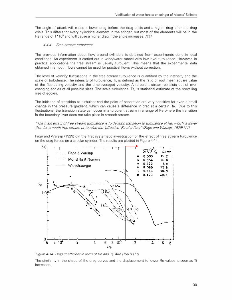
Verification of water forces on stinger of Allseas’ Solitaire
30
The angle of attack will cause a lower drag before the drag crisis and a higher drag after the drag
crisis. This differs for every cylindrical element in the stinger, but most of the elements will be in the
Re range of 1*105 and will cause a higher drag if the angle increases. [11]
4.4.4 Free stream turbulence
The previous information about flow around cylinders is obtained from experiments done in ideal
conditions. An experiment is carried out in wind/water tunnel with low-level turbulence. However, in
practical applications the free stream is usually turbulent. This means that the experimental data
obtained in smooth flows cannot be used for practical flows without correction.
The level of velocity fluctuations in the free stream turbulence is quantified by the intensity and the
scale of turbulence. The intensity of turbulence, Ti, is defined as the ratio of root mean square value
of the fluctuating velocity and the time-averaged velocity. A turbulent stream consists out of ever
changing eddies of all possible sizes. The scale turbulence, Ts, is statistical estimate of the prevailing
size of eddies.
The initiation of transition to turbulent and the point of separation are very sensitive for even a small
change in the pressure gradient, which can cause a difference in drag at a certain Re. Due to this
fluctuations, the transition state can occur in a turbulent stream in a range of Re where the transition
in the boundary layer does not take place in smooth stream.
“The main effect of free stream turbulence is to develop transition to turbulence at Re, which is lower than for smooth free stream or to raise the ‘effective’ Re of a flow” (Fage and Warsap, 1929) [11] Fage and Warsap (1929) did the first systematic investigation of the effect of free stream turbulence
on the drag forces on a circular cylinder. The results are plotted in Figure 4-14.
Figure 4-14: Drag coefficient in term of Re and Ti, Arie (1981) [11]
The similarity in the shape of the drag curves and the displacement to lower Re values is seen as Ti
increases.
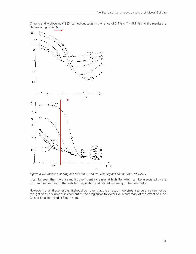
Verification of water forces on stinger of Allseas’ Solitaire
31
Cheung and Melbourne (1983) carried out tests in the range of 0.4% < Ti < 9.1 % and the results are
shown in Figure 4-15.
Figure 4-15: Variation of drag and lift with Ti and Re, Cheung and Melbourne (1983)[12]
It can be seen that the drag and lift coefficient increases at high Re, which can be associated by the
upstream movement of the turbulent separation and related widening of the near wake.
However, for all these results, it should be noted that the effect of free stream turbulence can not be
thought of as a simple displacement of the drag curve to lower Re. A summary of the effect of Ti on
Cd and St is compiled in Figure 4-16.

Verification of water forces on stinger of Allseas’ Solitaire
32
Figure 4-16: Compilation of drag affected by Re and Ti [12]
From the results of the done experiments it can be said that the free stream turbulence will have a lot
of influence. It will take care of a drag crisis to happen at a lower Re. However in case of the stinger
the Reynolds numbers will already be beyond the drag crisis. The main affect of the free stream
turbulence will be a higher drag coefficient for the same Re. [12]
4.4.5 Free ends
The flow around the free end of a finite cylinder will be certainly different then the ‘normal’ flow
around a cylinder. For finite cylinder, there is no physical boundary between free stream pressure and
the base pressure at the free end. The considerable pressure difference will induce a secondary flow
over the free end into the near wake. A flow visualisation of the flow around a free end is done by
Slaouti and Gerrard (1981) in Figure 4-17.
Figure 4-17: Flow visualisation around free end [11]
Wieselberger (1922) did the earliest experiments on finite circular cylinders with two free ends. His
experiment went up to Re = 8.105 and shows in Figure 4-18 the drag coefficient against L/D = 5 and
L/D = ∞ in term of Re. ( L is the length of the cylinder)
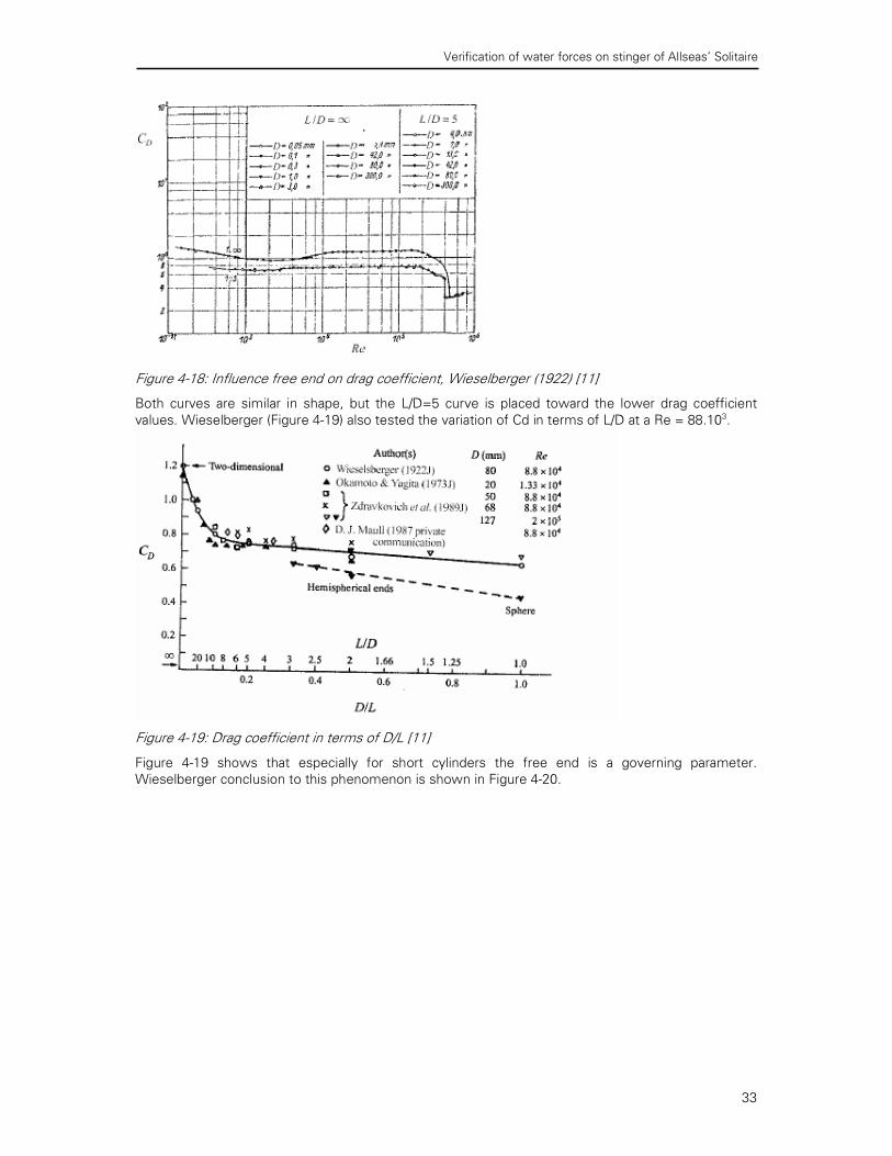
Verification of water forces on stinger of Allseas’ Solitaire
33
Figure 4-18: Influence free end on drag coefficient, Wieselberger (1922) [11]
Both curves are similar in shape, but the L/D=5 curve is placed toward the lower drag coefficient
values. Wieselberger (Figure 4-19) also tested the variation of Cd in terms of L/D at a Re = 88.103.
Figure 4-19: Drag coefficient in terms of D/L [11]
Figure 4-19 shows that especially for short cylinders the free end is a governing parameter.
Wieselberger conclusion to this phenomenon is shown in Figure 4-20.

Verification of water forces on stinger of Allseas’ Solitaire
34
Figure 4-20: Flow phenomenon around two free end cylinder [11]
“The explanation for the fall in drag coefficient with decreasing aspect ratio should be sought in the venting of a dead water (near wake) behind a buff body; an inflow of the fluid into the near wake space on its way around the cylinder ends. Hence, the pressure over the back side of the body would rise, and so the drag would be smaller.” (Wieselberger) [11] In the case of the stinger, all the cylindrical elements are respectively long and the shortest element
is L/D > 15. This means that the free ends phenomenon will not pay a severe role in the stinger. [11]
4.5 Interference of two cylinders
A body’s resistance to flow is strongly affected by what surrounds it. When two bodies are near each
other the flow around the two bodies will be affected. This situation is certainly present in the case of
the stinger, which consist out of several tubes in different arrangements. For a certain flow condition,
the quantification of the interference effects in terms of the pressure distribution, lift and drag forces
and vortex shedding frequency is the essence of the problem.
A very important feature in determining the flow around the cylinder elements of the stinger is the
influence of cylinder elements on each other. First the simplest form will be taken into consideration,
which consists only out of 2 circular cylinder elements.
Two parallel circular cylinders placed close to each other have been employed in many areas of
engineering. The first assumption of people was that the flow around two cylinders would be the
same as for a single cylinder and that the interference effect was negligible. But some tests showed
immediately that it might cause considerable changes into flow patterns and the magnitude of forces.
The interference effects strongly depend on the arrangement of the two cylinders and their
orientation to the free stream. Zdravkovich (1977) adopts three simple categories (Figure 4-21):
(i) T, the tandem arrangement; one cylinder behind the other relative to the free stream.
(ii) SS, the side-by-side arrangement; both cylinders face the free stream;
(iii) S, the staggered arrangement; the cylinders are at any combination of streamwise
S/D and transverse T/D spacing ratio components.
Error!
Figure 4-21: Arrangements for a pair of cylinders
(i) (ii) (iii)
U U U
Y
X
S
α = 0 α= 90 0 < α < 90 T
S
α
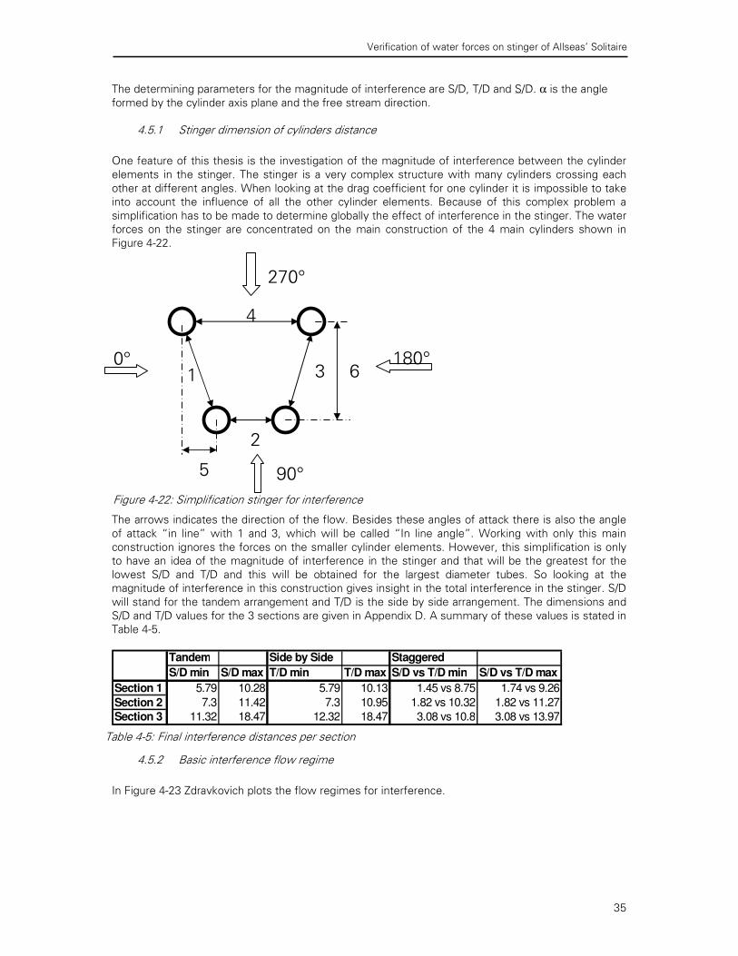
Verification of water forces on stinger of Allseas’ Solitaire
35
The determining parameters for the magnitude of interference are S/D, T/D and S/D. α is the angle
formed by the cylinder axis plane and the free stream direction.
4.5.1 Stinger dimension of cylinders distance
One feature of this thesis is the investigation of the magnitude of interference between the cylinder
elements in the stinger. The stinger is a very complex structure with many cylinders crossing each
other at different angles. When looking at the drag coefficient for one cylinder it is impossible to take
into account the influence of all the other cylinder elements. Because of this complex problem a
simplification has to be made to determine globally the effect of interference in the stinger. The water
forces on the stinger are concentrated on the main construction of the 4 main cylinders shown in
Figure 4-22.
The arrows indicates the direction of the flow. Besides these angles of attack there is also the angle
of attack “in line” with 1 and 3, which will be called “In line angle”. Working with only this main
construction ignores the forces on the smaller cylinder elements. However, this simplification is only
to have an idea of the magnitude of interference in the stinger and that will be the greatest for the
lowest S/D and T/D and this will be obtained for the largest diameter tubes. So looking at the
magnitude of interference in this construction gives insight in the total interference in the stinger. S/D
will stand for the tandem arrangement and T/D is the side by side arrangement. The dimensions and
S/D and T/D values for the 3 sections are given in Appendix D. A summary of these values is stated in
Table 4-5.
Tandem Side by Side Staggered
S/D min S/D max T/D min T/D max S/D vs T/D min S/D vs T/D max
Section 1 5.79 10.28 5.79 10.13 1.45 vs 8.75 1.74 vs 9.26
Section 2 7.3 11.42 7.3 10.95 1.82 vs 10.32 1.82 vs 11.27
Section 3 11.32 18.47 12.32 18.47 3.08 vs 10.8 3.08 vs 13.97
4.5.2 Basic interference flow regime
In Figure 4-23 Zdravkovich plots the flow regimes for interference.
4
2
3 6
5
1 0° 180°
90°
270°
Figure 4-22: Simplification stinger for interference
Table 4-5: Final interference distances per section
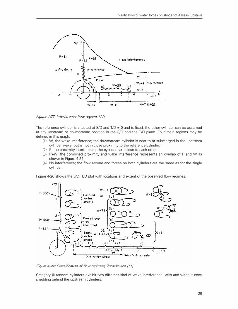
Verification of water forces on stinger of Allseas’ Solitaire
36
Figure 4-23: Interference flow regions [11]
The reference cylinder is situated at S/D and T/D = 0 and is fixed, the other cylinder can be assumed
at any upstream or downstream position in the S/D and the T/D plane. Four main regions may be
defined in this graph:
(1) W, the wake interference; the downstream cylinder is near to or submerged in the upstream
cylinder wake, but is not in close proximity to the reference cylinder;
(2) P, the proximity interference; the cylinders are close to each other
(3) P+W, the combined proximity and wake interference represents an overlap of P and W as
shown in Figure 4-24
(4) No interference; the flow around and forces on both cylinders are the same as for the single
cylinder.
Figure 4-26 shows the S/D, T/D plot with locations and extent of the observed flow regimes.
Figure 4-24: Classification of flow regimes, Zdravkovich [11]
Category (i) tandem cylinders exhibit two different kind of wake interference: with and without eddy
shedding behind the upstream cylinders:
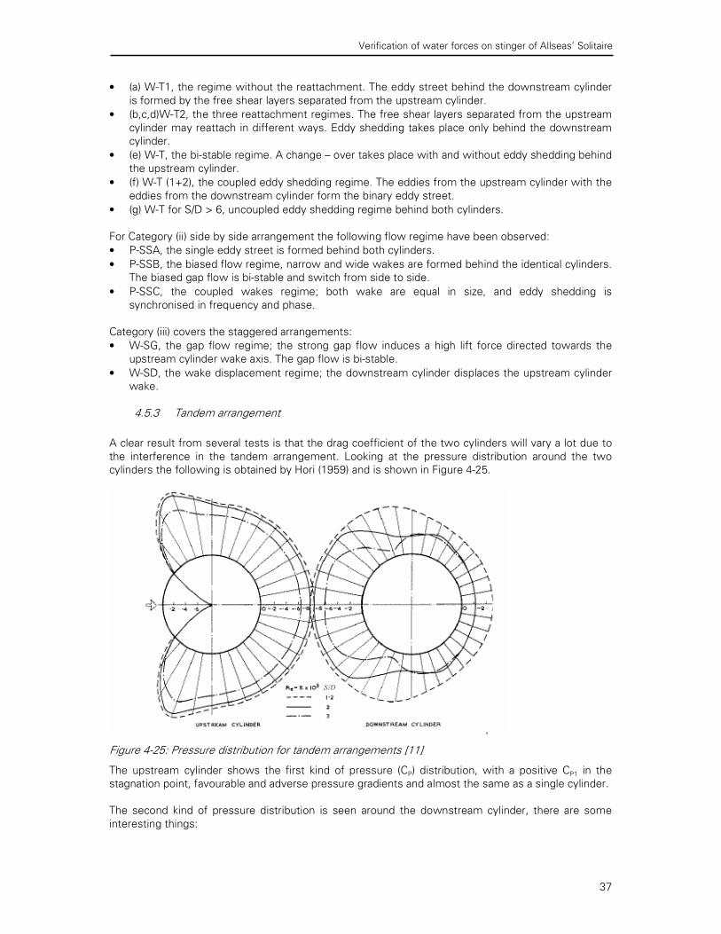
Verification of water forces on stinger of Allseas’ Solitaire
37
• (a) W-T1, the regime without the reattachment. The eddy street behind the downstream cylinder
is formed by the free shear layers separated from the upstream cylinder.
• (b,c,d)W-T2, the three reattachment regimes. The free shear layers separated from the upstream
cylinder may reattach in different ways. Eddy shedding takes place only behind the downstream
cylinder.
• (e) W-T, the bi-stable regime. A change — over takes place with and without eddy shedding behind
the upstream cylinder.
• (f) W-T (1+2), the coupled eddy shedding regime. The eddies from the upstream cylinder with the
eddies from the downstream cylinder form the binary eddy street.
• (g) W-T for S/D > 6, uncoupled eddy shedding regime behind both cylinders.
For Category (ii) side by side arrangement the following flow regime have been observed:
• P-SSA, the single eddy street is formed behind both cylinders.
• P-SSB, the biased flow regime, narrow and wide wakes are formed behind the identical cylinders.
The biased gap flow is bi-stable and switch from side to side.
• P-SSC, the coupled wakes regime; both wake are equal in size, and eddy shedding is
synchronised in frequency and phase.
Category (iii) covers the staggered arrangements:
• W-SG, the gap flow regime; the strong gap flow induces a high lift force directed towards the
upstream cylinder wake axis. The gap flow is bi-stable.
• W-SD, the wake displacement regime; the downstream cylinder displaces the upstream cylinder
wake.
4.5.3 Tandem arrangement
A clear result from several tests is that the drag coefficient of the two cylinders will vary a lot due to
the interference in the tandem arrangement. Looking at the pressure distribution around the two
cylinders the following is obtained by Hori (1959) and is shown in Figure 4-25.
Figure 4-25: Pressure distribution for tandem arrangements [11]
The upstream cylinder shows the first kind of pressure (CP) distribution, with a positive CP1 in the
stagnation point, favourable and adverse pressure gradients and almost the same as a single cylinder.
The second kind of pressure distribution is seen around the downstream cylinder, there are some
interesting things:

Verification of water forces on stinger of Allseas’ Solitaire
38
• The base pressure behind the upstream cylinder faces the upstream side of the gap and the gap
pressure is exerted along the front side of the downstream cylinder
• The gap pressure is lower than the base pressure, which indicates in a negative CD2. This means
that the drag for the second cylinder is directed in negative direction against the drag of the first
cylinder. This results in a lower overall drag for the tandem arrangement.
Igarashi (1981) carried out extensive pressure distribution measurements around tandem cylinders in
terms of S/D and Re. The results of these tests are plotted in Figure 4-26.
Figure 4-26: Mean pressure distribution (a) Front cylinder, (b) rear cylinder [11]
The interference affects only the pressure distribution at the backside for the first cylinder. For the
second cylinder the pressure distribution curves are plotted in the right Figure.
Several measurements are done by different people and Zdravkovich (1977) compiled all these data
into a single plot of CD1 and CD2 in term of S/D and Re in Figure 4-27. The closed symbols are the drag
coefficients of the first cylinder and the open symbols of the second cylinder.

Verification of water forces on stinger of Allseas’ Solitaire
39
Figure 4-27: Compilation of drag coefficients for tandem arrangements in terms of S/D and Re. [11]
Figure 4-27 shows the following trends:
• There is a strong Re effect on the CD2 curves. For S/D < 3.5 the drag coefficient is negative and
acts as a thrust force. For S/D > 3.5 it becomes positive for high Re.
• The variation in CD2 reflects the effect of the upstream wake turbulence on the flow past the
downstream cylinder.
For the stinger the influence of interference on the drag coefficient can be obtained for the different
sections. For section 1 a S/D = 5.8 is found; working with a Re of 1.6*105 to 1.3*106 this result in a
drag coefficient for the downstream cylinder of CD2 = 0.21 — 0.28. This is a significant difference
comparing with the first assumption of CD2 = 1.2. For higher S/D till 10 the drag coefficient for the
downstream cylinder remains the same, but for much higher S/D and higher Re there are no test
results available. However it may be assumed that the drag coefficient will definitely be reduced due
to interference. The S/D in section 2 and 3 is most of the times higher then 10.

Verification of water forces on stinger of Allseas’ Solitaire
40
There are no results for these values, but the drag coefficient will increase again with increasing the
S/D value. It is assumed that after S/D > 20 the drag coefficient for the downstream cylinder will be
the same as for a single cylinder. This means that the interference in the stinger will definitely result
in a lower drag. The flow regimes discussed earlier are only applicable for the upstream cylinder. The
downstream cylinder is submerged into the turbulent wake, which affect transition and separation.
Okajima (1977) carried out tests on tandem cylinder for 1 < S/D < 6.5 and 4*104 < Re < 6.3*105.
Figure 4-28 shows the drag coefficient for the upstream and downstream cylinder for only S/D = 3
and 5.
Figure 4-28: Tandem cylinder, drag coefficient vs Re [11]
It can be seen that the drag coefficient of the upstream cylinder decreases with the drag crisis, but at
that moment, the drag coefficient of the downstream cylinder increases. However, it is remains
constant after this crisis, what results in a drag coefficient of 0.5. This results again in a lower total
drag for the tandem arrangement in comparison with the approach of every element separately.
The free stream turbulence acts as a random and three-dimensional unsteady perturbation. The
transition in the boundary and free shear layers is promoted at lower Re than in smooth flow. The free
stream turbulence enhances mixing, entrainment and turbulent diffusion. These remarks are pertinent
to the upstream cylinder, while the downstream cylinder is already submerged in the turbulent wake.
Tandem cylinders are separated by a gap, which is bounded by the free shear layers. The gap can be
thought of as a wake of restricted length and the free stream turbulence triggers an early transition in
the free shear layers. The expected result is an early start of eddy shedding behind the upstream
cylinder at smaller S/D (Figure 4-29)
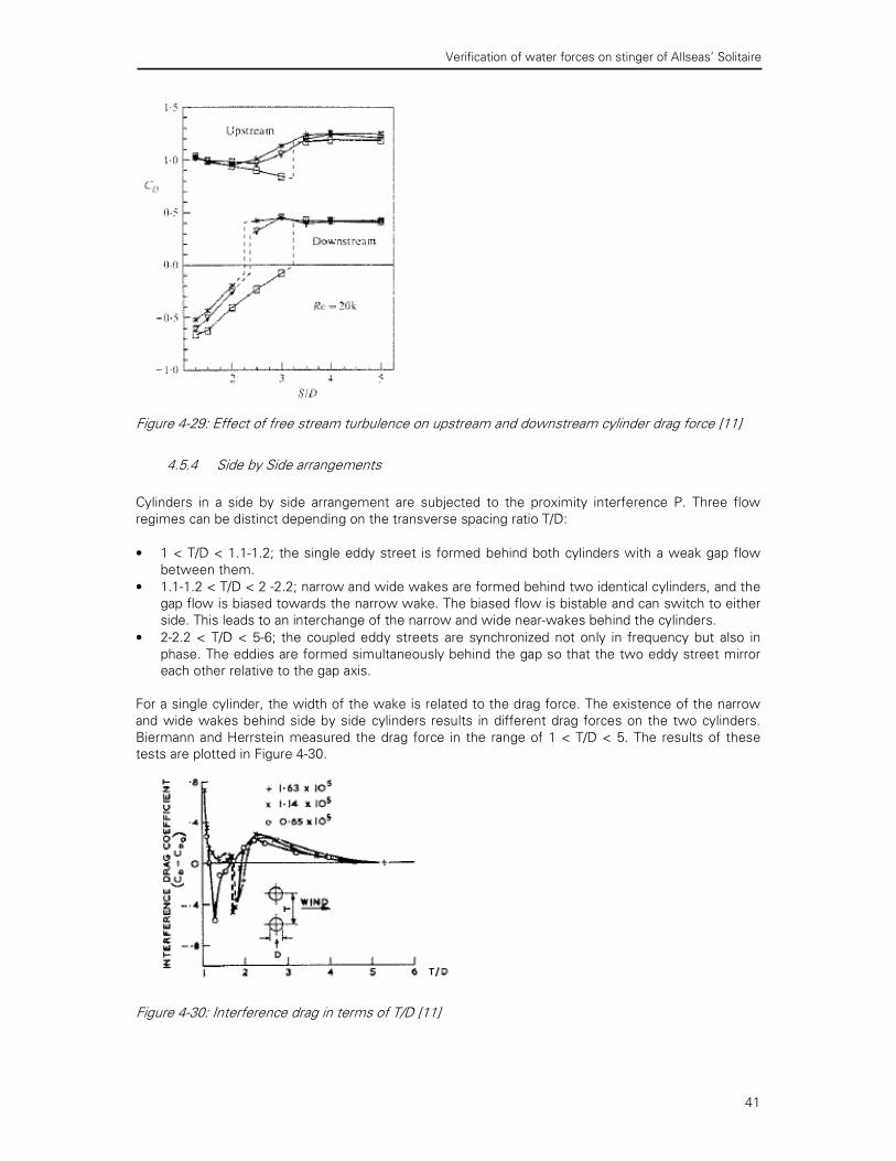
Verification of water forces on stinger of Allseas’ Solitaire
41
Figure 4-29: Effect of free stream turbulence on upstream and downstream cylinder drag force [11]
4.5.4 Side by Side arrangements
Cylinders in a side by side arrangement are subjected to the proximity interference P. Three flow
regimes can be distinct depending on the transverse spacing ratio T/D:
• 1 < T/D < 1.1-1.2; the single eddy street is formed behind both cylinders with a weak gap flow
between them.
• 1.1-1.2 < T/D < 2 -2.2; narrow and wide wakes are formed behind two identical cylinders, and the
gap flow is biased towards the narrow wake. The biased flow is bistable and can switch to either
side. This leads to an interchange of the narrow and wide near-wakes behind the cylinders.
• 2-2.2 < T/D < 5-6; the coupled eddy streets are synchronized not only in frequency but also in
phase. The eddies are formed simultaneously behind the gap so that the two eddy street mirror
each other relative to the gap axis.
For a single cylinder, the width of the wake is related to the drag force. The existence of the narrow
and wide wakes behind side by side cylinders results in different drag forces on the two cylinders.
Biermann and Herrstein measured the drag force in the range of 1 < T/D < 5. The results of these
tests are plotted in Figure 4-30.
Figure 4-30: Interference drag in terms of T/D [11]

Verification of water forces on stinger of Allseas’ Solitaire
42
The lowest T/D value obtained in the stinger is T/D =5.8, looking at Figure 5-31 it can be said that the
side by side interference is not really present in the stinger. For T/D < 5 the drag coefficient starts to
increase, and reaches a maximum at T/D =2.2 in the P-SS regime. A compilation of the obtained
results, produced a graph were the drag coefficient and the lift coefficient are viewed against T/D at
several Re (Figure 4-33)
Figure 4-31: Drag and lift in terms of T/D [11]
Again the drag and lift coefficient changes due to interference of the side by side arrangement will
not hold for the present case of the stinger. The movement of the stagnation point due to the
proximity of the other cylinder rotates the resultant force vector towards the gap, thus producing the
component in the lift direction. Figure 4-31 also clearly shows the variation in CL in terms of T/D.
4.5.5 Staggered arrangements
Staggered arrangements have often occurred in many engineering applications but have attracted
less research in comparison with tandem and side by side arrangements. The common feature of all
spacings is the narrow and wide wakes behind the upstream and downstream cylinders. The bigger
the spacing, the less is the bias is of the gap flow and the differences in size of the two wakes.
Zdravkovich (1977) compiled in Figure 4-32 the result of several measurements and displaced these
results in a T/D and S/D plane.
Figure 4-32: Drag and lift in the S/D and T/D plane [11]

Verification of water forces on stinger of Allseas’ Solitaire
43
Zdravkovich (1977) suggested that the following magnitude and sign of the lift coefficient should be
used as a criterion for the classification of staggered arrangements:
(1) CL = 0, the upstream cylinder is in the upstream proximity region in tandem arrangements or
in the no interference region
(2) CL > 0, the side proximity region; the repulsive lift force and the increased or decreased drag
force
(3) CL < 0, the wake interference region; the attractive lift force and the increased or decreased
drag force.
Based on the previous information the stinger will notice no interference for its staggered cylinder
arrangement. [11]
4.6 Vortex shedding
On vortex shedding and the resulting alternating force in a steady flow there have been done
extensive studies. Lift forces are important not only because of their magnitude but also because of
their alternating nature, which may lead to vortex synchronisation. This transverse force is also
measured by the experiments of Sarpkaya (1976) and shown in Figures 4-33 and 4-34.
Figure 4-33: CL versus versus KC for various values Re tests by T. Sarpkaya (1976) [10]
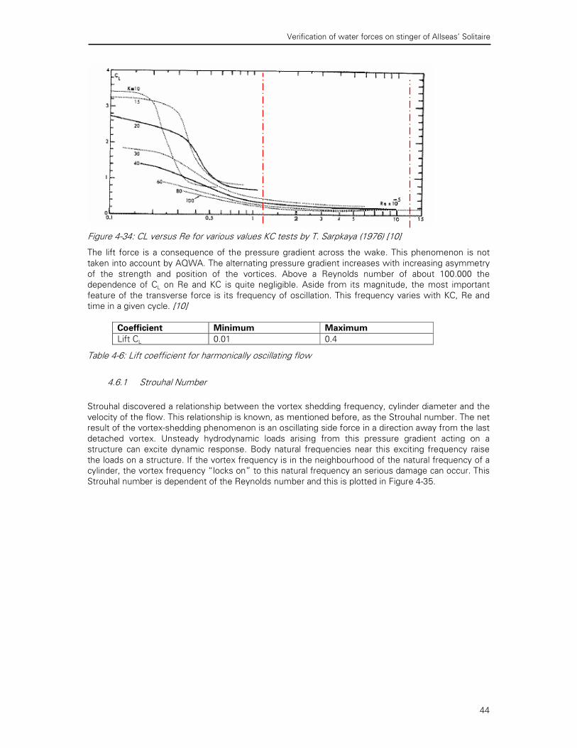
Verification of water forces on stinger of Allseas’ Solitaire
44
Figure 4-34: CL versus Re for various values KC tests by T. Sarpkaya (1976) [10]
The lift force is a consequence of the pressure gradient across the wake. This phenomenon is not
taken into account by AQWA. The alternating pressure gradient increases with increasing asymmetry
of the strength and position of the vortices. Above a Reynolds number of about 100.000 the
dependence of CL on Re and KC is quite negligible. Aside from its magnitude, the most important
feature of the transverse force is its frequency of oscillation. This frequency varies with KC, Re and
time in a given cycle. [10]
Coefficient Minimum Maximum
Lift CL 0.01 0.4
Table 4-6: Lift coefficient for harmonically oscillating flow
4.6.1 Strouhal Number
Strouhal discovered a relationship between the vortex shedding frequency, cylinder diameter and the
velocity of the flow. This relationship is known, as mentioned before, as the Strouhal number. The net
result of the vortex-shedding phenomenon is an oscillating side force in a direction away from the last
detached vortex. Unsteady hydrodynamic loads arising from this pressure gradient acting on a
structure can excite dynamic response. Body natural frequencies near this exciting frequency raise
the loads on a structure. If the vortex frequency is in the neighbourhood of the natural frequency of a
cylinder, the vortex frequency “locks on” to this natural frequency an serious damage can occur. This
Strouhal number is dependent of the Reynolds number and this is plotted in Figure 4-35.

Verification of water forces on stinger of Allseas’ Solitaire
45
Figure 4-35: Strouhal number against Reynolds number [6]
For the stinger the Strouhal number will be in the range of 0.18 — 0.3. This means that the range of
vortex frequencies will be 0.615 - 1.73 Hz.
4.7 Final differences
In this chapter all the possible effects that can cause a difference between AQWA and reality has
been investigated.
Possible causes for differences are:
i. Drag coefficient ≠ 1.2 ii. Force coefficient in waves — orbital motion
iii. Angle of Attack
iv. Free stream turbulence
v. Free ends
vi. Interference
vii. Vortex shedding
For all the causes their effect on the force coefficient was examined.
i. Allseas works with a drag coefficient of 1.2 in AQWA. This value is obtained form results of the
Sarpkaya experiment executed with rough pipes. For a increased roughness height of only 1
mm there will already be a huge increase of the drag coefficient. The stinger will get rough due
to marine fouling, so the drag coefficient can increase drastically if the cylindrical elements
become rough.
ii. There are too many non-linearities in ocean waves to determine the force coefficients for a
certain sea state. There are tests done for orbital motion to approach the real waves. Based on
these experiments it may be concluded that for taking into account the orbital motion, the total
in line forces is practically uninfluenced for the ellipticity range of E < 0.7. If the ellipticity may
exceed this value the total in line force will experience a reduction of about 20 —30%, with
respect to the measured plane oscillatory in line force results. However due the non-linearities
in ocean waves it is impossible to determine the influence on the force coefficients. The orbital
motion approach can figure as an indication that it will not cause higher forces, but this effect of
waves will not be taken into account further in this thesis.
iii. From test results it is seen that the angle of attack will not have a lot of influence on the drag
and inertia coefficient if the Reynolds number is significant low. For these low Reynolds

Verification of water forces on stinger of Allseas’ Solitaire
46
numbers the independence principle will be valid. However, for high Reynolds numbers this
principle will not hold. The normal drag coefficient can not be taken from the known graphs as
is assumed in the independence principle. From experiments, it follows that the drag
coefficient is of a higher value if the angle of attack increases. AQWA calculates within the
Morison formula with the velocity and acceleration perpendicular to the tube axis, but also with
the usual ‘normal’ drag coefficient. This is proved wrong by experiments and can cause a
difference between the MARIN and AQWA results.
iv. Free stream turbulence can have a great influence on the drag and inertia coefficient. However,
it is very important in what range of Re one is looking. If it is before the drag crisis the free
stream turbulence will result in a lower drag and inertia, but the inverse holds for beyond the
drag crisis. The range of Re in case of the stinger varies a lot, but is most of the time beyond
the drag crisis. Therefore this effect should be taken into account when comparing with reality.
v. It is described in paragraph 4.4.5 that free ends can reduce the drag force. However, all the
free ends will reduce the drag but will also increase the free stream turbulence. In the stinger
there are only a few free ends and these will not reduce the drag coefficient severely. This
phenomenon will not be taken into account for the difference between AQWA and real life.
vi. In this chapter the magnitude of interference in the stinger was looked at. First the stinger was
very roughly simplified to a simple construction, which presented the most important elements
in the stinger, to get an idea of the magnitude of interference. During this investigation, the
conclusion arises that cylinders, which are in side by side and staggered arrangements in the
stinger will not be influenced by each other. However, the cylinder elements, which are in
tandem arrangement in the stinger, will be definitely influenced by each other. From results
obtained by experiments it is possible to define a lower drag coefficient for the downstream
cylinder. Which cylinder in the stinger is the downstream or upstream cylinder depends from
which direction the stream is coming. The drag coefficient can reduce to 0.21 — 0.50, which is a
huge decrease of the drag coefficient and this can be one of the major differences between
AQWA and the MARIN model.
vii. Vortex shedding is a phenomenon that is not taken into account in AQWA. It is described in
paragraph 4.6 that there will definitely be vortex shedding around the cylindrical elements in the
stinger.
From this summary it can be concluded that the main differences between AQWA and the processes
in the prototype can be assigned to the following features:
• Angle of Attack
• Free stream turbulence
• Interference
• Vortex shedding

Verification of water forces on stinger of Allseas’ Solitaire
47
5 MARIN Tests
5.1 Introduction
In 1993 and 2000 Allseas Engineering commissioned the Maritime Research Institute Netherlands
(“MARIN”) to carry out model tests on the Solitaire. During these tests the forces and moments on
the stinger were determined. The tests were carried out in MARIN’s wave and current basin. A model
of the Solitaire and its stinger was built at scale 1:42. The results of these tests are described in
Report No. 2.11861-1-GT/DT May 1993 [13] and Report No. 15946-1-GT April 2000 [14]. The results of
these tests are the comparison material to verify AQWA.
5.2 Response Amplitude Operator
An important parameter in the comparison of the MARIN results with the AQWA results is the so-
called “Response Amplitude Operator” or “RAO”. This term represents the ratio between input
amplitude of an incoming wave and output amplitude of the motion of a structure (Figure 5-1).
Figure 5-1: Response of Structure [6]
The input amplitude will be the incoming wave amplitude and this wave will give the stinger and
vessel a certain motion. This motion is called the response motion and can be described in the known
ship motions: surge, sway, heave, roll, pitch and yaw. Beside these motions, the force on the
vessel/stinger will also get a certain harmonic motion with amplitude. Dividing this amplitude by the
incoming wave amplitude will give the Force RAO. [6]
)(ωζ a
aF= RAO(kN/m) or )(ω
ζ a
az= RAO(-) (Eq. 5-1)
5.3 Test 1: Report No. 2.11861-1-GT/DT 1993
5.3.1 Test set up
The Solitaire model was constructed out of wood at a scale of 1:42 according to drawings of Allseas.
Before the tests were carried out, the weight distribution was checked in air and in water. In
Appendix E the main dimension of the vessel, the stability data and the weight distribution is shown.
The scale model of the stinger was made of steel, taking into account all the cylinder members,
which are relevant for the hydrodynamic properties of the stinger. Basis of the design were the
drawings found in Appendix B. The circular cylinders in the model were built out of small thin-walled
steel pipes with diameters between 8 and 21 millimeters. The roller boxes were built in the model out
of wood, to take into account their volume on the hydrodynamic forces. For these tests the stinger
was fixed to a radius of 225 meter. At the hinge point, where the stinger is attached to the scale
model vessel, the stinger was connected to a six — component force transducer. With this transducer
it was possible to measure the overall loads on the stinger. The total weight of the stinger amounted
to 493.5 tonne force and the origin of the axis system is at the hinge point.
The hinge is situated 15.875 m above the base. It should be noted that the results presented in this
report are presented with respect to the centre of the transducer, which is 4.64 meters in front of the
real hinge point (figure 5-2). [13]
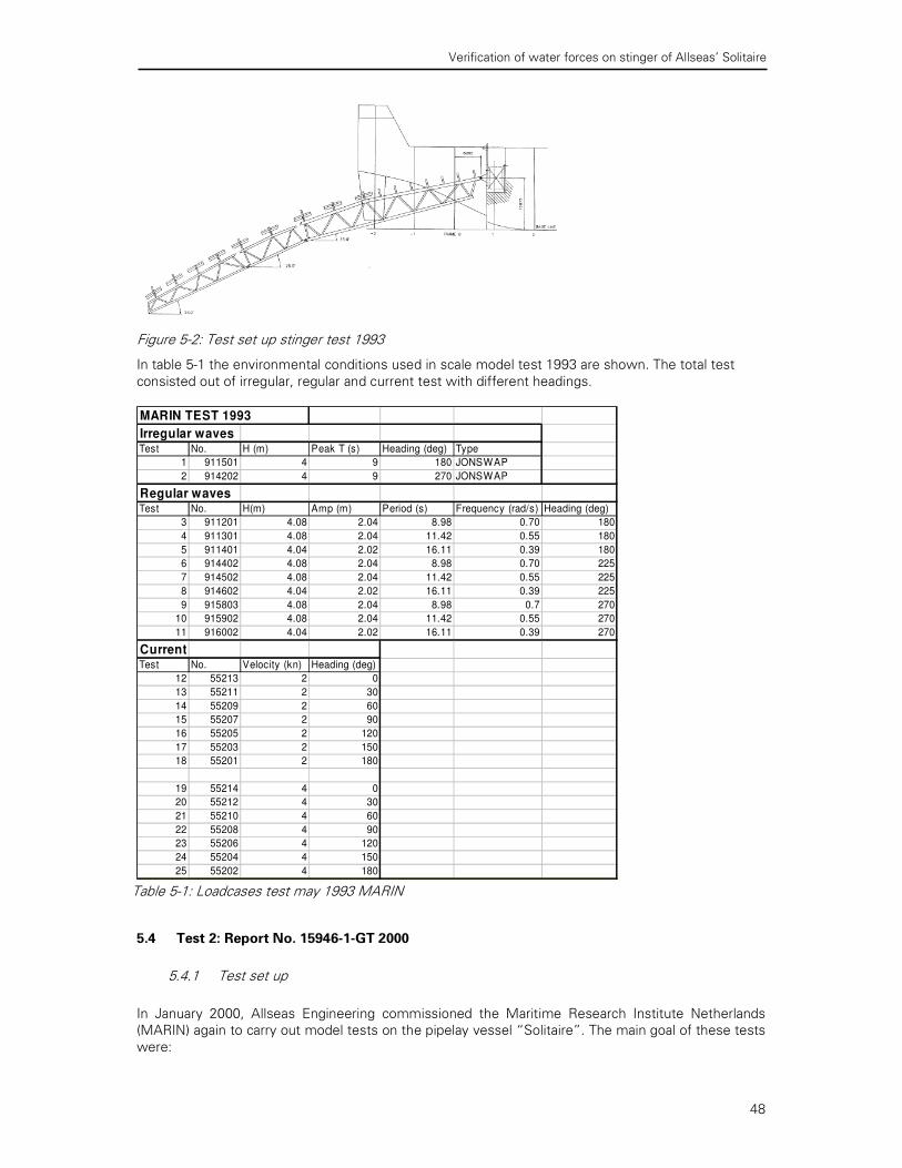
Verification of water forces on stinger of Allseas’ Solitaire
48
Figure 5-2: Test set up stinger test 1993
In table 5-1 the environmental conditions used in scale model test 1993 are shown. The total test
consisted out of irregular, regular and current test with different headings.
MARIN TEST 1993
Irregular wavesTest No. H (m) Peak T (s) Heading (deg) Type
1 911501 4 9 180 JONSWAP
2 914202 4 9 270 JONSWAP
Regular wavesTest No. H(m) Amp (m) Period (s) Frequency (rad/s) Heading (deg)
3 911201 4.08 2.04 8.98 0.70 180
4 911301 4.08 2.04 11.42 0.55 180
5 911401 4.04 2.02 16.11 0.39 180
6 914402 4.08 2.04 8.98 0.70 225
7 914502 4.08 2.04 11.42 0.55 225
8 914602 4.04 2.02 16.11 0.39 225
9 915803 4.08 2.04 8.98 0.7 270
10 915902 4.08 2.04 11.42 0.55 270
11 916002 4.04 2.02 16.11 0.39 270
CurrentTest No. Velocity (kn) Heading (deg)
12 55213 2 0
13 55211 2 30
14 55209 2 60
15 55207 2 90
16 55205 2 120
17 55203 2 150
18 55201 2 180
19 55214 4 0
20 55212 4 30
21 55210 4 60
22 55208 4 90
23 55206 4 120
24 55204 4 150
25 55202 4 180
5.4 Test 2: Report No. 15946-1-GT 2000
5.4.1 Test set up
In January 2000, Allseas Engineering commissioned the Maritime Research Institute Netherlands
(MARIN) again to carry out model tests on the pipelay vessel “Solitaire”. The main goal of these tests
were:
Table 5-1: Loadcases test may 1993 MARIN
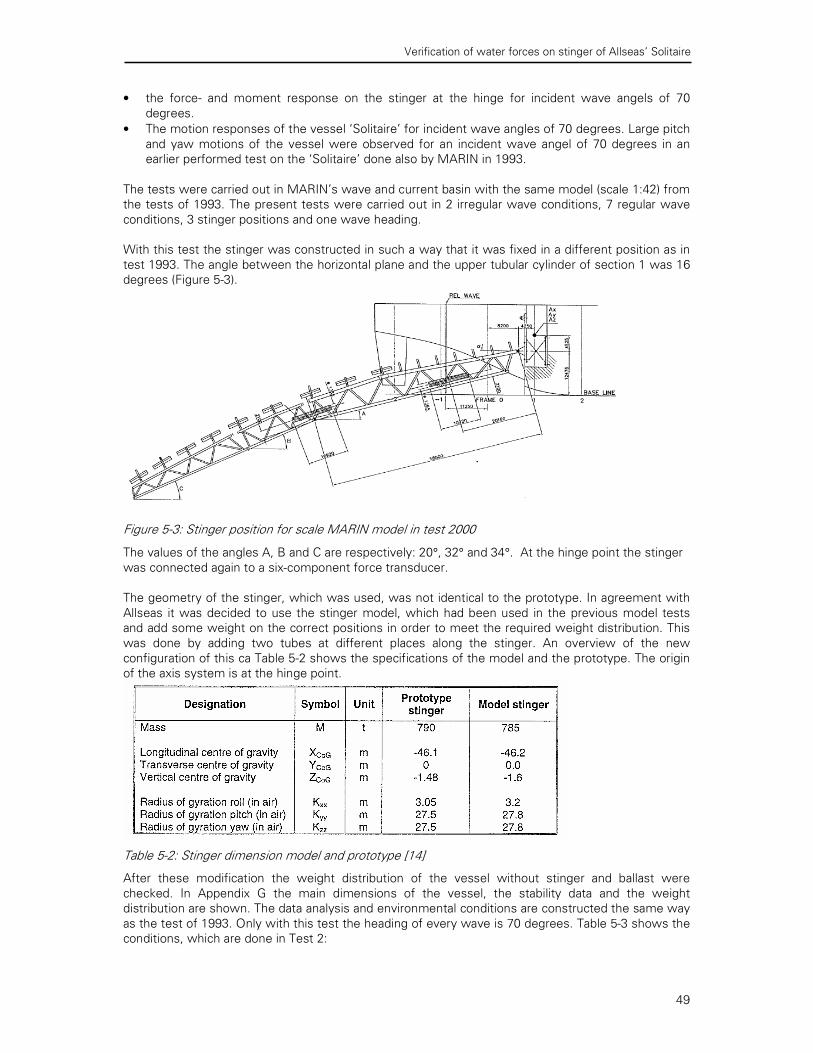
Verification of water forces on stinger of Allseas’ Solitaire
49
• the force- and moment response on the stinger at the hinge for incident wave angels of 70
degrees.
• The motion responses of the vessel ‘Solitaire’ for incident wave angles of 70 degrees. Large pitch
and yaw motions of the vessel were observed for an incident wave angel of 70 degrees in an
earlier performed test on the ‘Solitaire’ done also by MARIN in 1993.
The tests were carried out in MARIN’s wave and current basin with the same model (scale 1:42) from
the tests of 1993. The present tests were carried out in 2 irregular wave conditions, 7 regular wave
conditions, 3 stinger positions and one wave heading.
With this test the stinger was constructed in such a way that it was fixed in a different position as in
test 1993. The angle between the horizontal plane and the upper tubular cylinder of section 1 was 16
degrees (Figure 5-3).
Figure 5-3: Stinger position for scale MARIN model in test 2000
The values of the angles A, B and C are respectively: 20°, 32° and 34°. At the hinge point the stinger
was connected again to a six-component force transducer.
The geometry of the stinger, which was used, was not identical to the prototype. In agreement with
Allseas it was decided to use the stinger model, which had been used in the previous model tests
and add some weight on the correct positions in order to meet the required weight distribution. This
was done by adding two tubes at different places along the stinger. An overview of the new
configuration of this ca Table 5-2 shows the specifications of the model and the prototype. The origin
of the axis system is at the hinge point.
Table 5-2: Stinger dimension model and prototype [14]
After these modification the weight distribution of the vessel without stinger and ballast were
checked. In Appendix G the main dimensions of the vessel, the stability data and the weight
distribution are shown. The data analysis and environmental conditions are constructed the same way
as the test of 1993. Only with this test the heading of every wave is 70 degrees. Table 5-3 shows the
conditions, which are done in Test 2:

Verification of water forces on stinger of Allseas’ Solitaire
50
MARIN TEST 2000Test No. Heading (deg)H (m) Period (s) Frequency (rad/s) Stinger(deg)
26 904009 70 3.8 15 0.419 16
27 904007 70 3.8 10.1 0.622 16
28 904008 70 4.2 9 0.698 16
29 904005 70 4.2 8 0.785 16
30 904004 70 4.7 7 0.898 16
31 904002 70 3.1 6 1.047 16
Irregular wavesTest No. Heading (deg)H (m) Period (s) Spectrum type Stinger (deg)
32 902003 70 4 9 JONSWAP 16
Table 5-3: Load cases test 2000 MARIN
The test set up for this test can be seen in figure 5-4:
Figure 5-4: Test set up test 2000 heading 70 degrees
5.5 Data Analysis
The recording equipment consists out of a ultra-violet light sensitive paper chart recorder and a
magnetic tape recorder, which converts it to a digital form. The results of the measurements were
scaled up to full size values according to Froude’s law of similitude (Appendix F). The results of this
scaling are shown in Table 5-4.
Quantity Scaling Factor Model Prototype
Linear dimensions [m] 42 1 42.00
Volume [m3] 42 3 1 74.008
Angle [°] 1 1 1
Velocity [m/s] 42 0.5 1 6.48
Acceleration [m/s2] 1 1 1
Force [N] ρ 42 3 1 75.940
Table 5-4: Scaling factor at MARIN test
The measured quantities are treated with a statistical analysis according to Figure 5-3:

Verification of water forces on stinger of Allseas’ Solitaire
51
Figure 5-3: Statistical Analysis
1. Mean value −
u (MEAN) ∑=
−
=N
n
nuN
u1
1
2. Standard deviation uσ (ST. DEV) ∑=
−
−=N
n
nu uuN 1
2)(
1σ
3. Maximum value A MAX+ Highest crest value
4. Maximum value A MAX - Highest trough value
Apart form the statistical quantities, another result of the tests in irregular seas is the spectral density
of a signal. The response functions for linear signals are calculated form the spectral densities in the
following way:
)(
)(
)(
)(
e
euu
ea
ea
uS
SuH
ω
ω
ωζ
ω
ζζ
== (Eq. 5-2)
For the regular wave tests, the response functions were calculated by dividing the amplitude of the
first harmonic component of the measured signal by the first harmonic component of the calibrated
wave. For the stinger loads, also response functions are presented and calculated to get some insight
into the trend in the stinger forces and moments.
The measurements of the adjusted wave and stinger loads were subjected to an additional statistical
analysis yielding the crest and trough distributions on Weibull probability paper. These distributions
may be used to predict the probability that a crest exceeds, in this case, a magnitude of 0.1%. An
example of a Weibull AQWA output is given in Figure 5-4.
Figure 5-5: Example Weibull distribution
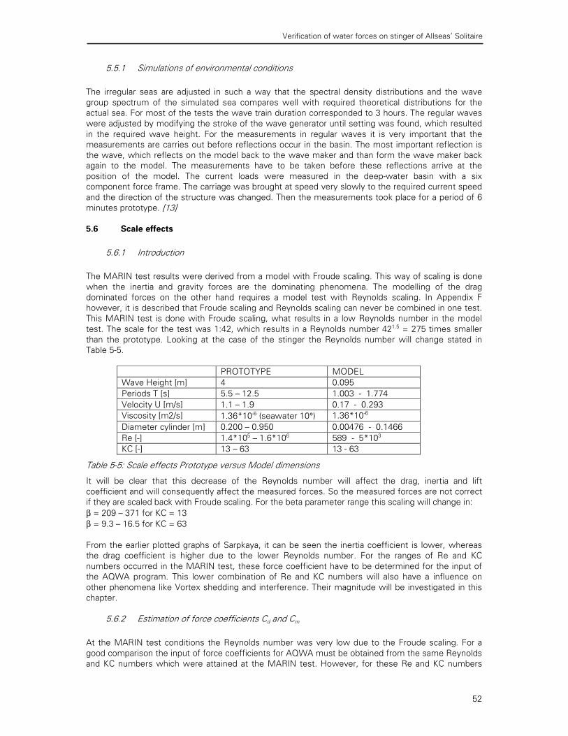
Verification of water forces on stinger of Allseas’ Solitaire
52
5.5.1 Simulations of environmental conditions
The irregular seas are adjusted in such a way that the spectral density distributions and the wave
group spectrum of the simulated sea compares well with required theoretical distributions for the
actual sea. For most of the tests the wave train duration corresponded to 3 hours. The regular waves
were adjusted by modifying the stroke of the wave generator until setting was found, which resulted
in the required wave height. For the measurements in regular waves it is very important that the
measurements are carries out before reflections occur in the basin. The most important reflection is
the wave, which reflects on the model back to the wave maker and than form the wave maker back
again to the model. The measurements have to be taken before these reflections arrive at the
position of the model. The current loads were measured in the deep-water basin with a six
component force frame. The carriage was brought at speed very slowly to the required current speed
and the direction of the structure was changed. Then the measurements took place for a period of 6
minutes prototype. [13]
5.6 Scale effects
5.6.1 Introduction
The MARIN test results were derived from a model with Froude scaling. This way of scaling is done
when the inertia and gravity forces are the dominating phenomena. The modelling of the drag
dominated forces on the other hand requires a model test with Reynolds scaling. In Appendix F
however, it is described that Froude scaling and Reynolds scaling can never be combined in one test.
This MARIN test is done with Froude scaling, what results in a low Reynolds number in the model
test. The scale for the test was 1:42, which results in a Reynolds number 421.5 = 275 times smaller
than the prototype. Looking at the case of the stinger the Reynolds number will change stated in
Table 5-5.
PROTOTYPE MODEL
Wave Height [m] 4 0.095
Periods T [s] 5.5 — 12.5 1.003 - 1.774
Velocity U [m/s] 1.1 — 1.9 0.17 - 0.293
Viscosity [m2/s] 1.36*10-6 (seawater 10°) 1.36*10-6
Diameter cylinder [m] 0.200 — 0.950 0.00476 - 0.1466
Re [-] 1.4*105 — 1.6*106 589 - 5*103
KC [-] 13 — 63 13 - 63
Table 5-5: Scale effects Prototype versus Model dimensions
It will be clear that this decrease of the Reynolds number will affect the drag, inertia and lift
coefficient and will consequently affect the measured forces. So the measured forces are not correct
if they are scaled back with Froude scaling. For the beta parameter range this scaling will change in:
β = 209 — 371 for KC = 13
β = 9.3 — 16.5 for KC = 63
From the earlier plotted graphs of Sarpkaya, it can be seen the inertia coefficient is lower, whereas
the drag coefficient is higher due to the lower Reynolds number. For the ranges of Re and KC
numbers occurred in the MARIN test, these force coefficient have to be determined for the input of
the AQWA program. This lower combination of Re and KC numbers will also have a influence on
other phenomena like Vortex shedding and interference. Their magnitude will be investigated in this
chapter.
5.6.2 Estimation of force coefficients Cd and Cm
At the MARIN test conditions the Reynolds number was very low due to the Froude scaling. For a
good comparison the input of force coefficients for AQWA must be obtained from the same Reynolds
and KC numbers which were attained at the MARIN test. However, for these Re and KC numbers

Verification of water forces on stinger of Allseas’ Solitaire
53
there is not a lot of information available on the magnitude of the force coefficients. This combination
is not of that huge interest that experiments were executed in this range of Re and KC. Nevertheless
there has to be a force coefficient input in AQWA to get a comparison.
Some tests were executed, but the results were not applicable. Based on some assumptions and
extrapolation a rough estimate is made for both the force coefficients. The two methods of
determining the drag and inertia coefficient for MARIN conditions are extrapolation of the Sarpkaya
graphs and experiments done by Kuhtz (1996). Also a quick view is obtained of Stokes and Wang
theory, which is applicable for low KC number.
The graphs by Sarpkaya are plotted before and a summary is seen in Figure 5-7. The combinations of
Re and KC numbers, which are valid for the MARIN test conditions is highlighted by the circles in
these figures.
Figure 5-6: Summary of Sarpkaya experiment results for drag and inertia coefficient [10]
Extrapolation of the force coefficients from the figures above seems to be a very hard task for the
ranges of Re and KC that are wanted. From the above figures it follows that the drag coefficient will
be around 2.0 and that the inertia coefficient will be around 1.0, but still descending steep for lower
Reynolds numbers. Sometimes it seems that the inertia coefficient is below 1 and this means that
the added mass coefficient should be negative. This is beyond the scope of this investigation so it is
assumed that the inertia coefficient will not be below a value of 1.0. From this extrapolation method,
a rough estimate can be made of a Cd 1.9 —2.1 and a Cm of 1.0.

Verification of water forces on stinger of Allseas’ Solitaire
54
In general the force coefficients, Cd and Cm, have to be obtained from experiments or from a
numerical solution. However, at very low KC numbers, an analytical solution is possible for these
coefficients. Stokes and Wang (1968)[15] produced a theoretical analysis, which has the following
form (valid for KC<1):
])(4
1)()[(
2
3
)()(42
2
3
12
13
2
3
2
1
−−
−
−−
−+=
++=
πβπβπβπ
πβπβ
KCC
C
d
m
(Eq. 5-3)
This force coefficient prediction only holds when the flow is attached to the cylinder and is laminar.
Honji (1981) and Sarpkaya (1986) were the first two to report there occurred instability leading to
generation of vortex behind the cylinder at higher KC values. As β increases the vortex structure
appeared at lower KC numbers. This instability gives a rise of the drag coefficient above the prediction
of Wang and Stokes. Experiments showed a doubling of the drag coefficient for low Keulegan Carpenter numbers in comparison with the value predicted by this Stokes — Wang drag coefficient
approach. The Stokes and Wang predictions were in agreement with attached- and laminar flow
conditions, but for turbulent flow the predictions does not coincide with experimental data. Based on
these experiments a new semi empirical formula was proposed by Bearman and Russel:
KCKC
Cd 2
1 ζβ
ζ+= (Eq. 5-4)
with ζ1 = 55 and ζ2 = 0.08. For very small KC values and smooth cylinders this formula predicts well the drag coefficient in agreement with the experiments (Figure 5-8).
Drag coefficient approach by BEARMAN
0
1
2
3
4
5
6
7
8
0 2 4 6 8 10 12 14 16
KC (-)
Cd
(-) Re 600
Re 2500
Re 5000
Figure 5-7: BEARMAN drag coefficient prediction [15] For higher KC values the formula also works well, but the higher the KC values the more scatter there
is in comparison with experimental data. This scatter is caused by the stochastic behaviour of vortices
at higher KC numbers. However, it is assumed that this formula is valid for Keulegan Carpenter
number up to 8, so for the stinger KC values this formula can not be used.[15]
P.W. Bearman [16] wrote an article about oscillatory flow at low beta numbers. In this article predictions are compared with existing analytical results for low KC numbers and with recent
measurements (Kuhtz 1996) up to KC numbers of 30, made at a β of 70. In the case of the stinger the results of the experiment of Kuhtz are important, because these results are gathered in about the
same range of Re and KC. Only the diameters of 0.572 — 0.380 m, with the periods of 6.5 and 12.5 s
will cause KC and Re numbers, which will construct a β parameter of 70. The KC numbers for these
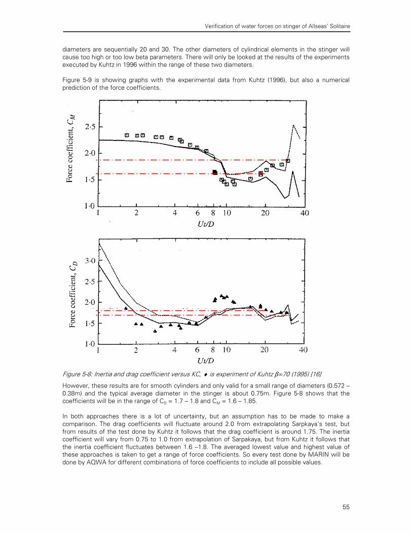
Verification of water forces on stinger of Allseas’ Solitaire
55
diameters are sequentially 20 and 30. The other diameters of cylindrical elements in the stinger will
cause too high or too low beta parameters. There will only be looked at the results of the experiments
executed by Kuhtz in 1996 within the range of these two diameters.
Figure 5-9 is showing graphs with the experimental data from Kuhtz (1996), but also a numerical
prediction of the force coefficients.
Figure 5-8: Inertia and drag coefficient versus KC, ♦ is experiment of Kuhtz β=70 (1995) [16]
However, these results are for smooth cylinders and only valid for a small range of diameters (0.572 —
0.38m) and the typical average diameter in the stinger is about 0.75m. Figure 5-8 shows that the
coefficients will be in the range of CD = 1.7 — 1.8 and CM = 1.6 — 1.85.
In both approaches there is a lot of uncertainty, but an assumption has to be made to make a
comparison. The drag coefficients will fluctuate around 2.0 from extrapolating Sarpkaya’s test, but
from results of the test done by Kuhtz it follows that the drag coefficient is around 1.75. The inertia
coefficient will vary from 0.75 to 1.0 from extrapolation of Sarpakaya, but from Kuhtz it follows that
the inertia coefficient fluctuates between 1.6 —1.8. The averaged lowest value and highest value of
these approaches is taken to get a range of force coefficients. So every test done by MARIN will be
done by AQWA for different combinations of force coefficients to include all possible values.

Verification of water forces on stinger of Allseas’ Solitaire
56
Combination Drag coefficient Inertia coefficient
1 1.9 1.1
2 2.1 1.7
Table 5-6: Ranges of drag and inertia coefficient for input in AQWA
The perfect coefficient will never be obtained, because there is not enough information available to
determine these coefficients. By applying these combinations of ranges of force coefficients the
possible values are included. These ranges are based on results of experiments executed in the range
of Re and KC at which the MARIN tests were done. Obviously a concrete conclusion will not be the
answer in the comparison, but by applying these ranges something can be said about the calculation
method of AQWA for the stinger forces and moments.
5.6.3 Vortex shedding
Extrapolation of the results for the lift coefficient by Sarpkaya for the MARIN conditions will give very
high lift coefficients. This means that the lift force around the elements in the stinger will be higher
due to the MARIN combination of a lower Re number.
Figure 5-9: Lift coefficient versus KC number for various Re numbers
From Figure 5-10 it can be seen that the lift coefficient will be in the order of 1.5 — 4.0. This is much
higher than attained before with a higher Reynolds number.
5.6.4 Interference
The magnitude of interference at the lower Reynolds number will change also. There will be less
interference due to the MARIN conditions, which also follows from Figure 5-11.
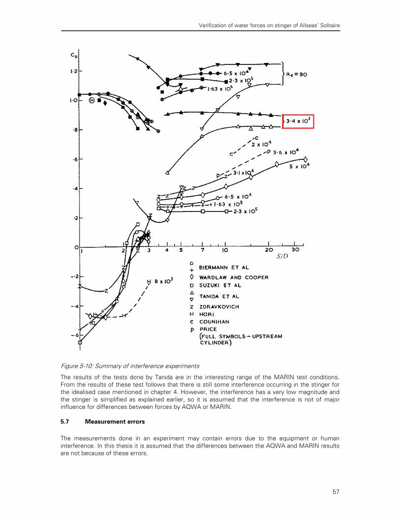
Verification of water forces on stinger of Allseas’ Solitaire
57
Figure 5-10: Summary of interference experiments
The results of the tests done by Tanida are in the interesting range of the MARIN test conditions.
From the results of these test follows that there is still some interference occurring in the stinger for
the idealised case mentioned in chapter 4. However, the interference has a very low magnitude and
the stinger is simplified as explained earlier, so it is assumed that the interference is not of major
influence for differences between forces by AQWA or MARIN.
5.7 Measurement errors
The measurements done in an experiment may contain errors due to the equipment or human
interference. In this thesis it is assumed that the differences between the AQWA and MARIN results
are not because of these errors.

Verification of water forces on stinger of Allseas’ Solitaire
58
Verification of water forces on stinger of Allseas’ Solitaire
59
6 AQWA versus MARIN
6.1 Introduction
In this chapter the main comparison is done for AQWA versus MARIN results for the same conditions
at both models. For the regular waves a comparison is made based on the RAO’s of the ship motions
and stinger forces/moments. For irregular waves the comparison is based on the standard deviations,
RAO’s and Weibull extreme values. To be able to compare the stinger forces and moments, the
motions of the ship are calibrated in AQWA to equal the motions measured in MARIN. When the
same ship motions are obtained a good comparison of the stinger forces and moments can be done.
A statistical analysis, response functions and the extreme values will do the comparison of the forces
and moments. The theory of these analyses is already described in chapter 5. For the statistical
analysis a comparison is made between the standard deviation and RAO, because this value gives the
magnitude of the dynamic forces and moments. The response functions for irregular waves are
gathered out of the AQWA results as is shown in Appendix H.
6.2 AQWA Model
An AQWA model was already available of the Solitaire with his stinger from earlier calculations.
However, the scale model used at MARIN does not coincide exactly with the available AQWA model.
So some changes had to be executed to obtain a fair comparison between AQWA and MARIN. For
the Solitaire this meant a different lay out of the heels at the stern of the vessel en the weight and
moments of radii had to be changed to coincide with the MARIN values (Appendices E and G). The
AQWA model for the test of 2000 needed some extra adaptations. In Appendix I the AQWA models
of the two tests are plotted.
6.3 Ship motions
To make a good comparison between the calculated forces and moment by AQWA against those
measured by MARIN, the ship motions must be the same in AQWA as in MARIN. This way the
differences found can be assigned to the calculated forces done by the Morison equation in AQWA
and the forces due to movement of the ship will be excluded. However, obtaining the exact same
motions in AQWA as in MARIN is a time consuming job and little difference between the ship
motions of AQWA and MARIN is accepted. Besides, sometimes MARIN founded movement, which
are odd, like a sway motion with a regular wave with heading 180°. The ability to change the motions is limited in AQWA, so not in every case a satisfied result can be
obtained. Sometimes AQWA was not able to obtain the values of MARIN. From this moment on, for
every test only the results of the stinger forces and moments will be showed, but at every test the
ship motions were first calibrated. These ship motions can be found in Appendix J for test 1993 and
in Appendix K for test 2000.
It was impossible to calibrate the RAO phases of the ship motions in AQWA. In the comparison of
AQWA versus MARIN the difference in phases between the ship motion was not taken into account.
However, the phase’s differences can have a severe influence on the forces between the two
models.
6.4 MARIN tests 1993 versus AQWA
6.4.1 Current MARIN Tests 1993 versus AQWA
For steady current flow the drag coefficient will be determined from Figure 6-1, which is gathered
from several experiments.
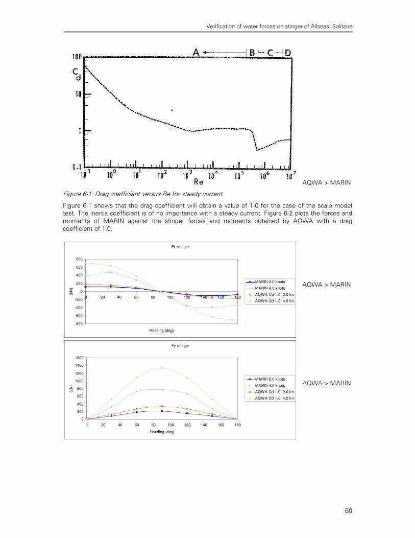
Verification of water forces on stinger of Allseas’ Solitaire
60
Figure 6-1: Drag coefficient versus Re for steady current
Figure 6-1 shows that the drag coefficient will obtain a value of 1.0 for the case of the scale model
test. The inertia coefficient is of no importance with a steady current. Figure 6-2 plots the forces and
moments of MARIN against the stinger forces and moments obtained by AQWA with a drag
coefficient of 1.0.
Fx stinger
-800
-600
-400
-200
0
200
400
600
800
0 20 40 60 80 100 120 140 160 180
Heading (deg)
(kN
)
MARIN 2.0 knots
MARIN 4.0 knots
AQWA Cd 1.0 ;2.0 kn
AQWA Cd 1.0; 4.0 kn
Fy stinger
0
200
400
600
800
1000
1200
1400
1600
0 20 40 60 80 100 120 140 160 180
Heading (deg)
(kN
)
MARIN 2.0 knots
MARIN 4.0 knots
AQWA Cd 1.0; 2.0 kn
AQWA Cd 1.0; 4.0 kn
AQWA > MARIN
AQWA > MARIN
AQWA > MARIN

Verification of water forces on stinger of Allseas’ Solitaire
61
Fz stinger
-350
-300
-250
-200
-150
-100
-50
0
50
100
150
0 20 40 60 80 100 120 140 160 180
Heading (deg)
(kN
)
MARIN 2.0 knots
MARIN 4.0 knots
AQWA Cd 1.0; 2.0 kn
AQWA Cd 1.0; 4.0 kn
Mx stinger
0
5000
10000
15000
20000
25000
30000
0 20 40 60 80 100 120 140 160 180
Heading (deg)
(kN
m)
MARIN 2.0 knots
MARIN 4.0 knots
AQWA Cd 1.0; 2.0 kn
AQWA Cd 1.0; 4.0 kn
My stinger
-40000
-30000
-20000
-10000
0
10000
20000
0 20 40 60 80 100 120 140 160 180
Heading (deg)
(kN
m)
MARIN 2.0 knots
MARIN 4.0 knots
AQWA Cd 1.0; 2.0 kn
AQWA Cd 1.0; 4.0 kn
Mz stinger
-80000
-70000
-60000
-50000
-40000
-30000
-20000
-10000
0
0 20 40 60 80 100 120 140 160 180
Heading (deg)
(kN
m)
MARIN 2.0 knots
MARIN 4.0 knots
AQWA Cd 1.0; 2.0 kn
AQWA Cd 1.0; 4.0 kn
Figure 6-2: Current tests AQWA versus MARIN
AQWA > MARIN
MARIN > AQWA
AQWA > MARIN
MARIN > AQWA

Verification of water forces on stinger of Allseas’ Solitaire
62
AQWA follows the same trend for the forces and moments versus the heading as found in the
MARIN tests. With a drag coefficient of 1.0 the AQWA outputs are higher for every force direction
except for the Fz and the moment around the y-axis. Here the MARIN results are higher, but there is
a small difference. This difference could only be caused by the difference in drag forces between the
two models. The higher magnitude found by AQWA for the other forces could be assigned to the
interference, which in reality will result in a lower drag coefficient then AQWA assumes. Due to these
effects the total drag coefficient should not be 1.0, but lower. However, the lower calculated Fz and
My by AQWA are not in line with this conclusion, what can be assigned to the angle of attack effect.
The Fy force found in the MARIN tests with a current heading of 0° or 180° is 0. This means that vortex shedding, which could result in lift forces, will not cause a force perpendicular to the current.
6.4.2 Regular wave MARIN tests 1993 versus AQWA
The RAO’s of the ship motions were calibrated in AQWA and compared with the RAO ship motions
obtained by MARIN. This way the same motions are present in the two comparable data. The results
of the RAO ship motions comparison can be found in Appendix J. In the figures 6-3, 6-4, 6-5 the
RAO’s of the MARIN and AQWA stinger forces and moment are compared for different headings
Regular waves H = 4.0 m, Heading 180°°°°
Fx Heading 180
0
50
100
150
200
250
300
350
0 0.1 0.2 0.3 0.4 0.5 0.6 0.7 0.8
Frequency (rad/s )
RA
O F
x (
kN
/m)
MARIN
Cd 1.9 Cm 1.1
Cd 2.1 Cm 1.7
Fy Heading 180
0
5
10
15
20
25
30
0 0.1 0.2 0.3 0.4 0.5 0.6 0.7 0.8
Frequency (rad/s )
RA
O F
y (
kN
/m)
MARIN
Cd 1.9 Cm 1.1
Cd 2.1 Cm 1.7
Fz Heading 180
0
100
200
300
400
500
600
700
800
0 0.1 0.2 0.3 0.4 0.5 0.6 0.7 0.8
Frequency (rad/s )
RA
O F
z (
kN
/m)
MARIN
Cd 1.9 Cm 1.1
Cd 2.1 Cm 1.7
Mx Heading 180
0
200
400
600
800
1000
1200
1400
0 0.1 0.2 0.3 0.4 0.5 0.6 0.7 0.8
Frequency (rad/s )
RA
O M
x (
kN
m/m
)
MARIN
Cd 1.9 Cm 1.1
Cd 2.1 Cm 1.7
My Heading 180
0
10000
20000
30000
40000
50000
60000
70000
0 0.1 0.2 0.3 0.4 0.5 0.6 0.7 0.8
Frequency (rad/s )
RA
O M
y (
kN
m/m
)
MARIN
Cd 1.9 Cm 1.1
Cd 2.1 Cm 1.7
Mz Heading 180
0
500
1000
1500
2000
2500
3000
0 0.1 0.2 0.3 0.4 0.5 0.6 0.7 0.8
Frequency (rad/s )
RA
O M
z (
kN
m/m
)
MARIN
Cd 1.9 Cm 1.1
Cd 2.1 Cm 1.7
Figure 6-3: Compilation of regular wave test results AQWA versus MARIN for a 180 degrees heading
For a heading of 180° the ship motions were calibrated as accurate as possible. However, MARIN
found sway, roll and yaw movement, which is odd at a 180 heading. One could imagine that a wave
encountering a ship from 180 degrees would not give the ship a movement perpendicular to this
wave due to the geometry of the ship. AQWA was not able to produce these movements, however
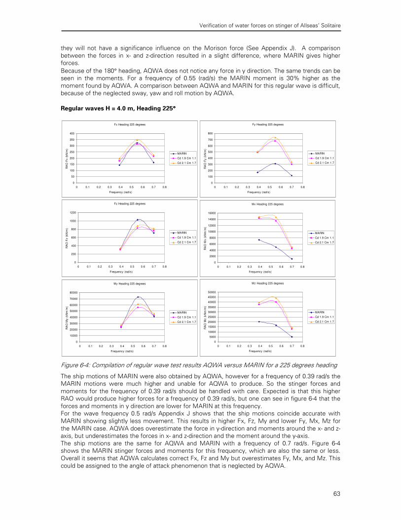
Verification of water forces on stinger of Allseas’ Solitaire
63
they will not have a significance influence on the Morison force (See Appendix J). A comparison
between the forces in x- and z-direction resulted in a slight difference, where MARIN gives higher
forces.
Because of the 180° heading, AQWA does not notice any force in y direction. The same trends can be
seen in the moments. For a frequency of 0.55 (rad/s) the MARIN moment is 30% higher as the
moment found by AQWA. A comparison between AQWA and MARIN for this regular wave is difficult,
because of the neglected sway, yaw and roll motion by AQWA.
Regular waves H = 4.0 m, Heading 225°°°°
Fx Heading 225 degrees
0
50
100
150
200
250
300
350
400
0 0.1 0.2 0.3 0.4 0.5 0.6 0.7 0.8
Frequency (rad/s)
RA
O F
x (
kN
/m)
MARIN
Cd 1.9 Cm 1.1
Cd 2.1 Cm 1.7
Fy Heading 225 degrees
0
100
200
300
400
500
600
700
800
0 0.1 0.2 0.3 0.4 0.5 0.6 0.7 0.8
Frequency (rad/s)
RA
O F
y (
kN
/m)
MARIN
Cd 1.9 Cm 1.1
Cd 2.1 Cm 1.7
Fz Heading 225 degrees
0
200
400
600
800
1000
1200
0 0.1 0.2 0.3 0.4 0.5 0.6 0.7 0.8
Frequency (rad/s)
RA
O F
z (
kN
/m)
MARIN
Cd 1.9 Cm 1.1
Cd 2.1 Cm 1.7
Mx Heading 225 degrees
0
2000
4000
6000
8000
10000
12000
14000
16000
0 0.1 0.2 0.3 0.4 0.5 0.6 0.7 0.8
Frequency (rad/s)
RA
O M
x (
kN
m/m
)
MARIN
Cd 1.9 Cm 1.1
Cd 2.1 Cm 1.7
My Heading 225 degrees
0
10000
20000
30000
40000
50000
60000
70000
80000
0 0.1 0.2 0.3 0.4 0.5 0.6 0.7 0.8
Frequency (rad/s)
RA
O M
y (
kN
m/m
)
MARIN
Cd 1.9 Cm 1.1
Cd 2.1 Cm 1.7
Mz Heading 225 degrees
0
5000
10000
15000
20000
25000
30000
35000
40000
45000
50000
0 0.1 0.2 0.3 0.4 0.5 0.6 0.7 0.8
Frequency (rad/s)
RA
O M
z (
kN
m/m
)
MARIN
Cd 1.9 Cm 1.1
Cd 2.1 Cm 1.7
Figure 6-4: Compilation of regular wave test results AQWA versus MARIN for a 225 degrees heading
The ship motions of MARIN were also obtained by AQWA, however for a frequency of 0.39 rad/s the
MARIN motions were much higher and unable for AQWA to produce. So the stinger forces and
moments for the frequency of 0.39 rad/s should be handled with care. Expected is that this higher
RAO would produce higher forces for a frequency of 0.39 rad/s, but one can see in figure 6-4 that the
forces and moments in y direction are lower for MARIN at this frequency.
For the wave frequency 0.5 rad/s Appendix J shows that the ship motions coincide accurate with
MARIN showing slightly less movement. This results in higher Fx, Fz, My and lower Fy, Mx, Mz for
the MARIN case. AQWA does overestimate the force in y-direction and moments around the x- and z-
axis, but underestimates the forces in x- and z-direction and the moment around the y-axis.
The ship motions are the same for AQWA and MARIN with a frequency of 0.7 rad/s. Figure 6-4
shows the MARIN stinger forces and moments for this frequency, which are also the same or less.
Overall it seems that AQWA calculates correct Fx, Fz and My but overestimates Fy, Mx, and Mz. This
could be assigned to the angle of attack phenomenon that is neglected by AQWA.

Verification of water forces on stinger of Allseas’ Solitaire
64
Regular waves H = 4.0 m, Heading 270°°°°
Fx Heading 270 degrees
0
20
40
60
80
100
120
140
160
180
200
0 0.1 0.2 0.3 0.4 0.5 0.6 0.7 0.8
Frequency (rad/s)
RA
O F
x (
kN
/m)
MARIN
Cd 1.9 Cm 1.1
Cd 2.1 Cm 1.7
Fy Heading 270 degrees
0
50
100
150
200
250
300
350
400
450
0 0.1 0.2 0.3 0.4 0.5 0.6 0.7 0.8
Frequency (rad/s)
RAOFy(kN/m)
MARIN
Cd 1.9 Cm 1.1
Cd 2.1 Cm 1.7
Fz Heading 270 degrees
0
100
200
300
400
500
600
700
800
900
0 0.1 0.2 0.3 0.4 0.5 0.6 0.7 0.8
Frequency (rad/s)
RA
O F
z (
kN
/m)
MARIN
Cd 1.9 Cm 1.1
Cd 2.1 Cm 1.7
Mx Heading 270 degrees
-2000
0
2000
4000
6000
8000
10000
12000
14000
0 0.1 0.2 0.3 0.4 0.5 0.6 0.7 0.8
Frequency (rad/s)R
AO
Mx
(k
Nm
/m)
MARIN
Cd 1.9 Cm 1.1
Cd 2.1 Cm 1.7
My Heading 270 degrees
0
10000
20000
30000
40000
50000
60000
0 0.1 0.2 0.3 0.4 0.5 0.6 0.7 0.8
Frequency (rad/s)
RA
O M
y (
kN
m/m
)
MARIN
Cd 1.9 Cm 1.1
Cd 2.1 Cm 1.7
Mz Heading 270 degrees
-5000
0
5000
10000
15000
20000
25000
30000
35000
0 0.1 0.2 0.3 0.4 0.5 0.6 0.7 0.8
Frequency (rad/s)
RAOMz(kN
MARIN
Cd 1.9 Cm 1.1
Cd 2.1 Cm 1.7
Figure 6-5: Compilation of regular wave test results AQWA versus MARIN for a 270 degrees heading
The RAO ship motions of MARIN showed a surge and yaw motion, which could not be produced by
AQWA. Appendix J shows that in every movement MARIN RAO is much higher than the AQWA RAO
for different frequencies. A logic result would be that the MARIN stinger forces and moments would
be higher than the AQWA result in figure 6-5. However, the MARIN Fy, Mx and Mz are lower at a
frequency of 0.39 rad/s and about the same at a frequency of 0.55 rad/s. The ship motions did not
coincide in this test, so the results of the loads are difficult to compare.
6.4.3 Irregular wave MARIN test 1993 versus AQWA heading 180°
Obtaining the same ship motions as measured in MARIN was a difficult task. MARIN observed sway,
roll and yaw motions with a heading of 180 degrees. AQWA will not produce these motions, but with
taking an irregular wave heading of 183° the ship motions coincide more. This way it was possible to compare the stinger forces and moments. However, for irregular waves it is hard to obtain the same
ship motion which can be seen in Appendix J. The ship motions are not exactly the same, but a
comparison for forces is made that should be handled with care. The stinger forces and moment for
AQWA and MARIN are compared with the standard deviations, response functions and the extreme
values in respectively figures 6-6, 6-7 and 6-8.
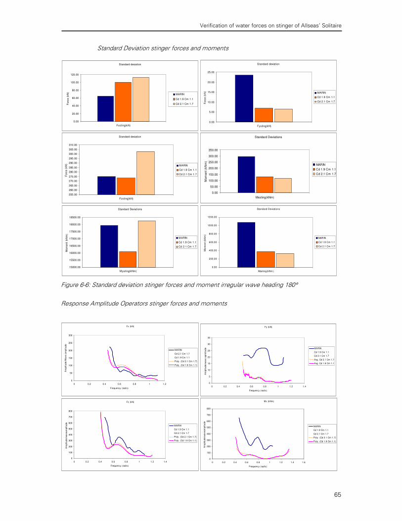
Verification of water forces on stinger of Allseas’ Solitaire
65
Standard Deviation stinger forces and moments
Standard deviation
0.00
20.00
40.00
60.00
80.00
100.00
120.00
Fxsting(kN)
Fo
rce
(k
N)
MARIN
Cd 1.9 Cm 1.1
Cd 2.1 Cm 1.7
Standard deviation
0.00
5.00
10.00
15.00
20.00
25.00
Fysting(kN)
Fo
rce
(k
N)
MARIN
Cd 1.9 Cm 1.1
Cd 2.1 Cm 1.7
Standard deviation
255.00
260.00
265.00
270.00
275.00
280.00
285.00
290.00
295.00
300.00
305.00
310.00
Fzsting(kN)
Fo
rce
(kN
)
MARIN
Cd 1.9 Cm 1.1
Cd 2.1 Cm 1.7
Standard Deviations
0.00
50.00
100.00
150.00
200.00
250.00
300.00
350.00
Mxsting(kNm)
Mo
me
nt
(kN
m)
MARIN
Cd 1.9 Cm 1.1
Cd 2.1 Cm 1.7
Standard Deviations
15000.00
15500.00
16000.00
16500.00
17000.00
17500.00
18000.00
18500.00
Mysting(kNm)
Mo
me
nt
(kN
m)
MARIN
Cd 1.9 Cm 1.1
Cd 2.1 Cm 1.7
Standard Deviations
0.00
200.00
400.00
600.00
800.00
1000.00
1200.00
Mzs ting(kNm )
Mo
me
nt (k
Nm
)
MARIN
Cd 1.9 Cm 1.1
Cd 2.1 Cm 1.7
Figure 6-6: Standard deviation stinger forces and moment irregular wave heading 180°
Response Amplitude Operators stinger forces and moments
Fx (kN)
0
50
100
150
200
250
300
0 0.2 0.4 0.6 0.8 1 1.2
Frequency (rad/s)
Am
plit
ud
e/W
av
e a
mp
litu
de
MARIN
Cd 2.1 Cm 1.7
Cd 1.9 Cm 1.1
Poly. (Cd 2.1 Cm 1.7)
Poly. (Cd 1.9 Cm 1.1)
Fy (kN)
0
5
10
15
20
25
30
35
0 0.2 0.4 0.6 0.8 1 1.2 1.4
Frequency (rad/s)
Am
plit
ud
e/w
ave
ap
mlit
ud
e MARIN
Cd 1.9 Cm 1.1
Cd 2.1 Cm 1.7
Avg. Cd 2.1 Cm 1.7
Avg. Cd 1.9 Cm 1.1
Fz (kN)
0
100
200
300
400
500
600
700
800
0 0.2 0.4 0.6 0.8 1 1.2 1.4
Frequency (rad/s)
Am
plit
ud
e/w
av
ea
mp
litu
de
MARIN
Cd 1.9 Cm 1.1
Cd 2.1 Cm 1.7
Poly. (Cd 2.1 Cm 1.7)
Poly. (Cd 1.9 Cm 1.1)
Mx (kNm)
0
100
200
300
400
500
600
700
800
0 0.2 0.4 0.6 0.8 1 1.2 1.4 1.6
Frequency (rad/s)
Am
plit
ud
e/w
av
ea
mp
litu
de
MARIN
Cd 1.9 Cm 1.1
Cd 2.1 Cm 1.7
Poly. (Cd 2.1 Cm 1.7)
Poly. (Cd 1.9 Cm 1.1)

Verification of water forces on stinger of Allseas’ Solitaire
66
My (kNm)
0
10000
20000
30000
40000
50000
60000
0 0.2 0.4 0.6 0.8 1 1.2
Frequency (rad/s)
Am
plit
ud
e/
Wa
ve
Am
plit
ud
e
MARIN
Cd 1.9 Cm 1.1
Cd 2.1 Cm 1.7
Poly. (Cd 2.1 Cm 1.7)
Poly. (Cd 1.9 Cm 1.1)
Mz (kNm)
0
500
1000
1500
2000
2500
0 0.2 0.4 0.6 0.8 1 1.2 1.4 1.6
Frequency (rad/s)
Am
plit
ud
e/
Wav
e a
mplitu
de
MARIN
Cd 1.9 Cm 1.1
Cd 2.1 Cm 1.7
Poly. (Cd 2.1 Cm 1.7)
Poly. (Cd 1.9 Cm 1.1)
Figure 6-7: RAO's of stinger forces and moment for irregular wave heading 180°
Weibull distribution extreme values 0.1%
Weibull max values 0.1 %Fx
-800
-600
-400
-200
0
200
400
600
Maxcrests Maxtrough
(kN
)
MARIN
Cd 1.9 Cm 1.1
Cd 2.1 Cm 1.7
Weibull m ax values 0.1 % Fy
-150
-100
-50
0
50
100
150
200
Maxcres ts Maxtrough
(kN
)
MARIN
Cd 1.9 Cm 1.1
Cd 2.1 Cm 1.7
W eibull max values 0.1 % Fz
-1500
-1000
-500
0
500
1000
1500
2000
Maxcrests Maxtrough
(kN
)
MARIN
Cd 1.9 Cm 1.1
Cd 2.1 Cm 1.7
Weibull m ax values 0.1 % Mx
-4000
-3000
-2000
-1000
0
1000
2000
3000
Maxcres ts Maxtrough
(kN
m) MARIN
Cd 1.9 Cm 1.1
Cd 2.1 Cm 1.7
Weibull m ax values 0.1 % My
-100000
-80000
-60000
-40000
-20000
0
20000
40000
60000
80000
100000
Maxcres ts Maxtrough(kN
m) MARIN
Cd 1.9 Cm 1.1
Cd 2.1 Cm 1.7
Weibull max values 0.1 % Mz
-8000
-6000
-4000
-2000
0
2000
4000
6000
8000
Maxcrests Maxtrough(kN
m) MARIN
Cd 1.9 Cm 1.1
Cd 2.1 Cm 1.7
Figure 6-8: Weibull distribution 0.1% extreme values of stinger forces and moments AQWA versus
MARIN for irregular wave heading 180°
It must be stated that for a heading of 180 degrees the most important parameters to compare are
Fx, Fz and My. Looking at these two forces and moment, figure 6-7 shows that AQWA is the same
for Fx and underestimates the Fz and My. This underestimation of the loads by AQWA can be
assigned to the lower RAO of AQWA for the ship motions. The extreme values in figure 6-8 shows
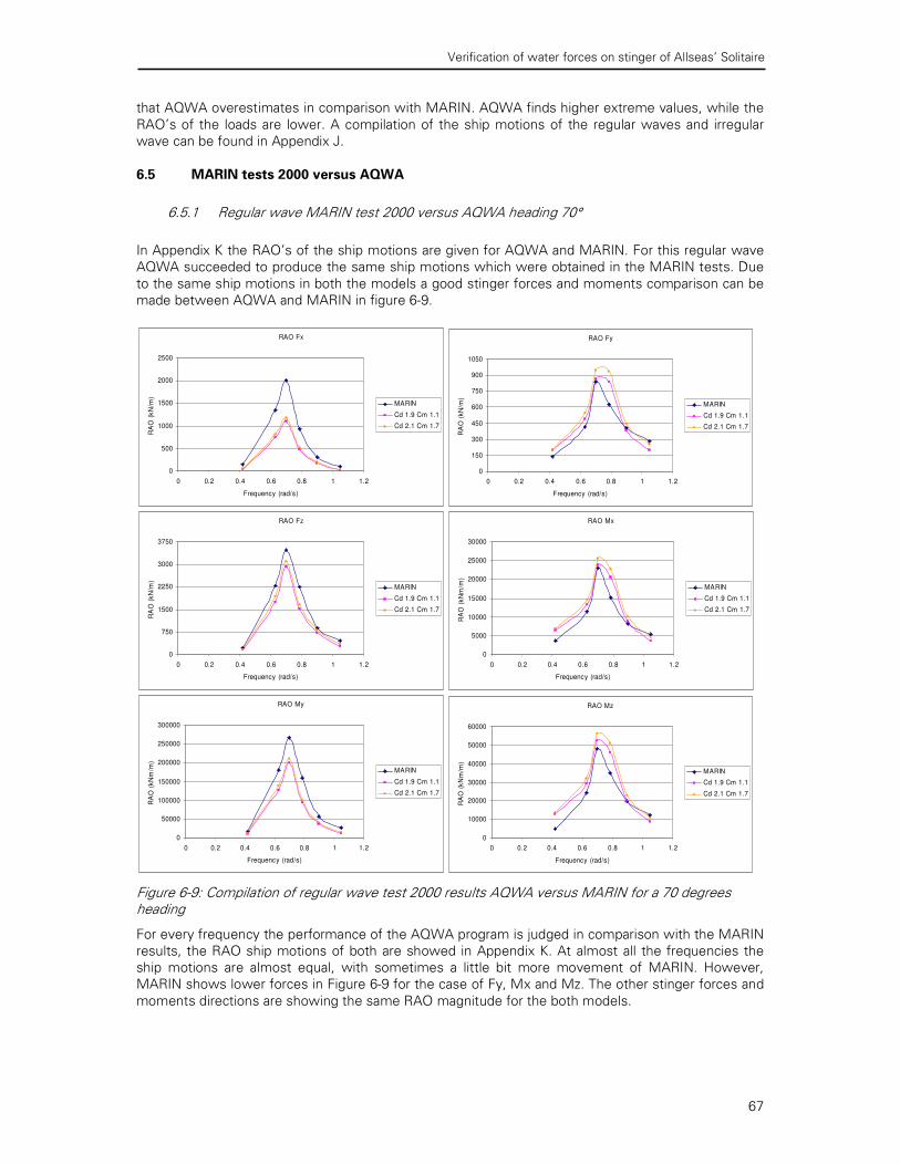
Verification of water forces on stinger of Allseas’ Solitaire
67
that AQWA overestimates in comparison with MARIN. AQWA finds higher extreme values, while the
RAO’s of the loads are lower. A compilation of the ship motions of the regular waves and irregular
wave can be found in Appendix J.
6.5 MARIN tests 2000 versus AQWA
6.5.1 Regular wave MARIN test 2000 versus AQWA heading 70°
In Appendix K the RAO’s of the ship motions are given for AQWA and MARIN. For this regular wave
AQWA succeeded to produce the same ship motions which were obtained in the MARIN tests. Due
to the same ship motions in both the models a good stinger forces and moments comparison can be
made between AQWA and MARIN in figure 6-9.
RAO Fx
0
500
1000
1500
2000
2500
0 0.2 0.4 0.6 0.8 1 1.2
Frequency (rad/s)
RA
O (
kN
/m)
MARIN
Cd 1.9 Cm 1.1
Cd 2.1 Cm 1.7
RAO Fy
0
150
300
450
600
750
900
1050
0 0.2 0.4 0.6 0.8 1 1.2
Frequency (rad/s)
RA
O (
kN
/m)
MARIN
Cd 1.9 Cm 1.1
Cd 2.1 Cm 1.7
RAO Fz
0
750
1500
2250
3000
3750
0 0.2 0.4 0.6 0.8 1 1.2
Frequency (rad/s)
RA
O (
kN
/m)
MARIN
Cd 1.9 Cm 1.1
Cd 2.1 Cm 1.7
RAO Mx
0
5000
10000
15000
20000
25000
30000
0 0.2 0.4 0.6 0.8 1 1.2
Frequency (rad/s)
RA
O (
kN
m/m
)
MARIN
Cd 1.9 Cm 1.1
Cd 2.1 Cm 1.7
RAO My
0
50000
100000
150000
200000
250000
300000
0 0.2 0.4 0.6 0.8 1 1.2
Frequency (rad/s)
RA
O (
kN
m/m
)
MARIN
Cd 1.9 Cm 1.1
Cd 2.1 Cm 1.7
RAO Mz
0
10000
20000
30000
40000
50000
60000
0 0.2 0.4 0.6 0.8 1 1.2
Frequency (rad/s)
RA
O (
kN
m/m
)
MARIN
Cd 1.9 Cm 1.1
Cd 2.1 Cm 1.7
Figure 6-9: Compilation of regular wave test 2000 results AQWA versus MARIN for a 70 degrees heading
For every frequency the performance of the AQWA program is judged in comparison with the MARIN
results, the RAO ship motions of both are showed in Appendix K. At almost all the frequencies the
ship motions are almost equal, with sometimes a little bit more movement of MARIN. However,
MARIN shows lower forces in Figure 6-9 for the case of Fy, Mx and Mz. The other stinger forces and
moments directions are showing the same RAO magnitude for the both models.

Verification of water forces on stinger of Allseas’ Solitaire
68
6.5.2 Irregular wave MARIN test 2000 versus AQWA
Due to limited possibilities to control the ship motions for AQWA in irregular waves, AQWA did not
succeed to reproduce the ship motions of MARIN. Appendix K shows that the standard deviations are
almost similar, but there is a significant difference between the RAO’s of the ship motions. Despite
this difference the stinger forces and moments are compared. The standard deviation, RAO and
extreme value comparison between AQWA and MARIN are shown in respectively the figures 6-10, 6-
11 and 6-12.
Standard Deviations
Standard deviation
0.00
200.00
400.00
600.00
800.00
1000.00
1200.00
Fxsting(kN)
Fo
rce
(k
N)
MARIN
Cd 1.9 Cm 1.1
Cd 2.1 Cm 1.7
Standard deviation
0.00
100.00
200.00
300.00
400.00
500.00
600.00
700.00
800.00
Fysting(kN)
Fo
rce
(k
N)
MARIN
Cd 1.9 Cm 1.1
Cd 2.1 Cm 1.7
Standard deviation
0.00
500.00
1000.00
1500.00
2000.00
2500.00
Fzs ting(kN)
Fo
rce
(kN
)
MARIN
Cd 1.9 Cm 1.1
Cd 2.1 Cm 1.7
Standard Deviations
0.00
2000.00
4000.00
6000.00
8000.00
10000.00
12000.00
14000.00
16000.00
18000.00
Mxsting(kNm)
Mo
me
nt
(kN
m)
MARIN
Cd 1.9 Cm 1.1
Cd 2.1 Cm 1.7
Standard Deviations
0.00
20000.00
40000.00
60000.00
80000.00
100000.00
120000.00
140000.00
160000.00
180000.00
Mysting(kNm)
Mo
me
nt
(kN
m)
MARIN
Cd 1.9 Cm 1.1
Cd 2.1 Cm 1.7
Standard Deviations
0.00
5000.00
10000.00
15000.00
20000.00
25000.00
30000.00
35000.00
40000.00
45000.00
Mzsting(kNm)
Mo
me
nt
(kN
m)
MARIN
Cd 1.9 Cm 1.1
Cd 2.1 Cm 1.7
Figure 6-10: Standard deviations of stinger forces and moments AQWA versus MARIN
Response Amplitude Operator
Fx (kN)
0
200
400
600
800
1000
1200
1400
1600
1800
2000
0 0.2 0.4 0.6 0.8 1 1.2 1.4
Frequency (rad/s)
Am
plit
ud
e/W
av
e a
mp
litu
de
MARIN
Cd 1.9 Cm 1.1
Cd 2.1 Cm 1.7
Poly. (Cd 1.9 Cm 1.1)
Poly. (Cd 2.1 Cm 1.7)
Fy (kN)
0
200
400
600
800
1000
1200
1400
0 0.2 0.4 0.6 0.8 1 1.2 1.4 1.6
Frequency (rad/s)
Am
plit
ud
e/w
av
e a
pm
litu
de
MARIN
Cd 1.9 Cm 1.1
Cd 2.1 Cm 1.7
Poly. (Cd 1.9 Cm 1.1)
Poly. (Cd 2.1 Cm 1.7)

Verification of water forces on stinger of Allseas’ Solitaire
69
Fz (kN)
0
500
1000
1500
2000
2500
3000
3500
4000
0 0.2 0.4 0.6 0.8 1 1.2 1.4
Frequency (rad/s)
Am
plit
ud
e/w
av
ea
mp
litu
de
MARIN
Cd 1.9 Cm 1.1
Cd 2.1 Cm 1.7
Poly. (Cd 1.9 Cm 1.1)
Poly. (Cd 2.1 Cm 1.7)
Mx (kNm)
0
5000
10000
15000
20000
25000
30000
0 0.2 0.4 0.6 0.8 1 1.2 1.4 1.6
Frequency (rad/s)
Am
plit
ud
e/w
av
ea
mp
litu
de
MARIN
Cd 1.9 Cm 1.1
Cd 2.1 Cm 1.7
Poly. (Cd 1.9 Cm 1.1)
Poly. (Cd 2.1 Cm 1.7)
My (kNm)
0
50000
100000
150000
200000
250000
300000
0 0.2 0.4 0.6 0.8 1 1.2 1.4
Frequency (rad/s)
Am
plit
ud
e/
Wa
ve
Am
plit
ud
e
MARIN
Cd 1.9 Cm 1.1
Cd 2.1 Cm 1.7
Poly. (Cd 1.9 Cm 1.1)
Poly. (Cd 2.1 Cm 1.7)
Mz (kNm)
0
10000
20000
30000
40000
50000
60000
70000
80000
0 0.2 0.4 0.6 0.8 1 1.2 1.4 1.6
Frequency (rad/s)
Am
plit
ud
e/
Wa
ve
am
plit
ud
e
MARIN
Cd 1.9 Cm 1.1
Cd 2.1 Cm 1.7
Poly. (Cd 1.9 Cm 1.1)
Poly. (Cd 2.1 Cm 1.7)
Figure 6-11: Response Amplitude Operator of stinger forces and moments AQWA versus MARIN
Weibull distribution 1% extreme values
Weibull m ax values 1 %Fx
-6000
-4000
-2000
0
2000
4000
6000
Maxcrests Maxtroughs
(kN
)
MARIN
Cd 1.9 Cm 1.1
Cd 2.1 Cm 1.7
Weibull m ax values 1 % Fy
-5000
-4000
-3000
-2000
-1000
0
1000
2000
3000
4000
Maxcres ts Maxtroughs
(kN
)
MARIN
Cd 1.9 Cm 1.1
Cd 2.1 Cm 1.7
Weibull max values 1 % Fz
-15000
-10000
-5000
0
5000
10000
Maxcrests Maxtroughs
(kN
)
MARIN
Cd 1.9 Cm 1.1
Cd 2.1 Cm 1.7
Weibull max values 1 % Mx
-150000
-100000
-50000
0
50000
100000
Maxcrests Maxtroughs
(kN
m) MARIN
Cd 1.9 Cm 1.1
Cd 2.1 Cm 1.7
Weibull max values 1 % My
-800000
-600000
-400000
-200000
0
200000
400000
600000
800000
Maxcrests Maxtroughs
(kN
m) MARIN
Cd 1.9 Cm 1.1
Cd 2.1 Cm 1.7
Weibull max values 1 % Mz
-300000
-200000
-100000
0
100000
200000
300000
Maxcrests Maxtroughs
(kN
m) MARIN
Cd 1.9 Cm 1.1
Cd 2.1 Cm 1.7
Figure 6-12: Weibull distribution 1% extreme values of stinger forces and moments AQWA versus MARIN
Again the same trend can be seen in the forces and moments. The Fx, Fz and My are underestimated
by AQWA and the other force and moments are practically the same. There are some differences in
ship motions, because it was impossible to align these motions. However, the extreme values of
AQWA are much higher than found in the MARIN tests. The comparison of the loads in this test is

Verification of water forces on stinger of Allseas’ Solitaire
70
valid, because the ship motions in AQWA were calibrated the same as in the MARIN test. A
compilation of the RAO ship motions for the irregular and regular wave is plotted in Appendix K.
6.6 Influence of force coefficients
The results from earlier paragraphs showed that sometimes AQWA overestimates and sometimes it
underestimates. In chapter 5 the scale effects were determined and a range of force coefficients was
assumed, namely Cd 1.9 Cm 1.1 to Cd 2.1 Cm 1.7. With this range the MARIN tests were verified,
but an interesting issue is to get a view of how much influence these coefficients have on the total
force. Therefore MARIN test 2000 regular wave heading 70° was executed again, but now with also the “extreme” force coefficient combinations of Cd 1.2 Cm 2.0 and Cd 3.5 Cm 1.1. The goal of this
action is to obtain a feeling for the magnitude of influence of these coefficients and this is shown in
figure 6-13.
RAO Fx
0
500
1000
1500
2000
2500
0 0.2 0.4 0.6 0.8 1 1.2
Frequency (rad/s)
RA
O (
kN
/m)
MARIN
Cd 1.2 Cm 2.0
Cd 1.9 Cm 1.1
Cd 2.1 Cm 1.7
Cd 3.5 Cm 1.1
RAO Fy
0
150
300
450
600
750
900
1050
1200
1350
0 0.2 0.4 0.6 0.8 1 1.2
Frequency (rad/s)
RA
O (
kN
/m)
MARIN
Cd 1.2 Cm 2.0
Cd 1.9 Cm 1.1
Cd 2.1 Cm 1.7
Cd 3.5 Cm 1.1
RAO Fz
0
750
1500
2250
3000
3750
4500
5250
0 0.2 0.4 0.6 0.8 1 1.2
Frequency (rad/s)
RA
O (
kN
/m)
MARIN
Cd 1.2 Cm 2.0
Cd 1.9 Cm 1.1
Cd 2.1 Cm 1.7
Cd 3.5 Cm 1.1
RAO Mx
0
5000
10000
15000
20000
25000
30000
35000
0 0.2 0.4 0.6 0.8 1 1.2
Frequency (rad/s)
RA
O (
kN
m/m
) MARIN
Cd 1.2 Cm 2.0
Cd 1.9 Cm 1.1
Cd 2.1 Cm 1.7
Cd 3.5 Cm 1.1
RAO My
0
50000
100000
150000
200000
250000
300000
350000
0 0.2 0.4 0.6 0.8 1 1.2
Frequency (rad/s)
RA
O (
kN
m/m
) MARIN
Cd 1.2 Cm 2.0
Cd 1.9 Cm 1.1
Cd 2.1 Cm 1.7
Cd 3.5 Cm 1.1
RAO Mz
0
10000
20000
30000
40000
50000
60000
70000
80000
0 0.2 0.4 0.6 0.8 1 1.2
Frequency (rad/s)
RA
O (
kN
m/m
) MARIN
Cd 1.2 Cm 2.0
Cd 1.9 Cm 1.1
Cd 2.1 Cm 1.7
Cd 3.5 Cm 1.1
Figure 6-13: Influence of force coefficients on total force due to "extreme" force coefficient combinations
Figure 6-13 shows that for some cases the Cd 3.5 Cm 1.1 combination is a good approximation.
However this combination has never been obtained in an experiment before, so a drag coefficient of
3.5 is impossible for this Re and KC numbers. These figures do show that the force coefficients will
have an influence on the total stinger forces and moments, but these coefficients will have to change
a lot in magnitude to change the loads significant.

Verification of water forces on stinger of Allseas’ Solitaire
71
6.7 Conclusion
To obtain the same standard deviations and ship motions RAO’s for AQWA as observed in the
MARIN tests an iterative process was used. This process consisted of changing the damping in
AQWA to control the ship motions to the wanted MARIN values. However, the ability to control the
motions with this adjusted damping is limited. Especially for irregular waves it is very difficult to
obtain exactly the same RAO’s as in MARIN. With some exceptions, the regular waves ship motions
are well controllable. For irregular waves however, it should be noted that the comparison with these
conditions between AQWA and MARIN should be handled with care.
The current comparison shows that AQWA underestimates the force in the z- direction and
consequently the moment around the y-axis. The other forces and moments are overestimated by
AQWA, which can be assigned to the neglecting effects of interference, angle of attack and free
stream turbulence by AQWA. The difference in forces can only be assigned to the difference in drag
forces, because inertia forces do not play a role in a current condition.
The regular wave comparison shows that AQWA overestimates the force in y direction and the
moments around the x- and z-axis. The forces in x- and z- direction and the moment around the y —
axis are underestimated by AQWA. The underestimation for the force in z direction and the moment
around the y-axis was also observed in the current comparison, so it could be stated that the drag
force causes this difference. However, at the current tests the force in x direction was overestimated.
So AQWA overestimates the drag forces in this direction, but underestimated the total force in x
direction. This could be due to scale effects, but also due to higher inertia forces calculated by
AQWA.
From this whole comparison it followed that not only the choice of the force coefficients is important,
but that the motions of the ship are also very important.
UUDCaDCtF Dm ⋅⋅⋅+⋅⋅⋅= ρρπ
2
1
4)(
2 (Eq 6-1)
In the drag term of the Morison formula stated here, the velocity component is square, while the drag
coefficient is linear. So an increase of the drag coefficient will have less influence than an increase of
the velocity component. The results from paragraphs 6.4 — 6.6 shows that an increase of the drag
coefficient will increase the drag force, but that a small difference between the ship motions of
AQWA and MARIN will cause high difference between the loads. The fact that the drag coefficient is
not the most important factor should be kept in mind. When the ship motions are calibrated correctly
the forces and moments results of AQWA are within the 15% compared with MARIN.

Verification of water forces on stinger of Allseas’ Solitaire
72

Verification of water forces on stinger of Allseas’ Solitaire
73
7 Conclusions and recommendations
7.1 Introduction
The main goal of this thesis is the verification of the accuracy of the program AQWA. The conclusions
for this objective are divided in two sections. The first section concerns the effects that AQWA
neglects. Conclusion can be drawn about what the magnitudes of these neglected effects are.
The second section is the main comparison between the results of the MARIN scale model test and
the AQWA program to show how accurate AQWA calculates. Finally some recommendations are
given.
7.2 Conclusion on neglected effects of AQWA
• Of all the effects investigated only interference of the cylindrical elements, vortex shedding
phenomenon, free stream turbulence and the angle of attack effect can cause differences
between AQWA and reality. The effects of turbulence, sea waves — orbital motion and free ends
are of no influence on the stinger force comparison between AQWA and MARIN.
• Interference is calculated with a simplified stinger to get a view on what the magnitude of
interference could be. It shows that the drag coefficient for the second cylinder in a tandem
arrangement could reduce to 0.21 — 0.5. However, the stinger was reduced to a very simple
construction and the real flow around the cylindrical elements in the stinger is too complex to
consider in this thesis.
• In reality vortex shedding occurs and causes a lift force on the cylindrical element. AQWA does
not take into account this phenomenon. Although this force is not as high as the in line forces, it
can cause oscillations or vibrations of the structure. These vibrations can get severe when the
frequency approaches the natural period of the structure.
• Free stream turbulence can have a severe influence on the force coefficients. In the case of the
Reynolds number, which applies for the stinger, the drag coefficient will increase.
• AQWA works with the independence principle, which states that the force on a oblique cylinder is
calculated by taking the perpendicular velocity component and the “normal” in line drag
coefficient. However, some experiments showed that the drag coefficient should not be taken
“normal” but should differ significantly with the angle of attack. Neglecting this effect can have a
severe effect on the total force on the stinger, because almost all the cylindrical elements have an
angle with the flow.
7.3 Conclusions on comparison AQWA versus MARIN
• A comparison between the scale model test and AQWA is very difficult, because the scale
effects play an important role. Due to these scale effects the Reynolds number is lower at the
scale model test, which complicates the determination of the force coefficients. Estimation of
these coefficients is done based on extrapolation and an experiment by Kuhtz.
• The main comparison in chapter 6 shows that in most cases AQWA overestimates the Fy, Mx
and Mz and underestimates the Fx, Fz and My. Also, it can be stated that the Fx,Fy and My
forces are the most important forces of all and are of most influence on the stinger.
• The magnitude of the drag coefficient determines the total force, but a correct representation of
the velocity is also of high priority. In the Morsion formula the velocity squares, so a little increase

Verification of water forces on stinger of Allseas’ Solitaire
74
in velocity will cause a high increase in the total force. The drag coefficient is linear in this
formula, so an increase will have less influence.
• Despite AQWA’s simplifications and the estimated scale effects, the calculated forces by AQWA
were mostly within 15% of the results of the MARIN test. This conclusion is only valid when the
ship motions of the two models coincide. The Morison force approach used in AQWA can be
seen as a good first estimate of the forces on the stinger.
7.4 Recommendations
• A better understanding of the magnitude of interference, vortex shedding and angle of attack is
needed for the stinger. It is showed in this thesis through simplifications that these effects can
have a severe influence on the force coefficients.
• A tool has to be designed in AQWA to enforce a wanted RAO to the vessel and stinger. AQWA
has the ability to give a certain structure a wanted RAO, but this function will not work for
multiple structures attached to each other. Also more insight is needed in the calculation method
of AQWA.
• Next time a scale model test is used, it should be noted that it is possible to measure the stinger
forces, but due to scale effects they should be handled with care. Due to scale effects the force
coefficients are hard to determine and they have to be estimated based on limited data. More
research is needed concerning the magnitude of the force coefficient for Reynolds and Keulegan
numbers at scale conditions
• For a better verification of the AQWA program a test in reality is needed. Measuring the forces on
the Solitaire stinger at different sea conditions in real life will give an overview of the true forces
on the stinger. This data can be compared with AQWA runs and an accurate verification of the
program can be made. The force coefficients are then known for these conditions and no
uncertainties due to scale effects are in the comparison. A suggested test set-up is made in
Appendix L.

Verification of water forces on stinger of Allseas’ Solitaire
75
References
[1] Introduction to Pipelaying, (revision D Ferbuary 2004), Allseas Engineering bv, Delft, The Netherlands
[2] Technical Specifications D.P Pipelay Vessel Solitaire, (Revision W April 2005), Allseas Engineering
bv, Delft, Netherlands. [3] 011601 - Elongated Solitaire Stinger - Basis of Design, (Document no. 011601-ESS002 Rev. E,
August 2004), Allseas Engineering bv, Delft, Netherlands [4] Engineering Fluid Mechanics, (Eighth Edition, 2005), Clayton T. Crowe/ Donald F. Elger/ John A
Roberson
[5] Hydrodynamics around cylindrical structures, (1st edition, 1997), B. Mutlu Sumer, J∅rgen
Freds∅e, Advanced Series on Ocean Engineering — Volume 12. [6] Offshore Hydrodynamics, (1st Edition, January 2001), J.M.J. Journeé and W.W. Massie, Delft
University of Technology. [7] AQWA Manuals, Century Dynamics Limited.
[8] Stinger Load verification report, (June 2004) IHC Gusto Engineering B.V.
[9] Environmental conditions and environmental loads, Classification Notes No. 30.5, (March 2000), Det Norske Veritas.
[10] Mechanics of Wave force on Offshore Structures (1981), Turgut Sarpkaya and Michael Isaacson. [11] Flow around circular cylinders, Volume 1, (1997), M.M. Zdravkovich. [12] Flow around circular cylinders, Volume 2: Applications, (2003), M.M. Zdravkovich [13] MARIN, Maritime Research Institute Netherlands, Report No. 2.11861-1-GT/DT, Model test on
the pipelay vessel “Solitaire”, (May 1993), Reported by Ir. B. Buchner and H.W. Roelofs. [14] MARIN, Maritime Research Institute Netherlands, Report No. 15946-1-GT, Model test on the
pipelay vessel “Solitaire”, (April 2000), Reported by Ir. R.J. van der Wal and H.W. Roelofs. [15] A new time-domain drag description and its influence on the dynamic behaviour of a cantilever
pipe conveying fluid, (2006), G.L. Kuiper_, A.V. Metrikine, J.A. Battjes, Journal of Fluids and Structures 23 (2007) 429—445.
[16] A numerical study of oscillatory flow about a circular cylinder for low values of beta parameter,
(1996), X.W. Lin, P.W. Bearman and J.M.R. Graham, Journal of Fluids and Structures (1996) 10.

Verification of water forces on stinger of Allseas’ Solitaire
76

Verification of water forces on stinger of Allseas’ Solitaire
77
Appendix A: Personal Data
Institution
Delft University of Technology
Faculty of Fluid Mechanics
Stevinweg 1
2628 CN Delft
Company
Allseas Engineering bv
Innovations Department
Poortweg 12
2612 PA Delft
Student
G.D. Marbus
Oude Delft 96a
2611 CE Delft
06-41278903
Committee
Delft University of Technology, Faculty of Hydraulic Engineering:
Prof.dr.ir. G.S. Stelling
+31-152785426
Dr.ir. W.S.J. Uijttewaal
+31-152781371
Ir. R.J. Labeur
+31-152785069
Delft University of Technology, Faculty Ship Hydrodynamics and Structures:
Prof.dr.ir. R.H.M. Huijsmans
+31-152783598
Allseas Engineering bv:
Ir. J. Marijn Dijk
+31-152681800

Verification of water forces on stinger of Allseas’ Solitaire
78
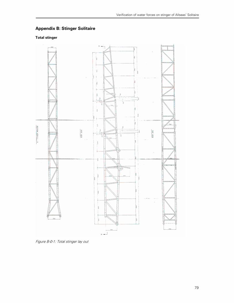
Verification of water forces on stinger of Allseas’ Solitaire
79
Appendix B: Stinger Solitaire
Total stinger
Figure B-0-1: Total stinger lay out

Verification of water forces on stinger of Allseas’ Solitaire
80
Section 1
Figure B-0-2: Old Stinger lay out section 1
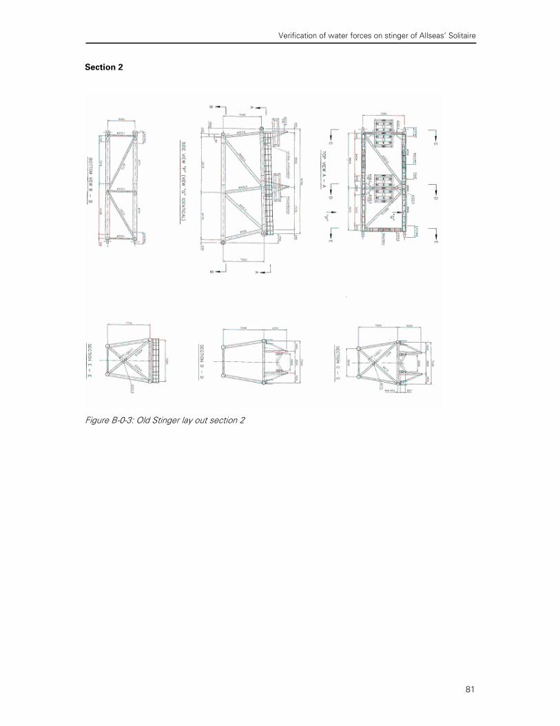
Verification of water forces on stinger of Allseas’ Solitaire
81
Section 2
Figure B-0-3: Old Stinger lay out section 2

Verification of water forces on stinger of Allseas’ Solitaire
82
Section 3
Figure B-4: Old Stinger lay out section 2

Verification of water forces on stinger of Allseas’ Solitaire
83
Appendix C: AQWA information
- AQWA-LINE
Calculation of wave loading from diffraction and radiation around an arbitrarily shaped floating body AQWA-LINE performs a 3-dimensional diffraction/radiation analysis of wave action around a single
floating body, using the classical ‘Green’s function’ approach. A finite element mesh describes the
body surface, and a pulsating ‘source’ is located on each plate element. The combinations of source
strengths required to diffract an incoming regular wave of given period, and to allow body oscillation
in each degree of freedom, are then calculated. From these are obtained the diffraction force, added
mass and radiation damping on the vessel, which are then stored in the AQWA suite database for use
by other AQWA programs. In addition, AQWA-LINE combines them with the body’s motions in all six
degrees of freedom and the associated steady wave drift forces. The program has comprehensive
‘restart’ facilities, to allow the results to be recalculated for different mechanical mass, viscous
damping or mooring stiffness, or for a different length scale factor, without having to repeat the basic
Green’s function analysis. AQWA-LINE is also able to take account of hydrodynamic interaction
between a floating structure and an adjacent fixed structure. AQWA line is used to describe the
motions of the vessel as a result of the motions of the water.
- AQWA-LIBRIUM
Calculation of the equilibrium position of an assembly of floating structures linked by mooring lines or articulations, and calculations of the equilibrium stability AQWA-LIBRIUM takes from AQWA-LINE the wave drift force coefficient on each floating body in
assembly, for each of a series of regular wave periods, and calculates the steady drift forces in an
irregular wave train of any given spectrum. Wind and current loads from any direction are included,
and all loading calculations take account of the changing headings of the various floating bodies.
These steady environmental loads are compared with the loads from articulations and mooring
lines between the bodies, and the position of equilibrium of the assembly found. In addition, a full
finite element description of the body surfaces, extending above the still waterline, is used by
AQWALIBRIUM to compute the buoyancy forces at any position of the bodies. These forces,
together with the structural weight, are also incorporated, so that the final equilibrium is achieved in
all six degrees of freedom of each body in the assembly. No assumption is made that the equilibrium
needs to be a stable one; the final stage in the calculation is to compute the stability derivatives of the
equilibrium.
Since they cover all six degrees of freedom of each body, these derivatives describe stability against
‘fishtailing’ in the horizontal plane, as well as against capsize. AQWA-LIBRIUM can be instructed to
perform calculations for a number of specified wave spectra in turn, producing output in tabular form.
- AQWA — NAUT
Time domain program for wave frequency structure motion and mooring tension analysis in regular waves. AQWA-NAUT for a series of time steps it calculates the total force on the structure, the acceleration,
find the new position of the structure and repeats this. The differences between AQWA DRIFT and
NAUT is that AQWA NAUT calculates with irregular AND regular waves, non-linear hydrostatics and
Froude-Krylov force, 2nd order incident wave and omits drift forces.

Verification of water forces on stinger of Allseas’ Solitaire
84
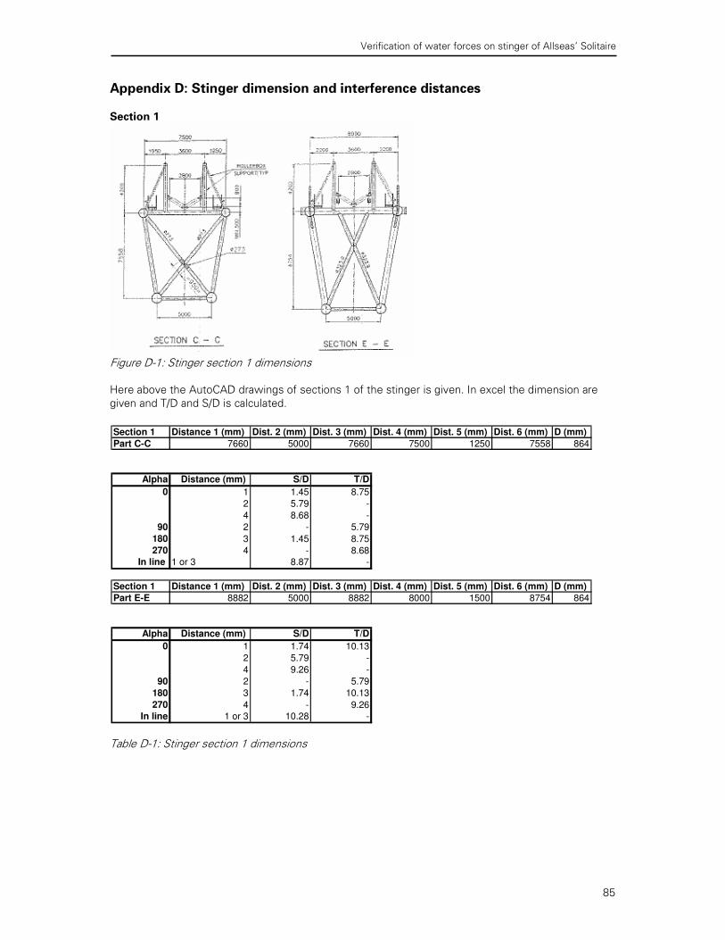
Verification of water forces on stinger of Allseas’ Solitaire
85
Appendix D: Stinger dimension and interference distances
Section 1
Figure D-1: Stinger section 1 dimensions Here above the AutoCAD drawings of sections 1 of the stinger is given. In excel the dimension are
given and T/D and S/D is calculated.
Table D-1: Stinger section 1 dimensions
Section 1 Distance 1 (mm) Dist. 2 (mm) Dist. 3 (mm) Dist. 4 (mm) Dist. 5 (mm) Dist. 6 (mm) D (mm)
Part C-C 7660 5000 7660 7500 1250 7558 864
Alpha Distance (mm) S/D T/D
0 1 1.45 8.75
2 5.79 -
4 8.68 -
90 2 - 5.79
180 3 1.45 8.75
270 4 - 8.68
In line 1 or 3 8.87 -
Section 1 Distance 1 (mm) Dist. 2 (mm) Dist. 3 (mm) Dist. 4 (mm) Dist. 5 (mm) Dist. 6 (mm) D (mm)
Part E-E 8882 5000 8882 8000 1500 8754 864
Alpha Distance (mm) S/D T/D
0 1 1.74 10.13
2 5.79 -
4 9.26 -
90 2 - 5.79
180 3 1.74 10.13
270 4 - 9.26
In line 1 or 3 10.28 -
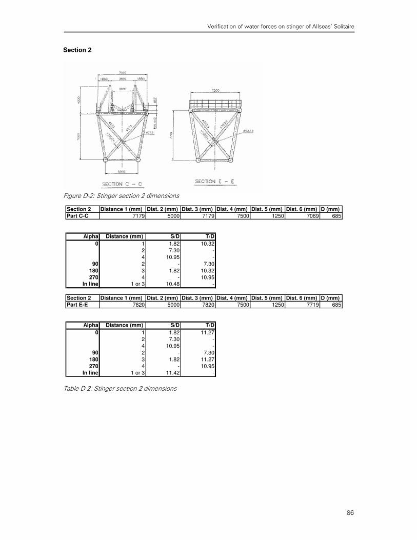
Verification of water forces on stinger of Allseas’ Solitaire
86
Section 2
Figure D-2: Stinger section 2 dimensions
Table D-2: Stinger section 2 dimensions
Section 2 Distance 1 (mm) Dist. 2 (mm) Dist. 3 (mm) Dist. 4 (mm) Dist. 5 (mm) Dist. 6 (mm) D (mm)
Part C-C 7179 5000 7179 7500 1250 7069 685
Alpha Distance (mm) S/D T/D
0 1 1.82 10.32
2 7.30 -
4 10.95 -
90 2 - 7.30
180 3 1.82 10.32
270 4 - 10.95
In line 1 or 3 10.48 -
Section 2 Distance 1 (mm) Dist. 2 (mm) Dist. 3 (mm) Dist. 4 (mm) Dist. 5 (mm) Dist. 6 (mm) D (mm)
Part E-E 7820 5000 7820 7500 1250 7719 685
Alpha Distance (mm) S/D T/D
0 1 1.82 11.27
2 7.30 -
4 10.95 -
90 2 - 7.30
180 3 1.82 11.27
270 4 - 10.95
In line 1 or 3 11.42 -
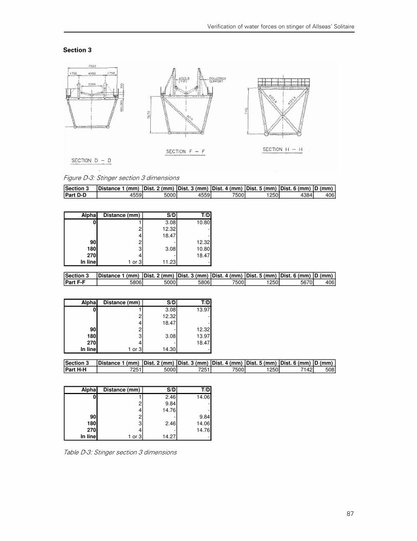
Verification of water forces on stinger of Allseas’ Solitaire
87
Section 3
Figure D-3: Stinger section 3 dimensions
Table D-3: Stinger section 3 dimensions
Section 3 Distance 1 (mm) Dist. 2 (mm) Dist. 3 (mm) Dist. 4 (mm) Dist. 5 (mm) Dist. 6 (mm) D (mm)
Part D-D 4559 5000 4559 7500 1250 4384 406
Alpha Distance (mm) S/D T/D
0 1 3.08 10.80
2 12.32 -
4 18.47 -
90 2 - 12.32
180 3 3.08 10.80
270 4 - 18.47
In line 1 or 3 11.23 -
Section 3 Distance 1 (mm) Dist. 2 (mm) Dist. 3 (mm) Dist. 4 (mm) Dist. 5 (mm) Dist. 6 (mm) D (mm)
Part F-F 5806 5000 5806 7500 1250 5670 406
Alpha Distance (mm) S/D T/D
0 1 3.08 13.97
2 12.32 -
4 18.47 -
90 2 - 12.32
180 3 3.08 13.97
270 4 - 18.47
In line 1 or 3 14.30 -
Section 3 Distance 1 (mm) Dist. 2 (mm) Dist. 3 (mm) Dist. 4 (mm) Dist. 5 (mm) Dist. 6 (mm) D (mm)
Part H-H 7251 5000 7251 7500 1250 7142 508
Alpha Distance (mm) S/D T/D
0 1 2.46 14.06
2 9.84 -
4 14.76 -
90 2 - 9.84
180 3 2.46 14.06
270 4 - 14.76In line 1 or 3 14.27 -

Verification of water forces on stinger of Allseas’ Solitaire
88

Verification of water forces on stinger of Allseas’ Solitaire
89
Appendix E: MARIN scale model dimensions test 1993
Table E-1: MARIN scale model dimension test 1993

Verification of water forces on stinger of Allseas’ Solitaire
90
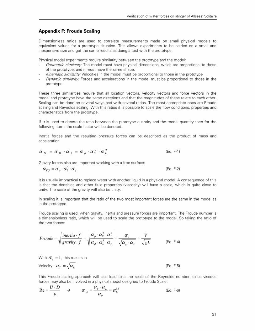
Verification of water forces on stinger of Allseas’ Solitaire
91
Appendix F: Froude Scaling
Dimensionless ratios are used to correlate measurements made on small physical models to
equivalent values for a prototype situation. This allows experiments to be carried on a small and
inexpensive size and get the same results as doing a test with the prototype.
Physical model experiments require similarity between the prototype and the model:
- Geometric similarity: The model must have physical dimensions, which are proportional to those of the prototype, and it must have the same shape.
- Kinematic similarity: Velocities in the model must be proportional to those in the prototype - Dynamic similarity: Forces and accelerations in the model must be proportional to those in the
prototype.
These three similarities require that all location vectors, velocity vectors and force vectors in the
model and prototype have the same directions and that the magnitudes of these relate to each other.
Scaling can be done on several ways and with several ratios. The most appropriate ones are Froude
scaling and Reynolds scaling. With this ratios it is possible to scale the flow conditions, properties and
characteristics from the prototype.
If α is used to denote the ratio between the prototype quantity and the model quantity then for the
following items the scale factor will be denoted.
Inertia forces and the resulting pressure forces can be described as the product of mass and
acceleration:
22
LVAMFI αααααα ρ ⋅⋅=⋅= (Eq. F-1)
Gravity forces also are important working with a free surface:
gLFG αααα ρ ⋅⋅= 3 (Eq. F-2)
It is usually impractical to replace water with another liquid in a physical model. A consequence of this
is that the densities and other fluid properties (viscosity) will have a scale, which is quite close to
unity. The scale of the gravity will also be unity.
In scaling it is important that the ratio of the two most important forces are the same in the model as
in the prototype.
Froude scaling is used, when gravity, inertia and pressure forces are important. The Froude number is
a dimensionless ratio, which will be used to scale the prototype to the model. So taking the ratio of
the two forces:
gL
V
fgravity
finertiaFroude
Lg
V
gL
LV=
⋅=
⋅⋅
⋅⋅=
⋅
⋅=
αα
α
ααα
ααα
ρ
ρ
3
22
(Eq. F-4)
With 1=gα , this results in
Velocity - LT αα = (Eq. F-5)
This Froude scaling approach will also lead to a the scale of the Reynolds number, since viscous
forces may also be involved in a physical model designed to Froude Scale.
υ
DU ⋅=Re �
5.1
Re L
LV αα
ααα
υ
=⋅
= (Eq. F-6)

Verification of water forces on stinger of Allseas’ Solitaire
92
Another number of importance for this investigation is the Keulegan-Carpenter number, which also
can be scaled:
D
TUKC
⋅= � 1=
⋅=
L
TV
KCα
ααα (Eq. F-7)
So this concludes that KC is not changed when Froude scaling is used.

Verification of water forces on stinger of Allseas’ Solitaire
93
Appendix G: MARIN scale model dimensions test 2000
Table G-1: MARIN scale model dimensions test 2000

Verification of water forces on stinger of Allseas’ Solitaire
94
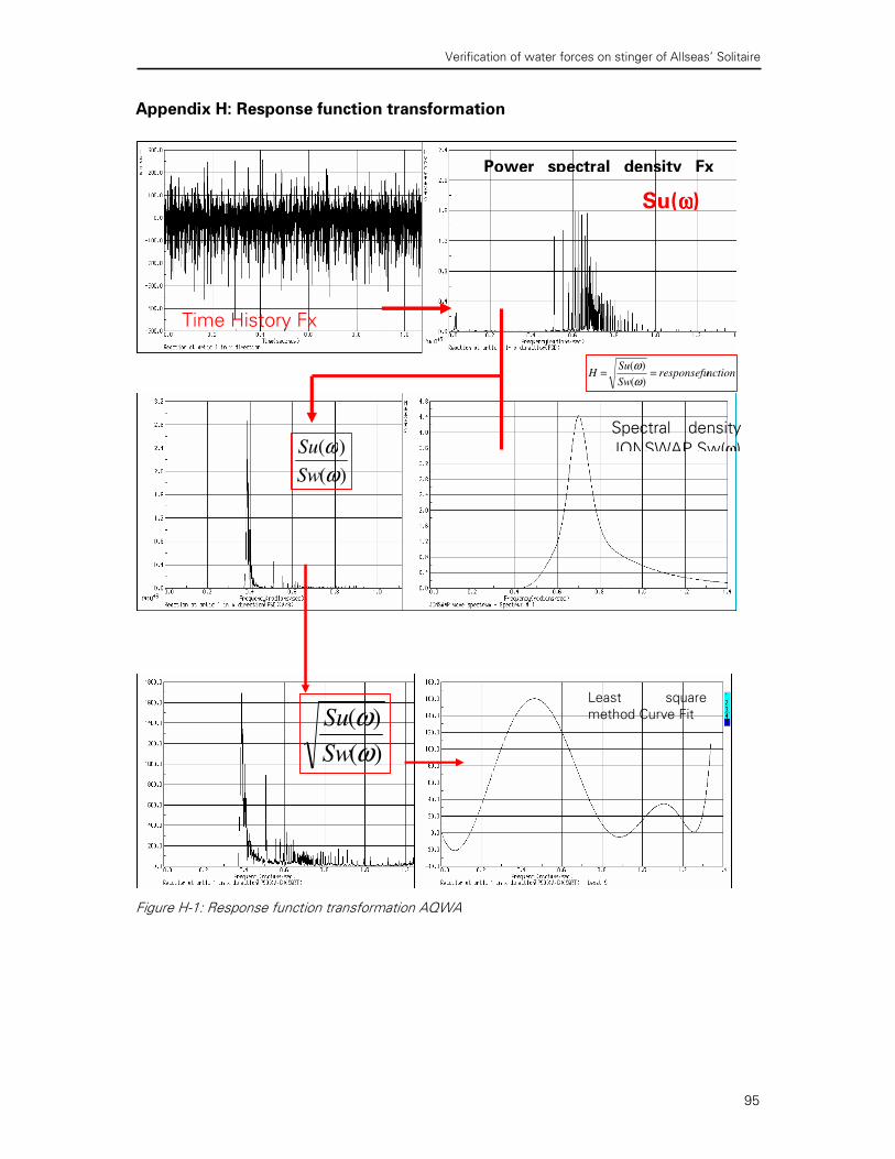
Verification of water forces on stinger of Allseas’ Solitaire
95
Appendix H: Response function transformation
Figure H-1: Response function transformation AQWA
Time History Fx
stinger
Power spectral density Fx
nctionresponsefuSw
SuH ==
)(
)(
ω
ω
Su(ωωωω)
Spectral density
JONSWAP Sw(ω)
)(
)(
ω
ω
Sw
Su
)(
)(
ω
ω
Sw
SuLeast square
method Curve Fit

Verification of water forces on stinger of Allseas’ Solitaire
96
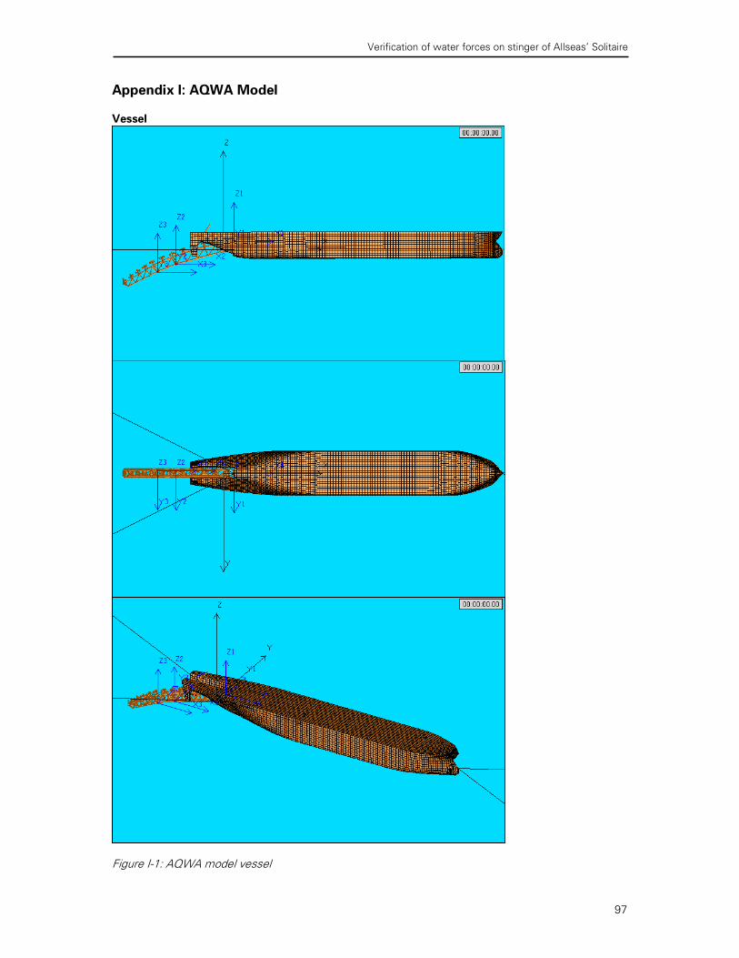
Verification of water forces on stinger of Allseas’ Solitaire
97
Appendix I: AQWA Model
Vessel
Figure I-1: AQWA model vessel
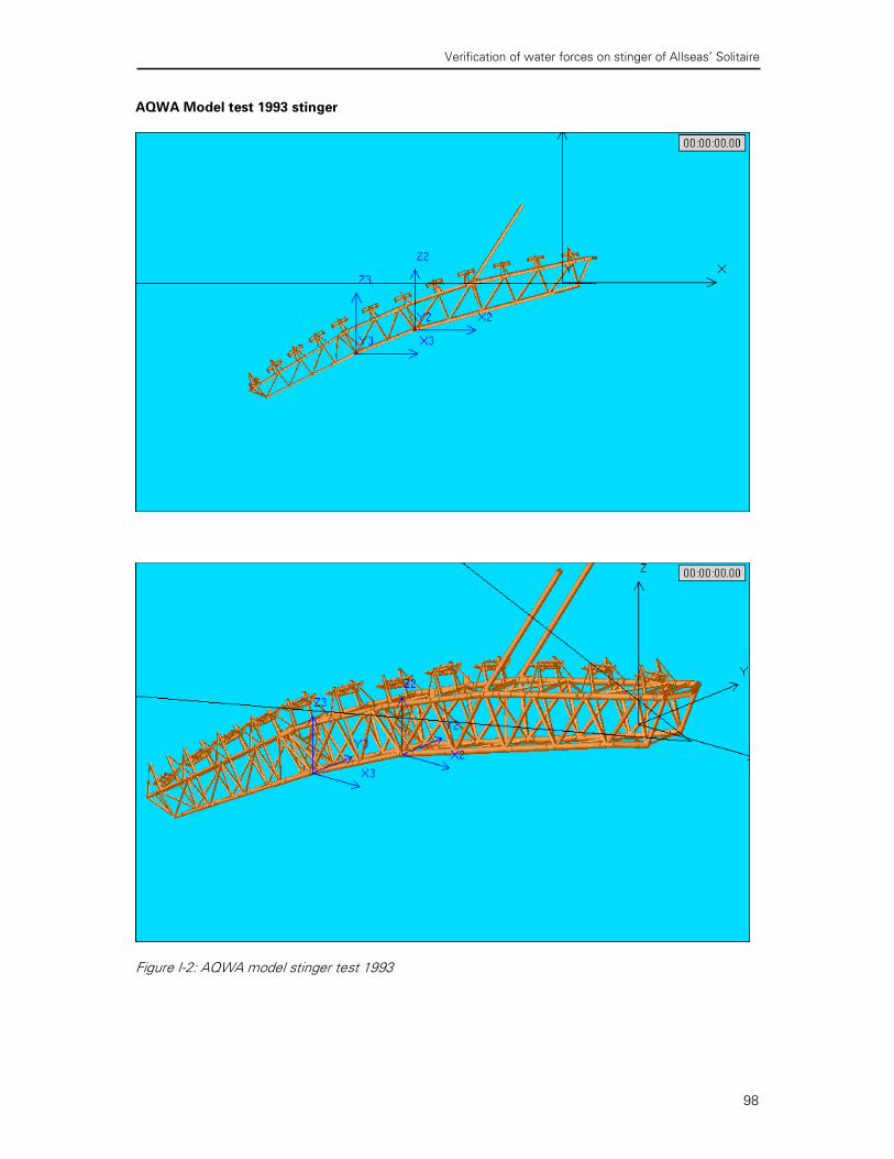
Verification of water forces on stinger of Allseas’ Solitaire
98
AQWA Model test 1993 stinger
Figure I-2: AQWA model stinger test 1993

Verification of water forces on stinger of Allseas’ Solitaire
99
AQWA Model test 2000 Stinger
Figure I-3: AQWA model stinger test 2000

Verification of water forces on stinger of Allseas’ Solitaire
100

Verification of water forces on stinger of Allseas’ Solitaire
101
Appendix J: RAO ship motions test 1993
Irregular 180°°°°
Standard Deviations ship motions
0.00
0.50
1.00
1.50
2.00
2.50
Surge (m) Sway (m ) Heave (m )
Me
tre
s MARIN
Cd 1.9 Cm 1.1
Cd 2.1 Cm 1.7
0.00
0.05
0.10
0.15
0.20
0.25
0.30
0.35
Roll (deg) Pitch (deg) Yaw (deg)
De
gre
es MARIN
Cd 1.9 Cm 1.1
Cd 2.1 Cm 1.7
Figure J-1: Standard deviation of ship motions irregular wave heading 180° test 1993
RAO ship motions
RAO Surge
0
0.05
0.1
0.15
0.2
0.25
0.3
0 0.2 0.4 0.6 0.8 1 1.2 1.4
Frequency (rad/s)
RA
O (
m/m
)
MARIN
Cd 1.9 Cm 1.1
AQWA Vessel
Cd 2.1 Cm 1.7
Poly. (Cd 1.9 Cm 1.1)
Poly. (Cd 2.1 Cm 1.7)
RAO sway
0
0.005
0.01
0.015
0.02
0.025
0.03
0.035
0.04
0 0.2 0.4 0.6 0.8 1 1.2 1.4
Frequency (rad/s)
RA
O (
m/m
)
MARIN
AQWA Vessel
Cd 1.9 Cm 1.1
Cd 2.1 Cm 1.7
Avg. Cd 1.9 Cm 1.1
Avg. Cd 2.1 Cm 1.7
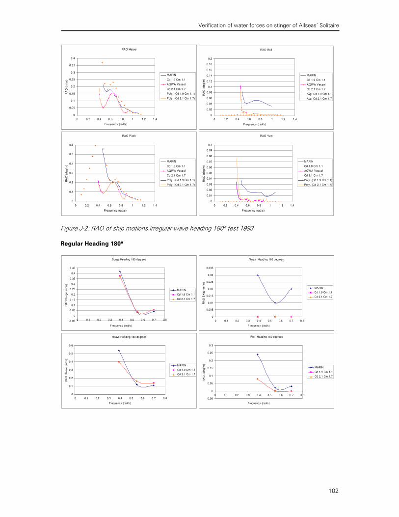
Verification of water forces on stinger of Allseas’ Solitaire
102
RAO Heave
0
0.05
0.1
0.15
0.2
0.25
0.3
0.35
0.4
0 0.2 0.4 0.6 0.8 1 1.2 1.4
Frequency (rad/s)
RA
O (
m/m
)
MARIN
Cd 1.9 Cm 1.1
AQWA Vessel
Cd 2.1 Cm 1.7
Poly. (Cd 1.9 Cm 1.1)
Poly. (Cd 2.1 Cm 1.7)
RAO Roll
0
0.02
0.04
0.06
0.08
0.1
0.12
0.14
0.16
0.18
0.2
0 0.2 0.4 0.6 0.8 1 1.2 1.4
Frequency (rad/s)
RA
O (
de
g/m
)
MARIN
Cd 1.9 Cm 1.1
AQWA Vessel
Cd 2.1 Cm 1.7
Avg. Cd 1.9 Cm 1.1
Avg. Cd 2.1 Cm 1.7
RAO Pitch
0
0.1
0.2
0.3
0.4
0.5
0.6
0 0.2 0.4 0.6 0.8 1 1.2 1.4
Frequency (rad/s)
RA
O (
de
g/m
)
MARIN
Cd 1.9 Cm 1.1
AQWA Vessel
Cd 2.1 Cm 1.7
Poly. (Cd 1.9 Cm 1.1)
Poly. (Cd 2.1 Cm 1.7)
RAO Yaw
0
0.01
0.02
0.03
0.04
0.05
0.06
0.07
0.08
0.09
0.1
0 0.2 0.4 0.6 0.8 1 1.2 1.4
Frequency (rad/s)
RA
O (
de
g/m
)
MARIN
Cd 1.9 Cm 1.1
AQWA Vessel
Cd 2.1 Cm 1.7
Poly. (Cd 1.9 Cm 1.1)
Poly. (Cd 2.1 Cm 1.7)
Figure J-2: RAO of ship motions irregular wave heading 180° test 1993
Regular Heading 180°°°°
Surge Heading 180 degrees
-0.05
0
0.05
0.1
0.15
0.2
0.25
0.3
0.35
0.4
0.45
0 0.1 0.2 0.3 0.4 0.5 0.6 0.7 0.8
Frequency (rad/s)
RA
O S
urg
e (
m/m
)
MARIN
Cd 1.9 Cm 1.1
Cd 2.1 Cm 1.7
Sway Heading 180 degrees
0
0.005
0.01
0.015
0.02
0.025
0.03
0.035
0 0.1 0.2 0.3 0.4 0.5 0.6 0.7 0.8
Frequency (rad/s)
RA
O S
wa
y (
m/m
)
MARIN
Cd 1.9 Cm 1.1
Cd 2.1 Cm 1.7
Heave Heading 180 degrees
0
0.1
0.2
0.3
0.4
0.5
0.6
0 0.1 0.2 0.3 0.4 0.5 0.6 0.7 0.8
Frequency (rad/s)
RA
O H
ea
ve
(m
/m)
MARIN
Cd 1.9 Cm 1.1
Cd 2.1 Cm 1.7
Roll Heading 180 degrees
-0.05
0
0.05
0.1
0.15
0.2
0.25
0.3
0 0.1 0.2 0.3 0.4 0.5 0.6 0.7 0.8
Frequency (rad/s)
RA
O
(de
g/m
)
MARIN
Cd 1.9 Cm 1.1
Cd 2.1 Cm 1.7
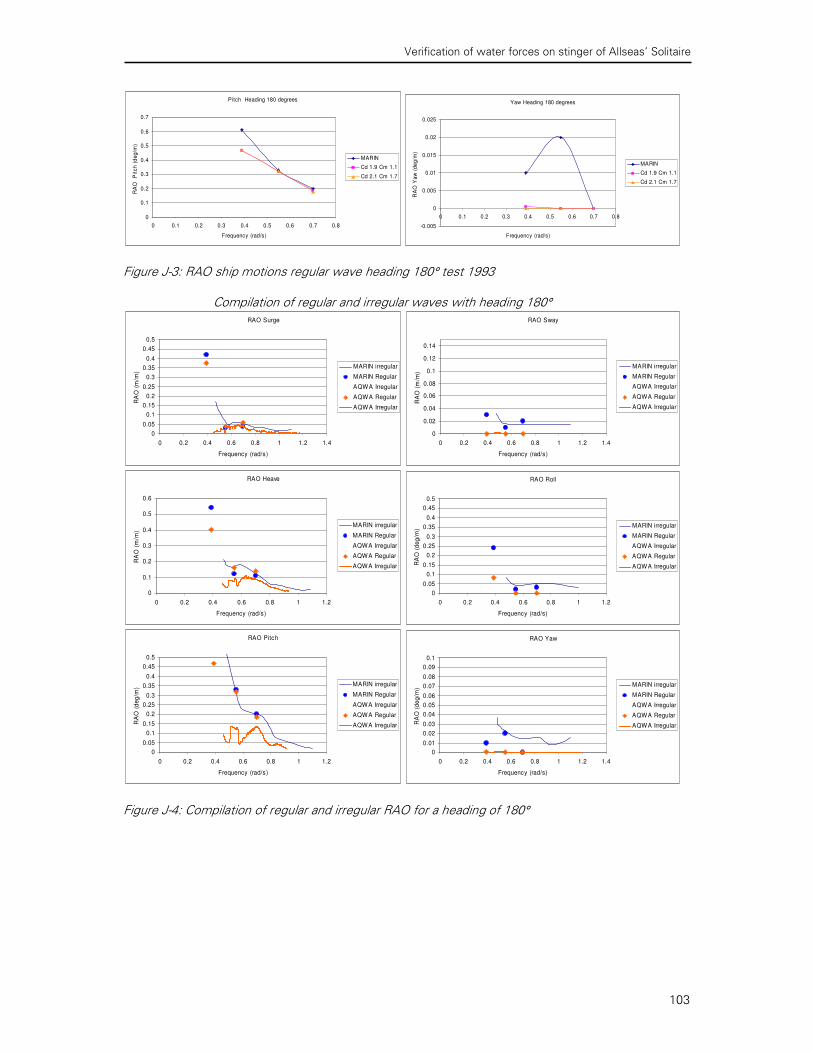
Verification of water forces on stinger of Allseas’ Solitaire
103
Pitch Heading 180 degrees
0
0.1
0.2
0.3
0.4
0.5
0.6
0.7
0 0.1 0.2 0.3 0.4 0.5 0.6 0.7 0.8
Frequency (rad/s)
RA
O
Pit
ch
(d
eg
/m)
MARIN
Cd 1.9 Cm 1.1
Cd 2.1 Cm 1.7
Yaw Heading 180 degrees
-0.005
0
0.005
0.01
0.015
0.02
0.025
0 0.1 0.2 0.3 0.4 0.5 0.6 0.7 0.8
Frequency (rad/s)
RA
O Y
aw
(d
eg
/m)
MARIN
Cd 1.9 Cm 1.1
Cd 2.1 Cm 1.7
Figure J-3: RAO ship motions regular wave heading 180° test 1993
Compilation of regular and irregular waves with heading 180° RAO Surge
0
0.05
0.1
0.15
0.2
0.25
0.3
0.35
0.4
0.45
0.5
0 0.2 0.4 0.6 0.8 1 1.2 1.4
Frequency (rad/s)
RA
O (
m/m
)
MARIN irregular
MARIN Regular
AQWA Irregular
AQWA Regular
AQWA Irregular
RAO Sway
0
0.02
0.04
0.06
0.08
0.1
0.12
0.14
0 0.2 0.4 0.6 0.8 1 1.2 1.4
Frequency (rad/s)
RA
O (
m/m
)
MARIN irregular
MARIN Regular
AQWA Irregular
AQWA Regular
AQWA Irregular
RAO Heave
0
0.1
0.2
0.3
0.4
0.5
0.6
0 0.2 0.4 0.6 0.8 1 1.2
Frequency (rad/s)
RA
O (
m/m
)
MARIN irregular
MARIN Regular
AQWA Irregular
AQWA Regular
AQWA Irregular
RAO Roll
0
0.05
0.1
0.15
0.2
0.25
0.3
0.35
0.4
0.45
0.5
0 0.2 0.4 0.6 0.8 1 1.2
Frequency (rad/s)
RA
O (
de
g/m
)
MARIN irregular
MARIN Regular
AQWA Irregular
AQWA Regular
AQWA Irregular
RAO Pitch
0
0.05
0.1
0.15
0.2
0.25
0.3
0.35
0.4
0.45
0.5
0 0.2 0.4 0.6 0.8 1 1.2
Frequency (rad/s)
RA
O (
de
g/m
) MARIN irregular
MARIN Regular
AQWA Irregular
AQWA Regular
AQWA Irregular
RAO Yaw
0
0.01
0.02
0.03
0.04
0.05
0.06
0.07
0.08
0.09
0.1
0 0.2 0.4 0.6 0.8 1 1.2 1.4
Frequency (rad/s)
RA
O (
de
g/m
)
MARIN irregular
MARIN Regular
AQWA Irregular
AQWA Regular
AQWA Irregular
Figure J-4: Compilation of regular and irregular RAO for a heading of 180°

Verification of water forces on stinger of Allseas’ Solitaire
104
Regular Heading 225°°°°
Surge Heading 225 degrees
0
0.05
0.1
0.15
0.2
0.25
0.3
0.35
0.4
0.45
0 0.1 0.2 0.3 0.4 0.5 0.6 0.7 0.8
Frequency (rad/s)
RA
O S
urg
e (
m/m
)
MARIN
Cd 1.9 Cm 1.1
Cd 2.1 Cm 1.7
Sway Heading 225 degrees
0
0.05
0.1
0.15
0.2
0.25
0.3
0.35
0.4
0.45
0 0.1 0.2 0.3 0.4 0.5 0.6 0.7 0.8
Frequency (rad/s)
RA
O S
wa
y (
m/m
)
MARIN
Cd 1.9 Cm 1.1
Cd 2.1 Cm 1.7
Heave Heading 225 degrees
0
0.1
0.2
0.3
0.4
0.5
0.6
0.7
0.8
0.9
0 0.1 0.2 0.3 0.4 0.5 0.6 0.7 0.8
Frequency (rad/s)
RA
O H
ea
ve
(m
/m)
MARIN
Cd 1.9 Cm 1.1
Cd 2.1 Cm 1.7
Roll Heading 225 degrees
-0.5
0
0.5
1
1.5
2
2.5
3
3.5
0 0.1 0.2 0.3 0.4 0.5 0.6 0.7 0.8
Frequency (rad/s)
RA
O R
oll
(de
g/m
)
MARIN
Cd 1.9 Cm 1.1
Cd 2.1 Cm 1.7
Pitch Heading 225 degrees
0
0.1
0.2
0.3
0.4
0.5
0.6
0 0.1 0.2 0.3 0.4 0.5 0.6 0.7 0.8
Frequency (rad/s)
RA
O P
itc
h (
de
g/m
)
MARIN
Cd 1.9 Cm 1.1
Cd 2.1 Cm 1.7
Yaw Heading 225 degrees
0
0.05
0.1
0.15
0.2
0.25
0.3
0.35
0 0.1 0.2 0.3 0.4 0.5 0.6 0.7 0.8
Frequency (rad/s)
RA
O Y
aw
(d
eg/m
)
MARIN
Cd 1.9 Cm 1.1
Cd 2.1 Cm 1.7
Figure J-5: RAO ship motions regular wave heading 225° test 1993

Verification of water forces on stinger of Allseas’ Solitaire
105
Regular Heading 270°°°°
Surge Heading 270 degrees
-0.005
0
0.005
0.01
0.015
0.02
0.025
0.03
0.035
0.04
0.045
0 0.1 0.2 0.3 0.4 0.5 0.6 0.7 0.8
Frequency (rad/s)
RA
O S
urg
e (
m/m
)
MARIN
Cd 1.9 Cm 1.1
Cd 2.1 Cm 1.7
Sway Heading 270 degrees
0
0.1
0.2
0.3
0.4
0.5
0.6
0.7
0.8
0.9
0 0.1 0.2 0.3 0.4 0.5 0.6 0.7 0.8
Frequency (rad/s)
RA
O S
wa
y (
m/m
)
MARIN
Cd 1.9 Cm 1.1
Cd 2.1 Cm 1.7
Heave Heading 270 degrees
0
0.2
0.4
0.6
0.8
1
1.2
0 0.1 0.2 0.3 0.4 0.5 0.6 0.7 0.8
Frequency (rad/s)
RA
O
He
av
e (
m/m
)
MARIN
Cd 1.9 Cm 1.1
Cd 2.1 Cm 1.7
Roll Heading 270 degrees
0
0.5
1
1.5
2
2.5
3
3.5
4
4.5
0 0.1 0.2 0.3 0.4 0.5 0.6 0.7 0.8
Frequency (rad/s)R
AO
Ro
ll (d
eg
/m)
MARIN
Cd 1.9 Cm 1.1
Cd 2.1 Cm 1.7
Pitch Heading 270 degrees
0
0.1
0.2
0.3
0.4
0.5
0.6
0 0.1 0.2 0.3 0.4 0.5 0.6 0.7 0.8
Frequency (rad/s)
RA
O P
itc
h (
de
g/m
)
MARIN
Cd 1.9 Cm 1.1
Cd 2.1 Cm 1.7
Yaw Heading 270 degrees
-0.05
0
0.05
0.1
0.15
0.2
0.25
0.3
0.35
0.4
0.45
0 0.1 0.2 0.3 0.4 0.5 0.6 0.7 0.8
Frequency (rad/s)
RA
O Y
aw
l (d
eg
/m)
MARIN
Cd 1.9 Cm 1.1
Cd 2.1 Cm 1.7
Figure J-6: RAO ship motions regular wave heading 270° test 1993
Verification of water forces on stinger of Allseas’ Solitaire
106

Verification of water forces on stinger of Allseas’ Solitaire
107
Appendix K: RAO ship motions MARIN test 2000
Regular wave tests heading 70°°°°
RAO Surge
0
0.1
0.2
0.3
0.4
0 0.2 0.4 0.6 0.8 1 1.2
Frequency (rad/s)
RAO(m/m)
MARIN
Cd 1.9 Cm 1.1
Cd 2.1 Cm 1.7
RAO Sway
0
0.2
0.4
0.6
0.8
0 0.2 0.4 0.6 0.8 1 1.2
Frequency (rad/s)
RA
O (
m/m
)
MARIN
Cd 1.9 Cm 1.1
Cd 2.1 Cm 1.7
RAO Heave
0
0.2
0.4
0.6
0.8
1
0 0.2 0.4 0.6 0.8 1 1.2
Frequency (rad/s)
RA
O (
m/m
)
MARIN
Cd 1.9 Cm 1.1
Cd 2.1 Cm 1.7
RAO Roll
0
0.8
1.6
2.4
3.2
0 0.2 0.4 0.6 0.8 1 1.2
Frequency (rad/s)
RA
O (
de
g/m
)
MARIN
Cd 1.9 Cm 1.1
Cd 2.1 Cm 1.7
RAO Pitch
0
0.2
0.4
0.6
0.8
1
0 0.2 0.4 0.6 0.8 1 1.2
Frequency (rad/s)
RA
O (
de
g/m
)
MARIN
Cd 1.9 Cm 1.1
Cd 2.1 Cm 1.7
RAO Yaw
0
0.15
0.3
0.45
0.6
0 0.2 0.4 0.6 0.8 1 1.2
Frequency (rad/s)
RA
O (
de
g/m
)
MARIN
Cd 1.9 Cm 1.1
Cd 2.1 Cm 1.7
Figure K-1: RAO ship motions regular wave heading 70° test 2000
Irregular wave heading 70°°°°
Standard deviations
Standard Deviation
0.00
0.05
0.10
0.15
0.20
0.25
0.30
0.35
0.40
0.45
0.50
Surge (m) Sway (m) Heave (m)
Me
tre
s MARIN
Cd 1.9 Cm 1.1
Cd 2.1 Cm 1.7

Verification of water forces on stinger of Allseas’ Solitaire
108
Standard Deviation
0.00
0.10
0.20
0.30
0.40
0.50
0.60
0.70
Roll (deg) Pitch (deg) Yaw (deg)
De
gre
es MARIN
Cd 1.9 Cm 1.1
Cd 2.1 Cm 1.7
Figure K-2: Standard deviation ship motions irregular wave heading 70° test 2000
Response Amplitude Operators
RAO Surge
0
0.05
0.1
0.15
0.2
0.25
0.3
0.35
0.4
0 0.2 0.4 0.6 0.8 1 1.2
Frequency (rad/s)
RA
O (
m/m
)
MARIN
AQWA vessel
Cd 1.9 Cm 1.1
Cd 2.1 Cm 1.7
Poly. (Cd 1.9 Cm 1.1)
Poly. (Cd 2.1 Cm 1.7)
RAO Sway
0
0.1
0.2
0.3
0.4
0.5
0.6
0.7
0.8
0.9
1
0 0.2 0.4 0.6 0.8 1 1.2
Frequency (rad/s)
RA
O (
m/m
)
MARIN
AQWA vessel
Cd 1.9 Cm 1.1
Cd 2.1 Cm 1.7
Poly. (Cd 1.9 Cm 1.1)
Poly. (Cd 2.1 Cm 1.7)
RAO Heave
0
0.2
0.4
0.6
0.8
1
0 0.2 0.4 0.6 0.8 1 1.2
Frequency (rad/s)
RA
O (
m/m
)
MARIN
AQWA Vessel
Cd 1.9 Cm 1.1
Cd 2.1 Cm 1.7
Avg. Cd 1.9 Cm 1.1
Avg. Cd 2.1 Cm 1.7
RAO Roll
0
0.5
1
1.5
2
0 0.2 0.4 0.6 0.8 1 1.2
Frequency (rad/s)
RA
O (
de
g/m
)
MARIN
AQWA Vessel
Cd 1.9 Cm 1.1
Cd 2.1 Cm 1.7
Avg. Cd 1.9 Cm 1.1
Avg. Cd 2.1 Cm 1.7
RAO Pitch
0
0.1
0.2
0.3
0.4
0.5
0.6
0.7
0.8
0.9
1
0 0.2 0.4 0.6 0.8 1 1.2
Frequency (rad/s)
RA
O (
de
g/m
)
MARIN
AQWA Vessel
Cd 1.9 Cm 1.1
Cd 2.1 Cm 1.7
Poly. (Cd 1.9 Cm 1.1)
Poly. (Cd 2.1 Cm 1.7)
RAO Yaw
0
0.05
0.1
0.15
0.2
0.25
0.3
0.35
0.4
0.45
0.5
0 0.2 0.4 0.6 0.8 1 1.2
Frequency (rad/s)
RA
O (
de
g/m
)
MARIN
AQWA Vessel
Cd 1.9 Cm 1.1
Cd 2.1 Cm 1.7
Poly. (Cd 1.9 Cm 1.1)
Poly. (Cd 2.1 Cm 1.7)
Figure K-3: RAO ship motions irregular wave heading 70° test 2000
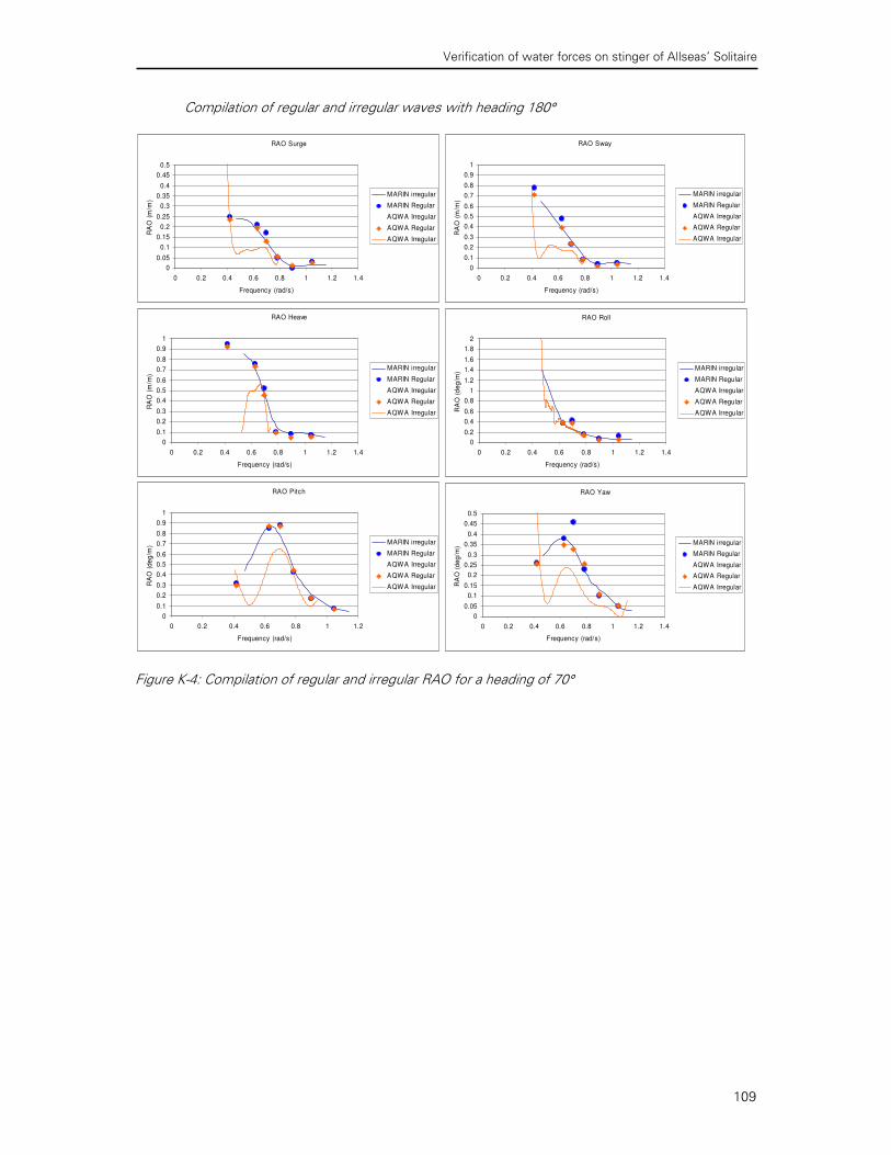
Verification of water forces on stinger of Allseas’ Solitaire
109
Compilation of regular and irregular waves with heading 180°
RAO Surge
0
0.05
0.1
0.15
0.2
0.25
0.3
0.35
0.4
0.45
0.5
0 0.2 0.4 0.6 0.8 1 1.2 1.4
Frequency (rad/s)
RA
O (
m/m
)
MARIN irregular
MARIN Regular
AQWA Irregular
AQWA Regular
AQWA Irregular
RAO Sway
0
0.1
0.2
0.3
0.4
0.5
0.6
0.7
0.8
0.9
1
0 0.2 0.4 0.6 0.8 1 1.2 1.4
Frequency (rad/s)
RA
O (
m/m
)
MARIN irregular
MARIN Regular
AQWA Irregular
AQWA Regular
AQWA Irregular
RAO Heave
0
0.1
0.2
0.3
0.4
0.5
0.6
0.7
0.8
0.9
1
0 0.2 0.4 0.6 0.8 1 1.2 1.4
Frequency (rad/s)
RA
O (
m/m
)
MARIN irregular
MARIN Regular
AQWA Irregular
AQWA Regular
AQWA Irregular
RAO Roll
0
0.2
0.4
0.6
0.8
1
1.2
1.4
1.6
1.8
2
0 0.2 0.4 0.6 0.8 1 1.2 1.4
Frequency (rad/s)R
AO
(d
eg
/m)
MARIN irregular
MARIN Regular
AQWA Irregular
AQWA Regular
AQWA Irregular
RAO Pitch
0
0.1
0.2
0.3
0.4
0.5
0.6
0.7
0.8
0.9
1
0 0.2 0.4 0.6 0.8 1 1.2
Frequency (rad/s)
RA
O (
de
g/m
) MARIN irregular
MARIN Regular
AQWA Irregular
AQWA Regular
AQWA Irregular
RAO Yaw
0
0.05
0.1
0.15
0.2
0.25
0.3
0.35
0.4
0.45
0.5
0 0.2 0.4 0.6 0.8 1 1.2 1.4
Frequency (rad/s)
RA
O (
de
g/m
)
MARIN irregular
MARIN Regular
AQWA Irregular
AQWA Regular
AQWA Irregular
Figure K-4: Compilation of regular and irregular RAO for a heading of 70°

Verification of water forces on stinger of Allseas’ Solitaire
110

Verification of water forces on stinger of Allseas’ Solitaire
111
Appendix L: Test set up
As stated in the recommendation of this thesis, a prototype test will give a more accurate verification
data as from a scale model test. The main reasons are no influence of scale effects and real life sea
conditions. After a test at sea with the Solitaire in real life, AQWA can be verified accurate.
To measure the forces and moment on the stinger the possibilities are limited. Below here the main
configuration of the stinger is given, with the cantilever and the main hinge point.
Figure L-1: Test set up for measuring force on stinger
Measuring at the main hinge point is difficult and installing a measuring device is difficult and costly.
Section 2 is attached to the Cantilever by wires, which run along winches. At the end of the wires in
the cantilever is the forces in this wires is measured already at the moment, but these forces are not
logged. A data logger had to be attached to this measuring device.
The most important moment to know for the stinger is the moment around the y-axis. The force
measured by the wires can be transformed by a moment around the main hinge. The wires will pick
up the total moment around the main hinge. This moment can also be calculated by AQWA. It is
difficult to divide the wire force in a Fx and Fz force. For the force in y direction also no
measurements can take place, but this force will not be of great significance.
During these measurement of the forces in the wires the ship motions have to be logged
simultaneously. This way the same approach as in this thesis can be used. First the ship motions
have top calibrated in AQWA to coincide with the ship motions measured and then the stinger My
moment can be compared.
For gathering the influence of the drag force and current test has to be done. From these test the
drag coefficient can be verified, which is an important coefficient for the total Morison force.
Comparing the AQWA results with these current test will say something about the magnitude of
interference in the stinger. This interference can reduce the drag of the stinger and can be of great
significance. A sea condition can be described by an irregular wave condition. This is the other test to
compare the stinger moment around the y-axis.
Cantilever
Wires
Main
Hinge