fluid mechanics prof. s. k. som department of mechanical...

Fluid Mechanics Prof. S. K. Som

Department of Mechanical Engineering Indian Institute of Technology, Kharagpur

Lecture - 33

Application of Viscous Flow Through pipes Part – I

Good morning, I welcome you all to this session of fluid mechanics. So, today we will be

discussing the topic application of viscous flow through pipes. Now, last class we have

solved the Navier-Stokes equation; equations of motions in parallel flows, where we

have assumed one thing that flow is laminar. And we have reduced the expression for

velocity profile and the flow rate and the corresponding pressure drop.

Now, there are two kinds of flow in a viscous flow; one is a laminar flow, another is

turbulent flow. So, we will come across this laminar, turbulent flow differences

afterwards; but now just in a short you must know that when the fluid velocity exceeds

some value for a given fluid under a given flow condition, the flow becomes turbulent.

So, turbulent flow in short is that the flow becomes irregularly fluctuating with time; that

flow becomes an irregular functions of time, flow is never a steady one.

So, at any point the flow velocity becomes an irregular function of time, and these

variations of flow velocity with time is random. So therefore, we cannot have a steady

flow that way and another thing is that if there is a one dimensional flow; that means,

flow is taking place in one dimensional, in a laminar flow all the fluid particles moving

in that direction. So, stream lines are parallel to each other. So, planes are gliding over

each other.

But in a turbulent flow what happens? There is a fluctuating velocities with time and

more over the cross component; even if there is no bulk flow, there is a flow generated,

the value is very small; the flow velocity generated in orthogonal directions to that of the

direction of flow. So, these are the characteristic features of turbulent flow. The flow

becomes irregularly fluctuating with time. But one thing you must know at this junction

that these fluctuations are random, so that the statistical description is possible; that

means this variation may be brought down by the laws of probability.

So, that an average velocity is defined; a time average velocity in turbulent flow which is

steady, if the main flow is steady or this average flow velocity is in one direction only, if

the flow is one dimensional. But strictly speaking, the flow at any point has got a three

dimensional nature, and this is irregularly fluctuating with time; this is a turbulent flow.

Usually all flows in nature are turbulent flow. So, laminar flow occurs with extremely

small velocity; extremely small values of velocity which are not usually encountered in

practical applications.

So most important thing in turbulent flow for engineers is that, due to the turbulent flow

the fluid friction interaction between the fluid to solid and layer to layer fluid friction is

enhanced; that means it offers more resistance for a given flow, which if you again

transmit to a very hardware language; that means for a given flow rate through a duct,

the pressure drop across a length of the duct is much more than that of a laminar; that

means if you make an analytical solutions from the laminar flow, then you will get a less

value that you encountered in practice if the flow is turbulent.

So therefore, there the solution is not very easy. Nowadays with the advent of

computational fluid dynamics or the computational mathematics applied in fluid

mechanics problems, we can solve the turbulent flow situations; but still at certain stage,

the theoretical solutions or the computational solutions or numerical solutions need some

help from experiments; that means they require some empirically information and you

nowadays the closer models, which have been developed for solving the turbulent flow

known as turbulence model; they are based on the empirical constant.

So therefore, a turbulent flow solution is not very easy. So in this class, we will discuss

this type of applications in turbulent flow where an engineer is really interested, who

knowing for given flow through a pipe, what will be the pressure drop over a given

length and if I know the pressure drop, I can find out what is the pumping power

required to force the fluid through the pipe; or if I know the flow rate, if I know the

pumping power I can find out what diameter of the pipe should be.

So, these types of practical problems of turbulent viscous flow through pipes are solved

in a very routine manner and conventional manner, which is not fully theory, not fully

experiment, is a combination of theoretical analysis with experimental information

known as semi-empirical approach and will be done in this class. So, let us now see how

we can do it.

(Refer Slide Time: 05:00)

So, first we recall again the friction factor concept. So, now we know; first we start with

for a flow through a pipe. Let us consider this section is dedicated to viscous flow

through a pipe and a friction if turbulent flow; viscous turbulent flow, this is the pipe.

Now let this is the axis of the pipe. We take a control volume. Now let us consider a

control volume whose surfaces are coinciding with the pipes surfaces. Let us take the

control volume like this. Now we see that, what are the forces acting on it; one is the

shear force. This is the tau w acting in the surface, the same direction, because this is the

surface gliding with the cylinder surface, the control volume.

So, flow is taking place in these directions. So therefore, shear stress in this direction; tau

w acting on this throughout the surface. So, pressure is acting at this cross-section, let P.

Let this is the piezometric pressure. We consider the pressure, static pressure plus the

equivalent pressure rate due to the elevation rate; that is the potential from a reference

data. Why we take it. Because in case of vertical pipe or a pipe inclined in a vertical

plane, the difference between the pressures from one section to another one section is the

static pressure difference in energy static pressure plus the change in the potential head,

which takes care of the gravity forces into account. This type of analysis we have already

made.

So, there is a loss in piezometric pressure p star. Let this is the length of the control

volume or the fluid element as you tell. So therefore, this is the loss over the length L in

the piezometric pressure. So, this difference will be the difference in piezometric

pressures, which is the difference in static pressure if the pipe is horizontal. Now simply

if we make a force balance considering the inertia force to be 0; you know a parallel flow

through a tube or a pipe, the inertia force is 0, we discussed it earlier. So, if we make the

force balance of this fluid element; that means the fluid element is in equilibrium with

the pressure and shear forces, then we can write this if we consider the cross-sectional

area as A. If we consider the perimeter, weighted perimeter is S; this is not for a pipe

also this is valued for any duct so that weighted perimeter is S.

Then we can write this p star into A this side minus p star minus delta star, very simple,

into A. This is the net forced in this direction due to pressure force must be balanced the

opposite direction force; that is tau w into the surface area; that means, the weighted

perimeter times the L; L is the length, that is the surface area. So, simply we get from

here tau w is what; tau w is delta p star, any problem you just ask me, S into L. So this is

the shear stress, where S into L is the weighted perimeter into the length; that is the total

surface area S into L over which the shear stress acts. So, this is alright. Now if we

define a hydraulic diameter D h, how do you define the hydraulic diameter? We have

defined a hydraulic diameter which is defined as 4 times the cross-sectional area divided

by weighted perimeter.

So, this is the general definition of hydraulic diameter in relation to flow through a duct

internal flow 4A by S. So therefore, we can write A by S as one-fourth D h. So therefore,

this becomes is equal to 1 by 4 D h A by S is that D h by L into delta p star. So, it is

alright with respect to this. We get an expression relating shear stress to pressure drop,

piezometric pressure drop; that means it takes care of the change in the potential in terms

of the equivalent pressure. In case of a horizontal duct it is the static pressure duct.

So, you see that shear stress is related to pressure drop which can be found out very

straightforward and simple application of force balance on a fluid element when inertia

force is 0; that means physically it is because of the shear stress, there is a pressure drop.

So, there was no shear stress for an ideal fluid, there is no pressure drop from this section

to this section; that means at all sections pressure remains same for an ideal flow, you

know the energy also remain same. There is no dissipation of energy. So, therefore, the

shear stress is related to pressure drop by this expression.


Now if we go one step forward and if we recall earlier class, we discussed that

coefficient of skin friction or skin friction coefficient C f is defined as shear stress at the

wall divided by the dynamic head rho V square; that we defined that for any type of fluid

flow, whether it is an internal flow that flow through a duct or an external flow pass

bodies, this skin friction coefficient a parameter dimensional is defined as the shear

stress at the wall; that means, at the solid and fluid adjacent, adjacent to solid and fluid.

So tau w divided by half rho V square where this V is the reference velocity, which in

case of internal flow or flow through duct is the average flow velocity. So, if I write this

definition and put this value of tau w it becomes 1 by 4 into D h by L into delta p star by

half rho V square. This C f is known as, this way again I write C f is equal to one-fourth

D h by L; all dimensionless parameter D h by L and delta p star divided by dynamic head

half rho V square.


So, this way I write this C f is known as Fanning’s friction factor; Fanning is the person,

Fanning’s friction factor. This C f derived from the basic definition of skin friction

coefficient in terms of a piezometric pressure drop or static pressure drop as you tell in

case of internal flow and the hydraulic diameter is known as Fanning’s friction factor;

that means it is derived from the basic equation of skin friction coefficient in terms of the

shear stress at the wall, but then it is expressed in terms of the pressure drop.

Since we know the relationship between shear stress and pressure drop derived from the

force balance of a fluid element, then final expression stands as skin friction coefficient

in terms of the pressure drop and the hydraulic diameter, and this is the average flow

velocity in case of an internal flow through a duct. This is the average flow velocity

whose definition is that Q by cross-sectional area. So, if cross-sectional area remains

same in the direction of the flow the average velocity remains same, because Q always

remains same under steady condition.

So if average area cross-sectional area changes, the average velocity changes. So, this is

the definition of Fanning’s friction coefficient. So, Darcy defines a friction coefficient f.

This is Darcy’s friction coefficient, another person friction coefficient who defined the

friction coefficient if as doing however, with 1 by 4 he left this 1 4 simply he defined D h

by L times the delta p star divided by the half rho V square, which means that f is

nothing but 4 C f; that means, if you multiply 4 with the Fanning’s friction coefficient

you get a friction coefficient f, f is D h by L delta p star half rho V square. So, this is the

definition of the Darcy’s friction coefficient. This equation defines Fanning’s friction

factor; this equation defines Darcy’s friction coefficient of friction factor whatever you

tell.

Now, this equation is actually represented in a different form; not f as this if we write

delta p star is f into L by D h into half rho V square. This equation becomes useful to the

practical engineers. What they do that if they can know the friction factor for a particular

flow from some handbook, from some chart or from some predetermined experimental

values, knowing the geometry of the duct they can find out what is the pressure drop for

a given length L; geometry means the hydraulic diameter is known, if he knows the flow

rate; that means if I know the flow rate, so I can find out what is the pressure drop.

From flow rate I can find out the average velocity knowing the geometry of the duct; that

means cross-sectional area. Then one can find out what is the pressure drop in the duct

and one can find out the corresponding power requirement; power requirement is now

simply delta p into Q. So, this is the amount of fluid flow rate and this is the pressure

drop over a given length. So, to force that fluid at this rate over a given length this power

is required.

So, I can know for a given flow rate through a given geometry of pipe; that means for a

given length and given diameter, what is the pressure drop and what is the power

required or other way if we know the power or pressure drop, I can find out what should

be the flow rate. So, this equation is very important in the applications of viscous flow

through a pipe. Now for a circular tube or pipe D h is the pipe diameter D, because 4

times cross-sectional area is pi D square by 4 divided by the weighted area, pipe is

flowing full; so pi D, so this D h becomes D. So therefore, this will be simply L by D.

So, now the problem falls down in knowing the values of the friction factor.


Now friction factor, if I come to the friction factor values in pipes. Now let us write the

friction factor; that means now, I will discuss the friction factor you will understand this

is the Darcy’s friction factor in pipes. Definition is like this delta p; delta p is equal to

this friction factor times L by D length to diameter ratio times what is delta P; it is L by

D into half rho V square dynamic, where V is the average velocity, where V is equal to

Q by A.

So, this has to be there always in front of your eyes; that means in front of you this

definition friction factor. Now this f now, first of all in laminar flow we have already

deduced the value of A. From exact solution we have found out C f is equal to 16 by Re

Reynolds number, where Re we have found out from the Hagen-Poiseuille solution in

the class rho VD by mu, if V is the average flow velocity in the direction of flow; that

means in axial direction of the pipe.

So, these combinations of the parameters dimensionally; this becomes a dimensionless

parameter, this typical combination rho VD by mu which is known as Reynolds number.

We have seen that tau w, but skin friction coefficient by half rho V square which is

nothing but C f, which is the Fanning’s friction factor here 16 by Re. So, f is equal to 64

by Re. So, it is a simple analytical relation we know, but in turbulent flow it is difficult to

develop that relationship from theory. But nowadays we are doing it with the head of

computational fluid dynamics and also experiments are being done to match it and even

the solutions of turbulent flow, as I have told earlier depends upon the experimental

information. So, they are generated basically from experiments.

Now first of all you have to know in a pipe flow, the flow becomes turbulent when this

Reynolds number as defined by this exceeds the value of 2000; that means Reynolds

number less than 2000, the flow is laminar. So this Reynolds number criteria for flow to

change from laminar to turbulent depends on flow to flow. So, this is the 2000 Reynolds

number below which the flow becomes laminar and above which the flow becomes

turbulent, this depends and this is only in case of pipe flow.

For different type of flow, the criteria for Reynolds number for flow changing from

laminar to turbulent is different; that means the values are different. But Reynolds

number is the dimensionless number which serves as the criteria for laminar to turbulent

flow. So considering water even at the ambient condition, if you take its value rho and

mu you can find out to maintain a 2000 value or below 2000 value to maintain a flow

laminar you require; even for a very small diameter, feasibly small diameter in

laboratory or in practice what is the value of V.

That means the extremely small value of flow velocity or extremely small value of D can

only make the Reynolds number less than 2000. For all practical applications of

moderately large value of D and moderately large value of V makes the flow Reynolds

number beyond 2000, so that flow becomes turbulent and the turbulent flow the value of

the friction factor of the shear stress changes. The shear stress that is the friction between

layer to layer of the fluid and that between fluids to solid is enhanced by the mixing in

the turbulent flow that I will discuss afterwards.

So turbulent flow the only thing you know, the flow resistance which is due to the

friction between the fluid layers or between the fluids to solid is increased; that means,

the viscosity is apparently increased. That is why a term apparent viscosity or A D

viscosity comes in case of turbulent flow. So therefore, the flow resistance is increased;

so pressure drop is increased for given flow in turbulent region. But there is not a single

equation by which one can feel the pressure drop and flow rate relationship or skin

friction coefficient f versus Reynolds number throughout the entire range of turbulent

flow; that means when the flow becomes Reynolds number becomes more than 2000. So,

a single formula will hold good. So in different ranges, different formulae are applicable.


So people likes Stanton, Nikuradse, you must know the name; Nikuradse they were

pioneers, and finally Moody is the man who documented in a very nice way in a figure

form, all the values of f versus Re for our use and which is of great use and a popular use

till today and is known as Moody’s diagram, which I will show you now.


This is the Moody’s diagram. This is what it is the friction factor versus Reynolds

number.

Now another fact I must tell you that it has been found that in laminar flow the friction

factor from analytical solutions of Navier-Stokes equation is a function of Reynolds

number only. But in turbulent flow, friction factor is a function of both Reynolds number

and the roughness factor; this roughness factor. So, usually in laminar flow the friction

factor is a function of Reynolds number and there is another type of pipe; that is smooth

pipe whose roughness is almost 0. So, there the frictional factor is a function of Reynolds

number.

But for all commercial pipes it has got roughness; roughness is measured in commercial

pipe by the size of the height of the protrusions at the surface. You know there are

several methods by which surface roughness is specified. So for all commercial pipes,

we know the surface roughness or other commercial pipes are specified by the surface

roughness; this is the linear dimension. This either is specified either by measurement of

surface roughness or by comparing the flow rate and pressure drop data of a commercial

pipe with those of a pipe, which were artificially the roughness is created by gluing sand

grain of uniform height so that this height; the measure of this height is the measure of

the roughness.

Actually a statistical average of the surface protrusion is the measure of the roughness of

a commercial pipe. So, for commercial pipe in turbulent flow region frictional factor is

function of roughness. But for any commercials pipe, if the flow region is or the flow

region is laminar it is a function of only Reynolds number. So only in case of turbulent

flow, the surface roughness comes at an influencing variable in friction factor.

The physical reason behind this is that, in case of laminar flow the surface the boundary

layer is so high, so that the surface protrusion cannot protrude over the boundary layer

because these things we have not come across so far. This does not make any

contribution to the velocity gradient at the wall to change as it is; so therefore, this is not

so in case of laminar flow. But in turbulent flow, the surface roughness is an influencing

parameter in changing the friction factor. It becomes the function of both Reynolds

number and surface roughness.


So now, this has been plotted nicely by Moody, this is known as Moody’s diagram. Here

the friction factor is the ordinate and this is the Reynolds number. This is plotted in a

large scale to cover a wide range and this ordinate is the dimensionless surface

roughness; that means surface roughness epsilon by the pipe diameter, epsilon by D

which is known as relative surface roughness.

So, now in laminar flow this is the equation f is equal to 64 by Re. Because we know we

have developed this from analytical solutions of Navier-Stokes equation; that is Hagen-

Poiseuille equation that C f is 16 by Re. So, f is 64 by Re. So, this is the laminar flow.

There is a discontinuity from laminar to turbulent start because as you come to this

laminar turbulent flow analysis, you will see; so just after the laminar flow immediately

the turbulent flow does not occur.

There is a transition zone through which the turbulent flow is setup and within this

transition zone everything is unpredictable. The flow oscillates from laminar to turbulent,

turbulent to laminar, so everything is very uncertain. So, there is a discontinuity in the

curve we will see now. This is for smooth pipe this curve; this curve is for smooth pipe.

So after that, you see the curves are branching of from the smooth pipe curves with the

increasing order of the roughness; so increasing order of the epsilon by D.

Now, one characteristic feature is that in turbulent flow for rough pipes you see after

some Reynolds number the curve becomes more or less parallel, which means the

friction factor becomes independent of the flow rate. Now here friction factor becomes

independent of the Reynolds number. Now if we defined the friction factor, you should

not confuse that the friction factor is decreasing with the Reynolds number does not

mean the pressure drop decreases with the flow rate. Because friction factor is defined as

how; how do you define the friction factor; f is, please tell me the definition of the

friction factor, f is how do you define f delta P; delta p D by L friction factor half rho V

square.

So you see when friction factor is inverse function, linear inverse function of Reynolds

number this means delta p is a single; that means, linear function of V. As you know

from the Hagen-Poiseuille solution delta P is a linear function of V. So, f becomes an

inverse function of V; so that friction factor decreases inversely with V. Here friction

factor becomes independent of Reynolds number; means friction factor becomes

independent of the Reynolds number; they have been independent of velocity because

Reynolds number if you write here, Reynolds number is rho VD by mu. So, for a

particular pipe Reynolds number change in Reynolds number means change in V; that

means pressure drop is proportional to V square; that means when this curves are

parallel, which means these are not functions of, the friction factor is not depended on

the Reynolds number means pressure drop is almost a function of V square.

So V square, V square cancelled. So, friction factor we get constant value. But before

that friction factor is an inverse function of Reynolds number; that means, delta p is a

function of V to power 1 to 2; not equal to 2. So, that this friction factor becomes an

inverse function. So, delta p always increases with the increase of V, but the power

represents how that friction factor will be constant or will be decreasing. If the power is

more than 2, it does not happen in fluid flow practice. Then friction factor increases with

the increasing Reynolds number, this does not happen so. This zone is known as rough

zone; that means pipe is completely rough.

Rough zone are fully turbulent zone where the friction factor is independent of Reynolds

number, pressure drop is proportional to V square and this portion where from this

smooth curve of different commercial pipes of different roughness branches are from the

smooth pipe, these portions rather is known as the critical tube. These are not very

important critical zone. Now what is important from the point of view of solving

problems or doing the industrial problem that one should read the value of friction factor

from this Moody’s diagram; that means if I know the roughness factor for a commercial

pipe, if I know what is the Reynolds number I can find out the friction factor? This curve

is hardly used because practical problems are associated with turbulent flow not with the

laminar flow. So, this is in all the Moody’s diagram.


Now come to the practical situations; so with this background, with this knowledge in

background, now I go one step forward that what are the different types of problem that a

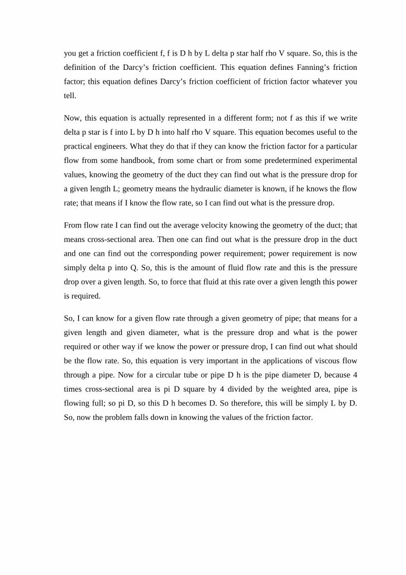
hydraulic engineer faces. There are typically three types of problem; one is that the flow

rate and pipe diameter are given. Find pressure loss over a giving length and the

corresponding power.

This type of first type of problem; this is very simple. The straightforward full level

problem; that means flow rate and pipe diameter are given; that means you know the

velocity; that means velocity is given and pipe diameter is given. Find the pressure loss

over a given length. Then the length is given, we have to find out the pressure drop over

a given length, straightforward application of this equation. When the velocity is given, I

can find out the Reynolds number rho VD by mu because V is given, D is given. So, for

what there are working fluid the work in fluid will be given that properties; the real

logical properties and I know Re. So, f has a function of Re.

If it is a smooth pipe otherwise a function of epsilon, I know the value of f a

straightforward I can find out delta p and I can find out the corresponding power Q into

delta p; this is the straightforward application of this. But the second and third kind of

problem is difficult relatively; why, because second kind of problem the head loss over a

given length of pipe of known diameter is given. Head loss means this one; that means

either you express in times of delta p or you express in times of head loss; that means,

delta p by rho g; that means sometimes we express this equation in terms of the pressure

drop as it was derived first or in terms of the head loss; head loss means loss of pressure

energy.

That means in terms of the pressure head; that means delta p by rho g; that means V

square by 2g. Then this part becomes velocity head. If dynamic head have rho V square,

it is per unit mass, this is the velocity head. So head loss over a given length is given;

that means length is given, head loss is given; that means delta p is given. Find the flow

rate and power required, you have to find out V. Why this is difficult; because when V is

unknown, we do not know even f. Because to calculate f from Moody’s diagram, to see

the Moody’s diagram we required the Reynolds number. Even if we require epsilon,

main variable is Reynolds number.

Velocity is not known beforehand, so Reynolds number is not known. So, there are two

unknowns. We do not know f we do not know V, because f is a function of V in turn to

Reynolds number. So, this type of problem cannot be solved straightforward, but it is

solved by iterative process; that means here what we do. We guess a friction factor first

and then we find out the first iteration velocity from known values of delta h or delta p

any way you write the equation.

Then this second iterative value of V is used to find out the Reynolds number and find

out the f from the Moody’s diagram, then use this f in this equation and find the second

iterative value of V and then again find out at that V, what is the second Reynolds

friction factor and see the convergence between this two. This way this is been iterative I

will show you an example. The third problem also is the similar type; the flow rate and

the loss of head over a given length are known. Find the diameter; that means this is

known. Flow rate is known means V is known, but diameter is unknown; that means in

this equation the diameter is unknown and diameter is unknown means friction factor is

unknown.

Because friction factor to know I have to know both flow rate or the average flow

velocity and the diameter. So if diameter is not known, flow rate is not known; then it

becomes an iterative problem. So, it has to be solved by iteration. But if the flow rate and

diameter and length are known and we have to find out delta h or delta p first class of

problem, this is a straightforward application. So, these three typical classes of problem

exist in pipe flow analysis; pipe flow problems.


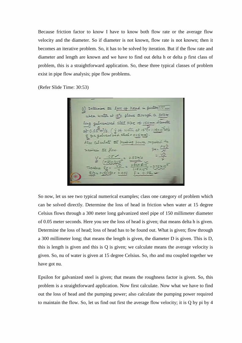
So now, let us see two typical numerical examples; class one category of problem which

can be solved directly. Determine the loss of head in friction when water at 15 degree

Celsius flows through a 300 meter long galvanized steel pipe of 150 millimeter diameter

of 0.05 meter seconds. Here you see the loss of head is given; that means delta h is given.

Determine the loss of head; loss of head has to be found out. What is given; flow through

a 300 millimeter long; that means the length is given, the diameter D is given. This is D,

this is length is given and this is Q is given; we calculate means the average velocity is

given. So, nu of water is given at 15 degree Celsius. So, rho and mu coupled together we

have got nu.

Epsilon for galvanized steel is given; that means the roughness factor is given. So, this

problem is a straightforward application. Now first calculate. Now what we have to find

out the loss of head and the pumping power; also calculate the pumping power required

to maintain the flow. So, let us find out first the average flow velocity; it is Q by pi by 4

D square the cross-sectional area. D is 150 millimeter 0.15 meter square. So, this

becomes 2.83 meter per second is V. So therefore, we first immediately calculate

Reynolds number since I know the diameter of the pipe, what is that 150 millimeter 0.15

meter, so V D by nu; rho VD by mu so that is equal to VD by nu. So, I get the Reynolds

number.

Now from Moody’s diagram with the relative roughness, here roughness is given

millimeter. So, to read Moody’s diagram I have to find out the relative roughness 0.001,

I find out f as 0.02 straightforward. This cannot be found from the figures that I have

shown because I have not drawn the numerical thing. So, the straight way you see the

Moody’s diagram it is given in each and every book. You straight find out the value of f.

So knowing this value of f, one can find out what is the loss of head and what is the

power required.


So f is 0.02; how can I find out then h f. So delta h is equal to what; you tell me f L by D

V square by 2g. So 0.02, what is L; L is 300 meter. So 300 and D is 0.15 meter L by D

into V square; V is 2.83 whole square 2 into 9.81. So, you straightforward get delta h and

this delta h is what 16.33 meter. Now power requirement is delta p into Q; delta p is rho

g times this; that means 10 to the power 3 into 9.81 into delta h. Delta h means delta p by

rho g in terms of the rate. So, head loss means the pressure loss delta p by rho g. So again

rho g, I multiplied with delta h or delta p into Q, what is the value of Q; so far I recollect

0.05. So, this gives watt. In terms of kilowatt, it is 8 kilowatt. So, this is the first category

of problem.


Now second category of problem you see; the second category of the problem is the

problem where the head loss is not to be calculated. Head loss is given, either flow rate

or diameter so that the friction factor is not known beforehand. For example, we see this

problem. Oil of kinematic viscosity 10 to the power minus 5 meter square per second;

this is the kinematic viscosity, power D is given, flows at a steady rate through a cast

iron pipe of 100 millimeter diameter, I am happy, the diameter is given and of 0.25

millimeter average surface roughness; surface roughness is given.

If the loss of head over a pipe length is 120 meter is 5 meter; that means loss of head is 5

meter and pipe length is given, L given, delta h given, this is the viscosity mu given, this

is D given and of 0.2 meter; that means, this is the epsilon given. So, what is not given;

what is the flow rate. So, I cannot find out directly, why; because here the same thing

that if I write this delta h is equal to f L by D V square by 2g then delta h is given, to find

out the flow rate I have to find out the average velocity because diameter is given,

But how can I find out average velocity, because friction is not known. To know the

friction factor I require Reynolds number. Again to know Reynolds number I require the

flow velocity. So when flow velocity is not given, I have told that if flow velocity and

diameter is not given then friction factor is not known beforehand. So, we cannot

straightforward use this ones and get the solution which is known as explicit method;

that means once you straightforward use the equation straightforward and get the

solution, that is the first category of problem but here we cannot do it.

So, what we do an iterative solutions how it is. First you calculate the surface roughness

0.0025; this is the relative surface roughness. Now then what happened; you guess a

value of f 0.026. You can ask me sir, how can I make a guess; you can make any guess.

But in the order of 0.02, 0.0 and this is the order of the friction factor; but depending

upon your guess, the number of iterative steps will depend. If you can make a correct

guess, the number of iteration will be less.

Usually what you do is that you should do that with this epsilon by D value, in a

moderate Reynolds number, you search a value of f from Moody’s diagram; just an

arbitrary moderate Reynolds number in the turbulent flow. For example 10,000; with this

relative roughness I guess a value which is 0.026. Now with this guess value first trial I

can straightforward use the delta h value and can find out 5 is equal to point with this

guess value, this V square; that means, I can find out the value of V.


And this value of V, first iterations we will keep V is equal to 1.773 meter per second;

with this V, I again try to find out the value of f. Because f was taken as guess value,

then I want to improve the value of f, how; with this first iteration guess iteration number

of iteration you write here, first iteration I find the value of Reynolds number; that means

rho V, first iterative value D by mu. So, that is VD by nu; nu is given. So, this becomes

is equal to 1.773 10 to the power 4. So, you get the value of the Reynolds number.

With this Reynolds number and the average surface roughness or the epsilon by D, the

relative surface roughness 0.0025 you get a value of f as 0.0316. With this f, you then

find out the updated values of V; next step values of V; that means, again you use this f, f

is equal to L by D. What is delta h is equal to 0.0316 into L by D 120 by 0.10 same into

V square; the second iterative value 2 divided 2 into 9.81, which gives the second

iterative value, second V square, sorry how can I tell; that is first iterative value square is

there V 2 square. So, I get second iterative value V 2; it is V 2 square. So, V 2 is second

iterative value is 1.608. With this V 2, I find the Reynolds number as 1.608 10 to the

power 4.

You calculate rho VD by mu. Then with this Reynolds number I see that my friction

factor becomes 0.0, what is that value; that with this Reynolds number I find 0.0318.

Now you see the difference between this two is very small; it is 0.63 percent. Where you

will stop; in practice, you will stop where you see that your results are fairly accurate and

you will have to take a judgment. If it is below 1 percent, the change in friction factor

will definitely tell the convergence is achieved; that means, we declare the final value of

1.608 meter per second. So, you want to know flow rate. I can tell you, 1.608 into pi D

square by 4. What is D square; what is D 0.1, 0.1 square divided by 4. So, this will be

0.013 meter Q per second.

So you see therefore, this category of problem where the diameter is not given. Then we

solve this category of problem where the flow rate is not given or where the diameter is

not given; that means to find out the diameter or find out the flow rate, we will have to

make iterations. We first guess a friction factor then find out either the velocity average

velocity or the flow rate; same thing or the diameter and then the first iteration, then this

values of diameter or the flow rate whatever is to be found out. If one is to be found out,

other is to be given. We update the Reynolds number or you find the Reynolds number

and update the value of friction factor and then we compare it with the guess value.

If we get exactly the guess value; that means your guess is perfectly correct and that is

the answer. But if is not sure, then with that updated value of friction factor you again

calculate that diameter of velocity, which you have to calculate either of the two. Then

again you update the friction factor and this way you see the convergence in the iterative

procedure. But the first category where you have to find out the head loss or the pressure

drop, there you do not have to do that; because there you have L, D, V all are in your

hand, beforehand to calculate.

You straightforward use this equation once for all and get the value of delta p or delta h

and finally, the pressure drop. So, these three classes of problems are straightforward.

First in practice by an engineer, and they are solved like that; that means with the

knowledge of friction factor, which is given are documented in a figure like Moody’s

diagram or sometimes from a chart; that means you use a chart or Moody’s diagram.

This is full of experimental or empirical information and then you use your theoretical

equations developed from the force balance of a fluid element; that means, the pressure

drop connecting the length and diameter of the pipe and the average velocity; that is flow

rate by area through this friction factor and you find out the parameters that you are

going to determine. So, today up to this.

Thank you.

Summary:


Problems:



fluid mechanics prof. s. k. som department of mechanical...

Documents