fluid mechanics and machinery laboratoryfiles.kluceb.webnode.in/200000041-72634735b1/fm...

1

FLUID MECHANICS AND MACHINERY LABORATORY

STUDENTS REFERENCE MANUAL

K.L.UNIVERSITY

DEPARTMENT OF CIVIL ENGINEERING

Compiled By

P.SUNDARA KUMAR, M.Tech (PhD) Associate Professor

2

Preface

In most of the engineering institutions, the laboratory course forms an integral

form of the basic course in Fluid Mechanics at undergraduate level. The experiments to

be performed in a laboratory should ideally be designed in such a way as to reinforce the

understanding of the basic principles as well as help the students to visualize the various

phenomenon encountered in different applications.

The objective of this manual is to familiarize the students with practical skills,

measurement techniques and interpretation of results. It is intended to make this manual

self contained in all respects, so that it can be used as a laboratory manual. In all the

experiments, the relevant theory and general guidelines for the procedure to be followed

have been given. Tabular sheets for entering the observations have also been provided in

each experiment while graph sheets have been included wherever necessary.

It is suggested that the students should complete the computations, is the

laboratory itself. However the students are advised to refer to the relevant text before

interpreting the results and writing a permanent discussion. The questions provided at the

end of each experiment will reinforce the students understanding of the subject and also

help them to prepare for viva-voce exams.

Author

3

GENERAL INSTRUCTIONS TO STUDENTS

The purpose of this laboratory is to reinforce and enhance your understanding of

the fundamentals of Fluid mechanics and Hydraulic machines. The experiments

here are designed to demonstrate the applications of the basic fluid mechanics

principles and to provide a more intuitive and physical understanding of the

theory. The main objective is to introduce a variety of classical experimental and

diagnostic techniques, and the principles behind these techniques. This laboratory

exercise also provides practice in making engineering judgments, estimates and

assessing the reliability of your measurements, skills which are very important in

all engineering disciplines.

Read the lab manual and any background material needed before you come to the

lab. You must be prepared for your experiments before coming to the lab. In

many cases you may have to go back to your fluid mechanics textbooks to review

the principles dealt with in the experiment.

Actively participate in class and don’t hesitate to ask questions. Utilize the

teaching assistants. You should be well prepared before coming to the laboratory,

unannounced questions may be asked at any time during the lab.

Carelessness in personal conduct or in handling equipment may result in serious

injury to the individual or the equipment. Do not run near moving machinery.

Always be on the alert for strange sounds. Guard against entangling clothes in

moving parts of machinery.

Students must follow the proper dress code inside the laboratory. To protect

clothing from dirt, wear a lab apron. Long hair should be tied back.

Calculator, graph sheets and drawing accessories are mandatory.

In performing the experiments, proceed carefully to minimize any water spills,

especially on the electric circuits and wire.

Make your workplace clean before leaving the laboratory. Maintain silence, order

and discipline inside the lab.

cell phones are not allowed inside the laboratory.

Any injury no matter how small must be reported to the instructor immediately.

Wish you a nice experience in this lab!

4

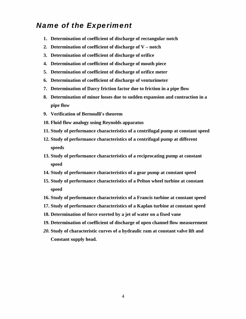
Name of the Experiment

1. Determination of coefficient of discharge of rectangular notch

2. Determination of coefficient of discharge of V – notch

3. Determination of coefficient of discharge of orifice

4. Determination of coefficient of discharge of mouth piece

5. Determination of coefficient of discharge of orifice meter

6. Determination of coefficient of discharge of venturimeter

7. Determination of Darcy friction factor due to friction in a pipe flow

8. Determination of minor losses due to sudden expansion and contraction in a

pipe flow

9. Verification of Bernoullis theorem

10. Fluid flow analogy using Reynolds apparatus

11. Study of performance characteristics of a centrifugal pump at constant speed

12. Study of performance characteristics of a centrifugal pump at different

speeds

13. Study of performance characteristics of a reciprocating pump at constant

speed

14. Study of performance characteristics of a gear pump at constant speed

15. Study of performance characteristics of a Pelton wheel turbine at constant

speed

16. Study of performance characteristics of a Francis turbine at constant speed

17. Study of performance characteristics of a Kaplan turbine at constant speed

18. Determination of force exerted by a jet of water on a fixed vane

19. Determination of coefficient of discharge of open channel flow measurement

20. Study of characteristic curves of a hydraulic ram at constant valve lift and

Constant supply head.

5

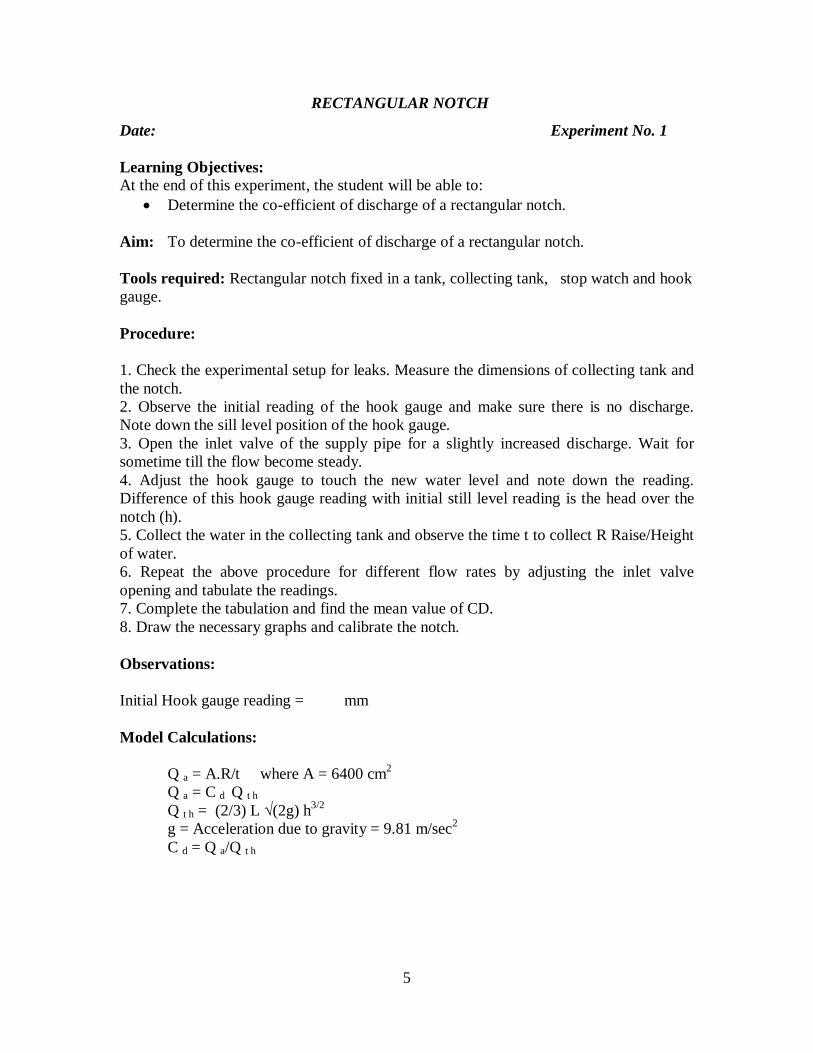
RECTANGULAR NOTCH

Date: Experiment No. 1 Learning Objectives: At the end of this experiment, the student will be able to:

Determine the co-efficient of discharge of a rectangular notch.

Aim: To determine the co-efficient of discharge of a rectangular notch. Tools required: Rectangular notch fixed in a tank, collecting tank, stop watch and hook gauge. Procedure: 1. Check the experimental setup for leaks. Measure the dimensions of collecting tank and the notch. 2. Observe the initial reading of the hook gauge and make sure there is no discharge. Note down the sill level position of the hook gauge. 3. Open the inlet valve of the supply pipe for a slightly increased discharge. Wait for sometime till the flow become steady. 4. Adjust the hook gauge to touch the new water level and note down the reading. Difference of this hook gauge reading with initial still level reading is the head over the notch (h). 5. Collect the water in the collecting tank and observe the time t to collect R Raise/Height of water. 6. Repeat the above procedure for different flow rates by adjusting the inlet valve opening and tabulate the readings. 7. Complete the tabulation and find the mean value of CD. 8. Draw the necessary graphs and calibrate the notch. Observations: Initial Hook gauge reading = mm Model Calculations:

Q a = A.R/t where A = 6400 cm2 Q a = C d Q t h Q t h = (2/3) L √(2g) h3/2 g = Acceleration due to gravity = 9.81 m/sec2 C d = Q a/Q t h

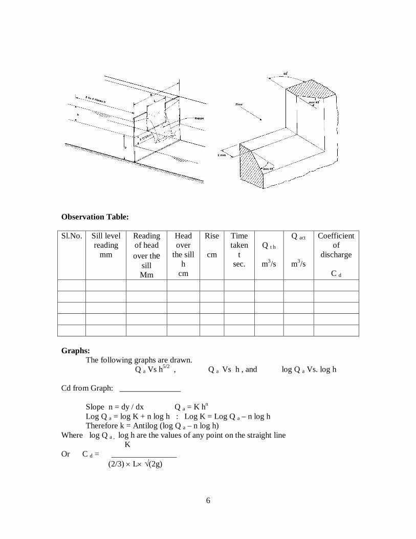
6

Observation Table: Sl.No. Sill level

reading mm

Reading of head over the

sill Mm

Head over

the sill h

cm

Rise

cm

Time taken

t sec.

Q t h

m3/s

Q act

m3/s

Coefficient of

discharge

C d Graphs:

The following graphs are drawn. Q a Vs h5/2 , Q a Vs h , and log Q a Vs. log h Cd from Graph: _______________

Slope n = dy / dx Q a = K hn Log Q a = log K + n log h : Log K = Log Q a – n log h Therefore k = Antilog (log Q a – n log h)

Where log Q a , log h are the values of any point on the straight line K Or C d = ________________ (2/3) L √(2g)

7

Result: Coefficient of discharge of the given triangular notch from

1. Observations ___________ 2. Graph ___________

Review Questions:

1. Comment on the location of pointer gauge

2. What is a broad crested weir? Bring out the points of difference vis-à-vis or sharp

crested weir

3. What are the advantages of a triangular notch or weir over a rectangular notch?

4. What is the effect on computed discharge over a weir or notch due to error in the

measurement of head?

5. How is discharge affected by the followings:

(a) Submerged weirs, and (b) Spillway and Siphon Spillway

6. What do you mean by a PROPORTIONAL or SUTRO weir? Is it possible to

design a weir of such a shape for which Q x H, i.e., discharge Q varies linearly

with the head H over the weir crest?

7. What is special about CIPOLLETTI weir (or Notch)?

8

TRIANGULAR NOTCH

Date: Experiment No.2 Learning Objectives: At the end of this experiment, the student will be able to:

Determine the co-efficient of discharge of a triangular notch. Aim: To determine the co-efficient of discharge of a triangular notch Tools required: Triangular Notch fixed to channel, collecting tank, stop watch, pointer gauge. Procedure: 1. Check the experimental setup for leaks. Measure the dimensions of collecting tank and the notch. 2. Observe the initial reading of the hook gauge and make sure there is no discharge. Note down the sill level position of the hook gauge. 3. Open the inlet valve of the supply pipe for a slightly increased discharge. Wait for sometime till the flow become steady. 4. Adjust the hook gauge to touch the new water level and note down the reading. Difference of this hook gauge reading with initial still level reading is the head over the notch (h). 5. Collect the water in the collecting tank and observe the time t to collect H Raise/Height of water. 6. Repeat the above procedure for different flow rates by adjusting the inlet valve opening and tabulate the readings. 7. Complete the tabulation and find the mean value of CD. 8. Draw the necessary graphs and calibrate the notch.

.

9

Observations: Initial Hook gauge reading = mm Model Calculations:

Q a = C d . Q t h Q a = A. H /t A = Area of collecting tank in Sq. cm

H = Rise of water in collecting tank in cm

T = Time taken for H cm rise of water in sec.

Q t h = (8/15) √(2g). Tan (θ/2). h5/2

Where g = Acceleration due to gravity cm/sec2

h = Head of water causing flow in cm

θ = Apex angle = 60o

C d = Q a/Q t h

10

Observation Table:

Sl. No.

Sill level

reading Mm

Reading of head over the sill mm

Head over

the sill h

cm

Rise

(cm)

Time taken

(t) (sec)

Q t h

(m3/s)

Q a ct

(m3/s)

Coefficient of discharge

C d

Graphs:

The following graphs are drawn. Q a Vs h5/2 ,

Q a Vs h , and

log Q a Vs. log h

Cd from Graph: Slope n = dy / dx

Q a = K hn

Log Q a = log K + n log h

Log K = Log Q a – n log h

Therefore k = Antilog (log Q a – n log h)

Q t h = (8/15) √2g. Tan (θ/2) h5/2

Therefore K = (8/15) C d √2g. Tanθ/2

K Or C d = ________________ (8/15) √2g. Tan (θ/2)

Result: Coefficient of discharge of the given triangular notch from

1. observations

2. graph

11

Review Questions:

1. Why should the geometrical shape of a notch be well defined and regular

2. What is meant by end contractions? Do they occur in all types of notches?

3. Comment on the form of calibration curve.

4. Is the value of Cd universal? If not, what factors may it depend upon?

5. Explain the terms “suppressed weir” and ‘Ventilation” of the nape.

12

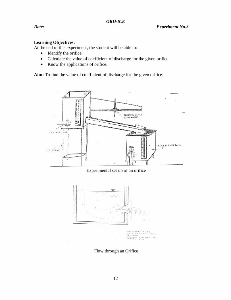
ORIFICE Date: Experiment No.3

Learning Objectives: At the end of this experiment, the student will be able to:

Identify the orifice. Calculate the value of coefficient of discharge for the given orifice Know the applications of orifice.

Aim: To find the value of coefficient of discharge for the given orifice.

Experimental set up of an orifice

Flow through an Orifice

13

Tools required: Stop watch and measuring scale etc. Procedure:

1. Fit the given orifice to the supply tank. 2. Note down the dimensions of the supply and measuring tanks using a scale. 3. Measure the diameter of the given orifice using vernier calipers. 4. Open the regulating valve fitted to the supply pipe and adjust it to maintain a

constant head in the tank. 5. Note down the time taken for a rise of 0.1 m of water level in the measuring tank. 6. Repeat the procedure for different heads

Observations:

1. Size of the supply tank = (l s b s h s) = -------------- m3 2. Size of the measuring tank = (l m b m h m) = ------------- m3 3. Diameter of the orifice (d) = ------------- m

Model Calculations: A R

1. Actual discharge (Q act) = ------ t

Where A = Cross-sectional area of measuring tank = (l m b m) = ------- m2

R= Rise of water column in measuring tank = --------- m

t = Time taken for ‘R’ units rise of water column in measuring tank = ------- sec

Therefore Q act = -------------- m3/s

2. Theoretical discharge (Q t h) = a o √(2gh)

Where

a o = Cross-sectional area of the orifice = (/4)d2 = --------- m2

h = Constant head in the supply tank = ------------- m Therefore Q t h = -------------- m3/s

3. Coefficient of discharge C d = Q act/Q t h = ------------.

14

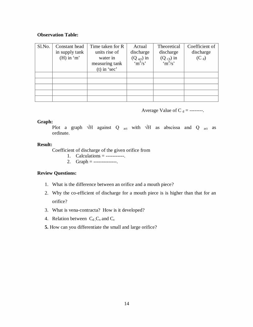
Observation Table: Sl.No. Constant head

in supply tank (H) in ‘m’

Time taken for R units rise of

water in measuring tank

(t) in ‘sec’

Actual discharge (Q act) in

‘m3/s’

Theoretical discharge (Q t h) in ‘m3/s’


(C d)

Average Value of C d = --------. Graph:

Plot a graph √H against Q act with √H as abscissa and Q act as ordinate.

Result:

Coefficient of discharge of the given orifice from 1. Calculations = -----------. 2. Graph = --------------.

Review Questions:

1. What is the difference between an orifice and a mouth piece?

2. Why the co-efficient of discharge for a mouth piece is is higher than that for an

orifice?

3. What is vena-contracta? How is it developed?

4. Relation between Cd ,Cv and Cc

5. How can you differentiate the small and large orifice?

15

MOUTHPIECE Date: Experiment No.4


Identify the Mouthpiece. Calculate the value of coefficient of discharge for the given mouthpiece. Know the applications of mouthpiece.

Aim: To find the value of coefficient of discharge for the given mouth piece. Model:

Experimental set up of Mouthpiece

16

Flow through an external cylindrical Mouthpiece Tools required: Stop watch and measuring scale etc. Procedure:

1. Fit the given mouth piece to the supply tank. 2. Note down the dimension of the supply tank using a scale. 3. Measure the dimensions of the given mouth piece using vernier calipers 4. Open the regulating valve fitted to the supply pipe and close it when the supply

tank is full of water. 5. Note down the time taken for the water level to fall through the head say ‘x’ units,

i.e., from an initial head H1 to final head H2 units. 6. Repeat the steps (4) and (5) for different values of H1 and H2 for the same range

‘x’. The following combination may be used, choosing x = 0.3 m.

H1 (m) To H2 (m) 0.80 To 0.50 0.75 To 0.45 0.70 To 0.40 0.65 To 0.35 0.60 To 0.30

Observations:

1. Size of the supply tank = (l s b s h s) = -------------- m3 2. Diameter of the mouthpiece (d) = ------------- m

Model Calculations: 2A [√H1 – √H2]

1. Coefficient of discharge (C d) = -------------------- t a √(2g)

Where A = Cross-sectional area of supply tank (ls x bs) = ------------ m2

H1 = Initial head in the supply tank above the center of mouth piece = --------- m H2 = Final head in the supply tank above the center of mouth piece = --------- m t = Time taken for water level to fall from H1 to H2 = ---------- sec g = Acceleration due to gravity = 9.81 m/s2

a = Cross-sectional area of the given mouth piece = (/4)d2 = ----- m2 Therefore C d = ----------------.

17

Observation Table:

Sl. No.

Initial head in the supply tank

H1 (m)

Final head in the supply tank H2 (m)

Time (t) taken for water level to fall from H1 to

H2

(sec)


C d

Average Value of C d = --------. Graph:

Plot a graph of [√H1 – √ H2] against time‘t’ with [√H1 – √H2] as abscissa and‘t’ as ordinate. Using the graph, find the coefficient of discharge.

Graphical Table: Sl.No. H1

(m) H2 (m)

[√H1 –√ H2] (m)

T (sec)

Result:

Coefficient of discharge of the given orifice from 1. Calculations = -----------. 2. Graph = --------------.

Review Questions:

1. What is so special about Borda’s mouth piece? 2. What are the various types of mouth pieces? 3. What is the difference between an orifice and a mouth piece? 4. Why the co-efficient of discharge for a mouth piece is higher than that for an

orifice? 5. Cc for the mouth piece is equal to 1 why? 6. Cd for an external cylindrical mouth piece is more that for a standard orifice of the

same diameter and under the same head, why? 7. Under what condition a mouth piece behaves as an orifice? Under what condition

of discharge the external cylindrical mouthpiece is said to be running free?

18

ORIFICE-METER Date: Experiment No.5


Identify the Orifice meter. Calculate the value of coefficient of discharge for the given orifice meter. Know the applications of orifice meter.

Aim: To determine the coefficient of discharge of a given Orifice-meter. Model:

Fig.. Orifice Meter

Tools required: Stop watch and measuring scale etc. Procedure: 1. Check the experimental setup for leaks. Measure the dimensions of collecting tank. Note down the flow meter specifications. 2. Open the inlet valve fully and allow the water to fill fully in the flow meter. 3. Make sure the height of Mercury column in both limbs are same if there is no

Discharge through the meter. 4. Slightly open the outlet valve of the flow meter and observe the manometer limbs. 5. Adjust it to get a steady pressure difference between the limbs of the manometer. Note down the corresponding Mercury levels.

19

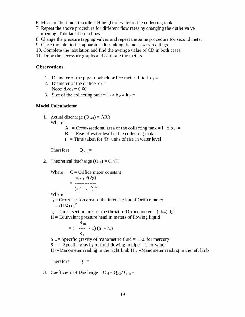
6. Measure the time t to collect H height of water in the collecting tank. 7. Repeat the above procedure for different flow rates by changing the outlet valve opening. Tabulate the readings. 8. Change the pressure tapping valves and repeat the same procedure for second meter. 9. Close the inlet to the apparatus after taking the necessary readings. 10. Complete the tabulation and find the average value of CD in both cases. 11. Draw the necessary graphs and calibrate the meters. Observations:

1. Diameter of the pipe to which orifice meter fitted d1 = 2. Diameter of the orifice, d2 =

Note: d2/d1 = 0.60. 3. Size of the collecting tank = l c b c h c =

Model Calculations:

1. Actual discharge (Q act) = AR/t Where

A = Cross-sectional area of the collecting tank = l c x b c = R = Rise of water level in the collecting tank = t = Time taken for ‘R’ units of rise in water level

Therefore Q act =

2. Theoretical discharge (Qt h) = C √H

Where C = Orifice meter constant

a1 a2 √(2g) = ------------- (a1

2 – a22)1/2

Where a1 = Cross-section area of the inlet section of Orifice meter = (/4) d1

2

a2 = Cross-section area of the throat of Orifice meter = (/4) d22

H = Equivalent pressure head in meters of flowing liquid S m = ( ---- - 1) (h1 – h2) S f

S m = Specific gravity of manometric fluid = 13.6 for mercury S f = Specific gravity of fluid flowing in pipe = 1 for water H 1=Manometer reading in the right limb,H 2 =Manometer reading in the left limb

Therefore Qth =

3. Coefficient of Discharge C d = Qact / Qt h =

20

Observation Table:

S. No Manometric reading

Time taken for ‘R’ units rise of

water level (t) in ‘sec’

Actual discharge

(Q act) in

‘m3/s’

Theoretical discharge

(Q t h) in

‘m3/s’

Coefficient of

discharge (C d)

Right limb

(h1) in ‘m’

Left limb

(h2) in ‘m’

Average Value of C d = --------.

Graph: Plot a graph of √H against actual discharge taking √H on the abscissa and Q act on the ordinate. Using the graph, find the coefficient of discharge. Graphical Table:

Result:

Coefficient of discharge of the given orifice meter from 1. Calculations = -----------. 2. Graph = --------------.

Review Questions:

1. Why contraction occurs? 2. Why there is difference between the theoretical and the actual velocity of the jet at vena-contracta? 3. What do you mean by the term ‘coefficient of resistance’? How can it be determined by knowing the value of CV of the orifice? 4. For a large vertical orifice, can the discharge be computed by the same equation

as that for a small orifice? 5. When should an orifice be treated as a small orifice? 6. The coefficient of discharge for an orifice meter is much smaller than that for a

venturimeter, why?

Sl.No. h1 (m) h2 (m) H (m) √ H (m)

Q act (m3/s)

21

VENTURIMETER

Date: Experiment No.6


Identify the venturimeter. Calculate the value of coefficient of discharge for the given venturimeter. Know the applications of venturimeter.

Aim: To determine the coefficient of discharge for a given Venturimeter. Model:

Fig.. Venturimeter


1. Select the desired Venturimeter whose coefficient of discharge is to be determined.

2. Connect the pressure tapings of the Venturimeter selected to the Piezometric tubes of the Manometer provided.

3. Open the regulating valve so that water starts flowing through the Venturimeter. Wait for sometime so that the flow gets stabilized.

4. Vent the manometer, if necessary. 5. Note down differential Manometer readings h1 and h2 6. Measure the actual discharge by observing the time taken to collect a

predetermined volume of water. (Time taken for 10 cm rise of water column in the collecting tank may be noted and actual discharge found).

7. Repeat steps (5) and (6) for different flow rates (by adjusting regulating valve) and take at least six different sets of observations.

22

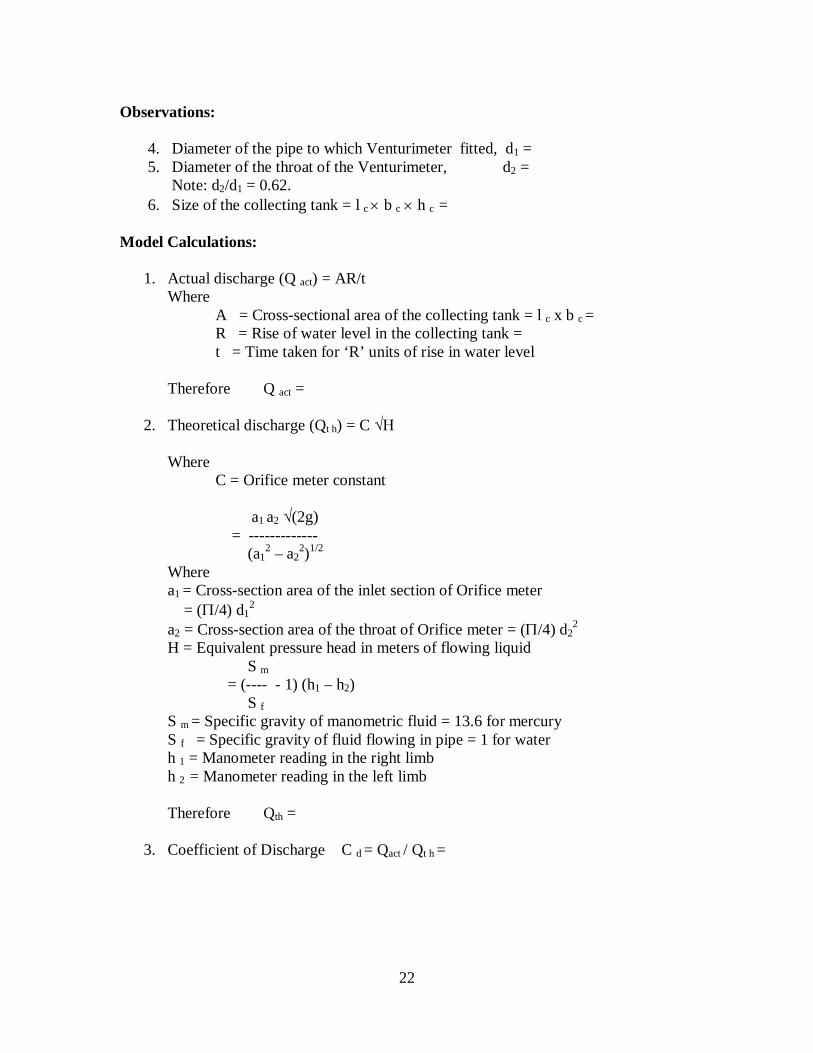
Observations:

4. Diameter of the pipe to which Venturimeter fitted, d1 = 5. Diameter of the throat of the Venturimeter, d2 =

Note: d2/d1 = 0.62. 6. Size of the collecting tank = l c b c h c =

Model Calculations:

1. Actual discharge (Q act) = AR/t Where

A = Cross-sectional area of the collecting tank = l c x b c = R = Rise of water level in the collecting tank = t = Time taken for ‘R’ units of rise in water level

Therefore Q act =

2. Theoretical discharge (Qt h) = C √H

Where

C = Orifice meter constant a1 a2 √(2g) = ------------- (a1

2 – a22)1/2

Where a1 = Cross-section area of the inlet section of Orifice meter = (/4) d1

2

a2 = Cross-section area of the throat of Orifice meter = (/4) d22

H = Equivalent pressure head in meters of flowing liquid S m = (---- - 1) (h1 – h2) S f

S m = Specific gravity of manometric fluid = 13.6 for mercury S f = Specific gravity of fluid flowing in pipe = 1 for water h 1 = Manometer reading in the right limb h 2 = Manometer reading in the left limb

Therefore Qth =

3. Coefficient of Discharge C d = Qact / Qt h =

23

Observation Table:

S. No Manometric reading

Time taken for ‘R’ units rise of

water level (t) in ‘sec’

Actual discharge

(Q act) in

‘m3/s’

Theoretical discharge

(Q t h) in

‘m3/s’

Coefficient of

discharge (C d)

Right limb

(h1) in ‘m’

Left limb

(h2) in ‘m’

Average Value of C d = --------.

Graph: Plot a graph of √H against actual discharge taking √H on the abscissa and Q act on the ordinate. Using the graph, find the coefficient of discharge. Graphical Table:

Result:

Coefficient of discharge of the Venturimeter from 1. Calculations = -----------. 2. Graph = --------------.

Review Questions:

1. The meter discharge coefficient Cd is less than unity if the pressure head h is measured across the converging piece. The value of Cd will be greater than one if the measurements are taken across the diverging piece of venturimeter.

2. Can be the same calibration be used if the venturimeter is inclined? 3. Comment and discuss on the usefulness of this experiment based on the plots

prepared 4. How discharge coefficient varies as the area ratio is changed and with change in

manometer reading? 5. What are the relative advantages and limitations of a venturimeter versus other

flow meters?

Sl.No. h1 (m) h2 (m) H (m) √ H

Q act (m3/s)

24

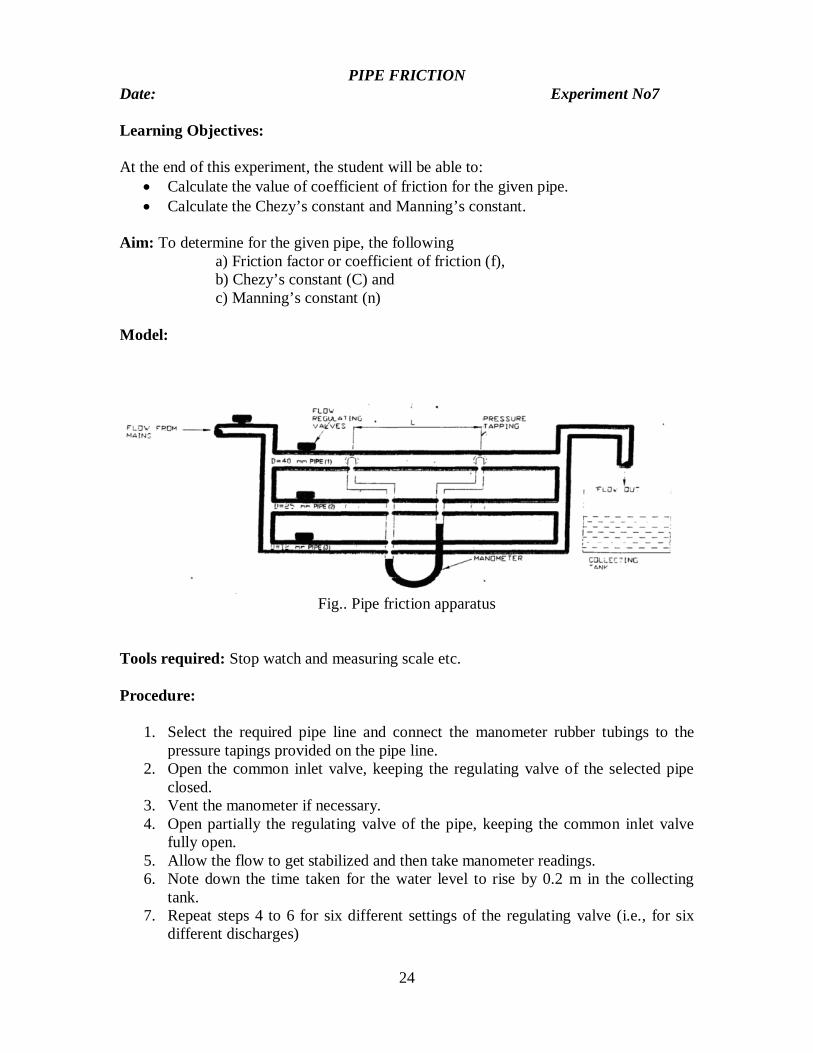
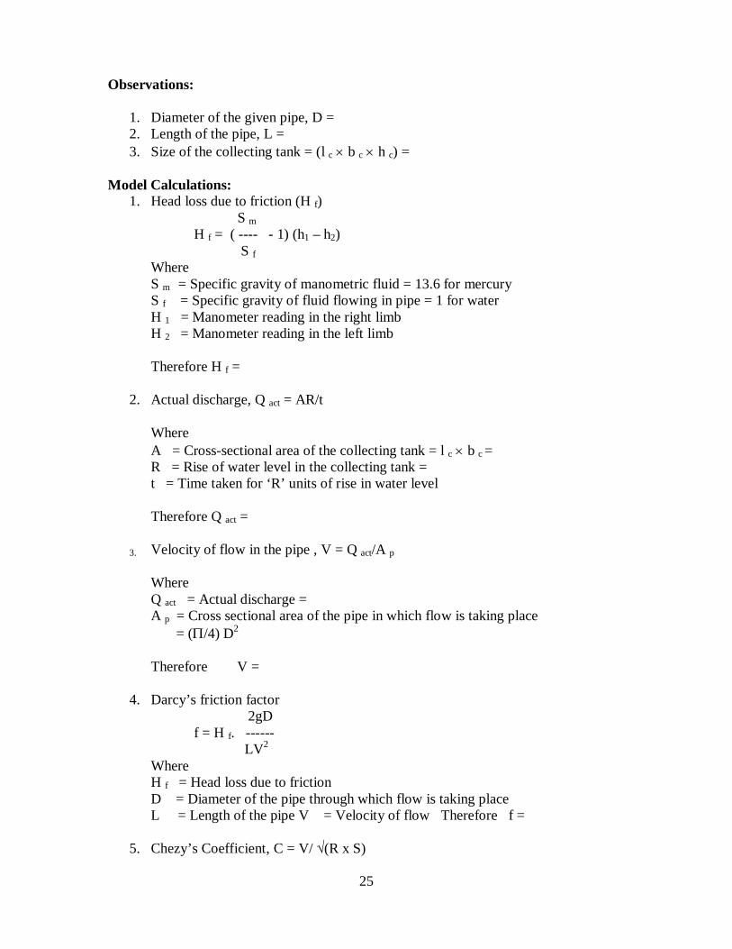
PIPE FRICTION Date: Experiment No7


Calculate the value of coefficient of friction for the given pipe. Calculate the Chezy’s constant and Manning’s constant.

Aim: To determine for the given pipe, the following

a) Friction factor or coefficient of friction (f), b) Chezy’s constant (C) and c) Manning’s constant (n)

Model:

Fig.. Pipe friction apparatus


1. Select the required pipe line and connect the manometer rubber tubings to the pressure tapings provided on the pipe line.

2. Open the common inlet valve, keeping the regulating valve of the selected pipe closed.

3. Vent the manometer if necessary. 4. Open partially the regulating valve of the pipe, keeping the common inlet valve

fully open. 5. Allow the flow to get stabilized and then take manometer readings. 6. Note down the time taken for the water level to rise by 0.2 m in the collecting

tank. 7. Repeat steps 4 to 6 for six different settings of the regulating valve (i.e., for six

different discharges)

25

Observations:

1. Diameter of the given pipe, D = 2. Length of the pipe, L = 3. Size of the collecting tank = (l c b c h c) =

Model Calculations:

1. Head loss due to friction (H f) S m H f = ( ---- - 1) (h1 – h2) S f

Where S m = Specific gravity of manometric fluid = 13.6 for mercury S f = Specific gravity of fluid flowing in pipe = 1 for water H 1 = Manometer reading in the right limb H 2 = Manometer reading in the left limb

Therefore H f =

2. Actual discharge, Q act = AR/t

Where A = Cross-sectional area of the collecting tank = l c b c = R = Rise of water level in the collecting tank = t = Time taken for ‘R’ units of rise in water level

Therefore Q act =

3. Velocity of flow in the pipe , V = Q act/A p

Where Q act = Actual discharge = A p = Cross sectional area of the pipe in which flow is taking place = (/4) D2

Therefore V =

4. Darcy’s friction factor

2gD f = H f. ------ LV2

Where H f = Head loss due to friction D = Diameter of the pipe through which flow is taking place L = Length of the pipe V = Velocity of flow Therefore f =

5. Chezy’s Coefficient, C = V/ √(R x S)

26

Where V = Velocity of flow = R = Hydraulic radius = D/4 = S = Slope of hydraulic gradient = H f/L = Therefore C =

6. Manning’s Roughness Coefficient (n):

R2/3 . S1/2 n = ----------- V

Where R = Hydraulic radius = S = Slope of hydraulic gradient = V = Velocity of flow = Therefore n =

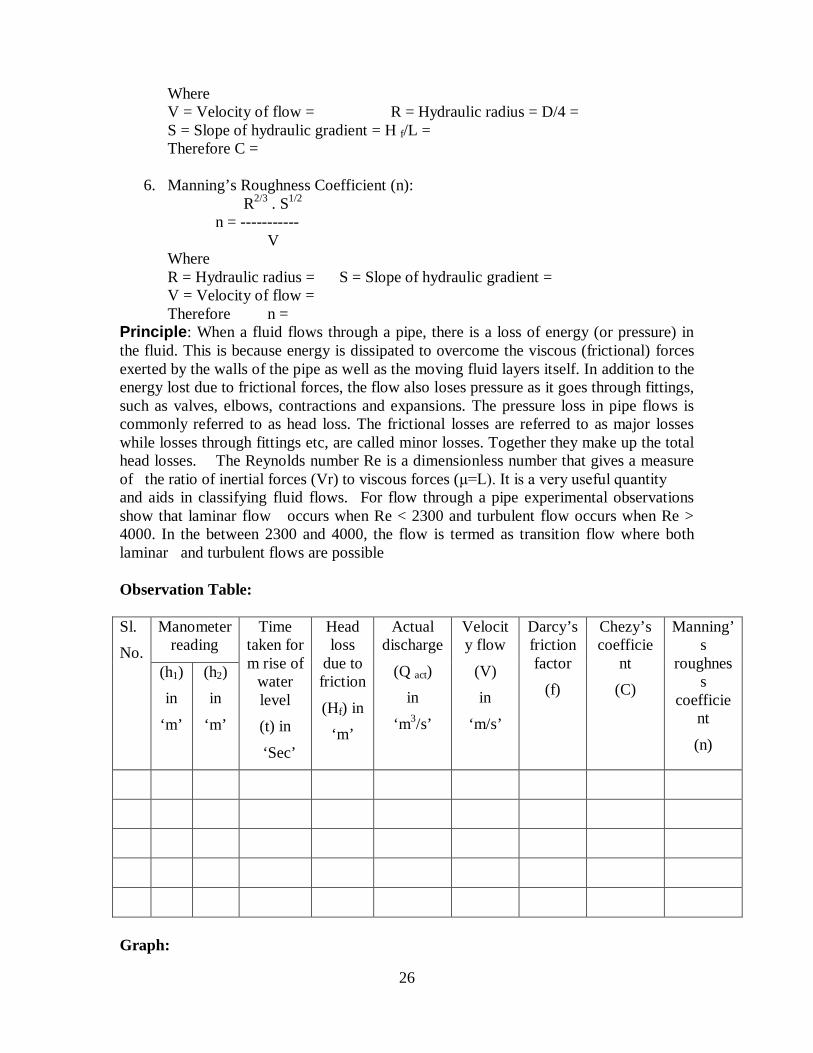
Principle: When a fluid flows through a pipe, there is a loss of energy (or pressure) in the fluid. This is because energy is dissipated to overcome the viscous (frictional) forces exerted by the walls of the pipe as well as the moving fluid layers itself. In addition to the energy lost due to frictional forces, the flow also loses pressure as it goes through fittings, such as valves, elbows, contractions and expansions. The pressure loss in pipe flows is commonly referred to as head loss. The frictional losses are referred to as major losses while losses through fittings etc, are called minor losses. Together they make up the total head losses. The Reynolds number Re is a dimensionless number that gives a measure of the ratio of inertial forces (Vr) to viscous forces (μ=L). It is a very useful quantity and aids in classifying fluid flows. For flow through a pipe experimental observations show that laminar flow occurs when Re < 2300 and turbulent flow occurs when Re > 4000. In the between 2300 and 4000, the flow is termed as transition flow where both laminar and turbulent flows are possible Observation Table: Sl. No.

Manometer reading

Time taken for m rise of

water level (t) in

‘Sec’

Head loss

due to friction

(Hf) in ‘m’

Actual discharge

(Q act) in

‘m3/s’

Velocity flow

(V) in

‘m/s’

Darcy’s friction factor

(f)

Chezy’s coefficie

nt (C)

Manning’s

roughness

coefficient

(n)

(h1) in

‘m’

(h2) in

‘m’

Graph:

27

Plot a graph of log V against log H f taking log H f on the abscissa and log V as ordinate. Using the graph, find the value of the Darcy’s friction factor f. Graphical Table:

S.No. H f Log H f V Log V

Result:

1. The value of Darcy’s friction factor from a) calculations = b) graph =

2. The value of Chezy’s coefficient = 3. The value of Manning’s roughness coefficient =

Review Questions:

1. List different types of pipe flows?

2. Indicate the type and magnitude of possible errors occurring in this test.

3. Deduce the effect of the pipe diameter on friction coefficient of a pipe.

4. Discuss Moody’s diagram.

5. Show that, for a laminar flow f = 64/Re. How do the results for laminar flow

compare with this equation and with Blasius equation?

6. What is the significance of upper and lower Reynolds number and what are

their values?

7. What is the effect of ageing of a pipe line on the friction factor aged pipe line?

28

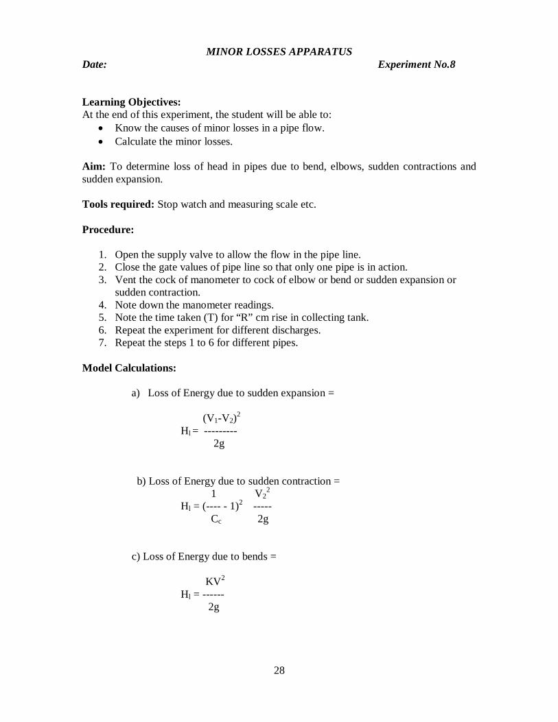
MINOR LOSSES APPARATUS Date: Experiment No.8 Learning Objectives: At the end of this experiment, the student will be able to:

Know the causes of minor losses in a pipe flow. Calculate the minor losses.

Aim: To determine loss of head in pipes due to bend, elbows, sudden contractions and sudden expansion. Tools required: Stop watch and measuring scale etc. Procedure:

1. Open the supply valve to allow the flow in the pipe line. 2. Close the gate values of pipe line so that only one pipe is in action. 3. Vent the cock of manometer to cock of elbow or bend or sudden expansion or

sudden contraction. 4. Note down the manometer readings. 5. Note the time taken (T) for “R” cm rise in collecting tank. 6. Repeat the experiment for different discharges. 7. Repeat the steps 1 to 6 for different pipes.

Model Calculations:

a) Loss of Energy due to sudden expansion =

(V1-V2)2 Hl = ---------

2g b) Loss of Energy due to sudden contraction = 1 V2

2 Hl = (---- - 1)2 -----

Cc 2g c) Loss of Energy due to bends =

KV2 Hl = ------

2g

29

Observation Table

Result: Head loss due to sudden expansion =

Head loss due to sudden contraction =

Head loss due to elbow & bends =

Review Questions:

1. What are the minor losses? Under what circumstances will they be negligible?

2. What is entrance loss? Give the approximate values of loss coefficient for

different types of pipe entrances?

3. What are the causes of loss of energy in pipe bends?

4. What are the effects of formation of vena-contracts at the entrance to a pipe?

How it can be accounted for?

5. What do you mean by ‘WATER HAMMER’ in pipes? Hence deduce the effect

of gradual and instantaneous closure of a valve.

30

BERNOULLI’S EQUATION Date: Experiment No.9

Learning Objectives: At the end of this experiment, the student will be able to

Know the Bernoulli’s principle. Applications of Bernoulli’s principle.

Aim: To verify the Bernoulli’s equation experimentally. Model:

Fig.. Bernoulli’s Apparatus


1. Note down the area of cross section of the conduit at various piezometer points.

31

2. Open the supply valve and adjust the flow so that the water level in the inlet tank remains at a constant level (i.e., flow becomes steady).

3. Measure the height of water level in different Piezometers. 4. Measure the discharge. 5. Repeat setups 2 to 4 for two more readings.

Observation Table

Trail Run

Head Maintained in Supply Tank (m)

Time for 20 cm rise

(sec)

Discharge Q

m3/sec

Piezometer Distance from a reference point

1 2 3 4 5 6 7 8 9 10 11 12 13

Run 1

Velocity, V=Q/A V2/2g

(P/γ)+Z E=(P/γ)+Z+(V2/2g)

Run 2


(P/γ)+Z E=(P/γ)+Z+(V2/2g)

Run 3


(P/γ)+Z E=(P/γ)+Z+(V2/2g)

Graphs:

1. Plot (P/γ) + Z Vs distance of Piezometer tubes for some reference ( on x-axis). Join the points by a smooth curve. This is known as the hydraulic line.

2. E = (P/γ) + Z + (V2/2g) Vs distance of piezometer tubes. Join the points

smoothly. This is the total energy line. Result: Total energy line remains the same at different sections. Review Questions:

1. Each term in the Bernoulli’s equation represents_______________________. 2. Is constant in Bernoulli’s equation same for all kinds of flow streamline flow

potential. If so, why? If not, Why? 3. Write Bernoulli’s equation for real fluid flow. 4. What are the assumptions made in Bernoulli’s equation’s derivation? 5. What are the applications of Bernoulli’s equation?

32

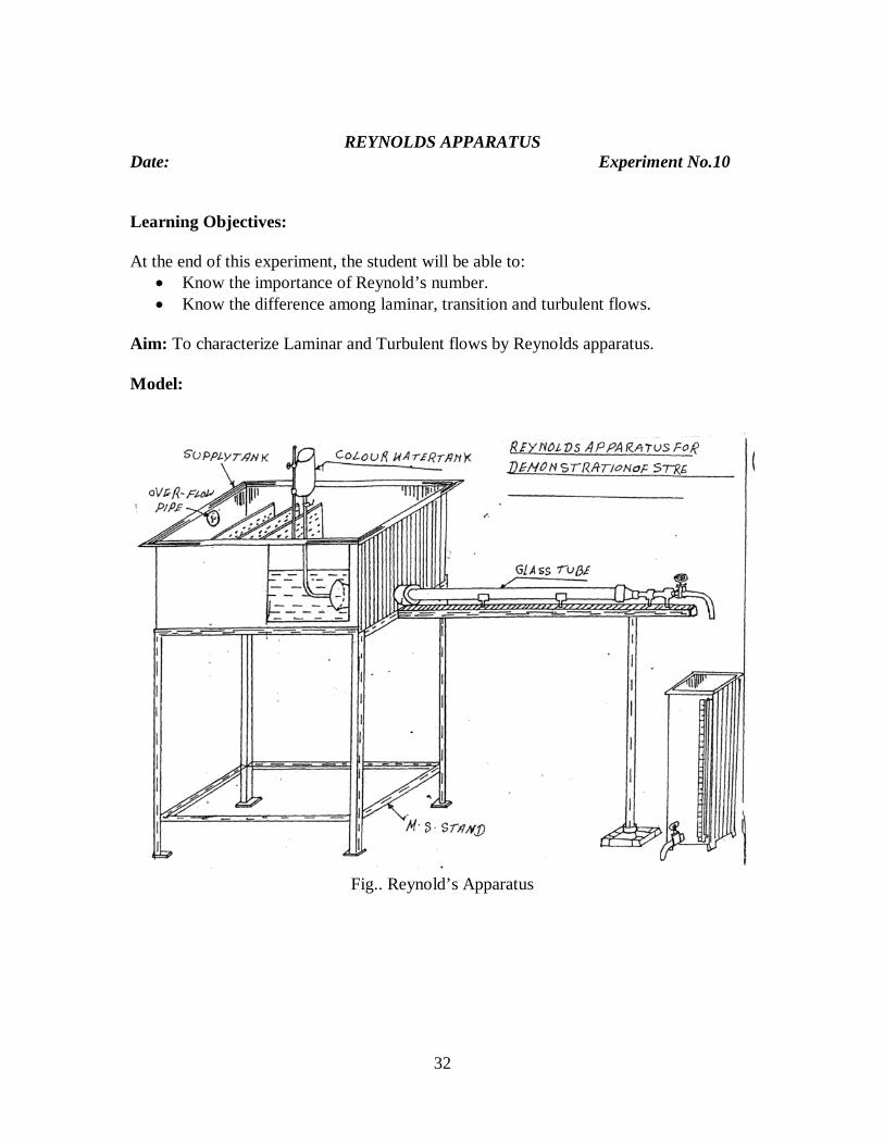
REYNOLDS APPARATUS Date: Experiment No.10 Learning Objectives: At the end of this experiment, the student will be able to:

Know the importance of Reynold’s number. Know the difference among laminar, transition and turbulent flows.

Aim: To characterize Laminar and Turbulent flows by Reynolds apparatus. Model:

Fig.. Reynold’s Apparatus

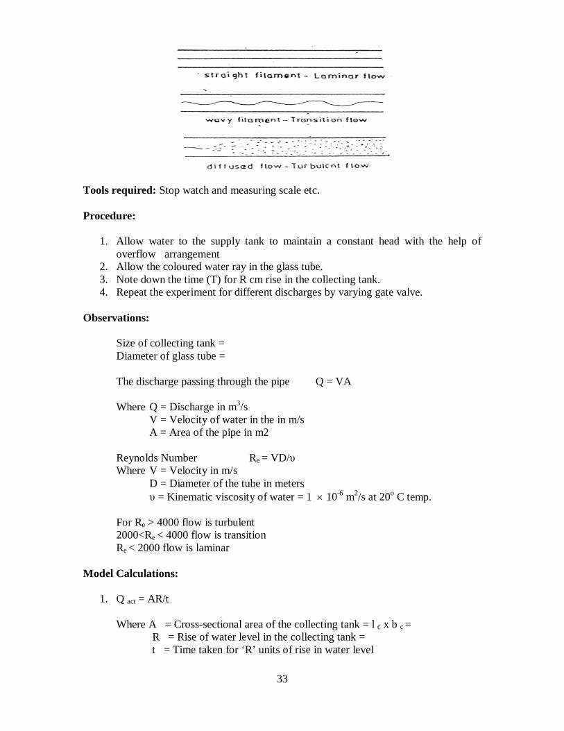
33


1. Allow water to the supply tank to maintain a constant head with the help of overflow arrangement

2. Allow the coloured water ray in the glass tube. 3. Note down the time (T) for R cm rise in the collecting tank. 4. Repeat the experiment for different discharges by varying gate valve.

Observations:

Size of collecting tank =

Diameter of glass tube = The discharge passing through the pipe Q = VA

Where Q = Discharge in m3/s V = Velocity of water in the in m/s A = Area of the pipe in m2

Reynolds Number Re = VD/υ Where V = Velocity in m/s

D = Diameter of the tube in meters υ = Kinematic viscosity of water = 1 10-6 m2/s at 20o C temp.

For Re > 4000 flow is turbulent 2000<Re < 4000 flow is transition Re < 2000 flow is laminar

Model Calculations:

1. Q act = AR/t

Where A = Cross-sectional area of the collecting tank = l c x b c = R = Rise of water level in the collecting tank = t = Time taken for ‘R’ units of rise in water level

34

Therefore Q act = 2. Reynolds Number R e = VD/υ

Where V = Velocity in m/s

D = Diameter of the tube in meters υ = Kinematic viscosity of water = 1 x 10-6 m2/s at 20oC temp.

Therefore Re =

3. Type of flow: Observation Table Sl.No. Time taken for

R cm rise T sec.

Discharge Q = AR/t

m3/s

Velocity (V) in glass tube

(m/s)

Reynolds’s number

Re = VD/υ

Type of flow

Result: Review Questions:

1. How do you distinguish physically a laminar flow and turbulent flow?

2. What is Reynolds number?

3. How does Reynolds number helps in distinguish the nature of flow?

4. What is critical Reynolds number for a pipe flow

5. Under what circumstances the flow is expected to be laminar

6. What are responsible parameters flow to be turbulent?

7. What is effect of Reynolds number on friction factor?

8. What are basic equations required in the derivation of Darcy whish back

equation?

9. What do you mean by fully developed flow?

35

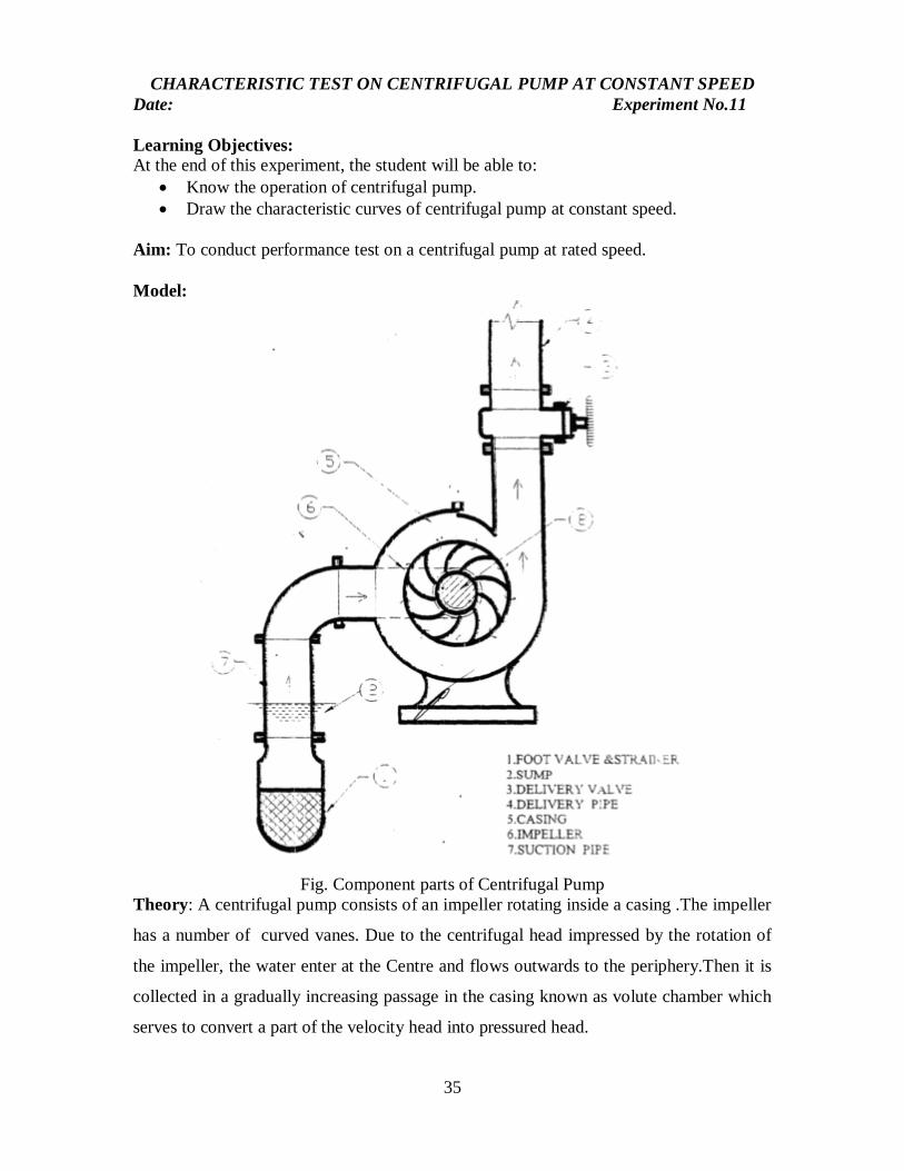
CHARACTERISTIC TEST ON CENTRIFUGAL PUMP AT CONSTANT SPEED Date: Experiment No.11 Learning Objectives: At the end of this experiment, the student will be able to:

Know the operation of centrifugal pump. Draw the characteristic curves of centrifugal pump at constant speed.

Aim: To conduct performance test on a centrifugal pump at rated speed. Model:

Fig. Component parts of Centrifugal Pump

Theory: A centrifugal pump consists of an impeller rotating inside a casing .The impeller

has a number of curved vanes. Due to the centrifugal head impressed by the rotation of

the impeller, the water enter at the Centre and flows outwards to the periphery.Then it is

collected in a gradually increasing passage in the casing known as volute chamber which

serves to convert a part of the velocity head into pressured head.

36

For a higher heads multi stage centrifugal pumps having two or more impellers in series

will have to be used. This single stage centrifugal pump of size (50mm x 50mm) is

coupled to 3 HP capacity Squirrel cage induction motor. The suction side is 50mm dia

and delivery side is 50mm dia.An energy meter is provided to measure the input to the

motor and collecting tank to measure the discharge. A pressure gauge and vacuum gauge

are fitted in delivery and suction sides to measure the head of water. The pump must be

full of water upto delivery valve before starting. For this reason it should not be allowed

water to drain and hence a foot valve is provided. But after the long run the leather valve

in the

foot valve becomes useless and so the foot valve becomes leaky.In this case the pump

should be primed by pouring water.

Tools required: Stop watch, measuring scale and Energy meter etc. Procedure:

1. Check the pressure gauges. Make sure both of them show atmospheric pressure. 2. Observe the suction and delivery pipe diameters. Measure the dimensions of

collecting tank. Measure the difference in elevation between the suction and delivery pressure tapings.

3. Prime the centrifugal pump. Keep the delivery valve fully closed. 4. Start the pump. 5. Open the delivery valve slightly. Observe the pressure gauge readings. 6. Measure the discharge using the collecting tank stopwatch setup. 7. Note the time for n revolutions of the energy meter disk. 8. Open the delivery valve gradually to maximum. Repeat the above observations

for different discharges. 9. Tabulate the readings. Draw the performance characteristics; H Vs. Q, Pbhp 10. Vs. Q and h Vs. Q.

Observations:

1. Size of the collecting tank = l b h 2. Diameter of the suction pipe, ds = 50 mm 3. Diameter of the delivery pipe, dd = 50 mm 4. Energy meter constant, N = 400 rev / KWH 5. Difference in the levels of pressure and vacuum gauges,

X = 43cm. Model Calculations:

1. Actual discharge : Q = AR/t (m3/s)

37

Where A: Cross-sectional area of collecting tank = l b R: Rise of water column in collecting tank in meters t: Time taken for ‘R’ units rise of water column in seconds

Q = m3/s

2. Pressure gauge reading in metres of water column (Hg)

Hg = (Pg 104 9.81)/ 9810 m

Pg = Pressure gauge reading in kg/cm2

Hg =

3. Vacuum gauge reading in meters of water column (Hv)

Hv = (hv 10-3 x 13.6) m of water

Hv = Vacuum gauge reading

4. Velocity head in delivery pipe (Vd2 / 2g)

Vd : Velocity of flow in delivery pipe = Q/(/4 dd2)

(Vd2 / 2g) =

5. Velocity head in suction pipe (Vs2/ 2g)

Vs : Velocity of flow in suction pipe = Q/(/4ds2)

(V2s / 2g) =

6. Total head in the pump (H)

H : Hg + Hv + X

7. Output of the pump (O/P)

Out Put = .Q.H Watts

8. Input to the pump (I/P)

I/P = (3600 n) / (N T)

n : Number of revolutions of energy meter

N : Energy meter constant rev/ kWh

T : Time for ‘n’ revolutions of energy meter in sec.

38

9. Overall efficiency (o)

o = Output/Input

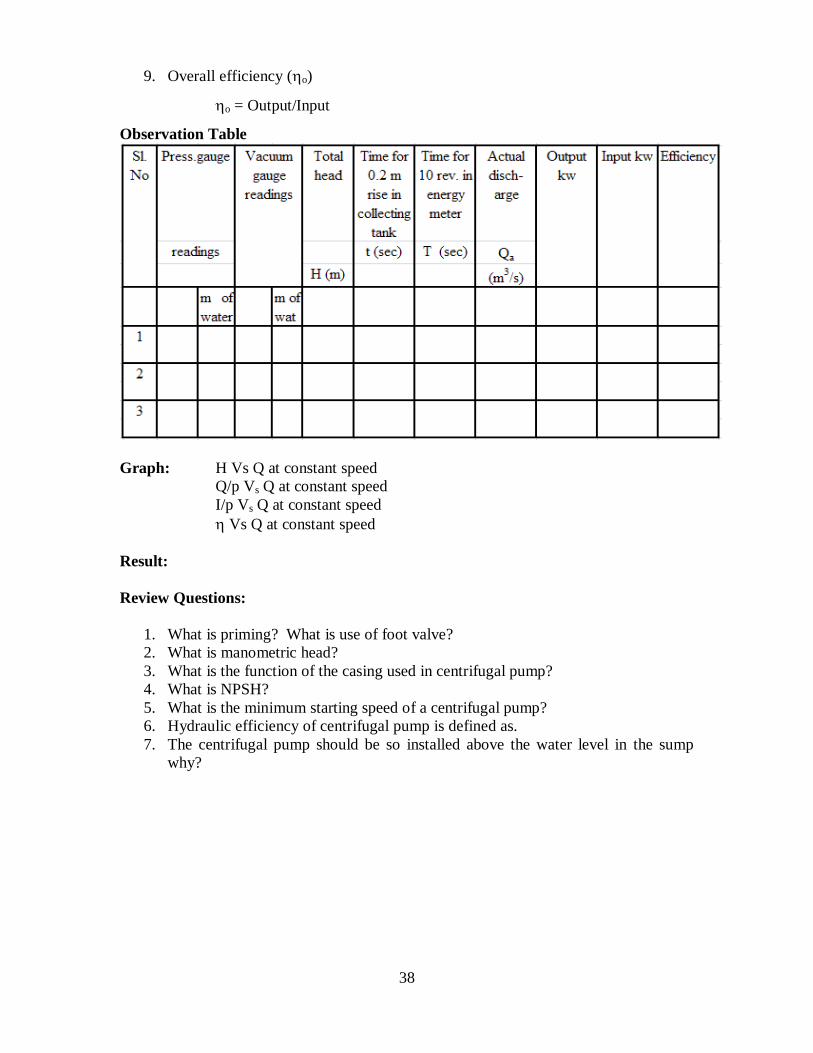
Observation Table

Graph: H Vs Q at constant speed Q/p Vs Q at constant speed I/p Vs Q at constant speed Vs Q at constant speed Result: Review Questions:

1. What is priming? What is use of foot valve? 2. What is manometric head? 3. What is the function of the casing used in centrifugal pump? 4. What is NPSH? 5. What is the minimum starting speed of a centrifugal pump? 6. Hydraulic efficiency of centrifugal pump is defined as. 7. The centrifugal pump should be so installed above the water level in the sump

why?

39

CHARACTERISTIC TEST ON CENTRIFUGAL PUMP SET AT RATED-SPEED


Know the operation of centrifugal pump. Draw the characteristic curves of centrifugal pump at constant speed.

Aim: To conduct performance test on a centrifugal pump at rated speed. Model:

Fig. Component parts of Centrifugal Pump

40

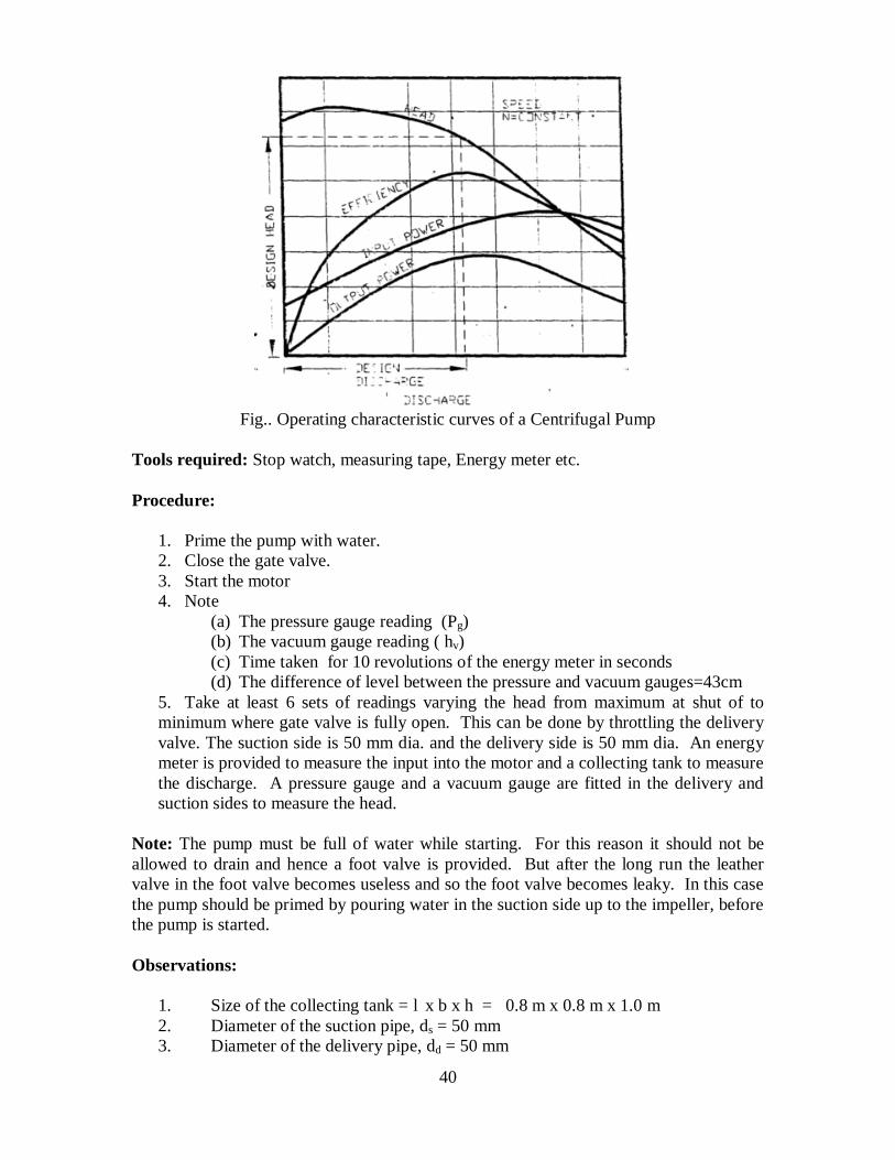
Fig.. Operating characteristic curves of a Centrifugal Pump

Tools required: Stop watch, measuring tape, Energy meter etc. Procedure:

1. Prime the pump with water. 2. Close the gate valve. 3. Start the motor 4. Note

(a) The pressure gauge reading (Pg) (b) The vacuum gauge reading ( hv) (c) Time taken for 10 revolutions of the energy meter in seconds (d) The difference of level between the pressure and vacuum gauges=43cm

5. Take at least 6 sets of readings varying the head from maximum at shut of to minimum where gate valve is fully open. This can be done by throttling the delivery valve. The suction side is 50 mm dia. and the delivery side is 50 mm dia. An energy meter is provided to measure the input into the motor and a collecting tank to measure the discharge. A pressure gauge and a vacuum gauge are fitted in the delivery and suction sides to measure the head.

Note: The pump must be full of water while starting. For this reason it should not be allowed to drain and hence a foot valve is provided. But after the long run the leather valve in the foot valve becomes useless and so the foot valve becomes leaky. In this case the pump should be primed by pouring water in the suction side up to the impeller, before the pump is started. Observations:

1. Size of the collecting tank = l x b x h = 0.8 m x 0.8 m x 1.0 m 2. Diameter of the suction pipe, ds = 50 mm 3. Diameter of the delivery pipe, dd = 50 mm

41

4. Energy meter constant, N = 400 rev/kwh 5. Difference in the levels of pressure and vacuum gauges,

X = 430 mm. Model Calculations: 1. Actual Discharge: (Q) Q = AR/t (m3/s)

Where A: Cross-sectional area of collecting tank = l b R: Rise of water column in collecting tank in meters t: Time taken for ‘R’ units rise of water column in seconds

Q = m3/s

2. Pressure gauge reading in metres of water column (Hg)

Hg = (Pg 104 9.81)/ 9810 m

Pg = Pressure gauge reading in kg/cm2

Hg =

2. Vacuum gauge reading in meters of water column (Hv)

Hv = (hv 10-3 x 13.6) m of water

Hv = Vacuum gauge reading

3. Velocity head in delivery pipe (Vd2 / 2g)

Vd : Velocity of flow in delivery pipe = Q/(/4 dd2)

(Vd2 / 2g) =

4. Velocity head in suction pipe (Vs2/ 2g)

Vs : Velocity of flow in suction pipe = Q/(/4ds2)

(V2s / 2g) =

5. Total head in the pump (H)

H : Hg + Hv + X

6. Output of the pump (O/P)

Out Put = .Q.H Watts

42

7. Input to the pump (I/P)

I/P = (3600 n) / (N T)

n : Number of revolutions of energy meter

N : Energy meter constant rev/ kWh

T : Time for ‘n’ revolutions of energy meter in sec.

8. Overall efficiency (o)

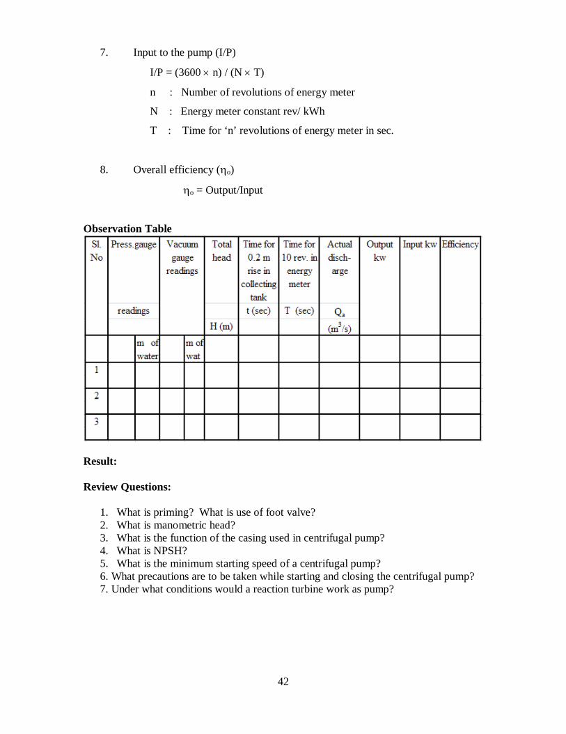
o = Output/Input Observation Table


1. What is priming? What is use of foot valve? 2. What is manometric head? 3. What is the function of the casing used in centrifugal pump? 4. What is NPSH? 5. What is the minimum starting speed of a centrifugal pump? 6. What precautions are to be taken while starting and closing the centrifugal pump? 7. Under what conditions would a reaction turbine work as pump?

43

RECIPROCATING PUMP (PLUNGER PUMP) Date: Experiment No.13 Learning Objectives: At the end of this experiment, the student will be able to:

Know the operation of reciprocating pump. Draw the characteristic curves of reciprocating pump.

Aim: To determine the efficiency of reciprocating pump at a constant speed. Model:

Fig. Reciprocating pump with air vessel

Principle: Reciprocating pump is a positive displacement pump, which causes a fluid to move by trapping a fixed amount of it then displacing that trapped volume into the discharge pipe. The fluid enters a pumping chamber via an inlet valve and is pushed out via a outlet valve by the action of the piston or diaphragm. They are either single acting; independent suction and discharge strokes or double acting; suction and discharge in both directions. Reciprocating

44

Reciprocating pumps are self priming and are suitable for very high heads at low flows. They deliver reliable discharge flows and is often used for metering duties because of constancy of flow rate. The flow rate is changed only by adjusting the rpm of the driver. These pumps deliver a highly pulsed flow. If a smooth flow is required then the discharge flow system has to include additional features such as accumulators. An automatic relief valve set at a safe pressure is used on the discharge side of all positive displacement pumps. Procedure 1. Check the pressure gauges. Make sure both of them show atmospheric pressure. 2. Observe the suction and delivery pipe diameters. 3. Measure the dimensions of collecting tank. 4. Measure the difference in elevation between the suction and delivery pressure tappings. 5. Open the delivery valve fully. Never close this valve below a critical level to reduce the flow rate. The fluid has no place to go and something will break. 6. Start the pump. 7. Throttle the gate valve to get the required head. 8. Note

a) Pressure gauge (G) and Vacuum gauge (V) readings b) Time taken for n (=10) revolutions of the energy meter (T) in sec. c) Time taken for R(=0.2m) rise of water in the collecting tank (t) in sec d). The position (X in meter) of pressure gauge above the vacuum gauge

9. Tabulate the readings. Draw the performance characteristics; H Vs. Q, Pbhp Vs. Q and h Vs. Q.

Tools required: Stop watch, measuring tape, Energy meter etc. Observations:

1. Size of the collecting tank = lc x bc x hc = 0.30 m 0.30 m 0.60 m 2. Difference in the levels of vacuum gauge and pressure gauge = X = 7.5

cm. 3. Energy meter constant, N = 800 rev/kwh

45

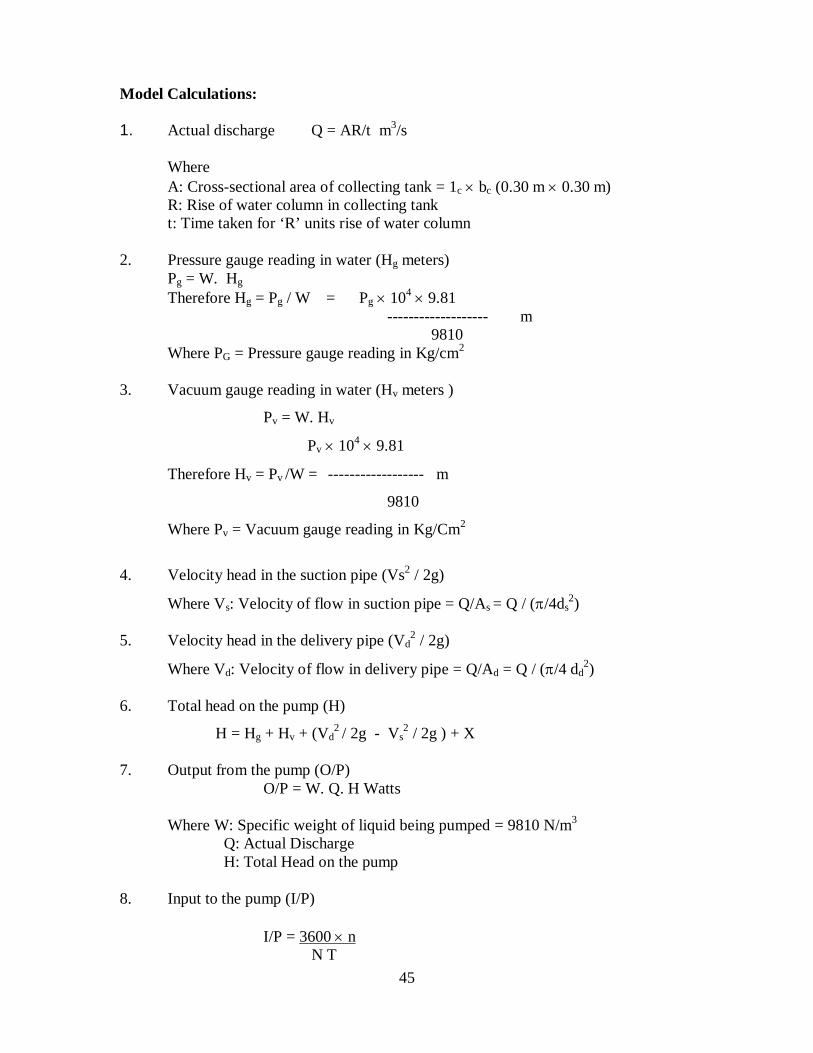
Model Calculations: 1. Actual discharge Q = AR/t m3/s

Where A: Cross-sectional area of collecting tank = 1c bc (0.30 m 0.30 m) R: Rise of water column in collecting tank t: Time taken for ‘R’ units rise of water column

2. Pressure gauge reading in water (Hg meters) Pg = W. Hg

Therefore Hg = Pg / W = Pg 104 9.81 ------------------- m 9810 Where PG = Pressure gauge reading in Kg/cm2 3. Vacuum gauge reading in water (Hv meters )

Pv = W. Hv

Pv 104 9.81

Therefore Hv = Pv /W = ------------------ m

9810

Where Pv = Vacuum gauge reading in Kg/Cm2

4. Velocity head in the suction pipe (Vs2 / 2g)

Where Vs: Velocity of flow in suction pipe = Q/As = Q / (/4ds2)

5. Velocity head in the delivery pipe (Vd

2 / 2g)

Where Vd: Velocity of flow in delivery pipe = Q/Ad = Q / (/4 dd2)

6. Total head on the pump (H)

H = Hg + Hv + (Vd2 / 2g - Vs

2 / 2g ) + X 7. Output from the pump (O/P) O/P = W. Q. H Watts

Where W: Specific weight of liquid being pumped = 9810 N/m3

Q: Actual Discharge H: Total Head on the pump 8. Input to the pump (I/P) I/P = 3600 n N T

46

Where n: Number of revolutions of the energy meter

N: Energy meter constant (rev/kWh)

T: Time taken for ‘n’ revolutions of energy meter

9. Overall efficiency of the pump ( ) (O/P) Efficiency = ------ 100 (I/P) Observation Table Sl No

Press.Gauge Readings

Vacuum Gauge

Readings

Height of

Pressure gauge above

vacuum gauges (x .m.)

Total Head ‘h’

in m

Time for 0.2 m rise in

collecting tank

T seconds

Time for 10 rev. in energy meter T seconds

Actual Disch-arge Qa in m3/S

Out put kw

Input kw

Effi-ciency

1

2

3

4

Graph: See page No.1122 of FM & HM by Modi & Seth for

operating characteristics curves Also for fig see page No.1094 of the above text book


1. What is positive displacement pump? Give examples. 2. What is the effect of accelerator lead on power requirement 3. Why the speed of the pump is kept minimum? 4. What is the effect of friction head at the beginning/ the end of the

stroke(suction/directly) 5. What are uses of air vessel?

47

GEAR OIL PUMP Date: Experiment No.14 Learning Objectives: At the end of this experiment, the student will be able to:

Know the performance characteristics of a gear oil pump. Know the applications of gear oil pump.

Aim: To study the performance characteristics of a gear oil pump. Model:

Fig. Gear Oil Pump

Tools required: Two pressure gauges, stop watch, tachometer and energy meter Procedure:

1. Fill the reservoir tank to about 3/4th capacity with any standard lube oil (SAE

40).

2. Keep the delivery valve open partly and start the pump set.

3. Run the pump at a particular head. This can be adjusted with the help of the

delivery valve.

48

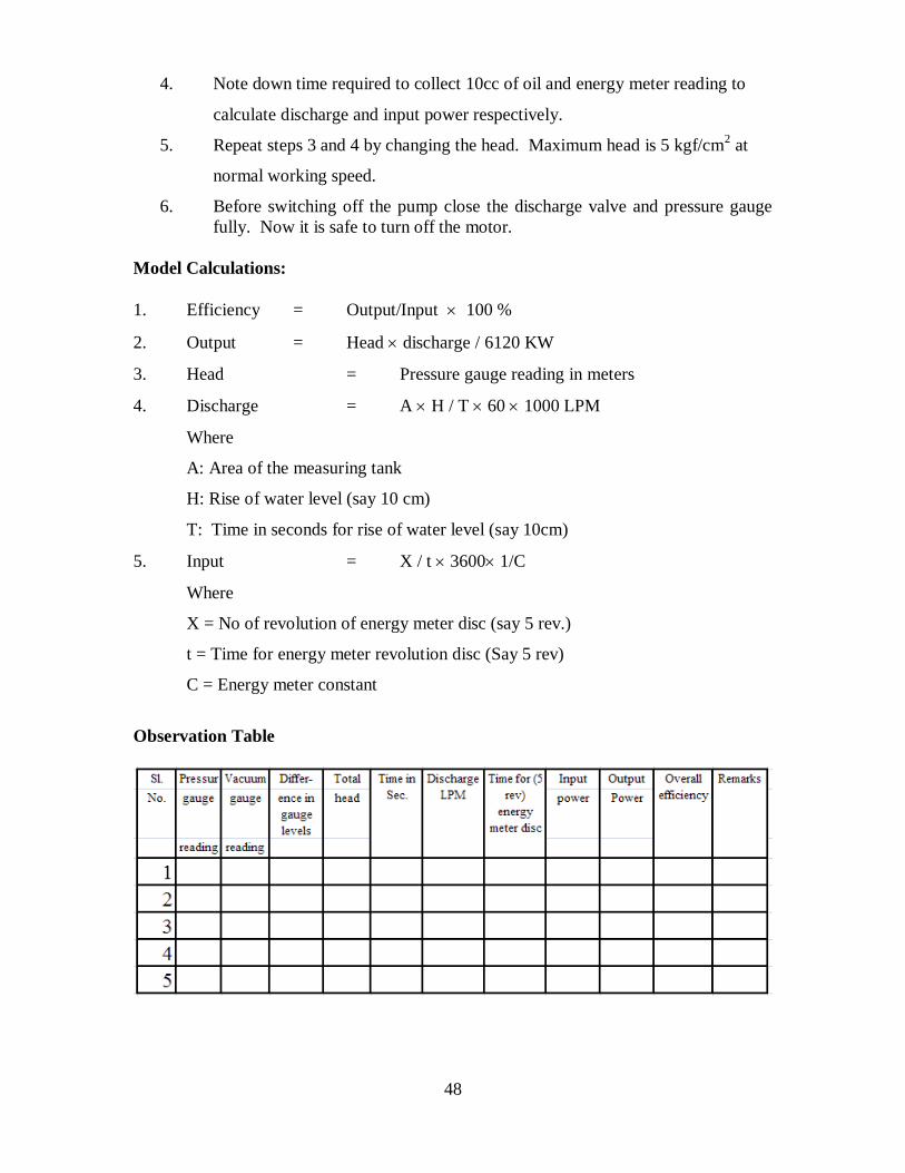
4. Note down time required to collect 10cc of oil and energy meter reading to

calculate discharge and input power respectively.

5. Repeat steps 3 and 4 by changing the head. Maximum head is 5 kgf/cm2 at

normal working speed.

6. Before switching off the pump close the discharge valve and pressure gauge fully. Now it is safe to turn off the motor.

Model Calculations: 1. Efficiency = Output/Input 100 %

2. Output = Head discharge / 6120 KW

3. Head = Pressure gauge reading in meters

4. Discharge = A H / T 60 1000 LPM

Where

A: Area of the measuring tank

H: Rise of water level (say 10 cm)

T: Time in seconds for rise of water level (say 10cm)

5. Input = X / t 3600 1/C

Where

X = No of revolution of energy meter disc (say 5 rev.)

t = Time for energy meter revolution disc (Say 5 rev)

C = Energy meter constant

Observation Table

49

Graph: The following graphs can be drawn.

(a) Discharge Vs Total head

(b) Discharge Vs Power input

(c) Discharge Vs Efficiency

Result: Review Questions: 1. What will happen if I put Gear Oil instead of engine oil in a generator engine? 2. What are the applications of gear oil pump? 3. What are the types of gear pumps?

50

PELTON WHEEL


Know the working of a Pelton wheel. Draw the characteristic curves of Pelton turbine under constant head and constant

speed. Aim: To determine the characteristic curves of Peloton wheel under constant

head and constant speed. Model: Stop watch and measured weights etc.

51

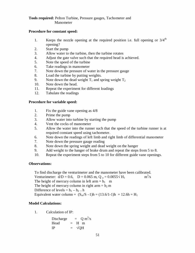
Tools required: Pelton Turbine, Pressure gauges, Tachometer and Manometer

Procedure for constant speed:

1. Keeps the nozzle opening at the required position i.e. full opening or 3/4th opening?

2. Start the pump 3. Allow water to the turbine, then the turbine rotates 4. Adjust the gate valve such that the required head is achieved. 5. Note the speed of the turbine 6. Take readings in manometer 7. Note down the pressure of water in the pressure gauge 8. Load the turbine by putting weights. 9. Note down the dead weight T1 and spring weight T2 10. Note down the head. 11. Repeat the experiment for different loadings 12. Tabulate the readings

Procedure for variable speed:

1. Fix the guide vane opening as 4/8 2. Prime the pump 3. Allow water into turbine by starting the pump 4. Vent the cocks of manometer 5. Allow the water into the runner such that the speed of the turbine runner is at

required constant speed using tachometer. 6. Note down the readings of left limb and right limb of differential manometer 7. Note down the pressure gauge reading 8. Note down the spring weight and dead weight on the hanger 9. Add weight to the hanger of brake drum and repeat the steps from 5 to 8. 10. Repeat the experiment steps from 5 to 10 for different guide vane openings.

Observations:

To find discharge the venturimeter and the manometer have been calibrated. Venturimeter: d/D = 0.6, D = 0.065 m, Q a = 0.0055√ H1 m3/s The height of mercury column in left arm = h1 m The height of mercury column in right arm = h2 m Difference of levels = h1 – h2 = h Equivalent water column = (Sm/S –1)h = (13.6/1-1)h = 12.6h = H1

Model Calculations:

1. Calculation of IP:

Discharge = Q m3/s Head = H m IP = QH

52

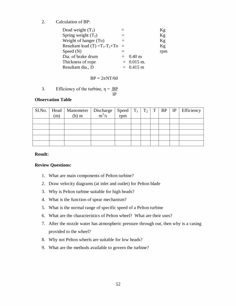
2. Calculation of BP:

Dead weight (T1) = Kg Spring weight (T2) = Kg Weight of hanger (To) = Kg Resultant load (T) =T1-T2+To = Kg Speed (N) = rpm Dia. of brake drum = 0.40 m Thickness of rope = 0.015 m. Resultant dia., D = 0.415 m

BP = 2NT/60

3. Efficiency of the turbine, η = BP IP

Observation Table Sl.No. Head

(m) Manometer

(h) m Discharge

m3/s Speed rpm

T1 T2 T BP IP Efficiency


1. What are main components of Pelton turbine?

2. Draw velocity diagrams (at inlet and outlet) for Pelton blade

3. Why is Pelton turbine suitable for high heads?

4. What is the function of spear mechanism?

5. What is the normal range of specific speed of a Pelton turbine

6. What are the characteristics of Pelton wheel? What are their uses?

7. After the nozzle water has atmospheric pressure through out, then why is a casing

provided to the wheel?

8. Why not Pelton wheels are suitable for low heads?

9. What are the methods available to govern the turbine?

53

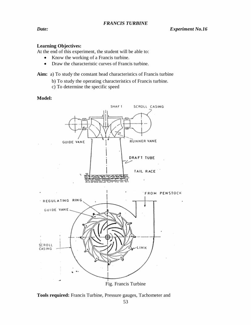
FRANCIS TURBINE Date: Experiment No.16 Learning Objectives: At the end of this experiment, the student will be able to:

Know the working of a Francis turbine. Draw the characteristic curves of Francis turbine.

Aim: a) To study the constant head characteristics of Francis turbine b) To study the operating characteristics of Francis turbine.

c) To determine the specific speed Model:

Fig. Francis Turbine

Tools required: Francis Turbine, Pressure gauges, Tachometer and

54

Manometer Procedure for constant head operation of turbine:

1. Fix the guide vane opening as 4/8. 2. Prime the pump 3. Allow water in the turbine by starting the pump 4. Vent the cocks of manometer 5. Adjust the gate valve such that the sum of the pressure gauge and vacuum

gauge is as required constant head. 6. Note down the pressure gauge and vacuum gauge readings. 7. Note down the left limb and right limb of the differential manometer. 8. Note down the spring weight and dead weight on hanger. 9. Measure the speed of the turbine using tachometer. 10. Repeat the experiment by adding loads on the brake drum 11. Repeat the steps from 1 to 10 for different guide vane opening.

Procedure for variable speed head operation of turbine:

1. Fix the guide vane opening as 4/8. 2. Prime the pump 3. Allow water into turbine by starting the pump 4. Vent the cocks of manometer. 5. Allow the water into the runner such that the speed of the turbine runner is at

required constant speed using tachometer. 6. Note down the left limb and right limb of differential manometer. 7. Note down the pressure gauge and vacuum gauge readings. 8. Note down the spring weight and dead weight on the hanger. 9. Add weight to the hanger of brake drum repeat the steps from 5 to 8. 10. Repeat the experiment steps from 5 to 9 for different guide vane openings.

Model Calculations:

a) Discharge formula for venturimeter Q=0.031√H1

Where H1=12.6h.

h = difference in the levels of manometer.

b) Total head H = G+V

Where G= pressure head V=Vaccum head

c) Input to the turbine IP = Q H

d) Output

55

Brake drum diameter = 0.3 m Pipe diameter = 0.015 m. Equivalent drum diameter = 0.315 m Hanger weight To= 1 kg. Load weight = T1 kg. Spring weight = T2 Kg. Resultant load T= (T1+T0-T2) kg. Speed of turbine = N rpm. BP = 2 NT/60

e) Efficiency (o) = Output = BHP

Input IHP

f) Specific speed: It may be defined as the speed of geometrically similar turbine

which will develop one unit power under unit head.

Ns = N √P H5/4


1. What is the function of draft tube?

2. What is the function of guide vanes?

3. Can you locate the portion in Francis turbine where cavitations likely to occur?

4. What is the advantage of draft tube divergent over a cylindrical of uniform

diameter along its length?

5. What are fast, medium by slow runners?

56

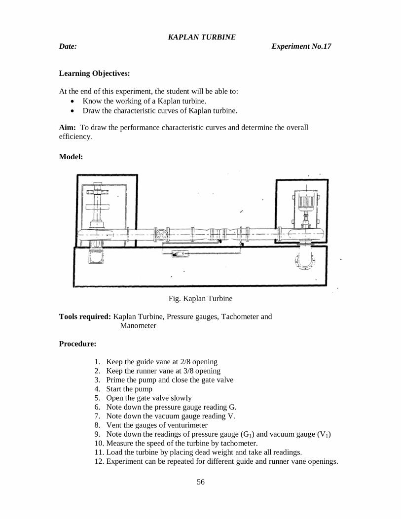
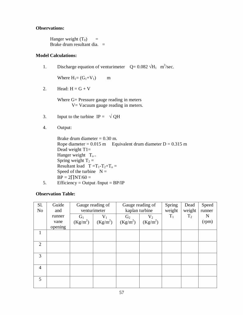
KAPLAN TURBINE Date: Experiment No.17 Learning Objectives: At the end of this experiment, the student will be able to:

Know the working of a Kaplan turbine. Draw the characteristic curves of Kaplan turbine.

Aim: To draw the performance characteristic curves and determine the overall efficiency. Model:

Fig. Kaplan Turbine

Tools required: Kaplan Turbine, Pressure gauges, Tachometer and

Manometer Procedure:

1. Keep the guide vane at 2/8 opening 2. Keep the runner vane at 3/8 opening 3. Prime the pump and close the gate valve 4. Start the pump 5. Open the gate valve slowly 6. Note down the pressure gauge reading G. 7. Note down the vacuum gauge reading V. 8. Vent the gauges of venturimeter 9. Note down the readings of pressure gauge (G1) and vacuum gauge (V1) 10. Measure the speed of the turbine by tachometer. 11. Load the turbine by placing dead weight and take all readings. 12. Experiment can be repeated for different guide and runner vane openings.

57

Observations:

Hanger weight (T0) = Brake drum resultant dia. =

Model Calculations:

1. Discharge equation of venturimeter Q= 0.082H1 m3/sec. Where H1= (G1+V1) m

2. Head: H = G + V

Where G= Pressure gauge reading in meters V= Vacuum gauge reading in meters.

3. Input to the turbine IP = QH

4. Output:

Brake drum diameter = 0.30 m. Rope diameter = 0.015 m Equivalent drum diameter D = 0.315 m Dead weight T1= Hanger weight To = Spring weight T2 = Resultant load T =T1-T2+To = Speed of the turbine N = BP = 2NT/60 =

5. Efficiency = Output /Input = BP/IP Observation Table: Sl. No

Guide and

runner vane

opening

Gauge reading of venturimeter

Gauge reading of kaplan turbine

Spring weight

T1

Dead weight

T2

Speed runner

N (rpm)

G1 (Kg/m2)

V1 (Kg/m2)

G2 (Kg/m2)

V2 (Kg/m2)

1

2

3

4

5

58

Graphs:

1) % of full load Vs o 2) N u Vs Q u or Pu or o Result: Review Questions:

1. What are suitable conditions for erection of Kaplan turbine

2. Why is the number of blades of Kaplan turbine restricted to 4 to 6?

3. Is this turbine axial flow or mixed flow?

4. Port load efficiency of Kaplan turbine is high, why?

5. What is the minimum pressure that can be maintained at the exit of the reaction

turbine?

59

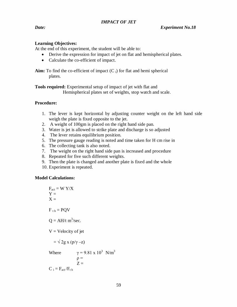
IMPACT OF JET Date: Experiment No.18


Derive the expression for impact of jet on flat and hemispherical plates. Calculate the co-efficient of impact.

Aim: To find the co-efficient of impact (C i) for flat and hemi spherical

plates. Tools required: Experimental setup of impact of jet with flat and

Hemispherical plates set of weights, stop watch and scale. Procedure:

1. The lever is kept horizontal by adjusting counter weight on the left hand side weigh the plate is fixed opposite to the jet.

2. A weight of 100gm is placed on the right hand side pan. 3. Water is jet is allowed to strike plate and discharge is so adjusted 4. The lever retains equilibrium position. 5. The pressure gauge reading is noted and time taken for H cm rise in 6. The collecting tank is also noted. 7. The weight on the right hand side pan is increased and procedure 8. Repeated for five such different weights. 9. Then the plate is changed and another plate is fixed and the whole 10. Experiment is repeated.

Model Calculations:

Fact = W Y/X Y = X = F t h = PQV Q = AH/t m3/sec. V = Velocity of jet = √ 2g x (p/γ –z) Where γ = 9.81 x 103 N/m3

ρ = Z =

C i = Fact /Ft h

60

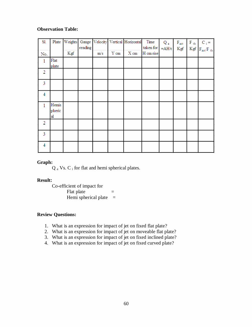
Observation Table:

Graph:

Q a Vs. C i for flat and hemi spherical plates. Result:

Co-efficient of impact for Flat plate = Hemi spherical plate =

Review Questions:

1. What is an expression for impact of jet on fixed flat plate? 2. What is an expression for impact of jet on moveable flat plate? 3. What is an expression for impact of jet on fixed inclined plate? 4. What is an expression for impact of jet on fixed curved plate?

61

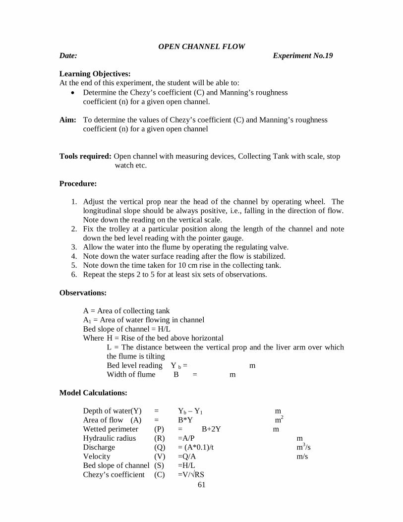
OPEN CHANNEL FLOW


Determine the Chezy’s coefficient (C) and Manning’s roughness coefficient (n) for a given open channel.

Aim: To determine the values of Chezy’s coefficient (C) and Manning’s roughness

coefficient (n) for a given open channel Tools required: Open channel with measuring devices, Collecting Tank with scale, stop

watch etc. Procedure:

1. Adjust the vertical prop near the head of the channel by operating wheel. The longitudinal slope should be always positive, i.e., falling in the direction of flow. Note down the reading on the vertical scale.

2. Fix the trolley at a particular position along the length of the channel and note down the bed level reading with the pointer gauge.

3. Allow the water into the flume by operating the regulating valve. 4. Note down the water surface reading after the flow is stabilized. 5. Note down the time taken for 10 cm rise in the collecting tank. 6. Repeat the steps 2 to 5 for at least six sets of observations.

Observations:

A = Area of collecting tank A1 = Area of water flowing in channel Bed slope of channel = H/L Where H = Rise of the bed above horizontal

L = The distance between the vertical prop and the liver arm over which the flume is tilting Bed level reading Y b = m

Width of flume B = m Model Calculations:

Depth of water(Y) = Yb – Y1 m Area of flow (A) = B*Y m2 Wetted perimeter (P) = B+2Y m Hydraulic radius (R) =A/P m Discharge (Q) = (A*0.1)/t m3/s Velocity (V) =Q/A m/s Bed slope of channel (S) =H/L Chezy’s coefficient (C) =V/√RS

62

Manning’s coefficient (n) = (R2/3 S1/2)/V

Observation Table: Sl.No. Water surface reading

Y1 m Depth of water

(Y) = (Yb - Y1) m

Area of flow A o = B * Y

m2

Wetted perimeter

P = (B+2Y)

1 2 3 4 5

Hydraulic radius

R = A o/P M

Time taken for 10 cm rise in

collecting tank t sec.

Discharge Q =( A*0.1)/t

m3/s

Velocity V=Q/A1

m/s C = V/√RS

R2/3 S1/2

V = n

6 7 8 9 10 11 Graphs:

1. V Vs. √RS 2. V Vs. (R2/3 S1/2) Result: Chezy’s coefficient C = Manning’s coefficient n = Review Questions:

1. What do you mean by an open channel flow? 2. Can flow through (a pipe) closed conduit be open channel flow? 3. What governs open channel flow? 4. Is the velocity distribution uniform. If not, why? 5. Where do you expect to have maximum velocity in an open channel? 6. What factors affect the velocity distribution in an open channel? 7. What is ? 8. What is ? 9. What are the possible values of and?

63

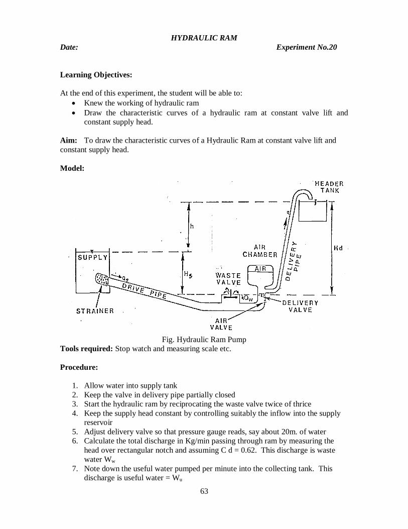
HYDRAULIC RAM Date: Experiment No.20


Knew the working of hydraulic ram Draw the characteristic curves of a hydraulic ram at constant valve lift and

constant supply head. Aim: To draw the characteristic curves of a Hydraulic Ram at constant valve lift and constant supply head. Model:

Fig. Hydraulic Ram Pump


1. Allow water into supply tank 2. Keep the valve in delivery pipe partially closed 3. Start the hydraulic ram by reciprocating the waste valve twice of thrice 4. Keep the supply head constant by controlling suitably the inflow into the supply

reservoir 5. Adjust delivery valve so that pressure gauge reads, say about 20m. of water 6. Calculate the total discharge in Kg/min passing through ram by measuring the

head over rectangular notch and assuming C d = 0.62. This discharge is waste water Ww

7. Note down the useful water pumped per minute into the collecting tank. This discharge is useful water = Wu

64

8. Note down the time taken for 50 beasts and calculate per minute 9. Repeat the experiment for six different delivery heads at intervals of 3 to 4m

water. Let Hs be the supply head in m. of water and H d the delivery head in m. of water. Hs are the height of water surface in the reservoir above waste valve.Hd is the pressure gauge reading and difference in level between the center of the gauge and waste valve.

Model Calculations: Wu (H d – Hs)

(a) Rankin Efficiency = ----------------- choosing supply water surface as datum W w Hs

W u H d (b) D ‘Abuissons’ Efficiency = ---------------

(W w + W u) Hs

choosing the datum plane as that passing through waste valve. Graphs:

The following graphs are drawn. H d Vs D ‘Abuissons’ Efficiency H d Vs Waste Water/min = Ww H d Vs Beats/min. H d Vs Useful water/min = Wu H d Vs Rankine Efficiency


1. What is the principle of hydraulic ram?

2. Applications of hydraulic ram.

3. What is the difference between hydraulic ram and pneumatic ram?

4. Define hydraulic accumulator

fluid mechanics and machinery laboratoryfiles.kluceb.webnode.in/200000041-72634735b1/fm...

Documents