fluid mechanics and climate dynamics · fluid mechanics and climate dynamics: observations,...
TRANSCRIPT
Fluid Mechanics and Climate Dynamics:
Observations, Simulations and (Maybe) Predictions
Michael GhilEcole Normale Supérieure, Paris, and
University of California, Los Angeles
Please see these sites for collaborators and further details:http://www.environnement.ens.fr/
http://e2c2.ipsl.jussieu.fr/
http://www.atmos.ucla.edu/tcd/
Special thanks to Mickaël Chekroun and Eric Simonnet!
EE250 Conference Aussois, 19–22 June 2007

Motivation
• The climate system is highly nonlinear and quite complex.
• Its major components — the atmosphere, oceans, ice sheets— flow on many time and space scales.
• Its predictive understanding has to rely on the system!sphysical, chemical and biological modeling,
but also on the mathematical analysis of the models
thus obtained.
• The hierarchical modeling approach allows one to
give proper weight to the understanding provided by the
models vs. their realism, respectively.
• This approach facilitates the evaluation of forecasts(pognostications?) based on these models.
• Back-and-forth between “toy” (conceptual) and detailed(“realistic”) models, and between models and data.

Global warming and
its socio-economic impacts
Temperatures rise:
• What about impacts?
• How to adapt?
Source : IPCC (2001),
TAR, WGI, SPM

GHGs rise
It’s gotta do with us, at
least a bit, ain’t it?
IPCC (2001)

But things aren’t that easy!What to do?
• Natural variability introducesadditional complexity into theanthropogenic climate change problem.
• The most common interpretation of observations andGCM simulations of climate change is still in terms ofa scalar, linear ordinary differential equation (ODE):
cdT
dt= !kT + Q,
where
k =!
ki ! feedbacks (+ve and –ve);
Q =!
Qj ! sources & sinks, Qj = Qj(t)
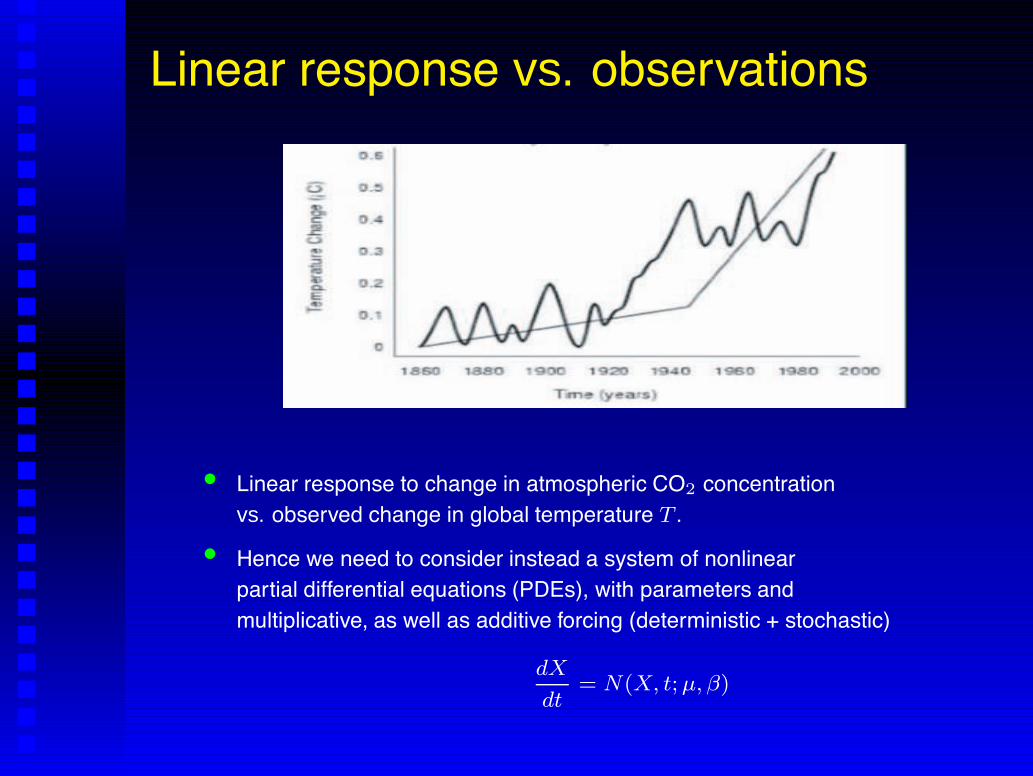
Linear response vs. observations
• Linear response to change in atmospheric CO2 concentrationvs. observed change in global temperature T .
• Hence we need to consider instead a system of nonlinearpartial differential equations (PDEs), with parameters andmultiplicative, as well as additive forcing (deterministic + stochastic)
dX
dt= N(X, t; µ, !)

Composite spectrum of climate variability
Standard treatement of frequency bands:
1. High frequencies – white (or !!colored"") noise
2. Low frequencies – slow (!!adiabatic"") evolution of parameters
From Ghil (2001, EGEC), after Mitchell* (1976)
* !!No known source of deterministic internal variability""
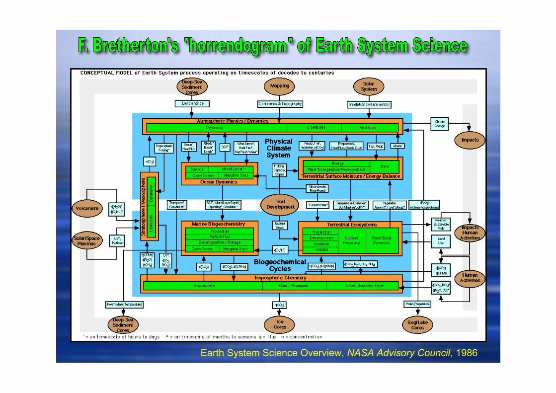
Earth System Science Overview, NASA Advisory Council, 1986
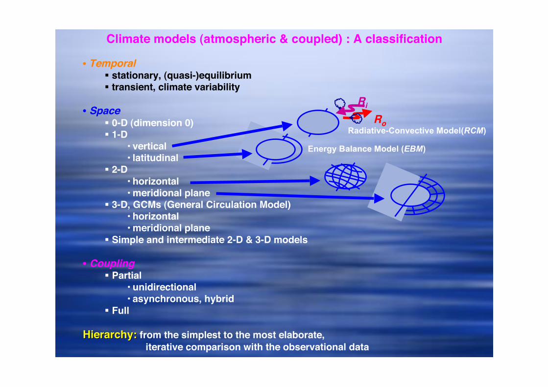
• Temporal! stationary, (quasi-)equilibrium! transient, climate variability
• Space! 0-D (dimension 0)! 1-D
• vertical• latitudinal
! 2-D• horizontal• meridional plane
! 3-D, GCMs (General Circulation Model)• horizontal• meridional plane
! Simple and intermediate 2-D & 3-D models
• Coupling! Partial
• unidirectional• asynchronous, hybrid
! Full
HierarchyHierarchy:: from the simplest to the most elaborate,
iterative comparison with the observational data
Climate models (atmospheric & coupled) : A classification
Radiative-Convective Model(RCM)
Energy Balance Model (EBM)
Ro
Ri
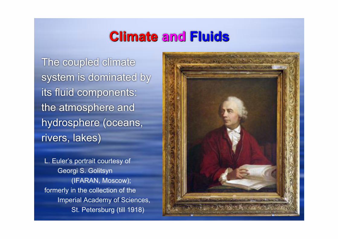
ClimateClimate andand FluidsFluids
The coupled climate
system is dominated by
its fluid components:
the atmosphere and
hydrosphere (oceans,
rivers, lakes)
L. Euler’s portrait courtesy of
Georgi S. Golitsyn
(IFARAN, Moscow);
formerly in the collection of the
Imperial Academy of Sciences,
St. Petersburg (till 1918)
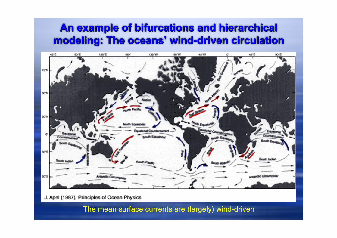
An example of bifurcations and hierarchicalAn example of bifurcations and hierarchical
modeling: The oceansmodeling: The oceans’’ wind-driven circulation wind-driven circulation
The mean surface currents are (largely) wind-driven

The gyres and the eddiesThe gyres and the eddies
Many scales of motion,
dominated in the
mid-latitudes by
(i) the double-gyre circulation;
and (ii) the rings and eddies.
Based on SSTs, from satellite IR data
Much of the focus of physical
oceanography over the "70s to
"90s has been with the
“meso-scale”: the meanders,
rings & eddies, and the
associated two-dimensional and
quasi-geostrophic turbulence.

The double-gyre circulationand its low-frequency variabilityShallow-water model: An "intermediate" modelof the mid-latitude, wind-driven ocean circulation,with 20-km resolution! about 15 000 variables.
!
"
"
"
#
"
"
"
$
Ut + " · (uU) = #g!hhx + fV + !AA"2U # RU # !!!x
"
Vt + " · (uV ) = #g!hhy # fU + !AA"2V # RV
ht = #(Ux + Vy)
where Uex + V ey = hu = h(uex + vey),g!: reduced gravity, g! = g("2 # ")/"
A: viscosity coefficient (= 300 m2s"1)R: Rayleigh coefficient (= 1/200 day"1)
#x: wind stress = #0 cos(2$/L) (#0 = 1 dyn cm"2& L = 2000 km)
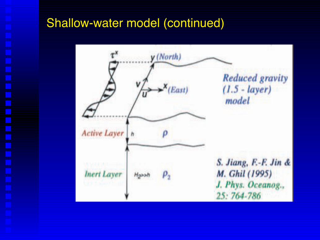
Shallow-water model (continued)

The JJG modelThe JJG model’’s s equilibriaequilibria
Nonlinear (advection)
effects break the (near)
symmetry:
(perturbed) pitchfork
bifurcation?
Subpolar gyre
dominates
Subtropical gyredominates

Time-dependent solutions:Time-dependent solutions:
periodic and chaoticperiodic and chaotic
To capture space-
time dependence,
meteorologists and
oceanographers
often use
Hovmöller diagrams

Poor manPoor man’’s continuation methods continuation method
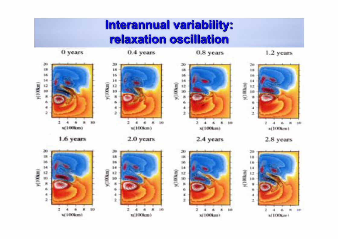
Interannual Interannual variability:variability:
relaxation oscillationrelaxation oscillation

The double-gyre circulation:A different rung of the hierarchyAnother "intermediate" model of the double-gyre circulation:slightly different physics, higher resolution – down to 10-km in thehorizontal and more layers in the vertical, much larger domain, ...Quasi-geostrophic, 2.5-layer model:
!!t(!
2h1 " !21(h1 " h2)) + " !h1
!x = "g!
f0J [h1,!2h1 " F 2
1 (h1 " h2)]
+Ah!4h1 " C!2(h1 " h2) + f0
"0g!H1curl("## )
!!t(!
2h2 " !22(h2 " h1)) + " !h2
!x = "g!
f0J [h2,!2h2 " F 2
2 (h2 " h1)]
+Ah!4h2 " C!2(h2 " h1) " R!2h2
where h1, h2: height anomalies for upper and lower layerH1, H2 : mean heights for upper and lower layer#1, #2 : Rossby radii of deformation; #1 = h!H1/f2
0, #2 = h!H2/f2
0
f0, $ : Coriolis and beta parameters"0, g!: mean density and reduced gravity
C, R: Rayleigh coefficient for interface and lower layer, and!"% : wind stress
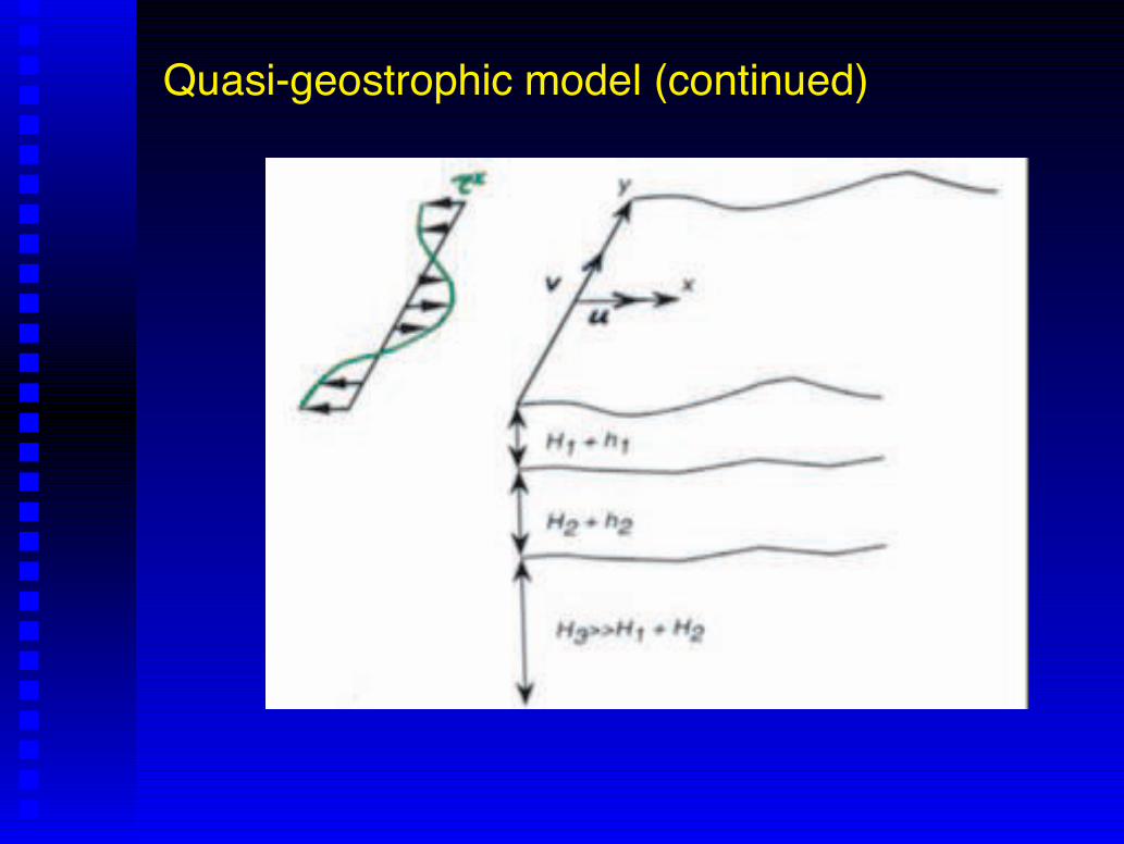
Quasi-geostrophic model (continued)
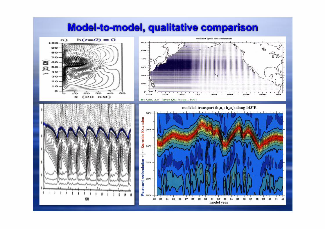
Model-to-model, qualitative comparisonModel-to-model, qualitative comparison
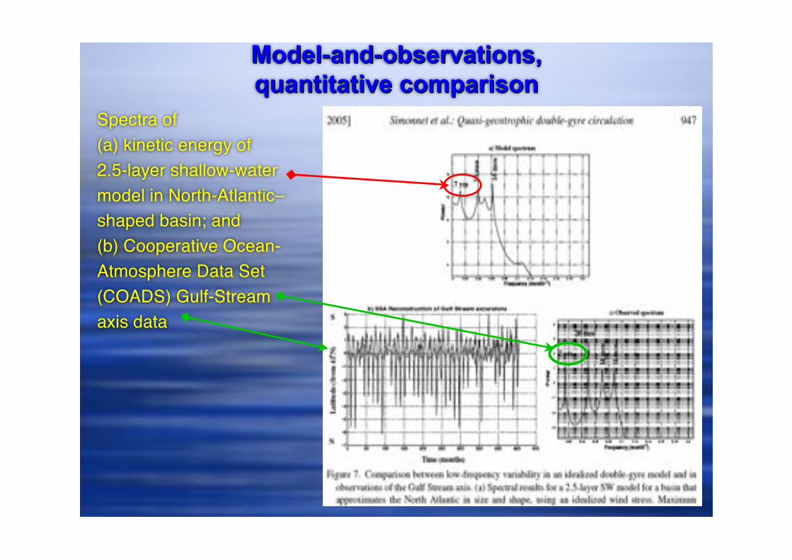
Model-and-observations,Model-and-observations,
quantitative comparisonquantitative comparison
Spectra of
(a) kinetic energy of
2.5-layer shallow-water
model in North-Atlantic–
shaped basin; and
(b) Cooperative Ocean-
Atmosphere Data Set
(COADS) Gulf-Stream
axis data

More More spatio-temporal spatio-temporal datadata
Multi-channel SSA
analysis of the UK
Met Office monthly
mean SSTs for the
century-long
1895–1994 interval
Marked similarity with the
7–8-year “gyre mode” of
a full hierarchy of ocean
models, on the one hand,
and with the North
Atlantic Oscillation (NAO),
on the other: explanation?
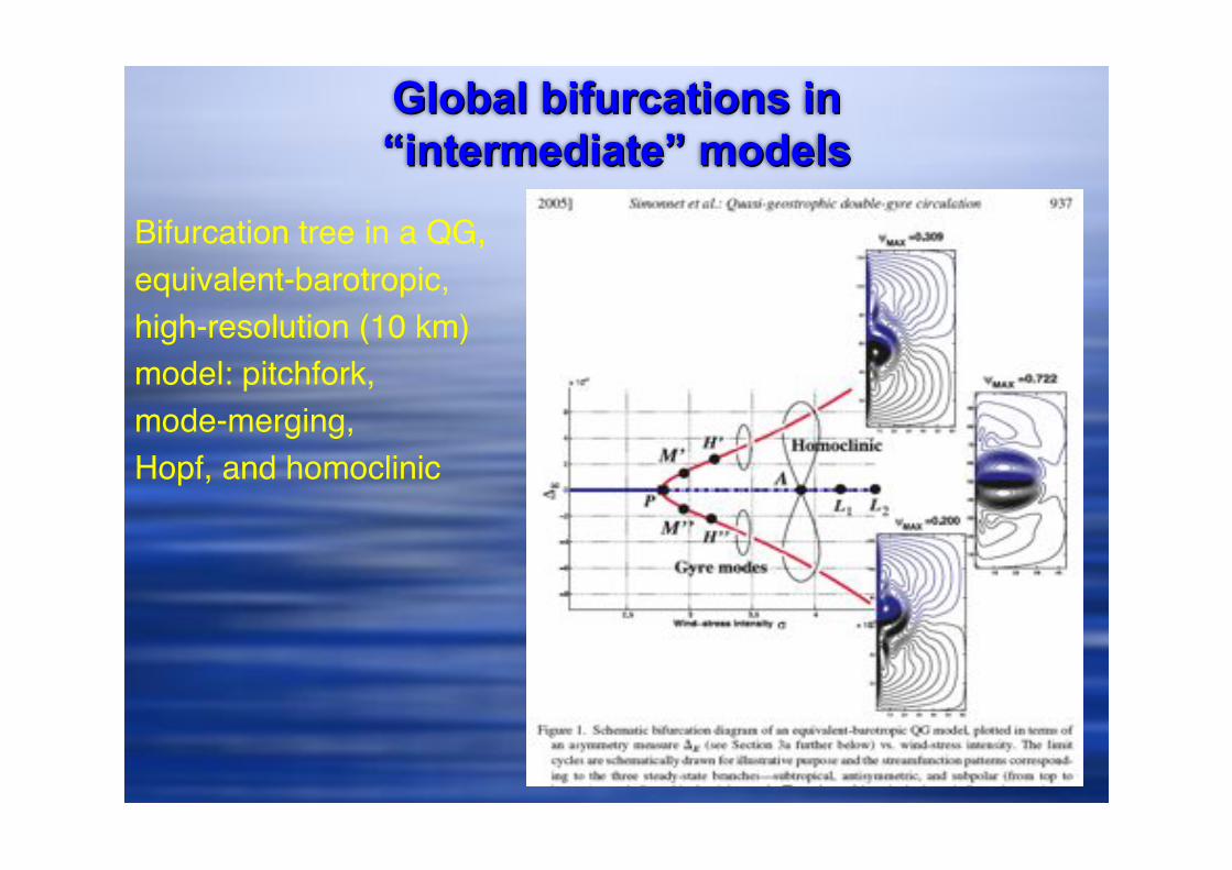
Global bifurcations inGlobal bifurcations in
““intermediateintermediate”” models models
Bifurcation tree in a QG,
equivalent-barotropic,
high-resolution (10 km)
model: pitchfork,
mode-merging,
Hopf, and homoclinic

Homoclinic Homoclinic orbit: numerical and analyticalorbit: numerical and analytical

Uncertainties in the forcingUncertainties in the forcing
Contributions to the
forcing, natural and
anthropogenic, also
have substantial
uncertainties
Source : IPCC (2001),
TAR, WGI, SPM

So whatSo what’’s it s it gonna gonna be like, by 2100?be like, by 2100?
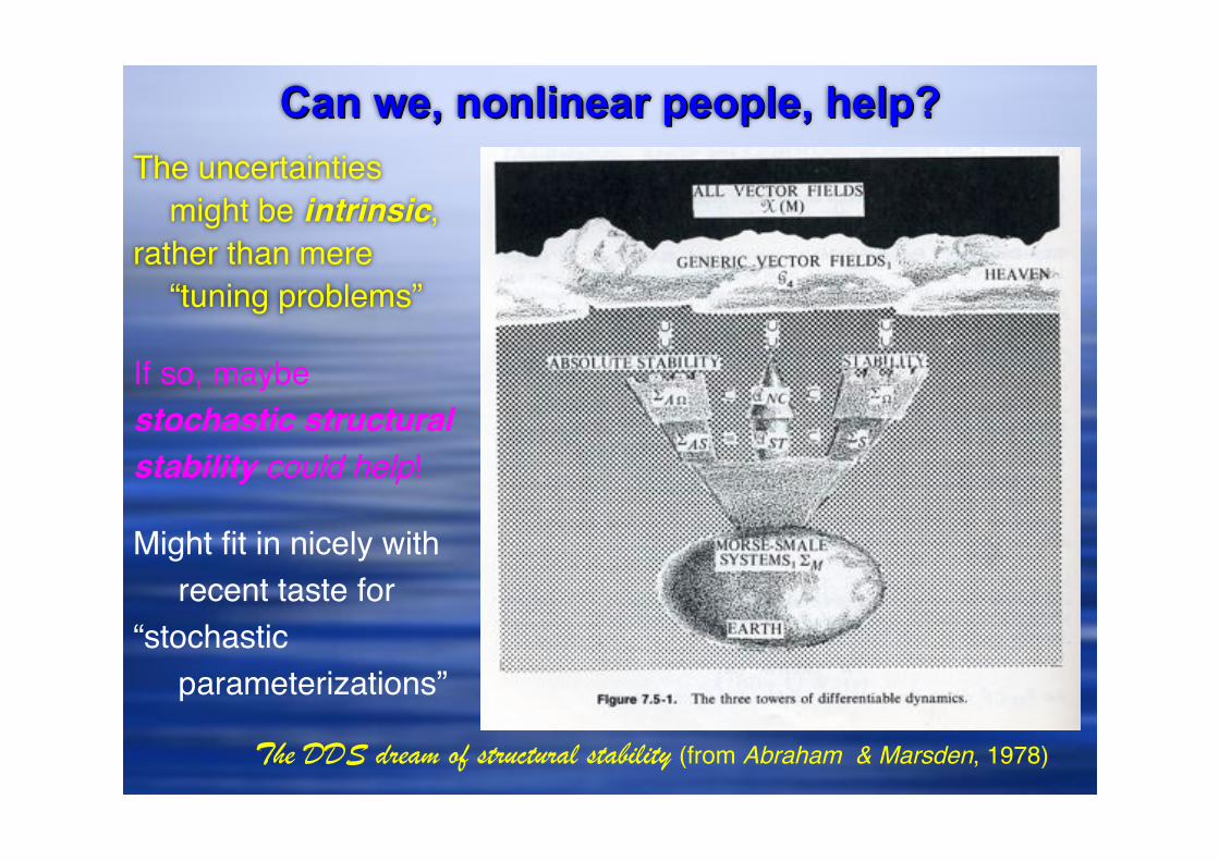
Can we, nonlinear people, help?Can we, nonlinear people, help?
The uncertainties
might be intrinsic,
rather than mere
“tuning problems”
If so, maybe
stochastic structural
stability could help!
The DDS dream of structural stability (from Abraham & Marsden, 1978)
Might fit in nicely with
recent taste for
“stochastic
parameterizations”
Random Dynamical Systems – RDS
• This theory is a combination ofmeasure (probability) theoryand dynamical systems,initiated by the "Bremen group"(L. Arnold, 1998).
Random Dynamical Systems – RDS
• This theory is a combination ofmeasure (probability) theoryand dynamical systems,initiated by the "Bremen group"(L. Arnold, 1998).
• It allows one to treatstochastic differential equations (SDEs),and more general systemsdriven by some “noise", as flows.
The setting of RDS theory• A phase space X. Example: Rn.
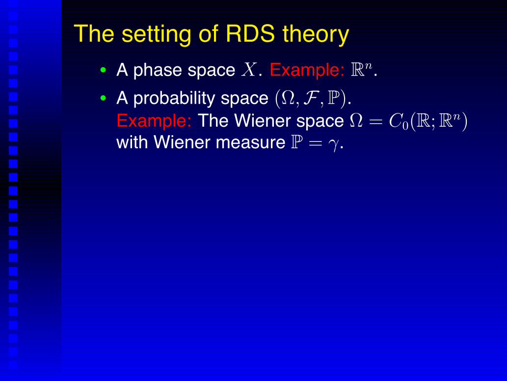
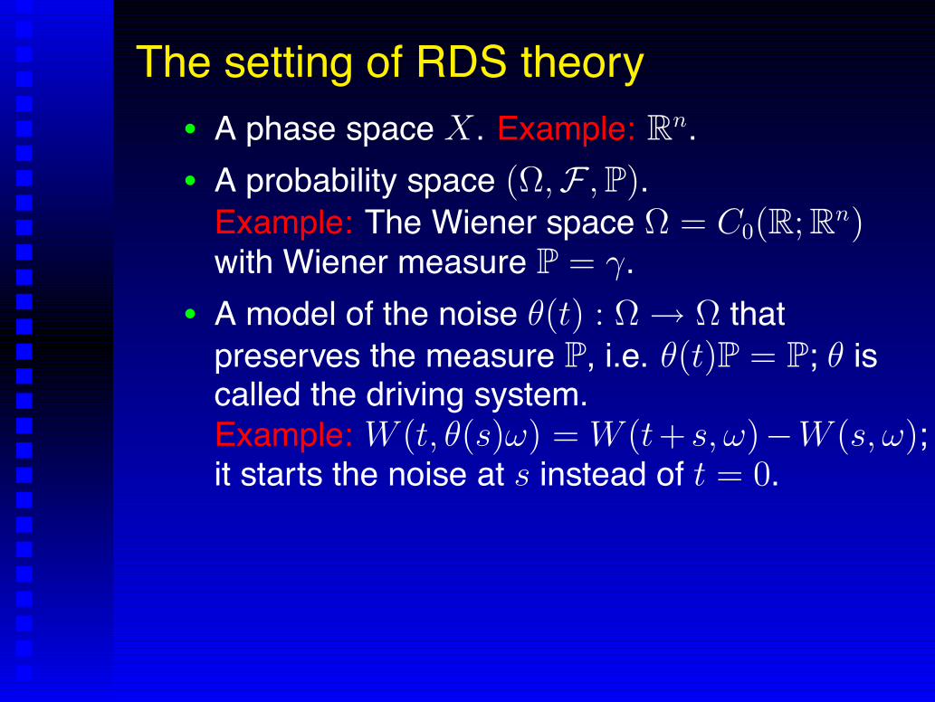
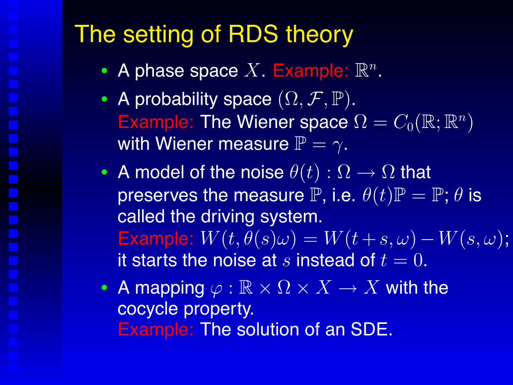
The setting of RDS theory• A phase space X. Example: Rn.• A probability space (!,F , P).Example: The Wiener space ! = C0(R; Rn)with Wiener measure P = !.
The setting of RDS theory• A phase space X. Example: Rn.• A probability space (!,F , P).Example: The Wiener space ! = C0(R; Rn)with Wiener measure P = !.
• A model of the noise "(t) : ! ! ! thatpreserves the measure P, i.e. "(t)P = P; " iscalled the driving system.Example: W (t, "(s)#) = W (t+ s,#)"W (s,#);it starts the noise at s instead of t = 0.
• A mapping $ : R # ! # X ! X with thecocycle property.Example: The solution of an SDE.

RDS – A geometric view of SDEs
!( ,")s
#( )"s#( )"s+t
!( ,")t+s
!( ,")sx
" $
xCocycle property:
!( ,#( )")t s
{#( )"}xs
{"}x X
X{#( )"}s+t xX
x!( ,")t+s
!( ,#( )")t ]=[ x!( ,")ss
• ! is a random dynamical system (RDS)• !(t)(x,") = (#(t)",!(t,")x)is a flow on the bundle
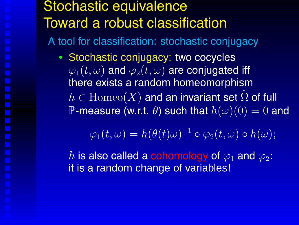
Stochastic equivalenceToward a robust classificationA tool for classification: stochastic conjugacy
• Stochastic conjugacy: two cocycles!1(t,") and !2(t,") are conjugated iffthere exists a random homeomorphismh ! Homeo(X) and an invariant set " of fullP-measure (w.r.t. #) such that h(")(0) = 0 and
!1(t,") = h(#(t)")!1 " !2(t,") " h(");
h is also called a cohomology of !1 and !2:it is a random change of variables!
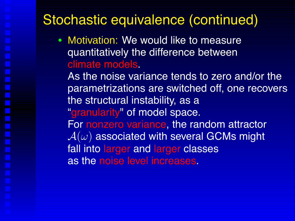
Stochastic equivalence (continued)• Motivation: We would like to measurequantitatively the difference betweenclimate models.As the noise variance tends to zero and/or theparametrizations are switched off, one recoversthe structural instability, as a“granularity" of model space.For nonzero variance, the random attractorA(") associated with several GCMs mightfall into larger and larger classesas the noise level increases.
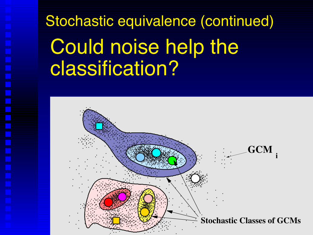
Stochastic equivalence (continued)
Could noise help theclassification?
GCMi
. ...
. ....... . ...
. .... .... ... . ...
. .... .... ....... . ...
. .... .... ... . ...
. .... .... ....... . ...
. .... .... ... . ...
. .... .... ....... . ...
. .... .... ... . ...
. .... .... ....... . ...
. .... .... ... . ...
. .... .... ....... . ...
. .... .... ... . ...
. .... .... ....... . ...
. .... .... ... . ...
. .... .... ....... . ...
. .... .... ... . ...
. .... ...
. ....... . ...
. .... .... ... . ...
. .... .... ....... . ...
. .... .... ... . ...
. .... .... ....... . ...
. .... .... ... . ...
. .... .... ....... . ...
. .... .... ... . ...
. .... .... ....... . ...
. .... .... ... . ...
. .... .... ....... . ...
. .... .... ... . ...
. .... .... ....... . ...
. .... .... ... . ...
. .... .... ....... . ...
. .... .... ... . ...
. .... .... ....... . ...
. .... .... ... . ...
. .... .... ....... . ...
. .... .... ... . ...
. .... ...
. ....... . ...
. .... .... ... . ...
. .... ...
. ....... . ...
. .... .... ... . ...
. .... .... ....... . ...
. .... .... ... . ...
. .... .... ....... . ...
. .... .... ... . ...
. .... .... ....... . ...
. .... .... ... . ...
. .... .... ....... . ...
. .... .... ... . ...
. .... .... ....... . ...
. .... .... ... . ...
. .... .... ....... . ...
. .... .... ... . ...
. .... .... ....... . ...
. .... .... ... . ...
. .... .... ....... . ...
. .... .... ... . ...
. .... ...
. ....... . ...
. .... .... ... . ...
. .... ...
....
..
...
..
...
..
...
. ....
..
...
.
....
.
....
.
....
..
...
..
...
..
...
. ....
..
...
.
....
.
....
.
....
..
...
..
...
..
...
. ....
..
...
.
....
.
....
..
...
..
...
..
...
..
...
. ....
..
...
.
....
.
....
.
....
..
...
..
...
..
...
. ....
..
...
.
....
.
....
.
....
..
...
..
...
..
...
. ....
..
...
.
....
.
....
.
....
..
...
..
...
..
...
. ....
..
...
.
....
.
....
.....
..
...
..
...
..
...
. ....
..
...
.
....
.
....
..
...
..
...
..
...
..
...
. ....
..
...
.
....
.
....
..
...
..
...
..
...
..
...
. ....
..
...
.
....
.
....
..
...
..
...
..
...
..
...
. ....
..
...
.
....
.
....
..
...
..
...
..
...
..
...
. ....
..
...
.
....
.
....
..
...
..
...
..
...
..
...
. ....
..
...
.
....
.
....
.
....
..
...
..
...
..
...
. ....
..
...
.
....
.
....
.
....
..
...
..
...
..
...
. ....
..
...
.
....
.
....
..
...
..
...
..
...
..
...
. ....
..
...
.
....
.
....
.
....
..
...
..
...
..
...
. ....
..
...
.
....
.
....
..
...
..
...
..
...
..
...
. ....
..
...
.
....
.
....
..
...
..
...
..
...
..
...
. ....
..
...
.
....
.
....
..
...
..
...
..
...
..
...
. ....
..
...
.
....
.
....
.....
..
...
..
...
..
...
. ....
..
...
.
....
.
....
.
....
..
...
..
...
..
...
. ....
..
...
.
....
.
....
.
....
..
...
..
...
..
...
. ....
..
...
.
....
.
....
.
....
..
...
..
...
..
...
. ....
..
...
.
....
.
....
.
....
..
...
..
...
..
...
. ....
..
...
.
....
.
....
..
...
..
...
..
...
..
...
. ....
..
...
.
....
.
....
.
....
..
...
..
...
..
...
. ....
..
...
.
....
.
....
.
....
..
...
..
...
..
...
. ....
..
...
.
....
.
....
..
...
..
...
..
...
..
...
. ....
..
...
.
....
.
....
..
...
..
...
..
...
..
...
. ....
..
...
.
....
.
....
.
....
..
...
..
...
..
...
. ....
..
...
.
....
.
....
. ....
..
...
..
...
..
...
. ....
..
...
.
....
.
....
..
...
..
...
..
...
..
...
. ....
..
...
.
....
.
....
..
...
..
...
..
...
..
...
. ....
..
...
.
....
.
....
.
....
..
...
..
...
..
...
. ....
..
...
.
....
.
....
.
....
..
...
..
...
..
...
. ....
..
...
.
....
.
....
.
....
..
...
..
...
..
...
. ....
..
...
.
....
.
....
.
....
..
...
..
...
..
...
. ....
..
...
.
....
.
....
.
....
..
...
..
...
..
...
. ....
..
...
.
....
.
....
.
....
..
...
..
...
..
...
. ....
..
...
.
....
.
....
.
....
..
...
..
...
..
...
. ....
..
...
.
....
.
....
.
....
..
...
..
...
..
...
. ....
..
...
.
....
.
....
. ....
..
...
..
...
..
...
. ....
..
...
.
....
.
....
. ....
..
...
..
...
..
...
. ....
..
...
.
....
.
....
. ....
..
...
..
...
..
...
. ....
..
...
.
....
.
....
.
....
..
...
..
...
..
...
. ....
..
...
.
....
.
....
..
...
..
...
..
...
..
...
. ....
..
...
.
....
.
....
.....
..
...
..
...
..
...
. ....
..
...
.
....
.
....
.
.
.
...
.
..
.
.
...
.
...
.
...
.
..
.
.
...
.
..
.
.
...
.
..
.
.
...
.
..
.
.
...
.
..
.
.
...
.
..
.
.
...
.
..
.
.
...
.
..
.
.
...
.
..
.
.
...
.
..
.
.
...
. ..
...
.
.
...
.
..
.
.
...
.
..
.
.
...
.
..
....
..
...
..
...
..
...
. ....
..
...
.
....
.
....
.....
..
...
..
...
..
...
. ....
..
...
.
....
.
....
.....
..
...
..
...
..
...
. ....
..
...
.
....
.
....
.....
..
...
..
...
..
...
. ....
..
...
.
....
.
....
. ....
..
...
..
...
..
...
. ....
..
...
.
....
.
....
.....
..
...
..
...
..
...
. ....
..
...
.
....
.
....
.
....................
........
............................
........
........
....................
........
........
....................
........
........ ....................
........
............................
........
............................
........
........
....
..
...
..
...
..
...
. ....
.
....
.
....
..
...
..
...
..
...
. ....
.
....
.
....
..
...
..
...
..
...
. ....
..
...
.
....
.
....
..
...
..
...
..
...
. ....
..
...
.
....
.
....
.
....................
........
........
Stochastic Classes of GCMs .
.
...
.
..
.
.
...
.
..
.
.
...
.
..
....
.
....
.....
. ....
. ....
..
...
.
....
..
...
.
........
.
....
..
...
.
....
.
....
.
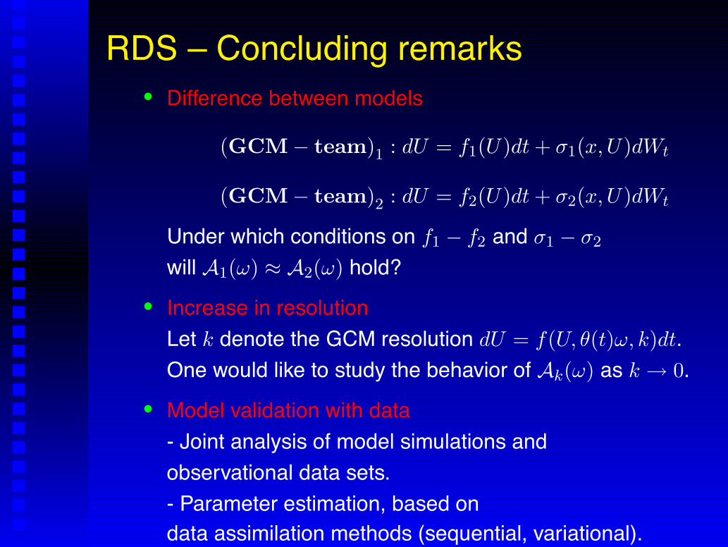
RDS – Concluding remarks• Difference between models
(GCM ! team)1 : dU = f1(U)dt + !1(x,U)dWt
(GCM ! team)2 : dU = f2(U)dt + !2(x,U)dWt
Under which conditions on f1 ! f2 and !1 ! !2
will A1(") " A2(") hold?• Increase in resolutionLet k denote the GCM resolution dU = f(U, #(t)", k)dt.One would like to study the behavior of Ak(") as k # 0.
• Model validation with data- Joint analysis of model simulations andobservational data sets.- Parameter estimation, based ondata assimilation methods (sequential, variational).
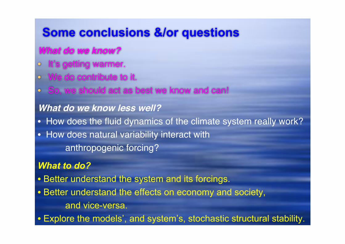
Some conclusions &/or questions
What do we know?
• It!s getting warmer.
• We do contribute to it.
• So, we should act as best we know and can!
What do we know less well?
• How does the fluid dynamics of the climate system really work?
• How does natural variability interact with
anthropogenic forcing?
What to do?
• Better understand the system and its forcings.
• Better understand the effects on economy and society,
and vice-versa.
• Explore the models’, and system’s, stochastic structural stability.

Some general referencesAndronov, A.A., and L.S. Pontryagin, 1937: Systèmes grossiers. Dokl. Akad. Nauk. SSSR,
14(5), 247–250.
Arnold, L., 1998: Random Dynamical Systems, Springer Monographs in Math., Springer, 625 pp.
Charney, J., et al., 1979: Carbon Dioxide and Climate: A Scientific Assesment. NationalAcademic Press, Washington, D.C.
Dijkstra, H.A., 2005: Nonlinear Physical Oceanography: A Dynamical Systems Approach to theLarge-Scale Ocean Circulation and El Niño (2nd edn.), Springer, 532 pp.
Ghil, M., R. Benzi, and G. Parisi (Eds.), 1985: Turbulence and Predictability in Geophysical FluidDynamics and Climate Dynamics, North-Holland,, 449 pp.
Ghil, M., and S. Childress, 1987: Topics in Geophysical Fluid Dynamics:
Atmospheric Dynamics, Dynamo Theory and Climate Dynamics, Springer, 485 pp.
Ghil, M., 2001: Hilbert problems for the geosciences in the 21st century, Nonlin.Proc. Geophys.,8, 211–222.
Ghil, M., and E. Simonnet, 2007: Nonlinear Climate Theory, Cambridge Univ. Press, Cambridge,UK/London/New York, in preparation (approx. 450 pp.).
Gill, A. E., 1982: Atmosphere-Ocean Dynamics, Academic Press, 662 pp.
Houghton, J. T., G. J. Jenkins, and J. J. Ephraums (Eds.), 1991: Climate Change, The IPCCScientific Assessment, Cambridge Univ. Press, Cambridge, MA, 365 pp.
IPCC, 2001: The IPCC Third Assessment Report–Climate Change 2001: The Scientific Basis,Cambridge, UK/New York, NY, 881 pp.
Pedlosky, J., 1987: Geophysical Fluid Dynamics (2nd ed.), Springer-Verlag, NewYork/Heidelberg/Berlin, 710 pp.
Pedlosky, J. , 1996: Ocean Circulation Theory, Springer, New York, 453 pp.

Reserve slides
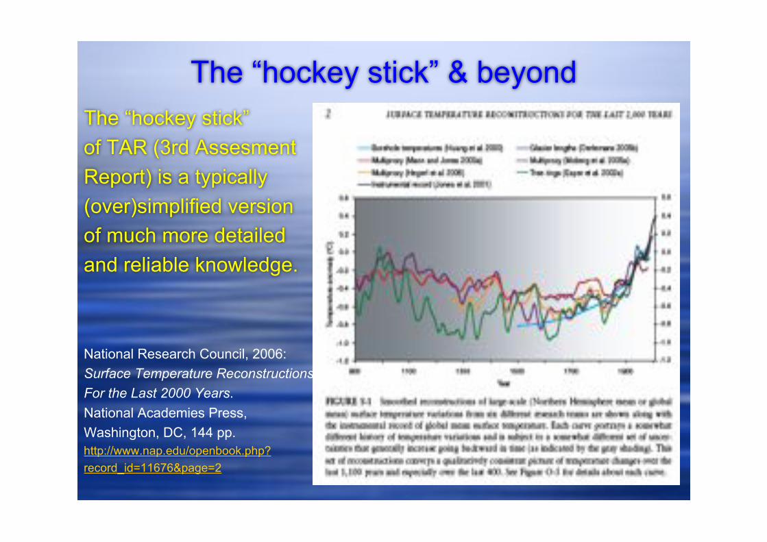
The “hockey stick” & beyond
The “hockey stick”
of TAR (3rd Assesment
Report) is a typically
(over)simplified version
of much more detailed
and reliable knowledge.
National Research Council, 2006:
Surface Temperature Reconstructions
For the Last 2000 Years.
National Academies Press,
Washington, DC, 144 pp.
http://www.nap.edu/openbook.php?
record_id=11676&page=2

D!a
prè
s K
uo
-Nan
Lio
u, 1980:
An
In
tro
du
cti
on
to
Atm
osp
heri
cR
ad
iati
on
(fi
g.
8.1
9)
Bil
an
én
erg
éti
qu
e d
e l"a
tmo
sp
hè
rete
rre
str
e
(4 )
(+2
4)
(+2
2)
(+53)
(+4
5)
(2 4)
(33
)
(+2
1)
(3)
(45
)
(+26)
(+47)
(67
)
(- 30
)(- 3
0)
(+9
8)
(- 11
3)
(30 + 22 = 52)
Va
leu
rs e
n r
ou
ge
: c
f. fi
gu
rep
réc
éd
en
te.
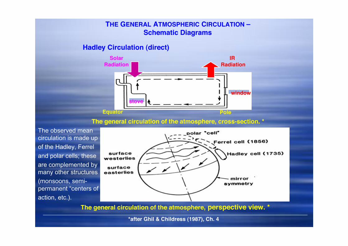
THE GENERAL ATMOSPHERIC CIRCULATION –Schematic Diagrams
Hadley Circulation (direct)
The general circulation of the atmosphere, perspective view. *
The general circulation of the atmosphere, cross-section. *
*after Ghil & Childress (1987), Ch. 4
Equator Pole
Solar Radiation
IR Radiation
stove
window
The observed mean
circulation is made up
of the Hadley, Ferrel
and polar cells; these
are complemented by
many other structures
(monsoons, semi-
permanent “centers of
action, etc.).

Modeling Hierarchy for the Oceans
Ocean models
! 0-D: box models – chemistry (BGC), paleo
! 1-D: vertical (mixed layer, thermocline)
! 2-D – meridional plane – THC " also 2.5-D: a little longitude dependence
– horizontal – wind-driven " also 2.5-D: reduced-gravity models (n.5)
! 3-D: OGCMs - simplified - with bells & whistles (“kitchen sink”)
Coupled 0-A models
! Idealized (0-D & 1-D): intermediate couple models (ICM)
! Hybrid (HCM) - diagnostic/statistical atmosphere
- highly resolved ocean
! Coupled GCM (3-D): CGCM
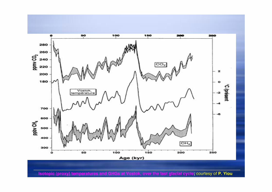
Isotopic (proxy) temperatures and GHGs at Vostok, over the last glacial cycle; courtesy of P. Yiou
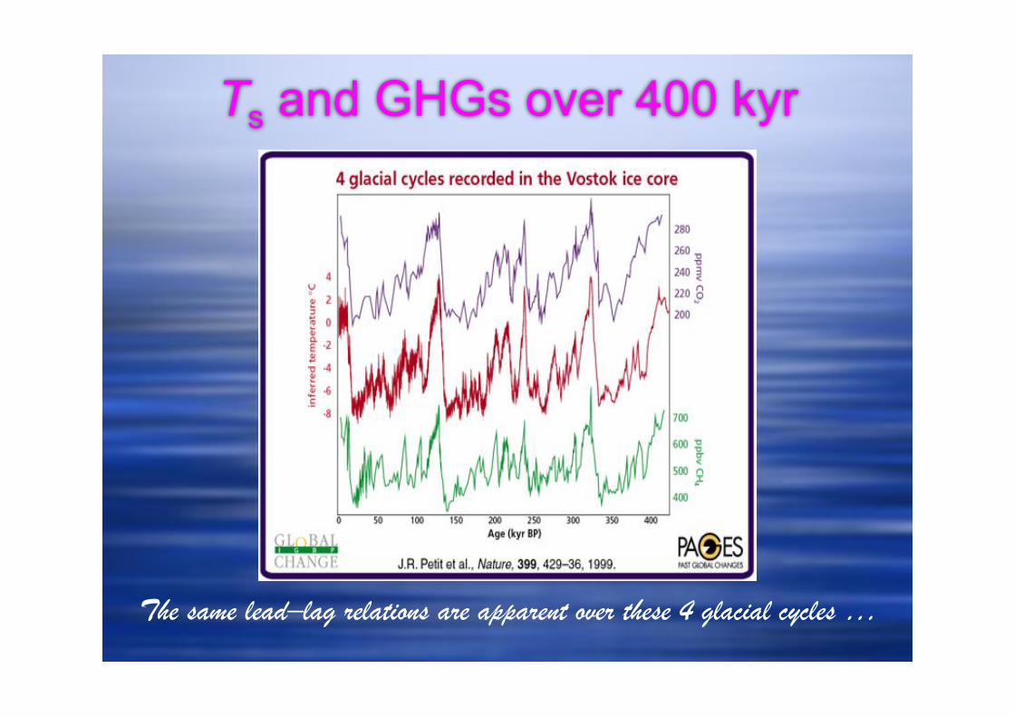
Ts and GHGs over 400 kyr
The same lead–lag relations are apparent over these 4 glacial cycles …
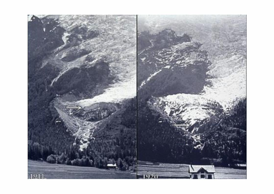
The Glacier des Bossons: 2 photos, 9 years apart
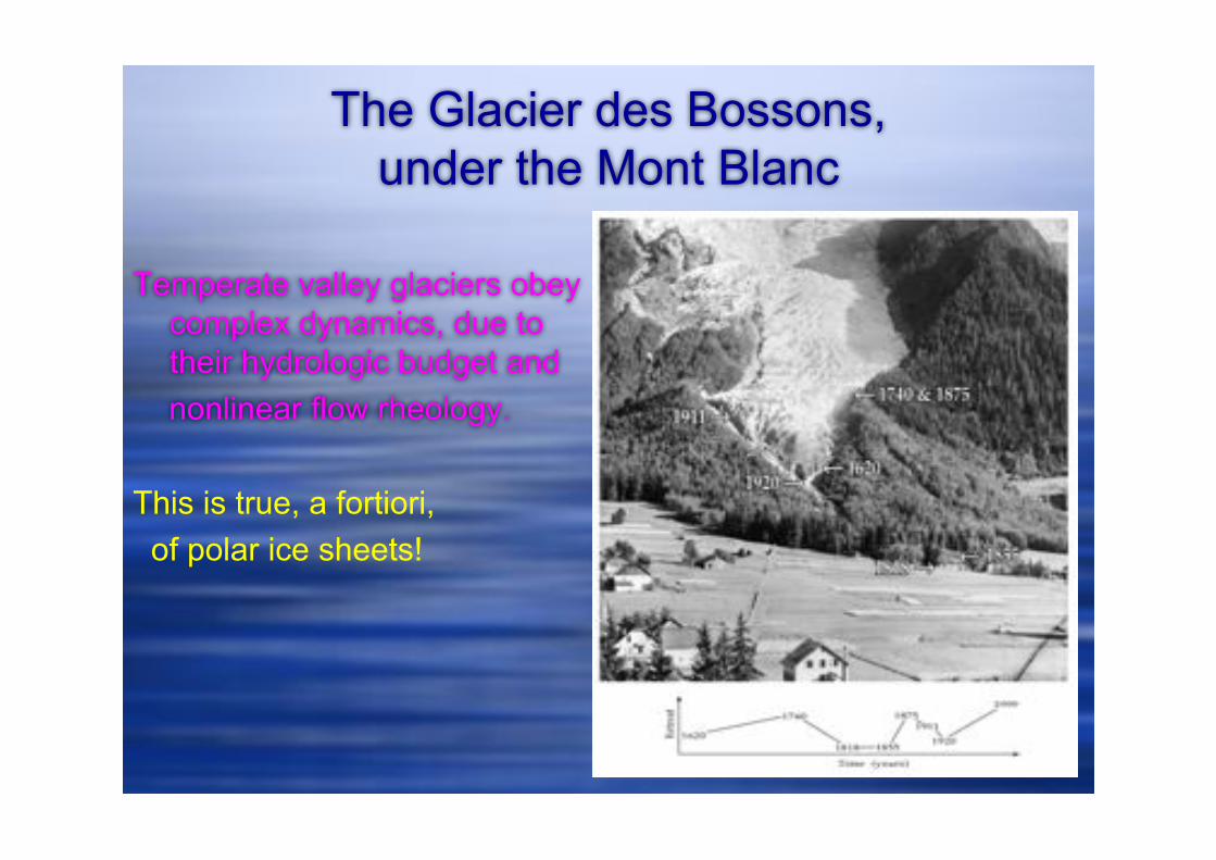
The Glacier des Bossons,
under the Mont Blanc
Temperate valley glaciers obey
complex dynamics, due to
their hydrologic budget and
nonlinear flow rheology.
This is true, a fortiori,
of polar ice sheets!
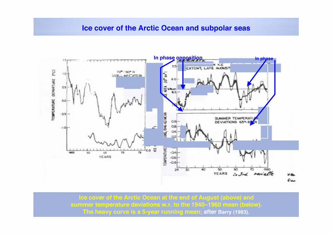
Ice cover of the Arctic Ocean and subpolar seas
Ice cover of the Arctic Ocean at the end of August (above) andsummer temperature deviations w.r. to the 1940–1960 mean (below).
The heavy curve is a 5-year running mean; after Barry (1983).
In phase opposition In phase

Sun-Climate Relations
• It ain!t new:
v. ~1000papers (in1978!), as wellas Marcus et al.(1998, GRL).
• “Corrélationn!est pasraison.”
• Requiresserious study ofsolar physics.

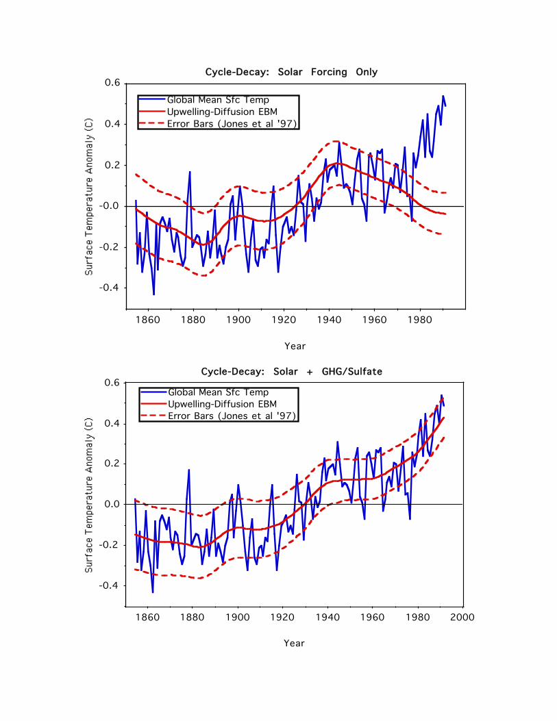
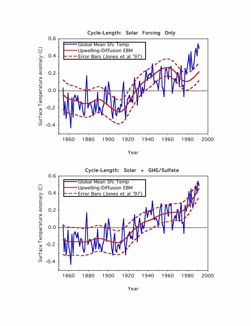
Solar Effects on Interdecadal Climate Variability
Irradiance Anomaly: dw/dt + w/τ = k F(t)
( tm ~ time of solar min.; tM ~ solar max.; τ ~ L2/ν )
1) Cycle-Length (CL) Model: F2(tm+1/2) = k2 / (tm+1-tm)
2) Cyle Decay-Rate (CD) Model: F1(tm) = k1 / (tm-tM)
1850 1900 1950 2000-0.4
-0.2
0.0
0.2
0.4
-0.5
0.0
0.5
1.0
1.5
Year
Decay-Rate Model Cycle-Length Model Anthropogenic Forcing
Climate Model: Global energy-balance model, with upwelling-diffusion ocean model underneath (cf. IPCC)
S. L. Marcus, M. Ghil, and K. Ide, Geophys. Res. Lett., 26 1449-
1452, 1999
1860 1880 1900 1920 1940 1960 1980
-0.4
-0.2
-0.0
0.2
0.4
0.6
Year
Cycle-Decay: Solar Forcing Only
Global Mean Sfc Temp Upwelling-Diffusion EBM Error Bars (Jones et al '97)
1860 1880 1900 1920 1940 1960 1980 2000
-0.4
-0.2
0.0
0.2
0.4
0.6
Year
Cycle-Decay: Solar + GHG/Sulfate
Global Mean Sfc Temp Upwelling-Diffusion EBM Error Bars (Jones et al '97)
1860 1880 1900 1920 1940 1960 1980 2000
-0.4
-0.2
0.0
0.2
0.4
0.6
Year
Cycle-Length: Solar Forcing Only
Global Mean Sfc Temp Upwelling-Diffusion EBM Error Bars (Jones et al '97)
1860 1880 1900 1920 1940 1960 1980 2000
-0.4
-0.2
0.0
0.2
0.4
0.6
Year
Cycle-Length: Solar + GHG/Sulfate
Global Mean Sfc Temp Upwelling-Diffusion EBM Error Bars (Jones et al '97)