3

SAND2004-0076 UNLIMITED RELEASE

PRINTED JUNE 2004

FLUID FLOW MODELING OF RESIN TRANSFER MOLDING FOR COMPOSITE MATERIAL WIND TURBINE

BLADE STRUCTURES

Principal Investigator: Douglas S. Cairns Written by: Scott M. Rossell

Department of Chemical Engineering Montana State University-Bozeman

Bozeman, Montana

ABSTRACT

Resin transfer molding (RTM) is a closed mold process for making composite materials. It has the potential to produce parts more cost effectively than hand lay-up or other methods. However, fluid flow tends to be unpredictable and parts the size of a wind turbine blade are difficult to engineer without some predictive method for resin flow.

There were five goals of this study. The first was to determine permeabilities for three fabrics commonly used for RTM over a useful range of fiber volume fractions. Next, relations to estimate permeabilities in mixed fabric lay-ups were evaluated. Flow in blade substructures was analyzed and compared to predictions. Flow in a full-scale blade was predicted and substructure results were used to validate the accuracy of a full-scale blade prediction.

4

5

TABLE OF CONTENTS

LIST OF FIGURES ............................................................................................................ 9

LIST OF TABLES............................................................................................................ 13

ABSTRACT...................................................................................................................... 16

1. INTRODUCTION ........................................................................................................ 17

Motivation.................................................................................................................... 18 Objective and Approach............................................................................................... 21 Organization of Report................................................................................................. 21

2. BACKGROUND .......................................................................................................... 23

Composite Materials .................................................................................................... 23 Material Properties .................................................................................................. 24 Resin Systems ......................................................................................................... 25 Fiber Reinforcements .............................................................................................. 25

Composite Manufacturing............................................................................................ 26 Hand Lay-up............................................................................................................ 27 RTM ........................................................................................................................ 28

Flow Theory................................................................................................................. 29 Preform Geometry................................................................................................... 30 General Flow ........................................................................................................... 32 Darcy’s Law ............................................................................................................ 33

Permeability Determination ......................................................................................... 35 Numerical Calculation Methods.............................................................................. 35 Experimental Methods ............................................................................................ 37 Sources of Error ...................................................................................................... 40

Modeling Theory.......................................................................................................... 42 Micro Modeling Schemes ....................................................................................... 42

MSU Micro Model ............................................................................................. 43 Macro-Flow Modeling Schemes ............................................................................. 44

LIMS................................................................................................................... 44 Flow Phenomena (Sources for Modeling Error) ..................................................... 45

3. EXPERIMENTAL METHODS AND PROCEDURES............................................... 47

Materials and Process Equipment ................................................................................ 47 E-glass fiber reinforcement ..................................................................................... 47 Resin System ........................................................................................................... 51 Injection Equipment ................................................................................................ 51 Molds....................................................................................................................... 52

Flat plate mold.................................................................................................... 52

6

Thick Flanged T-section Mold ........................................................................... 53 Steel Root Insert Mold........................................................................................ 55

Imaging Equipment ................................................................................................. 55 Resin and Fabric Characterization ............................................................................... 56

Motivation ............................................................................................................... 56 Resin Viscosity........................................................................................................ 56 Surface Tension....................................................................................................... 58 Capillary Pressure ................................................................................................... 59 Experiment Designation Scheme ............................................................................ 60 Fiber Volume Fraction ............................................................................................ 60 Fiber Burn-off ........................................................................................................ 61 Relative Thickness .................................................................................................. 61 Fiber Stacking and Compressibility ........................................................................ 62

Permeability ................................................................................................................. 64 Motivation and Test Matrix..................................................................................... 64 Experimental Methods ............................................................................................ 64

Mixed Fabric ................................................................................................................ 66 Motivation and Test Matrix..................................................................................... 66 Predictive Methods.................................................................................................. 68 Experimental Procedures......................................................................................... 69

T-Section...................................................................................................................... 69 Motivation and Test Matrix..................................................................................... 69 Experimental Methods ............................................................................................ 70

Root Insert Section....................................................................................................... 72 Experimental Procedures......................................................................................... 73

4. EXPERIMENTAL RESULTS...................................................................................... 75

Resin and Fabric Characterization ............................................................................... 75 Viscosity.................................................................................................................. 75 Surface Tension....................................................................................................... 78 Capillary Pressure ................................................................................................... 79 Fiber Volume Fraction ............................................................................................ 80 Fabric Stacking and Compressibility ...................................................................... 81

Permeability ................................................................................................................. 87 A130 Fabric............................................................................................................. 88 DB120 Fabric Results ............................................................................................. 90 D155 Fabric............................................................................................................. 92 Permeability Discussion.......................................................................................... 94

Mixed Fabric ................................................................................................................ 99 Experimental Results............................................................................................... 99 Predictive Data used.............................................................................................. 102 Predictive Results .................................................................................................. 103 Summary ............................................................................................................... 112

T-Section.................................................................................................................... 113

7

TA01...................................................................................................................... 113 TD01...................................................................................................................... 116 TA02...................................................................................................................... 118

Steel Root Insert Mold ............................................................................................... 120

5. NUMERICAL RESULTS AND CORRELATION WITH EXPERIMENTS............ 123

LIMS basics ............................................................................................................... 123 Model Creation...................................................................................................... 123 LIMS input parameters.......................................................................................... 126 Recording information .......................................................................................... 127

Flat Plate models ........................................................................................................ 127 Experimental Error ................................................................................................ 128 A130 08 Lay-up (SA08-1) ..................................................................................... 128 D155 06 Lay-up (SD06-1) ..................................................................................... 130 A130-DB120 [0/±452/0]s Lay-up.......................................................................... 131 A130 [0/90/0/90 ]s Lay-up.................................................................................... 133

T-section Results........................................................................................................ 134 Thick flanged T model .......................................................................................... 134 A130 Center Injected T-mold (TA01) .................................................................. 135 D155 Center Injected T-mold (TD01) .................................................................. 136 A130 End Injected T-mold (TA02)....................................................................... 139

Steel Insert Results..................................................................................................... 141 Insert Model .......................................................................................................... 142 Results ................................................................................................................... 144

Blade Models ............................................................................................................. 145 Model .................................................................................................................... 146 End Injection ......................................................................................................... 146 Multiple Port injection .......................................................................................... 147 Discussion ............................................................................................................. 148

6. RESULTS SUMMARY, RECOMMENDATIONS AND FUTURE WORK ........... 150

Fabric Characterization .............................................................................................. 150 Permeability ............................................................................................................... 150

Single Fabric Permeability .................................................................................... 150 Mixed Fabric Permeability.................................................................................... 151

Modeling .................................................................................................................... 151 Thick Flange T Mold............................................................................................. 151 Steel Insert Mold ................................................................................................... 152 Blade...................................................................................................................... 152

Recommendations...................................................................................................... 152 Future Work ............................................................................................................... 153

REFERENCES CITED................................................................................................... 154

APPENDICES ................................................................................................................ 158

8

APPENDIX A ............................................................................................................ 159 Description of Calculations................................................................................... 160 Mixed Fabric Experiments .................................................................................... 168

APPENDIX B ............................................................................................................ 175 Relative Thickness Example Calculation.............................................................. 176 Clamping Pressure Example Calculation.............................................................. 176

APPENDIX C ............................................................................................................ 178 Key-points along Blade......................................................................................... 179 Lay-up Information and Permeabilities for Blade Model ..................................... 180

9

LIST OF FIGURES Figure 1. AOC 15/50 blade and cross section (length is approximately 8 m). ................ 18

Figure 2. Components of the AOC 15/50. ....................................................................... 19

Figure 3. Rough inside surface of a wind turbine blade. ................................................. 19

Figure 4. Thick bond line in a wind turbine blade........................................................... 20

Figure 5. Cross section of a [0/902/0]s composite. .......................................................... 23

Figure 6. Schematic of the axis relative to a roll of fabric............................................... 26

Figure 7. Diagram of a simple RTM injection setup. ...................................................... 28

Figure 8. Multiple length scales for flow......................................................................... 30

Figure 9. D155 fiber bundle............................................................................................. 31

Figure 10. Common fabrics used for RTM and hand lay-up........................................... 32

Figure 11. Generalized flow for an anisotropic medium with an injection port of radius R0 centered at (0,0). ............................................................................ 38

Figure 12. Stacking sequence for a [+45/0/-45] lay-up. Fibers are the solid regions and channels are void spaces between fibers. ................................... 43

Figure 13. Photograph showing a void area in a T-section.............................................. 46

Figure 14. Three regions of flow in an RTM mold.......................................................... 46

Figure 15. A130 Fabric. ................................................................................................... 48

Figure 16. D155 Fabric ..................................................................................................... 49

Figure 17. DB120 Fabric ................................................................................................. 50

Figure 18. 0° and ±45° sides of CDB200 fabric. ............................................................. 50

Figure 19. Pressure pot. ................................................................................................... 52

Figure 20. Flat plate mold................................................................................................ 53

Figure 21. Schematic of thick flanged T section and its dimensions............................... 54

Figure 22. T-section mold................................................................................................ 54

10

Figure 23. Skin and inner-surface halves of the steel insert mold. .................................. 56

Figure 24. Capillary rheometer. ....................................................................................... 57

Figure 25. Fabric compression diagram........................................................................... 64

Figure 26. Diagram of experimental permeability setup. ................................................ 67

Figure 27. Regions of the AOC 15/50 that may be modeled by a flat plate geometry. ....................................................................................................... 67

Figure 28. T-section part and how it relates to the AOC 15/50....................................... 70

Figure 29. Port locations on the thick flanged T-mold. ................................................... 71

Figure 30. Steel insert part and how it relates to the AOC 15/50. ................................... 73

Figure 31. Lay-up of the skin side of the insert mold...................................................... 74

Figure 32. Viscosity of catalyzed CoRezyn 63-AX-051 with time. The average value for the uncatalyzed resin is shown at time equal to 0. ......................... 76

Figure 33. Comparison of relative thickness method prediction with experimental burn-off results............................................................................................... 81

Figure 34. Displacement of fabric compression test fixture without fabric as a function of load. Error bars are placed on Run 3.......................................... 82

Figure 35. Compressibility of unidirectional A130, DB120 and D155 fabrics. .............. 83

Figure 36. Effects of lay-up on A130 fabric stacking...................................................... 85

Figure 37. Effects of lay-up on D155 fabric stacking...................................................... 86

Figure 38. Effect of mixed fabrics on fiber volume fraction. .......................................... 87

Figure 39. Contour plot for experiment SA08-1. Times are listed in minute_second format on the legend. The lay-up consisted of 8 layers of A130 fabric with a fiber volume fraction of 0.40...................................... 89

Figure 40. A130 unidirectional permeability versus fiber volume fraction..................... 89

Figure 41. Contour plot for experiment SB08-1. Times are listed in minute_second format on the legend. The lay-up consisted of 8 layers of DB120 fabric with a fiber volume fraction of 0.31. .................................. 91

Figure 42. Permeability versus fiber volume fraction for DB120 fabric......................... 92

11

Figure 43. Contour plot for experiment SD06-1. Times are listed in minute_second format on the legend. The lay-up consisted of 6 layers of D155 fabric with a fiber volume fraction of 0.40...................................... 93

Figure 44. D155 permeability versus fiber volume fraction for a unidirectional lay-up. ............................................................................................................ 94

Figure 45. Unsaturated flow occurring in a unidirectional A130 lay-up......................... 95

Figure 46. Permeability variation for three experiments with A130 fabrics. .................. 95

Figure 47. Summary of single fabric permeability data. ................................................. 96

Figure 48. Transverse and longitudinal permeabilities for mixed fabric experiments……………………………………………………….............. 100

Figure 49. Plot of experimental and predicted flow fronts for test MA01-2 at 1800 sec. with an injection pressure of 86.2 kPa......................................... 104

Figure 50. Plot of experimental and predicted flow front positions for test MD01-1 at 500 sec. with an injection pressure of 89.7 kPa.................................... 105

Figure 51. Summary of longitudinal permeability estimates versus experimentally determined permeabilities for the Mx01, Mx02 and Mx03 series lay-ups.......................................................................................................... 107

Figure 52. Summary of transverse permeability predictions versus experimentally determined permeabilities for the Mx01, Mx02 and Mx03 series lay-ups.......................................................................................................... 108

Figure 53. Predicted versus experimental Kx values for the Mx04 and Mx05 lay-ups.......................................................................................................... 110

Figure 54. Predicted versus experimental Ky values for the Mx04 and Mx05 lay-ups.......................................................................................................... 111

Figure 55. Source of high permeability in T-sections.................................................... 115

Figure 56. Flow front positions for TA01. Injection was from two central injection ports (shown as black dots) at a pressure of 82.7 kPa. ................. 116

Figure 57. Flow front positions TD01. Injection was from two central injection ports (shown as black dots) at a pressure of 82.7 kPa. ................................ 118

Figure 58. Flow front positions for TA02. Injection was from two injection ports located at the end of the mold. Injection pressure was at 82.7 kPa. ........... 120

12

Figure 59. Filling pattern of insert mold with an injection pressure of 96.5 kPa. ......... 122

Figure 60. Experimental versus predicted flow front positions for SA08-1, single fabric A130. Kx=9.90x10-11 Ky=3.47x10-11, vf=0.400, µ=0.195 kg/m⋅s and P=89.7 kPa. ........................................................................................... 129

Figure 61. Experimental versus predicted results for SD06-1, single fabric D155. Kx=6.16x10-10 Ky=4.80x10-11, vf=0.398, µ=0.195 kg/m⋅s and P=89.7 kPa. .............................................................................................................. 131

Figure 62. Flow contours comparing the experimentally determined permeability with two predictive methods. Flow front times are at 85 and 1800s from an injection port located at the origin. Quarter symmetry was assumed........................................................................................................ 132

Figure 63. Flow contours comparing the experimentally determined permeability with the relative thickness predictive method for the MA03-2 lay-up (0/90/0/90 )s. Flow front times were at 54 s, 320s and 900 s from an injection port located at the origin. Quarter symmetry was assumed......... 133

Figure 64. Meshed T-mold showing the three different lay-up regions. ....................... 135

Figure 65. Predicted versus experimental results for case TA01................................... 137

Figure 66. Predicted versus experimental results for case TD01.................................... 139

Figure 67. Experimental versus predicted results for TA02. ......................................... 141

Figure 68. Sections of insert model. .............................................................................. 142

Figure 69. Meshed insert model with a close up at the insert tip region. ...................... 143

Figure 70. Insert Model versus experimental results. Injection at 96.5 kPa................. 145

Figure 71. Tip end of AOC 15/50 blade. ....................................................................... 146

Figure 72. End injection of AOC 15/50 blade. View is from the low pressure side of the blade. .......................................................................................... 147

Figure 73. Multi-port injection of AOC 15/50 blade. Six injection ports were located at three locations along the blade length on both the low and high-pressure sides of the blade at the web skin intersection. View is from the low-pressure side of the blade....................................................... 148

13

LIST OF TABLES Table 1. Tensile properties of aluminum, E-glass, polyester resin, and E-glass,

polyester composites...................................................................................... 24

Table 2. Summary of E-glass fabric reinforcement material used................................... 47

Table 3. Rheometer dimensions....................................................................................... 57

Table 4. Viscosity Experiments. ...................................................................................... 59

Table 5. Burn off tests...................................................................................................... 61

Table 6. Fabric stacking and compression test matrix. .................................................... 63

Table 7. Permeability test matrix. .................................................................................... 65

Table 8. Mixed fabric test matrix..................................................................................... 68

Table 9. Properties of T-section components. ................................................................. 72

Table 10. Viscosity Results.............................................................................................. 76

Table 11. Surface tension results. .................................................................................... 79

Table 12. Capillary pressure. ........................................................................................... 80

Table 13. Relative thickness and fabric composition results. Results are an average of three tests performed on each fabric type. ................................... 80

Table 14. Correlations for permeability as a function of fiber volume. ........................ 103

Table 15. Ply thickness versus clamping pressure relationships. .................................. 103

Table 16. Predicted lay-up composition and permeabilities for Mx04 and Mx05 lay-ups.......................................................................................................... 109

Table 17. Comparison of predicted to experimental flow front shapes......................... 112

Table 18. Matrix of mesh sensitivity runs on a 510 mm by 810 mm plate model with quarter symmetry and the injection port located at the origin. ............ 124

Table 19. Mesh sensitivity flow results. ........................................................................ 125

Table 20. LIMS input parameters .................................................................................. 126

14

Table 21. Fabric related LIMS input properties for thick flanged T model TA01. Injection took place at 82.7 kPa from a central injection port and with a resin viscosity of 0.195 kg/m⋅s. ................................................................ 135

Table 22. Fabric related LIMS input properties for thick flanged T model TD01. Injection took place at 82.7 kPa from a central injection port and with a resin viscosity of 0.195 kg/m⋅s. ................................................................ 137

Table 23. Fabric related LIMS input properties for thick flanged T model TA02. Injection took place at 82.7 kPa from an end of the skin. A resin viscosity of 0.195 kg/m⋅s was used. ............................................................ 140

Table 24. Fabric related LIMS input properties for steel insert model. Injection took place at 96.5 kPa with a resin viscosity of 0.195 kg/m⋅s. .................... 143

Table 25. Example of a permeability spread sheet. ....................................................... 161

Table 26. Experiment SA06-1, A130 06. ....................................................................... 161

Table 27. Experiment SA07-1, A130 07. ....................................................................... 162

Table 28. Experiment SA08-1, A130 08. ....................................................................... 162

Table 29. Experiment SA08-2, A130 08. ....................................................................... 163

Table 30. Experiment SA08-3, A130 08. ....................................................................... 163

Table 31. Experiment SA09-1, A130 09. ....................................................................... 164

Table 32. Experiment SB07-1, DB120 07...................................................................... 164

Table 33. Experiment SB08-1, DB120 08...................................................................... 165

Table 34. Experiment SB10-1, DB120 010. ................................................................... 165

Table 35. Experiment SB12-1, DB120 012. ................................................................... 166

Table 36. Experiment SD05-1, D155 05. ....................................................................... 166

Table 37. Experiment SD06-1, D155 06. ....................................................................... 167

Table 38. Experiment SD08-1, D155 08. ....................................................................... 167

Table 39. Experiment SD09-1, D155 09. ....................................................................... 168

Table 40. Experiment MA01-1, A130 [0/902/0]s .......................................................... 168

15

Table 41. Experiment MA01-2, A130 [0/902/0]s .......................................................... 169

Table 42. Experiment MA02-1, A130 [(90/0)2]s........................................................... 169

Table 43. Experiment MA03-1, A130 [0/90/0/90 ]s...................................................... 170

Table 44. Experiment MA03-2, A130 [0/90/0/90 ]s...................................................... 170

Table 45. Experiment MA04-1, A130/DB120 [0/±45/0]s............................................. 171

Table 46. Experiment MA05-1, A130/DB120 [0/±45/90]s........................................... 171

Table 47. Experiment MD01-1, D155 [0/902/0]s. ......................................................... 172

Table 48. Experiment MD02-1, D155 [(90/0)2]s........................................................... 172

Table 49. Experiment MD03-2, D155 [0/90/0/90 ]s...................................................... 173

Table 50. Experiment MD04-1, D155/DB120 [0/±452/0]s. .......................................... 173

Table 51. Experiment MD04-1, D155/DB120 [0/±452/90]s. ........................................ 174

Table 52. Key-points for blade model. .......................................................................... 179

Table 53. Permeabilities along blade section................................................................. 180

16

FULL ABSTRACT

Resin transfer molding (RTM) is a closed mold process for making composite materials. It has the potential to produce parts more cost effectively than hand lay-up or other methods. However, fluid flow tends to be unpredictable and parts the size of a wind turbine blade are difficult to engineer without some predictive method for resin flow.

There were five goals of this study. The first was to determine permeabilities for three fabrics commonly used for RTM over a useful range of fiber volume fractions. Next, relations to estimate permeabilities in mixed fabric lay-ups were evaluated. Flow in blade substructures was to be analyzed and compared to predictions. Flow in a full-scale blade was to be predicted and substructure results were to be used to validate the accuracy of a full-scale blade prediction.

Permeabilities were calculated for three fabrics (A130, DB120 and D155) in the fiber volume fraction range of 0.27 to 0.47. In addition, relationships were determined for each fabric over the given range of fiber volume fractions.

Two estimation methods were used to predict flow. One method was based on the relative thickness of glass in the fabrics and the other was based on the thickness of fabric layers at a given clamping pressure. The clamping pressure method was able to accurately predict the flow front shapes of a lay-up, but tended to under predict permeabilities. The relative thickness method did not capture the proper flow front shapes and under predicted permeabilities as well.

Liquid Injection Modeling Simulation (LIMS) was used to predict flow in the substructural models. Substructures in which flow was analyzed include a thick flanged T-section and a steel root insert. Filling times were well predicted in the T-section, but flow front shapes were not exact due to preferential flow in the mold. The steel root insert section was not well predicted due to the complex lay-up and a significant amount of interlaminar flow.

Two full blade simulations were created. One was an end injection and the other consisted of 6 injection ports in three stations. Ports were located at the flange on the low and high pressure sides of the blade at each station. Filling times were reduced by a factor of 10 using the 3 stage injection instead of injection from an end.

Based on results from the substructure experiments, the blade filling times are overpredicted. Due to the large scale of the blade, interlaminar flow problems should be negligible so flow front shapes should be accurately predicted.

17

CHAPTER 1

INTRODUCTION

Advanced composite materials offer an exciting and diverse alternative to

traditional materials. Their high strength and stiffness-to-weight ratios combined with a

wide range of design options have allowed them to be a popular material in performance-

driven areas such as aerospace and sporting goods industries. In addition, they can

provide a competitive, low-cost solution in piping, storage tank, and marine

applications.1, 2 Another application where advanced composites are gaining popularity

is the wind industry. E-glass reinforced polyester, vinyl-ester and epoxy composites are

the materials of choice for producing wind turbine blades. These composites allow

designers to make lighter more efficient blades at an affordable price.

Wind energy is a clean, renewable source of energy. Despite the potential

benefits of wind energy, its cost per kilowatt-hour remains high enough to limit its

growth in the United States. One area where wind energy can see a cost reduction is in

the manufacturing of wind turbine blades. Currently most composite wind turbine blades

are manufactured by the hand lay-up process. The blade for the AOC 15/50 wind turbine

is one example.3 Resin transfer molding (RTM) offers the potential of making lighter,

more efficient blades while at the same time lowering production costs of the blades.4 5

A typical blade geometry and structure are illustrated in Figure 1.3

18

Figure 1. AOC 15/50 blade and cross section (length is approximately 8 m).3

Motivation

Hand lay-up involves manufacturing by the sequential addition of layers of

reinforcement and resin matrix in an open mold. It allows for the manufacture of a wide

range of geometries and requires low initial investment. Despite these advantages, hand

lay-up is not well suited to large-scale production due to the fact that it is very labor

intensive and requires long cycle times. In addition, it is not easy to make hollow

structures with the hand lay-up process. Therefore, a blade is usually manufactured in

pieces and secondarily bonded together, Figure 2. The hand lay-up process uses a one-

sided mold, which adds complications to the manufacturing process. For example, parts

tend to vary significantly in thickness and only have only one finished surface. The

unfinished surface requires additional time to condition for bonding, Figure 3, and poor

manufacturing tolerances may result in thick and/or thin bond lines, Figure 4. Another

19

limitation of hand lay-up, is that fiber volume fractions are generally under 35%4. Since

the fibers bear the majority of the load in a composite, the presence of excess resin just

adds weight. A weight savings of 6.3 kg, 10% of the AOC 15/50 blade weight, would be

achieved if the skin thickness could be compressed by one millimeter.4

Figure 2. Components of the AOC 15/50 wind turbine blade.

Figure 3. Rough inside surface of a wind turbine blade.

20

Figure 4. Thick bond line in a wind turbine blade

Resin Transfer Molding (RTM) offers numerous advantages over hand lay-up.4

Parts can be produced more rapidly with less labor expense. In addition, it is possible to

more easily produce hollow parts with RTM since all fiber layers are placed into a two-

sided mold before resin is added. This reduces the labor required to make a part. Also,

the two-sided mold produces parts with tighter dimensional tolerances, higher fiber

volume fractions and a smooth surface finish on all surfaces. RTM also eliminates

excess resin and thick bond lines. Thus, even if the blade is molded in parts the weight is

lowered and parts are much easier to condition for secondary bonding.

Fabricating RTM molds are much more expensive to make than ones for hand

lay-up, thus hindering their development. Multiple injection ports may be necessary for

parts on the scale of wind turbine blades to keep injection times under the gel time of the

resin. This complicates flow patterns and may result in a mold that traps air, creating dry

spots, or ones that fill incompletely. Currently, mold design is more of an art than a

science; the odds that the initial layout of injection ports will have problems appear to be

high. Since molds are very costly, accurate prediction of resin flow in the mold is

21

desirable. There has been a great deal of research in flow modeling for RTM. However,

much of the research has not addressed the types of fiber reinforcements that are of

interest for wind turbine blades, or has involved micro-flow models that would not be

practical to model parts the size of a blade.

Objective and Approach

The objective of this research was to compare experimental resin flow modeling

results for small-scale substructural components of the AOC 15/50 blade with predictions

from generalized flow modeling software. Models were refined to better predict the resin

flow observed in the substructural components. The models were then applied to predict

the flow in larger, full-scale blades. Specific project goals were as follows:

1) Experimentally determine permeabilities for reinforcing fabrics of interest (A130, D155 and DB120) at different fiber volume fractions

2) Determine the accuracy with which permeabilities for individual fabrics can be used to predict permabilities for mixed and single fabric lay-ups.

3) Simulate flow in blade substructures using permeability data as input for flow prediction modeling software Liquid Injection Modeling Simulation (LIMS) and compare the flow predictions with experimental data.

4) Use LIMS to predict resin flow in a wind turbine blade

5) Use substructure prediction versus experimental correlations to assess the accuracy of a full-scale blade injection

Organization of Report

In Chapter 2, fluid flow theory is described as it relates to modeling flow of the

RTM process. Several modeling methods are also discussed. In Chapter 3, experimental

procedures are discussed and a test matrix is presented. In Chapter 4, all experimental

22

results are presented. In Chapter 5, predictions are compared with experimental results

for resin flow in various geometries, including the full size AOC 15/50 blade. In chapter

6, the conclusions from this study are presented as well as a list of items that should be

included in future studies.

23

CHAPTER 2

BACKGROUND

Composite Materials

Composite materials, by definition, are made from combining two or more

different materials. These materials can be as simple as straw and clay, or as complex as

carbon fiber and epoxy resin. A typical composite material consists of strong, light fibers

held in-place by a polymeric matrix material, Figure 5. E-glass fibers in polyester,

vinyl-ester or epoxy resin are currently the composite materials of choice for wind

turbine blades because of their strength and stiffness to weight ratios, environmental

resistance, and low cost.6, 7

Figure 5. Cross section of a [0/902/0]s composite.

24

Material Properties

Mechanical properties for polyester and E-glass as well as their composites are

given in Table 1. Properties of 6061-T6 aluminum are listed as a reference. One can see

in Table 1 that the E-glass fibers are considerably stronger than the polyester matrix

material. The fibers serve as the primary load bearing material in the composite. The

role of the matrix is to hold the composite together. It also protects the fibers from the

environment and helps distribute loads between fibers. Generally, the composite with the

higher volume fraction of glass fibers will be stronger if all other things are equal. Also,

the strength of a composite is highly dependent on the orientation of the fibers to the

direction of load. The composites are much stronger in the fiber direction, Table 1. This

allows designers to optimize the weight of a structure by reinforcing it in the directions of

anticipated load.

Table 1. Tensile properties of aluminum, E-glass, polyester resin, and E-glass, polyester composites.

Material Tensile Strength (MPa)

Elastic Modulus

(GPa)

Specific Gravity

Strength to Weight Ratio

(103 m) *

Modulus to Weight Ratio

(106 m) * 6061-T6 Aluminum ** 310 68.9 2.70 11.7 2.60 E-glass fibers ** 3450 72.4 2.54 139 2.91 Polyester Resin 3 54.1 3.18 1.16 4.76 0.280 E-glass/polyester [0]8 # 868 36.3 1.78 49.7 2.08 E-glass/polyester [90]8 # 33.8 8.76 1.78 1.94 0.502

* Calculated by dividing the property by its specific weight (density*gravitational acceleration).

** Properities from Reference.2 # Properties from the DOE/MSU database.8 Unidirectional composites with A130 fabric

45% fiber volume tested in the 0° and 90° directions relative to the fiber axis. [0]8 refers to eight fabric layers in the 0° direction.

25

Resin Systems

Common resin systems used in advanced composites include polyesters, vinyl-

esters, epoxies and thermoplastics. Epoxy resin systems tend to be the most versatile, but

are expensive and have environmental concerns associated with them. Thermoplastic

resin systems are the toughest of the resin systems, but they are highly viscous and are

not suited to processing by either hand lay-up or RTM. Polyester and vinyl-ester resins

have low viscosities, are more benign environmentally than epoxies and tend to be the

least expensive. Epoxies, vinyl-esters and polyesters are all commonly used in wind

turbine blade manufacture.

Generally, resin systems are processed as liquids. Resin systems cure by either

forming cross-linked polymer chains, thermosets, or by making very long, entangled

polymer chains, thermoplastics.9 Epoxy, polyester and vinyl-ester resins fall into the

thermoset category. The cure time of a resin system is very important to both RTM and

hand lay-up. Resin systems have to remain liquid long enough to fill the mold and

properly wet out the fibers. The working time of a resin is referred to as the gel time.

Gel times of fifteen minutes to one hour are common for most systems used for both

RTM and hand lay-up.

Fiber Reinforcements

As stated earlier, fibers bear the majority of the load in a composite. Since cost is

a major driving factor in manufacturing wind turbine blades, E-glass fibers are used.

Fibers used for this study were manufactured by Owens Corning and come pre-coated

with a silane coupling agent. The silane provides an environmentally resistant bonding

26

interface so the matrix material bonds with the glass fibers and promotes wetting of the

resin at the fiber surface.

Fibers used for RTM and hand lay-up generally come in a textile form. First,

groups of fibers are bundled together, commonly called fiber tows. Then bundles are

stitched or woven to make a fabric. Fabrics may consist of randomly oriented fibers,

unidirectional fibers or several differently oriented fiber layers stitched together. Fibers

may be orientated in either the weft, or warp direction of the fabric roll, Figure 6. The

most common orientations of fibers are 0°, ±45° and 90°. Many fabrics consist of several

layers stitched together. Weaves of 0° and 90° fibers are also common. While popular in

non-structural applications, random fiber mats are generally used in blades only to hold

the main fibers in place during handling.

Composite Manufacturing

In order to make a composite material, the resin system needs to be combined

with the fiber reinforcement. Since the orientation of the fibers is critical to the

properties, it is essential that the manufacturing process properly align the fibers. In

Figure 6. Schematic of the axis relative to a roll of fabric.

27

addition, a good process will leave parts with a high, uniform fiber volume fraction,

allow rapid production of a large volume of parts economically and have repeatable

dimensional tolerances. The following section describes hand lay-up, the most common

process for manufacturing wind turbine blades, and RTM, a potential process for

improving blade manufacturing.

Hand Lay-up

Hand lay-up is an open mold process. Fabric layers are laid one at a time onto a

one-sided mold. Resin is applied to each layer by pouring or spraying, and pressed

through the thickness with a roller. A squeegee is used to remove excess resin, and then

another layer is added. This process is repeated until all reinforcement layers have been

placed.

Because hand lay-up only requires simple tools and one mold surface, it is

inexpensive to start up. Unfortunately, it also requires a large amount of labor and high

cycle times to produce parts. In addition, the quality of parts manufactured from hand

lay-up tends to be inferior to parts produced by other processing methods.

The fiber placement and impregnation process results in a considerable amount of

fabric handling which may displace fibers. Part thickness depends on the amount of resin

added and is highly variable. High fiber volume fractions are not possible since there is

not another mold face to compress the part. In addition, molds with steep sides may pose

difficulty if the resin viscosity is too low, and hollow parts are difficult to produce with

good dimensional tolerances.4, 10 Another limitation is that parts are only finished on the

mold side. Finally, since hand lay-up is an open mold process, a considerable amount of

28

volatiles are released from the resin during processing.

The shortcomings of hand lay-up result in unnecessary blade weight as well as

extra time processing and assembling blade parts, and exposure of workers to volatile

resin components. Each of these areas can be improved by RTM.

RTM

RTM is a closed mold process. First, dry reinforcing fibers are placed in a two-

sided mold. The mold is then sealed, and at this time, it is common to pull a vacuum. A

vacuum helps eliminate void formation during injection since the resin does not need to

push air out of the mold. The resin is then mixed to initiate curing and injected under

pressure. For a diagram of a typical RTM injection see Figure 7.

Figure 7. Diagram of a simple RTM injection setup.

29

Resin viscosity is critical to the RTM process. Injection times are limited and the

fiber mats have a very low permeability. If pressures get too high, the fibers will be

moved by the resin, commonly called fiber wash. Low viscosities decrease injection

times and lower the risk of fiber wash. It is possible to process resins with viscosities up

to 1000 cP. In practice, however, most RTM resin systems have viscosities less than 500

cP, with ideal resin viscosities in the 100 to 200 cP range.11

The closed mold of RTM offers several advantages over hand lay-up. Parts have

tighter tolerances, they are finished on both sides, and higher fiber volume fractions are

possible. In addition, the reinforcing fiber layers may be preformed so they can be laid

into the mold in one piece, offering considerable time savings. Even without preforming

the fabric, RTM offers a timesaving over hand lay-up in the production of complex

parts.4, 11 In addition, the closed mold prevents volatiles from escaping during

processing. The principal drawback to RTM is the start-up cost. RTM requires

expensive injection equipment, and RTM molds are expensive to produce. Most mold

design and particularly the number and locations of injection and vent ports, is done by

trial and error, and currently it is more of an art than a science. Accurate predictions of

resin flow are necessary in order to properly locate injection and vent ports.

Flow Theory

Prediction of the flow of resin through different mold geometries first requires an

understanding of the fiber mats inside the mold and the processing parameters. Flow

through fibrous preforms tends to be complicated to model. Since the flow is anisotropic,

models must include layer orientation and stacking order as well as the fiber packing

30

density. This section first details the geometric considerations of orientated fiber mats,

and then presents typical methods for describing fluid flow through fibrous media.

Preform Geometry

In order to select an appropriate equation for flow modeling, one must first have a

firm understanding of the micro and macro-geometric details of the reinforcement. There

are multiple length scales in a typical composite, see Figure 8. There are the microscopic

spaces between individual fibers in a fiber tow, spaces on the order of a few millimeters

between fiber tows, and there is the macro geometry of the entire mold.

The smallest micro-geometry exists within the fiber tows as shown in Figure 9.

Typical tows consist of 500 to 3000 fibers grouped together.12 Their permeability is

highly anisotropic, with permeabilities being much higher in the direction of the fibers.

The next level of micro geometry would be the spaces between fiber tows. Finally, there

is the macro geometry of the fabric. Fiber tows are typically formatted into a textile form

for ease of handling since placing fiber tows one at a time into a mold would be

Figure 8. Multiple length scales for flow.

31

impractical. Three common fabrics are D155, A130 and DB120, produced by Owens

Corning Fabrics. The D155 fabric consists of unidirectional fiber tows stitched together,

the A130 fabric consists of unidirectional tows woven over a small glass strand and the

DB120 fabric consists of tows stitched together at a ±45° angle relative to the fabric, see

Figure 10. In addition, tows may be woven over each other in a 0-90° pattern (woven

roving) or tows woven in a satin weave pattern.2 Fiber mats also come in random mat

form and three-dimensional weave patterns, but these are not used widely in blades. The

final complication to fiber preform geometry comes when fiber mats are stacked on top

of one another in differing orientations and compressed when the mold is closed.

Obviously there are numerous ways to incorporate these geometric complexities

into a flow model. Some of the most common approaches are described below.

Figure 9. D155 fiber bundle.

32

Figure 10. Common fabrics used for RTM and hand lay-up.

General Flow

The basic equations for flow of the liquid resin through the spaces in the mats are

described in this section. Generally, resin systems are modeled as Newtonian fluids with

constant density and viscosity so the Navier-Stokes equation is valid.

1) uguDtDu ∇+Ρ∇=+∇+Ρ−∇= 22 µρµρ

where ρ is the density, u is the velocity of the fluid, t is time, P is the pressure, µ is the

viscosity of resin and g is the acceleration due to gravity13.

The generalized Navier-Stokes equation may be further simplified by eliminating

non-linear momentum effects contained in the material derivative. Flow rates in RTM

are slow enough that these effects do not arise.11 The resulting flow type is described as

Stokes flow.

2) u∇+Ρ−∇= 20 µ

The analytical solution of this equation is limited, however. In order to evaluate

the Stokes equation, it is necessary to define fluid velocities or fluxes at the boundaries.

33

Since the resin is flowing through a very complex geometry, evaluating this equation

with its boundary condition would be prohibitively complex. Therefore either the

geometry must be greatly simplified, or a different set of field equations must be

developed.

Darcy’s Law

The most widely used equation for describing flow through RTM molds is

Darcy’s equation for flow through porous media11, a further simplification of Equation 2,

3) ( )iij

i PK

u ∇⋅⎟⎟⎠

⎞⎜⎜⎝

⎛−=

µ

where ui is the volume average velocity of the fluid, Kij is the permeability tensor for the

preform, µ is the viscosity of the resin and P is the pressure in the resin. It is important to

note that Kij is a second order, symmetric tensor. If one were to expand the equation for

three-dimensional flow it would read as follows:

4)

⎪⎪⎭

⎪⎪⎬

⎫

⎪⎪⎩

⎪⎪⎨

⎧

∂∂

∂∂

∂∂

⎟⎟⎟

⎠

⎞

⎜⎜⎜

⎝

⎛

−=⎪⎭

⎪⎬

⎫

⎪⎩

⎪⎨

⎧

zP

yP

xP

KKKKKKKKK

uuu

zzzyzx

yzyyyx

xzxyxx

z

y

x

µ1

Darcy’s law eliminates the need to evaluate complicated boundary equations that arise if

Stokes flow is used, but it requires the evaluation of the permeability tensor. Calculation

of permeabilities is critical to modeling associated with RTM and will be discussed in a

later section.

Darcy’s law has its limitations, which will be discussed, but in nearly all cases it

will apply to flow in RTM molds.11 First, fluid flows need to be within a “seepage”

34

velocity range. In order for the flow to be within this range, the Reynolds number,

Equation 5, must be inversely proportional to the friction factor, Equation 6, of the

medium14.

5) µρδqN =Re

6) ρ

δλ 2

2q

P∆=

where NRe is the Reynolds number, q is the scalar “filter velocity” of the fluid, λ is the

friction factor, ∆P is a one-dimensional pressure drop and δ is a diameter associated to

the flow channels of the preform. A common assumption is that if NRe is one or less then

it is in range of Darcy’s law.11

Another limitation of Darcy’s law is that permeabilities for gases in a porous

medium are higher than those observed for liquids. It has been determined that as the

channel diameter approaches the mean free molecular path of the gas, Darcy’s law breaks

down.15 This can create a problem taking into account pushing air out of a mold that is

not under vacuum.

Also, variations from Darcy’s law have been observed around packed tubes; the

variations were determined to be caused by a boundary effect.14 Flows were found to

increase with distance from the center of the tube, and then drop significantly,

approximately one tube diameter from the wall16.

Finally, fluids modeled by Darcy’s law must obey the assumptions used to

formulate the Navier-Stokes equation. Namely, fluids must have a constant density and

viscosity and must obey Newtonian behavior.

35

Permeability Determination

In order to solve Darcy’s law, one needs to calculate permeabilities. This topic

has been an area of much research in other fields as well as research that directly applies

to RTM. In fact, permeability data have been deemed important enough to the

manufacture of composites that research has been sponsored by the National Institute of

Standards, NIST, to develop a database of fabric permeabilities.17, 18 Additional work has

been done to define a standard reference fabric to assist in the measurement of

permeability.19

Various methods for calculating permeability exist. Both numerical and

experimental models will be discussed in the following section. When modeling flow, it

is common to assume that it occurs in two dimensions since the thickness of parts is

typically small when compared to the other dimensions. Therefore, the calculation

methods detailed below are only for flow in the principal directions of the fabric unless

otherwise noted. This reduces the size of Kij in Equation 4 to a 2-D tensor with three

independent terms.

Numerical Calculation Methods

There are two common ways to calculate permeability values numerically.

Boundary conditions may be defined over a unit cell and the Stokes equation solved, or

hydraulic radius theory may be used to estimate the permeability. The two approaches

are briefly discussed below.

The first approach requires an idealized unit cell. The unit cell must be

representative of the geometry of the fabric being modeled in order to be of practical use.

36

There have been numerous studies in this area.20,21,22,23,24,25 One study was able to

evaluate a unit cell for a woven fabric.20 This was also extended to cover permeabilities

for multi-layer preforms. Evaluating permeabilities this way requires a considerable

amount of time to develop the models, and they contain considerable simplifications of

the fabric geometry. The advantage of this method is it requires no experimental data and

can be quite accurate if the fabric geometry is simple to model.

The Kozeny-Carman equation is a second common method to estimate

permeabilities. The Kozeny-Carman equation (hydraulic radius theory), Equation 7, is

based on taking a volume averaged flow through a porous medium formed from constant

diameter fibers with uniform spacing with a certain volume fraction of connected void

space or connected porosity, on flow channels.

7) ( ) µε

ε Pc

Ru ∆⋅

−= 2

32

1

where u is the volume average velocity, R is the radius of a fiber, ε is the porosity, and c

is a shape factor. The shape factor or tortuosity, c, relating to fibers is dependant on the

arrangement of fibers as well as their packing density.26

The Kozeny-Carman equation is derived from the flow through multiple capillary

tubes which is described by the Hagen-Poiseuille equation26. The Kozeny-Carman

equation is related to Darcy’s law through Equation 8.

8) ( )

2

32 1

f

f

v

vc

RK−

⋅=

where K is the permeability constant and vf is the fiber volume fraction. 27 Therefore, if

the arrangement of fibers is known, the permeabilities may be calculated directly.

37

However, that requires knowing the exact geometry of the fiber structure. So, in practice,

the constants are evaluated experimentally.

The Kozeny-Carman equation works well for isotropic porous media and in cases

of one-dimensional flow, but it has been found to break down in anisotropic fluid

flow.22,23 Obviously, this would be of little use in composites since the oriented fibers

create an anisotropic medium. However, it is possible to modify the Kozeny-Carmen

equation for flow transverse to the fibers.27 In Reference 27 the author used separate

relations for flow parallel and perpendicular to the fibers, and then estimated shape

factors. This approach is limited in its use because it requires fibers that are regularly

aligned, and experimental work is also required. Therefore the preferred method of

determining permeabilities is experimental.

Experimental Methods

There are several methods that one may use to experimentally determine

permeabilities. The two main classes of experiments are saturated and unsaturated. In

saturated flow experiments, the mold (with dry fiber preplaced) is filled until it is

completely saturated with a fluid before measuring flow rates. This approach requires

separate experiments for fabrics orientated at three differing angles in order to calculate

the permeability tensor. Saturated flow experiments accurately characterize

permeabilities, but they require multiple experiments to calculate the permeability tensor.

If one performs an unsaturated experiment with a central injection port, it is possible to

calculate permeabilities with only one experiment as flow may be tracked in both x, y

directions at the same time.28,29

38

A generalized flow front for an unsaturated radial flow experiment is shown in

Figure 11, where Ro is the radius of hole cut into the fabric, R1 and R2 are the radii in the

major and minor flow directions of the fabric and θ is the angle between the fabric

coordinate system and global x and y coordinates. By substitution of Darcy’s law into

the continuity equation, Equation 9, the following expression, Equation 10, is obtained.

9) 0=⋅∇ u

10) ( ) 0=∇⋅⋅∇ pk

If Equation 10 is to be solved for permeabilities, experiments must then be run at a

constant pressure or constant flow rate. The constant pressure method is detailed below.

Information on calculating permeabilities from constant flow rate experiments as well as

saturated flow is detailed by Lai.29

First the location of the flow front must be defined by Equation 11

x

y

θ

R0

R1

R2

Figure 11. Generalized flow for an anisotropic medium with an injection port of radius R0 centered at (0,0).

39

11) flowflow

flowu

dtdxu ⎟

⎠⎞

⎜⎝⎛=⎟

⎠⎞

⎜⎝⎛=

ε

where uflow is the volume averaged velocity of the fluid. If the flow experiment is

performed in the coordinates of the fabric, θ will be zero, eliminating the coupling terms

in the permeability tensor, leaving the following to be solved

12) 02

2

2

2

=∂∂

+∂∂

ypK

xpK yx

In order to solve Equation 12, it must first be transformed into an “equivalent isotropic

system” (EIS)30. The relevant relationships between a point (x,y) and its equivalent in

EIS coordinates (xe, ye) are

13) xox

yexo R

KK

R4

1

, ⎟⎟⎠

⎞⎜⎜⎝

⎛= ; x

x

yy R

KK

R2

1

⎟⎟⎠

⎞⎜⎜⎝

⎛= ; x

x

yxe R

KK

R4

1

⎟⎟⎠

⎞⎜⎜⎝

⎛= ; ( ) 2

1yxe KKK =

where Rx is the radius of the flow front in the x direction, Ry is the radius of the flow front

in the y direction and Rxo is radius of the hole in the fabric. Substitution of these

parameters into Equation 12 leaves a Laplace equation. Solving this equation for the

geometry described earlier gives the following relationship for a volume averaged flow

velocity:31

14) tR

PKRR

RRu

exo

e

exo

xe

exo

xeflow 2

,,

2

,

411ln2εµ

∆=+

⎥⎥⎦

⎤

⎢⎢⎣

⎡−⎟

⎟⎠

⎞⎜⎜⎝

⎛⋅⎟

⎟⎠

⎞⎜⎜⎝

⎛=

Proper substitutions with Equations 13 and 14 yield the following two equations:

15) tR

PKRR

RR

xo

x

xo

x

xo

x2

2411ln2

εµ∆

=+⎥⎦

⎤⎢⎣

⎡−⎟⎟

⎠

⎞⎜⎜⎝

⎛⋅⎟⎟

⎠

⎞⎜⎜⎝

⎛

40

16) yx

xy K

KRR

22 =

Equations 15 and 16 follow linear behavior along principal directions of permeability.

The slopes will be Kx and Ky if the known constants are grouped with their respective

independent variables.

Sources of Error

There are several factors to be considered when preparing permeability experiments.

First, it is of utmost importance that pressure induced mold deflections are kept to a

minimum. Mold deflections will create a part with non-uniform thickness that can alter

preform geometry enough to invalidate the experiments. Two-dimensional unsaturated

flow experiments are most susceptible to this type of error since larger molds with more

surface area, and thus more out-of-plane loads are generated on the mold.

Capillary pressure is another source of error that needs to be taken into account

for unsaturated flow experiments. Under certain conditions capillary forces may be

significant relative to the overall pressure drop of the mold. If so, ∆P of the mold is

described by Equation 17,

17) capoutin PPPP −−=∆

where ∆P is the pressure drop across the mold, Pin is the pressure at the injection port,

Pout is the pressure at the vent and Pcap is capillary pressure.

Capillary pressure is defined by Equation 18,

18) δ

θγ cos=capP

41

where γ is the surface tension of the fluid, θ is the contact angle between the resin and the

fibers and δ is the equivalent diameter of the pores.

It has been observed that this method tends to overpredict capillary pressure in

fibrous preforms.29,32, 33 An alternate method of calculating capillary pressure has been

proposed, Equation 19, based on the Kozeny-Carman equation:32

19) cideal

cap rccP θγ cos2

⋅=

where c is a shape factor based on Kozeny theory, cideal is a correction factor for flow

through an idealized porous media and rc is given by Equation 20

20) ( )επ

ε

−=

12rrc

where r is the radius of an individual fiber and ε is the porosity. This set of equations

takes into account both parallel and serial nonuniformities that are specific to RTM

molds. In addition, they include experimentally determined values for c for a variety of

fabric structures.

Another problem that can arise during one-dimensional flow experiments is

preferential flow. This happens when the fabric is not properly fitted to the mold, leaving

areas of high permeability at the borders, also know as race tracking. If a saturated flow

experiment is run on a mold that exhibits race tracking, it will not measure the true

permeability of the reinforcement.

42

Modeling Theory

Fluid flow in RTM molds is very complex. One complication involves the

treatment of multiphase fluid flow. Prior to injection there is air, or void space if a

vacuum is drawn, and solid fibers. During injection there are multiple flow areas with

resin and fibers in one region and fibers and air or void space in another. Often times a

transition region exists between the two where air and resin coexist in varying

concentrations. Another complication involves dealing with the multiple length scales

present in the fiber preform.

A model that includes all the geometric complexities of the porous medium inside

the mold would be overwhelming for a reasonable sized mold, let alone take into account

the multi-phase flow regions. Thus it is common to make several assumptions when

evaluating flow through RTM molds.

There are two common approaches. The first approach is to combine porous

media theory with more generalized flow models such as Stokes flow to take into account

micro-geometric effects. This approach is referred to as micro-modeling. Another

approach is to use porous media theory and apply it to the entire mold, macro-flow.

Micro-flow models can take into account complex geometry regions of a mold, while

macro-flow models can consider larger, more complex molds.

Micro Modeling Schemes

Micro flow models are important in determining flow in detailed regions of

composites as well as providing a basic understanding of flow in an RTM mold. One

such micro-model was developed at MSU.25,34

43

The model separates flow into two regions, channels and fiber tows. Channel

permeabilities in all three directions are calculated from general flow equations.

Permeabilities along the length of fiber tows are calculated experimentally and

permeabilities transverse to the fiber bundles are calculated using the Kozeny-Carmen

equation, Equation 7, for estimating permeabilities.

Different cells corresponding to either fibers or channels are then stacked

according to the preform geometry, Figure 12. Flow through the cells is solved using the

Gauss-Seidel difference scheme.35 The Gauss-Seidel method was chosen because

pressure at given cells needs to be calculated for every time step in order to advance flow

fronts, and other finite difference methods would not be able to solve for flow in a

reasonable amount of time.

MSU Micro Model

Figure 12. Stacking sequence for a [+45/0/-45] lay-up. Fibers are the solid regions and channels are void spaces between fibers.34

44

As one may imagine, computing flow through a model with cells on the order of

tow size for an entire mold would be very time consuming. However, the model was able

to predict detailed flow characteristics and took into account flow in individual fabric

layers.

Macro-Flow Modeling Schemes

Macro-flow models consider flow through a fiber preform by grouping all layers

of reinforcement and giving them a single permeability. While this method cannot

predict flow details without corrections, it makes computations simple enough that large

parts with multiple injection ports may be modeled. One such modeling program is

Liquid Injection Molding Software (LIMS) developed by the University of Delaware’s

Center for Composite Materials.11,36

LIMS calculates flow through RTM molds using a finite element/boundary

method. The boundary between saturated flow and empty preform is modeled using the

fill factor method, where each node is given a fill factor between zero and one. This

takes care of conservation of mass problems that may occur. LIMS uses 2-D linear

elements for its calculations, so flow through the thickness of elements in not taken into

account. However, the program does accurately model flow in three-dimensional regions

such as curves or T-intersections.

LIMS has several features that set it apart from other flow modeling programs. It

accepts meshed finite element models from PATRAN so the user may create models with

LIMS

45

complex shapes with relatively little effort. Once the model is meshed and exported,

LIMS then reads the file and prepares it for modeling. One may then add injection ports,

vent ports, and assign permeabilities to ranges of elements. In addition, LIMS includes

its own scripting language. Scripts allow the user to turn on or off gates at any time

during an injection as well as control their flow rate or pressure over time. Scripts also

allow the user to record nodal data such as flow history, pressure or fill factor over the

course of an injection.

Another advantage of LIMS is that it does not require a powerful computer. It

will preform simple analysis on a 486 PC in a matter of minutes.

Flow Phenomena (Sources for Modeling Error)

All the areas that may cause inaccurate measurements in permeability calculations

also apply to full-scale models. Namely, race tracking, mold deflection and capillary

pressures all may contribute to modeling errors. In addition, certain model geometries

create regions of high permeability in a model. One of theses geometric details is shown

in Figure 13. As one can see, fabric going from the skin of the T-section to the web

leaves a void area that allows locally high flow. Since LIMS and most other RTM fluid

flow models assume thin-shell characteristics, preforms that have a significant amount of

through-thickness flow will not be modeled correctly. Finally, errors may result if

unsaturated flow regions are significant. Typically, the filling process will consist of two

main regions, saturated flow and empty preform. However, there is a transition region of

unsaturated flow between the two where resin and void space coexist, see Figure 14. In

this region, the main flow channels are wet-out, but flow has not completely saturated the

46

fiber bundles. If this region is large, the part will appear full, but there will still be

regions with a significant amount of void space.

Figure 13. Photograph showing a void area in a T-section.

Figure 14. Three regions of flow in an RTM mold.

47

CHAPTER 3

EXPERIMENTAL METHODS AND PROCEDURES

Materials and Process Equipment

Widely used components in the manufacture of wind turbine blades are a

polyester resin system and E-glass reinforcement material. Materials for this study are

representative of the cost and strength of materials used in the wind industry. Injection

equipment was selected to give accurate injection data, and allow for visual inspection of

flow fronts while at the same time producing parts with close tolerances.

E-glass fiber reinforcement

Fabric selection was based on the following criteria. Fabrics needed to have

similar architecture and price range to those currently used to make wind turbine blades.

They needed to be easy to handle, able to be processed under RTM conditions, and have

sufficient structural properties to compete with current industrial fabrics. Four

continuous strand fabrics were selected and are summarized in Table 2.

Table 2. Summary of E-glass fabric reinforcement material used.

Manufacturer Fabric

Designation Strand orientation

to roll Architecture Ply Angle(s) A130 warp woven 0° D155 weft stitched 0°

DB120 ±45 stitched double biased ±45°

Owens-Corning Fabrics

CDB200 warp & ±45 stitched triple biased 0/±45°

48

The first fabric, Knytex A130, is representative of what is currently used in the

manufacture of wind turbine blades for 0° reinforcement. It is composed of fibers in the

warp direction so it is suited to making large parts such as wind turbine blades. One can

see from Figure 15 that, the A130’s are woven over a 90° glass bead. The bead is coated

with a thermoplastic material to allow for ease of handling. Unfortunately the

thermoplastic material interferes with resin bonding, and also limits flow through the

thickness of the material. Furthermore, the weaving of the fabric compromises the

compressive strength of the A130’s since the fiber bundles are out of plane relative to the

loading direction.8 Despite this weakness, the A130 fabric has been sited as the best

option currently available for blade manufacture,5 and is used in the skin and spar

sections of the MSU AOC 15/50 blade design.

The D155 fabric, Figure 16, consists of fiber bundles stitched together. It is one

of the best performing unidirectional E-glass fabrics currently available,5,8 since the fibers

Figure 15. A130 Fabric.

49

are not bent like those in the A130 material and the compressive strength is notably

higher. In addition, it wets out better than A130s in both the hand lay-up and RTM. The

drawback of this material is that the 0° fibers are orientated in the weft direction of the

roll, Figure 6. This limits part size to the width of the roll they come on, currently 1.27

meters. The smaller size of the root in the AOC 15/50 blade allows use of this material.

As mentioned earlier, composites are very weak perpendicular to the fibers, so all

structural applications need reinforcement in other directions. The DB120 fabric, see

Figure 17, is used for this purpose. It consists of two layers of fabric stitched together in

the ±45° directions, relative to the warp direction of the roll. This eliminates the need for

cutting unidirectional fabric at angles and splicing it together. Also, having both the ±45°

layers together eliminates the need for cutting and handling two layers of fabric and

makes it easier to produce symmetric lay-ups. Like most double biased fabrics, the

individual plies tend to have poor orientation control. Variations in roll tensioning, fabric

Figure 16. D155 Fabric

50

handling and processing typically result in variations of individual +45° and -45° by 5°.12

The final fabric is the CDB200 tri-axial material. It consists of three layers of

fabric stitched together in a 0/±45° orientation, see Figure 18. It was used solely as filler

material in the steel insert section of the MSU blade since it has good material properties

and its thickness allows rapid build up of the fiber volume in thick areas.

Figure 17. DB120 Fabric

Figure 18. 0° and ±45° sides of CDB200 fabric.

51

Resin System

All flow experiments were conducted with an unsaturated polyester resin system

made by Interplastic Corporation, CoRezyn 63-AX-051. The resin was catalyzed with

1% by volume of methyl ethyl ketone peroxide, Lupersol DDM-9 MEKP. The overall

matrix system is comparable in cost and strength to matrix materials used in industrial

wind turbine blade manufacture. In addition it has a relatively low viscosity, 150 cP at 25

°C, and a room temperature cure. This eliminates the need for heated molds and

expensive injection equipment. Other useful properties of this resin system are that it is a

Newtonian fluid,10 the viscosity stays constant until gelation and when mixed with 1% of

catalyst it will have a gelation time of around an hour. While injection times this long are

generally avoided in industry, they are necessary to get accurate permeability data.

Injection Equipment

All flow experiments were conducted under constant pressure so a pressure pot

system was ideal. The pressure pot was made from 0.645 cm thick, 20.3 cm diameter

steel pipe welded to steel plate, see Figure 19. A 0.318 cm rubber gasket was placed

between the lid and the pot in order to produce an airtight seal when the pressure pot was

bolted together. A 15 kg/cm2 regulator controlled the compressed air coming into the

pressure pot. In order to get an accurate pressure in the pressure pot, an Omega

Engineering 103 kPa test gauge with 0.345 kPa. gradations was connected. Standard air

hose, and hose clamps were used to connect the pressure regulator and the test gauge to

the pressure pot. Parker Presto-Lok® fittings along with 6.4 mm polyethylene tubes

were used to transfer the resin from the pot to the mold.

52

Molds

Three different RTM molds were used in the flow experiments. These molds

include a 510 mm by 810 mm by 3 mm thick flat plate, a thick flanged T-section mold,

and a steel root stud insert mold. A clear view of the flow fronts was of utmost

importance, so whenever possible transparent mold faces were used. In addition, molds

were designed to keep deflection to a minimum while they were under pressure.

The flat plate mold shown in Figure 20 was used for the

majority of the experiments. It was designed to produce parts roughly 3.18 mm thick by

510 by 810 mm. The base of the mold was made from 25.4 mm thick aluminum. A 3.18

by 510 by 810 mm cavity was machined into the base. In addition, there was a grove

machined into it to accommodate a 4.78 mm silicone O-ring. Seven 8.33 mm

injection/vent ports were drilled in the base as well. One port was located at each of the

four corners of the 510x810 mm cavity, and the fifth port was located at the center. For

the top plate, two pieces of 6.37 mm thick tempered glass were placed on top of the

aluminum base. They were clamped flush to the surface of the aluminum, compressing

Figure 19. Pressure pot.

Flat plate mold

53

the O-ring and making an airtight seal. Fifteen centimeter C-clamps were used to clamp

the glass plates to the aluminum. Four pieces of 50 by 50 by 6.1 mm hollow structural

steel (HSS) stiffeners were placed between the glass and the C-clamps to distribute the

clamping pressures and help keep glass deflections to a minimum. The HSS was located

at each end of the plate and the other two were located 102 mm from the central injection

port, one on each side.

T-section experiments were performed with a

thick flanged T-mold. This model gets this name because it produces T-sections with a

thick flange (Figure 21). Not only does this mold demonstrate flow at an intersection, but

its multiple thicknesses add additional complexity to the modeling of this part. The mold

consists of two L-shaped pieces of 25.4 mm thick aluminum. A 10.6 mm deep cavity is

machined into the skin part of the mold to account for the flange, along with a 2.98 mm

groove for a gasket, Figure 22. The skin’s thickness comes from a combination of a 6.34

by 6.34 mm. gasket and a 0.58 mm spacer. The web surface has a 2.06 mm cavity

machined into each half, and a 1.60 mm silicone gasket provides the remaining thickness

for the web.

Figure 20. Flat plate mold.

Thick Flanged T-section Mold

54

In order to see what is happening in the web section of the mold, one of the

aluminum pieces on the web was replaced with a clear polycarbonate (PVC) part, Figure

22. A 6.02 mm thick piece of clear PVC was used as the molding surface because it is

unaffected by the polyester resin, and a 20.26 mm thick piece of polycarbonate was

bonded to the PVC to build up the thickness to a level that was sufficient to control the

deflection of this mold surface.

Figure 21. Schematic of thick flanged T section and its dimensions.

Figure 22. T-section mold.

55

The AOC 15/50 blade is attached to the wind turbine rotor with 10 bolts, as detailed in

Figure 2. The bolts engage a steel root stud which transfers the stress from the blade to

the rotor. The steel root stud insert mold shown in Figure 23, has composite molding

surfaces reinforced by steel tubing. It is easier and less expensive to construct complex

shaped molds from composites, and this method produces molds that are much more

manageable than one machined from aluminum or steel. The injection port is located in

the center of the mold on the skin surface. There are four additional vent ports. Silicone

and neoprene gaskets are used to seal the mold. The silicone gasket is used to define the

edges of the part because it is relatively inert to resin systems and provides a finished

edge. The neoprene gasket is on the outside and helps provide an airtight seal. The mold

is closed using four heavy-duty toggle clamps. Headwaters Composites Inc. in Three

Forks, MT manufactured the mold for MSU under funding from the DOE EPSCoR

program. Parts produced by the mold are approximately 635 mm long by 203 mm wide.

At the thickest point, the part is 50 mm thick, including the steel insert. The thickness

drops off to a minimum of 10 mm at the end of the part.

Imaging Equipment

To record flow front locations, a camera mounted on a tripod was used. Cameras

used include a 35 mm Olympus, a Fuji DX-9 digital camera and an AGFA CL 50 digital

camera. In order to get digitized images of the photos, the 10.2 by 15.1 cm prints were

scanned at a resolution of 300 dpi with an Envisions ENV6100 color scanner.

Steel Root Insert Mold

56

Resin and Fabric Characterization

Motivation

The following experimental determinations are essential to permeability

experiments. Resin viscosity is a required parameter in Darcy’s law and surface tension

is necessary to estimate capillary forces in a flow experiment. Fabric characteristics of

interest include fiber volume fraction and the stacking sequence. Fiber volume fraction is

a required parameter in Darcy’s law, and the stacking sequence of different fabrics at a

given ‘clamping pressure’ can help one estimate layer by layer fiber volume fractions for

a composite containing different fabrics. Methods for determining these parameters are

given below.

Resin Viscosity

Figure 23. Skin and inner-surface halves of the steel insert mold.

57

Since constant viscosity is an underlying assumption in Darcy’s law, it was of

interest to evaluate the viscosity relative to cure time. In addition, viscosities of glycerol-

water solutions were evaluated to determine if the testing procedure was yielding

accurate results. Values for the viscosity for glycerol-water solutions are known37 and

provide a similar range to typical RTM resins.

Viscosities were determined experimentally using a capillary rheometer designed

to ASTM Standard D3835-79 and shown in Figure 24. The dimensions of the rheometer

can be found in Table 3. Resin was loaded to the top of the barrel. Then the piston was

carefully inserted and allowed to drop about 1.25 cm before test information was

recorded. The resin was pushed through the capillary by the weight of the piston and the

time it took the piston to travel a preset distance was recorded. The viscosity of the resin

was determined from the following

Figure 24. Capillary rheometer.

Table 3. Rheometer dimensions.

rcap (m) 7.30 e-4Lcap (m) 84.4 e-3

rbarrel (m) 6.35 e-3mrod (kg) 0.1522

58

21) LVr

tFr

bar

cap28

=µ

where F is the force being applied to the resin, rcap is the inner radius of the capillary, t is

the time it takes for the piston to travel a given distance, rbar is the radius of the barrel, L

is the length of the capillary, and V is the volume of fluid displaced.

The piston was cleaned after each experiment with acetone and allowed to air dry,

otherwise the piston would tend to stick to the walls of the test cylinder, yielding

erroneous results.

Another characteristic of interest is the extent to which the resin is a Newtonian

fluid. The capillary rheometer used for the viscosity tests may also be used to test the

shear stress and shear rate of a resin. Tests on this particular resin were performed by

Hedley10 and it was determined that Newtonian behavior was followed under the

conditions of an RTM injection. A detailed list of viscosity related experiments carried

out in this study is shown in Table 4.

Surface tension

Surface tension of the resin is necessary to estimate the capillary effects during

mold filling. Surface tension was measured/determined for uncatalyzed as well as

catalyzed resin at varying times. In addition, the surface tension of glycerol was

measured in order to insure that the method was producing accurate results.

59

Surface tension was determined by following the procedure in Reference 38.

Drops of resin were allowed to drip off the end of a capillary tube of known diameter.

The diameter of the capillary was not the parameter of interest, but rather the diameter of

the surface that the drop was forming on. The surface needed to be level and the edges

rounded in order to give accurate results. Weight per drop was then measured. The

following relationship was used to relate average drop weight to surface tension.38

22) ( )3

12 Vrfrmg

⋅=π

γ

where γ is surface tension, m is the average weight per drop, g is the gravitational

constant, r is the radius of the surface the drop is forming on and ( )3 Vrf is a

correlation based on r and the volume of a drop, V, given in Reference 38.

Capillary Pressure

Capillary pressures were determined from surface tension values via Equation 19

and the method detailed in Reference 32. Values for c were taken from Reference 32 in

order to estimate the maximum capillary pressures for both transverse and longitudinal

Table 4. Viscosity Experiments. fluid temp. (°C) time after cure (s) number of tests

94% by weight Glycerol/Water 22 na 7

90% by weight Glycerol/Water 22 na 9

Uncatalyzed Resin 22 na 8

Uncatalyzed Resin vac. 15 min 22 na 6

Uncatalyzed Resin 24 na 3

Catalyzed Resin 24 258, 582, 862, 1312,

1644, 2175, 2618, 2837, 3353

one for each time interval

60

fluid flow.

Experiment Designation Scheme

All fabric related experiments followed the following the designations: XYnn-m.

X refers to the experiment type either S or M. S means an experiment has only

one fabric type with all plies orientated in the same direction. A value of M indicates that

the lay-up contains either multiple fabrics or one fabric orientated in several directions.

Y refers to the major fabric type present in the lay-up. Possible values include A

for A130 fabric, B for DB120 fabric or D for D155 fabric.

The next term, nn, refers to the number of plies for a S type experiment, or the

lay-up for a M type experiment. Current mixed lay-up designations include: 01 =

[0/902/0]s , 02 = [(90/0)2]s, 03=[0/90/0/ 09 ]s, 04 = [0/±452/0]s and 05 = [0/±452/90]s

Finally, m refers to the trial number for a given experiment, if more than one

identical experiment has been performed. A list of tests are given in Table 5.

Composites made from all three fabrics as well as a combination of the fabrics were

tested.

Fiber Volume Fraction

Fiber volume fraction is another important parameter to evaluate. Two methods

were used to characterize fiber volume fractions. The first method was by fiber burn-off,

and the other was an empirical method based on the relative thickness of the fabric,

number of plies and the composite thickness. Fiber volume burn-off tests were then

compared with the empirical method to check for agreement.

61

Fiber burn-off tests were conducted by placing a composite of known dimensions

in an oven at 550°C according to ASTM D2584. Burn-off times depended on the size of

the composite and the amount of matrix material that needed to be removed. Samples

were taken out of the oven after there were no visible carbon deposits on the glass fibers.

The remaining glass fibers were then weighed and their volume was obtained from the

density of glass, 2.56 g/cm3. The volume of glass was then divided by the original

composite volume yielding a fiber volume fraction.

The objective of the relative thickness method was to get a

“relative ply thickness” for each of the fabrics used in this study. Then fiber volume

fractions may be estimated by simply knowing the lay-up and the number plies of each

fabric in the composite. This method is preferred since burn-off tests take a considerable

amount of time.

Table 5. Burn off tests.

Fabric Layers in lay-up Test Name Lay-up A130 DB120 D155

SA08-1 [08] 8 0 0 MA01-1 [0/902/0]S 8 0 0 MA02-1 [(90/0)2]S 8 0 0 MA03-1 [90/0/90/ 0 ]s 7 0 0 MA01-2 [0/902/0]S 8 0 0

MAB01-1 [0/±452/0]S 4 4 0 MAB02-1 [0/±452/90]S 4 4 0

SB07-1 [07] 0 7 0 SB08-1 [08] 0 8 0 SD01-1 [0/902/0]S 0 0 8 SD02-1 [(90/0)2]S 0 0 8

Fiber Burn Off

Relative Thickness

62

The relative thickness method involved calculating the thickness of a ply of fabric

as if it were solid glass. This was done by putting a sample of known area into an oven at

550° C to remove the binder material and stitching. For this study square samples of

approximately 30.5 cm a side were cut. After the sample cooled, it was weighed. Once

again the volume of the glass in the fabric may be calculated from its mass and density.

Then, by dividing the glass volume of the fabric by its area a relative thickness for an

individual layer was obtained. Three fabric samples for each fabric type were taken from

different locations in the fabric rolls. Also, the amount of stitching or binder material

was calculated from each fabric by subtracting the weight of the fabric before the burn

off test from its weight after the test.

Fiber Stacking and Compressibility

Knowing how different fabric layers stack as well as pack together can offer

valuable insight into flow through multi-layer composite preforms. Each of the three

fabrics were evaluated as well as eleven different lay-ups using these fabrics (Table 6).

A servo-electric screw machine, Instron 4206, was used to compress the fabrics

and measure the thickness. A Labview data acquisition box was used to record the

displacement and load values off of the Instron. The first set of tests was to measure the

natural stacking thickness of the lay-up. The desired lay-up was placed on a 11.4 by 15.2

by 2.5 cm steel plate. Then a thin fiberglass plate was placed on top of the lay-up to

evenly distribute the force applied by the Instron. The Instron then compressed the fabric

until a load of approximately 8.4 N was achieved.

63

The displacement accounting for the thickness of the fiberglass plate was then recorded at

this pressure. A similar procedure was followed for the compaction tests, but the

fiberglass plate was replaced with two 11.5 by 15.0 by 2.5 cm. steel plates, Figure 25.

The Instron compressed the fabrics at a rate of 0.127 cm per minute until a load of

approximately 53 kN was reached. This information was then used to find compaction

relative to clamping pressure. In this test loads were high enough that displacements in

the test fixture and the Instron machine were significant sources of error. In order to

compensate for this, the compression tests were run with just the test fixture in the

machine. That way the displacement at a given load could be subtracted from the fabric

compression tests so that only the displacement due to fabric compression was

determined.

Table 6. Fabric stacking and compression test matrix.

Test Fabrics Lay-Up Motivation SA06 A130 06 SA09 A130 09 SB07 DB120 07 SB12 DB120 012 SD06 D155 06 SD09 D155 09

Find natural stacking height and compression for each fabric and determine if surface interactions have any effect by using lay-ups of differing thicknesses.

MA01 A130 MD01 D155 [0/902/0]S Test compaction of 0° and 90° degree layers

compared with unidirectional lay-ups. MA02 A130 MD02 D155 [(90/0)2]S Compare different stacking order on

compression MA03 A130 MD03 D155 [90/0/90/ 0 ]s Determine whether 0° and 90° intersections

stack and compress differently. MA04 A130/DB120 MD04 D155DB120 [0/±452/0]S Compare how two different fabrics stack and

compress. MA05 A130/DB120 MD05 D155DB120 [0/±452/90]S Determine whether there is a difference when

there are 90° layers at the center. MB05 DB120 0/90/0/90/0 Determine whether orientation of DB120

fabric matters.

64

Permeability

Motivation and Test Matrix

The first part of the project was to determine permeabilities of each fabric used.

Since permeability varies greatly with fiber volume fraction,39,40 it was necessary to find

permeability values over a range of fiber volume fractions. Fiber volume fractions were

changed by placing varying amounts of fabric into a mold of constant thickness. Table 7

lists the tests that were performed. It was desired to determine the repeatability of these

experiments, so three experiments were run on the eight-layer A130 laminate. It was the

most difficult of the three fabrics to process so the valiance of these experiments should

be a worst case scenario.

Experimental Methods

All permeability experiments used the unsaturated radial flow method for

calculating the permeability of the fabrics. This method has been proven to be accurate

and requires only one experiment to determine the permeability of a given fabric.41

Figure 25. Fabric compression diagram.

65

Accurate cutting of the fabric and minimal handling is necessary when one is

calculating permeabilities. Fabric was cut using a rigid, premanufactured template for the

given mold. Fibers were cut with a 45 mm hand roller cutter (Eastman ST-810). Then a

6.35 mm hole was punched at the center, and the fabric was then carefully placed in the

mold. The injection port was aligned with the hole in the fabric to allow the resin to

permeate all layers simultaneously. Special care had to be taken with the DB120 fabrics

to avoid displacing the fibers from their ±45° orientations.

Prior to placing fabric in the mold, all surfaces that come into contact with the

resin were coated with a mold release (Freekote 700-NC). After the fabric was placed

and aligned, the glass plates were placed on top of the mold and the four steel stiffeners

were used along with C-clamps to secure the two surfaces. Two steel stiffeners were

placed 12 cm from the injection port and the other two were placed at the ends of the

mold. Special care was taken when clamping the two surfaces to make sure that the glass

plates and the aluminum surface were flush and the o-ring was properly compressed. The

Table 7. Permeability test matrix.

Fabric Test Name Lay-up Motivation SA06-1 [06] SA07-1 [07]

Define permeability over a range of fiber volume fractions.

SA08-1 [08] SA08-2 [08] SA08-3 [08]

Find maximum variability in permeability measurements.

A130

SA09-1 [09] SB07-1 [07] SB08-1 [08] SB10-1 [010]

DB120

SB12-1 [012]

Define permeability over a range of fiber volume fractions.

SD05-1 [05] SD06-1 [06] SD08-1 [08]

D155

SD09-1 [09]

Define permeability over a range of fiber volume fractions.

66

stiffeners help distribute the clamping pressure and also stiffens the glass plates to

minimize deflection.

The polyester was catalyzed with 1% of MEKP by volume. This low catalyst

amount allowed for the extended injection times required. It was possible to use the resin

for an hour before it began to gel. Processing times, however, were limited to less than

40 minutes.

The setup for the permeability experiments is shown in Figure 26. The pressure

pot is hooked up to a compressed air source with a pressure regulator. Pressure in the pot

is monitored through the test gauge attached to the pot and was kept within a range of

±0.345 kPa. A timer was started when the resin first entered the mold. Flow front

location was tracked with a camera set up on a tripod directly above the central injection

port, and the zoom was adjusted to display the entire mold. It was desired to get about

ten images per experiment, and the pressure was adjusted so that flow fronts did not reach

the edge of the mold for at least twenty minutes.

Mixed Fabric

Motivation and Test Matrix

Flow though mixed-fabric preforms was the next set of experiments performed. This

geometry is representative of several sections of the AOC 15/50 blade, Figure 27, the

combinations are representative of those used in other wind turbine blades. The materials

tested are listed in Table 8. The first series of these tests were with the unidirectional

fabrics orientated in the 0° and 90° directions. Three lay-ups were chosen: [0/902/0]s,

67

[(90/0)2] and [90/0/90/ 0 ]s. The first two experiments were to determine the effect of

stacking order on the unidirectional plies as well as to determine if plies at the surface of

the mold had different permeabilities than other plies. The third lay-up has a different

stacking arrangement as well as a different fiber volume fraction since the middle ply is

not repeated, this is denoted by the bar over the last ply in the symmetric lay-up.

Figure 26. Diagram of experimental permeability setup.

Figure 27. Regions of the AOC 15/50 that may be modeled by a flat plate geometry.

68

The next set of experiments involved mixing fabrics with differing thicknesses

and permeabilities. Both the A130 and the D155 fabrics were thicker than the DB120’s.

The first of these lay-ups was [0/±452/0]s. Then this lay-up was compared with a

[0/±452/90]s lay-up to see if one could take into account the addition of the 90° plies.

Predictive Methods

It would be desirable to predict the permeability of any given lay-up from the

permeabilities of the component fabrics and the thickness of the part. These methods

assume that flow only occurs in the plane of the fabric, so it will not take into account

interlaminar flow.

The first method determines a single fiber volume fraction for the entire lay-up.

That is used to determine the permeability of all the individual component layers. The

permeability is calculated by39

Table 8. Mixed fabric test matrix.

Test Zero Degree

Fabric Lay-up Motivation MA01-1 A130 MA01-2 A130 MD01-1 D155

[0/902/0]s Test predictability of multi-directional lay-ups form single ply permeability data.

MA02-1 A130 MD02-1 D155 [(90/0)2]s Find if stacking order is a

significant factor. MA03-1 A130 MA03-2 A130 MD03-1 D155

[90/0/90/ 0 ]s Determine the effect of fiber volume fraction as well as stacking order.

MA04-1 A130 MD04-1 D155 [0/±452/0]s Determine how well multi fabric

permeabilities can be predicted MA05-1 A130 MD05-2 D155 [0/±452/90]s Determine if the addition of the

90° plies can be properly predicted.

69

23) ( )∑=

=n

iifi vkxK

1

where K is the permeability of the entire lay-up, i is the number of layers, x is the

thickness fraction of a given layer and k is the permeability of an individual layer which

is a function of its fiber volume fraction vf. The thickness fraction of a given layer is

calculated from relative thickness data, and the permeability of a given layer is calculated

from the fiber volume fraction of the entire composite. This method was found to work

well for lay-ups whose thickness was small compared with the other dimensions of the

part, and when permeability did not vary greatly between layers.39

The second method follows the same equation, but x, k and vf values for each

layer are calculated from clamping pressure data. Using this method, different fabric

layers can have different fiber volume fractions instead of using a smeared fiber volume

fraction for the entire lay-up.

Experimental Procedures

The flat plate mold was used for the mixed fabric experiments. In addition, all

procedures that were followed for the permeability experiments were followed for the

mixed fabric experiments.

T-Section

Motivation and Test Matrix

The T-section flow experiments represent the skin-web intersection in the AOC

15/50 blade, see Figure 28. A130 fabric was used as the unidirectional material for these

70

experiments and DB120 fabric was used for the ±45 layers. A130 fabric was chosen

because it is what is used in the AOC 15/50 design for the skin, the web and the flange.

The T-section mold offers several interesting features. First, it is a three-dimensional

geometry and the intersection between the plane of the skin and the plane of the web

must be taken into account. Next, the mold has three different thickness regions.

Two injections methods were chosen for the T-mold. The first method was a center

injection from two symmetrical ports located on the web side of the flange. The next

method was an end injection with two symmetrical injection ports located on the web

side of the flange, see Figure 29. From these two injections one should be able to

determine the effects of the thick flange region as well as any effects due to gravity that

may be present.

Experimental Methods

The same pressure pot system was used for the T-section experiments, except two

injection lines were run from the pot. Special care needed to be taken when closing up

the mold. Since the mold consists of three pieces, it must be certain that the two

L-shaped halves had to be exactly aligned to prevent leaking. Also, the skin and web

Figure 28. T-section part and how it relates to the AOC 15/50.

71

sections use gaskets instead of O-rings, so clamping thickness of the mold must be

carefully monitored to insure that there is a uniform thickness through the part.

A preliminary injection was performed with the D155 fabric as the unidirectional

material. In order to simplify modeling and injection, lay-ups for the three sections (web,

flange and skin) were chosen to give a constant fiber volume fraction throughout the part

(Table 9). One camera was setup above the web on a tripod. The other was fixed at the

level of the web surface. Once again the timer was started when resin first impregnated

the mold. A timer was used to record the time of the images and also to assist in taking

simultaneous images at both the web and the flange surfaces.

Figure 29. Port locations on the thick flanged T-mold.

72

Root Insert Section

The root insert mold was selected because it represents a geometry present in the

root of the AOC 15/50 wind turbine blade, see Figure 30. In addition, the lay-up of the

mold was quite complex compared with those of the flat plates and the T-section, so

three-dimensional filling details may be observed. Injections were performed from the

skin side of the mold, and vent ports were located at the four corners. It was desired to get

flow front shape as well as filling time for this mold. Since the insert mold was opaque, a

partial injection was stopped at 160 s to get an estimate of the initial filling pattern in the

mold. Also, a full injection was done and the time was recorded when resin reached each

of the vent ports.

Table 9. Properties of T-section components.

Web Skin Flange D155 Lay-up [±452/02/±452]s [±452/0]s [±45/02/±45/02/±45]s

A130 Lay-up [±452/02/±452]s [0/±45/0]s [±452/02/±452/02/±452]sThickness TA01

(mm) 5.32 2.83 12.83

Fiber Volume fraction TA01 0.342 0.346 0.316

Thickness TD01 (mm) 5.15 2.94 12.81

Fiber Volume fraction TD01 0.273 0.334 0.271

Thickness TA02 (mm) 5.30 2.95 13.10

Fiber Volume fraction TA02 0.343 0.331 0.310

73

Experimental Procedures

The lay-up for the root mold was much more complex than the other two molds.

Figure 31 contains a photograph of half of the root lay-up. The lay-up for the skin

surface is [±45/02/±45]s and the lay-up for the inner surface is [±45/0/±45/02/±45]s. In

addition, three different sections of fabric were added around the steel insert to provide a

constant fiber volume content.4 First, there were two darts made from D155 fabric which

consisted of a piece of 305 by 356 mm D155 fabric cut at a 45° angle and rolled into a

dart. Next, four strips of CBD200 warp triaxial fabric were added between the dart and

the skin surface. The strips were 51 mm in width and ranged in length from 229 to 305

mm. Finally, eight layers of the CBD200 fabric were layered under the tip of the insert.

These plies were cut into a trapezoidal shape 191 mm in length and tapering from 76.2 to

25.4 mm along the length. All tri-axial plies were placed to avoid multiple ply-drops at

the same location.

Figure 30. Steel insert part and how it relates to the AOC 15/50 blade.

74

The injection setup for the steel insert experiments was the same as for the

previous experiments minus the imaging equipment. The injection ports were located at

the middle of the insert on the skin side with vent ports at the four corners.

Figure 31. Lay-up of the skin side of the insert mold.

75

CHAPTER 4

EXPERIMENTAL RESULTS

The experimental results obtained in the study are presented in this chapter. First,

the results of the resin and fabric characterization experiments are presented. Then,

permeability results for single and mixed fabric lay-ups are presented and compared with

estimates of the permeability of mixed fabrics based on single fabric data. Finally, resin

flow results for the thick-flanged T and the steel root insert geometries are presented.

Resin and Fabric Characterization

Viscosity

Viscosity tests are summarized in Table 10 and Figure 32. The first set of

viscosity tests were completed to determine if the rheometer was giving accurate

readings. Viscosities of glycerol/water solutions were calculated for concentrations of 90

weight percent glycerol. Literature values for the viscosity are 234.6 mPa⋅s at 20° C and

163.6 mPa⋅s at 25° C.37 The viscosity was experimentally calculated to be 188 and 186

mPa⋅s at 22° C, which was acceptable for a linear interpretation of the literature values of

192 mPa⋅s at 22° C. This shows that the rheometer is functioning properly in the range of

the resin viscosity.

76

Table 10. Viscosity Results.

fluid temp. (°C)

Average viscosity (mPas)

Standard deviation number of tests

90% by weight Glycerol/Water 22 187 2.5 9

Uncatalyzed Resin 22 195 2.0 8

Uncatalyzed Resin vac. 15 min 22 203 3.0 6

Catalyzed Resin 24 266 2.1 1 test each for 9 time intervals

Uncatalyzed Resin (one year later) 24 267 9.0 3

Figure 32. Viscosity of catalyzed CoRezyn 63-AX-051 with time. The average value for the uncatalyzed resin is shown at time equal to 0.

77

The resin system used has a limited shelf life since it was chemically promoted

prior to storage. Polymer chains cross-link over time even without adding the catalyst.

This leads to an increase in viscosity with time, so it is important to keep the resin stored

in a cool place. The first set of viscosity tests on the resin were to determine if pulling a

vacuum had an effect on the viscosity. Vacuum assisted RTM is a common practice so it

was of interest to see if the viscosity of the resin would increase, since the vacuum tends

to liberate extra styrene from the resin. The viscosity of the resin was evaluated to be 195

mPa⋅s and the viscosity of the resin under vacuum was 203 mPa⋅s. While a slight

increase is shown when the resin is under vacuum, it is not much greater than the

variations in permeability measurements.

Next, it was of interest to see if the viscosity of the resin changed when the

catalyst was added. Experiments with the catalyzed resin were done a year after the

original experiments on the uncatalyzed resin. At first it appeared as though there was a

significant change, since the uncatalyzed resin was originally measured at 195 mPa⋅s, and

the first data point for the catalyzed resin came out at 242 mPa⋅s with the remainder of

the viscosities were near 267 mPa⋅s, as shown in Figure 32.

Experiments were then done on the batch of uncatalyzed resin that was used for

the catalyzed resin experiment. The viscosity of the uncatalyzed resin turned out to be

267 mPa⋅s. The rheometer was then rechecked with the 90% glycerol solution, and it

gave the same results as obtained one year earlier. Therefore, it was concluded that the

uncatalyzed resin had increased in viscosity from 195 to 267 mPa⋅s over the 13-month

time span and the original data point (242) of the catalyzed resin was reached in error.

78

The rheometer had been flushed with acetone prior to the catalyzed resin experiments,

and the acetone may not have been completely removed thereby causing that first data

point (242) to appear to have a lower viscosity.

The potential viscosity increase for the uncatalyzed resin is, therefore, on the

order of 72 mPa⋅s (195 to 267) over 13 months of storage. This increase in may lead one

to believe that the viscosity of resin used in the flow experiments is not accurately

represented by the initial value of 195 mPa⋅s. However, resin used for the flow

experiments was taken out of a 55-gallon drum and stored in 5-gallon buckets in a freezer

until a new bucket was needed. This minimized the amount of time the resin had to react

since the 5-gallon buckets were at room temperature for a maximum of four weeks before

they were used. The resin with the 72 mPa⋅s increase in viscosity had been at room

temperature for the entire 13 month period.

Surface Tension

Results of the surface tension experiments are summarized in Table 11. Surface

tension results were first done on glycerol in order to see if the experimental apparatus

was giving accurate results. The calculated surface tension of 6.50 x10-2 N/m compared

well with the literature value of 6.34 x10-2 N/m at 20°C.38 The surface tension varied

slightly with cure, but this was due more to experimental variability than a significant

increase in surface tension.

79

Capillary Pressure

The surface tension results were used to estimate capillary pressures inside the

mold using the method discussed earlier, and detailed by Skartsis.32 Capillary pressure

results are summarized in Table 12. Capillary pressures were estimated for both parallel

and serial fiber arrangements. Parallel arrangements were for flow along the length

direction of the fibers while serial capillary pressures were for flow transverse to the

fibers. Constants were evaluated in order to give the most conservative values, which

represent the highest capillary pressures. As one can see, capillary pressure along the

length of the fibers was so low that it should not be a factor. Serial flow, however, was

close to the order of experimental pressure variation. This may be responsible for small

errors in flow predictions, but most likely it will be overshadowed by more significant

sources of error.

Table 11. Surface tension results.

substance surface tension (N/m)

number of tests

Constants used for surface tension calculations

glycerol 6.50 x10-2 5 radius (cm) 0.377 uncatalyzed resin 2.92 x10-2 20 cat. resin (741s)* 2.76 x10-2 5

ρ of glycerol (g/cm3)42 1.22 @ 22°C

cat. resin (931s)* 3.29x10-2 5 cat. resin (1055s)* 3.15 x10-2 5

ρ of resin (g/cm3)8 1.14

cat. resin (1278s) * 3.02 x10-2 5 * time after catalyst added

80

Fiber Volume Fraction

Results from the relative thickness values experiments are shown in Table 13. As

one can see, both the A130 fabric and the D155 fabric had considerably more glass fibers

in them per unit volume than the DB120’s, even though the DB120 fabric consists of two

plies stitched together. The DB120’s have the largest percent of non-structural material

in them, 4.8%. This was not surprising since two plies were stitched together. The A130

fabric contained the next highest amount of non-structural material, 2.4%. It was the

only one of the three fabrics that had a thermoplastic binder coated glass bead holding the

tows together instead of stitching. Finally, the D155’s had the lowest weight percent of

non-structural material with 1.9%.

Fiber burn-off tests of various laminates were compared with predicted fiber

contents in Figure 33. The relative thickness method predictions correlate well with

Table 12. Capillary pressure.

Capillary pressure results Constants used in capillary pressure

calculations32 ktrans 1.20 Pcap-parallel 0.802 kPa kpar 17.8

ε 0.55 Pcap-serial 3.08 kPa rfiber 8.0e-6 m

Table 13. Relative thickness and fabric composition results. Results are an average of three tests performed on each fabric type.

fabric weight fraction stitching (s) or

binder (b)

standard deviation

relative thickness (cm)

standard deviation

A130 0.0244-b 0.00182 0.0174 0.000260 DB120 0.0483-s 0.00184 0.0140 0.000452 D155 0.0194-s 0.00240 0.0209 0.000419

81

experimental data. Error bars of ±0.01 are plotted for the burn-off tests. They are given

by ASTM D2584 for a 5 g sample.

Fabric Stacking and Compressibility

Since deflections were measured by piston movement, the first step in evaluating

the compression of the fabric layers was to determine the excess deflection related to the

compression apparatus and compression in the machine. To evaluate this, the

compression apparatus without fabric was placed in the Instron 8872 and the apparatus

and loaded. The loading test was repeated three times to determine if the displacements

were repeatable, see Figure 34. The results were repeatable to within the tolerances of

Figure 33. Comparison of relative thickness method prediction with experimental burn-off results.

82

the machine (0.025 mm). The first run resulted in a step pattern because the sampling

rate was faster than the accuracy of the displacement measurements. Therefore, there

were several load values for each increment of 0.025 mm. The third run was used in the

fixture displacement calculations.

Fabric thickness was found by subtracting out the deflection of the compression

apparatus. Fixture deflection at a given load was found by linear interpolation from the

third run of the fixture compression tests. If a load was past the range of the third run, a

linear extrapolation from the last five data points was used. A plot of the compression

results for unidirectional, single fabric lay-ups are shown in Figure 35. Fiber volume

Figure 34. Displacement of fabric compression test fixture without fabric as a function of load. Error bars are placed on Run 3.

83

fractions were calculated by using relative ply thickness data and the thickness of the

given lay-up. Clamping pressures were calculated assuming a uniform load across the

area of the steel plates, 0.115 m by 0.150 m.

All fabrics followed a similar trend. The fabrics compressed rapidly for the first

150 kPa. Then, a large increase in clamping pressure was required for a small increase in

fiber volume fraction. Finally, the fabric asymptotically approached a maximum fiber

volume fraction. The D155 fabric and A130 fabrics followed a similar compression

curve until the 150 kPa clamping pressure range. The A130 fabric leveled off at about

0.67 fiber volume fraction, while the D155 fabric was able to achieve a maximum fiber

volume fraction around 0.73. The DB120 followed a similar trend but consistently had a

Figure 35. Compressibility of unidirectional A130, DB120 and D155 fabrics.

84

fiber volume fraction of at least 0.10 lower than either of the unidirectional fabrics. It

approached a maximum fiber volume fraction of 0.56. The low fiber volume fractions of

the DB120 fabric are most likely due to the large spacing between fiber tows, and the

large amount of stitching required to bind the two plies together.

Next, three cross-plied lay-ups were compared with a unidirectional lay-up to

determine the effect of ply stacking. The following lay-ups were used for both the D155

and the A130 fabrics: [0/902/0]s Mx01 series, [(90/0)2]s Mx02 series and [90/0/90/ 0 ]s

Mx03. Results from the A130 and D155 fabrics are shown in Figure 36 and Figure 37

respectively.

As one can see from Figure 36, the A130 fabric had a slight tendency to nest if

fabric layers were aligned. The unidirectional lay-up, as expected, had the highest fiber

volume fraction per clamping pressure followed by the MA01 lay-up which had the

second most aligned plies. The MA02 and MA03 lay-ups had the lowest fiber volume

fraction per clamping pressure. After 800 kPa, the A130 fabrics deviated from their

original, relative stacking thickness, and the MA01 lay-up achieved the highest fiber

volume fraction at a given clamping pressure. A possible cause for this may be that the

A130 fabric layers did not nest well at higher pressures because of their woven

architecture. Another cause may simply be experimental error due to the fact that the

thinner lay-ups include a greater error.

85

Ply stacking order was significant when dealing with the D155 fabrics. As one

can see, the unidirectional lay-up maintained a significantly higher fiber volume fraction

per clamping pressure than any other of the lay-ups, Figure 37. Also, as predicted, the

MD01 lay-up had the second highest fiber volume fraction per clamping pressure.

However, it had a significant drop-off from the unidirectional lay-up since it contained

four 0° to 90°interface regions over the eight ply lay-up. As expected, the MD02 and

MD03 lay-ups had the lowest fiber volume fraction for a given pressure. The D155

fabrics showed a greater sensitivity to fabric orientation than the A130 fabrics. This is

due to the fact that the geometry of the D155’s allow fiber bundles that are aligned in

Figure 36. Effects of lay-up on A130 fabric stacking.

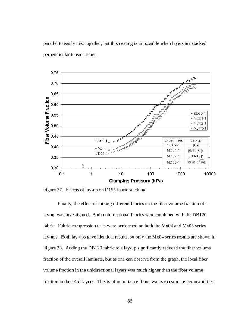
86

parallel to easily nest together, but this nesting is impossible when layers are stacked

perpendicular to each other.

Finally, the effect of mixing different fabrics on the fiber volume fraction of a

lay-up was investigated. Both unidirectional fabrics were combined with the DB120

fabric. Fabric compression tests were performed on both the Mx04 and Mx05 series

lay-ups. Both lay-ups gave identical results, so only the Mx04 series results are shown in

Figure 38. Adding the DB120 fabric to a lay-up significantly reduced the fiber volume

fraction of the overall laminate, but as one can observe from the graph, the local fiber

volume fraction in the unidirectional layers was much higher than the fiber volume

fraction in the ±45° layers. This is of importance if one wants to estimate permeabilities

Figure 37. Effects of lay-up on D155 fabric stacking.

87

of a mixed fabric lay-up since permeability varies greatly with fiber volume fraction. In

addition, it is desirable to know how much relative thickness each layer is taking up in

the laminate.

Permeability

Permeability values were determined for A130, DB120 and D155 fabrics at

several fiber volume fractions. Permeability data are the primary input for any flow

model, so the accuracy of the measurements and calculations is of utmost importance.

Flow results are presented as flow front position versus time in the flat plate mold, see

Figure 20.

Figure 38. Effect of mixed fabrics on fiber volume fraction.

88

A130 Fabric

As stated earlier, A130 fabric is a woven, unidirectional glass fabric. The fiber

tows are woven over a thermoplastic coated glass bead. The thermoplastic bead inhibits

flow through the thickness of a laminate and can create preferential flow between plies.

The glass beads are spaced about every 3 to 4 cm. The perpendicular glass beads create a

channel area that helps in wetting the fabric in the transverse direction.

A contour plot of the resin flow front position over time is shown in Figure 39.

Contours were traced from digitized images of the experiments. The digitized images

were then transformed to a normal unit of measure by knowing distance between pixels.

The mold stiffeners caused the blank areas in the contour plots.

As one can see, the flow fronts were not exactly symmetrical. At the beginning of

the experiment there was some preferential flow on the left-hand side of the mold

(negative x-direction). As the experiment progressed, the flow front shape on the right

hand side of the mold (positive x-direction) passed the flow on the left side. After 30

minutes the right-hand side finished approximately 4 cm further along than the left side.

The transverse direction, however, remained relatively symmetrical. This effect was

commonly observed in unidirectional experiments with the A130 fabrics.

In order to determine the experimental permeabilities, the distance from the inlet

port to the maximum flow front locations in both the transverse and longitudinal

directions were measured and plotted versus time. Since the flow fronts were not

symmetrical, average values were taken in both directions. Figure 40 is a plot of

permeability versus fiber volume fraction.

89

Figure 39. Contour plot for experiment SA08-1. Times are listed in minute_second format on the legend. The lay-up consisted of 8 layers of A130 fabric with a fiber volume fraction of 0.40. Fibers aligned in the x-direction.

Figure 40. A130 unidirectional permeability versus fiber volume fraction.

90

As expected, permeability decreased with increasing fiber volume fraction. The

permeability in the longitudinal direction (Kx) was affected to a greater degree than in the

transverse direction by changing fiber volume fraction.

DB120 Fabric Results

Of the three fabrics tested, the DB120 fabric wet out the most evenly. In addition,

it had a very high through-thickness permeability, due to the fact that it is a stitched

fabric and its fiber bundles are spaced the farthest apart of the three fabrics, Figure 10.

Furthermore, flow experiments with the DB120 fabrics had the smallest region of

unsaturated flow. In most experiments an unsaturated flow region was not noticeable.

One might expect that, since the DB120 contained ±45° plies stitched together,

both the longitudinal and transverse flow directions would be identical, but that is not the

case as can be seen in Figure 41. The exact fiber orientation was checked to see if it was

influencing the flow of resin, however, fibers were orientated 3° towards the transverse

direction. This implies that the increased resin flow in the DB120’s is due to the

presence of the stitching material, which ran parallel to the longitudinal direction.

Comparing Figure 39 and Figure 41, the DB120 fabric shows a much more

symmetrical flow front shape than the A130 fabric. During the course of the experiment,

there was never more than a one cm difference in the two longitudinal flow front

positions. After approximately 2.5 minutes, there was not a significant difference in the

two transverse flow fronts. Similar results were observed with other DB120 fabric tests.

91

Permeabilities of the DB120 fabrics show linear behavior in Figure 42 when

plotted versus fiber volume fraction on a semi-log graph. In addition, both the

longitudinal (Kx) and the transverse (Ky) permeabilities had similar slopes. This is

expected since fabric architecture is similar in both directions.

Figure 41. Contour plot for experiment SB08-1. Times are listed in minute_second format on the legend. The lay-up consisted of 8 layers of DB120 fabric with a fiber volume fraction of 0.31.

92

D155 Fabric

Like the DB120 fabric, the unidirectional D155 fabric consists of stitched fiber

bundles. There were gaps parallel to the direction of the fibers. These gaps create

regions of high permeability. As a result the D155 fabric exhibited highly anisotropic

flow patterns shown in Figure 43. The gaps also raise the through thickness permeability

of the D155 fabric, so preferential flow between fabric layers was not a problem. In

addition, distances between unsaturated flow region were barely noticeable.

Figure 42. Permeability versus fiber volume fraction for DB120 fabric.

93

Both the longitudinal and the transverse flow fronts remained relatively

symmetric. While the shape at the longitudinal ends of the flow front changed slightly on

either side, the maximum flow points from the injection port remained within one cm of

each other throughout the course of the experiment. The maximum flow positions of

transverse flow fronts also remained within one cm of each other throughout the course

of the experiment.

Transverse permeabilities were approximately ten times lower than the

longitudinal permeabilities as shown in Figure 44. Also, as the fiber volume fraction was

increased, the permeability in the transverse direction decreased at a faster rated than the

permeability in the longitudinal direction.

Figure 43. Contour plot for experiment SD06-1. Times are listed in minute_second format on the legend. The lay-up consisted of 6 layers of D155 fabric with a fiber volume fraction of 0.40. Fibers aligned with x-axis.

94

Permeability Discussion

Defining the position of the saturated flow boundary can be a source of error

when calculating permeabilities. An example of this type of flow front is shown in

Figure 45.

Unsaturated flow was a problem primarily in the A130 fabric. In order to

estimate how repeatable these permeability experiments were, a set of three experiments

were performed on an eight-layer lay-up of A130 fabric. Results are summarized below

in Figure 46.

Figure 44. D155 permeability versus fiber volume fraction for a unidirectional lay-up.

95

Figure 45. Unsaturated flow occurring in a unidirectional A130 lay-up.

Figure 46. Permeability variation for three experiments with A130 fabrics.

96

Experiments SA08-1 to SA08-3 used slightly increased fiber volume fraction so a

slight decrease in the longitudinal permeability is expected. However, flow in the

transverse direction did not follow this pattern. The Ky value for the SA08-2 experiment

was slightly higher that the SA08-1 experiment even though it had a one percent higher

fiber volume fraction. In addition, flow in the transverse direction is governed by the

density of cross beads. This tends to vary significantly throughout a roll of fabric. If one

compares the Kx to Ky ratios of the three experiments they differ by about 10% due to the

variability in the Ky measurements.

Permeabilities are summarized for all three fabrics and compared with values

from the NIST Permeability Database18 in Figure 47. Only the NIST permeabilities

Figure 47. Summary of single fabric permeability data.

97

determined through saturated flow experiments were plotted. The unsaturated flow

experiments gave higher permeabilities and may have been influenced by mold

deflections. Trend lines do not include NIST database values.

The longitudinal permeability for the A130 fabric is approximately five times

lower at a given fiber volume fraction than that of the D155 fabric. The decrease in

permeability is due to the smaller channels between fiber bundles in the A130 fabric.

Another factor that restricts flow through the A130 fabric is the glass bead as well as the

thermoplastic used to hold the fiber tows together.

Since fibers are orientated at ±45° relative to the direction of flow, it is not

surprising that the DB120 fabric had the lowest permeability in the longitudinal direction.

However, one can see that below a fiber volume fraction of 0.37 the DB120 fabric has

lower permeabilities than the transverse permeability of the D155 fabric. This may be

due to the lack of compressibility observed in the DB120 fabrics. While both the D155

fabric and the DB120 fabric have the same volume of fibers, the D155’s have their fibers

concentrated into denser bundles. This can leave inter-laminar flow channels at low fiber

volume fractions and increase the transverse permeability of the D155’s.

Another point of interest is how the transverse permeabilities of the A130 and

D155 fabrics varied over the range of fiber volume fractions. At low fiber volume

fractions, the D155 fabric is more permeable than the A130 fabric, but as the fiber

volume fraction increases, the permeability of the D155 fabric decreases at a faster rate

than for the A130 fabric, eventually surpassing it at a fiber volume fraction of 0.40.

Because of the D155 fabric architecture, fiber bundles nest tightly together blocking

98

transverse flow. The A130 fiber bundles, however, are woven over glass beads

orientated in the transverse direction. These weave points create channels in the

transverse direction, even at high fiber volume fractions.

The two unidirectional fabrics, D155 and A130, have large differences between

their longitudinal and transverse permeabilities. D155’s have the largest difference of

approximately an order of magnitude. This is because the D155 fabric has a larger

channel between fiber tows than the other fabrics. The A130 fabric is also different in

that its longitudinal and transverse permeabilities seem to be converging as the fiber

content increases. The A130’s are a woven fabric, so the transverse glass bead creates a

channel, raising the transverse permeability. As expected, the DB120 fabric has a

relatively similar permeability in the two directions since they consist of plies in both the

±45° directions. The DB120’s display slightly anisotropic permeabilities, which is most

likely due to the stitching orientated in the longitudinal direction.

The NIST database contains permeabilities for a large variety of fabrics. NIST

permeability values for the A130 and D155 fabrics are compared with experimental

results from this study to verify that the data are consistent. The NIST database contains

no values for the DB120 fabric, and had no transverse flow properties for the A130

fabric.

Three longitudinal permeability values are given for the A130 fabric in the NIST

Database. They range in fiber volume fraction from 0.365 to 0.446. As one can see in

Figure 47, two of the three NIST Database values agree well with the data from the

present study, 0.446 and 0.371. The other point at 0.365 is approximately twice as high

99

as the results from the present study.

Four longitudinal permeability values are given for the D155 fabric in the NIST

Database. They fell in the fiber volume fraction range of 0.501 to 0.520. If one

extrapolates the curve fit from the present study to this range, the NIST data fall slightly

above the extrapolated trend line, but in the general range predicted.

Finally, the NIST Database gave four transverse permeabilities for the D155

fabric. They fall in the fiber volume fraction range of 0.499 to 0.570. Extrapolation of

the trend predicted from the data from the present study falls slightly above the NIST

data.

Thus, the experimentally determined permeabilities seem to be consistent with

saturated flow experiments measured independently by NIST. The individual fabric

permeability values are now used to predict permeability values for lay-ups containing

various fiber orientations as well as different combinations of fabrics.

Mixed Fabric

The objective of the mixed fabric experiments was to observe the results of lay-

ups containing various fabric orientations as well as lay-ups containing multiple fabric

types. The results were also used to develop a predictive capability for mixed fabrics.

Experimental Results

A total of ten lay-ups are compared in this section. Their permeabilities are

summarized graphically in Figure 48. The naming convention of these lay-ups was

consistent with the rest of the experiments. Lay-ups covered include Mx01 to Mx05.

100

The x designates that either A for A130’s or D for D155’s were the unidirectional

material of the lay-up.

The first lay-up investigated was the Mx01 series lay up, [0/902/0]s. Since the

lay-up contains four layers of fabric in both the 0° and 90° directions, one would expect

the Kx and Ky values to have no significant difference; this is the case with the D155

fabric. The Kx value is 1.98x10-10 m2 while the Ky value is 1.93x10-10 m2. The A130

fabric, however, has a significant difference between its Kx and Ky values. A Kx to Ky

ratio of 2.1:1 is observed. This experiment was repeated with the same result to ensure

that the result was not due to experimental error.

The next lay-up investigated was the Mx02 series, [(90/0)2]s. Once again, this

lay-up contains an equal number of plies in the 0° and 90° directions. Both lay-ups with

Figure 48. Transverse and longitudinal permeabilities for mixed fabric experiments.

101

the A130s and the D155s show almost no significant difference between their Kx and Ky

permeabilities. One interesting point to note: there is a significant drop in the overall

permeability from the MA01 lay-up to the MA02 lay-up. While fiber volume fraction

can play a part in the loss of permeability, experiments MA01-2 and MA02-1 had nearly

identical fiber volume fractions, 0.421 and 0.423, but their permeabilities differ by a

factor of 3.8 for the Kx and 2.0 for the Ky. This effect, however, did not appear between

the MD01 and MD02 lay-ups.

The Mx03 lay-up, [0/90/0/90 ]s, is nearly identical to the Mx02 lay-up if it were

rotated 90°. The only difference being that it does not repeat the 90° layer at the center of

the lay-up. Since it has one less layer than the two previous lay-ups, it has a lower fiber

volume fraction for the same thickness. Thus, it would be expected that the Mx03 lay-up

would have a higher permeability. The data do show this for the A130 lay-up, but not for

the D155 lay-up. Another observation of interest is that the A130 fabric has a rather

large Kx to Ky ratio, while the D155 fabric Kx to Ky ratio is small in comparison. This

would be expected to be the other way around, since the D155 fabric has much higher Kx

to Ky ratios in the unidirectional permeability experiments. One last point to note:

experiment MA03-1 was repeated because it did not contain enough measurements to

give an accurate estimate of the permeabilities; results for the two experiments are

similar.

The next lay-up examined was the Mx04 series, [0/±452/0]s. Either A130 or

D155 fabrics were used for the 0° layers and the DB120 fabric was used for the ±45°

layers. The addition of the DB120 fabric drops the fiber volume fraction of the lay-up

102

significantly, but at the same time has little influence on flow. This can be explained

because the DB120 fabric has relatively low permeabilities even at low fiber volume

fractions. A slight drop in permeability is observed between the MA03 and MA04 lay-

ups even though both have the same relative fiber volume fraction.

Flow front shapes were quite different between the A130 fabric and the D155

fabric under this lay-up. The A130 lay-up has a much lower Kx to Ky ratio than the D155

lay-up. This is expected since the D155 fabric has a much higher permeability in the

longitudinal direction than the A130s

The final mixed fabric lay-up studied was the Mx05 series, [0/±45/90]s. This

lay-up is identical to the Mx04 series except that the 0° plies in the center of the lay-up

are replaced with 90° plies. The addition of the 90° plies would be expected to lower the

longitudinal permeability and raise the transverse permeability relative to the Mx04

lay-up. This is the case in the D155 lay-up, but the A130 lay-up shows a significantly

different result. The MA05 lay-up shows an increase in both longitudinal and transverse

permeabilities when compared with the MA04 lay-up. While the MA05-1 lay-up had a

lower fiber volume fraction than MA04-1, it was not low enough to cause this large of a

change.

Predictive Data used

Permeability data as a function of fiber volume fraction was necessary in order to

predict permeabilities for mixed fabric lay-ups. These data were determined from an

exponential fit to experimentally determined single fabric permeability data, Table 14.

103

The other set of information necessary for predicting permeability in mixed fabric

lay-ups was layer thickness as a function of clamping pressure. These data were taken

from a logarithmic curve fit to experimental fabric compression data, Table 15. Since

clamping pressures were low, only fabric compression data in the range of 3 to 70 kPa

was used to form the correlation. Initial stacking thickness was left out of the curve fit

since it was for fabric under relatively little pressure.

Predictive Results

Graphs comparing the predictions for the Mx01, Mx02 and Mx03 lay-ups to

actual experimental permeability results are shown in Figure 49 and Figure 50. Only the

volume fraction prediction method, Equation 23, is used in these experiments since

results from the fabric stacking experiments were not accurate enough to be able to

Table 14. Correlations for permeability as a function of fiber volume.

Fabric Relation R2 fv

x eK 9.1581085.5 −−⋅= 0.943 A130

fvy eK 63.891013.1 −−⋅= 0.968

fvx eK 2.1391039.6 −−⋅= 0.953

DB120 feK y

7.1491044.6 −−⋅= 0.923 fv

x eK 4.1181030.4 −−⋅= 0.910 D155

fvy eK 3.1781059.3 −−⋅= 0.970

Table 15. Ply thickness versus clamping pressure relationships.

Fabric Relationships R2 A130 ( ) 23 1064.4ln1023.3_ −− ⋅+⋅−= pthickply 0.983

DB120 ( ) 23 1052.5ln1021.4_ −− ⋅+⋅−= pthickply 0.993 D155 ( ) 23 1066.5ln1006.4_ −− ⋅+⋅−= pthickply 0.984

104

determine thickness effects between plies orientated in a unidirectional manner and those

with 0° /90° intersections.

Since all A130 or D155 fabrics were assumed to have the same ply thickness, a

lay-up containing an equal number of plies in the 0° and 90° directions was predicted to

have equal Kx and Ky values as long as it contained only one type of fabric.

This, however, was not the case with the MA01 lay-up. As one can see from

Figure 49 it had a significantly anisotropic flow front. In order to insure that this result

was not caused by an experimental error, the experiment was repeated with the same

result. Permeabilities in both the longitudinal and transverse directions actually are

higher than for a unidirectional lay-up orientated in either direction, Figure 49. This

result is puzzling because a unidirectional lay-up composed of the same material and

Figure 49. Plot of experimental and predicted flow fronts for test MA01-2 at 1800 sec. with an injection pressure of 86.2 kPa.

105

fiber volume fraction should have a higher permeability. The predictions of the

permeability for this lay-up not only fail to capture the general shape of the flow front,

they also under predict flow in the longitudinal direction by 43% and under predict flow

in the transverse direction by 17% after 1800 s.

Flow fronts were next plotted for the MD01 lay-up in Figure 50. Once again

relative thickness estimates used the information in Table 14 and Equation 23 to estimate

permeability for the relative thickness method.

The MD01 lay-up had an isotropic flow front as predicted. Once again flow was

under predicted. However flow in the D155 fabric stayed within the range predicted by

Figure 50. Plot of experimental and predicted flow front positions for test MD01-1 at 500 sec. with an injection pressure of 89.7 kPa.

106

the longitudinal and transverse permeabilities for a unidirectional lay-up at the same fiber

volume fraction. While permeabilities were off by nearly 30%, flow front position in the

transverse and longitudinal was under predicted by only 15%. A probable cause of the

under prediction in flow is that flow permeates the fabric faster in the 0° layers, thus

wetting out the 90° plies through the thickness of the fabric.

Both the MA02 and the MD02 lay-ups had isotropic flow fronts. The

permeability of the MA02 lay-up dropped by a factor of 3.8 in the longitudinal direction

compared to the MA01 lay-up. This lay-up was much closer to the predicted

permeability, with permeability over predicted by 15%.

The experimental permeabilities of the MD02 lay-up dropped compared to MD01

even though they were predicted to increase, due to a decreased fiber volume fraction,

Figure 51 and Figure 52. This decrease in permeability is most likely due to

experimental variation, as the permeabilities of the MD02 experiment are only under

predicted by 11%.

Since the Mx03 series of lay-ups had four layers in the 0° direction and only three

in the 90° direction it was predicted that the permeability of these lay-ups would be

higher in the longitudinal direction. Although this was the case, the magnitude of the

difference between the longitudinal and the transverse permeabilities was not accurately

predicted for all cases. The MA03 lay-up was under predicted by a factor of 2.5 in the

longitudinal direction but only under predicted by 22% in the transverse direction. It is

worth noting that the trend of significantly under predicting longitudinal permeabilities

was also observed in the MA01 lay-ups. This, however, is not as readily dismissed in the

107

MA03 lay-up since this lay-up does not contain any adjacent layers with the same

orientation.

The predicted shape of the MD03 lay-up flow front was much closer to

experimental observations than was the case with the MA03 lay-up. A Kx to Ky ratio of

1.28 was predicted, while a Kx to Ky ratio of 1.17 was observed. Longitudinal

permeability values were over predicted by 55% while the transverse permeabilities were

over predicted by 69%.

Figure 51. Summary of longitudinal permeability estimates versus experimentally determined permeabilities for the Mx01, Mx02 and Mx03 series lay-ups.

108

Graphs comparing both the relative thickness and the clamping pressure

predictive methods of the Mx04 and Mx05 lay-ups to experimental results are shown in

Figure 53 and Figure 54.

As mentioned earlier, the relative thickness method used the fiber volume fraction

of the entire lay-up to predict permeabilities for each fabric layer. Then, the number of

plies of a given fabric and its relative thickness are used to estimate its overall fraction of

the lay-up.

The clamping pressure method, on the other hand, used a clamping pressure to

determine the thickness and fiber volume fraction of each individual fabric present in the

Figure 52. Summary of transverse permeability predictions versus experimentally determined permeabilities for the Mx01, Mx02 and Mx03 series lay-ups.

109

lay-up. Table 16 compares input data for the Mx04 and Mx05 lay-ups.

The relative thickness method predicts the same fiber volume fraction for both the

unidirectional layer and the DB120 layer, while the clamping pressure method predicts

the DB120 fabric will have a lower local fiber volume fraction than the unidirectional

fabric. Also, the clamping pressure method predicts that the DB120 fabric will take up a

larger fraction of the composite than does the relative thickness method.

The clamping pressure method consistently predicts lower permeabilities in the

longitudinal direction than the relative thickness method, see Figure 53. This is a direct

result of the thicker DB120 layers predicted by this method and the higher local fiber

volume fractions in the unidirectional material. As was demonstrated earlier, the DB120

fabric has a much lower permeability than the unidirectional material in the longitudinal

direction even at much lower fiber volume fractions, see Figure 47. This effect is

magnified in the MD04 and MD05 series since the permeability of the D155s is much

higher in the longitudinal direction than for the A130s.

In general, predictions from the relative thickness method were closer to the

experimentally observed Kx results than the predictions from the more complex clamping

Table 16. Predicted lay-up composition and permeabilities for Mx04 and Mx05 lay-ups.

Lay-Up Method % DB120 by volume

vf for 0° layer

vf for DB120’s Kx (m2) Ky (m2)

Rel. Thk. 44.6 0.340 0.340 1.11x10-10 3.80x10-11 MA04 clamp 53.9 0.445 0.306 8.22x10-11 4.91x10-11 Rel. Thk. 44.6 0.394 0.394 3.00x10-10 3.11x10-10 MD04 clamp 49.0 0.462 0.324 1.56x10-10 3.28x10-11 Rel. Thk. 40.2 0.366 0.366 1.14x10-10 1.03x10-10 MA05 clamp 54.1 0.415 0.284 1.06x10-10 7.88x10-11 Rel. Thk. 40.2 0.367 0.367 2.33x10-10 2.25x10-10 MD05 clamp 49.1 0.432 0.301 1.43x10-10 1.22x10-10

110

pressure method. The clamping pressure method was able to predict a large relative

increase between the MA04 and MA05 lay-up while the relative thickness method was

not. In addition, the clamping pressure method consistently under predicts permeabilities

in the longitudinal direction while the relative thickness method underpredicts for the

A130 lay-ups and overpredictes the D155 lay-ups.

It is shown in Figure 54 that the clamping pressure method estimates the effect of

the addition of 90° plies to the lay-up more accurately than does the relative thickness

method. The relative thickness method greatly exaggerates this effect in both the A130

and D155 lay-ups, while the clamping pressure method follows the experimental data

more closely. Once again, the clamping pressure method consistently under estimates the

Figure 53. Predicted versus experimental Kx values for the Mx04 and Mx05 lay-ups.

111

permeabilities in the y direction while the relative thickness method under predicts for all

but the MD05 experiment. Also, the clamping pressure method predicts permeabilities

closer to the experimentally observed Ky values for all the experiments except MA04.

Table 17 indicates that the clamping pressure method flow front predictions were

closer to experimental than those predicted by the relative thickness method for all

experiments. Both methods failed to capture the flow front change between the MA04

and MA05 experiments. Because the clamping pressure method under predicts flow

fronts in the longitudinal direction, its flow front ratios, while close, were consistently

lower than the experimental ratios. The relative thickness method over predicts the flow

contribution in the longitudinal direction for the Mx04 experiments, and under predicts

Figure 54. Predicted versus experimental Ky values for the Mx04 and Mx05 lay-ups.

112

its contribution in the Mx05 experiments. This trend was most obvious with the D155

lay-ups. Overall, the clamping pressure method did a better job of capturing flow effects

in mixed fabric lay-ups.

Summary

Although both the A130s and D155s are unidirectional fabrics, they did not

always follow the same trends. One would expect the Mx01 series lay-up to have equal

permeabilities in both principal directions. However, the flow front for the MA01 lay-up

with A130 fabric was highly orientated in the longitudinal direction. It was not

uncommon for lay-ups containing two consecutive layers of 90° plies to have much

higher permeabilities in the longitudinal direction than expected, examples are MA01 and

MA05.

Two predictive methods were used to estimate the permeability of a mixed fabric

lay-up. The first method was the relative thickness method. In order to determine the

composition of a lay-up containing two separate fabrics, the relative thickness data for

each fabric was used to estimate their fraction of the lay-up. Then, the fiber volume

fraction of the entire lay-up used for each ply, whether they were different fabrics or not.

The clamping pressure method used clamping pressure data to estimate the thickness

Table 17. Comparison of predicted to experimental flow front shapes.

Experiment Experimental Kx/Ky

Clamping Pressure Kx/Ky

Relative Thickness Kx/Ky

MA04-1 1.72 1.67 2.93 MA05-1 2.03 1.34 1.11 MD04-1 5.85 4.74 9.67 MD05-1 1.32 1.17 1.04

113

contribution of each fabric as well as its fiber volume fraction. That way each fabric may

be at a different fiber volume fraction. Once again, the layer permeabilities are combined

into a single permeability using Equation 23.

The methods were able to predict the general trends for most lay-ups. Both

methods were not able to accurately predict flow in lay-ups containing A130’s orientated

at 90°. Generally, flow was greatly under predicted in these lay-ups. In addition,

permeabilities predicted by the clamping pressure method represented what was observed

experimentally, both in shape and magnitude, and were closer than the relative thickness

method.

T-Section

The foregoing findings were next applied to the T-section geometry, Figure 21

and 55, which has three-dimensional flow characteristics. This mold contained two

intersecting flow planes as well as three regions of differing thickness. Experiments were

performed with both central and end injection points: TA01 and TD01 were central

injections and TA02 was an end injection. The lay-ups orientation and fiber contents for

each section are given in Table 9.

TA01

A plot showing flow contours for the TA01 experiment is given in Figure 56.

Contours are separated into the web and skin planes because information would have

been lost in a three-dimensional plot. The skin surface of the mold was aligned

perpendicular to the ground, and the web plane was parallel to the ground. Injection took

114

place from two symmetrically spaced injection ports. The ports were located halfway

along the length and injected through the flange area of the mold, Figure 56. Also, the

lay-up was selected to keep similar fiber volume fractions in all three sections of the

mold: skin, flange and web.

At the injection ports in the flange region, the part was approximately 1.30 cm

thick, while farther on the skin stepped down to 0.284 cm thick. Resin first penetrates the

skin at this step area at the 46-second mark⎯approximately 4.6 cm from the skin-web

intersection. As one can see, it took a considerable amount of time before the resin

penetrated through the fabric comprising the flange and skin. In addition it took a

considerable amount of time, 6 minutes, before the flange was fully wet-out near the

injection ports. Resin did not penetrate the skin surface symmetrically. The resin

penetrated the bottom half of the skin nearly 2 minutes before it started penetrating

through the top half of the skin. Wet-out in the skin surface of the mold was achieved by

the bottom half of the mold filling. At this time, the preferential flow along the edges of

the mold was the primary source of flow. This eventually created an air pocket on the top

half of the skin section. Injection was halted after fifteen minutes and this region failed

to completely wet out.

Flow proceeded at a much more rapid rate in the web section. Even though the

photographs at the web did not turn out, resin had penetrated beyond the region blocked

by the mold at the time the first images were recorded, 1 min 24 s. Since resin was able

to stay in the plane of the fibers in the web section, the majority of the resin went there

instead of flowing through the plane of the fabric into the skin/flange section. Once

115

again, preferential flow occurred along of the boundary of the mold, trapping an air

pocket in the web section.

Around the three-minute mark, resin had penetrated the entire length of the web

section. A factor that greatly increased the permeability in the x-direction of the mold

was a region of low fiber volume fraction caused by the fabric architecture at the skin-

web interface as shown in Figure 55. A cross-section of an actual composite part

showing this void area can be see in Figure 13.

Unfortunately, it was difficult to eliminate preferential flow (race tracking)

problems in the thick flanged T-mold. Even if one was careful cutting and placing fabric,

the shape of the mold along the z borders of the skin plane make it impossible to prevent

preferential flow in that direction. Preferential flow also occurred in the region where the

flange stepped into the skin, as a result of the void region created by the lay-up geometry.

In addition, the low out-of-plane permeability of the A130’s created preferential flow

Figure 55. Source of high permeability in T-sections.

116

between layers. Flow in the flange region progressed through the bottom layers first

before it penetrated the entire thickness. An example of flow patterns caused by

preferential flow between layers can be seen in Figure 56.

TD01

A plot containing flow contours for TD01 is shown in Figure 57. The mold and

setup procedures were identical to those used for the TA01 experiment. In addition to

Figure 56. Flow front positions for TA01. Injection was from two central injection ports (shown as black dots) at a pressure of 82.7 kPa.

117

using D155s instead of A130s, the lay-up of the TD01 differed from the two A130

T-section lay-ups. The A130 lay-ups were chosen to give similar fiber volume fractions

in the skin, flange and web sections of the mold. This experiment, however, had

significantly different permeabilities in each section.

Unlike the A130 lay-up, the D155 fabric allowed the resin to penetrate the skin

surface easily. In addition, flow patterns from both injection ports were relatively

symmetrical, the flow front from the upper port advancing slightly faster. Flow advanced

faster on the left side of the mold. It nearly completed filling around the 11 minute mark,

while a substantial air pocket still existed along the right side of the mold after 15

minutes. It can be seen from the flow fronts that the permeability of the skin region on

the skin surface was lower than the permeability in the flange region. This was a result of

the skin region having a much higher fiber volume fraction than the flange region.

Flow was not visible in the T-section until three minutes and 45 seconds into

injection. Resin penetrated the y direction slowly since it was flowing normal to the

D155 fibers . Flow progressed across the right side of the web faster than it moved

through the left side, opposite of the skin surface. Flow had completely filled the right

hand side of the web at the 12 minute 14 second mark.

Race tracking occurred in the both the skin and the web sections of the mold, but

race tracking was not nearly as pronounced as with the A130 fabric. In addition, the high

permeability through the plane of the D155’s allowed the resin to evenly penetrate the

flange section of the mold, unlike with the A130’s. This gave flow fronts with smooth

surfaces and no resin pockets ahead of the main flow front. Flow into the web section

118

was hindered by the low permeability normal to the D155 fibers. This is evident by the

flat flow fronts in that section, and is contrasted by the A130 lay-up.

TA02

A plot containing flow contours for TA02 is shown in Figure 58. The mold and

setup procedures were identical to those used for the TA01 experiments. The only

difference being that injection took place at the end of the mold instead of at the center.

Figure 57. Flow front positions TD01. Injection was from two central injection ports (shown as black dots) at a pressure of 82.7 kPa.

119

Although the injection ports were located at the flange, resin quickly spread

across the skin surface in the z direction as well as through the thickness of the flange due

to race tracking. As one can see, flow along the skin surface started out symmetrical.

Then, after three minutes, edge effects as well as the seemingly lower permeability of the

flange region gradually influenced flow. Resin reached the far end of the skin section

around 11 minutes, but as in the previous experiment, this was simply a result of

preferential flow along the edges of the mold. Flow then trapped an air pocket in the skin

section around the 16-minute mark. The skin surface finally finished wetting out 25

minutes 17 seconds into the experiment.

The main mechanism of flow in the web section was flow along the web/skin

intersection. This problem was exacerbated by the fact that skin and web mold faces

were not exactly aligned, so the actual thickness of the part was 0.5 mm greater in this

region. At the time the resin reached the end of the mold in the web section, it had

traveled nearly 55 cm, while at the same time resin had only advanced 25 cm in the skin

section. After the resin reached the end the mold, it traveled to the skin layer as well as

down into the web section. Judging by the flow fronts, preferential flow was once again

a factor along both x boundaries as well as the y boundary of the web. Air was also

trapped in the web section, and the web finished wetting out after 29 minutes.

In addition to race tracking complications, inter-laminar preferential flow was

present in the skin section. Although it was not as pronounced as in the TA01

experiment, pockets of resin were observed ahead of the flow front between times of 7 to

10 minutes.

120

Steel Root Insert Mold

Since the steel insert mold was opaque, a partial injection was required to get an

idea of the filling patterns inside the mold. The mold was filled for 160 seconds and then

Figure 58. Flow front positions for TA02. Injection was from two injection ports located at the end of the mold. Injection pressure was at 82.7 kPa.

121

the resin was allowed to cure. After the part cured it was removed and the flow fronts

were analyzed. As one can see from Figure 59, filling patterns differed on the skin and

inner surface sides of the mold. This was a result of the injection port being located

under the steel insert on the skin side of the mold.

Flow first progressed across the skin side of the mold. The flow seemed slightly

biased along the length of the mold. As one can see there was a bit of race tracking on

the top half of the skin. Additional fabric was placed in this region to build up the fiber

volume fraction, but it may have been displaced when the mold was put together.

Flow may have reached the inner-surface face of the mold by either of two

mechanisms. Either flow progressed through the lay-up and around the steel insert, or it

reached the boundary of the mold on the skin surface and penetrated to the surface.

Judging by the lengths of the two flow fronts on the inner-surface mold, it is expected

that the flow reached the boundary before flow had completely penetrated into the inner

surface side of the mold. This, however, was due to race tracking, and judging by the

results it appears that normally flow would penetrate the inner-surface face of the

laminate before flow reached the boundary on the skin face.

During the complete filling of the mold, flow reached the vent port on the insert

side of the mold approximately 238 seconds after injection. The mold was completely

filled at 741 seconds.

122

Figure 59. Filling pattern of insert mold with an injection pressure of 96.5 kPa.

123

CHAPTER 5

NUMERICAL RESULTS AND CORRELATION WITH EXPERIMENTS

LIMS basics

Liquid Injection Modeling Simulation 4.0 (LIMS) is a finite element based

program that is specialized for modeling fluid flow in RTM molds. LIMS only accepts a

mesh composed of 4 node quadrilateral elements. LIMS uses Darcy’s law combined with

a boundary element method to advance flow, and conservation of mass issues are

addressed by assigning a fill factor to the nodes.

In order to analyze flow for a given mold one must follow these steps: create and

mesh the model; define permeabilities throughout the mold on an element by element

basis; set the port type, initial value and nodal location; and record or display the desired

information.

Model Creation

One feature that sets LIMS apart from other RTM modeling software packages is

its ability to read models created from third party software. LIMS will read finite

element models created in PATRAN and exported as neutral files. A limitation of LIMS

is that it requires linear quadrilateral elements. These shell elements allow one to model

three-dimensional shapes, but do not account for flow through the thickness of a

laminate. LIMS requires that all duplicate nodes at intersections must be removed, and

124

the model must be renumbered so the list of nodes and elements is continuous. In

addition, one must keep track of element normals to insure proper translation of the

model.

One parameter of interest is the sensitivity of the results to the density of the

mesh. To determine this, test runs were done at several mesh densities. A common way

to do this is to vary the mesh size and solve the model. As the mesh size is decreased, the

solutions should converge. The only parameters varied in this set of tests were the

element size and the injection pressure (flow rate). A matrix of numerical sensitivity

tests performed is shown in Table 18. Tests were done simulating a center injection on

the flat plate mold. Flow distances were then recorded along the x and y axes with the

injection port being located at the origin. In addition, two pressures were used to see if

the accuracy of the model depends on the velocity of the flow front.

Although boundary conditions may not be specified into LIMS, it is possible to

exploit symmetry since flow along a plane of symmetry and flow along a solid boundary

are treated the same. This was verified by comparing two models with the same element

Table 18. Matrix of mesh sensitivity runs on a 510 mm by 810 mm plate model with quarter symmetry and the injection port located at the origin.

Trial element length (mm)

Injection Press. (kPa) x direction times (s) y direction times (s)

1 50.8 89.7 150, 450, 900 150, 450 2 25.4 89.7 150, 450, 900 150, 450 3 12.7 89.7 150, 450, 900 150, 450 4 6.35 89.7 150, 450, 900 150, 450 5 50.8 160 150, 450 150, 450 6 25.4 160 150, 450 150, 450 7 12.7 160 150, 450 150, 450 8 6.35 160 150, 450 150, 450

125

edge length, one with quarter symmetry and one without. Therefore, in the mesh

sensitivity runs, the model employed quarter symmetry on the flat plate mold in order to

minimize the number of elements required and solution time.

As one can see from the results, Table 19, at lower mesh densities flow seems to

be faster. If one had a poorly meshed model errors could become quite large. In

addition, as time progressed the difference between the dense and fine mesh increased

slightly. As one can see from trials 1 to 4, flow values in the y direction were much

closer at the different mesh densities than in the x direction. It was of interest to see if the

rate of flow made a difference in the accuracy of the results, so the pressure of the

experiment was increased. As one can see from trials 5 to 8 there was less of a difference

between the fine and coarse meshes as the flow rate increased.

Judging from the convergence runs, the error of a model tended to be on the order

of the element size. Early in the experiment, 150 seconds, the error was approximately

half the size of an element, and towards the end, at 900 seconds, it was slightly larger

than the size of an element.

Table 19. Mesh sensitivity flow results.

trial x flow distance (cm) y flow distance (cm) @ 150 s @450 s @900 s @150 s @450 s 1 16.33 25.98 35.06 10.85 17.39 2 14.66 23.75 32.38 9.97 16.28 3 13.5 22.11 30.24 9.28 15.32 4 12.59 20.71 28.41 8.73 14.42 5 20.89 33.27 na 13.84 24.2 6 18.87 30.78 na 12.91 21.19 7 17.51 28.71 na 12.07 19.92 8 16.37 26.97 na 11.37 18.78

126

LIMS input parameters

Once meshed, a LIMS model must be formatted. In addition to creating a list of

node locations and element connectivities, LIMS gathers the model parameters given in

Table 20 from user input.

K11 is the permeability of the fabric in the longitudinal direction, K22 the

permeability in the transverse direction and K12 the flow coupling term in the

permeability tensor. In addition, the fiber volume fraction (vf) as well as resin viscosity

were needed. The IAX term defines the longitudinal direction of an element in the global

x-y-z coordinates of the mold. The designation 1 would mean the longitudinal direction

is the x direction, a 2 would mean it was in the y direction and a 3 would make the

longitudinal direction the z direction. If one selects a value for IAX that is perpendicular

to the element, an error results. Next, LIMS requires an element thickness; element

thickness does not seem to have an effect on the flow, as shown by trials done with

models having two different element thicknesses. Finally, injection and vent port

information may be added at this time. LIMS supports three types of injection ports:

constant pressure, constant flow rate and mixed gates. Mixed gates generally are a

constant flow rate gate that can not exceed a maximum pressure, so once that maximum

pressure is reached it becomes a constant pressure gate.

Table 20. LIMS input parameters

K11 vf K22 resin viscosity K12 element thickness IAX port information

127

Recording information

Another feature of LIMS is its flexibility in recording data. It contains a set of

commands called lBasic that allow the user to manipulate the injection and record results.

LBasic allows the user to control ports during the course of an injection as well as record

information at any node in the model. Parameters that may be monitored include: time,

fill factor, pressure, number of empty or filled nodes during last time step and fill time for

a particular node. If one wishes to learn more about the features available they should

refer to the LIMS users manual, Reference 36. Once the model has been solved LIMS

may also format the results for plotting. Available FEA post processing formats include

Tecplot and PATRAN.

Flat Plate models

The first step in modeling parts was to verify the accuracy of the model on a

simple flat plate structure. The model was used to determine the experimental errors

associated with calculating permeabilities. Then A130 and D155 lay-ups were

investigated to see if LIMS could accurately predict flow front shapes of the more

extreme experimental results. Next, permeability predictions for lay-ups combining

unidirectional fabric with the DB120 fabric were examined. Finally, lay-ups that were

not well predicted by the permeability estimation schemes were analyzed.

Two different models were used to represent the flat plate. The first had an

element edge length of 12.7 mm and modeled the entire plate. The other model used

quarter symmetry and an element edge length of 6.35 mm. All models represented the

mold with an injection port at the center. In addition, the injection was placed at the

128

origin for all flat plate runs.

Experimental Error

There were several sources of error when determining and locating the flow front

positions. There was a ±3.45 kPa pressure difference, generally ±3.8%, during the

experiment. Errors measuring fiber volume fraction and part thickness contributed to

incorrect input into the model. Also, the process of digitizing the flow fronts added some

error to flow front measurements.

Of the above mentioned sources of error, pressure fluctuation during the course of

an experiment was the most significant. It could result in a maximum flow front position

error of one cm after 1200 seconds of injection time. A similar magnitude of error could

be realized if the fiber volume fraction was off by more than 0.03; typical experimental

errors are in the ±0.01 range. The inaccuracy associated with measuring part thickness

and errors from digitizing flow fronts only contributed errors on the order of 1mm or less.

A130 08 Lay-up (SA08-1)

All the single fabric experiments should have been modeled exactly since the

permeability is reduced from the experiment it is modeling. This particular lay-up,

however, had an asymmetrical flow front. Most lay-ups had higher permeability in the

longitudinal direction than in the transverse direction, but this lay-up had slightly

different permeabilities in all four directions. This phenomenon happened in a few of the

experiments, but was the most severe with this lay-up.

As one can see from the diagram in Figure 60, experimental flow in the

129

longitudinal direction initially started out faster on the left-hand side of the mold. At 150

seconds flow on the right side of the mold exceeded flow on the left and that trend

continued for the remainder of the experiment. By 1620 seconds there was

approximately a 4 cm difference in flow between the two longitudinal flow fronts. LIMS

seemed to slightly under predict flow in the longitudinal direction throughout the course

of the experiment and the difference was at a maximum of 8% at 1620 seconds.

Flow in the transverse direction was much more symmetric than in the

longitudinal direction, and the model predicted flow results much closer than those in the

longitudinal direction. Once again, however, the model under predicted flow, with flow

being under predicted by a maximum of 11% at 1620 seconds.

The model predicted a smooth, rounded flow front. As one can see, the flow front

Figure 60. Experimental versus predicted flow front positions for SA08-1, single fabric A130. Kx=9.90x10-11 Ky=3.47x10-11, vf=0.400, µ=0.195 kg/m⋅s and P=89.7 kPa.

130

shapes predicted by the model were quite close to those observed experimentally. The

left-hand side of the plate was modeled within experimental error. However, flow on the

right-hand side of the mold came to a point and was approximately 4 cm ahead of the

model prediction at the end of the experiment (1620 s). The shape of the model along the

transverse flow front closely matched the experimental shapes on both sides. Since the

model assumed symmetry, differences from symmetrical flow fronts could not be

predicted, nor could they have been if the whole plate were modeled.

D155 06 Lay-up (SD06-1)

The SD06-1 experiment was also a single fabric lay-up used to determine

permeability. Because of the large difference between the permeabilities of the

longitudinal and transverse directions, it was of interest to see if the model would

accurately predict the shapes of the flow fronts as well as the curvature along the

longitudinal axis.

As shown in Figure 61, flow distances along the longitudinal axis were predicted

relatively well using the higher mesh density model. The maximum error in predicting

the flow distance was roughly 1 cm after 560 seconds of injection time. The lower mesh

density model, element edge length of 12.7 mm, was not as accurate. In the worst case it

over predicted flow by nearly 4 cm along the longitudinal axis. Thus the error is greater

using lower mesh densities when the flow fronts have a tighter radius.

Experimental flow in the transverse direction was shifted towards the bottom half

of the mold; however, flow was well predicted by both models. Flow distances were

predicted to within 1 cm.

131

Flow front shapes predicted by the model were close to those observed

experimentally. Experimental flow fronts tended to have a smaller radius for the

longitudinal direction. This caused the model to slightly over predict flow in the

transverse direction near the tip of the longitudinal flow front.

A130-DB120 [0/±452/0]s Lay-up

The objective of modeling the MA04-1 lay-up was to show how the two

permeability estimation schemes, relative thickness and clamping pressure, compared

with experimental results. Since it has already been demonstrated that experimentally

determined permeabilities accurately represent flow even in the extreme cases,

experimentally determined permeabilities were used to give the flow front locations of

the experiment instead of actual experimental data in Figure 62. While experiments with

Figure 61. Experimental versus predicted results for SD06-1, single fabric D155. Kx=6.16x10-10 Ky=4.80x10-11, vf=0.398, µ=0.195 kg/m⋅s and P=89.7 kPa.

132

the D155 and DB120 fabrics were better predicted than those with the A130 and DB120

fabrics, the latter results are given in Figure 62 because they better represented the MSU

composite version of the AOC 15/50 blade.

Neither of the models predicted flow accurately. The relative thickness method

was the least accurate of the two, under predicting flow by 3 cm after 1800 seconds in the

longitudinal direction and under predicting flow by nearly 7 cm in the transverse

direction after 1800 seconds. In addition, it failed to calculate the proper shape of the

flow front. While the clamping pressure method under predicted flow in the longitudinal

and transverse directions by approximately 5 cm, it captured the proper shape of the flow

front. The greater accuracy of the clamping pressure method appears to validate one of

its main features: fiber volume fraction varies in plies with different fabrics.

Figure 62. Flow contours comparing the experimentally determined permeability with two predictive methods. Flow front times are at 85 and 1800s from an injection port located at the origin. Quarter symmetry was assumed.

133

A130 [0/90/0/90 ]s Lay-up

The MA03-2 lay-up was selected because it was a worst case scenario. Of all the

mixed fabric permeability cases, the MA03 lay-up resulted in one of the least accurate

predictions using unidirectional ply permeability data.

As one can see from Figure 63, flow is relatively well predicted in the transverse

direction. However, the flow front location in the longitudinal direction is nearly 580 s

behind after 900 s of injection. Because of this, the predicted permeability fails to

capture the correct shape of the flow front. While these results are not encouraging, they

are only a factor of 2 off at a worst case scenario. However, if one wants to accurately

model flow front shapes and injection times, it would be best to determine the exact

permeability from an experiment instead of trying to produce permeabilities from

unidirectional fabric permeabilities.

Figure 63. Flow contours comparing the experimentally determined permeability with the relative thickness predictive method for the MA03-2 lay-up (0/90/0/90 )s. Flow front times were at 54 s, 320s and 900 s from an injection port located at the origin. Quarter symmetry was assumed.

134

T-section Results

T-intersections are a major feature of a turbine blade geometry, and also represent

a basic three-dimensional geometry case. T-sections were modeled with injection ports

located at both the center of the mold and at the ends using mixed lay-ups of either A130

or D155 fabric with the DB120 fabric.

Thick flanged T model

The thick flanged T was modeled with half symmetry along the web plane.

Quarter symmetry was not chosen because injections were also performed from the ends

of the mold and it was desired that the same model be used for both the end and central

injections.

In order to take into account the different geometries and lay-ups present in the

thick flange T-mold, it was divided into three regions with different permeability

properties: skin, flange and web. The meshed version of this model is shown in Figure

64. The model contained 2376 elements, with a maximum edge length of 5 mm.

Elements 1-1296 made up the web section, elements 2397 to 1836 made up the flange

region, and elements 1837 to 2376 made up the skin region. Since the permeabilities of

the three regions varied from experiment to experiment they will be detailed in the

relevant sections.

135

A130 Center Injected T-mold (TA01)

The LIMS input parameters used for modeling the TA01 experiment are shown in

Table 21. All permeabilities were calculated by using the clamping pressure method.

The lay-up was chosen to give a consistent fiber volume fraction throughout the part.

As one can see from Figure 65 it is difficult to determine how accurate the model

was in predicting flow patterns. There was a considerable amount of interlaminar flow

Figure 64. Meshed T-mold showing the three different lay-up regions.

Table 21. Fabric related LIMS input properties for thick flanged T model TA01. Injection took place at 82.7 kPa from a central injection port and with a resin viscosity of 0.195 kg/m⋅s.

Skin Flange Web Kx (m2) 1.41⋅10-10 1.63⋅10-10 9.91⋅10-11 Ky (m2) 7.10⋅10-11 9.29⋅10-11 6.10⋅10-11

vf 0.346 0.316 0.342 Thickness (cm) 0.283 1.283 0.532

elements 1837 - 2376 1297 - 1836 1 - 1296

136

that the LIMS model cannot predict because it uses 2-D shell elements which do not

account for flow through the thickness of the element nor does allow for an element to be

composed of several layers of material. In addition to the interlaminar flow, there was a

considerable amount of racetracking present along the borders of the mold in the

experiment. This is most visible in the web section where flow quickly progressed along

the mold border in the y direction. The model gives an accurate prediction of flow front

shape in the web section of the part. This indicates that the Kx and Ky permeabilities in

that region were in the same relative magnitude to each other as were the experimental

values. However, the model did not predict flow to be at the first experimental contour

level, 155 seconds, until 300 seconds had passed. Although the filling patterns in the rest

of the mold were inconclusive, the filling time predicted by the model, 1032 seconds, is

close to the experimental filling time of 1200 seconds.

D155 Center Injected T-mold (TD01)

The LIMS input parameters used for modeling the TD01 experiment are shown in

Table 22. Once again injection took place at centrally placed injection ports. This lay-up

was selected to contrast the filling patterns of the A130 fabric since the through-thickness

permeability of the D155’s is considerably higher than that of the A130’s. Permeabilities

in the three sections differed a bit more than for the A130 lay-ups. All permeabilities

were calculated by using the clamping pressure method.

137

Figure 65. Predicted versus experimental results for case TA01.

Table 22. Fabric related LIMS input properties for thick flanged T model TD01. Injection took place at 82.7 kPa from a central injection port and with a resin viscosity of 0.195 kg/m⋅s.

Skin Flange Web Kx (m2) 2.17⋅10-10 7.13⋅10-10 7.25⋅10-10 Ky (m2) 8.64⋅10-11 1.90⋅10-10 1.94⋅10-10

vf 0.333 0.273 0.271 Thickness (cm) 0.294 1.281 0.515

elements 1837-2376 1297-1836 1-1296

138

The predicted filling times shown in Figure 66 do not match well to the

experimental flow fronts. The model predicts filling times to be significantly shorter than

experimental values. The flat plate cases gave predicted results which showed that

permeabilities were consistently under predicted, giving longer than actual filling times.

The cause of this was that the experiment had problems with the mold sealing. This was

most likely the cause of the discrepancy between the predicted filling time of 337 seconds

and the actual filling time in excess of 900 seconds for the T-section case TD01.

Although the filling times did not match, the flow front shapes seem to be

reasonably close to those predicted by the model. Both the model and the experiment

show a higher transverse permeability in the flange region. In addition, the relative

differences between the transverse permeabilities in the flange and skin sections seems to

be predicted relatively well. Also, flow fronts predicted in the web region have nearly

the same shape as those observed experimentally. This leads one to believe that the

transverse and longitudinal permeabilities in the web have the correct relative

magnitudes. There was race tracking observed in the mold, but it was significantly less

than the amount present when using the A130 fabric in the same mold.

139

A130 End Injected T-mold (TA02)

The LIMS input parameters used for modeling the TA02 case are shown in Table

23. All permeabilities were calculated by using the clamping pressure method. Injection

was from the end of the mold instead of in the center as in the previous two cases. Due to

the shape of the mold, a large resin rich region filled at the start of the injection along the

skin surface. To model this effect more accurately, injection ports were located along the

length of the skin in the z direction instead of at a single node.

Figure 66. Predicted versus experimental results for case TD01.

140

Once again flow front shapes were not well predicted. The model predicted the

flange region to be slightly less permeable than the rest of the skin section. Judging from

the experimental results, the model seemed to under predict the magnitude of the

difference. However, race tracking along the skin boundaries in the x direction also

contributed to the higher permeabilities, so it is difficult to determine whether the model

predicted the correct ratio of permeabilities between the flange and skin regions.

Experimentally, flow in the web was governed by transverse flow into the web from the

skin/flange intersection, while the model predicted flow to originate from a single point at

the skin/flange intersection. As one can see, the experimental flow front reached the end

of the mold, along the skin/flange intersection, after 420 seconds, but the model predicted

flow to be slightly less then halfway across the mold at this time. The two flow fronts are

considerably different. Despite the inability to predict the preferential flow in the

experiment, the filling times predicted by the model are close to experimental values.

The model predicted filling to be completed at the 1886 s mark, compared to the

experimental value of 1740 seconds.

Table 23. Fabric related LIMS input properties for thick flanged T model TA02. Injection took place at 82.7 kPa from an end of the skin. A resin viscosity of 0.195 kg/m⋅s was used.

Skin Flange Web Kx (m2) 1.72⋅10-10 1.78⋅10-10 9.75⋅10-11 Ky (m2) 8.31⋅10-11 1.01⋅10-10 6.00⋅10-11

vf 0.331 0.310 0.343 Thickness (cm) 0.295 1.31 0.530

elements 1837-2376 1297-1836 1-1296

141

Steel Insert Results

The steel insert mold provides several interesting features. First, it has a very

complex lay-up containing ply-drops, several fabrics and even fabric rolled into dart

shapes. All these effects will be taken into account with a smeared permeability. In

addition, the mold is relatively thick, and experimentally it was shown that flow through

the thickness was significant around the steel insert. The objective of attempting to

model this part was to see how much error results from permeability estimates, as well as

the inability of the modeling program to deal with fully three dimensional flow patterns.

Figure 67. Experimental versus predicted results for TA02.

142

Insert Model

Due to the location of the injection port half symmetry was used along the x axis

of the part, Figure 68. The insert mold was modeled with two surfaces. The first was the

flat, skin surface of the mold. The skin surface covered the entire mold. The other was

the curved, inner-surface side that was only present in the insert region. The geometry of

the model did not allow for flow through the thickness of the insert region of the part.

LIMS does not take into account flow through the thickness of a lay-up and it was not

possible to provide a flow channel through the thickness of the part due to meshing

constraints.

The skin surface was divided into two regions. The first was insert area, the area

under the insert, and the other was the remainder of the skin surface. The regions were

divided because the lay-ups in the two regions were different, and because the skin

surface outside the insert region also included fabric from the inner surface layer. Fiber

Figure 68. Sections of insert model.

143

volume fractions in each of the three regions were based on the average thickness of the

region and its lay-up. Permeability, layer thickness and layer fiber volume fraction data

were calculated using the clamping pressure method. A list of material properties for the

two skin regions as well as the inner surface region is shown in Table 24.

The meshed model is shown in Figure 69. As mentioned earlier, the model was

limited to 4 node elements, which posed a problem when meshing the model at the insert

Table 24. Fabric related LIMS input properties for steel insert model. Injection took place at 96.5 kPa with a resin viscosity of 0.195 kg/m⋅s.

Area 1 Area 2 Area 3

Lay-up [±45/02/±45]s [±45/0/±45/02/±45]s [±45/02/±45]s & [±45/0/±45/02/±45]s

Kx (m2) 3.46⋅10-10 8.60⋅10-10 1.01⋅10-9 Ky (m2) 8.47⋅10-11 2.38⋅10-10 2.88⋅10-10

vf 0.330 0.258 0.245 Thickness (cm) 0.423 0.813 1.424

elements 1-213 214-426 427-837

Figure 69. Meshed insert model with a close up at the insert tip region.

144

tip. A large element was required in that area in order for the meshing algorithm to make

an acceptable mesh for LIMS. Other than at the insert tip, the maximum element edge

length was around 1.1 cm.

Results

As shown in Figure 70, the model did not do a very good job of matching the

experimental results. The longitudinal flow front prediction seems close at 160 seconds,

but the transverse permeability is severely underestimated. Although the flow front at

160 seconds is close to the experimental flow front, the model does not do well in

predicting complete filling of the mold. The model predicted flow to reach ports 2 and 3

at 2489 seconds, while the experiment reached that location in 741 seconds. Preferential

flow should not have been a factor because injection stopped when resin reached the vent

ports, and there were no dry spots in the final part.

The large errors in filling time are a result of two factors: LIMS is not able to

account for through thickness effects of a lay-up and it is not possible to get an accurate

estimate of the permeability around the insert region.

It can be observed from experimental results that flow through the thickness of

the part is significant. Not only does the model assume flow rates are equal through the

thickness of an element, but the geometry of the model prevents flow between the two

flow planes in the insert region since they are only joined at the skin/inner surface

intersection.

In addition to the limitations of the actual model, permeabilities around the steel

insert were impossible to estimate accurately. There are multiple ply-drops in this region,

145

a third fabric with an unknown permeability, and D155 fabric rolled into darts, see Figure

31.

Blade Models

The final step of the research was to apply the LIMS modeling package to a full-

scale blade injection. The objectives were to get an estimate on the filling time of a blade

and observe general filling patterns. An end injection was performed as well as one

involving multiple injection ports.

Model

Figure 70. Insert Model versus experimental results. Injection at 96.5 kPa.

146

The composite version of the AOC 15/50 blade3,43 was selected as a model.

Blade geometries were taken from reference 43 and the lay-up schedule and part

thickness were taken from reference 3. The blade was created from 10 cross sections,

separating it into 9 regions. The regions were numbered starting from the root end of the

blade. Each region was composed of the following sections: web, spar cap, flange,

leading edge and trailing edge, see Figure 71. Lay-ups and permeabilities of these

sections are detailed in the appendix.

End Injection

Two injection ports were located at the root end of the blade in region 1. An

injection pressure of 266 kPa was used. The blade filled in a regular manner as shown in

Figure 72. Filling patterns were similar on both sides of the mold as well as in the web

section, although they are not visible in the figure. A filling time of approximately 10.5

Figure 71. Tip end of AOC 15/50 blade.

147

hours was predicted. Given that the injection ports were located at an end, and they were

at a constant pressure, this long fill time is not surprising.

Multiple Port injection

Injection ports for this simulation were located in three different regions at the

skin-web intersection on both faces of the blade as shown in Figure 73. This gave a total

of six injection ports. Once again filling occurred in a similar manner on both sides of

the blade. Also, flow in the web section kept up with flow along the skins of the blade.

Although the number of ports increased by a factor of 2 from the previous model, the

filling time has decreased by a factor of 10. This is due to better positioned ports and the

fact that as one progress away from a constant pressure injection port the flow rates do

Figure 72. End injection of AOC 15/50 blade. View is from the low pressure side of the blade.

148

not drop in a linear manner. Obviously, if one were interested in producing blades, the

time saving would be well worth the added cost of multiple injection ports.

Discussion

Based on results from permeability and substructure experiments, there is reason

to believe that flow front shapes should be accurate, however filling times may be over

predicted.

Flow front shapes were accurately predicted in the A130/DB120 lay-ups when the

clamping pressure method was used. In addition, there are no A130 plies orientated in

the 90° direction, which was the major source of error when predicting flow front shapes

Figure 73. Multi-port injection of AOC 15/50 blade. Six injection ports were located at three locations along the blade length on both the low and high-pressure sides of the blade at the web skin intersection. View is from the low-pressure side of the blade.

149

with the A130 fabric. Also, there are no unconventional fabric geometries or large

concentrations of ply-drops present in the lay-up, and the geometric scale of the blade

should make through thickness flow insignificant. These were a major source of error in

steel root insert model. Another source of error in predicting flow front shapes that can

be avoided is preferential flow that was present in the skin/web intersection in the T-

geometry. The blade uses a C-channel instead of a T-intersection, and the resin rich area

at the skin/web intersection can be avoided with a properly shaped mold.

Based on the results from the permeability experiments, filling times should be

over predicted. While the clamping pressure was able to accurately predict flow front

shapes, filling times tended to be under estimated. In addition, the farther the flow is

from a constant pressure injection port, the greater the error in flow front predictions. For

this reason errors in filling time related to the end injection are much greater than those

associated with the multi-port injection. The filling times of the multi-port injection were

on the same order as experimental results, so errors in filling times should be comparable

to those observed in the substructure experiments (approximately 30%).

150

CHAPTER 6

RESULTS SUMMARY, RECOMMENDATIONS AND FUTURE WORK

A summary of the experimental and modeling work is included in this section as

well as recommendations for further study in this area.

Fabric Characterization

• The volume of glass fibers per unit area for the A130, DB120 and D155 fabrics are 0.0174 cm3/cm2, 0.0140 cm3/cm2 and 0.0209 cm3/cm2 respectively.

• Binder or stitching content of the fabrics was also calculated. The A130 fabric was composed of 2.44% thermoplastic binder by weight. The DB120 fabric was composed of 4.83% stitching by weight; and the D155 fabric was composed of 1.94% stitching by weight.

• Maximum fiber volume fractions were computed for the three fabrics using clamping pressure data. The A130 fabric was able to reach a maximum fiber volume fraction of 0.67; the DB120 fabric was able to reach a maximum fiber volume fraction of 0.55; and the D155 fabric was able to reach a maximum fiber volume fraction of 0.72.

• Stacking order affected the unidirectional fabrics. A unidirectional lay-up would have a lower thickness at a given fiber volume fraction than one with alternating 0° 90° plies. This effect was more pronounced in the D155 fabric than in the A130 fabric.

Permeability

Single Fabric Permeability

• A130 fabric permeabilities were calculated in the fiber volume fraction range of 0.31 to 0.45 and the following relationships were determined for permeabilities:

fvx eK 9.1581085.5 −−⋅= and fv

y eK 63.891013.1 −−⋅= (permeability is given in m2).

• DB120 fabric permeabilities were calculated in the fiber volume fraction range of 0.28 to 0.37 and the following relationships were determined for permeabilities:

151

fvx eK 2.1391027.6 −−⋅= and feK y

7.1491035.6 −−⋅= (permeability is given in m2).

• D155 fabric permeabilities were calculated in the fiber volume fraction range of 0.33 to 0.47 and the following relationships were determined for the permeabilities:

fvx eK 4.1181030.4 −−⋅= and fv

y eK 3.1781059.3 −−⋅= (permeability is given in m2).

• The DB120 fabric had the lowest permeability per fiber volume fraction of the three fabrics in both the longitudinal and transverse directions.

• The D155 fabric had the highest permeability of the three fabrics in the longitudinal direction and in the transverse direction at higher volume fractions.

• The transverse permeability of the A130 fabric increased relative to the other fabrics as fiber volume fraction increased. This was likely the result of its woven structure as opposed to the other two stitched fabrics.

Mixed Fabric Permeability

• The relative thickness method⎯based on the rule of mixtures⎯was used to estimate the permeabilities of lay-ups from unidirectional permeability data. This method was not able to accurately estimate individual permeability values as well as the relative differences between the longitudinal and transverse permeabilities.

• A method based on clamping pressure was used to estimate the permeability of lay-ups containing a unidirectional fabric mixed with the DB120 fabric. It under estimated flow levels, but was able to accurately capture the shape of flow fronts. The method implies different fiber volume fractions in different fabric layers and, perhaps, other flow channels between the layers.

Modeling

Thick Flange T Mold

• Injection through the flange resulted in three-dimensional flow fronts with the A130 fabric. The same injection method with D155 material resulted in two-dimensional flow patterns.

• Race tracking along the skin/web intersection was observed, and resulted in flow nearly two times faster than predictions.

152

• LIMS was able to predict approximate filling times for the T-mold. Flow front shapes were close, but race tracking along the borders of the mold and the skin flange region had the potential to significantly alter filling patterns.

Steel Insert Mold

• Experimental results show that filling patterns in the insert mold were highly three-dimensional. Flow patterns along the skin surface of the mold differed significantly from those along the inner surface in the region of the steel insert.

• It was not possible to predict the permeability of the insert mold by the clamping pressure method. Filling times were under predicted by a factor of 3.5 and flow front patterns were also poorly predicted. This was likely due to the inhomogeneous lay-up of the mold as well as the varying thickness of the part.

Blade

• An injection with a single set of injection ports at the root end of the blade as well as one with three sets of injection ports along the length blade were modeled. The run with multiple injection ports reduced the filling time of the blade by a factor of 10.

• Based on results from the substructures, it is anticipated that the flow front shapes should be accurate.

Recommendations

• For consistent results, locate injection ports so they wet the entire thickness of part, or use fabrics that have high through thickness permeabilities (D155 and DB120).

• Using the A130 fabric as a 90° ply precludes predictions of the flow fronts.

• A double biased fabric with smaller gaps between fiber bundles would provide higher fiber volume fractions than are attainable with the DB120 fabric. Also, a fabric with less stitching would increase transverse permeabilities over the DB120 fabric.

• For best results, use experimentally determined permeabilities for a given lay-up.

• To get a lower limit on injection times when the lay-up does not contain 90° plies, the following method may be used. Use the highest permeability of the individual fabric layers as the permeability in the principal direction. Then find the other permeability value using the shape, Kx to Ky ratio, predicted by the clamping pressure method.

153

• Attempt to account for race tracking at the mold edges as well as any T intersections of a part by raising the permeability in these regions.

• Small parts with thick, complicated lay-ups, such as the steel root insert geometry, are not suited for modeling with LIMS. Through thickness flow can significantly alter flow front shapes, and in-plane permeabilities are difficult to predict.

Future Work

• More accurate clamping pressure experiments could determine the effect of 0°-90° intersections on the stacking thickness of a unidirectional fabric.

• A modeling package that took into account three-dimensional filling patterns would be useful for predicting flow in parts such as the root, as well as predicting flow in detail regions such as the skin-web intersection of the thick flange T mold.

• An alternative to the DB120 fabric that had higher fiber volume fractions and higher permeabilities would be useful.

154

REFERENCES CITED

1 Swanson, R.W., Introduction to Design and Analysis with Advance Composite

Materials, Prentice Hall, NJ, 1997.

2 Mallick, P.K., Fiber-Reinforced Composites, Marcel Dekker, Inc., New York, 1988.

3 Carins, D.S., et al., “Design/Manufacturing Synthesis of a Composite Blade for the AOC 15/50 Wind Turbine,” Proceedings of 37th AIAA Aerospace Sciences Meeting and Exhibit, 1999 ASME Wind Energy Symposium, Reno, NV, 11-14 January, 1990, AIAA/ASME, NY, 58-65.

4 Skramstad, J.D. “Evaluation of Hand Lay-Up and Resin Transfer Molding in Composite Wind Turbine Blade Manufacturing,” Master’s Thesis in Mechanical Engineering, Montana State University-Bozeman, August 1999.

5 Mandell, J.F., Sutherland, H.J. and Samborsky, D.D., “Effects of Materials Parameters and Design Details on the Fatigue of Composite Materials for Wind Turbine Blades,” Proceedings of 1999 European Wind Energy Conference and Exhibition, Nice, France, 1-5 March, 1999, WIP-Munich, Germany, 1999.

6 Orozco, R., “Effects of Toughened Matrix Resins on Composite Materials for Wind Turbine Blades,” Master’s Thesis in Chemical Engineering, Montana State University-Bozeman, July 1999.

7 Li, M., “Temperature and Moisture Effects on Composite Materials for Wind Turbine Blades,” Master’s Thesis in Chemical Engineering, Montana State University-Bozeman, March 2000.

8 Mandell J.F., Samborsky, D.D., “DOE/MSU Composite Material Fatigue Database: Test Methods, Materials and analysis,” Sandia National Laboratories Contractor Report, SAND97-3002. December, 1997.

9 Rosen, S. L., Fundamental Principles of Polymeric Materials, John Wiley & Sons, New York, 1993.

10 Hedley, C.W., Mold Filling Parameters in Resin Transfer Molding of Composites,” Master’s Thesis in Chemical Engineering, Montana State University-Bozeman, April 1994.

11 Kruckenberg T., Paton, R. etal., “Resin Transfer Moulding for Aerospace Structures,” Kluwer Academic Publishers, MA, 1998.

155

12 Samborsky, D.D., “Fatigue of E-Glass Fiber Reinforced Composite Materials and

Substructures,” Master’s Thesis in Civil Engineering, Montana State University-Bozeman, December 1999.

13 Bird R.B., Stewart W.E. and Lightfoot, E.N., “Transport Phenomea,” John Wiley & Sons, New York, 1960.

14 Scheidegger, A.E., “The Physics of Flow Through Porous Media,” The MacMillan Company, NY, 1957.

15 Calhoun, J.C., Yuster, S.T., “A Study of the Flow of Homogenous Fluids Through Porous Media,” Drilling and Production Practice, 1946

16 Schwartz, C.E., Smith, J.M., Industrial and Engineering Chemistry, Vol. 45, p. 1209, 1953.

17 Parnas, R.S., Flynn, K.M. and Dal-Favero, M.E., “A Permeability Database for Composites Manufacturing,” Polymer Composites, Vol. 18, No.5, 1997.

18 Parnas, R.S., Flynn, K.M. and Dal-Favero, M.E., “NIST Database on Reinforcement Permeability Values Data on Composite Reinforcement Materials Used in Liquid Composite Molding,” U.S. Department of Commerce, Gaithersburg, MD.

19 Parnas, R.S., Howard, J.G., Luce, T.L. and Advani, S.G., “Permeability Characterization. Part 1: A Proposed Standard Reference Fabric for Permeability,” Polymer Composites, Vol. 16, No. 6, Dec. 1995.

20 Simacek, P. and Advani, S.G., “Permeability Model for a Woven Fabric,” Polymer Composites, Vol. 17, No. 6, Dec. 1996.

21 Cai, Z. and Berdichevsky, A.L., “Numerical Simulation on the Permeability Variations of a Fiber Assembly,” Polymer Composites, Vol. 14, No. 6, Dec. 1993.

22 Skartsis, L., Kardos, J.L. and Khomami, B. “Resin Flow Through fiber Beds During Composite Manufacturing Processes, Part 1: Review of Newtonian Flow Through Fiber Beds,” Polymer Engineering and Science, Vol. 32, No. 4, 1992. p.221

23 Skartsis L., Khomami, B. and Kardos, J.L., “Resin Flow Through fiber Beds During Composite Manufacturing Processes, Part 2: Numerical and Experimental Studies of Newtonian flow Through Ideal and Actual Fiber Beds,” Polymer Engineering and Science, Vol. 32, No. 4, 1992. p 231

24 Larson, R.E. and Higdon, J.L.L., Journal of Fluid Mechanics, Vol. 178, p. 119, 1987.

156

25 Cairns, D.S., Humbert, D.R. and Mandell, J.F., “Modeling of Resin Transfer Molding

of Composite Materials with Oriented Unidirectional Plies,” Composites: Part A Vol. 30, 1999.

26 McCabe, W.L., Smith, J.C. and Harriott, P., “Unit Operations of Chemical Engineering,” McGraw-Hill, NY, 1993.

27 Gebart, B.R., “Permeability of Unidirectional Reinforcements for RTM,” Journal of Composite Materials, Vol. 26, No. 8, 1992.

28 Chan, A.W., Hwang, S.T., “Anisotropic In-Plane Permeability of Fabric Media,” Polymer Engineering and Science, Vol. 31, No. 16, Aug. 1991.

29 Lai, Y.H., “Measuring Permeability of Preforms,” Masters Thesis in Chemical Engineering, Washington University, May 1996.

30 Bear, J., “Dynamics of Fluids in Porous Media,” Am. Elsevier, NY, 1972.

31 Adams, K.L., Russel, W.B. and Rebenfeld, L., Int. J. Multiphase Flow, 14, 203, 1988.

32 Skartsis, L., Khomami, B. and Kardos, J.L., “The effect of Capillary Pressure on the Impregnation of Fibrous Media,” SAMPE Journal, Vol. 28, No. 5, 1992.

33 Ahn, K.J., Seferis, J.C. and Berg, J.C., “Simultaneous measurements of Permeability and Capillary Pressure of Thermosetting Matrices in Woven Fabric Reinforcements,” Polymer Composites, Vol. 12, No. 3, June 1991.

34 Humbert, D.R., “Modeling of Resin Transfer Molding of Composite Materials with Oriented Unidirectional Plies,” Master’s Thesis in Chemical Engineering, Montana State University-Bozeman, Apr. 1996.

35 Teukolsky, S.A., Vetterling, W.T. and Flannery, B.P., “Numerical Recipes in C,” Cambridge University Press, NY, 1992.

36 Simacek, P., Sozer, E.M. and Advani, S.G., “User Manual for DRAPE 1.1 and LIMS 4.0 (Liquid Injection Molding Software),” University of Delaware Center for Composite Materials Technical Report, CCM Report 98-01, 1998.

37 Janssen, L.P.B.M., Warmoeskerken, M.M.C.G., “Transport Phenomenon Data Companion,” Delftse Uitgevers Maatschappij, Delftse, The Netherlands, 1987.

38 Snell, F.D., Hilton, C.L., “Encyclopedia of Industrial Chemical Analysis,” Vol. 3, Interscience Publishers, NY, 1966.

157

39 Mogavero, J. and Advani, S.G., “Experimental Investigation of Flow Through

Multi-Layered Preforms,” Polymer Composites, Vol. 18, No. 5, Oct, 1997.

40 Adams, K.L. and Rebenfeld, L., “Permeability Characteristics of Multilayer Fiber Reinforcements. Part I: Experimental Observations,” Polymer Composites, Vol. 12, No. 3, June 1991.

41 Lai, Y-H, Khomami, B. and Kardos, J. L., “Accurate Permeability Characterization of Preforms Used in Polymer Matrix Composites,” Polymer Composites, Vol. 18, No.3, June 1997.

42 Perry R.H., Green, D.W. and Maloney, J.O., “Perry’s Chemical Engineering Handbook,” McGraw Hill, NY, 1997.

43 Cairns D.S., McKittrick L., Combs D., Mandell J.F., Rabern D., and VanLuchene R., "Design/Manufacturing Synthesis of a Composite Blade for the AOC 15/50 Wind Turbine Blade" 1999 ASME Wind Energy Symposium, pp. 58-65.

158

APPENDICES

159

APPENDIX A

PERMEABILITY EXPERIMENTS

160

Description of Calculations

The permeability spreadsheets contain all the dimensional information about the

given plate as well as maximum flow positions at given times. Permeabilities were

determined by a 2-D unsaturated flow method. The spreadsheet for used for the

permeability calculations is divided into 9 regions.

• Region 1 contains lay-up, thickness and fiber volume fraction information.

• Region 2 contains the number of plies of each fabric in the lay-up as well as relative thickness information.

• Region 3 contains the times that flow fronts were measured.

• Region 4 contains the pixel to meter calculations for both the x and y directions.

• Region 5 and 6 contain the maximum flow distance from the injection port in both the x and y directions.

• Region 7 contains the fabric hole radius (Rxo) the pressure of the experiment, the resin viscosity, permeability calculations and the ratio Kx:Ky.

• Region 8 contains calculations to determine the Kx permeability. Rx/Rxo is plotted in one column, the left side of Equation 15 (see chapter 2) is plotted in another and the entire right side of Equation 15 except for Kx is plotted in the third. That way when the equation is plotted the slope gives Kx.

• Region 9 contains calculations for the Ky permeability. The left side of Equation 16 is plotted in one column, and the right side except for Ky is plotted on the other. Once again the slope of this equation will give Ky.

161

Single fabric experiments

Table 25. Example of a permeability spread sheet.

Region 1 Region 2

Region 4 Region 5 Region 6

Region 7 Region 8 Region 9

Region 3

Table 26. Experiment SA06-1, A130 06. [06]

0.335 # of plys0.312179 A130 6 1.74E-02

D155 0 2.09E-02DB120 0 1.40E-02

time total time x-meas x-convy-

meas y-convx-meas

dist left half right halfaverage x-

radiusy-meas

dist pix top halfbottom

halfaverage y-radius

min sec (sec) (pix) m/pix (pix) m/pix left (pix) elis. (pix) right (pix) m m m top elispe bottom m m m0 14 14 1410 0.000558 926 0.000555 77 149 65 0.043 0.0363 0.039649 20 45 22 0.0111 0.0122 0.01170 43 43 1413 0.000557 928 0.000554 151 297 142 0.08415 0.07913 0.081638 55 104 49 0.0305 0.0272 0.02884 3 243 1411 0.000558 929 0.000554 313 629 319 0.17467 0.17802 0.176342 148 283 135 0.0819 0.0747 0.07836 25 385 1415 0.000556 930 0.000553 382 790 407 0.21257 0.22648 0.219526 190 359 173 0.1051 0.0957 0.10048 38 518 1416 0.000556 931 0.000552 435 905 463 0.24189 0.25746 0.249677 221 411 196 0.1221 0.1083 0.11529 50 590 1419 0.000555 927 0.000555 461 960 496 0.25581 0.27523 0.265519 231 438 209 0.1282 0.116 0.1221

11 0 660 1414 0.000557 930 0.000553 477 1003 519 0.26562 0.28901 0.277316 247 463 218 0.1366 0.1206 0.128612 10 730 1413 0.000557 929 0.000554 507 1048 546 0.28253 0.30426 0.293394 255 482 228 0.1412 0.1262 0.133713 48 828 1412 0.000558 928 0.000554 538 1118 578 0.30002 0.32232 0.311168 271 510 239 0.1502 0.1325 0.141315 0 900 1406 0.00056 930 0.000553 543 1146 606 0.3041 0.33938 0.321736 284 527 243 0.1571 0.1344 0.1457

Rx/Rxoleft side

right side Ry 2̂ Rx 2̂/Kx

Rxo 0.003175 12.48794 632.52 3.71E+12 0.0001 4459738del P 89667.5 25.71267 3633.3 1.14E+13 0.0008 18906964visc 0.195 55.54075 21700 6.45E+13 0.0061 882167401-vf 0.687821 69.14205 35723 1.02E+14 0.0101 1.37E+08Kx 3.53E-10 78.63842 47802 1.37E+14 0.0133 1.77E+08Ky 7.34E-11 83.62791 54920 1.57E+14 0.0149 2E+08Kx/Ky 4.799245 87.34371 60572 1.75E+14 0.0165 2.18E+08

92.40764 68762 1.94E+14 0.0179 2.44E+0898.00567 78475 2.2E+14 0.02 2.75E+08101.3343 84582 2.39E+14 0.0212 2.94E+08

Lay-up rel. thick (cm)Thickness

Fiber Vol.

162

Table 27. Experiment SA07-1, A130 07. [07]

0.325 # of plys0.375415 A130 7 1.74E-02

D155 0 2.09E-02DB120 0 1.40E-02

time total time x-meas x-convy-

meas y-convx-meas

dist left half right halfaverage x-

radiusy-meas

dist pix top halfbottom

halfaverage y-radius

min sec (sec) (pix) m/pix (pix) m/pix left (pix) elis. (pix) right (pix) m m m top elispe bottom m m m1 40 100 806 0.000977 541 0.000951 96 183 91 0.09378 0.0889 0.091342 42 92 49 0.0399 0.0466 0.04337 30 450 806 0.000977 541 0.000951 179 375 196 0.17487 0.19148 0.183173 91 193 102 0.0865 0.097 0.09179 22 562 805 0.000978 542 0.000949 198 424 222 0.19367 0.21715 0.205409 101 212 112 0.0958 0.1063 0.1011

10 30 630 806 0.000977 542 0.000949 201 438 234 0.19636 0.2286 0.212481 107 225 119 0.1015 0.1129 0.107211 25 685 806 0.000977 542 0.000949 212 455 245 0.20711 0.23935 0.223227 112 235 125 0.1063 0.1186 0.112512 30 750 804 0.000979 542 0.000949 219 471 251 0.21448 0.24582 0.230148 118 245 129 0.112 0.1224 0.117213 40 820 807 0.000976 541 0.000951 234 493 262 0.22832 0.25564 0.241977 122 257 135 0.116 0.1283 0.122215 8 908 805 0.000978 542 0.000949 246 521 269 0.24062 0.26312 0.25187 128 269 138 0.1215 0.131 0.126217 35 1055 806 0.000977 542 0.000949 262 546 285 0.25595 0.27842 0.267188 142 285 146 0.1348 0.1386 0.136720 12 1212 806 0.000977 541 0.000951 288 590 304 0.28135 0.29698 0.289169 152 305 153 0.1445 0.1455 0.145

Rx/Rxoleft side

right side Ry 2̂ Rx 2̂/Kx

Rxo 0.003175 28.76923 4734.1 2.92E+13 0.0019 45302318del P 89667.5 57.69231 23667 1.31E+14 0.0084 1.82E+08visc 0.195 64.69565 30720 1.64E+14 0.0102 2.29E+081-vf 0.624585 66.92308 33175 1.84E+14 0.0115 2.45E+08Kx 1.84E-10 70.30769 37103 2E+14 0.0126 2.71E+08Ky 4.68E-11 72.48756 39761 2.19E+14 0.0137 2.88E+08Kx/Ky 3.936506 76.21314 44535 2.4E+14 0.0149 3.18E+08

79.32919 48755 2.65E+14 0.0159 3.44E+0884.15385 55702 3.08E+14 0.0187 3.88E+0891.07692 66555 3.54E+14 0.021 4.54E+08

Lay-up rel. thick (cm)Thickness

Fiber Vol.

Table 28. Experiment SA08-1, A130 08. [08]

0.349 # of plys0.399542 A130 8 1.74E-02

D155 0 2.09E-02DB120 0 1.40E-02

time total time x-meas x-convy-

meas y-convx-meas

dist left half right halfaverage x-

radiusy-meas

dist pix top halfbottom

halfaverage y-radius

min sec (sec) (pix) m/pix (pix) m/pix left (pix) elis. (pix) right (pix) m m m top elispe bottom m m m0 32 32 1348 0.000584 894 0.000575 70 135 64 0.04089 0.03738 0.039136 41 82 40 0.0236 0.023 0.02331 30 90 1349 0.000584 893 0.000576 104 204 101 0.0607 0.05895 0.059828 66 137 71 0.038 0.0409 0.03953 18 198 1351 0.000583 896 0.000574 164 311 146 0.09558 0.08509 0.090338 102 204 102 0.0586 0.0586 0.0586

11 47 707 1353 0.000582 896 0.000574 278 572 297 0.16179 0.17284 0.167315 184 361 178 0.1056 0.1022 0.103913 0 780 1352 0.000582 899 0.000572 302 625 323 0.17588 0.18811 0.181999 191 376 184 0.1093 0.1053 0.107315 0 900 1355 0.000581 896 0.000574 311 635 325 0.18072 0.18886 0.184792 203 397 194 0.1165 0.1114 0.113916 30 990 1355 0.000581 900 0.000572 315 680 358 0.18305 0.20804 0.195543 216 418 201 0.1234 0.1149 0.119222 6 1326 1347 0.000585 895 0.000575 374 782 408 0.21862 0.2385 0.228562 246 473 228 0.1414 0.131 0.136223 19 1399 1340 0.000588 896 0.000574 384 801 420 0.22564 0.2468 0.23622 249 486 236 0.1429 0.1355 0.139225 10 1510 1341 0.000587 893 0.000576 392 829 441 0.23017 0.25894 0.244558 259 501 243 0.1492 0.14 0.144627 0 1620 1342 0.000587 898 0.000573 404 862 456 0.23704 0.26755 0.252297 267 524 255 0.1529 0.1461 0.149530 0 1800 1342 0.000587 898 0.000573 425 919 502 0.24936 0.29454 0.271952 281 548 267 0.1609 0.1529 0.1569

10.70678 6.1787

Rx/Rxoleft side

right side Ry 2̂ Rx 2̂/Kx

Rxo 0.003175 12.32641 612.33 9.72E+12 0.0005 15478741del P 89667.5 18.84359 1731.1 2.73E+13 0.0016 36173426visc 0.195 28.453 4612.7 6.02E+13 0.0034 824742751-vf 0.600458 52.69771 19244 2.15E+14 0.0108 2.83E+08Kx 9.9E-11 57.32249 23322 2.37E+14 0.0115 3.35E+08Ky 3.47E-11 58.20221 24147 2.73E+14 0.013 3.45E+08Kx/Ky 2.852815 61.58819 27467 3.01E+14 0.0142 3.86E+08

71.98812 39143 4.03E+14 0.0186 5.28E+0874.4 42174 4.25E+14 0.0194 5.64E+08

77.0261 45616 4.59E+14 0.0209 6.04E+0879.46349 48942 4.92E+14 0.0223 6.43E+0885.65425 57965 5.47E+14 0.0246 7.47E+08

Lay-up rel. thick (cm)Thickness

Fiber Vol.

163

Table 29. Experiment SA08-2, A130 08. [08]

0.335 # of plys0.416239 A130 8 1.74E-02

D155 0 2.09E-02DB120 0 1.40E-02

time total time x-meas x-convy-

meas y-convx-meas

dist left half right halfaverage x-

radiusy-meas

dist pix top halfbottom

halfaverage y-radius

min sec (sec) (pix) m/pix (pix) m/pix left (pix) elis. (pix) right (pix) m m m top elispe bottom m m m2 21 141 1352 0.000582 892 0.000577 137 251 114 0.07979 0.06639 0.073091 80 168 88 0.0461 0.0507 0.04842 45 165 1351 0.000583 891 0.000577 145 293 145 0.08451 0.08451 0.08451 93 198 104 0.0537 0.06 0.0569

11 30 690 1351 0.000583 892 0.000577 283 574 290 0.16494 0.16902 0.16698 179 368 190 0.1032 0.1096 0.106413 43 823 1350 0.000583 891 0.000577 312 621 309 0.18198 0.18023 0.181102 189 399 209 0.1091 0.1207 0.114915 0 900 1353 0.000582 891 0.000577 326 646 321 0.18972 0.18681 0.188266 197 410 216 0.1137 0.1247 0.119216 0 960 1353 0.000582 892 0.000577 338 667 329 0.1967 0.19147 0.194086 201 423 222 0.1159 0.128 0.12218 0 1080 1353 0.000582 892 0.000577 370 715 343 0.21533 0.19961 0.207471 210 442 231 0.1211 0.1332 0.127119 0 1140 1352 0.000582 892 0.000577 380 732 350 0.22131 0.20384 0.212575 218 452 237 0.1257 0.1367 0.131220 0 1200 1354 0.000582 892 0.000577 392 748 356 0.22796 0.20703 0.217495 221 460 241 0.1274 0.139 0.133221 40 1300 1354 0.000582 893 0.000576 414 784 366 0.24076 0.21284 0.226799 228 476 250 0.1313 0.144 0.1377

8.929099 5.4197

Rx/Rxoleft side

right side Ry^2 Rx 2̂/Kx

Rxo 0.003175 23.02071 2795.3 4.41E+13 0.0023 57979028del P 89667.5 26.61732 3942.4 5.16E+13 0.0032 77510791visc 0.195 52.59215 19155 2.16E+14 0.0113 3.03E+081-vf 0.583761 57.04 23061 2.57E+14 0.0132 3.56E+08Kx 9.21E-11 59.29638 25194 2.81E+14 0.0142 3.85E+08Ky 3.53E-11 61.12934 27003 3E+14 0.0149 4.09E+08Kx/Ky 2.606605 65.34516 31425 3.38E+14 0.0162 4.67E+08

66.95266 33208 3.56E+14 0.0172 4.9E+0868.50222 34978 3.75E+14 0.0177 5.13E+0871.43279 38462 4.06E+14 0.019 5.58E+08

Lay-up rel. thick (cm)Thickness

Fiber Vol.

Table 30. Experiment SA08-3, A130 08. [08]

0.333 # of plys0.418739 A130 8 1.74E-02

D155 0 2.09E-02DB120 0 1.40E-02

time total time x-meas x-convy-

meas y-convx-meas

dist left half right halfaverage x-

radiusy-meas

dist pix top halfbottom

halfaverage y-radius

min sec (sec) (pix) m/pix (pix) m/pix left (pix) elis. (pix) right (pix) m m m top elispe bottom m m m9 30 570 1367 0.000576 906 0.000568 337 621 283 0.19411 0.16301 0.178562 173 348 181 0.0982 0.1028 0.1005

10 30 630 1371 0.000574 906 0.000568 347 644 289 0.19929 0.16598 0.182635 180 373 191 0.1022 0.1084 0.105311 46 706 1366 0.000576 907 0.000567 365 682 316 0.2104 0.18215 0.196274 187 387 202 0.106 0.1146 0.110313 20 800 1369 0.000575 907 0.000567 384 716 332 0.22086 0.19095 0.205909 199 410 212 0.1129 0.1202 0.116514 40 880 1368 0.000576 906 0.000568 393 743 351 0.2262 0.20203 0.214118 212 432 221 0.1204 0.1255 0.122916 0 960 1368 0.000576 907 0.000567 405 768 363 0.23311 0.20894 0.221025 218 445 229 0.1236 0.1299 0.126717 45 1065 1371 0.000574 904 0.000569 417 797 380 0.23949 0.21824 0.228869 228 467 238 0.1297 0.1354 0.132619 4 1144 1370 0.000575 907 0.000567 429 813 384 0.24657 0.2207 0.233634 235 475 242 0.1333 0.1372 0.135321 5 1265 1370 0.000575 907 0.000567 444 851 410 0.25519 0.23565 0.245416 242 498 255 0.1372 0.1446 0.140925 20 1520 1370 0.000575 908 0.000566 489 932 443 0.28105 0.25461 0.267831 266 546 282 0.1507 0.1597 0.1552

Rx/Rxoleft side

right side Ry 2̂ Rx 2̂/Kx

Rxo 0.003175 56.23994 22329 2.42E+14 0.0101 3.64E+08del P 89631.49 57.52298 23509 2.68E+14 0.0111 3.81E+08visc 0.144 61.81845 27701 3E+14 0.0122 4.4E+081-vf 0.581261 64.85318 30890 3.4E+14 0.0136 4.84E+08Kx 8.75E-11 67.4386 33758 3.74E+14 0.0151 5.24E+08Ky 2.89E-11 69.61404 36279 4.08E+14 0.0161 5.58E+08Kx/Ky 3.027897 72.08461 39262 4.53E+14 0.0176 5.99E+08

73.5854 41137 4.86E+14 0.0183 6.24E+0877.29635 45978 5.38E+14 0.0199 6.88E+0884.3562 56004 6.46E+14 0.0241 8.2E+08

Lay-up rel. thick (cm)Thickness

Fiber Vol.

164

Table 31. Experiment SA09-1, A130 09. [09]

0.346 # of plys0.453382 A130 9 1.74E-02

D155 0 2.09E-02DB120 0 1.40E-02

time total time x-meas x-convy-

meas y-convx-meas

dist left half right halfaverage x-

radiusy-meas

dist pix top halfbottom

halfaverage y-radius

min sec (sec) (pix) m/pix (pix) m/pix left (pix) elis. (pix) right (pix) m m m top elispe bottom m m m0 38 38 1440 0.000547 945 0.000544 73 144 67 0.03992 0.03664 0.038276 39 87 48 0.0212 0.0261 0.02371 30 90 1441 0.000546 955 0.000539 102 196 98 0.05574 0.05355 0.054643 58 129 70 0.0312 0.0377 0.03452 44 164 1436 0.000548 946 0.000544 125 260 135 0.06854 0.07402 0.071283 80 175 93 0.0435 0.0506 0.0474 15 255 1441 0.000546 945 0.000544 144 303 158 0.07869 0.08634 0.08251 100 216 115 0.0544 0.0626 0.05857 11 431 1442 0.000546 947 0.000543 175 367 189 0.09556 0.1032 0.099381 130 277 145 0.0706 0.0788 0.0747

29 34 1774 1442 0.000546 946 0.000544 314 618 305 0.17146 0.16654 0.169002 243 503 259 0.1321 0.1408 0.136530 43 1843 1440 0.000547 944 0.000545 320 628 308 0.17498 0.16842 0.171697 246 507 261 0.134 0.1422 0.138132 25 1945 1439 0.000547 945 0.000544 333 648 316 0.18221 0.17291 0.177562 250 517 269 0.1361 0.1464 0.141233 8 1988 1441 0.000546 946 0.000544 337 654 319 0.18415 0.17431 0.179228 252 521 271 0.137 0.1473 0.142234 15 2055 1443 0.000546 943 0.000545 341 663 321 0.18607 0.17516 0.180616 253 521 270 0.138 0.1473 0.1426

Rx/Rxoleft side

right side Ry 2̂ Rx 2̂/Kx

Rxo 0.003175 12.05556 579.3 1.27E+13 0.0006 43483229del P 89667.5 17.21027 1390.4 3E+13 0.0012 88618160visc 0.195 22.45125 2633.5 5.47E+13 0.0022 1.51E+081-vf 0.546618 25.98751 3725.7 8.51E+13 0.0034 2.02E+08Kx 3.37E-11 31.30097 5769.1 1.44E+14 0.0056 2.93E+08Ky 2.13E-11 53.22885 19690 5.92E+14 0.0186 8.48E+08Kx/Ky 1.58311 54.07778 20416 6.15E+14 0.0191 8.75E+08

55.92495 22044 6.49E+14 0.0199 9.36E+0856.44969 22520 6.64E+14 0.0202 9.53E+0856.88704 22920 6.86E+14 0.0203 9.68E+08

Lay-up rel. thick (cm)Thickness

Fiber Vol.

Table 32. Experiment SB07-1, DB120 07. [07]

0.345 # of plys0.284667 A130 0 1.74E-02

D155 0 2.09E-02DB120 7 1.40E-02

time total time x-meas x-convy-

meas y-convx-meas

dist left half right halfaverage x-

radiusy-meas

dist pix top halfbottom

halfaverage y-radius

min sec (sec) (pix) m/pix (pix) m/pix left (pix) elis. (pix) right (pix) m m m top elispe bottom m m m0 19 19 1361 0.000579 900 0.000579 102 205 103 0.05901 0.05959 0.059301 85 165 80 0.0492 0.0463 0.04771 9 69 1362 0.000578 903 0.000577 134 257 125 0.07747 0.07227 0.074867 108 209 101 0.0623 0.0582 0.06032 11 131 1361 0.000579 905 0.000575 158 306 149 0.09141 0.0862 0.088807 125 249 124 0.0719 0.0713 0.07162 56 176 1365 0.000577 907 0.000574 172 335 163 0.09922 0.09403 0.096622 139 272 133 0.0798 0.0764 0.0781

13 9 789 1374 0.000573 907 0.000574 300 574 276 0.17192 0.15817 0.165045 233 455 223 0.1338 0.128 0.130914 9 849 1370 0.000575 905 0.000575 308 591 283 0.17702 0.16265 0.169837 240 469 229 0.1381 0.1318 0.134915 9 909 1372 0.000574 906 0.000575 319 609 289 0.18308 0.16586 0.174468 247 483 236 0.142 0.1356 0.138817 9 1029 1371 0.000574 908 0.000573 333 637 305 0.19125 0.17517 0.18321 260 507 248 0.1491 0.1422 0.145720 39 1239 1340 0.000588 896 0.000581 350 671 321 0.20566 0.18862 0.197144 274 538 265 0.1592 0.154 0.156625 9 1509 1341 0.000587 895 0.000582 376 721 346 0.22078 0.20316 0.21197 297 580 285 0.1728 0.1658 0.1693

Rx/Rxoleft side

right side left side right side

Rxo 0.003175 18.67744 1694.5 2.98E+12 0.0023 24252256.9del P 55180 23.58003 2959.5 1.08E+13 0.0036 38655028.8visc 0.195 27.97061 4430.9 2.06E+13 0.0051 54390266.81-vf 0.715333 30.43223 5401.2 2.76E+13 0.0061 64385044.4Kx 1.45E-10 51.98253 18651 1.24E+14 0.0171 187859079Ky 9.19E-11 53.49197 19914 1.33E+14 0.0182 198927359Kx/Ky 1.578129 54.95044 21177 1.43E+14 0.0193 209922807

57.70387 23678 1.62E+14 0.0212 23148728262.09254 27981 1.94E+14 0.0245 26803785466.76212 32994 2.37E+14 0.0287 309868570

Fiber Vol.

rel. thick (cm)

Lay-upThickness

165

Table 33. Experiment SB08-1, DB120 08. [08]

0.357 # of plys0.314398 A130 0 1.74E-02

D155 0 2.09E-02DB120 8 1.40E-02

time total time x-meas x-convy-

meas y-convx-meas

dist left half right halfaverage x-

radiusy-meas

dist pix top halfbottom

halfaverage y-radius

min sec (sec) (pix) m/pix (pix) m/pix left (pix) elis. (pix) right (pix) m m m top elispe bottom m m m0 37 37 680 0.000579 933 0.000551 131 251 124 0.07585 0.07179 0.073819 102 205 108 0.0562 0.0595 0.05791 30 90 1394 0.000565 928 0.000554 165 320 161 0.0932 0.09094 0.09207 132 261 135 0.0732 0.0748 0.0742 32 152 1332 0.000591 889 0.000579 168 328 163 0.09931 0.09636 0.097834 138 272 138 0.0798 0.0798 0.07989 50 590 1331 0.000592 890 0.000578 282 552 274 0.16683 0.16209 0.164461 222 457 237 0.1283 0.137 0.1326

11 5 665 1331 0.000592 885 0.000581 293 570 286 0.17333 0.16919 0.171264 239 491 247 0.1389 0.1436 0.141212 15 735 1330 0.000592 889 0.000579 306 599 297 0.18116 0.17583 0.178497 254 503 253 0.147 0.1464 0.146713 8 788 1329 0.000592 886 0.000581 318 621 306 0.18841 0.1813 0.184852 263 519 261 0.1527 0.1515 0.152114 25 865 1331 0.000592 890 0.000578 325 636 314 0.19227 0.18576 0.189011 268 532 269 0.1549 0.1555 0.155215 1 901 1334 0.00059 889 0.000579 332 645 318 0.19596 0.1877 0.191833 274 541 271 0.1585 0.1568 0.157718 30 1110 1331 0.000592 889 0.000579 358 696 342 0.21179 0.20232 0.207055 291 585 294 0.1684 0.1701 0.1692

Rx/Rxoleft side

right side left side right side

Rxo 0.003175 23.25 2862 9.85E+12 0.0034 48901195del P 89667.5 28.99857 4823.2 2.4E+13 0.0055 76072306visc 0.195 30.81381 5561.1 4.05E+13 0.0064 858943251-vf 0.685602 51.79865 18500 1.57E+14 0.0176 2.43E+08Kx 1.11E-10 53.9414 20298 1.77E+14 0.0199 2.63E+08Ky 7.48E-11 56.21955 22310 1.96E+14 0.0215 2.86E+08Kx/Ky 1.489157 58.22122 24165 2.1E+14 0.0231 3.07E+08

59.53118 25422 2.3E+14 0.0241 3.21E+0860.41979 26295 2.4E+14 0.0249 3.3E+0865.21412 31282 2.95E+14 0.0286 3.85E+08

Lay-up rel. thick (cm)Thickness

Fiber Vol.

Table 34. Experiment SB10-1, DB120 010. [010]

0.408 # of plys0.343873 A130 0 1.74E-02

D155 0 2.09E-02DB120 10 1.40E-02

time total time x-meas x-convy-

meas y-convx-meas

dist left half right halfaverage x-

radiusy-meas

dist pix top halfbottom

halfaverage y-radius

min sec (sec) (pix) m/pix (pix) m/pix left (pix) elis. (pix) right (pix) m m m top elispe bottom m m m0 26 26 1314 0.000599 877 0.000586 65 125 61 0.03895 0.03655 0.037752 49 98 50 0.0287 0.0293 0.0293 0 180 1320 0.000597 880 0.000584 141 278 137 0.08411 0.08172 0.082916 108 214 106 0.0631 0.062 0.06254 0 240 1324 0.000595 881 0.000584 159 307 148 0.09456 0.08802 0.091288 119 235 116 0.0695 0.0677 0.0686

22 19 1339 1321 0.000596 883 0.000583 273 540 266 0.16273 0.15855 0.160639 213 421 209 0.1241 0.1217 0.122923 10 1390 1319 0.000597 879 0.000585 273 544 272 0.16297 0.16238 0.162674 210 423 213 0.1229 0.1246 0.123824 30 1470 1319 0.000597 879 0.000585 279 557 279 0.16655 0.16655 0.166554 218 432 214 0.1276 0.1252 0.126425 41 1541 1315 0.000599 877 0.000586 287 566 280 0.17185 0.16766 0.169755 220 437 217 0.129 0.1273 0.128126 45 1605 1319 0.000597 880 0.000584 291 575 284 0.17372 0.16954 0.171628 225 443 220 0.1315 0.1286 0.1328 0 1680 1316 0.000598 881 0.000584 293 583 289 0.17531 0.17292 0.174114 230 451 222 0.1343 0.1296 0.131930 3 1803 1318 0.000597 881 0.000584 302 597 296 0.18042 0.17684 0.178629 233 461 227 0.136 0.1325 0.1343

Rx/Rxoleft side

right side left side right side

Rxo 0.003175 11.89041 559.67 5.56E+12 0.0008 23833304del P 68975 26.11515 3769.1 3.85E+13 0.0039 1.15E+08visc 0.195 28.75227 4727.6 5.13E+13 0.0047 1.39E+081-vf 0.656127 50.595 17530 2.86E+14 0.0151 4.32E+08Kx 5.98E-11 51.23578 18043 2.97E+14 0.0153 4.43E+08Ky 3.43E-11 52.45792 19044 3.14E+14 0.016 4.64E+08Kx/Ky 1.74 53.46616 19892 3.3E+14 0.0164 4.82E+08

54.0561 20397 3.43E+14 0.0169 4.93E+0854.83891 21079 3.59E+14 0.0174 5.07E+0856.261 22348 3.86E+14 0.018 5.34E+08

Lay-up rel. thick (cm)Thickness

Fiber Vol.

166

Table 35. Experiment SB12-1, DB120 012. [012]0.46 # of plys

0.366 A130 0 1.74E-02D155 0 2.09E-02

DB120 12 1.40E-02

time total time x-meas x-conv y-meas y-convx-meas

dist left half right halfaverage x-

radiusy-meas

dist pix top halfbottom

halfaverage y-radius

min sec (sec) (pix) m/pix (pix) m/pix left (pix) elis. (pix) right (pix) m m m top elispe bottom m m m0 40 40 798 0.000987 536 0.00096 41 88 46 0.04046 0.04539 0.042922 36 68 33 0.0345 0.0317 0.033111 25 85 799 0.000985 535 0.000961 56 113 58 0.05519 0.05716 0.056172 44 89 46 0.0423 0.0442 0.043262 10 130 797 0.000988 535 0.000961 64 133 68 0.06323 0.06718 0.065205 51 103 52 0.049 0.05 0.049513 15 195 799 0.000985 536 0.00096 75 150 76 0.07391 0.0749 0.074404 59 117 58 0.0566 0.0557 0.056145 0 300 798 0.000987 535 0.000961 83 170 88 0.0819 0.08683 0.084364 67 133 68 0.0644 0.0654 0.064897 5 425 798 0.000987 535 0.000961 91 189 97 0.08979 0.09571 0.092751 74 147 74 0.0711 0.0711 0.071148 36 516 798 0.000987 536 0.00096 97 199 103 0.09571 0.10163 0.098672 79 155 77 0.0758 0.0739 0.07485

Rx/Rxoleft side

right side Ry 2̂ Rx^2/Kx

Rxo 0.003175 13.5188 770.07 8.86E+12 0.0011 34054279del P 68975 17.69212 1486.6 1.88E+13 0.00187 58325050visc 0.195 20.53701 2128.6 2.88E+13 0.00245 785905251-vf 0.634 23.43429 2916.2 4.32E+13 0.00315 1.02E+08Kx 5.41E-11 26.57143 3926.4 6.64E+13 0.00421 1.32E+08Ky 3.149E-11 29.21303 4907.4 9.41E+13 0.00506 1.59E+08Kx/Ky 1.7181623 31.07769 5673.3 1.14E+14 0.0056 1.8E+08

Lay-up rel. thick (cm)Thickness

Fiber Vol.

Table 36. Experiment SD05-1, D155 05. [05]

0.315 # of plys0.331429 A130 0 1.74E-02

D155 5 2.09E-02DB120 0 1.40E-02

time total time x-meas x-convy-

meas y-convx-meas

dist left half right halfaverage x-

radiusy-meas

dist pix top halfbottom

halfaverage y-radius

min sec (sec) (pix) m/pix (pix) m/pix left (pix) elis. (pix) right (pix) m m m top elispe bottom m m m0 33 33 799 0.000985 537 0.000958 98 202 105 0.09658 0.10348 0.100026 28 79 43 0.0268 0.0412 0.0342 17 137 799 0.000985 537 0.000958 176 374 200 0.17344 0.1971 0.185271 69 139 71 0.0661 0.068 0.0673 20 200 798 0.000987 538 0.000956 210 442 231 0.20721 0.22793 0.217571 81 162 82 0.0774 0.0784 0.07794 16 256 799 0.000985 536 0.00096 233 489 257 0.22962 0.25327 0.241443 90 178 89 0.0864 0.0854 0.08595 30 330 799 0.000985 537 0.000958 259 541 283 0.25524 0.27889 0.267066 101 196 95 0.0967 0.091 0.09397 0 420 799 0.000985 538 0.000956 292 609 316 0.28776 0.31141 0.299586 113 224 109 0.108 0.1042 0.10618 30 510 799 0.000985 537 0.000958 332 672 350 0.32718 0.34492 0.336049 124 241 119 0.1188 0.114 0.1164

10 11 611 799 0.000985 536 0.00096 350 726 376 0.34492 0.37054 0.35773 136 262 129 0.1305 0.1238 0.127111 20 680 799 0.000985 537 0.000958 368 759 391 0.36266 0.38532 0.37399 142 276 135 0.136 0.1293 0.132712 20 740 798 0.000987 537 0.000958 377 781 405 0.37199 0.39962 0.385806 144 282 136 0.1379 0.1303 0.1341

Rx/Rxoleft side

right side Ry 2̂ Rx 2̂/Kx

Rxo 0.003175 31.50438 5857.2 6.93E+12 0.0012 12047985del P 68975 58.35294 24289 2.88E+13 0.0045 41333106visc 0.195 68.52632 35006 4.2E+13 0.0061 570016341-vf 0.668571 76.04506 44313 5.37E+13 0.0074 70196347Kx 8.3E-10 84.11514 55644 6.93E+13 0.0088 85885713Ky 1.03E-10 94.35795 72067 8.82E+13 0.0113 1.08E+08Kx/Ky 8.074516 105.8423 93250 1.07E+14 0.0135 1.36E+08

112.6708 107258 1.28E+14 0.0162 1.54E+08117.7922 118464 1.43E+14 0.0176 1.68E+08121.5138 126986 1.55E+14 0.018 1.79E+08

Lay-up rel. thick (cm)Thickness

Fiber Vol.

167

Table 37. Experiment SD06-1, D155 06. [06]

0.315 # of plys0.397714 A130 0 1.74E-02

D155 6 2.09E-02DB120 0 1.40E-02

time total time x-meas x-convy-

meas y-convx-meas

dist left half right halfaverage x-

radiusy-meas

dist pix top halfbottom

halfaverage y-radius

min sec (sec) (pix) m/pix (pix) m/pix left (pix) elis. (pix) right (pix) m m m top elispe bottom m m m0 20 20 1344 0.000586 896 0.000574 139 268 132 0.08143 0.07733 0.079384 44 79 33 0.0253 0.0189 0.02211 32 92 1344 0.000586 899 0.000572 268 543 275 0.15701 0.16111 0.159062 83 157 70 0.0475 0.04 0.04383 25 205 1345 0.000585 896 0.000574 373 778 404 0.21836 0.23651 0.227439 120 224 101 0.0689 0.058 0.06344 14 254 1348 0.000584 901 0.000571 401 860 454 0.23423 0.26519 0.249713 134 249 112 0.0765 0.0639 0.07025 36 336 1347 0.000585 898 0.000573 457 973 515 0.26714 0.30105 0.284095 150 276 125 0.0859 0.0716 0.07886 0 360 1346 0.000585 899 0.000572 476 1000 523 0.27846 0.30595 0.292204 151 277 127 0.0864 0.0727 0.07957 0 420 1347 0.000585 896 0.000574 519 1070 552 0.30339 0.32268 0.313031 168 305 135 0.0964 0.0775 0.0878 17 497 1346 0.000585 902 0.00057 567 1150 585 0.33169 0.34222 0.336956 180 326 146 0.1026 0.0833 0.09299 20 560 1348 0.000584 899 0.000572 580 1210 628 0.33879 0.36683 0.352811 193 347 154 0.1104 0.0881 0.0993

10 45 645 1346 0.000585 900 0.000572 620 1273 655 0.3627 0.38317 0.372933 206 365 163 0.1177 0.0932 0.105414.2793 15.0854 14.68239

Rx/Rxoleft side

right side Ry 2̂ Rx 2̂/Kx

Rxo 0.003175 25.00298 3400.6 6.06E+12 0.0005 10231514del P 89667.5 50.09821 17138 2.79E+13 0.0019 41077213visc 0.195 71.6342 38708 6.21E+13 0.004 839841471-vf 0.602286 78.64985 47817 7.69E+13 0.0049 1.01E+08Kx 6.16E-10 89.47884 63957 1.02E+14 0.0062 1.31E+08Ky 4.8E-11 92.03269 68136 1.09E+14 0.0063 1.39E+08Kx/Ky 12.84345 98.59243 79534 1.27E+14 0.0076 1.59E+08

106.1278 93815 1.51E+14 0.0086 1.84E+08111.1217 103987 1.7E+14 0.0099 2.02E+08117.4591 117717 1.95E+14 0.0111 2.26E+08

Lay-up rel. thick (cm)Thickness

Fiber Vol.

Table 38. Experiment SD08-1, D155 08. [08]

0.366 # of plys0.456393 A130 0 1.74E-02

D155 8 2.09E-02DB120 0 1.40E-02

time total time x-meas x-convy-

meas y-convx-meas

dist left half right halfaverage x-

radiusy-meas

dist pix top halfbottom

halfaverage y-radius

min sec (sec) (pix) m/pix (pix) m/pix left (pix) elis. (pix) right (pix) m m m top elispe bottom m m m0 34 34 1416 0.000556 946 0.000544 145 288 146 0.08063 0.08119 0.080909 32 74 40 0.0174 0.0217 0.01963 50 230 1427 0.000552 953 0.00054 300 590 291 0.16554 0.16057 0.163053 79 159 80 0.0426 0.0432 0.04295 0 300 1430 0.000551 954 0.000539 346 685 345 0.19052 0.18997 0.190242 90 181 89 0.0485 0.048 0.04836 0 360 1429 0.000551 955 0.000539 367 733 365 0.20222 0.20112 0.201671 99 192 94 0.0533 0.0506 0.0528 48 528 1466 0.000537 968 0.000531 461 906 445 0.24761 0.23901 0.24331 112 226 110 0.0595 0.0584 0.059

10 1 601 1461 0.000539 964 0.000534 474 943 468 0.25546 0.25223 0.253844 118 236 115 0.063 0.0614 0.062210 50 650 1468 0.000536 966 0.000532 502 975 476 0.26926 0.25531 0.262288 122 238 117 0.065 0.0623 0.063611 48 708 1469 0.000536 968 0.000531 520 1005 490 0.27873 0.26265 0.270686 124 244 119 0.0659 0.0632 0.064613 33 813 1468 0.000536 969 0.000531 554 1069 514 0.29715 0.2757 0.286425 131 255 125 0.0695 0.0664 0.067915 41 941 1467 0.000537 966 0.000532 579 1129 550 0.31077 0.29521 0.302991 136 267 131 0.0724 0.0698 0.071118 0 1080 1471 0.000535 967 0.000532 606 1188 582 0.32438 0.31153 0.317958 140 276 136 0.0745 0.0723 0.0734

12.7709 12.2651 12.51801

Rx/Rxoleft side

right side Ry 2̂ Rx 2̂/Kx

Rxo 0.003175 25.48305 3557.1 1.14E+13 0.0004 27123052del P 89667.5 51.35529 18140 7.72E+13 0.0018 1.1E+08visc 0.195 59.91888 25801 1.01E+14 0.0023 1.5E+081-vf 0.543607 63.51854 29464 1.21E+14 0.0027 1.69E+08Kx 2.41E-10 76.63302 45091 1.77E+14 0.0035 2.45E+08Ky 1.4E-11 79.95072 49622 2.02E+14 0.0039 2.67E+08Kx/Ky 17.22166 82.61035 53425 2.18E+14 0.004 2.85E+08

85.25528 57359 2.38E+14 0.0042 3.04E+0890.21253 65143 2.73E+14 0.0046 3.4E+0895.43013 73920 3.16E+14 0.0051 3.8E+08100.1441 82370 3.63E+14 0.0054 4.19E+08

Lay-up rel. thick (cm)Thickness

Fiber Vol.

168

Mixed Fabric Experiments

Table 39. Experiment SD09-1, D155 09. [09]

0.403 # of plys0.466303 A130 0 1.74E-02

D155 9 2.09E-02DB120 0 1.40E-02

time total time x-meas x-convy-

meas y-convx-meas

dist left half right halfaverage x-

radiusy-meas

dist pix top halfbottom

halfaverage y-radius

min sec (sec) (pix) m/pix (pix) m/pix left (pix) elis. (pix) right (pix) m m m top elispe bottom m m m0 27 27 1372 0.000574 909 0.000566 139 267 130 0.07977 0.07461 0.07719 31 60 30 0.0175 0.017 0.01734 0 240 1361 0.000579 905 0.000568 279 576 288 0.16141 0.16662 0.164018 67 137 71 0.0381 0.0404 0.03925 30 330 1369 0.000575 907 0.000567 315 627 313 0.18118 0.18003 0.180602 76 152 77 0.0431 0.0437 0.04347 0 420 1362 0.000578 910 0.000565 347 689 340 0.20061 0.19656 0.198584 82 165 84 0.0463 0.0475 0.04698 31 511 1364 0.000577 907 0.000567 371 726 358 0.21417 0.20666 0.210416 88 177 91 0.0499 0.0516 0.0508

10 5 605 1364 0.000577 909 0.000566 394 776 380 0.22745 0.21936 0.223405 92 186 96 0.0521 0.0543 0.053211 43 703 1365 0.000577 909 0.000566 420 819 402 0.24228 0.23189 0.237085 96 199 102 0.0543 0.0577 0.05613 3 783 1363 0.000578 910 0.000565 428 840 418 0.24725 0.24148 0.244366 101 204 105 0.0571 0.0593 0.058214 45 885 1349 0.000584 910 0.000565 442 873 431 0.25799 0.25157 0.254781 104 215 110 0.0588 0.0622 0.060517 2 1022 1349 0.000584 910 0.000565 467 921 457 0.27258 0.26675 0.269666 111 224 114 0.0627 0.0644 0.0636

Rx/Rxoleft side

right side Ry 2̂ Rx 2̂/Kx

Rxo 0.003175 24.31195 3182.1 9.23E+12 0.0003 34438121del P 89667.5 51.65907 18386 8.21E+13 0.0015 1.55E+08visc 0.195 56.8824 22915 1.13E+14 0.0019 1.89E+081-vf 0.533697 62.54626 28449 1.44E+14 0.0022 2.28E+08Kx 1.73E-10 66.27273 32448 1.75E+14 0.0026 2.56E+08Ky 9.76E-12 70.36364 37170 2.07E+14 0.0028 2.88E+08Kx/Ky 17.73029 74.67253 42525 2.4E+14 0.0031 3.25E+08

76.96552 45535 2.68E+14 0.0034 3.45E+0880.24611 50037 3.03E+14 0.0037 3.75E+0884.93403 56873 3.49E+14 0.004 4.2E+08

Lay-up rel. thick (cm)Thickness

Fiber Vol.

Table 40. Experiment MA01-1, A130 [0/902/0]s # of plys

0.349 A130 8 1.74E-020.399542 D155 0 2.09E-02

DB120 0 1.40E-02

time total time x-meas x-conv y-meas y-convx-meas

distex. port 2 inj. Port left half right half

average x-radius

y-meas dist pix

Gasket 2 inj port top half

bottom half

average y-radius

min sec (sec) (pix) m/pix (pix) m/pix left (pix) elis. (pix) right (pix) pix m m m top elispe bottom pix m m0 52 52 432 0.001823 294 0.001771 175 72 186 216 0.07473 0.054681 0.064705 126 39 131 147 0.0372 0.0283 0.03283 54 234 436 0.001806 297 0.001753 126 178 132 218 0.16615 0.155313 0.160731 98 98 102 148.5 0.0885 0.0815 0.0854 54 294 435 0.00181 296 0.001759 118 200 124 217.5 0.18011 0.169246 0.174676 92 111 96 148 0.0985 0.0915 0.0957 5 425 435 0.00181 297 0.001753 102 222 110 217.5 0.20907 0.194587 0.201828 79 136 83 148.5 0.1218 0.1148 0.11839 3 543 435 0.00181 296 0.001759 93 243 100 217.5 0.22536 0.212689 0.219024 71 153 73 148 0.1355 0.1319 0.1337

10 51 651 435 0.00181 296 0.001759 85 259 92 217.5 0.23984 0.227169 0.233505 62 169 65 148 0.1513 0.146 0.148614 15 855 434 0.001814 297 0.001753 70 287 77 217 0.2667 0.254 0.26035 50 195 53 148.5 0.1727 0.1674 0.170117 9 1029 434 0.001814 296 0.001759 61 307 67 217 0.28303 0.272143 0.277586 41 212 43 148 0.1882 0.1847 0.186518 1 1081 437 0.001802 297 0.001753 59 314 65 218.5 0.28739 0.276581 0.281986 39 218 41 148.5 0.192 0.1885 0.190220 5 1205 438 0.001798 298 0.001747 51 328 58 219 0.30202 0.289432 0.295724 34 232 34 149 0.2009 0.2009 0.200921 20 1280 437 0.001802 298 0.001747 47 336 55 218.5 0.30901 0.294599 0.301807 30 238 31 149 0.2079 0.2062 0.207127 9 1629 435 0.00181 295 0.001765 27 374 34 217.5 0.34483 0.332156 0.338491 12 271 12 147.5 0.2392 0.2392 0.2392

Rx/Rxo left side right side Ry 2̂ Rx 2̂/Kx

20.37963 2089.7 1.46E+13 0.001074 2E+0750.62385 17553 6.56E+13 0.00723 1.2E+0855.01609 21235 8.24E+13 0.009024 1.4E+08

Rxo 0.003175 63.56782 29516 1.19E+14 0.014005 1.9E+08del P 89667.5 68.98391 35538 1.52E+14 0.017874 2.3E+08visc 0.195 73.54483 41085 1.82E+14 0.022096 2.6E+081-vf 0.651 82 52539 2.4E+14 0.02892 3.2E+08Kx 2.11E-10 87.42857 60705 2.88E+14 0.03477 3.6E+08Ky 9.54E-11 88.81465 62893 3.03E+14 0.036184 3.8E+08Kx/Ky 2.213938 93.14155 69996 3.38E+14 0.040377 4.1E+08

95.05721 73273 3.59E+14 0.042873 4.3E+08106.6115 94775 4.57E+14 0.057202 5.4E+08

ThicknessFiber Vol.

rel. thick (cm)

Date: 7-27-99Lay-up: [0/902/0]s

169

Table 41. Experiment MA01-2, A130 [0/902/0]s # of plys

0.331 A130 8 1.74E-020.4213 D155 0 2.09E-02

DB120 0 1.40E-02

timetotal time x-meas x-conv y-meas y-conv

x-meas dist

calib. Dist. x left half right half

average x-

radius

y-meas dist pix

calib. Dist. Ytop

top halfbottom

half

average y-

radiusmin sec sec pix m/pix pix m/pix left elispe right pix pix pix m top center bottom pix m m m0 50 50 1432 5.50E-04 912 5.50E-04 621 169 654 716 95 62 0.0432 366 158 391 438.68 473.32 72.684 82.316 0.04261 30 90 1432 5.50E-04 914 5.49E-04 579 313 541 716 137 175 0.0858 345 206 366 439.65 474.35 94.646 108.35 0.05572 40 160 918 5.46E-04 313 266 342 441.57 476.43 128.57 134.43 0.07198 10 490 1437 5.48E-04 915 5.48E-04 413 652 373 718.5 305.5 345.5 0.1784 215 452 249 440.13 474.87 225.13 225.87 0.123610 0 600 1437 5.48E-04 948 5.49E-04 385 718 336 718.5 333.5 382.5 0.1962 227 497 228 474 247 246 0.135412 40 760 721 5.46E-04 949 5.49E-04 362 779 303 721 362 418 0.213 209 543 201 474.5 265.5 273.5 0.147916 5 965 1436 5.48E-04 949 5.49E-04 318 855 265 718 400 453 0.2339 173 610 167 474.5 301.5 307.5 0.167130 0 1800 723 5.45E-04 953 5.46E-04 543 1126 139 723 543 584 0.3068 69 817 68 476.5 407.5 408.5 0.2229

Rx/Rxo left side right side

Ry 2̂ Rx 2̂/Kx

Rxo 0.003175 13.595 780.8433 1E+13 0.0018 1.14E+07del P 86218.75 27.017 4083.298 2E+13 0.0031 4.50E+07visc 0.195 56.175 22270.44 1E+14 0.0153 1.94E+081-vf 0.669 61.784 27666.08 2E+14 0.0183 2.35E+08

67.074 33344.62 2E+14 0.0219 2.77E+08Kx 1.64E-10 73.657 41227.87 3E+14 0.0279 3.34E+08Ky 8.36E-11 96.645 76049.38 5E+14 0.0497 5.76E+08

Kx/Ky 1.96E+00

Fiber Vol.

rel. thick (cm)

Date: 7-28-99-2Lay-up: [0/902/0]s

Thickness

Table 42. Experiment MA02-1, A130 [(90/0)2]s # of plys

0.33 A130 8 1.74E-020.4225 D155 0 2.09E-02

DB120 0 1.40E-02

timetotal time x-meas x-conv y-meas y-conv

x-meas dist

calib. Dist. x left half

right half

average x-

radius

y-meas dist pix

calib. Dist. Y top half

bottom half

average y-

radiusmin sec sec pix m/pix pix m/pix left elispe right top center bottom0 15 15 450 1.75E-03 305 1.71E-03 203 34 213 225.0 22.0 12.0 0.021 134 44 129 148.8 14.8 19.8 0.02951 1 61 448 1.76E-03 305 1.71E-03 189 58 203 224.0 35.0 21.0 0.0369 122 61 124 148.8 26.8 24.8 0.0442 35 155 449 1.75E-03 305 1.71E-03 176 88 187 224.5 48.5 37.5 0.0658 110 88 108 148.8 38.8 40.8 0.06793 30 210 449 1.75E-03 304 1.71E-03 171 99 180 224.5 53.5 44.5 0.078 104 99 103 148.3 44.3 45.3 0.07674 40 280 449 1.75E-03 306 1.70E-03 164 109 174 224.5 60.5 50.5 0.0886 100 109 99 149.3 49.3 50.3 0.084718 48 1128 432 1.82E-03 294 1.77E-03 118 184 131 216.0 98.0 85.0 0.1549 59 176 60 143.4 84.4 83.4 0.148620 38 1238 433 1.82E-03 295 1.77E-03 116 188 129 216.5 100.5 87.5 0.1591 55 183 56 143.9 88.9 87.9 0.15628 1 1681 432 1.82E-03 294 1.77E-03 102 216 116 216.0 114.0 100.0 0.1823 43 207 46 143.4 100.4 97.4 0.175238 50 2330 433 1.82E-03 294 1.77E-03 87 244 101 216.5 129.5 115.5 0.21 27 238 30 143.4 116.4 113.4 0.203542 56 2576 433 1.82E-03 294 1.77E-03 83 256 97 216.5 133.5 119.5 0.2173 22 246 27 143.4 121.4 116.4 0.2106

Rx/Rxo left side right side

Ry^2 Rx^2/Kx

Rxo 0.003175 6.613333 122.507 5E+12 0.0009 1E+07del P 89667.5 11.625 528.902 2E+13 0.0019 3.1E+07visc 0.195 20.71269 2172.46 5E+13 0.0046 9.9E+071-vf 0.577455 24.57906 3265.59 7E+13 0.0059 1.4E+08

27.8931 4402.1 9E+13 0.0072 1.8E+08Kx 4.37E-11 48.7963 16133.5 4E+14 0.0221 5.5E+08Ky 4.09E-11 50.11547 17151.6 4E+14 0.0243 5.8E+08

Kx/Ky 1.07E+00 57.40741 23401 5E+14 0.0307 7.6E+0866.15242 32314.1 7E+14 0.0414 1E+0968.44342 34910 8E+14 0.0444 1.1E+09

Fiber Vol.

Lay-up: [(90/0)2]s

Date: 7-28-99-1 rel. thick (cm)

Thickness

170

Table 43. Experiment MA03-1, A130 [0/90/0/90 ]s. # of plys

0.341 A130 7 1.74E-020.3578 D155 0 2.09E-02

DB120 0 1.40E-02

timetotal time x-meas x-conv y-meas y-conv

x-meas dist

calib. Dist. x left half

right half

average x-

radius

y-meas dist pix

calib. Dist. Y top half

bottom half

average y-

radiusmin sec sec pix m/pix pix m/pix left elispe right pix m m m top center bottom pix m m m0 12 12 1442 5.46E-04 951 5.48E-04 656 115 671 721.0 0.0355 0.0273 0.0314 372 220 362 475.5 0.0567 0.0621 0.05941 0 60 1445 5.45E-04 952 5.47E-04 631 177 639 722.5 0.0499 0.0455 0.0477 320 322 311 476.0 0.0853 0.0902 0.08781 30 90 1439 5.47E-04 951 5.48E-04 598 225 618 719.5 0.0665 0.0555 0.061 272 467 216 475.5 0.1114 0.1421 0.12682 0 120 1436 5.48E-04 952 5.47E-04 572 269 596 718.0 0.0801 0.0669 0.0735 247 522 185 476.0 0.1253 0.1592 0.14222 30 150 1443 5.46E-04 954 5.46E-04 570 301 573 721.5 0.0827 0.081 0.0819 222 557 175 477.0 0.1392 0.1648 0.152

Rx/Rxo left side right side

Ry 2̂ Rx 2̂/Kx

Rxo 0.003175 9.889 351.3787 3E+12 0.0035 1.22E+07del P 89667.5 15.017 997.4359 2E+13 0.0077 2.82E+07visc 0.195 19.216 1814.617 3E+13 0.0161 4.62E+071-vf 0.642199 23.142 2830.5 3E+13 0.0202 6.70E+07

25.78 3655.688 4E+13 0.0231 8.32E+07Kx 8.05E-11Ky 2.95E-10Kx/Ky 3.67E+00

Fiber Vol.

rel. thick (cm)

Date: 7-30-99Lay-up: [90/0/90/0/90/0/90]

Thickness

Table 44. Experiment MA03-2, A130 [0/90/0/90 ]s. 0.338 # of plys

0.360976 A130 7 1.74E-02D155 0 2.09E-02

DB120 0 1.40E-02

time total time x-meas x-convy-

meas y-convx-meas

dist left half right halfaverage x-

radiusy-meas

dist pix top halfbottom

halfaverage y-radius

min sec (sec) (pix) m/pix (pix) m/pix left (pix) elis. (pix) right (pix) m m m top elispe bottom m m m0 24 24 1346 0.000585 898 0.000573 79 141 60 0.04621 0.0351 0.040657 57 112 53 0.0326 0.0304 0.03150 54 54 1348 0.000584 901 0.000571 144 291 140 0.08411 0.08178 0.082946 88 179 90 0.0502 0.0514 0.05083 1 181 1344 0.000586 897 0.000573 279 563 285 0.16346 0.16697 0.165213 159 329 169 0.0912 0.0969 0.0944 0 240 1345 0.000585 900 0.000572 307 625 320 0.17973 0.18734 0.183532 185 376 194 0.1057 0.1109 0.10835 20 320 1346 0.000585 898 0.000573 353 701 355 0.2065 0.20767 0.207087 212 436 226 0.1214 0.1294 0.12546 30 390 1347 0.000585 898 0.000573 383 760 378 0.22389 0.22096 0.222424 238 489 250 0.1363 0.1432 0.13988 0 480 1344 0.000586 896 0.000574 414 824 411 0.24255 0.24079 0.241669 263 540 279 0.151 0.1602 0.15569 25 565 1346 0.000585 901 0.000571 447 893 445 0.26149 0.26032 0.260907 290 593 305 0.1656 0.1741 0.1698

11 0 660 1346 0.000585 899 0.000572 481 955 475 0.28138 0.27787 0.279626 315 650 334 0.1802 0.1911 0.185715 0 900 1348 0.000584 901 0.000571 560 1102 543 0.32711 0.31718 0.322145 369 762 392 0.2106 0.2238 0.2172

Rx/Rxoleft side

right side Ry 2̂ Rx 2̂/Kx

Rxo 0.003175 12.80535 673.26 6.85E+12 0.001 5011284del P 89667.5 26.12463 3772.3 1.54E+13 0.0026 20857701visc 0.195 52.03571 18695 5.17E+13 0.0088 827502301-vf 0.639024 57.8052 23773 6.85E+13 0.0117 1.02E+08Kx 3.3E-10 65.22437 31294 9.14E+13 0.0157 1.3E+08Ky 1.4E-10 70.05494 36802 1.11E+14 0.0195 1.5E+08Kx/Ky 2.347823 76.11607 44407 1.37E+14 0.0242 1.77E+08

82.17533 52792 1.61E+14 0.0288 2.06E+0888.07132 61714 1.88E+14 0.0345 2.37E+08101.4629 84823 2.57E+14 0.0472 3.15E+08

rel. thick (cm)Thickness

Fiber Vol.

Lay-up: [0/90/0/90/0/90/0]

171

Table 45. Experiment MA04-1, A130/DB120 [0/±45/0]s. # of plys

0.34 A130 4 1.74E-020.3701 D155 0 2.09E-02

DB120 4 1.40E-02

timetotal time x-meas x-conv y-meas y-conv

x-meas dist

calib. Dist. x left half right half

average x-

radius

y-meas dist pix

calib. Dist. Y top half

bottom half

average y-radius

min sec sec pix m/pix pix m/pix left elispe right pix m m m top center bottom pix m m m1 25 85 1399 5.63E-04 933 5.58E-04 551 302 548 699.5 0.0836 0.08527 0.0844 339 235 335 466.5 0.0712 0.0734 0.07231 59 119 1396 5.64E-04 925 5.63E-04 526 343 526 698 0.097 0.09701 0.097 321 264 340 462.5 0.0797 0.069 0.07437 27 447 1400 5.62E-04 926 5.62E-04 407 592 401 700 0.1648 0.16817 0.1665 224 461 243 463 0.1344 0.1237 0.12919 20 560 1397 5.64E-04 927 5.62E-04 373 651 375 698.5 0.1835 0.18234 0.1829 201 502 226 463.5 0.1474 0.1334 0.140413 30 810 1397 5.64E-04 925 5.63E-04 313 766 320 698.5 0.2173 0.21334 0.2153 158 592 176 462.5 0.1714 0.1613 0.166315 1 901 1401 5.62E-04 928 5.61E-04 305 803 297 700.5 0.2223 0.22678 0.2245 146 618 165 464 0.1784 0.1678 0.173119 10 1150 1400 5.62E-04 929 5.60E-04 252 901 249 700 0.252 0.25366 0.2528 110 695 126 464.5 0.1987 0.1897 0.194221 31 1291 1397 5.64E-04 927 5.62E-04 224 947 228 698.5 0.2674 0.26519 0.2663 93 727 110 463.5 0.2081 0.1986 0.203325 23 1523 1401 5.62E-04 929 5.60E-04 183 1027 191 700.5 0.2908 0.28635 0.2886 64 783 81 464.5 0.2245 0.2149 0.219730 0 1800 1398 5.63E-04 927 5.62E-04 132 1113 153 699 0.3194 0.30753 0.3134 35 850 47 463.5 0.2407 0.2339 0.2373

Rx/Rxo left side right side

Ry 2̂ Rx 2̂/Kx

Rxo 0.003175 26.59 3932.98 2E+13 5.22E-03 4.77E+07del P 89667.5 30.556 5452.755 3E+13 5.52E-03 6.30E+07visc 0.195 52.434 19024.12 1E+14 1.67E-02 1.85E+081-vf 0.629882 57.606 23586.35 2E+14 1.97E-02 2.24E+08

67.814 34185.77 2E+14 2.77E-02 3.10E+08Kx 1.49E-10 70.718 37595.86 3E+14 3.00E-02 3.37E+08Ky 8.71E-11 79.626 49167.61 3E+14 3.77E-02 4.28E+08Kx/Ky 1.72E+00 83.88 55293.81 4E+14 4.13E-02 4.75E+08

90.898 66261.38 4E+14 4.83E-02 5.57E+0898.721 79766.78 5E+14 5.63E-02 6.58E+08

rel. thick (cm)

ThicknessFiber Vol.

Date: 8-1-99Lay-up: [0/+-452/0]s

Table 46. Experiment MA05-1, A130/DB120 [0/±45/90]s. # of plys

0.366 A130 4 1.74E-020.343825 D155 0 2.09E-02

DB120 4 1.40E-02

time total time x-meas x-conv y-meas y-convx-meas

distcalib.

Dist. x left half right halfaverag

e x-radius

y-meas dist pix

calib. Dist. Y top half

bottom half

average y-

radiusmin sec sec pix m/pix pix m/pix left elispe right pix m m m top center bottom pix m m m0 33 33 1422 5.54E-04 943 5.52E-04 586 223 615 711 0.06922 0.05316 0.0612 380 172 393 471.5 0.0505 0.0433 0.04691 25 85 1420 5.55E-04 944 5.52E-04 537 318 566 710 0.09593 0.07985 0.0879 348 238 359 472 0.0684 0.0623 0.06543 46 226 1426 5.52E-04 944 5.52E-04 417 563 447 713 0.16344 0.14688 0.1552 259 419 269 472 0.1175 0.112 0.11475 0 300 1424 5.53E-04 942 5.53E-04 373 639 415 712 0.18745 0.16423 0.1758 234 469 242 471 0.131 0.1266 0.128815 21 921 540 1.46E-03 367 1.42E-03 51 431 60 270 0.31933 0.30621 0.3128 25 312 32 183.5 0.2249 0.2149 0.219916 3 963 540 1.46E-03 366 1.42E-03 47 439 56 270 0.32517 0.31204 0.3186 23 317 29 183 0.2276 0.2191 0.223416 59 1019 540 1.46E-03 367 1.42E-03 40 452 50 270 0.33537 0.32079 0.3281 19 324 26 183.5 0.2334 0.2235 0.2284

9

Rx/Rxo left side right side Ry 2̂ Rx 2̂/Kx

19.271 1827.21 9.18E+12 0.0022 1E+07Rxo 0.00318 27.682 4323.98 2.36E+13 0.0043 3E+07del P 89667.5 48.87 16189.2 6.28E+13 0.0132 8E+07visc 0.195 55.382 21558.6 8.34E+13 0.0166 1E+081-vf 0.65617 98.511 79386.6 2.56E+14 0.0484 3E+08

100.35 82747.1 2.68E+14 0.0499 3E+08Kx 3.08E-10 103.33 88369.4 2.83E+14 0.0522 4E+08Ky 1.51E-10 2.50E+12Kx/Ky 2.03E+00

ThicknessFiber Vol.

rel. thick (cm)

Date: 8-2-99Lay-up: [0/+-452/90]s

172

Table 47. Experiment MD01-1, D155 [0/902/0]s. a130 db120 thick vf

0.373 # of plys web 4 8 0.511 0.35610.4478 A130 0 1.74E-02 flange 14 16 1.33 0.3523

D155 8 2.09E-02 skin 4 2 0.281 0.348DB120 0 1.40E-02

timetotal time x-meas x-conv y-meas y-conv

x-meas dist

calib. Dist. x left half

right half

average x-

radius

y-meas dist pix

calib. Dist. Y top half

bottom half

average y-

radiusmin sec sec pix m/pix pix m/pix left elispe right pix m m m top center bottom pix m m m

0 32 32 444 1.77E-03 301 1.73E-03 188 74 183 222 0.060296 0.0692 0.0647 105 80 117 150.5 0.0787 0.058 0.06831 0 60 445 1.77E-03 302 1.72E-03 177 97 172 222.5 0.080509 0.0894 0.0849 92 93 104 151 0.1017 0.081 0.09141 25 85 445 1.77E-03 302 1.72E-03 168 112 165 222.5 0.096434 0.1017 0.0991 86 121 96 151 0.1121 0.0948 0.10354 58 298 439 1.79E-03 299 1.74E-03 128 188 125 219.5 0.164116 0.1695 0.1668 49 192 59 149.5 0.175 0.1576 0.16636 4 364 440 1.79E-03 299 1.74E-03 119 205 117 220 0.180744 0.1843 0.1825 41 212 48 149.5 0.1889 0.1768 0.18297 15 435 441 1.79E-03 300 1.74E-03 110 224 108 220.5 0.197296 0.2009 0.1991 34 227 41 150 0.2013 0.1892 0.19538 30 510 441 1.79E-03 299 1.74E-03 101 240 101 220.5 0.213366 0.2134 0.2134 27 242 32 149.5 0.2133 0.2046 0.209

Rx/Rxo left side right side

Ry^2 Rx^2/Kx

Rxo 0.003175 20.387 2091.63 1E+13 0.0047 2.12E+07del P 89667.5 26.751 3989.08 2E+13 0.0084 3.65E+07visc 0.195 31.209 5729.5 3E+13 0.0107 4.97E+071-vf 0.552172 52.538 19110 1E+14 0.0277 1.41E+08

57.491 23478.7 1E+14 0.0334 1.69E+08Kx 1.98E-10 62.703 28611 1E+14 0.0381 2.01E+08Ky 1.93E-10 67.202 33489.6 2E+14 0.0437 2.30E+08Kx/Ky 1.02E+00

Fiber Vol.

[0/902/0]sLay-up rel. thick (cm)Thickness

Table 48. Experiment MD02-1, D155 [(90/0)2]s. [(90/0)2]s

0.388 # of plys0.430515 A130 0 1.74E-02

D155 8 2.09E-02DB120 0 1.40E-02

time total time x-meas x-convy-

meas y-convx-meas

dist left half right halfaverage x-

radiusy-meas

dist pix top halfbottom

halfaverage y-radius

min sec (sec) (pix) m/pix (pix) m/pix left (pix) elis. (pix) right (pix) m m m top elispe bottom m m m0 25 25 1369 0.000575 916 0.000562 101 191 91 0.05809 0.05234 0.055216 98 215 117 0.055 0.0657 0.06041 2 62 1366 0.000576 917 0.000561 144 275 130 0.08301 0.07494 0.078971 143 309 163 0.0802 0.0914 0.08581 30 90 1366 0.000576 913 0.000563 171 322 151 0.09857 0.08704 0.092805 174 362 187 0.098 0.1053 0.10174 54 294 1367 0.000576 913 0.000563 269 525 257 0.15495 0.14803 0.15149 276 578 301 0.1555 0.1696 0.16256 0 360 1367 0.000576 916 0.000562 295 578 283 0.16992 0.16301 0.166466 304 635 330 0.1707 0.1853 0.1789 29 569 1366 0.000576 915 0.000562 360 710 348 0.20751 0.2006 0.204055 369 766 400 0.2074 0.2249 0.2161

10 10 610 1368 0.000576 911 0.000565 382 750 366 0.21987 0.21066 0.215269 393 807 417 0.2219 0.2354 0.228711 26 686 1367 0.000576 916 0.000562 398 774 377 0.22925 0.21715 0.223202 399 833 435 0.224 0.2443 0.2342

Rx/Rxoleft side

right side Ry 2̂ Rx 2̂/Kx

Rxo 0.003175 17.3908 1426.1 8.01E+12 0.0036 18037820del P 89667.5 24.87262 3358.7 1.99E+13 0.0074 36896758visc 0.195 29.22987 4914 2.88E+13 0.0103 509564111-vf 0.569485 47.71324 15323 9.42E+13 0.0264 1.36E+08Kx 1.69E-10 52.43014 19021 1.15E+14 0.0317 1.64E+08Ky 1.9E-10 64.2694 30262 1.82E+14 0.0467 2.46E+08Kx/Ky 0.891193 67.80117 34171 1.95E+14 0.0523 2.74E+08

70.29993 37094 2.2E+14 0.0548 2.95E+08

Lay-up rel. thick (cm)Thickness

Fiber Vol.

173

Table 49. Experiment MD03-2, D155 [0/90/0/90 ]s. 0.352 # of plys

0.415227 A130 0 1.74E-02D155 7 2.09E-02

DB120 0 1.40E-02

time total time x-meas x-convy-

meas y-convx-meas

dist left half right halfaverage x-

radiusy-meas

dist pix top halfbottom

halfaverage y-radius

min sec (sec) (pix) m/pix (pix) m/pix left (pix) elis. (pix) right (pix) m m m top elispe bottom m m m6 7 367 1359 0.000579 904 0.000569 278 557 277 0.16107 0.16049 0.160783 258 522 262 0.1468 0.1491 0.14796 50 410 1354 0.000582 903 0.00057 284 573 287 0.16516 0.1669 0.166029 268 534 265 0.1527 0.1509 0.15189 3 543 1377 0.000572 918 0.00056 328 650 324 0.18756 0.18527 0.186414 305 611 310 0.1709 0.1737 0.1723

11 10 670 1377 0.000572 922 0.000558 348 701 353 0.19899 0.20185 0.200424 330 662 332 0.1841 0.1852 0.184712 30 750 1378 0.000571 920 0.000559 368 733 364 0.21028 0.20799 0.209135 348 690 347 0.1946 0.194 0.194314 0 840 1379 0.000571 920 0.000559 378 764 380 0.21584 0.21698 0.216407 359 720 363 0.2007 0.2029 0.201815 0 900 1379 0.000571 921 0.000558 390 782 392 0.22269 0.22383 0.223258 369 736 368 0.2061 0.2055 0.205816 30 990 1381 0.00057 926 0.000555 405 807 403 0.23092 0.22978 0.230347 384 765 382 0.2133 0.2122 0.2127

Rx/Rxoleft side

right side Ry 2̂ Rx 2̂/Kx

Rxo 0.003175 50.64018 17566 1.15E+14 0.0219 1.91E+08del P 89667.5 52.29247 18907 1.28E+14 0.023 2.04E+08visc 0.195 58.71314 24633 1.69E+14 0.0297 2.57E+081-vf 0.584773 63.12564 29052 2.09E+14 0.0341 2.98E+08Kx 1.35E-10 65.86938 32001 2.34E+14 0.0377 3.24E+08Ky 1.15E-10 68.15954 34582 2.62E+14 0.0407 3.47E+08Kx/Ky 1.169826 70.31762 37115 2.81E+14 0.0424 3.69E+08

72.55033 39838 3.09E+14 0.0453 3.93E+08

Lay-up rel. thick (cm)Thickness

Fiber Vol.

[90/0/90/0/90/0/90]

Table 50. Experiment MD04-1, D155/DB120 [0/±452/0]s. 0.354 # of plys

0.394463 A130 0 1.74E-02D155 4 2.09E-02

DB120 4 1.40E-02

time total time x-meas x-convy-

meas y-convx-meas

dist left half right halfaverage x-

radiusy-meas

dist pix top halfbottom

halfaverage y-radius

min sec (sec) (pix) m/pix (pix) m/pix left (pix) elis. (pix) right (pix) m m m top elispe bottom m m m0 44 44 1358 0.00058 925 0.000556 169 342 173 0.09799 0.10031 0.09915 69 142 72 0.0384 0.04 0.03923 5 185 1390 0.000566 928 0.000554 290 595 302 0.16428 0.17108 0.167677 125 248 124 0.0693 0.0687 0.0694 23 263 1386 0.000568 925 0.000556 336 681 344 0.19088 0.19543 0.193157 143 279 138 0.0795 0.0767 0.07815 16 316 1394 0.000565 933 0.000551 355 721 365 0.20052 0.20617 0.203346 151 301 150 0.0832 0.0827 0.0836 15 375 1390 0.000566 926 0.000555 382 770 389 0.21639 0.22036 0.218376 162 316 156 0.09 0.0867 0.08837 31 451 1395 0.000564 933 0.000551 406 817 410 0.22916 0.23142 0.230293 176 343 167 0.097 0.0921 0.09458 45 525 1389 0.000567 928 0.000554 429 861 434 0.24319 0.24603 0.24461 183 359 179 0.1014 0.0992 0.1003

10 0 600 1395 0.000564 932 0.000552 446 898 452 0.25174 0.25513 0.253436 192 378 187 0.106 0.1032 0.104612 0 720 1387 0.000568 925 0.000556 479 962 480 0.27193 0.2725 0.272212 205 404 199 0.114 0.1107 0.112315 0 900 1394 0.000565 930 0.000553 508 1022 512 0.28694 0.2892 0.288073 221 439 220 0.1222 0.1217 0.122

Rx/Rxoleft side

right side Ry 2̂ Rx 2̂/Kx

Rxo 0.003175 31.22828 5737.8 1.33E+13 0.0015 36073381del P 89667.5 52.81151 19339 5.57E+13 0.0048 1.03E+08visc 0.195 60.83694 26710 7.92E+13 0.0061 1.37E+081-vf 0.605537 64.04591 30023 9.52E+13 0.0069 1.52E+08Kx 2.73E-10 68.77986 35300 1.13E+14 0.0078 1.75E+08Ky 4.66E-11 72.53333 39817 1.36E+14 0.0089 1.95E+08Kx/Ky 5.853887 77.04248 45638 1.58E+14 0.0101 2.2E+08

79.82222 49442 1.81E+14 0.0109 2.36E+0885.73612 58090 2.17E+14 0.0126 2.72E+0890.73171 65989 2.71E+14 0.0149 3.05E+08

Lay-up rel. thick (cm)Thickness

Fiber Vol.

[0/+-452/0]s

174

Table 51. Experiment MD04-1, D155/DB120 [0/±452/90]s. 0.38 # of plys

0.367474 A130 0 1.74E-02D155 4 2.09E-02

DB120 4 1.40E-02

time total time x-meas x-convy-

meas y-convx-meas

dist left half right halfaverage x-

radiusy-meas

dist pix top halfbottom

halfaverage y-radius

min sec (sec) (pix) m/pix (pix) m/pix left (pix) elis. (pix) right (pix) m m m top elispe bottom m m m5 18 318 1320 0.000597 879 0.000585 282 547 263 0.16822 0.15688 0.16255 237 489 252 0.1387 0.1475 0.14316 21 381 1320 0.000597 876 0.000587 303 586 281 0.18074 0.16762 0.174182 255 531 277 0.1497 0.1626 0.15629 10 550 1320 0.000597 878 0.000586 351 682 328 0.20938 0.19566 0.202517 299 614 316 0.1752 0.1851 0.18019 50 590 1325 0.000594 881 0.000584 368 703 342 0.21869 0.20324 0.210964 305 636 329 0.1781 0.1921 0.1851

10 50 650 1322 0.000596 878 0.000586 381 732 346 0.22693 0.20608 0.216505 317 650 335 0.1857 0.1962 0.19111 30 690 1325 0.000594 880 0.000584 390 749 360 0.23176 0.21394 0.222849 326 668 346 0.1905 0.2022 0.196412 20 740 1323 0.000595 877 0.000586 399 770 368 0.23747 0.21902 0.228245 331 679 350 0.1941 0.2053 0.199713 33 813 1316 0.000598 878 0.000586 404 795 386 0.24172 0.23095 0.23634 345 704 358 0.2021 0.2097 0.205915 0 900 1306 0.000603 878 0.000586 426 826 404 0.25684 0.24358 0.250208 360 732 372 0.2109 0.2179 0.214416 56 1016 1307 0.000602 882 0.000583 455 875 421 0.27411 0.25363 0.263872 381 773 392 0.2222 0.2286 0.2254

Rx/Rxoleft side

right side Ry 2̂ Rx 2̂/Kx

Rxo 0.003175 51.19697 18012 9.17E+13 0.0205 1.43E+08del P 89667.5 54.86061 21098 1.1E+14 0.0244 1.64E+08visc 0.195 63.78485 29746 1.59E+14 0.0325 2.22E+081-vf 0.632526 66.44528 32640 1.7E+14 0.0343 2.4E+08Kx 1.85E-10 68.19062 34618 1.88E+14 0.0365 2.53E+08Ky 1.4E-10 70.18868 36961 1.99E+14 0.0386 2.68E+08Kx/Ky 1.318102 71.88813 39020 2.13E+14 0.0399 2.81E+08

74.43769 42223 2.35E+14 0.0424 3.02E+0878.80551 48031 2.6E+14 0.046 3.38E+0883.10941 54155 2.93E+14 0.0508 3.76E+08

Lay-up rel. thick (cm)Thickness

Fiber Vol.

[0/+-452/90]s

175

APPENDIX B

SAMPLE PERMEABILITY CALCULATION

176

This section details clamping pressure calculations for experiment MD04-1. The

parameters needed for calculations are part thickness (0.354 cm), number of D155 and

DB120 plies (4 each) and the relative thicknesses for the D155 and DB120 fabrics

(2.09⋅10-2 cm and 1.40e-2 cm).

Relative Thickness Example Calculation

First, the thickness of the glass in the D155 and DB120 layers needs to be calculated.

D155: 4⋅(2.09⋅10-2) = 0.836 cm DB120 4⋅(1.40⋅10-2) = 0.560 cm total glass 0.1396 cm D155 fraction 0.599 DB120 fraction 0.401

Next the fiber volume fraction of the lay-up is calculated by dividing the glass thickness by the thickness of the part.

vf 0.1396/.354 = 0.394

This fiber volume is then used in the relations given in Table 14 to find the permeabilities of each fabric.

D155 Kx 4.30⋅10-8⋅e-11.4⋅(0.394) = 4.82⋅10-10 m2 D155 Ky 3.59⋅10-8⋅e-17.3⋅(0.394) = 3.93⋅10-11 m2 DB120 Kx 6.39⋅10-9⋅e-13.2⋅(0.394) = 3.52⋅10-11 m2 DB120 Ky 6.44⋅10-9⋅e-14.7⋅(0.394) = 1.97⋅10-11 m2

Finally the permeabilities are summed according to their fraction of the lay-up.

Kx 0.599⋅4.82⋅10-10 + 0.401⋅3.52⋅10-11 = 3.03⋅10-10 m2 Ky 0.599⋅3.93⋅10-11 + 0.401⋅1.97⋅10-10 = 3.14⋅10-10 m2

Clamping Pressure Example Calculation

The first step for the clamping pressure method is to find a clamping pressure that will give the proper thickness for a lay-up using the relations in Table 15.

D155 -4.06⋅10-3ln(16.733 (kPa))+5.66⋅10-2 = 0.0452 DB120 -4.21⋅10-3ln(16.733 (kPa))+5.52 10-2 = 0.0433

177

D155 lay-up frac. 0.505 DB120 lay-up frac. 0.495

Next the fiber volume fraction of each layer is figured by dividing the relative thickness of a layer by its total thickness.

D155 vf 2.09⋅10-2/0.0452 = 0.462 DB120 vf 1.40⋅10-2/0.0433 = 0.323

This fiber volume is then used in the relations given in Table 14 to find the permeabilities of each layer.

D155 Kx 4.30⋅10-8⋅e-11.4⋅(0.462) = 2.22⋅10-10 m2 D155 Ky 3.59⋅10-8⋅e-17.3⋅(0.462) = 1.21⋅10-11 m2 DB120 Kx 6.39⋅10-9⋅e-13.2⋅(0.323) = 8.99⋅10-11 m2 DB120 Ky 6.44⋅10-9⋅e-14.7⋅(0.323) = 5.58⋅10-11 m2

Finally the permeabilities are summed according to their fraction of the lay-up.

Kx 0.505⋅2.22⋅10-10 + 0.495⋅8.99⋅10-11 = 1.57⋅10-10 m2 Ky 0.505⋅1.21⋅10-11 + 0.495⋅5.58⋅10-11 = 3.37⋅10-11 m2

178

APPENDIX C

BLADE MODEL INFORMATION

179

Key-points along Blade

The blade was divided into 10 cross-sections. The key-points used in each of the

cross-sections are given in Table 52. Cross-sections were numbered in order from the

root end of the blade to the tip.

Table 52. Key-points for blade model. Cross

Section x (m) y (m) z (m)Cross

Section x (m) y (m) z (m)Cross

Section x (m) y (m) z (m)1 0.0000 0.3000 0.0000 4 0.0000 0.3000 1.7363 7 0.0000 0.3000 4.11331 0.1677 0.4264 0.0000 4 0.1273 0.3803 1.7363 7 0.1097 0.3537 4.11331 0.2258 0.4353 0.0000 4 0.2272 0.3997 1.7363 7 0.1800 0.3645 4.11331 0.4498 0.4176 0.0000 4 0.3212 0.4033 1.7363 7 0.2098 0.3680 4.11331 0.5501 0.3564 0.0000 4 0.5552 0.3858 1.7363 7 0.3141 0.3664 4.11331 0.3411 0.2251 0.0000 4 0.7493 0.3517 1.7363 7 0.4576 0.3418 4.11331 0.2258 0.1917 0.0000 4 0.6221 0.3391 1.7363 7 0.6071 0.3213 4.11331 0.1954 0.1871 0.0000 4 0.3177 0.2374 1.7363 7 0.4946 0.3099 4.11331 0.1354 0.1803 0.0000 4 0.2272 0.2065 1.7363 7 0.3128 0.2578 4.11332 0.0000 0.3000 0.3983 4 0.1962 0.1992 1.7363 7 0.2078 0.2404 4.11332 0.1317 0.3991 0.3983 4 0.1263 0.2031 1.7363 7 0.1773 0.2421 4.11332 0.1982 0.4130 0.3983 5 0.0000 0.3000 2.4103 7 0.1078 0.2542 4.11332 0.2264 0.4177 0.3983 5 1.2230 0.3690 2.4103 8 0.0000 0.3000 4.42632 0.3178 0.4180 0.3983 5 0.1892 0.3837 2.4103 8 0.1035 0.3458 4.42632 0.4989 0.4057 0.3983 5 0.3215 0.3902 2.4103 8 0.1707 0.3564 4.42632 0.6477 0.3514 0.3983 5 0.5281 0.3701 2.4103 8 0.2017 0.3598 4.42632 0.5429 0.3143 0.3983 5 0.7173 0.3417 2.4103 8 0.3074 0.3579 4.42632 0.3142 0.2244 0.3983 5 0.5254 0.3206 2.4103 8 0.4464 0.3328 4.42632 0.2264 0.1971 0.3983 5 0.3228 0.2531 2.4103 8 0.5537 0.3134 4.42632 0.1954 0.1905 0.3983 5 0.2204 0.2209 2.4103 8 0.4725 0.3056 4.42632 0.1305 0.1849 0.3983 5 0.1897 0.2158 2.4103 8 0.3060 0.2660 4.42633 0.0000 0.3000 1.0633 5 0.1230 0.2217 2.4103 8 0.2013 0.2514 4.42633 0.1281 0.3882 1.0633 6 0.0000 0.3000 3.0439 8 0.1697 0.2542 4.42633 0.1960 0.4050 1.0633 6 0.1162 0.3605 3.0439 8 0.1037 0.2640 4.42633 0.2265 0.4091 1.0633 6 0.1855 0.3745 3.0439 9 0.0000 0.3000 5.09233 0.3279 0.4112 1.0633 6 0.2151 0.3779 3.0439 9 0.0918 0.3399 5.09233 0.5989 0.3858 1.0633 6 0.3047 0.3801 3.0439 9 0.1659 0.3477 5.09233 0.3266 0.2411 1.0633 6 0.4685 0.3593 3.0439 9 0.1959 0.3503 5.09233 0.2254 0.2035 1.0633 6 0.6579 0.3304 3.0439 9 0.2991 0.3471 5.09233 0.1953 0.1978 1.0633 6 0.5530 0.3233 3.0439 9 0.3931 0.3263 5.09233 0.1271 0.1942 1.0633 6 0.3035 0.2504 3.0439 9 0.5004 0.3059 5.09233 0.7214 0.3205 1.0633 6 0.2144 0.2309 3.0439 9 0.3904 0.2927 5.09233 0.5907 0.2767 1.0633 6 0.1851 0.2273 3.0439 9 0.2960 0.2737 5.0923

6 0.1145 0.2387 3.0439 9 0.1954 0.2619 5.09239 0.1648 0.2637 5.09239 0.0910 0.2715 5.092310 0.0000 0.3000 5.757310 0.0899 0.3345 5.757310 0.1583 0.3412 5.757310 0.1899 0.3414 5.757310 0.2921 0.3354 5.757310 0.3643 0.3198 5.757310 0.4445 0.3046 5.757310 0.3741 0.2983 5.757310 0.2915 0.2847 5.757310 0.1893 0.2758 5.757310 0.1584 0.2746 5.757310 0.0892 0.2768 5.7573

180

Lay-up Information and Permeabilities for Blade Model

The lay-up schedule as well as the permeabilities used in the blade model are

listed in Table 53. A schematic showing the different sections of a the blade is given in

Figure 71.

Table 53. Permeabilities along blade section. section region lay-up 0° fabric ±45° fabric

thickness (cm) vf Kx Ky

A130 thick

a130 vf DB thick DB120 vf clamping p

total thick

root 1 [±45/04/±45/04/±45]s 16 6 1.118 0.325 2.32E-10 7.05E-11 0.820 0.340 0.298 0.283 3.75 1.12

web 2-9 [±45/02/±45]s 4 4 0.401 0.314 2.02E-10 7.79E-11 0.204 0.342 0.197 0.284 4.00 0.40

spar cap 1 2 [±45/04/±45/04/±45]s 16 6 1.118 0.325 2.32E-10 7.05E-11 0.820 0.340 0.298 0.283 3.75 1.12

spar cap 2 3-4 [±45/03/±45/03/±45]s 12 6 0.889 0.330 1.97E-10 6.64E-11 0.599 0.349 0.290 0.291 5.16 0.89

spar cap 3 5-7 [±45/02/±45/02/±45]s 8 6 0.660 0.339 1.52E-10 5.90E-11 0.383 0.364 0.277 0.304 8.50 0.66

spar cap 4 8-9 [±45/0/±45/0/±45]s 4 6 0.432 0.356 9.31E-11 4.46E-11 0.177 0.394 0.255 0.331 20.73 0.43

flange 1 2[±45/02/±45]s &

[±45/04/±45/04/±45]s20 10 1.499 0.326 2.09E-10 6.92E-11 1.010 0.345 0.489 0.287 4.50 1.50

flange 2 3-4[±45/02/±45]s &

[±45/03/±45/03/±45]s16 10 1.270 0.330 1.84E-10 6.57E-11 0.792 0.352 0.478 0.293 5.77 1.27

flange 3 5-7[±45/02/±45]s &

[±45/02/±45/02/±45]s12 10 1.041 0.336 1.54E-10 6.07E-11 0.577 0.362 0.464 0.302 8.08 1.04

flange 4 8-9[±45/02/±45]s &

[±45/0/±45/0/±45]s8 10 0.813 0.344 1.18E-10 5.29E-11 0.369 0.378 0.444 0.316 13.12 0.81

leading edge1

2 [±45/02/±45]s 4 4 0.391 0.322 1.78E-10 7.06E-11 0.199 0.351 0.192 0.292 5.44 0.39

leading edge2

3-9 [±45/0/±45]s 2 4 0.277 0.329 1.28E-10 6.13E-11 0.095 0.368 0.182 0.308 9.87 0.28

trailing edge1

2-8 [±45/02/±45]s 4 4 0.391 0.322 1.78E-10 7.06E-11 0.199 0.351 0.192 0.292 5.44 0.39

trailing edge2

9 [±45/0]s 2 2 0.196 0.322 1.78E-10 7.06E-11 0.099 0.351 0.096 0.292 5.44 0.20