fluid flow in paleokarst petroleum reservoirs - core · acknowledgement this master thesis is part...
TRANSCRIPT

Geo-modeling and fluid flow simulation
in paleokarst reservoirs
Master Thesis
Jon Petter Furnée
Department of Physics and Technology/Department of Earth Science
Uni Research, Centre for Integrated Petroleum Research
June 2015


Abstract This master thesis focuses on modeling and simulation of fluid flow in collapsed paleocave
systems, also known as paleokarst. Petroleum reservoirs all around the world exhibit karst
structures. The latest ones on the Norwegian Shelf are the discoveries Gohta (7120/1-3) and Alta
(7220/11-1), the wells were drilled by Lundin Norway AS and completed respectively October
2013 and 2014. Reservoirs of this kind have substantial heterogeneity because of the karst features,
which has big impact on fluid flow behavior.
This thesis presents a procedure for modeling paleokarst reservoirs in RMS. Furthermore, the
effect of the radius of the cave after collapse is tested by comparing production curves derived
from simulation of fluid flow in the paleokarst reservoir with Eclipse. Upscaling of the paleokarst
reservoir model is also tested to save simulation time, while minimizing the loss of vital
information about the reservoir petrophysical properties. Finally, this thesis presents several
simulation results that can be used as reference curves for future simulation of either synthetic- or
real paleokarst reservoirs.
The study in this thesis may provide a better understanding of worldwide petroleum reservoirs that
fall in the same category.


Acknowledgement This Master Thesis is part of my Master Degree in Petroleum Technology – Reservoir Geology at
the Department of Technology and Physics and the Department of Earth Science at the University
of Bergen. The thesis was mainly supervised by Jan Tveranger and Øystein Pettersen at Uni CIPR,
but also by the two co-supervisors Gunnar Sælen and Stein Erik Lauritzen at the Department of
Earth Science.
First of all I want to thank Jan for all of his assistance, evaluation and guidance through this thesis.
All the hours spent in his office discussing different aspects, guidance with RMS, and evaluation
of my writing was essential for this thesis. Øystein participated in quite a few discussions as well,
where we found out what we wanted to achieve with this research. He also showed excellent
guidance with Eclipse.
Gunnar helped with creating the foundation of the thesis and provided good guidance with the
carbonate introduction section. Stein Erik contributed a cornerstone of this thesis, the point-data-
set of Setergrotta cave system, which is the basis of the three dimensional paleokarst reservoir
model presented in this thesis.
Further, I want to thank Uni CIPR for stimulating my interest in carbonates by sending me on an
inspiring trip to the Winter Education Conference hosted by AAPG in Houston (USA) February
2014.
I also want to thank Det norske and my colleagues there for my summer internships and part-time
job while studying; it provided me with good insight into the workings of the oil industry. I would
particularly like to thank Camilla Oftebro for practical guidance in the use of the RMS software.
Last but not least, I want to thank my partner Kjersti and our daughter Ragnhild for great support
and motivation for finishing this Master Thesis.
Jon Petter Furnée
Bergen, May 2015


Contents Abstract .......................................................................................................................................... V
Acknowledgement ....................................................................................................................... VII
1 Introduction ............................................................................................................................. 1
1.1 Aim and scope .................................................................................................................. 2
1.1.1 Aim and scope........................................................................................................... 2
1.2 Carbonates ........................................................................................................................ 6
1.2.1 Formation and composition ...................................................................................... 6
1.2.2 Limestone .................................................................................................................. 7
1.2.3 Dolomite ................................................................................................................... 9
1.2.4 Textures in carbonates ............................................................................................ 11
1.2.5 Classification of limestones .................................................................................... 13
1.2.6 Depositional architectures for carbonates ............................................................... 14
1.2.7 Carbonates through geological time ....................................................................... 18
1.2.8 Porosity and permeability in carbonate rocks ......................................................... 20
1.2.9 Diagenesis ............................................................................................................... 22
1.3 Karst and karst collapse.................................................................................................. 25
1.3.1 Karst ........................................................................................................................ 25
1.3.2 Paleokarst ................................................................................................................ 29
1.3.3 Burial and diagenesis of paleokarst ........................................................................ 31
1.3.4 Cave collapse model ............................................................................................... 36
1.3.5 Compaction of collapsed cave model ..................................................................... 40
1.4 Modeling and simulation of paleokarst reservoirs ......................................................... 41
1.4.1 Previous work ......................................................................................................... 41
1.4.2 Introduction to the software .................................................................................... 43

2 Methods................................................................................................................................. 45
2.1 RMS; model set up and design ....................................................................................... 45
2.1.1 The Setergrotta cave ............................................................................................... 45
2.1.2 2D data and skeleton lines ...................................................................................... 46
2.1.3 Stratigraphic framework and horizon mapping ...................................................... 48
2.1.4 Structural model and horizon modeling .................................................................. 51
2.1.5 Grid models ............................................................................................................. 53
2.1.6 Geometric modeling................................................................................................ 54
2.1.7 Porosity and permeability in the reservoir model ................................................... 59
2.1.8 Fracture model ........................................................................................................ 68
2.1.9 Upscaling of grid model for fluid flow ................................................................... 71
2.1.10 Export of grid (RMS) model to simulation model (Eclipse) .................................. 74
2.2 Eclipse; simulation of fluid flow .................................................................................... 75
2.2.1 Introduction to Eclipse ............................................................................................ 75
2.2.2 RUNSPEC section .................................................................................................. 75
2.2.3 GRID section .......................................................................................................... 75
2.2.4 PROPS section ........................................................................................................ 76
2.2.5 REGIONS section ................................................................................................... 77
2.2.6 SOLUTION section ................................................................................................ 77
2.2.7 SUMMARY section................................................................................................ 77
2.2.8 SCHEDULE section ............................................................................................... 77
3 Results and discussion .......................................................................................................... 82
3.1 Results and discussion .................................................................................................... 82
3.1.1 The paleokarst reservoir model ............................................................................... 82
3.1.2 The effect of the collapsed cave radius ................................................................... 86

3.1.3 Upscaling of paleokarst reservoir models ............................................................... 90
3.1.4 Production curves in paleokarst reservoirs ............................................................. 94
4 Conclusions ......................................................................................................................... 102
5 Future work and limitations with this study ....................................................................... 103
6 References ........................................................................................................................... 105
7 Appendix ............................................................................................................................. 109
7.1 Explanations ................................................................................................................. 109
7.1.1 Grid model names (in RMS): ................................................................................ 109
7.1.2 Reservoir model names (in Eclipse): .................................................................... 110
7.1.3 Explanations of self made keywords: ................................................................... 111
7.1.4 List of symbols ...................................................................................................... 113
7.1.5 Well placement in Eclipse .................................................................................... 114
7.2 Porosity values ............................................................................................................. 115
7.3 Example of .data-file in Eclipse ................................................................................... 123


Jon Petter Furnée 1 Introduction 1.1 Aim and scope
1
1 Introduction Carbonate reservoirs matter. More than 60% of the world's oil and 40% of the world's gas reserves
are held in carbonate reservoirs (Schlumberger, 2008). The carbonate reservoirs of the Middle East
region contain about 70% of all known oil and 90% of all known gas reserves (Schlumberger,
2007, Schlumberger, 2008, Schlumberger, 2014a). Fifty-eight percent of all giant-sized (>500
million barrels oil equivalents) oil-field reserves and 25% of all giant-sized gas reserves are located
in carbonate reservoirs (Halbouty et al., 1970). These numbers underline that understanding the
processes that form and alter carbonate rocks, as well as their petrophysical properties is important
to ensure high recovery rates from these reservoirs.
Carbonate reservoirs which have been influence by karstification and associated process, such as
secondary clastic sediment infills and collapse features, are found worldwide; a famous example
is the Ghawar field in Saudi Arabia, the largest oil field in the World (Afifi, 2005). Other examples
are the Casablanca field (Offshore Spain) (Lomando, 1993), Yates field (Texas) (Craig, 1988), the
Jingbian gas field and Tahe oilfield (China) (Bing et al., 2011, Kang et al., 2013, Li et al., 2008),
and the Garland Field in Wyoming (USA) (Demiralin, 1993).
New prospects and recent discoveries made in in karstified carbonate rocks the Barents Sea
(Norway) by Lundin Norway AS highlight that paleokarst plays also can be encountered on the
Norwegian continental shelf. The discoveries include the Gohta prospect (Well 7120/1-3) which
was completed in October 2013, and the Alta prospect (Well 7220/11-1) which was completed in
October 2014.
Karstified carbonate reservoirs are complex and very heterogeneous and therefore is not well
understood. The heterogeneity of paleokarst reservoirs originating from a pre-existing system of
cave passages is, among other factors, closely linked to the original location of cavities,
connectivity between the conduits and to the complex carbonate petrophysical properties. (Lucia,
2007, Pardo-Iguzquiza et al., 2011). The challenge of providing reliable forecasts of reservoir
configuration and behavior, thus facilitating optimized production, lies in providing realistic
geological models which capture these heterogeneities. This requires an understanding of the
processes that form them and methods for rendering them in a realistic manner using reservoir
modeling software.

Jon Petter Furnée 1 Introduction 1.1 Aim and scope
2
1.1 Aim and scope
1.1.1 Aim and scope The challenges faced when producing from carbonate reservoirs in general are well summarized
in Burchette (2012), these include predicting reservoir quality, recognizing problematic high
permeability features, and making reservoir models with representative physical parameters.
Further concerns are linked to the non-linear relationships between porosity and permeability in
carbonates and the fact that permeability can range over three to four orders of magnitude for a
given porosity. These factors are controlled by the distinctive stratigraphic architectures of
carbonate rocks. Burchette (2012) also presents an “…output from an Industry Technology
Facilitation brainstorming meeting in London in 2009…” listing principle areas of concern with
respect to carbonate reservoirs:
- Upscaling of carbonate reservoir models
- Better understanding of processes leading to permeability reduction or improvement, and
to determine the best values to assign to flow units in reservoir simulators.
- The effect diagenetic processes has on permeability distribution within carbonate
stratigraphic architectures
- How carbonate reservoir geometry in three dimensions relates to stratigraphy
- Understanding dynamic fracture behavior in carbonates over time
- Recovery factors and production characteristics from fractured reservoirs
Additional challenges can be added to this list when also considering the impact of karstification
and subsequent collapse, infill and burial. Direct observations from subsurface reservoir are often
lacking in detail (seismics) or, if detailed, have limited lateral coverage (wells). The resolution of
seismic images is commonly too low to capture paleokarst features, and cave collapse systems are
commonly only distinguished indirectly as depressions (discontinuity and sagging of seismic
reflectors) with associated faulting (Dou et al., 2011). A detailed understanding of architecture and
properties of paleokarst reservoirs must therefore largely be based on a combination of outcrop
data and an understanding of how paleokarst features form. Wells drilled through paleokarst
reservoirs provides some calibration points. This information can be compiled in high-resolution
conceptual or generic models forming the base for understanding and forecasting production
behavior.

Jon Petter Furnée 1 Introduction 1.1 Aim and scope
3
The topic for this master thesis is; How will fluid flow be affected by heterogeneity in hydrocarbon
reservoirs of karstified carbonate? It focuses on two specific challenges; 1) geo-modeling of a
collapsed karst cave system, and 2) interplay between model parameters and dynamic behavior of
such reservoirs.
Geo-modeling of paleokarst reservoirs is anything but straightforward. This is partly due to
technical limitations of the software. To my knowledge, no previous attempts have been made to
employ standard industrial modeling tools, such as RMS (geo-modeling tool) and Eclipse
(simulation software) to carry out modeling and simulation of fluid flow in a real case geometry
of a paleokarst system. Although paleokarst-related features such as cave geometries are routinely
modelled using specialized speleological software, there is no existing workflow or procedure that
allows this to be done using standard reservoir geo-modeling tools employed in the petroleum
industry. Part of this thesis therefore focuses on establishing methods and workflows for rendering
geometries associated with paleokarst in a realistic manner using RMS.
A second obstacle is posed by defining suitable input data for the models. The geometry and
structure of paleokarst reservoirs can be derived from four sources; well data, outcrops, modern
cave-/karst systems, and seismic data. As shown by the red arrows on the mind map in Figure
1.1.1-1, this thesis focuses on the use of outcrop data and modern analogues; seismic interpretation
and the use of well data from paleokarst reservoirs is outside the scope of this study.

Jon Petter Furnée 1 Introduction 1.1 Aim and scope
4
Figure 1.1.1-1 Mind map thesis. Red arrow shows the structure of this thesis.
Figure 1.1.1-2 summarizes the workflow used in this thesis. Modeling and simulation of fluid flow
in a conceived paleokarst reservoir, constructed using geometries taken from an actual cave system
and understanding of collapse process and products has never been tried before with industry-
standard programs such as RMS and Eclipse. Particular emphasis is therefore placed on describing
the workflow and methods used for constructing and handling the models using these applications.
Latching on the challenges related to carbonate reservoirs listed by Burchette (2012), this thesis
will address upscaling, assigning the best possible flow units and petrophysical properties in
reservoir simulators, the effect of diageneses/collapse of cave passages and their three-dimensional
geometry, fractures, and production characteristics as well as recovery factors from paleokarst
reservoirs.

Jon Petter Furnée 1 Introduction 1.1 Aim and scope
5
Figure 1.1.1-2 1) XYZ-coordinates of center-, ceiling-, floor- and wall points in the measured parts of Setergrotta (Mo i Rana, Norway). 2) Skeleton lines drawn between center points, used as input in geometric modeling. 3) Geometric modeling. Uses
distance from Skeleton line. 4) Cave with radius 5 meters, derived from geometric modeling. 5) Reservoir model with petrophysical parameters in place (here porosity distribution). 6) Fluid simulation model in Eclipse with wells. 7) Production
curves (output from Eclipse simulation).

Jon Petter Furnée 1 Introduction 1.2 Carbonates
6
1.2 Carbonates
1.2.1 Formation and composition Understanding paleokarst reservoirs requires an understanding of carbonate rocks and karst. The
following chapters give a brief introduction to the topic as background for the study. While
siliciclastic sediments are derived from physical and chemical processes, such as erosion and
weathering, carbonate sediments originate from biological and chemical processes in specific areas
called “Carbonate factories”. Carbonate sediments are the product of both organic and inorganic
processes, with the former being dominant, and are most common in shallow and warm oceans.
The production process is characterized either as direct precipitation out of sea water, or by
biological extraction of calcium carbonate from seawater to form skeletal material (Coe, 2003).
Carbonate sediments consist of carbonate grains, clasts, particles, ooids, peloids, fossil fragments
and more. These are loose grains that can be transported by the same physical processes as
siliciclastic grains. After deposition however, carbonate sediments are subjected to a variety of
diagenetic processes that change porosity, mineralogy and chemistry. These processes transform
the carbonate sediment into carbonate rock. (Boggs, 2012)
Carbonates can be divided into limestone and dolomite on the basis of their mineralogy. The
elementary chemistry of carbonate rocks is dominated by magnesium Mg2+, calcium Ca2+ and
carbonate CO32. Limestone is a sedimentary rock containing 50 percent or more calcium carbonate
(calcite or aragonite; both forms of CaCO3), whereas dolomite (or dolostone) contains 50 percent
or more of calcium-magnesium carbonate (the mineral dolomite CaMg(CO3)2) (Boggs, 2012).

Jon Petter Furnée 1 Introduction 1.2 Carbonates
7
1.2.2 Limestone Limestone contains various textures, structures and fossils that yield important information about
ancient marine environments and evolution of lifeforms through time. (Boggs, 2012). It comprises
mainly three minerals with the same basic chemical formula (CaCO3) but exhibiting different
magnesium content and different crystal systems. We distinguish between high-Mg calcite
(containing more than 4% MgCO3), low-Mg calcite (containing less than 4% MgCO3) and
aragonite. Limestone precipitated in modern oceans is generally aragonite and to a lesser extent
high-Mg calcite, but carbonates of early Paleozoic and middle Cenozoic age mainly consist of
low-Mg calcite; most likely due to lower Mg/Ca ratios in seawater at that time. (Boggs, 2012)
Calcite has a rhombohedral crystal system while aragonite has an orthorombic crystal system. This
has an effect on solubility: aragonite has a less stable crystal structure than calcite and alters readily
to low-Mg calcite. (Boggs, 2012)
According to Lucia (2007), carbonate sediments have a wide range of sizes, shapes and
mineralogies. They form a multitude of textures, chemical compositions and, most importantly,
associated pore-size distributions. Carbonates typically consist of a mixture of carbonate and
siliciclastics which petrographically form a compositional spectrum ranging from pure carbonate
to nearly pure siliciclastic with only a minor carbonate component. Most carbonate rocks will have
a composition in between these extremes. Influx of siliciclastic material can effectively dilute
carbonate sedimentation, even in areas of high production. Absence of siliciclastic deposition can,
on the other hand promote preservation of carbonate sediments even if sedimentation rates are very
low. (Lucia, 2007)
Carbonate grains are typically not transported far from where they were produced, thus the
composition and nature of the grains reflect the local depositional environmental setting at the time
they were deposited. On the other hand, carbonate rocks are inherently unstable and under the right
conditions susceptible to rapid dissolution and diagenesis. Therefore, the original composition of
carbonate rocks is rarely conserved, and carbonates typically exhibit extensive diagenetic
alteration. (Saller, 2014).
When carbon dioxide comes in contact with rainwater, the following reaction takes place;
H2O + CO2 ↔ H2CO3. Carbonic acid, H2CO3, can easily dissolve limestone by the following
reaction; CaCO3 + H2CO3 ↔ Ca2+ + 2HCO3−. The carbonate/siliciclastic ratio of a carbonate rock

Jon Petter Furnée 1 Introduction 1.2 Carbonates
8
considerably influences later dissolution processes; pure carbonate can in theory be entirely
dissolved, whereas siliciclastics largely remain unaffected. This will influence the mechanical
strength and porosity of the rock as it is exposed to corrosive fluids over time. The dissolution
process of carbonates can create large cavities in the rock, which is discussed later.

Jon Petter Furnée 1 Introduction 1.2 Carbonates
9
1.2.3 Dolomite Dolomite (or dolostone) contains 50 percent or more of calcium-magnesium carbonate (the
mineral dolomite CaMg(CO3)2). Dolomite commonly forms when calcium carbonate is subjected
to magnesium-rich pore fluids. The process of dolomitization follows the equation 2CaCO3 +
Mg2+ ↔ CaMg(CO3)2 + Ca2+ . Seawater is generally the richest source of Mg, and Scholle and
Scholle (2014) and Boggs (2011) consider this is the only realistic source for dolomitization.
Dolomite replace carbonate where the latter already has substantially, often localized, permeability
enabling transport of water for the dolomitization process. It follows that that dolomites may have
high porosity. The chemical conversion of limestone to dolostone involves a reduction in volume
because the molar volume of dolomite is smaller than that of calcite. This volume reduction, results
in a porosity increase of 12 % (Al-Awadi et al., 2009). Dolomites are less soluble than calcite in
most settings and can maintain the rock framework while calcite dissolves to form secondary
porosity. Dolomitized rocks are structurally less prone to compaction and depth-related porosity
loss (Schmoker and Halley, 1982). This because their hexagonal mineral structure that can take
greater compressive strength. Figure 1.2.3-1 shows the relation between burial depth and porosity
for limestone versus dolomites. The figure clearly illustrates that even though carbonates
commonly exhibit higher porosity at shallow depths, they experience faster loss of porosity than
dolomite during burial.

Jon Petter Furnée 1 Introduction 1.2 Carbonates
10
Figure 1.2.3-1 Porosity/depth plot for carbonates and dolomites based on (Schmoker and Halley, 1982)

Jon Petter Furnée 1 Introduction 1.2 Carbonates
11
1.2.4 Textures in carbonates Carbonates textures can be described compositionally using a ternary diagram with three end-
member components; allochems (grains), carbonate mud matrix (micrite) and sparry calcite
cement (Folk, 1962). In Figure 1.2.4-1, the highlighted area shows typical carbonates.
Figure 1.2.4-1 Three components in carbonate rocks modified from (Folk, 1962) and (Scholle and Scholle, 2014)
There are four main carbonate grain types (allochems) in sedimentary carbonate rocks; bioclasts,
coated grains, pellets and peloids, and intraclasts (see Figure 1.2.4-2). Bioclasts are skeletal
fragments, of biogenic origin. Like bioclasts, pellets and peloids are also biogenic. Coated grains
include ooids, pisoids, and oncoids, all of which have a chemical and/or biological origin. In
contrast to these, intraclasts, consisting of broken skeletal fragments are of erosional origin
(Scholle and Scholle, 2014, Scholle and Ulmer-Scholle, 2003).
Texturally, sedimentary carbonate can be divided into forms bound together by organic processes
and loose grains (aggregates). Both reefs and stromatolites are examples of the former. Retaining
morphologies created during organic growth, can exhibit large constructional cavities and highly
porous and permeable textures. Carbonate sediments composed of loose grains are, however, more
common. The grain size of loose carbonate sediment is typically bimodal, with a mud fraction and

Jon Petter Furnée 1 Introduction 1.2 Carbonates
12
a fraction of mainly sand-sized grains or bigger. Most mud-sized sediments consist of aragonite
crystals produced by authigenic precipitation from sea water, or calcareous planktonic algae such
as coccolithophores and foraminifera. The sand-sized sediments typically relate to the size of the
calcareous skeletons or exoskeletons/shells of various organisms. Grain size in shell sand can be
linked to the degree to which the original assemblage of shells has been broken up and abraded by
wave action and currents. (Lucia, 2007).
Figure 1.2.4-2 Figure showing allochems. 1) Intraclasts, 2) bioclasts, 3) pelletal limestone, and 3) coated grains (ooids). Modified from (Scholle and Scholle, 2014, Scholle and Ulmer-Scholle, 2003)
1 2
3 4

Jon Petter Furnée 1 Introduction 1.2 Carbonates
13
1.2.5 Classification of limestones Carbonates are classified using Folk´s and Dunham´s classification methods Figure 1.2.5-1 (Figure
1.2.4-1). Folk´s classification from 1962 is based on the relative abundance of three major types
of constituents: sparry calcite cement (sparite), microcrystalline carbonate mud (micrite), and
carbonate grains or allochems (Figure 1.2.4-1 ). For example, if >25% of the grains are intraclasts,
the rock is classified as an intraclastic limestone, and if <25% are intraclasts and >25% are ooids,
the rock is labelled ooilitic limestone. Terms can be combined if desired. Dunham (1962) on the
other hand, classifies carbonate rocks according to their depositional textures. Scholle and Scholle
(2014) point out that the most difficult aspect of the Dunham classification, is deciding whether a
rock that has undergone a substantial alteration due to compaction and other diagenetic factors,
was originally mud- or grain-supported. Both Folk and Dunham exclude mineralogy from the
classification, because it only plays a minor role in classification of carbonate rocks as most
carbonates are monomineralic. The mineralogy is primarily used to differentiate between
carbonates and non-carbonate rocks, and between limestones and dolomites. (Scholle and Scholle,
2014).
Figure 1.2.5-1 (left) Folk´s classification of Carbonate rocks modified from (Scholle and Scholle, 2014) and (Folk, 1962), (right) Dunham´s classification of Carbonate rocks modified from (Scholle and Scholle, 2014) and (Dunham, 1962)

Jon Petter Furnée 1 Introduction 1.2 Carbonates
14
1.2.6 Depositional architectures for carbonates Coe (2003) defines three types of “carbonate factories”, settings where carbonates are produced;
warm-water, cool-water, and pelagic carbonate factory.
The warm-water carbonate factory is associated with shallow-marine, tropical waters that support
rapidly calcifying communities of photosynthesizing organisms. Today, these organisms build
shallow-water coral reefs. Furthermore, tropical waters are mostly supersaturated with respect to
calcium carbonate, which can be precipitated at the sea floor (e.g. ooid grains).
The cool-water carbonate factory is related to shallow- to moderate-depth shelf environments in
temperate and arctic areas. Some tropical areas supporting calcifying communities below the
photic zone, can also qualify as cool-water carbonate factories. Cool water carbonate-forming
organisms typically include mollusks, bryozoan, and benthic foraminifera. In contrast to warm-
water carbonates, cool-water carbonates may have lower rates of carbonate production.
The pelagic carbonate factory encompasses regions where oceanic conditions are suitable for
planktonic organisms such as foraminifers and coccolithophores to thrive. Calcifying plankton
inhabits the shallow photic zone. Upon death their skeletal remains will settle like pelagic snow
on the sea bottom, forming deep-water carbonates. However, the deep and cold oceans are often
under-saturated with respect to calcium carbonate below a certain depth, termed the CCD, or
carbonate compensation depth (Boggs, 2012). In the Pacific and Indian Ocean, the CCD is found
at depths between 3,500 and 4,500 m. In the North Atlantic and the eastern South Atlantic, the
CCD occurs deeper than 5,000 m (Bickert, 2009). Below this depth carbonates are dissolved by
sea-water.
Warm-water carbonate platforms exhibit the most rapid accumulation rates (Coe, 2003, Sarg,
2014). Over the past million years, only the fastest sea level rise at the end of glacial periods and
fault-related subsidence has had the ability to outpace shallow warm-water carbonate accumulation
rates.
Distinct differences can be observed when comparing sequence stratigraphy in carbonates and
siliciclastic systems; in particular with respect to sedimentation rates. Whereas the highest local
sediment flux rates in siliciclastic systems can be observed during episodes of sea level fall, due
to fluvial incision, the carbonate production is shut off as carbonate systems become subaerially

Jon Petter Furnée 1 Introduction 1.2 Carbonates
15
exposed. Carbonate systems have their highest ratios of sediment production during sea level rise
as a result of increasing accommodation space as flooding creates large areas of shallow, easily
warmed, epicontinental sea. Figure 1.2.6-1 below shows the four different carbonate systems
tracts; transgressive, regressive, highstand and lowstand systems tract. The categorization is based
on the relative sea level and the moving shore line. (Coe, 2003, Saller, 2014, Sarg, 2014, Scholle
and Scholle, 2014)
Figure 1.2.6-1 Sequence stratigraphy for carbonate settings. Modified after (Coe, 2003)
When the shoreline retrogrades and the sea level is rising, the systems tract is categorized as
transgressive. The transgressive systems tract leads to flooding of the shelf and carbonate
deposition may keep up with the rising sea level. The carbonate factories now achieve their
maximum production. Slope sediments accumulate, either as reef debris, or sediment from the
shelf, after storm events. Evaporites may also form in the sabkha environments. The highstand
system represents the climax of the transgression as ratio of sea level rise slows down to zero
before falling again. Highstand systems tract accommodation space is gradually filled with
shallow-water carbonates. If the productivity on the shelf is high, sand shoals or reefs prograding
over former resedimented slope deposits may form. (Coe, 2003)
When the sea level falls, regressive systems tracts are formed. For carbonates this may involve
subaerial exposure and a shut-down of production. Solution processes erode exposed limestones
deposited during the preceding highstand and produce karst topography. Evaporites may form in
basins cut off from the ocean and gradually drying out. As the rate of sea level fall slows down to
zero and sea level reaches its lowest point, shelf areas remain exposed to karstification processes

Jon Petter Furnée 1 Introduction 1.2 Carbonates
16
driven by meteoric conditions. Low-stand sea-level stabilization is accompanied by re-
establishment of carbonate systems and their gradual build-up to sea level. (Coe, 2003)
The ability of carbonate depositional systems to keep up with the creation of accommodation space
can lead to very thick successions. The term carbonate platform is used to describe ancient thick
accumulations of shallow-water carbonates. Carbonate platforms form a range of morphologies,
and Figure 1.2.6-2 illustrates these.
Figure 1.2.6-2 Carbonate platform morphology modified from (Gischler, 2011) and (Tucker et al., 1990)
A rimmed carbonate platform has a shelf-margin rim or barrier such as a sand shoal or reef that
partly isolates an inner platform or lagoon. The rim absorbs wave energy and restricts circulation
in the inner platform or lagoon. Rimmed platforms develop at windward margins, because these
are most affected by wave energy.
Unrimmed platforms or ramps are gently inclined platforms towards the ocean. These often occur
at the leeward margins that are less affected by storms and wave energy. They do not develop rims
because of their lack of break in the slope, which can be colonized by shallow-water reef-building
organisms.

Jon Petter Furnée 1 Introduction 1.2 Carbonates
17
An isolated platform is a carbonate platform isolated from the continent. The Bahamas are a great
example of an isolated carbonate platform. In Figure 1.2.6-2, the smaller isolated platform is called
an atoll. An atoll is usually formed over a subsiding volcano.
A drowned platform situation occurs when the carbonate deposition cannot keep up with the rate
of subsidence. This happens when subsidence rates increase or carbonate production is suppressed
by inhospitable conditions such as changes in temperature, nutrient supply or an increase in
siliciclastic input. (Coe, 2003, Tucker et al., 1990)
Chalk differs from reefs and carbonate platforms. In modern oceans, chalk is formed by seasonal
blooms of shell-forming plankton such as coccolithophoridae (see Figure 1.2.6-3 below). For these
small skeletons to settle at the sea floor, ocean currents must be relatively weak. Chalks are
coccolith-rich limestones, and are very fine-grained. Because of the small grain size, chalks have
an inherently low permeability. During burial, the average porosity in chalks decreases even faster
than other carbonates in Figure 1.2.3-1, but some chalks retain exceptional porosity because they
become filled with oil at an early stage. In contrast to other carbonates, chalks have high chemical
stability because they primarily are composed of low-Mg calcite (Scholle, 1977).
Figure 1.2.6-3 Coccolithophorid modified from (Scholle and Scholle, 2014). It is approximately 8µm across.

Jon Petter Furnée 1 Introduction 1.2 Carbonates
18
1.2.7 Carbonates through geological time Carbonate-forming organisms have evolved and changed through geologic time, both due to
evolution of organism, but also global environmental changes. Carbonate sediments are products
of organic (dominantly) and inorganic processes (Saller, 2014). In these processes, four types of
carbonate minerals are formed; low mg-calcite, high mg-calcite, aragonite, and dolomite. In
addition to the carbonate forming organisms, the mineralogical composition of carbonates has
changed through geological time (see Figure 1.2.7-1 by Scholle and Scholle (2014)). Since
composition affects grain stability, the age of the rocks needs to be considered when assessing the
effect of dissolution. Modern carbonates are composed of aragonite, calcite or high-Mg calcite,
whereas ancient carbonate rocks normally consist of calcite and/or dolomite.
Figure 1.2.7-1– Skeletal Mineralogy in carbonates over time. Modified from (Scholle and Scholle, 2014)
The changes in mineralogical composition are commonly attributed to long-term global climate
states known as “icehouse” and “greenhouse” (Sandberg, 1983) lasting for millions of years.
Fluctuations between these two states are driven by a combination of CO2 concentration in the
atmosphere, orbital changes and changes in global land-sea configurations due to plate tectonics

Jon Petter Furnée 1 Introduction 1.2 Carbonates
19
rather than rather than changes in oceanic Mg/Ca-ratio (Sandberg, 1983, Scholle and Scholle,
2014). During icehouse conditions, global cooling is accompanied by eustatic sea level drops as
water is bound up in continental ice sheets. This causes carbonate production to stop, and the
exposed platforms undergo extensive meteoric diagenesis and karstification. During greenhouse
conditions global temperatures rise. Continental ice-sheets melt and cause eustatic sea-level rise,
which in turn causes platform drowning and formation of shallow epicontinental seas acting as
loci for large carbonate factories. Because of the warm climate, evaporites are also common during
greenhouse conditions.
Figure 1.2.7-2 Icehouse and greenhouse effects on carbonate mineralogy. Modified after (Sandberg, 1983). PC.: Pre-Cambrian, CAM.: Cambrian, ORD.: Ordovician etc.
Figure 1.2.7-2 shows that carbonates generated during icehouse conditions primarily consist of
unstable CaCO3, aragonite and high-Mg calcite. In contrast, stable CaCO3, low-Mg calcite is
primarily associated with greenhouse conditions (Coe, 2003, Sandberg, 1983).
Thus, carbonate characteristics reflect the environmental conditions and type of organisms
producing them at their time of formation. For carbonates, James Hutton´s (1788) uniformitarian
paradigm “The present is the key to the past” may be said to relate to process rather than product.

Jon Petter Furnée 1 Introduction 1.2 Carbonates
20
1.2.8 Porosity and permeability in carbonate rocks Porosity and permeability are important parameters when considering flow properties in rocks.
Porosity in carbonate rocks is far more complex than in siliciclastics; this is partly due to the
organic origin of most carbonate rocks, but also because their susceptibility to alteration. Porosity
in carbonates can be divided into “fabric selective” and “non-fabric selective” (Figure 1.2.8-1).
Fabric selectivity implies that the porosity is controlled by the grain and crystals morphology or
other structures in the rock; pores do not cut or intersect these structures. The non- fabric selective
porosity, on the other hand, exhibits pores that that can cross-cut primary grains and depositional
fabrics. In contrast to the fabric selective pores, non-fabric selective pores can exceed the size of
any single primary framework element. (Scholle and Scholle, 2014, Lønøy, 2006).
Figure 1.2.8-1 Porosity Classification in Carbonate rocks modified after (Choquette and Pray, 1970) and (Scholle and Scholle, 2014). We differ between fabric selective-, not fabric selective-, and fabric selective or not porosity types.
A significant part of the porosity in carbonate rocks may be non-connective, this implies that the
rock can be porous as a football, but individual pores are not connected which results in the rock
having little or no permeability. As an example, Scholle and Scholle (2014) presented that this can
occur by porosity inversion during meteoric diagenesis. Former pores are filled with calcite cement
and the original carbonate grains dissolve. The porosity stays more or less the same, but the
connectivity between pores may be completely lost.

Jon Petter Furnée 1 Introduction 1.2 Carbonates
21
Lønøy (2006) claims that the high degree of variation of porosity in carbonate rocks, makes the
relation between permeability and porosity hard to quantify. It follows that generating predictive
models for reservoir quality is difficult, and often forms a significant source of uncertainty when
calculating hydrocarbon reserves in carbonate rocks. Lønøy (2006) further presents plots with a
relationship between porosity and permeability for different pore systems. This can be used to
determine permeability values for input in reservoir models in carbonate reservoirs, when knowing
the porosity. One other challenging aspect in addition to the high variation in porosity, is prediction
porosity in buried carbonate systems. Reservoir models represent a body of rock, often thousands
of meters below the surface. Some attempts of making predictable graphs plotting porosity versus
depth are done by Brown (1997), Goldhammer (1997) and Schmoker and Halley (1982). These
graphs are presented in Appendix 7.2. It seems that porosity varies between 5 and 20 % on a typical
hydrocarbon reservoir depth of 2000 meters below mean sea level.

Jon Petter Furnée 1 Introduction 1.2 Carbonates
22
1.2.9 Diagenesis Alterations affecting sediments after their initial deposition are labelled diagenesis. Diagenesis is
divided in near-surface (meteoric) and burial (shallow and deep burial). See Figure 1.2.9-1 and
Figure 1.2.9-2 for an overview of diagenetic processes and products.
Early diagenesis begins immediately after deposition and is significantly influenced by
depositional factors, including rates of sedimentation, pore water chemistry, frequency of
exposure, and other factors (Scholle and Scholle, 2014). Later diagenesis modifies the products of
earlier events. Scholle (2014) and Scholle and Scholle (2014) state that one cannot really
understand or predict reservoir properties without examining the combined influence of
depositional patterns, early diagenetic changes, and late diagenetic modifications. They
furthermore claim that burial diagenesis is commonly is overlooked, as it can be hard to distinguish
from meteoric diagenesis. Burial diagenesis alters the rock through mechanical/physical
compaction, chemical compaction, cementation, burial dolomitization, fracturing and secondary
dissolution (Choquette and James, 1987). The Table 1.2.9-1 below shows the different processes
in burial diagenesis
Table 1.2.9-1 Burial processes. Modified from (Choquette and James, 1987, Scholle and Scholle, 2014)
Process Products Physical/mechanical compaction Dewatering, grain reorientation, plastic or brittle
grain deformation. This reduces thickness, porosity and permeability of the rock.
Chemical compaction Pressure solution, solution seaming, and stylolitization creates ions for new carbonate cement. This reduces thickness, porosity and permeability of the rock.
Cementation Typically works with chemical compaction. Mosaic to very coarse calcite and saddle dolomite.
Burial dolomitization Anhedral-crystalline dolomite, generally coarse.
Fracturing Fractures
Secondary dissolution Solution porosity (intermediate to late stage).

Jon Petter Furnée 1 Introduction 1.2 Carbonates
23
Figure 1.2.9-1 Burial diagenesis. Figure modified from (Choquette and James, 1987)
Figure 1.2.9-2 Meteoric alteration, modified from (James and Choquette, 1984)
When carbonate platforms become exposed in either an low-stand- or regressive systems tract
setting, meteoric alteration of the carbonate rock begins. Scholle and Scholle (2014) define
meteoric diagenesis as “any alteration that occurs at or near the earth´s surface and caused by
surface derived fluids”. Most carbonates undergo meteoric diagenesis at some point during their
lifetime. Exposure of carbonate platforms can take place as a result of eustatic sea level fall and/or
isostatic and tectonic uplift, and circulation of fresh water may occur far below the surface of the
earth. James and Choquette (1984) distinguish two contrasting zones where meteoric alteration

Jon Petter Furnée 1 Introduction 1.2 Carbonates
24
takes place; the vadose zone and the phreatic zone. The vadose zone, also called the unsaturated
zone, lies closest to the surface and is divided into the zone of infiltration and the zone of gravity
percolation. The phreatic zone, which lies below the vadose zone, is also called the saturated zone.
The transition between these zones is the water table. The phreatic zone is further divided into the
fresh water and saline water zone. The transition between the two is characterized by brackish
water. Figure 1.2.9-2 illustrates that the typical epigenic karst processes occur within these two
transition zones (saturated to under-saturated and freshwater to saline water. The mineralogical
composition of carbonate sediments is a major factor controlling the intensity and style of
diagenetic alteration and the reservoir potential of carbonate rocks through time.
Diagenesis can have a positive or negative influence on porosity and permeability of the rock. On
the negative side, Scholle and Scholle (2014) list filling of pore space by cements generated during
dissolution of less stable grains, the inversion of porosity (discussed earlier) which decreases the
rock´s permeability, and the formation of soil crusts that decrease both porosity and permeability.
These features can be outweighed by processes enhancing porosity and permeability. Spot welding
of grain-to-grain contact (as in beach rock) increases the strength of the rock, making it more
resistant to compaction and porosity loss during burial. Dissolution of chemically unstable grains
may form secondary porosity if CaCO3 can be transported out of the system, and precipitated as
cement in the same body of rock. Solution can enlarge fractures in the rock, and ultimately result
in local formation of caves. (Scholle and Scholle, 2014, James and Choquette, 1984). As
introduced in Chapter 1.2.2, the dissolution process of carbonate rocks follows the equations below
(Boggs, 2012).
CO2 + H2O ↔ H2CO3
H2CO3 + CaCO3 ↔ Ca2+ + 2HCO3−
When carbon dioxide comes in contact with rainwater, carbonic acid can easily dissolve limestone.
Factors that influence the process rates are burial depth, mineralogy, pore water chemistry and clay
content.

Jon Petter Furnée 1 Introduction 1.3 Karst and karst collapse
25
1.3 Karst and karst collapse
1.3.1 Karst We here use the term karst as defined by Choquette and James (1988) as “…all diagenetic
features-macroscopic and microscopic, surface and subterranean-that are produced during the
chemical dissolution and associated modification of a carbonate sequence.” The process is
referred to as karstification. Karst features (Figure 1.3.1-2) develop in soluble rock (evaporite,
limestone, carbonates etc.) when it is brought into contact with meteoric water through uplift or a
major sea-level fall (Tucker, 2011). Loucks (1999) and Scholle and Scholle (2014) add that karst
may also be formed by corrosive (hydrothermal) fluids from the subsurface. Typical geomorphic
karst features include; karren, dolines, grikes, cave systems and springs (James and Choquette,
1988). The scale of the karst systems is intimately linked to the intensity of karst processes and the
composition of the rock. Pervasive karstification may ultimately produce cave systems, which may
vary from narrow channels to large caverns (Loucks and Handford, 1996). According to Ford
(1988) cave passages can be classified as true cave conduits when reaching a diameter larger than
5-10 mm. This represents the minimum tube diameter at which turbulent flow becomes competent
enough to transport sediment. The sediment filled water can contribute to further widening of
conduits through mechanical abrasion of the walls.
Karstification and collapse processes in cave systems are to a large extent controlled by host rock
properties such as stratigraphy, structural geology (fractures/faults/folds), drainage patterns and
pore networks, as well as climate, exposure time and position (including fluctuation) of the water
tables. Since dissolution accelerates when temperatures rise, caves develop faster in humid and
warm climates. Caves form where dominant antecedent pore network consists of fractures and
bedding planes in a rock body with minor matrix porosity. Then acidic water is forced through the
same passages, and can widen the passages further.
There are many different features and characteristic forms related to karst. Loucks (1999)
illustrates this in Figure 1.3.1-2 below. When regional or local base levels fall, the earlier phreatic
passages enter the vadose zone. This can initiate the creation of canyons, keyhole-shaped passages
and vertical shafts if the water flow is continuous. At this stage former phreatic passages and caves,
may start to collapse and fill in, but they commonly also experience further dissolution and
excavation by processes active in the vadose zone.

Jon Petter Furnée 1 Introduction 1.3 Karst and karst collapse
26
The width of caves passages can vary considerably. Loucks (1999) states that there is only a 1%
chance of cave passages in USA to be more than 12 meters wide. This is based on unpublished
measurements on cave passage width and height collected by Art Palmer presented by Loucks
(1999). The statistics of cave passage width is presented in Figure 1.3.1-1 below. Passages wider
than 12 meters are uncommon except for occasional chambers that can be more than 100 meters
across. An extreme example is the Sarawak Chamber in Borneo, which is approximately 600
meters across, however most cave passages collapse before they reach a width more than 30 meters
(Loucks, 1999).
Figure 1.3.1-1 Statistics on cave passage width. Based on measurements made by Art Palmer. Figure derived from (Loucks, 1999).

Jon Petter Furnée 1 Introduction 1.3 Karst and karst collapse
27
Figure 1.3.1-2 Schematic figure of vadose and phreatic cave processes. Figure is taken from (Loucks, 1999) which is modified from (Loucks and Handford, 1992).
Figure 1.3.1-3 Cave geometry from (Loucks, 1999)
Jon Petter Furnée 1 Introduction 1.3 Karst and karst collapse
28
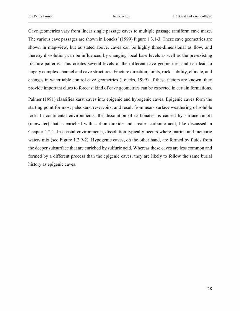
Cave geometries vary from linear single passage caves to multiple passage ramiform cave maze.
The various cave passages are shown in Loucks´ (1999) Figure 1.3.1-3. These cave geometries are
shown in map-view, but as stated above, caves can be highly three-dimensional as flow, and
thereby dissolution, can be influenced by changing local base levels as well as the pre-existing
fracture patterns. This creates several levels of the different cave geometries, and can lead to
hugely complex channel and cave structures. Fracture direction, joints, rock stability, climate, and
changes in water table control cave geometries (Loucks, 1999). If these factors are known, they
provide important clues to forecast kind of cave geometries can be expected in certain formations.
Palmer (1991) classifies karst caves into epigenic and hypogenic caves. Epigenic caves form the
starting point for most paleokarst reservoirs, and result from near- surface weathering of soluble
rock. In continental environments, the dissolution of carbonates, is caused by surface runoff
(rainwater) that is enriched with carbon dioxide and creates carbonic acid, like discussed in
Chapter 1.2.1. In coastal environments, dissolution typically occurs where marine and meteoric
waters mix (see Figure 1.2.9-2). Hypogenic caves, on the other hand, are formed by fluids from
the deeper subsurface that are enriched by sulfuric acid. Whereas these caves are less common and
formed by a different process than the epigenic caves, they are likely to follow the same burial
history as epigenic caves.

Jon Petter Furnée 1 Introduction 1.3 Karst and karst collapse
29
1.3.2 Paleokarst James and Choquette (1988) defines paleokarst as ancient karst. Loucks (1999) however defines
paleokarst as karst systems that are no longer active. The latter provides a more precise description,
as it specifies that the system is not only ancient, but also has to be inactive. Similarly Paleocave
systems are defined as cave systems that are no longer physically related in time and or space to
any active karst process that formed them (Loucks, 1999). This de-activation of the karst-forming
processes can be caused by physical isolation, cessation of processes and burial which over time
causes infill, collapse, compaction and mineralization. However, paleokarst systems may be re-
activated and karst features often exhibit patterns of more than one karstification event (see Figure
1.3.3-2).
De-activation of the karst forming process is commonly followed by infilling of cavities by a wide
range of sediments and cements. Loucks (1999) proposed a compositional classification scheme
for cave infills (Figure 1.3.2-1). In this system, cave infill is classified according to its mixture of
three end-member components: crackle breccia, chaotic breccia, and cave sediment.
Figure 1.3.2-1 Cave infill classification from (Loucks, 1999)

Jon Petter Furnée 1 Introduction 1.3 Karst and karst collapse
30
Breccias are commonly associated with paleokarst. They typically form due to fracturing, stoping
and collapse of caves, and commonly consist of angular clasts of the host rock with maximum
clast sizes corresponding the spacing of fracture patterns in the host rock. Breccias can be classified
according to the degree of internal displacement between clasts: crackle breccia show only minor
displacement between clasts, and essentially represent pervasively fractured host rock. Mosaic
breccia exhibit more displacement between clasts, but blocks can still be fitted together like a
puzzle; chaotic breccia consist of jumbled blocks. The latter may contain evidence of having been
subjected to transport and could include exotic clasts originating from collapse of overlying
formations or from lateral transport into the cave. The composition and amount of matrix material
in all these breccias may vary.
Paleokarst features are intimately linked to the karst features present at the time the karst process
becomes inactive. Paleokarst systems are therefore likely to inherit some geometrical properties
from the pre-existing karst system. Understanding the modern karst systems can therefore give
important clues to understanding paleokarst systems, in particular with respect to karst formation,
scale relationships, geometries and how their spatial distribution is linked to host rock lithology
and structural geology.

Jon Petter Furnée 1 Introduction 1.3 Karst and karst collapse
31
1.3.3 Burial and diagenesis of paleokarst Paleokarst systems are most commonly products of near-surface processes of karstification, with
later burial and compaction. They form an important class of hydrocarbon reservoirs. Loucks
(1999) states that while karst systems are well-studied; they are commonly not integrated into
paleokarst studies. Paleocave data is limited to outcrop and well data, but burial evolution can be
deciphered by comparing modern examples with different stages of ancient ones. Well-exposed
outcrops are rare, and the spatial organization of the ancient cave system is difficult to establish
even when using geophysical methods and well data, which in many cases can be difficult to
interpret or lack sufficient spatial resolution to allow detailed reconstruction to be made. (Loucks,
1999)
Outcrops and well data only show parts of the system, but do not provide the full picture with
respect to geometry and properties. Therefore, to get an impression of the 3-dimensional geometry,
it is necessary to look at modern cave systems and use them as proxies. For karst, like carbonates,
the term “The present is the key to the past” discussed earlier, refers more to the process than the
result. Basically, every cave system in carbonate rocks is formed by the same, limited set of
processes, but the resulting geometry differs due to local factors such as stress direction fractures
and faults in the rock hosting cave formation, and the level of the transition zones where caving
occurs. (Scholle and Scholle, 2014, Loucks, 1999).
Loucks (1999) shows a conceptual evolution of a single cave passage from its formation in the
near-surface phreatic zone to its collapse during burial (Figure 1.3.3-1). The figure is based on a
falling base level e.g. the cave system “moves” from the phreatic into the vadose zone. Loucks
(1999) further explains that breakout domes, like the one shown in the figure, commonly form
when base level drops. This because water supports 40% of the ceiling weight (White and White,
1969). When this support is lost, as water is drained out of the cave, ceiling and walls may collapse.
From the collapse follows infill of chaotic breakdown breccia inside the former phreatic tube.
Since the cave is collapsing, overlying strata tend to fracture, fault and sag downwards. During
burial, the former tube gets filled with all sorts of breccia types and cave sediment infill (se Figure
1.3.2-1 above). A halo of crackle breccia surrounds the former cave passage as a result of stress
relief in overlaying strata. As shown in Figure 1.3.1-2, compaction-related structures tend to
radiate beyond the circumference of the cave passage. This produces a larger body of rock with

Jon Petter Furnée 1 Introduction 1.3 Karst and karst collapse
32
enhanced permeability than if just the former phreatic tube was filled with sediment. It is obvious
that the former volume of the cave becomes distributed as pore space the new volume of breccia
if no compaction has taken place. The collapse stops when the former cave is completely filled
with cave infill.
Figure 1.3.3-1– Collapse of paleocave system from (Loucks, 1999) modified after (Loucks and Handford, 1992)

Jon Petter Furnée 1 Introduction 1.3 Karst and karst collapse
33
The complexity observed in formations exhibiting paleokarst, in particular with respect to
paleokarst formations being the result of multiple processes, can be illustrated by an example from
a Paleozoic limestone succession in Billefjorden, Svalbard. The photographs below, clearly
illustrate how cave infill (B2) can occur inside an older cave collapse breccia (B1). Furnée (2013)
states that the interesting part of this location is the perfect indication that there has been more than
one event of cave formation and collapse.
Figure 1.3.3-2 Cave infill in cave collapse breccia. Note breccia B2 in B1. Jan Tveranger as scale. Photo: Jon Petter Furnée. Figure modified from (Furnée, 2013)

Jon Petter Furnée 1 Introduction 1.3 Karst and karst collapse
34
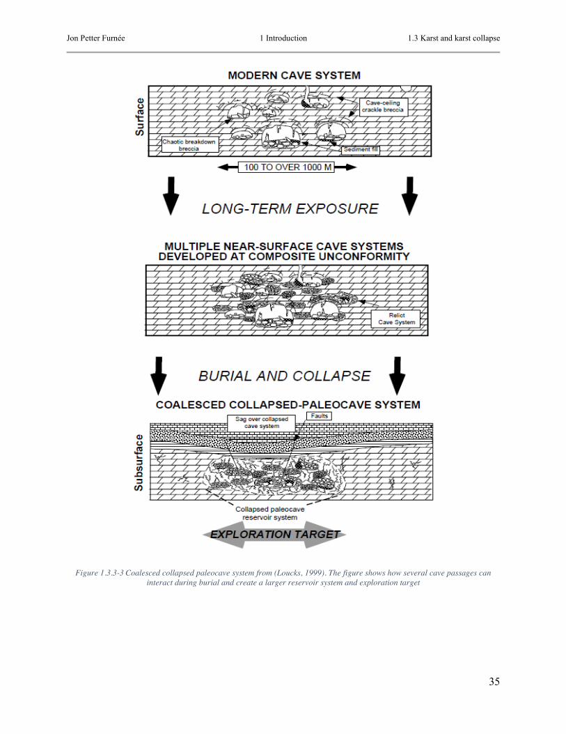
Loucks (1999 and 2007) claimed that most paleocave reservoirs are not products of isolated
collapsed passages but rather products of coalesced collapsed paleocave systems. These systems
can be several thousands of meters long and across. This is an important concept because it shows
that exploration targets on collapsed paleokarst reservoirs are likely to be much larger than
individual cave systems, and likely to be connected through fractures systems. Figure 1.3.3-3
shows a schematic diagram of the evolution of coalesced collapsed paleocave systems. These
systems develop as a result of several stages of development. As the multi-cave system subsides,
wall- and ceiling rock collapses, and may intersect with fractures from other collapsed passages
and older breccia’s within the system. Loucks (1999) and several other authors (Loucks and
Handford, 1992, Hammes, 1996, Mazzullo and Chilingarian, 1996, Kerans, 1988) explain that the
result of this process gives a spatially complex reservoir system, and a much larger exploration
target, than a single phreatic tube. Since the spatial complexity ranges from pore level to regional
scale, qualification becomes difficult. The overall pattern of spatial complexity is controlled by
original cave geometry and the number of cave passages. The distribution of porosity is controlled
by distribution of cave-sediment fill. The original areal extent of rock with porosity and
permeability enough to support fluid flow increases as the system collapses and fractures the rock
around the former passages. In addition, cementation during burial may totally change and reduce
porosity of the system. The final porosity and permeability is highly complex and spatially
variable. Loucks (1999) concludes that karst-related paleocave systems represent an important
class of carbonate petroleum reservoirs, and understanding their origin and burial history helps in
exploring and developing these reservoirs. Stein-Erik Lauritzen (2015, pers. comm., 28 April), on
the other hand, casts doubts on Loucks´ (1999) idea of coalesced collapsed paleocave systems.
The doubts are based on observations of the strength of perforated metal plates, where the metal
plates become stronger with holes. He further claims that isolated cave systems, do not merge into
one big breccia body as easily as Loucks´ (1999) describes, because the system becomes stronger
for each cave (up to a certain point) as for the metal plate.
Jon Petter Furnée 1 Introduction 1.3 Karst and karst collapse
35
Figure 1.3.3-3 Coalesced collapsed paleocave system from (Loucks, 1999). The figure shows how several cave passages can interact during burial and create a larger reservoir system and exploration target

Jon Petter Furnée 1 Introduction 1.3 Karst and karst collapse
36
1.3.4 Cave collapse model The collapse of a cave can be expressed as an increase of its initial cross-sectional radius. A simple
geometric approach is carried out by an equation (see equation (1) below) derived from Stein-Erik
Lauritzen (2014, pers. comm., 12 September). If the host rock is considered otherwise non-porous,
and no compaction is taking place, the total amount of pore space stays unchanged after collapse.
This initial porosity can be calculated based on the diameter of the cavities. As the cave collapses
the radius of the cavity increases, but the expanding cavity is simultaneously filled in with breccia.
Assuming that the collapse is evenly distributed along the caves periphery, the increase in radius
caused by collapse can be approximated as being equal to the inverse of the square root of the
porosity.
𝜋𝑅22 = 1
Ø𝜋𝑅1
2 Æ 𝑅22
𝑅12 = 1
Ø Æ 𝑅2
𝑅1= 1
ï (1)
Porosity, Ø, is expressed as a decimal fraction, and not in percent. 𝑅2 is radius after collapse, while
𝑅1 is radius before collapse. A complete list of symbols is presented in Appendix 7.1.4.
Se the Table 1.3.4-1 and its corresponding graph (Figure 1.3.4-1) for resulting values of the
calculation. The values marked with green color indicate the three cases for cave radius/porosity
selected as input to the reservoir models subjected to detailed study in this thesis. The radius after
collapse (R2) was initially set to be twice the radius of the original cave radius (R1). The other 𝑅2
values (12 and 14 meters) were introduced to test the effect of radius increase on the production
curves. For modeling simplicity the interval of 2 meters (10 → 12 → 14 meters) was used as the
initial grid has grid cells with dimension 2m × 2m × 2m.

Jon Petter Furnée 1 Introduction 1.3 Karst and karst collapse
37
Table 1.3.4-1 Table showing the relationship between resultant porosity (Ø) and R2/R1 in a collapsed cave. The green values are the three radius- and resulting porosity cases used as input in the reservoir model.
Figure 1.3.4-1 Plot showing the relationship between porosity (Ø) vs. R2/R1 in a collapsed cave. Values shown in green values in the table are the three cases used as input in the reservoir model.
Porosity, Ø R2/R1 R2
1.000 1.00 5.0
0.950 1.03 5.1
0.900 1.05 5.3
0.850 1.08 5.4
0.800 1.12 5.6
0.750 1.15 5.8
0.700 1.20 6.0
0.650 1.24 6.2
0.600 1.29 6.5
0.550 1.35 6.7
0.500 1.41 7.1
0.450 1.49 7.5
0.400 1.58 7.9
0.350 1.69 8.5
0.300 1.83 9.1
0.250 2.00 10.0
0.200 2.24 11.2
0.173611 2.40 12.0
0.150 2.58 12.9
0.127551 2.80 14.0
0.100 3.16 15.8
0.050 4.47 22.4
0.010 10.00 50.0

Jon Petter Furnée 1 Introduction 1.3 Karst and karst collapse
38
Figure 1.3.4-1 shows that if the radius of the cave is increased by a factor of two through collapse
(𝑅2 = 2 × 𝑅1), the cross-section area of the collapsed cavity is four times larger than that of the
initial cave (Area 2 = 4 × Area 1). If the initial cavity has a porosity of 100%, this translates into
an average porosity of 25% in the collapsed and infilled cave.
Figure 1.3.4-2 Conceptual cross sectional view of cave before (A1) and after collapse (A2) R1 and R2 are the radii of the cavity
before and after collapse, respectively. Note that the center of circle showing the cave after collapse is shifted upward to maintain the position of the cave floor.
This approximation can be further improved: Collapse is a gravity-driven process; thus brecciation
and gravity-driven expansion of the cave will not affect the initial cave floor. In order to provide
a reasonable approximation of the resulting geometry of the collapsed cave, the center point of the
collapse has to be moved R2-R1 up to maintain the same cave floor before and after collapse (see
Figure 1.3.4-2).
The porosity of the breccia filling the collapsed cavity is not likely to be homogeneously
distributed. For a collapsed cave filled purely by locally derived breccia, it is reasonable to assume
a general trend with the highest porosity values near the position of the initial cavity and decreasing
toward the margin of the collapse dome where it may show a gradual transition from inter-particle
porosity to fracture porosity (e.g. Kerans (1988), Nordeide (2008), see Figure 1.3.3-1 and Figure
1.3.4-3). However, different porosity patterns and trends can be expected if the cave is filled by

Jon Petter Furnée 1 Introduction 1.3 Karst and karst collapse
39
cements and/or allochtonous sediments, in particular as larger pore spaces in the initial collapse
breccia get filled-in by more fine-grained sediments.
Figure 1.3.4-3 Core and well logs showing a cave-infill/collapse succession from the Ellenburger Group, western Texas (Kerans, 1988)

Jon Petter Furnée 1 Introduction 1.3 Karst and karst collapse
40
1.3.5 Compaction of collapsed cave model Burial induces a vertically oriented pressure on the collapsed caves, and may cause additional
fracturing, porosity reduction of the cavity infill and pressure solution/recementation. It may also
conceivably change the overall geometry of the collapsed cave cross-section by flattening it; in
particular if the cave is not completely filled by prior to compaction. The extent of these effects is
closely linked to the mechanical strength of the host rock as well as burial depth, and needs to be
considered when performing porosity calculations along the lines suggested in the preceding
section. The effect of compaction is dependent on the time of occurrence. If the collapse occurs
early during burial, the effect of compaction on the collapse geometry is greater than if it occurs
late. For the porosity estimates employed in the models constructed as part of the present study,
the impact of compaction has not been included.
The width of the collapsed cave will be little affected by the compaction. If the host-rock is a
limestone with little porosity, compaction will be minor. If the host rock is a porous limestone, the
compaction can be significant. The former is the more likely case, as cave systems are more prone
to develop in rocks with low initial porosity.
However, none of the tools used in this study (see Chapter 1.4.2) include modules for explicit
handling of compaction. There are dedicated rock-mechanical modeling tools (e.g. VISAGE by
V.I.P.S and Eclipse Geomechanics by Schlumberger) some of which offer coupled flow and
mechanical modeling. Simulation times for these are typically one to three orders of magnitude
longer than pure fluid flow simulation, and they are generally not employed as part of the standard
industrial modeling workflow. (Doornhof et al., 2006).
Based on these considerations compaction effects are not included in the present modeling study.

Jon Petter Furnée 1 Introduction 1.4 Modeling and simulation of paleokarst reservoirs
41
1.4 Modeling and simulation of paleokarst reservoirs
1.4.1 Previous work The architectural and petrophysical complexity of collapsed karst systems make them very
challenging to model. Providing realistic geo-models which can serve as a reliable input to
forecasting production behavior is tricky because a range of processes are involved in the
formation of such systems. Some of these have been addressed by previous workers.
Pardo-Igúzquiza et al. (2011, 2012) and Collon-Drouaillet et al. (2012) show different approaches
to capture cave networks. Pardo-Igúzquiza et al. (2011) analyzes three-dimensional networks of
karst conduits, while Pardo-Igúzquiza et al. (2012) builds further with stochastic simulations of
these features. Collon-Drouaillet et al. (2012) stresses the fact that simulation of three-dimensional
karstic networks is required to build realistic carbonate reservoir models. The paper focuses on
branchwork karst, and how to simulate such networks with realistic, geologically consistent
geometries.
Several oral presentations hosted by AAPG (Feazel, 2010, Xiaoqiang et al., 2012) show ways of
modeling paleokarst reservoirs. Xiaoqiang et al. (2012) presents 3D modeling of the Tahe oil field
in China, which, as mentioned in the introduction (Chapter 1), is a paleokarst reservoir. The model
is based on a geostatistical analysis of karst geology as well as probability from both well and
seismic. Feazel (2010) presents the use of modern cave systems as analogs for paleokarst systems,
and illustrates that cave surveys can be used to assign properties in geocellular models of karsted
reservoirs. Feazel (2010) further presents examples for seismic forward modeling and seismic
velocity models with different sensitivities with respect to cave size and cave infill.
Petrophysical properties in carbonate rocks and collapse breccia is among others described by
Lønøy (2006), Lucia (1995, 2004, 2007), and Loucks (1999, 2007). They all specify the
complexity in these rocks, and describe the wide range of petrophysical values within the different
cases. Lønøy (2006) is used in this thesis to assign average permeability to different porosity cases.
Studies related to flow behavior in paleokarst reservoirs have been carried out by former master
students at Uni CIPR (Centre for Integrated Petroleum Research). Common for them all, is the
vertical breccia pipe aspect of paleokarst.

Jon Petter Furnée 1 Introduction 1.4 Modeling and simulation of paleokarst reservoirs
42
Nordli (2009) investigated the impact of breccia pipe features on fluid flow behavior in a reservoir
setting and assessed their relative influence. The study lists the factors that are most important to
include in reservoir models where breccia pipes are present. Nordli (2009) based the geological
input to the reservoir models on Nordeide (2008) who quantified several properties of collapse
breccia in the Wordiekammen formation (Billefjorden, Svalbard). Nordli (2009) stresses the
importance of including breccia pipes in reservoir models if present, or even suspected. “The most
significant factor affecting fluid flow was found to be the magnitude of permeability contrast
between the pipe and background... an increased permeability contrast will result in poorer sweep
of the background volume and enhanced flow of fluids through the pipe.” (Nordli, 2009). Further
Nordli (2009) states that if the reservoir model includes high permeable beds in background
(structural subdivision of layers), fluids will be “lost” in these layers, resulting in poorer sweep.
Nordli (2009) hereby confirms the suggestion made by Nordeide (2008), that permeable beds in
background has a significant impact on fluid flow.
Dalva (2012) expanded on Nordli´s (2009) thesis by presenting a reservoir with pipes present, and
investigating if the presence of breccia pipes in a reservoir could be deduced from observed
production behavior. One of his major conclusions in addition to the evidence that pipes were
present in the system, was that “The breccia pipe shape can be simplified to that of a square box
instead of a cylindrical (radial) shape, provided the breccia pipe volumes are kept equal.” (Dalva,
2012). This suggests that the impact of at least some paleokarst features on production can be
captured even if some simplifications are employed in the modeling.
Jon Petter Furnée 1 Introduction 1.4 Modeling and simulation of paleokarst reservoirs
43
1.4.2 Introduction to the software Reservoir models are primarily used for visualizing, integrating and analyzing all available
datasets from subsurface reservoirs, and serve as common platforms for linking geology,
geophysics, petrophysics and reservoir engineering. The integration and analysis of data coupled
to geological know-how and the laws of physics make them powerful tools for forecasting
reservoir properties, calculating volumes and predicting their dynamic behavior over time. Thus
reservoir models are key tools for hydrocarbon exploration and production; identifying prospects
and ensuring safe, optimized and financially sound field management.
The geo-modeling was performed using RMSTM 2013 by Roxar Software Solutions; a standard
industrial reservoir modeling tool. For flow simulations Eclipse 2013.2; a reservoir simulation tool
by Schlumberger was employed. For creating a fracture rose based on cave directions, GeoRose
0.4.0, designed by Yong Technology Inc. was used.
According to Pettersen (2006) reservoir simulators "…simulate the exploitation of a real reservoir
without the costs of real life trial and error, e.g. to test different productions scenarios to find an
optimal one before the reservoir is actually put on production". Eclipse does this by solving
numerous dynamic equations on a discretized (gridded) 3D rendering of a body of rock/reservoir
populated with relevant properties, providing an accurate prediction of dynamic behavior for all
types of reservoirs. (Schlumberger, 2014b).
However, "an accurate prediction" still comes with attached uncertainties, in particular if geology
is involved. Forecasting-precision is mainly dependent on the accuracy of input parameters, but
software implementation aspects such as grid resolution and the manner in which geological
structures and properties are rendered may also affect results. Deterministic reservoir models,
involving a fixed input and a single outcome (realization) are therefore of limited use if input
parameters are poorly constrained. To overcome this problem reservoir models employ stochastic
methods which generate a range of possible outcomes (realizations) weighed by the likelihood or
probabilities of a given set of circumstances. The resulting spread of outcomes reflects uncertainty
of the forecast.
The present study focuses on the impact of certain modeling parameters on reservoir performance.
Thus, although stochastic modeling is the most commonly used method in “real life” settings, we

Jon Petter Furnée 1 Introduction 1.4 Modeling and simulation of paleokarst reservoirs
44
here employ sets of deterministic models in order to retain full control of the input parameters and
subsequent simulation outcomes.
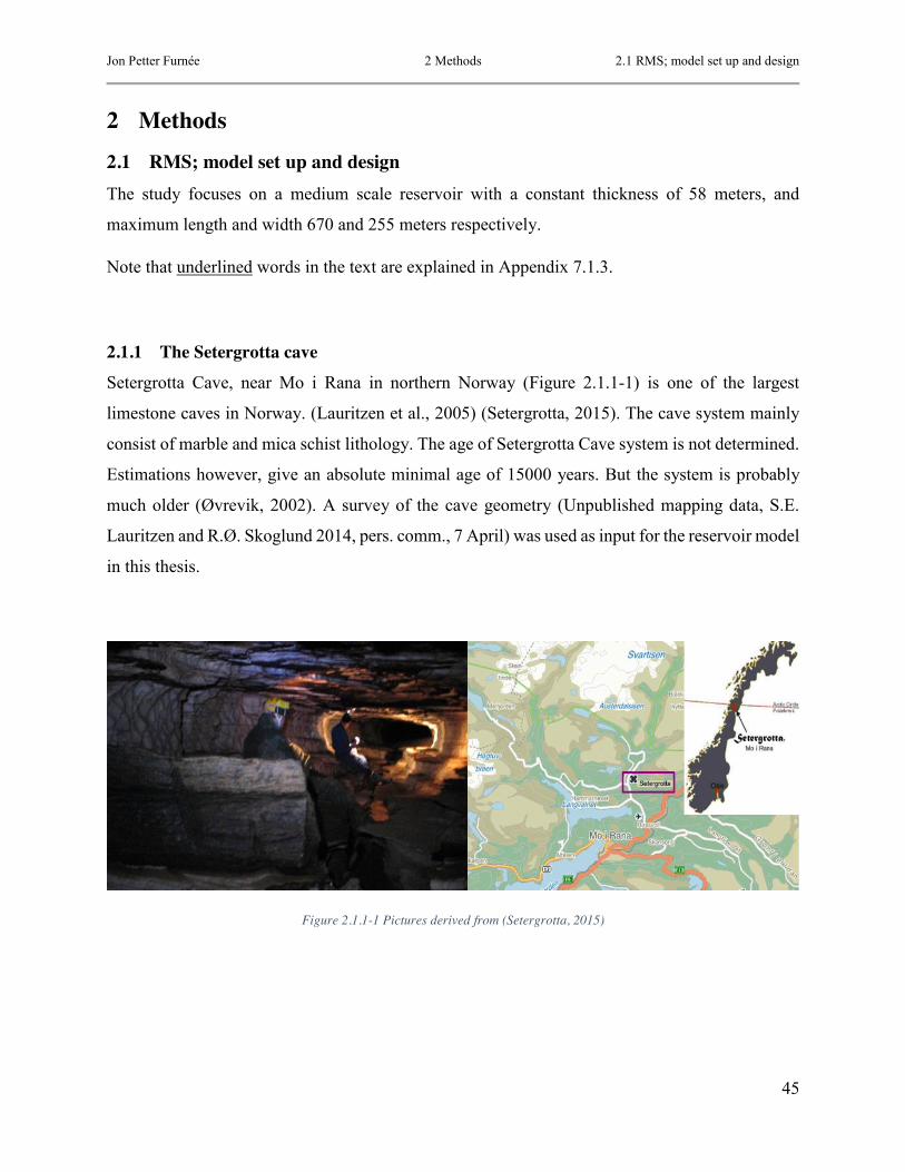
Jon Petter Furnée 2 Methods 2.1 RMS; model set up and design
45
2 Methods 2.1 RMS; model set up and design The study focuses on a medium scale reservoir with a constant thickness of 58 meters, and
maximum length and width 670 and 255 meters respectively.
Note that underlined words in the text are explained in Appendix 7.1.3.
2.1.1 The Setergrotta cave Setergrotta Cave, near Mo i Rana in northern Norway (Figure 2.1.1-1) is one of the largest
limestone caves in Norway. (Lauritzen et al., 2005) (Setergrotta, 2015). The cave system mainly
consist of marble and mica schist lithology. The age of Setergrotta Cave system is not determined.
Estimations however, give an absolute minimal age of 15000 years. But the system is probably
much older (Øvrevik, 2002). A survey of the cave geometry (Unpublished mapping data, S.E.
Lauritzen and R.Ø. Skoglund 2014, pers. comm., 7 April) was used as input for the reservoir model
in this thesis.
Figure 2.1.1-1 Pictures derived from (Setergrotta, 2015)

Jon Petter Furnée 2 Methods 2.1 RMS; model set up and design
46
2.1.2 2D data and skeleton lines To create a realistic cave geometry for further modeling and simulation of paleokarst reservoirs,
survey points from Setergrotta Cave were used. These were imported to RMS as general 2D data
points. The survey data include center-, wall-, floor-, and ceiling points given as local XYZ-
coordinates (Unpublished mapping data, S.E. Lauritzen and R.Ø. Skoglund 2014, pers. comm., 7
April). In order to remove any negative coordinate values, the values were multiplied with (-1) and
500 meters was added to all points. This was done in Excel before importing the points as .txt-
format.
In Clipboard an empty polygon was created, and used to analyze the path between the center points
of the survey. This polygon was named SkeletonLines, and added to the General 2D data. The
points for wall, floor, and ceiling, were only used to understand the geometry of the cave. See
Figure 2.1.2-1.
Figure 2.1.2-1 SkeletonLines polygon based on input measure points (Unpublished mapping data, S.E. Lauritzen and R.Ø. Skoglund 2014, pers. comm., 7 April) from Setergrotta Cave.

Jon Petter Furnée 2 Methods 2.1 RMS; model set up and design
47
In order to provide a more realistic depth for later flow simulation, 1518 meters was added to the
z-coordinates of the SkeletonLines, so that the depth range of the new SkeletonLines2000 is 2000-
2071 meters below mean sea level, therefore the name SkeletonLines2000.
SkeletonLines2000 is based on a 3D point dataset of a multistoried cave passage. The starting point
for further surface mapping was done by adapting the depth trend of the SkeletonLines2000 to a
boundary as described in the next chapter.

Jon Petter Furnée 2 Methods 2.1 RMS; model set up and design
48
2.1.3 Stratigraphic framework and horizon mapping Three horizons where defined to serve as input to the structural framework and later used to create
a horizon model (Chapter 2.1.4).
Cave_top
Cave
Cave_bottom
All with Type as Interpreted Horizon. The SkeletonLines2000 polygon was dropped on top of
SkeletonLines under the horizon Cave. No faults are included in the model.
In order to map the Cave_top and Cave_bottom horizons; representing the top and bottom of the
stratigraphic interval included in the model, DepthPoints are needed. To create these, the easiest
way was to make a copy of the SkeletonLines2000 from horizon Cave in Clipboard, right click
and select create boundary. The resulting polygon (BoundarySkeletonLines2000) outlines the
areal extent of the model. This polygon was slightly adjusted to avoid intersection points between
the boundary and the SkeletonLines2000. This space is essential to build a grid with background
in addition to the cave structure. See Figure 2.1.3-1.
Figure 2.1.3-1 Boundary (BoundarySkeletonLines2000) of cave model. Notice the adjustments made so that the boundary leaves some space for the SkeletonLines. This space is essential to build a grid with background in addition to the cave structure.

Jon Petter Furnée 2 Methods 2.1 RMS; model set up and design
49
Two copies of the boundary were made in Clipboard, Boundary43up and Boundary27down. These
were adjusted respectively to 43 meters up and 27 meters down from BoundarySkeletonLines2000.
As a result, all of the center points of the cave fell within the framework of these boundaries (see
Figure 2.1.3-2). The boundaries were dragged and dropped onto DepthPoints for Cave_top and
Cave_bottom under Horizons, and used as input for horizon mapping.
Figure 2.1.3-2 Boundary43up (red), Boundary27down (blue) and BoundarySkeletonLines2000 (purple) which is based on the SkeletonLines2000 (orange).
Horizon mapping was carried out for the Cave_top and Cave_bottom. The inputs were the
DepthPoints created by the boundaries above, and the outputs were DepthSurface. See Figure
2.1.3-3 for the horizons. The default algorithm “Local B-spline” was used for mapping the
horizons. It gives good results for all types of mapping, and does not require any user-defined
settings (Roxar, 2013b). The polygons were used to constrain the areal extent of the horizons.

Jon Petter Furnée 2 Methods 2.1 RMS; model set up and design
50
Figure 2.1.3-3 Horizons Cave_top and Cave_bottom with Boundary43up (red), Boundary27down (blue) and BoundarySkeletonLines2000 (purple) which is based on the SkeletonLines2000 (orange).
These two horizons define the top and base of the reservoir model and serve as base for the
structural modeling, horizon modeling and subsequent grid-building.

Jon Petter Furnée 2 Methods 2.1 RMS; model set up and design
51
2.1.4 Structural model and horizon modeling To create a grid, it is necessary to have a horizon model. A structural model Cave was made, and
a model box was defined based on the spatial range from object BoundarySkeletonLines2000, with
adjusted XYZ-length. A horizon model Cave2000 was made based on the structural model and the
horizons Cave_top and Cave_bottom from Chapter 2.1.3.
Table 2.1.4-1 Box definition based on the range from object BoundarySkeletonLines2000, with adjusted XYZ-length
Centre Length
X 475.90 500.00
Y 394.46 750.00
Z 2036.75 170.00
Selected horizons were:
Figure 2.1.4-1 Horizons in horizon model Cave2000. Compare to the structure in Figure 2.1.4-2 and Figure 2.1.4-3.
The input data types were the DepthSurfaces described above. The resolution and increment in
XY-direction was set to 1 meter. The outputs from the structural modeling are the horizons
Cave_top and Cave_bottom in Figure 2.1.4-2 and the horizon model in Figure 2.1.4-3.

Jon Petter Furnée 2 Methods 2.1 RMS; model set up and design
52
Figure 2.1.4-2 Horizons Cave_top and Cave_bottom
The body of rock “Cave” in blue in Figure 2.1.4-3 is used to create a reservoir grid model.
Figure 2.1.4-3 Horizon model Cave2000, based on horizons Cave_top and Cave_bottom. Note the blue section “Cave”. This is the body of rock between these two horizons delimiting the spatial extent of the reservoir grid.

Jon Petter Furnée 2 Methods 2.1 RMS; model set up and design
53
2.1.5 Grid models A grid model called Grid2000_2_10_high (see Appendix 7.1.1 for explanation of the Grid model
names) was created, with horizon model Cave2000 as input. Under 2D layout, the grid was clipped
using the BoundarySkeletonLines2000 polygon, to save number of grid cells (see Figure 2.1.5-1).
The grid is rotated by 15 degrees to adapt it to the structural trend and lineaments evident from the
cave structure (see Chapter 2.1.8). Then Auto-calculate best fit option was selected, and grid
dimensions were set to an increment of 2 meters in x- and y-direction. Under Zone layout number
of cells was set to be 35. This because the grid is built between the Cave_top and Cave_bottom
surfaces which were adjusted respectively to 43 meters up and 27 meters down from the
BoundarySkeletonLines2000 (see Chapter 2.1.3). This equals a total thickness of 70 meters, and to
get an increment of 2 meters in z-direction, number of cells is set to be 70 2⁄ = 35 cells. The grid
consists of 1323735 grid cells with cell dimensions 2m × 2m × 2m. Total reservoir volume is
1323735 × 2 × 2 × 2 m3 ≈ 10.6 MSm3.
Figure 2.1.5-1 Left picture shows Cave in horizon model Cave2000. This volume defines the region to be gridded. To the right is the resulting grid model Grid2000_2_10_high that is clipped outside the polygon BoundarySkeletonLines2000 to save number of
cells. Grid2000_2_10_high has grid diameter of 2 meters.

Jon Petter Furnée 2 Methods 2.1 RMS; model set up and design
54
2.1.6 Geometric modeling The Geometric modeling functionality in RMS was used to implement and visualize the cave
passages inside the grid. This functionality allows the definition and calculation of distance to a
given point, well or surface. It was not possible to use the SkeletonLines as an input object directly.
Therefore, points based on the SkeletonLines2000 were made by refining the segments between
the initial center points. This was carried out by selecting all lines in the 3D window and clicking
on refine selected segments until the points were as close as needed to not lose any information or
get gaps while gridding. After refining the lines/polygon, empty points were created in the
Clipboard and the refined SkeletonLines2000 were dragged onto these. The
RefinedPoints_SkeletonLines2000, as they were named, could now be used as object in geometric
modeling. A geometric model, Geometric_5 was generated. When selecting calculation type
Distance to objects, the cell values increase for each meter from the centerline. See Figure 2.1.6-1
below.
Figure 2.1.6-1 Geometric model (Geometric_5) measuring distance from the centerline of the cave (RefinedPoints_SkeletonLines2000). Blue is near, and red far away from the centerline.
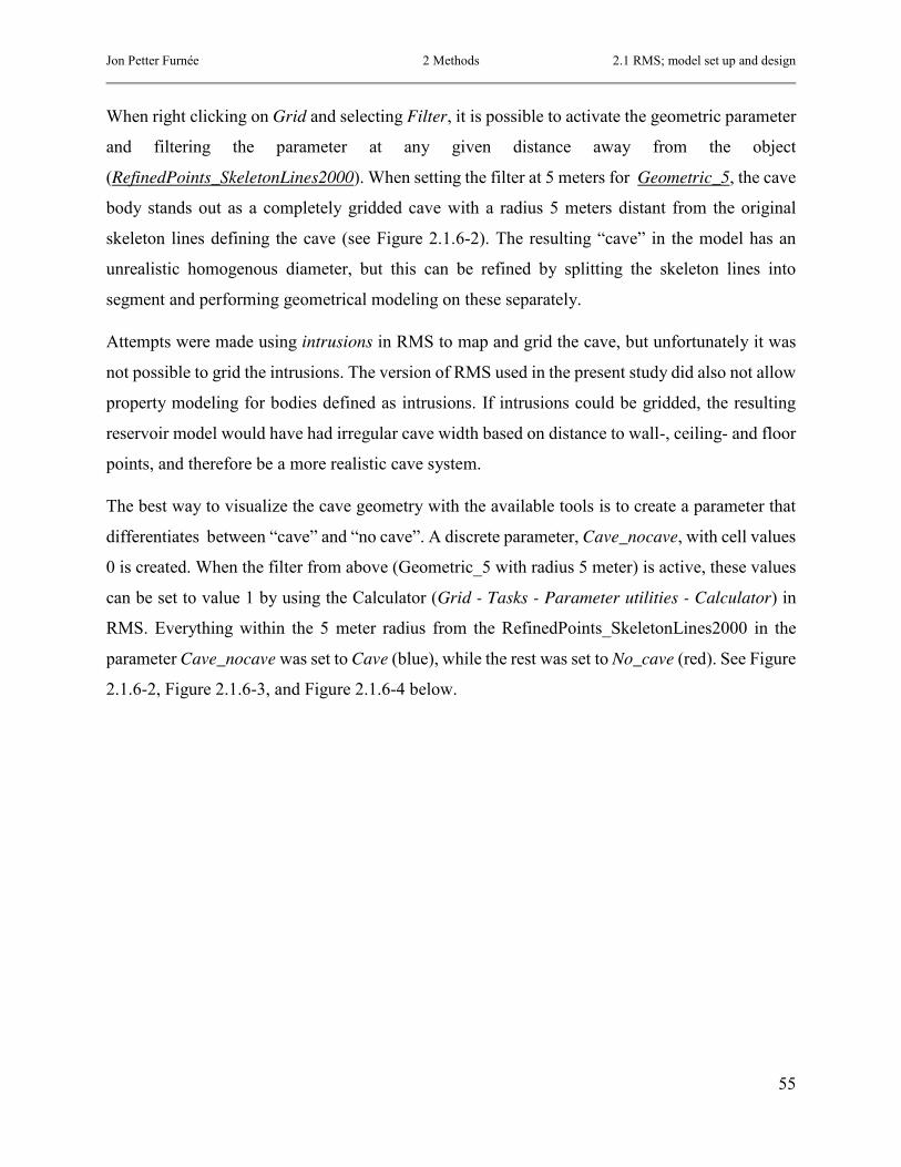
Jon Petter Furnée 2 Methods 2.1 RMS; model set up and design
55
When right clicking on Grid and selecting Filter, it is possible to activate the geometric parameter
and filtering the parameter at any given distance away from the object
(RefinedPoints_SkeletonLines2000). When setting the filter at 5 meters for Geometric_5, the cave
body stands out as a completely gridded cave with a radius 5 meters distant from the original
skeleton lines defining the cave (see Figure 2.1.6-2). The resulting “cave” in the model has an
unrealistic homogenous diameter, but this can be refined by splitting the skeleton lines into
segment and performing geometrical modeling on these separately.
Attempts were made using intrusions in RMS to map and grid the cave, but unfortunately it was
not possible to grid the intrusions. The version of RMS used in the present study did also not allow
property modeling for bodies defined as intrusions. If intrusions could be gridded, the resulting
reservoir model would have had irregular cave width based on distance to wall-, ceiling- and floor
points, and therefore be a more realistic cave system.
The best way to visualize the cave geometry with the available tools is to create a parameter that
differentiates between “cave” and “no cave”. A discrete parameter, Cave_nocave, with cell values
0 is created. When the filter from above (Geometric_5 with radius 5 meter) is active, these values
can be set to value 1 by using the Calculator (Grid - Tasks - Parameter utilities - Calculator) in
RMS. Everything within the 5 meter radius from the RefinedPoints_SkeletonLines2000 in the
parameter Cave_nocave was set to Cave (blue), while the rest was set to No_cave (red). See Figure
2.1.6-2, Figure 2.1.6-3, and Figure 2.1.6-4 below.

Jon Petter Furnée 2 Methods 2.1 RMS; model set up and design
56
Figure 2.1.6-2 Gridded cave (red) with a total of 26440 cells (2x2x2meters)
Figure 2.1.6-3 Gridded no_cave (purple) with cave (red) with a total of 1323735 cells. No_cave has 1297295 cells.
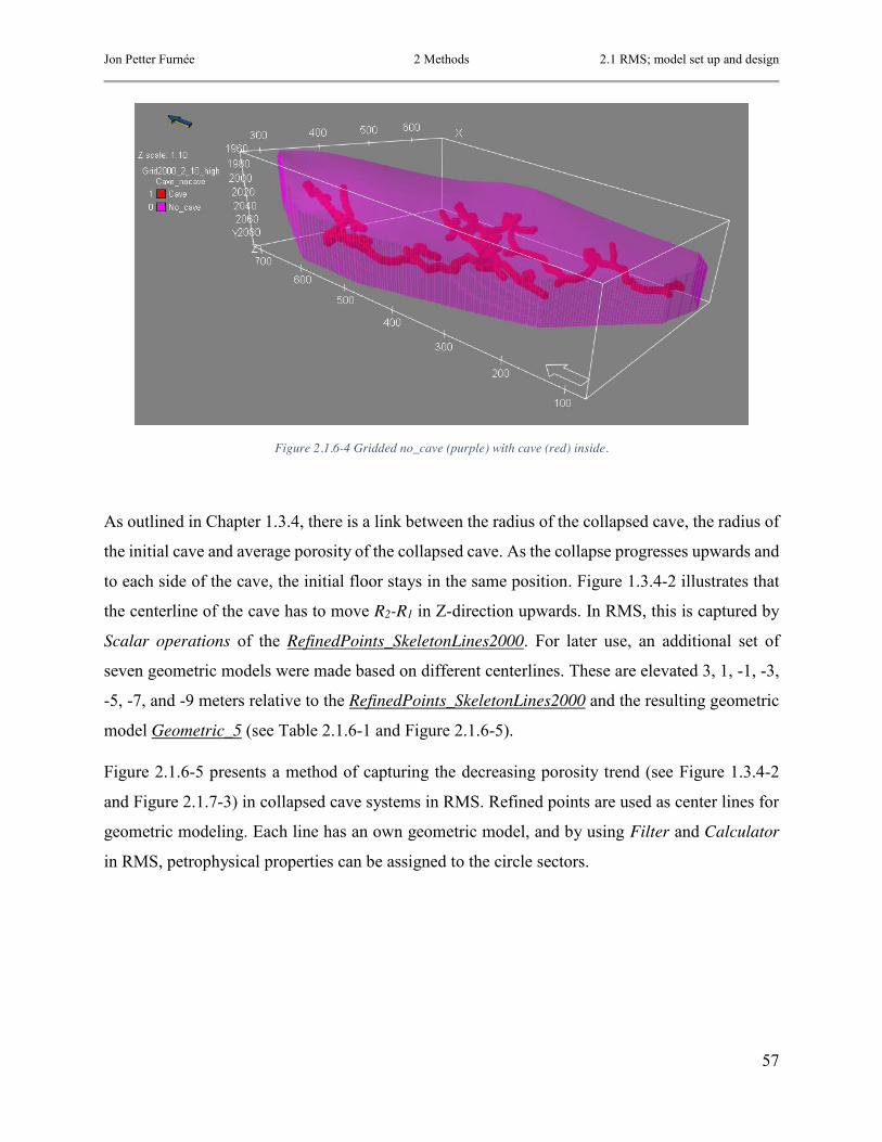
Jon Petter Furnée 2 Methods 2.1 RMS; model set up and design
57
Figure 2.1.6-4 Gridded no_cave (purple) with cave (red) inside.
As outlined in Chapter 1.3.4, there is a link between the radius of the collapsed cave, the radius of
the initial cave and average porosity of the collapsed cave. As the collapse progresses upwards and
to each side of the cave, the initial floor stays in the same position. Figure 1.3.4-2 illustrates that
the centerline of the cave has to move R2-R1 in Z-direction upwards. In RMS, this is captured by
Scalar operations of the RefinedPoints_SkeletonLines2000. For later use, an additional set of
seven geometric models were made based on different centerlines. These are elevated 3, 1, -1, -3,
-5, -7, and -9 meters relative to the RefinedPoints_SkeletonLines2000 and the resulting geometric
model Geometric_5 (see Table 2.1.6-1 and Figure 2.1.6-5).
Figure 2.1.6-5 presents a method of capturing the decreasing porosity trend (see Figure 1.3.4-2
and Figure 2.1.7-3) in collapsed cave systems in RMS. Refined points are used as center lines for
geometric modeling. Each line has an own geometric model, and by using Filter and Calculator
in RMS, petrophysical properties can be assigned to the circle sectors.

Jon Petter Furnée 2 Methods 2.1 RMS; model set up and design
58
Table 2.1.6-1 Additional Geometric Models for later calculation
Elevated refined points as input for geometric modeling
Geometric model Elevation from original RefinedPoints_SkeletonLines2000
RefinedPoints_SkeletonLines2000_+3 Geometric_2 3 meters
RefinedPoints_SkeletonLines2000_+1 Geometric_4 1 meter
RefinedPoints_SkeletonLines2000_-1 Geometric_6 -1 meter
RefinedPoints_SkeletonLines2000_-3 Geometric_8 -3 meters
RefinedPoints_SkeletonLines2000_-5 Geometric_10 -5 meters
RefinedPoints_SkeletonLines2000_-7 Geometric_12 -7 meters
RefinedPoints_SkeletonLines2000_-9 Geometric_14 -9 meters
Figure 2.1.6-5 This figure presents the method of capturing the decreasing porosity trend (see Figure 1.3.4-2 and Figure 2.1.7-3) in collapsed cave systems in RMS. Refined points (see Appendix 7.1.3 for explanation) are used as center lines for geometric
modeling. Each line has an own geometric model, and by using Filter and Calculator in RMS, petrophysical properties can be assigned to the circle sectors. Here porosity for Grid2000_2_10_high is presented.

Jon Petter Furnée 2 Methods 2.1 RMS; model set up and design
59
8 cases
5% background porosity
No cave
Radius 10 m, 25.00% porosity in collapsed cave
Radius 12 m, 17.36% porosity in collapsed cave
Radius 14 m, 12.76% porosity in collapsed cave
20% background porosity
No cave
Radius 10 m, 25.00% porosity in collapsed cave
Radius 12 m, 17.36% porosity in collapsed cave
Radius 14 m, 12.76% porosity in collapsed cave
2.1.7 Porosity and permeability in the reservoir model The determination of porosity and permeability values for use in a paleokarst reservoir model is
not straight forward. First of all, porosity values vary both between and within carbonate systems
as a result of their complexity (see Chapters 1.1.1 and 1.2.8). As mentioned in Chapter 1.2.8,
Brown (1997), Goldhammer (1997), and Schmoker and Halley (1982) describe different carbonate
systems and their porosity values plotted against depth. From these studies, carbonate systems like
grainstones seem to have a porosity varying between 5 and 20 % on a typical hydrocarbon reservoir
depth of 2000 meters (below mean sea level). This will be treated as minimum and maximum case
for the background porosity.
The porosity inside of the collapsed cave is dependent on the resulting radius of the collapsed cave
and sediment fill. As described in Chapter 1.3.4, the end radius after collapse (R2) for the three
cases in this thesis will be 10, 12, and 14 meters. These radii result in different average porosities
for the resulting collapsed cave. See below.
Table 2.1.7-1 Radius after collapse (R2) for the three cases in this thesis will be 10, 12, and 14 meters. These are the green values from Table 1.3.4-1.
R2 Ø %
10.0 25.00
12.0 17.36
14.0 12.76
Figure 2.1.7-1 This figure describes the eight cases for geometry and porosity/permeability in this thesis.

Jon Petter Furnée 2 Methods 2.1 RMS; model set up and design
60
As Figure 1.3.4-2 describes the geometry of the cave after collapse, Figure 2.1.7-3 shows how to
model such a feature in RMS. It shows a propagating collapse of the original cave structure, with
three end-cases based on the radius of the collapsed cave. The centerline has to be moved upwards
as Figure 1.3.4-2 and Table 2.1.6-1 shows, to keep the initial cave floor at a constant elevation.
Figure 2.1.7-2 illustrates a cave opening, and a potential cave collapse halo of cave roof and walls.
Figure 2.1.7-2 This picture illustrates a cave opening, and a potential cave collapse halo of cave roof and walls. Compare to
Figure 2.1.7-3.
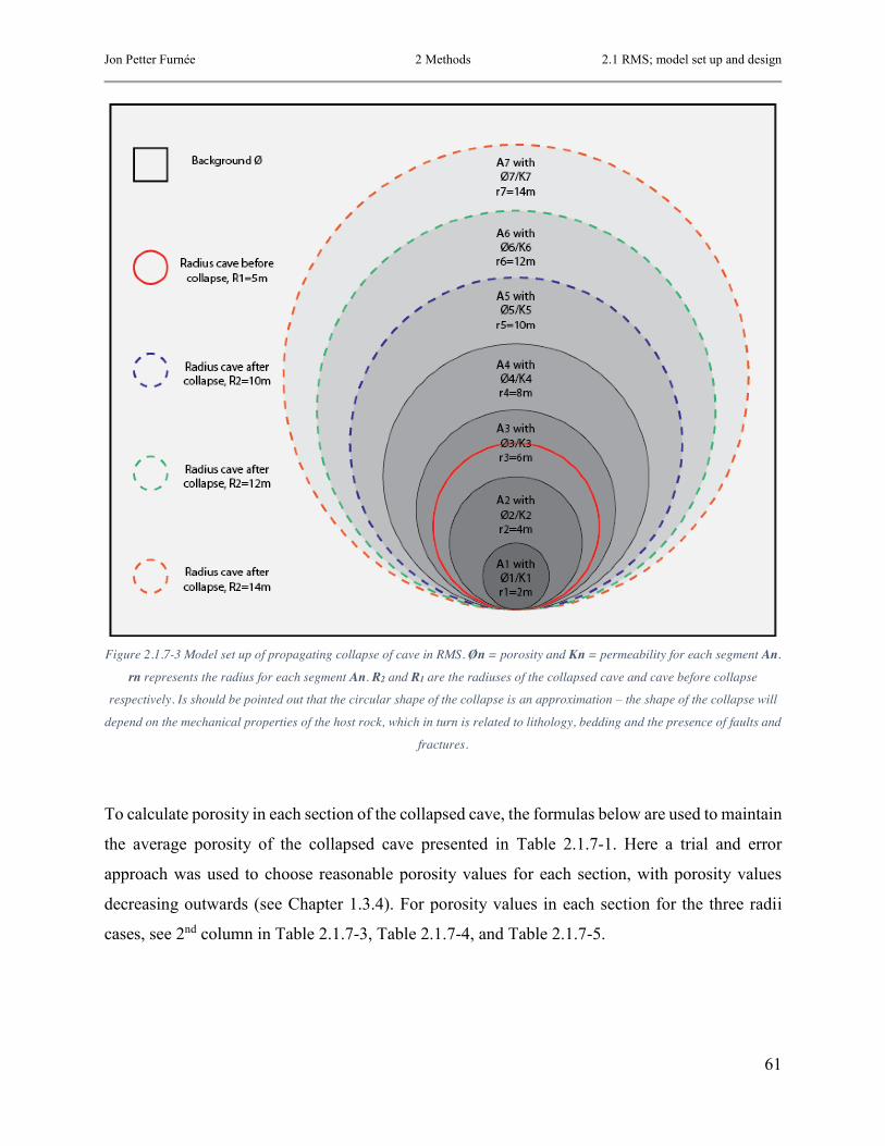
Jon Petter Furnée 2 Methods 2.1 RMS; model set up and design
61
Figure 2.1.7-3 Model set up of propagating collapse of cave in RMS. Øn = porosity and Kn = permeability for each segment An.
rn represents the radius for each segment An. R2 and R1 are the radiuses of the collapsed cave and cave before collapse
respectively. Is should be pointed out that the circular shape of the collapse is an approximation – the shape of the collapse will
depend on the mechanical properties of the host rock, which in turn is related to lithology, bedding and the presence of faults and
fractures.
To calculate porosity in each section of the collapsed cave, the formulas below are used to maintain
the average porosity of the collapsed cave presented in Table 2.1.7-1. Here a trial and error
approach was used to choose reasonable porosity values for each section, with porosity values
decreasing outwards (see Chapter 1.3.4). For porosity values in each section for the three radii
cases, see 2nd column in Table 2.1.7-3, Table 2.1.7-4, and Table 2.1.7-5.

Jon Petter Furnée 2 Methods 2.1 RMS; model set up and design
62
The formulae below ensure that the average porosity in the collapsed cave remains constant as in
Table 2.1.7-1. A complete list of symbols is presented in Appendix 7.1.4.
𝐴𝑛 × Ø𝑛 + ⋯ + 𝐴1 × Ø1 = 𝐴𝑡 × Ø𝑡 (2)
𝜋(𝑟𝑛2 − 𝑟𝑛−1
2) × Ø𝑛 + ⋯ + 𝜋(𝑟22 − 𝑟1
2) × Ø2 + 𝜋𝑟12 × Ø1 = 𝜋𝑟𝑡
2 × Ø𝑡 (3)
(𝑟𝑛2 − 𝑟𝑛−1
2) × Ø𝑛 + ⋯ + (𝑟22 − 𝑟1
2) × Ø2 + 𝑟12 × Ø1 = 𝑟𝑡
2 × Ø𝑡 = 2500 (4)
To calculate permeability for the host rock, in this case a grainstone a with porosity of 5 or 20 %,
the chart “Intercrystalline macroporosity” from Lønøy (2006) is used.
Figure 2.1.7-4 (Lønøy, 2006) Intercrystalline Macroporosity. Macropores are most common in moderately to wellsorted, high-
energy grainstones.
The formula gives permeability from porosity. A complete list of symbols is presented in Appendix
7.1.4.
𝑙𝑜𝑔(𝐾) = 1.399 × 𝐿𝑛(Ø) − 2.3081 (5)
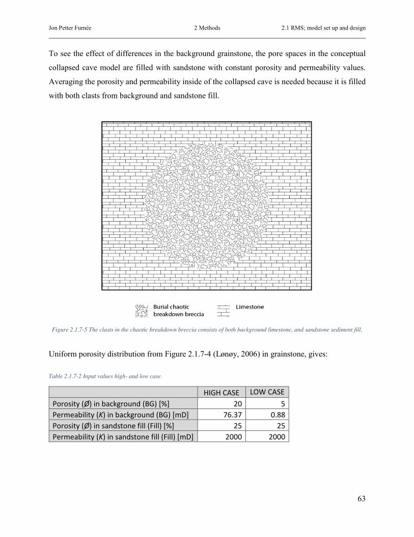
Jon Petter Furnée 2 Methods 2.1 RMS; model set up and design
63
To see the effect of differences in the background grainstone, the pore spaces in the conceptual
collapsed cave model are filled with sandstone with constant porosity and permeability values.
Averaging the porosity and permeability inside of the collapsed cave is needed because it is filled
with both clasts from background and sandstone fill.
Figure 2.1.7-5 The clasts in the chaotic breakdown breccia consists of both background limestone, and sandstone sediment fill.
Uniform porosity distribution from Figure 2.1.7-4 (Lønøy, 2006) in grainstone, gives: Table 2.1.7-2 Input values high- and low case
HIGH CASE LOW CASE Porosity (Ø) in background (BG) [%] 20 5 Permeability (K) in background (BG) [mD] 76.37 0.88 Porosity (Ø) in sandstone fill (Fill) [%] 25 25 Permeability (K) in sandstone fill (Fill) [mD] 2000 2000

Jon Petter Furnée 2 Methods 2.1 RMS; model set up and design
64
To average the porosity inside of the collapsed cave, arithmetic averaging is used. (Roxar, 2013a).
A complete list of symbols is presented in Appendix 7.1.4.
𝑃𝐴 = (∑ 𝑊𝑛𝑃𝑛n∑ 𝑊𝑛n
) (6)
Example:
Values from Table 2.1.7-2 (high case) and Table 2.1.7-3 (Area A1, high case, porosity).
Porosity (Ø) = (46×25 %+54×20 %46+54
) = 2230 %100
= 22.3 % (7)
Because of the chaotic nature of the system, geometric averaging is used for permeability. This
yields a value between arithmetic and harmonic average. (Roxar, 2013a). A complete list of
symbols is presented in Appendix 7.1.4.
𝑃𝐺 = exp (∑ 𝑊𝑛Ln𝑃𝑛n∑ 𝑊𝑛n
) (8)
Example:
Values from Table 2.1.7-2 (high case) and Table 2.1.7-3 (Area A1, high case, permeability).
Permeability (𝐾) = exp (46×Ln(2000 mD)+54×Ln(76.37 mD)46+54
) = e5.83764 = 342.97 mD (9)
See Table 2.1.7-3, Table 2.1.7-4, and Table 2.1.7-5 for complete calculation of porosity and
permeability values for each area in the six collapsed cave cases.

Jon Petter Furnée 2 Methods 2.1 RMS; model set up and design
65
Table 2.1.7-3 Radius collapsed cave (R2) = 10 Æ R2/R1 = 2.0 Æ Øt = 25.0 %. See Table 2.1.7-2 for explanations of BG and Fill
HIGH CASE LOW CASE Area Ø Fill [%] Ø BG [%] Tot. Ø [%] Tot. Perm [mD] Tot. Ø [%] Tot. Perm [mD]
A1 46.00 54.00 22.30 342.97 14.20 30.76 A2 39.00 61.00 21.95 272.89 12.80 17.90 A3 32.00 68.00 21.60 217.13 11.40 10.42 A4 20.00 80.00 21.00 146.74 9.00 4.12 A5 18.00 82.00 20.90 137.46 8.60 3.53 BG 0.00 100.00 20.00 76.37 5.00 0.88
Table 2.1.7-4 Radius collapsed cave (R2) = 12 Æ R2/R1 = 2.4 Æ Øt = 17.4 %. See Table 2.1.7-2 for explanations of BG and Fill
HIGH CASE LOW CASE Area Ø Fill [%] Ø BG [%] Tot. Ø [%] Tot. Perm [mD] Tot. Ø [%] Tot. Perm [mD]
A1 43.00 57.00 22.15 310.97 13.60 24.39 A2 38.00 62.00 21.90 264.12 12.60 16.57 A3 31.00 69.00 21.55 210.16 11.20 9.65 A4 20.00 80.00 21.00 146.74 9.00 4.12 A5 18.00 82.00 20.90 137.46 8.60 3.53 A6 1.00 99.00 20.05 78.91 5.20 0.95 BG 0.00 100.00 20.00 76.37 5.00 0.88
Table 2.1.7-5 Radius collapsed cave (R2) = 14 Æ R2/R1 = 2.8 Æ Øt = 12.8 %. See Table 2.1.7-2 for explanations of BG and Fill
HIGH CASE LOW CASE Area Ø Fill [%] Ø BG [%] Tot. Ø [%] Tot. Perm [mD] Tot. Ø [%] Tot. Perm [mD]
A1 41.00 59.00 22.05 291.31 13.20 20.90 A2 36.00 64.00 21.80 247.43 12.20 14.20 A3 30.00 70.00 21.50 203.40 11.00 8.93 A4 20.00 80.00 21.00 146.74 9.00 4.12 A5 18.00 82.00 20.90 137.46 8.60 3.53 A6 1.00 99.00 20.05 78.91 5.20 0.95 A7 1.00 99.00 20.05 78.91 5.20 0.95 BG 0.00 100.00 20.00 76.37 5.00 0.88
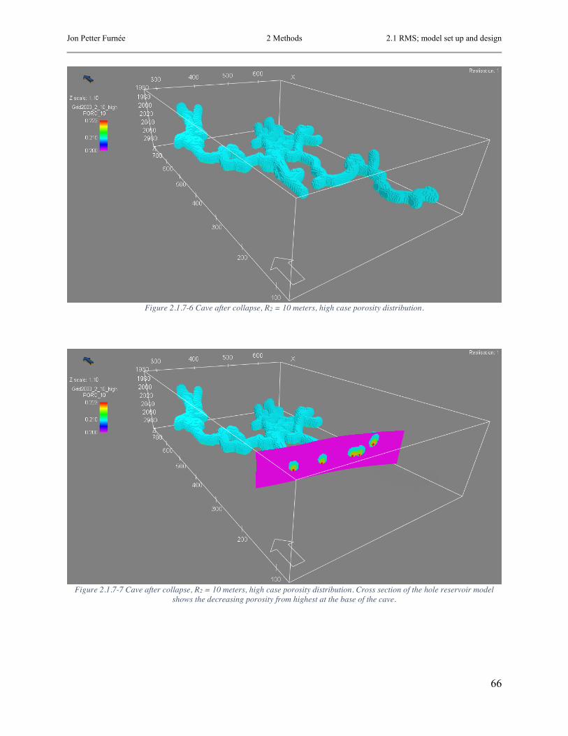
Jon Petter Furnée 2 Methods 2.1 RMS; model set up and design
66
Figure 2.1.7-6 Cave after collapse, R2 = 10 meters, high case porosity distribution.
Figure 2.1.7-7 Cave after collapse, R2 = 10 meters, high case porosity distribution. Cross section of the hole reservoir model
shows the decreasing porosity from highest at the base of the cave.

Jon Petter Furnée 2 Methods 2.1 RMS; model set up and design
67
Figure 2.1.7-8 Cross section of high case porosity distribution with R2 = 10 meters. Notice the decreasing porosity outwards.
Figure 2.1.7-9 Cross section of high case permeability distribution with R2 = 10 meters. Notice the decreasing permeability
outwards.

Jon Petter Furnée 2 Methods 2.1 RMS; model set up and design
68
2.1.8 Fracture model To create a realistic reservoir model of a karst system, fractures have to be accounted for. Large
caves develop in and expand pre-existing fractures (see section 1.3.1). Figure 2.1.8-1 below shows
an image of the cave geometry as seen from above and a rose diagram presenting the main direction
of the cave passages. The cave passage directions and the resulting rose diagram were found by
measuring length and direction of each passage, and use these values to stack up total length for
each measured direction. Then a macro in Excel was used to split up each direction in one meter
segments, and the values were used as input for dip direction in GeoRose 0.4.0, designed by Yong
Technology Inc.
Figure 2.1.8-1 Fracture rose of cave passages. Three main fracture directions are 15, 90, and 170 degrees. Figure from GeoRose 0.4.0, designed by Yong Technology Inc. These are cumulative lengths of measured fracture directions.

Jon Petter Furnée 2 Methods 2.1 RMS; model set up and design
69
This rose diagram suggests three main fracture directions, which are listed in Table 2.1.8-1 below.
These directions are used as input to fracture modeling in RMS. We see that the assumption in
Chapter 2.1.5 to set the grid rotation to an angle of 15 degrees, matches one of the main fracture
directions of the cave system.
Table 2.1.8-1 Input for fracture modeling in RMS.
Fracture name
Orientation [degrees]
Orientation variability
Fracture Thickness [m]
Density [fractures/m]
Length [m]
Length Variability
Frac15 15 5 1 1 50 5 Frac90 90 5 1 1 50 5 Frac170 170 5 1 1 10 1
The rest is set to default RMS values. Table 2.1.8-2 Default RMS values in fracture modeling.
Aperture [µm] 50 Stiffness 0.8 Thickness variability 0 Truncation probability 1
A fracture model is created based on Table 2.1.8-1 and presented in Figure 2.1.8-2.
Figure 2.1.8-2 Screenshot showing modelled fractures in RMS in one grid layer. The fractures are distributed stochastically based on input values from Table 2.1.8-1

Jon Petter Furnée 2 Methods 2.1 RMS; model set up and design
70
The fracture modeling module in RMS facilitates dual-porosity modeling and single-porosity
modeling. Dual-porosity modeling is used to create the fracture porosity based on input from the
fracture model (i.e, fracture length, aperture and orientation). The fracture porosity is added to the
porosity parameter using the calculator in RMS, so that the final porosity parameter is ready for
export in the reservoir model. Single-porosity modeling, however, is used to create permeability
parameters in X and Y direction. Here the fracture permeability is added to the matrix permeability
and two new permeability parameters are created for the X and Y direction respectively. There is,
however, no function to add fracture permeability in the Z-direction, so this remains the same.
This is a shortcoming of the software which will lead to the vertical permeability being
underestimated. This will not be further addressed here as it goes beyond the scope of this thesis.
Figure 2.1.8-3 Cross sections of high case permeability (Y-direction) distribution with R2 = 10 meters including fractures. Notice the decreasing permeability outwards. Compare to Figure 2.1.7-9, the permeability has increased with 46.79 mD.

Jon Petter Furnée 2 Methods 2.1 RMS; model set up and design
71
2.1.9 Upscaling of grid model for fluid flow Geo-models commonly contain a lot of detailed information, not all of this information has bearing
on flow behavior. To save computing time while simulating fluid flow in Eclipse, it is important
to minimize the number of grid cells used while maintaining enough detail to ensure that features
critical to fluid flow are captured. The process of reducing the number of grid cells by merging
them is known as upscaling. A simulation model normally has a coarser grid-resolution than the
geological grid model. It is important to ensure that no information that could influence flow is
lost during upscaling. A number of test runs were carried out on each model to check the
performance of the upscaling.
Roxar (2013b) defines rescaling as the process of assigning values to an Output Grid based on the
values in an Input Grid with different geometry, or in this case the same model volume with a
coarser grid. Typically, an input grid is a result of a geological modeling process, while an output
grid is designed for flow simulation. In general:
x Upscaling - The output grid is coarse, while the input grid has a finer resolution
x Downscaling - The output grid is fine while the input grid is coarse
The output grid should ideally be aligned with the input grid and cover approximately the same
volume. (Roxar, 2013c, Roxar, 2013a).
New Grid models were created (Table 3.1.1-1). They were generated in the same manner as
described above for Grid2000_2. The only difference is that they have 4, 8, 16, and 32 meters grid
cell diameter. A grid cell diameter of 4 meters, results in a 64 m3 grid cell. As the grid cells are
cubes, each side should be equal length. Redefining grid resolution is straightforward, the
challenging part is to recalculate parameter properties for these cells. This is carried out by
Rescaling (Tasks – Flow properties – Rescaling). As input grid model, Grid2000_2 is used. The
main properties to assign to the four new grid models are porosity (1 parameter) and permeability
(3 parameters for X-, Y- and Z-direction. The available rescaling methods for porosity and
permeability in RMS are given in Table 2.1.9-1 below.

Jon Petter Furnée 2 Methods 2.1 RMS; model set up and design
72
Table 2.1.9-1 Available rescaling methods for porosity and permeability in RMS. Green mark on used methods.
Output type Input type Method
Porosity Parameter Arithmetic
Permeability Parameter Diagonal tensor
Arithmetic
Geometric
Harmonic
Power
Arithmetic-Harmonic
Harmonic-Arithmetic
Full tensor
Well permeability
For porosity, the choice of rescaling method is easy. The arithmetic method is used.
For permeability, there are several methods available, and the choice of method can affect the
results. For this case, the diagonal tensor method is sufficient, and has been chosen. Full tensor
method would be the best, but Eclipse cannot handle a total of six directional permeability’s.
Problems with rescaling can occur in the transition between the high permeability in the collapsed
cave, and the lower permeability outside the cave. This because the averaging of cell parameters
in these cases become challenging. This will not be further addressed as it goes beyond the scope
of this thesis.
Arithmetic mean averages all of the grid squares in the fine grid into the new square.
Diagonal tensor method solves a pressure system for each cell with certain boundary conditions.
A detailed evaluation of the upscaling methods implemented in RMS is outside the scope for this
thesis. For theory behind these methods, see the Roxar (2013a, 2013b) user manual.

Jon Petter Furnée 2 Methods 2.1 RMS; model set up and design
73
Figure 2.1.9-1 Rescaling from GRID2000_2_12_high to GRID2000_4_12_high. From the names it follows that high case including collapsed cave with radius 12 meter is upscaled from grid cell diameter 2 to 4 meters. It follows that 8 grid cells in the
finer grid becomes one in the coarser grid. See Appendix Chapter 7.1.1 for grid model names.

Jon Petter Furnée 2 Methods 2.1 RMS; model set up and design
74
2.1.10 Export of grid (RMS) model to simulation model (Eclipse) A total of 26 grid models (see list Table 3.1.1-1) were exported as Eclipse simulation models.
Figure 2.1.7-1 shows the eight cases for grid cell dimension 2m × 2m × 2m. Identical sets of 8
cases where produced using cell dimensions of 4m × 4m × 4m and 8m × 8m × 8m. Two
additional low-resolution cases for “low case” (i.e. host rock porosity of 5 %) with a collapsed
radius 10 meters were generated, having grid cell dimension of 16m × 16m × 16m and 32m ×
32m × 32m respectively. Names of grid and simulation models are explained in Appendix 7.1.1
and 7.1.2. Figure 2.1.10-1 shows how simulation models are exported from RMS, and which
petrophysical parameters are included. The simulation model uses porosity- and permeability (in
three directions) including fractures as described in Chapter 2.1.8.
Figure 2.1.10-1 how simulation models are exported in RMS, and which petrophysical parameters are included. The simulation
model uses porosity- and permeability (in three directions) including fractures as described in Chapter 2.1.8.

Jon Petter Furnée 2 Methods 2.2 Eclipse; simulation of fluid flow
75
2.2 Eclipse; simulation of fluid flow
2.2.1 Introduction to Eclipse The RMS models were exported as Eclipse flow simulation models. Some of the default values
from the exported simulation settings were changed and are discussed in the following sub-
chapters. A complete .data-file, Lowcase_cave_rc10.data, is attached in the Appendix Chapter 7.3
as an example. The names of the .data-files are largely self-explanatory: First it states whether the
model is high- or low case with respect to porosity, secondly whether it includes a cave (else
nocave). If the model includes a cave, the radius after collapse is defined (here 10 meters, as it
follows from the name rc10). Throughout this thesis, 40 different cases have simulated with respect
to high- and low case, cave radiuses, upscaling, and increased maximum injection rate (see Table
3.1.1-1. Although the .data-file was exported as a fluid simulation model from RMS, it is modified
quite a bit to obtain the best result and layout, as outlined below.
2.2.2 RUNSPEC section The RUNSPEC section defines run specifications. It includes a description of the run, such as grid
size, table sizes, number of wells, which phases to include and so forth. The title of the .data-file
was changed to Lowcase_cave_rc10 the name of the .data-file. Start date was set to 01. January
2014, and the system was defined as a dead oil system (only oil and water).
The linear solver stack size, NSTACK, was set to the value 100 (equal to LITMAX, which
specifies the maximum number of linear iterations in a Newton iteration). NSTACK is set equal
to LITMAX if enough memory on computer. NUPCOL was raised to 10, as a result of a warning
while simulating that the value should be raised from 3.
2.2.3 GRID section The GRID section defines the grid dimensions and shape, including petrophysics (porosity,
permeability, net-to-gross etc.). This was all kept default from the export .data-file from RMS.

Jon Petter Furnée 2 Methods 2.2 Eclipse; simulation of fluid flow
76
2.2.4 PROPS section The PROPS section defines fluid and rock properties such as relative permeability, PVT data, rock
compressibility, surface density and dissolved gas concentration. Values are defined in the .data-
file in the appendix. These values are kept constant in all simulation cases. Below, two figures
showing the relative permeability curves for oil and water, and PVT data for dead oil are presented.
The data presented in the curves are derived from a semester assignment (exam) in the Reservoir
Simulation course (MAT255), at the University of Bergen spring semester 2013.
Figure 2.2.4-1 Relative permeability curves for oil (Kro) and water (Krw)
Figure 2.2.4-2 PVT-data for dead oil. Bo – Volume formation factor for oil, ViscO – Oil viscosity.
0
0,2
0,4
0,6
0,8
1
0 0,2 0,4 0,6 0,8 1
Relp
erm
Sw
Relative permeability curves Oil&Water
Krw
Kro
11,05
1,11,15
1,21,25
1,3
200,00 250,00 300,00 350,00 400,00
Pressure (bar)
PVT-data for dead oil
Bo
ViscO

Jon Petter Furnée 2 Methods 2.2 Eclipse; simulation of fluid flow
77
2.2.5 REGIONS section The REGIONS section is used to give user defined report regions. All is kept default from the
exported .data-file from RMS, there is only one region.
2.2.6 SOLUTION section The SOLUTION section gives the models equilibration data e.g. a description of how the model
is to be initialized. “The EQUIL keyword sets the contacts and pressures for conventional
hydrostatic equilibrium” (Schlumberger, 2013). The oil-water contact is defined below the
reservoir to get a completely oil-filled reservoir with no mobile water present. The gas-oil contact
is defined above the reservoir to avoid including gas in model.
2.2.7 SUMMARY section This section is used to define simulation output by specifying which data items to write to report
files.
2.2.8 SCHEDULE section The SCHEDULE section specifies the operations to be simulated in Eclipse. This includes
production and injection controls and constraints, and the times at which output reports are
required (Schlumberger, 2013). See SCHEDULE section in .data-file in Appendix, Chapter 7.3,
for the setup. The setup is the same for all simulation cases, with minor changes such as well
placement (fewer grid cells as grid cell diameter increases) for upscaled models, and production
and injection rates for high- and low case. To be able to compare the different simulations,
production and injection rates are kept constant within the high- and low cases.
Wells are defined, as well as tuning parameters and time control. Table 7.1.5-1 in Appendix 7.1.5
summarizes the placement of wells WP1 (Well Producer 1), WI1 and WI2 (Well Injector 1 and 2)
in all models. Varying grid cell size leads to different cell numbers were the wells are completed.
Visual inspection ensures that the wells are completed at the same location for all cases.

Jon Petter Furnée 2 Methods 2.2 Eclipse; simulation of fluid flow
78
Figure 2.2.8-1 Visual inspection of grid cells that give approximately the same well placement in the different upscaled grid models. The original well placement in the grid with cell diameter of 2 meters is used as base for the other grids.
Figure 2.2.8-2 Well placement original (not upscaled) model. Grid diameter 2 meter. WP1 (Well Producer 1), WI1 and WI2 (Well Injector 1 and 2)
Figure 2.2.8-3 Well placement upscaled model. Grid diameter 4 meter. WP1 (Well Producer 1), WI1 and WI2 (Well Injector 1 and 2)
Grid diameter 2 meter
Grid diameter 4 meter
Grid diameter upscaled model: 8 meter
Grid diameter upscaled model: 4 meter

Jon Petter Furnée 2 Methods 2.2 Eclipse; simulation of fluid flow
79
Figure 2.2.8-4 Well placement upscaled model. Grid diameter 8 meter. WP1 (Well Producer 1), WI1 and WI2 (Well Injector 1 and 2)
Figure 2.2.8-5 Well placement upscaled model. Grid diameter 16 meter. WP1 (Well Producer 1), WI1 and WI2 (Well Injector 1 and 2)
Figure 2.2.8-6 Well placement upscaled model. Grid diameter 32 meter. WP1 (Well Producer 1), WI1 and WI2 (Well Injector 1 and 2)
Grid diameter 8 meter
Grid diameter 16 meter
Grid diameter 32 meter

Jon Petter Furnée 2 Methods 2.2 Eclipse; simulation of fluid flow
80
The production rates are defined (using WCONPROD keyword) based on complete drainage of
the reservoir in 10 years. For high case the volume of oil in place is approximately 1387000 Sm3.
Production distributed over 10 years gives a daily production of 380 Sm3/day. For low case, the
production was set to 100 Sm3 based on the same calculation with a lower oil volume. Total
maximum injection rate (spread equal on the two injection wells) for high- and low case is set to
400 Sm3 and 100 Sm3 respectively (with WCONINJE keyword).
It is however not expected that the reservoir can produce all of the oil in place. The pressure loss
and water production will ensure that production rates will eventually fall. The list of report dates
were set with the DATES keyword. It was set write report files every 1st of the month, with the
first report date set to 1. Feb 2014 and the last to 1. Jan 2029. This gives a simulation run for 15
years.
The TUNING keyword was set to default on all values except those presented in Table 2.2.8-1. Table 2.2.8-1 Values not defaulted in TUNING keyword in SHEDULE section
Parameter Description of parameter Value
TSINIT Maximum length of next time step 0.1
TSMAXZ Maximum length of time steps after the next 5
TSMINZ Minimum length of all time steps 0.1
NEWTMX Maximum number of Newton iterations in a time step 40
NEWTMN Minimum number of Newton iterations in a time step 1
LITMAX Maximum number of linear iterations in a Newton iteration 100
LITMIN Minimum number of linear iterations in a Newton iteration 1
LITMAX was set to the same value as NSTACK in the RUNSPEC section. Other changes were
made because of the number of warnings that appeared during simulation, telling to increase
certain values. LITMAX specifies the maximum number of linear iterations in a Newton iteration.
To avoid the calculations to run circles, a high enough NSTACK has to be set. Usual these two are
set equal.
The keyword GCONINJE (Group Control Injection) was included to try to reduce pressure loss in
reservoir under production. The record VREP under GCONINJE keyword ensures that the pressure

Jon Petter Furnée 2 Methods 2.2 Eclipse; simulation of fluid flow
81
is stable, by increasing or decreasing water injection. The purpose of including this, is to match
the total reservoir volume injection rate of the field with its production voidage rate. The specified
water injection rate under WCONINJE keyword, is the maximum injection rate, this means that if
the production voidage rate demands another injection rate to maintain the reservoir pressure it
will adjust automatically. If however, maximum injection rate is set to low, this will not be
possible.
The data-file was ended with the END keyword.

Jon Petter Furnée 3 Results and discussion 3.1 Results and discussion
82
3 Results and discussion 3.1 Results and discussion This thesis presents a workflow for modeling paleokarst reservoirs in RMS using information
about the geometry of a pre-existing cave system as a starting point. Furthermore, an attempt is
made to investigate how fluid flow will be affected by changing certain model parameters. The
effect of changing the radius of the collapse is investigated and the impact of upscaling the
reservoir model is studied. Finally, some simulation results are presented to illustrate fluid flow
behavior in this reservoir model. The results can be used by the industry to compare with real time
production curves from karst reservoirs. The publicly available data on this type of research is
limited and therefore simulation results can at present not be compared to any similar previous
work or examples.
3.1.1 The paleokarst reservoir model One of the main results of the present study is a workflow for building reservoir models
representing a real case geometry of a collapsed cave system. The method provides the basic
concepts for building reservoir models using any conceivable cave geometry as a starting point.
In other words, if a skeleton line of a cave geometry is provided (based on any real- or synthetic
data), it will be possible to recreate this geometry in RMS as parts of a reservoir model.
To sum up the methods chapter (see Figure 3.1.1-1, numbers (x) in the text indicates the marks in
the figure), a survey point dataset from Setergrotta cave is used to create a skeleton line of the cave
geometry (1). Further, the stratigraphic framework was created and the horizons were mapped (2).
These mapped horizons were used to create a structural model and horizon model (3), which were
essential for creating a grid (4). The grid consists of 1323735 grid cells with diameter 2 meters.
Total reservoir volume equals 1323735 × 2 × 2 × 2 m3 ≈ 10.6 MSm3. Further, geometric
modeling (5) defines the radial distance from the refined points of the skeleton line, and is used to
create the original cave geometry with radius 5 meters (6). Another seven geometric models are
created to be able to assign petrophysical values and recreate the decreasing porosity and
permeability trend from cave bottom to the collapsed cave roof (7). After assigning petrophysical
values to the models (8), fractures (9) are introduced. These fractures increase the porosity and
permeability of the reservoir model. The final model (10) includes fractures.

Jon Petter Furnée 3 Results and discussion 3.1 Results and discussion
83
Figure 3.1.1-1 Figure that sums up building the models in RMS. (1) measure points/skeleton line, (2) stratigraphic framework/horizon modeling, (3) structural model/horizon model, (4) grid model, (5) geometric model, (6) cave with radius R1 = 10 meters, (7) assigning petrophysical properties with different geometric models, (8) petrophysical properties, (9) fracture rose,
(10) final model with fractures.

Jon Petter Furnée 3 Results and discussion 3.1 Results and discussion
84
Finally, the eight cases described in Figure 2.1.7-1 were upscaled to grid cell dimensions of 4, 8,
16, and 32 meters to run test on the effects of upscaling. All reservoir models listed in Table 3.1.1-1
were exported as Eclipse simulation models, and simulated with the production- and maximum
injection rates specified, as well as well placement described in Figure 2.2.8-2, Figure 2.2.8-3,
Figure 2.2.8-4, Figure 2.2.8-5, Figure 2.2.8-6, and Table 7.1.5-1. The maximum injection rate had
to be increased for some of the simulations to maintain the reservoir pressure with the GCONINJE-
keyword, as described in Chapter 2.2.8.
The suite of “high case” paleokarst reservoir model refers to a background/host rock porosity of
20%, while “low case” refers to models with a background/host rock porosity of 5 % (see Chapter
2.1.7). If a collapsed cave is present, porosity and permeability values are higher within the radius
of the collapsed cave, than in the background. For the models used here, the collapsed cave radius
(R2) was set at 10, 12 and 14 meters. Grid cells used here are cubes, and grid cell dimension is 2
meters for the original reservoir model, while the upscaled models have a grid cell diameter of 4,
8, 16, and 32 meters. In Chapter 2.2.8, it is mentioned that it is desirable to maintain the pressure
within the reservoir. Hence, the GCONINJE-keyword defines the maximum injection rate, and
had to be set higher for some simulations (see Table 3.1.1-1). Consequently, a distinction between
a low- and high maximum injection rate for low case (100 and 200 Sm3/day respectively) and high
case (400 and 800 Sm3/day respectively) has been made.

Jon Petter Furnée 3 Results and discussion 3.1 Results and discussion
85
Table 3.1.1-1 A total of 40 simulations were carried out throughout this thesis. 26 different cases (blue color) with respect to high- and low case, geometry, and upscaled versions. In addition to this 14 re-simulations (green color) were carried out with injection rates doubled (we will come back to why in Chapter 3.1.4).
Grid cell Diameter [m]
High/Low case
Radius collapsed cave [m]
Production rate [Sm3/day]
Max Injection rate [Sm3/day]
2 High No cave 380 400 2 High 10 380 400 2 High 12 380 400 2 High 14 380 400 4 High No cave 380 400 4 High 10 380 400 4 High 12 380 400 4 High 14 380 400 8 High No cave 380 400 8 High 10 380 400 8 High 12 380 400 8 High 14 380 400 2 Low No cave 100 100 2 Low 10 100 100 2 Low 12 100 100 2 Low 14 100 100 4 Low No cave 100 100 4 Low 10 100 100 4 Low 12 100 100 4 Low 14 100 100 8 Low No cave 100 100 8 Low 10 100 100 8 Low 12 100 100 8 Low 14 100 100 16 Low 10 100 100 32 Low 10 100 100 2 High No cave 380 800 2 High 10 380 800 2 Low No cave 100 200 2 Low 10 100 200 4 High No cave 380 800 4 High 10 380 800 4 Low No cave 100 200 4 Low 10 100 200 8 High No cave 380 800 8 High 10 380 800 8 Low No cave 100 200 8 Low 10 100 200 16 Low No cave 100 200 32 Low 10 100 200
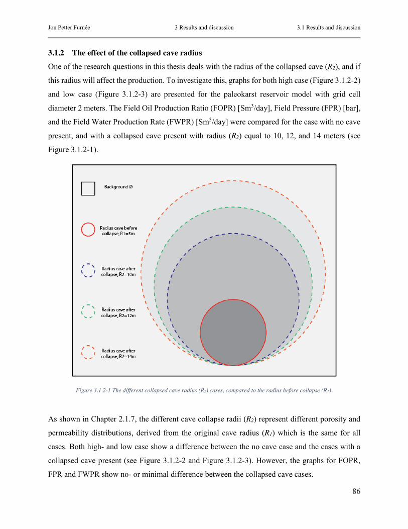
Jon Petter Furnée 3 Results and discussion 3.1 Results and discussion
86
3.1.2 The effect of the collapsed cave radius One of the research questions in this thesis deals with the radius of the collapsed cave (R2), and if
this radius will affect the production. To investigate this, graphs for both high case (Figure 3.1.2-2)
and low case (Figure 3.1.2-3) are presented for the paleokarst reservoir model with grid cell
diameter 2 meters. The Field Oil Production Ratio (FOPR) [Sm3/day], Field Pressure (FPR) [bar],
and the Field Water Production Rate (FWPR) [Sm3/day] were compared for the case with no cave
present, and with a collapsed cave present with radius (R2) equal to 10, 12, and 14 meters (see
Figure 3.1.2-1).
Figure 3.1.2-1 The different collapsed cave radius (R2) cases, compared to the radius before collapse (R1).
As shown in Chapter 2.1.7, the different cave collapse radii (R2) represent different porosity and
permeability distributions, derived from the original cave radius (R1) which is the same for all
cases. Both high- and low case show a difference between the no cave case and the cases with a
collapsed cave present (see Figure 3.1.2-2 and Figure 3.1.2-3). However, the graphs for FOPR,
FPR and FWPR show no- or minimal difference between the collapsed cave cases.

Jon Petter Furnée 3 Results and discussion 3.1 Results and discussion
87
Figure 3.1.2-2 High case with low injection rate. Test of the effect of the radius of the collapsed cave (R2).
Figure 3.1.2-3 Low case with low injection rate. Test of the effect of the radius of the collapsed cave (R2).

Jon Petter Furnée 3 Results and discussion 3.1 Results and discussion
88
It appears that the different collapse radius (R2) cases tested in this thesis yield the same production
results. When introducing a void volume (original cave volume with radius (R1) equal 5 meters)
to the background, the increase in porosity and permeability added to the background when the
cave collapses, will be constant, no matter how big the radius collapse would be. The increase in
volume is derived directly from the volume of the original cave geometry and is a constant volume
added to the background in all cases.
If the original cave volume had been spread evenly and homogenized the background on an infinite
volume, the increase would most likely not be noticed at all. However, since the increase of radius
goes from 5 meters (R1) to 10, 12, or 14 meters (R2), the production curves will notice the
difference from the no-cave example, but not the difference between the radius increases. Within
the scope of test performed in this thesis, no effect is shown from the increase of collapse radius
from 10 to 12 or 14 meters. The drainage volume and pore volume remains the same, but the
distribution of the volume within these cases, will not matter for the production curves. Figure
3.1.2-4 sums up the observations of the radius (R2) cases, and concludes that there is no difference
between the collapsed cave radii. Therefore, the green boxes highlights which cases should be
targeted for further research, whereas further work on the red cases has less priority.
Figure 3.1.2-4 This figure is an continuation of Figure 2.1.7-1 and sums up the observations done when it comes to the radius of the collapsed cave (R2). It shows that there is no difference between the collapsed cave radiuses, and the green boxes represent
the cases for further research, while the red boxes are dropped cases.

Jon Petter Furnée 3 Results and discussion 3.1 Results and discussion
89
As presented above, there is no difference between the production curves in the paleokarst
reservoir models including three different collapsed cave radius cases (R2). It follows that if the
radius before collapse (R1) is constant within the boundaries of this thesis, the increase in porosity
and permeability is constant and added to the background in all cases, and will result in the same
simulation results. However, if cave radius (R1) would be larger, more pore space could potentially
be added to the background, and production curves would presumably look different.
For further simulation comparison, it will be sufficient to compare the “no cave” case with one of
the collapsed cave cases. For simplicity, the paleokarst reservoir model will include a collapsed
cave with radius (R2) equal to 10 meters as Figure 3.1.2-4 illustrates.

Jon Petter Furnée 3 Results and discussion 3.1 Results and discussion
90
3.1.3 Upscaling of paleokarst reservoir models As discussed in Chapter 2.1.9 it is desirable to upscale the reservoir grid model to reduce
simulation time. However, the coarsened grid may lose vital information about the reservoir
petrophysical properties when merging cells. As an example, eight grid cells in the reservoir model
with grid cell dimension 2m × 2m × 2m meters and different parameter values are averaged into
one grid cell in the 4 meter grid cell diameter cases. Furthermore, 64, 512 and 4096 grid cells with
diameter 2 meters are needed to create one single grid cell in the 8, 16 and 32 meter grid cell
diameter cases, respectively. As follows, it is vital that upscaling is well tested before potentially
running the rest of the simulations on a coarser grid. Figure 3.1.3-1 shows how the paleokarst
reservoir grid model looks on different scales. Visually, much of the collapsed cave structure is
still captured at an 8 meter scale. For the 16 and 32 meter scale however, the petrophysical
properties are smoothened on a too large scale in order to be able to detect the cave geometry.
Figure 3.1.3-1 The figure illustrates how the paleokarst reservoir grid model looks on different scales. Upscaled models have a grid cell diameter of 4,8,16,and 32 meters. Here the porosity distribution for low case with fractures is shown, with a collapsed
cave with radius R2 present.
It becomes obvious that there is a constraint with respect to well placement in the coarser grids, as
in the finer grid cells, the wells are placed within the collapsed cave structure, whereas in the coarse
models the target becomes less easy to define. The upscaled models should ideally have been
upscaled as a power of three; it would then always be possible to set a well in the center point. For
the completion depth as well, problems occur, especially for the 32 meter grid cell diameter case.
Here there are only two layers to choose between when it comes to well placement and completion.

Jon Petter Furnée 3 Results and discussion 3.1 Results and discussion
91
Figure 3.1.3-2 All curves represent the Field Oil Production Rate (FOPR) for all upscaled cases with a low injection rate. All production curves are simulations from the same case; low case with a collapsed cave radius (R2) equal to 10 meters.
Figure 3.1.3-2 above represents the Field Oil Production Rate (FOPR) for all upscaled cases with
low injection rate. All of the production curves are simulations derived from the same case; low
case with a collapsed cave radius (R2) equal to 10 meters. It seems that the production curves more
or less are similar for grid cell diameter up to 16 meters. However, the 32 meter grid cell diameter
case deviates from the other curves.
Figure 3.1.3-3 below represent the same graph as Figure 3.1.3-2 above. The difference between
the two cases however, is that the increased maximum injection rate is doubled. As a result, the
FOPR-curves in Figure 3.1.3-3 differ from the ones in Figure 3.1.3-2, but the same observation is
made, the 32 meter grid cell diameter case deviates from the other curves.

Jon Petter Furnée 3 Results and discussion 3.1 Results and discussion
92
Figure 3.1.3-3 All curves represent the Field Oil Production Rate (FOPR) for all upscaled cases with a high injection rate. All production curves are simulations from the same case; low case with a collapsed cave radius (R2) equal to 10 meters.
It seems that if the grid cell diameter exceeds the diameter for the collapsed cave diameter (R2 =
10 meters, so the diameter = 2 × 10 = 20 meters), the production curves will start to deviate.
Even though the paleokarst reservoir model with grid cell diameter of 32 meters deviates from the
other cases, it still represents a quite good representation of the oil production. It should however
be emphasized that the well placing becomes more difficult for the coarser grid models, and it will
be impossible to set the Z-axis well interval to be equal for the 32 and 2 meter grid cell diameter
cases. This will have effects on the production curves.
Ø. Pettersen (2015, pers. comm., 14 April) mentioned that the difference between the production
curves (up to 16 meter grid cell diameter), could be caused by weight effect of the fluids. The
larger grid cells could result in a different flow pattern in Eclipse.
Figure 3.1.3-4 illustrates the time usages in seconds for the simulation of the different upscaled
paleokarst reservoir models. The X-axis represents the grid cell diameter in meters, while the Y-
axis shows the simulation duration in seconds. The practical utility of upscaling becomes very
evident. By increasing the grid cell dimension from 2 meters to 4 meters, simulation time falls

Jon Petter Furnée 3 Results and discussion 3.1 Results and discussion
93
from 18600 seconds (more than 5 hours) to 730 seconds (approximately 12 minutes). In other
words, by increasing the grid cell dimension eight times, the time usage cut by 96%. The grid cell
diameter of 8 meters uses 64 seconds, while the 16 and 32 meter cases uses 20 and 17 seconds
respectively.
Figure 3.1.3-4 Time usages in seconds for the simulation of the different upscaled models. The x-axis represent the grid cell diameter in meters, while the y-axis shows the simulation time in seconds.

Jon Petter Furnée 3 Results and discussion 3.1 Results and discussion
94
3.1.4 Production curves in paleokarst reservoirs Graphs for Field Oil Efficiency (FOE) (see equation 10), Field Pressure (FPR) [bar], Field Oil
Production Rate (FOPR) [Sm3/day], Field Water Production Rate (FWPR) [Sm3/day], Field Water
Injection Rate (FWIR) [Sm3/day], and Field Water Cut (FWCT) (see equation 11) are presented
and compared for the following cases (Figure 3.1.4-1).
Figure 3.1.4-1 This figure gives an overview over the different cases where production curves are compared
𝐹𝑂𝐸 = Oil in placeinitial−Oil in placepresent
Oil in placeinitial (10)
𝐹𝑊𝐶𝑇 = Produced waterTotal liquids produced
(11)
A complete list of symbols is presented in Appendix 7.1.4. Below, the graphs for high- and low
case with low injection rate (Figure 3.1.4-2 and Figure 3.1.4-3) are compared.
8 casesGrid cell diameter 2 meters
High case (Background Ø = 20%)
Collapsed caveR2 = 10 meters
Low max. injection rate400 Sm3/day
High max. injection rate800 Sm3/day
No cave
Low max. injection rate400 Sm3/day
High max. injection rate800 Sm3/day
Low case (Background Ø = 5%)
Collapsed caveR2 = 10 meters
Low max. injection rate100 Sm3/day
High max. injection rate200 Sm3/day
No cave
Low max. injection rate100 Sm3/day
High max. injection rate200 Sm3/day

Jon Petter Furnée 3 Results and discussion 3.1 Results and discussion
95
Figure 3.1.4-2 This graph presents the FOE, FOPR, FPR, FWPR, and FWIR for high case with low injection rate.
Figure 3.1.4-3 This graph presents the FOE, FOPR, FPR, FWPR, and FWIR for low case with low injection rate.
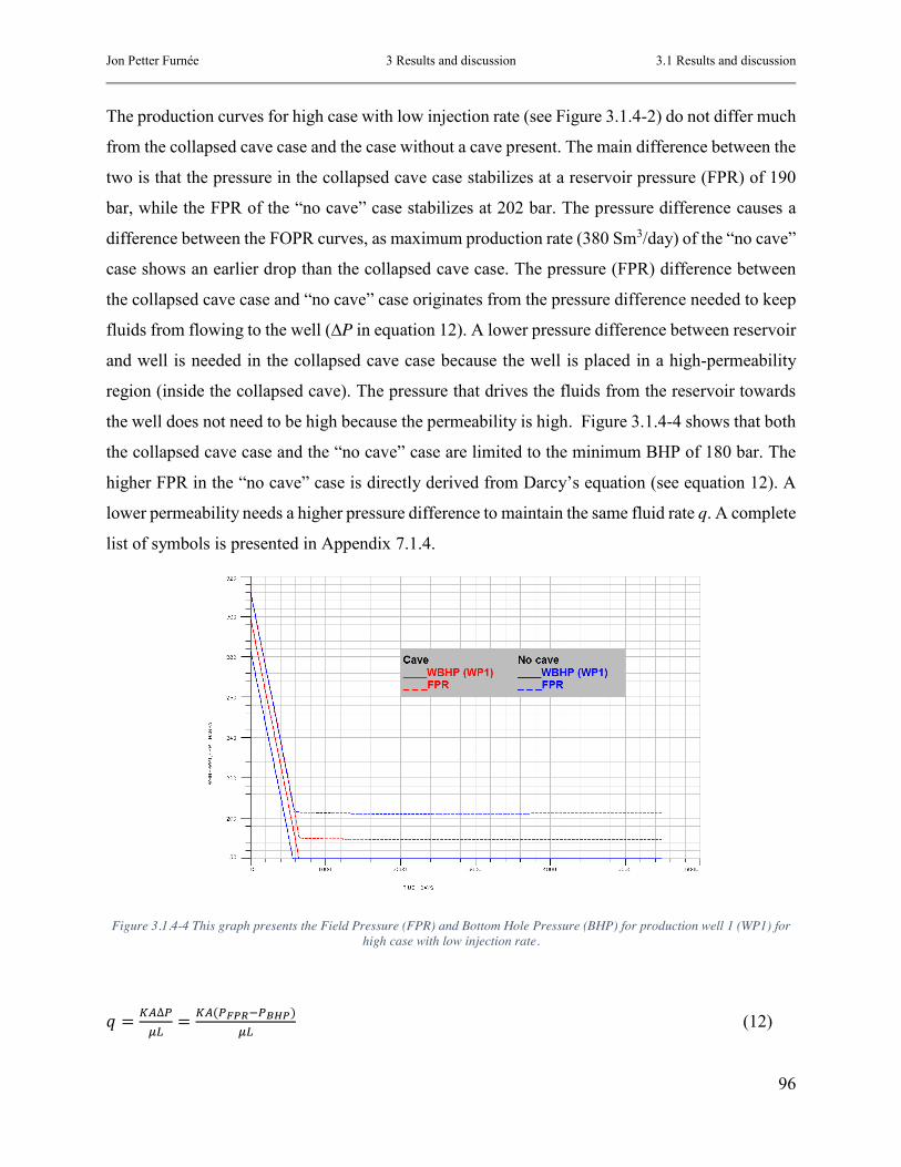
Jon Petter Furnée 3 Results and discussion 3.1 Results and discussion
96
The production curves for high case with low injection rate (see Figure 3.1.4-2) do not differ much
from the collapsed cave case and the case without a cave present. The main difference between the
two is that the pressure in the collapsed cave case stabilizes at a reservoir pressure (FPR) of 190
bar, while the FPR of the “no cave” case stabilizes at 202 bar. The pressure difference causes a
difference between the FOPR curves, as maximum production rate (380 Sm3/day) of the “no cave”
case shows an earlier drop than the collapsed cave case. The pressure (FPR) difference between
the collapsed cave case and “no cave” case originates from the pressure difference needed to keep
fluids from flowing to the well (∆P in equation 12). A lower pressure difference between reservoir
and well is needed in the collapsed cave case because the well is placed in a high-permeability
region (inside the collapsed cave). The pressure that drives the fluids from the reservoir towards
the well does not need to be high because the permeability is high. Figure 3.1.4-4 shows that both
the collapsed cave case and the “no cave” case are limited to the minimum BHP of 180 bar. The
higher FPR in the “no cave” case is directly derived from Darcy’s equation (see equation 12). A
lower permeability needs a higher pressure difference to maintain the same fluid rate q. A complete
list of symbols is presented in Appendix 7.1.4.
Figure 3.1.4-4 This graph presents the Field Pressure (FPR) and Bottom Hole Pressure (BHP) for production well 1 (WP1) for high case with low injection rate.
𝑞 = 𝐾𝐴∆𝑃𝜇𝐿
= 𝐾𝐴(𝑃𝐹𝑃𝑅−𝑃𝐵𝐻𝑃)𝜇𝐿
(12)

Jon Petter Furnée 3 Results and discussion 3.1 Results and discussion
97
The production curves for low case with low injection rate (see Figure 3.1.4-3) show a difference
between the collapsed cave and the “no cave” case. When the permeability is low, the contrast
between the high permeability inside of the cave and the low permeability in the background/host
rock, is clearly reflected in the graphs. The ”no cave” case cannot produce with the same rates as
the collapsed cave case, simply because flow properties are poor. As Figure 3.1.4-5 illustrates, the
low case without a collapsed cave present is limited to by the Well Bottom Hole Pressure (WBHP)
from the start of production. This limits oil production and therefore the field oil efficiency. The
field pressure (FPR) however does not fall much because of the low production rate.
Figure 3.1.4-5 This graph presents the Field Pressure (FPR) and Bottom Hole Pressure (BHP) for production well 1 (WP1) for low case with low injection rate.
The following graphs (Figure 3.1.4-6 and Figure 3.1.4-7) show production curves for high- and
low case with a high injection rate. The maximum injection rate is doubled from the previous
cases, to keep reservoir pressure relatively stable.

Jon Petter Furnée 3 Results and discussion 3.1 Results and discussion
98
Figure 3.1.4-6 This graph presents the FOE, FOPR, FPR, FWPR, and FWIR for high case with high injection rate.
Figure 3.1.4-7 This graph presents the FOE, FOPR, FPR, FWPR, and FWIR for low case with high injection rate.

Jon Petter Furnée 3 Results and discussion 3.1 Results and discussion
99
The reservoir pressure (FPR) is more or less constant for all cases apart from the low case with
high maximum injection rate including a collapsed cave. This case is limited by the maximum
injection rate, the graph (Figure 3.1.4-7) shows that after approximately 2200 days the FPR drops
simultaneously as the FWIR peaks as 200 Sm3/day. As for the FOPR, it is able to produce with a
constant rate for all cases in the beginning, and decreasing when it is no longer possible to maintain
the initial oil production rate.
Below, Table 3.1.4-1, shows a summary for time to water breakthrough (WBT) as well as Field
Oil Efficiency (FOE) for the eight cases in Figure 3.1.4-1.
Table 3.1.4-1 The table shows time to Water Break Through (WBT) as well as Field Oil Efficiency (FOE) for the eight cases in Figure 3.1.4-1. (H.inj) is written after the cases with high maximum water injection.
High/Low case
Radius collapsed cave
Time to WBT (days)
FOE 5 years (1825 days)
FOE 10 years (3650 days)
FOE 15 years (5475 days)
High No cave 1820 0.445 0.683 0.758 High 10 1820 0.444 0.670 0.747 Low No cave no WBT 0.108 0.216 0.322 Low 10 1900 0.413 0.627 0.693 High (H.inj) No cave 1570 0.500 0.751 0.789 High (H.inj) 10 1550 0.497 0.743 0.786 Low (H.inj) No cave no WBT 0.108 0.216 0.322 Low (H.inj) 10 1445 0.489 0.736 0.771
From Table 3.1.4-1, it is clear that a higher injection rate will increase the field oil efficiency
(FOE). The high case without a collapsed cave has a 3% higher FOE when the water injection rate
is raised. While the high case with a collapsed cave has a 4% higher FOE when the water injection
rate is raised. Furthermore, the low case with a collapsed cave has an 8% higher FOE when the
water injection rate is raised, while the “no cave” case for low case has no change. This because
the water injection is not raised as a result of the poor characteristics of this reservoir.
Figure 3.1.4-8 below presents a summary of FOPR, FWPR, and FWIR for high and low case with
high injection rate.

Jon Petter Furnée 3 Results and discussion 3.1 Results and discussion
100
Figure 3.1.4-8 This graph presents the summary of FOPR, FWPR, and FWIR for high and low case with high injection rate.
It becomes obvious that for the high case, that the porosity and permeability increase introduced
by adding a collapsed cave is not very noticeable. If the reservoir properties already are good, the
improvement is not necessary to be able to produce the field. For low case however, the field oil
efficiency (FOE) is raised from 33.2% to 77.1%, which means that the presence of a collapsed
cave will more than double the FOE for the low case.
One consequence of setting a higher maximum injection rate is an increase in water production.
See Figure 3.1.4-9 below for the water cut.
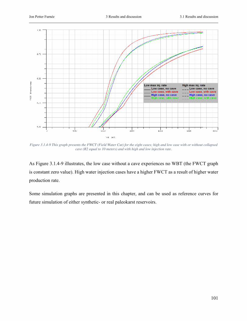
Jon Petter Furnée 3 Results and discussion 3.1 Results and discussion
101
Figure 3.1.4-9 This graph presents the FWCT (Field Water Cut) for the eight cases; high and low case with or without collapsed cave (R2 equal to 10 meters) and with high and low injection rate.
As Figure 3.1.4-9 illustrates, the low case without a cave experiences no WBT (the FWCT graph
is constant zero value). High water injection cases have a higher FWCT as a result of higher water
production rate.
Some simulation graphs are presented in this chapter, and can be used as reference curves for
future simulation of either synthetic- or real paleokarst reservoirs.

Jon Petter Furnée 4 Conclusions
102
4 Conclusions The thesis present a procedure for modeling paleokarst reservoirs in RMS. The workflow can be
used for modeling paleokarst reservoir configurations deriving from any conceivable cave
geometry. Paleocave systems of any imaginable geometry, as long as a skeleton line that represent
this geometry is created.
Furthermore, the effect of the radius of the cave after collapse (R2) is tested by comparing
production curves derived from simulation of fluid flow in the paleokarst reservoir with Eclipse.
The research shows that within the scope of tests carried out in this thesis, changing the collapse
radiuses (R2 equal to 10, 12 or 14 meters) will not affect the simulation results. As long as the
volume of the cave before collapse is constant (as R1 is constant equal to 5 meters), the increase of
porosity (and thereby permeability) added to the background in each collapsed cave radius case is
constant. In practice, this implies that the initial dimensions of the cave system appear to be
relatively more important than how far the collapse of the cavity extends into the surrounding
formation.
The main conclusion with respect to upscaling test performed here, is that a grid cell dimension of
4 or 8 meters provides a sufficiently detailed approximation of an the original reservoir model with
2 meters grid cell diameter. The simulated production curves indicate that results start to deviate
from the initial fine-scale model when the grid cell dimension of the upscaled model exceed the
collapsed cave diameter. For later studies, a grid cell diameter of 4 or 8 meters (for a reservoir
model of the same size) is recommended. The amount of CPU time saved is substantial, which for
practical purposes implies that more models and simulations can be performed in a shorter time.
Finally, this thesis presents several simulation result that can be used as reference curves for future
simulation of either synthetic- or real paleokarst reservoirs.

Jon Petter Furnée 5 Future work and limitations with this study
103
5 Future work and limitations with this study Future work within modeling and simulation of fluid flow in paleokarst reservoirs should focus on
creating a set of realistic models, to create a “multiple case atlas” which can be used as a guideline
for exploration and production of this type of reservoirs. Additional realistic models, brings the
possibility to choose the best representation of the real case reservoir oil companies are working
with. If the conditions governing karst morphology in a given reservoir formation can be
constrained (e.g. climate, lithology, tectonics, sea-level change), this can be used to make
assumptions about shape orientation and dimensions of karst forms including cave systems. Using
the methods outlined in this thesis, a number of plausible reservoir models can be constructed and
tested to add exploration and production work in these formations.
Better studies of outcrops and access to well data of paleokarst could contribute to reservoir models
with better representing petrophysical properties, and thereby improve the models further.
Another interesting aspect opened up by this study, is that it offers the potential to carry out seismic
forward modeling of paleokarst reservoir models. Comparison of seismic signatures from
systematically generated paleokarst reservoir models with real-life seismic from known or
suspected paleokarst reservoirs, could significantly enhance our ability to provide for optimized
production from these complex features. The recognition of paleocave systems in seismic, could
be vital information when it comes to both drilling, and reservoir prediction.
The green arrows in the chart below (a continuation of the mind map presented in the introduction,
see Figure 1.1.1-1) sum up the future work, while the red arrows illustrates the structure of this
thesis.

Jon Petter Furnée 5 Future work and limitations with this study
104
A number of shortcomings in this study originate from limitations imposed by the RMS-software.
It is not possible to specify more than one radius of the original cave without performing a
substantial amount of manual work, by dividing the cave into different segments and perform
separate modeling of cave diameters before the individual segments merging into one. If for
example a range of different radii (with weight parameter) could define the distance from a
skeleton line, the geometry could be rendered more realistic. RMS has a tool that can make
irregular intrusions, the disadvantage however, is that these irregular bodies not can be gridded
(which of course is essential for creating a reservoir model). Pardo-Igúzquiza et al. (2011, 2012)
and Collon-Drouaillet et al. (2012) have more realistic geometry in form of radius of the cave
system. They use GoCad software for cave modeling. It would be interesting to investigate if their
methods could be merged with the workflow outlined here.
Another limitation worth mentioning is the fact that the measuring of geometry of the Setergrotta
Cave system is restricted by the cave diameter. It is not possible to crawl through tiny holes to
measure all cave passages. In practice, this means that there is a lower cut-off diameter, and the
length of the cave passages is underestimated. Handling this issue in a statistical manner should
be possible, but this is outside the scope of the present study.

Jon Petter Furnée 6 References
105
6 References AFIFI, A. M. 2005. Ghawar: The Anatomy of the World’s Largest Oil Field. AAPG Distinguished
Lecture, Search and Discovery Article, 20026. AL-AWADI, M., CLARK, W. J., MOORE, W. R., HERRON, M., ZHANG, T., ZHAO, W.,
HURLEY, N., KHO, D., MONTARON, B. & SADOONI, F. 2009. Dolomite: perspectives on a perplexing mineral. Oilfield Review, 21, 32-45.
BICKERT, T. 2009. Carbonate compensation depth. Encyclopedia of Paleoclimatology and Ancient Environments. Springer.
BING, Z., RONGCAI, Z., XUBEN, W., YUAN, L., WEI, L., HUAGUO, W. & ZHONGGUI, H. 2011. Paleokarst features and reservoir distribution in the Huanglong Formation of eastern Sichuan. Petroleum Exploration and Development, 38, 257-267.
BOGGS, S. 2012. Principles of sedimentology and stratigraphy, Upper Saddle River, N.J., Pearson Prentice Hall.
BROWN, A. 1997. Porosity variation in carbonates as a function of depth: Mississippian Madison Group, Williston Basin.
BURCHETTE, T. P. 2012. Carbonate rocks and petroleum reservoirs: a geological perspective from the industry. Geological Society, London, Special Publications, 370, 17-37.
CHOQUETTE, P. W. & JAMES, N. P. 1987. Diagenesis# 12. Diagenesis in Limestones-3. The deep burial environment. Geoscience Canada, 14.
CHOQUETTE, P. W. & PRAY, L. C. 1970. Geologic nomenclature and classification of porosity in sedimentary carbonates. AAPG bulletin, 54, 207-250.
COE, A. L. 2003. The sedimentary record of sea-level change, Cambridge University Press. COLLON-DROUAILLET, P., HENRION, V. & PELLERIN, J. 2012. An algorithm for 3D
simulation of branchwork karst networks using Horton parameters and Geological Society, London, Special Publications, 370, 295-306.
CRAIG, D. H. 1988. Caves and other features of Permian karst in San Andres dolomite, Yates field reservoir, west Texas. Paleokarst. Springer.
DALVA, A. 2012. Reservoir simulation of fluid flow in a reservoir with collapse breccia pipes and methods for spatial recognition of collapse breccia pipes in producing petroleum reservoirs.
DEMIRALIN, A. S. 1993. Karst breccias in the Madison Limestone (Mississippian), Garland Field, Wyoming.
DOORNHOF, D., KRISTIANSEN, T. G., NAGEL, N. B., PATTILLO, P. D. & SAYERS, C. 2006. Compaction and subsidence. Oilfield Review, 18, 50-68.
DOU, Q., SUN, Y., SULLIVAN, C. & GUO, H. 2011. Paleokarst system development in the San Andres Formation, Permian Basin, revealed by seismic characterization. Journal of Applied Geophysics, 75, 379-389.
DUNHAM, R. J. 1962. Classification of carbonate rocks according to depositional textures. FEAZEL, C. 2010. Using Modern Cave Systems as Analogs for Paleokarst Reservoirs. AAPG. FOLK, R. L. 1962. Spectral subdivision of limestone types. FURNÉE, J. P. 2013. Karst and karstification. A view at solution and collapse breccias of the
Minkinfjellet and Wordiekammen formations around Fortet and Waterfall Valley, Central Spitsbergen, Svalbard.
GISCHLER, E. 2011. Carbonate Environments. In: REITNER, J. & THIEL, V. (eds.) Encyclopedia of Geobiology. Springer Netherlands.

Jon Petter Furnée 6 References
106
GOLDHAMMER, R. K. 1997. Compaction and decomposition algorithms for sedimentary carbonates.
HALBOUTY, M. T., MEYERHOFF, A. A., KING, R. E., DOTT SR, R. H., KLEMME, H. D. & SHABAD, T. 1970. World's giant oil and gas fields, geologic factors affecting their formation, and basin classification: Part I: Giant oil and gas fields.
HAMMES, U., F. J. LUCIA, AND C. KEARNS 1996. Reservoir heterogeneity in karst-related reservoirs: Lower Ordovician Ellenburger Group, west Texas. E. L. Stoudt, ed., Precambrian–Devonian geology of the Franklin Mountains, west Texas—analogs for exploration and production in Ordovician and Silurian karsted reservoirs in the Permian basin: West Texas Geological Society, 1996 Annual Field Trip Guidebook, WTGS Publication 96-100, 99-115.
JAMES, N. P. & CHOQUETTE, P. W. 1984. Diagenesis 9. Limestones-the meteoric diagenetic environment. Geoscience Canada, 11.
JAMES, N. P. & CHOQUETTE, P. W. 1988. Paleokarst, Springer. KANG, X., QIANG, J., FEI, T., LI, Y. & ZHANG, H. 2013. 1555826 Based on the Filling
Evaluation of Carbonate Paleokarst Reservoir poroperm characteristics in Tahe Oilfield, Tarim Basin.
KERANS, C. 1988. Karst-controlled reservoir heterogeneity in Ellenburger Group carbonates of west Texas. AAPG bulletin, 72, 1160-1183.
LAURITZEN, S.-E., HESTANGEN, H., SKUTLABERG, S. & ØVREVIK, R. The Grønli-Seter cave research project, Rana, North Norway. Proceedings of the 14th International Congress of Speleology, Athen-Kalamos, 2005. 1-6.
LI, J., ZHANG, W., LUO, X. & HU, G. 2008. Paleokarst reservoirs and gas accumulation in the Jingbian field, Ordos Basin. Marine and Petroleum Geology, 25, 401-415.
LOMANDO, A. J. 1993. Casablanca field, Tarragona Basin, offshore Spain: a karsted carbonate reservoir.
LOUCKS, R. G. 1999. Paleocave carbonate reservoirs: origins, burial-depth modifications, spatial complexity, and reservoir implications. AAPG bulletin, 83, 1795-1834.
LOUCKS, R. G. 2007. A review of coalesced, collapsed-paleocave systems and associated suprastratal deformation. Acta Carsologica, 36, 121-132.
LOUCKS, R. G. & HANDFORD, C. R. 1992. Origin and recognition of fractures, breccias, and sediment fills in paleocave-reservoir networks. M. P. Candelaria and C. L. Reed, eds., Paleokarst, karst related diagenesis and reservoir development: examples from Ordovician–Devonian age strata of west Texas and the midcontinent: Permian Basin Section, SEPM Publication 92-33, 31–44.
LOUCKS, R. G. & HANDFORD, C. R. 1996. Origin and recognition of fractures, breccias and sediment fills in paleocave-reservoir networks. PUBLICATIONS-WEST TEXAS GEOLOGICAL SOCIETY, 207-220.
LUCIA, F. J. 1995. Lower Paleozoic cavern development, collapse, and dolomitization, Franklin Mountains, El Paso, Texas.
LUCIA, F. J. 2004. Origin and petrophysics of dolostone pore space. Geological Society, London, Special Publications, 235, 141-155.
LUCIA, F. J. 2007. Carbonate Reservoir Characterization - An Integrated Approach, New York, Springer.
LØNØY, A. 2006. Making sense of carbonate pore systems. AAPG bulletin, 90, 1381-1405.

Jon Petter Furnée 6 References
107
MAZZULLO, S. & CHILINGARIAN, G. 1996. Hydrocarbon reservoirs in karsted carbonate rocks. Developments in Petroleum Science, 44, 797-865.
NORDEIDE, H. C. 2008. Spatial distribution and architecture of breccia pipes features at Wordiekammen, Billefjorden, Svalbard.
NORDLI, C. 2009. Fluid Flow in and around collapsed karst structures; breccia pipes, in Petroleum Reservoirs.
PALMER, A. N. 1991. Origin and morphology of limestone caves. Geological Society of America Bulletin, 103, 1-21.
PARDO-IGÚZQUIZA, E., DOWD, P. A., XU, C. & DURÁN-VALSERO, J. J. 2012. Stochastic simulation of karst conduit networks. Advances in Water Resources, 35, 141-150.
PARDO-IGUZQUIZA, E., DURÁN-VALSERO, J. J. & RODRÍGUEZ-GALIANO, V. 2011. Morphometric analysis of three-dimensional networks of karst conduits. Geomorphology, 132, 17-28.
PETTERSEN, Ø. 2006. Basics of Reservoir Simulation with the Eclipse Reservoir Simulator. Bergen, Norway: University of Bergen, Department of Mathematics, Lecture Notes.
ROXAR 2013a. Appendix K - Rescaling Theory — RMS 2013.0. ROXAR 2013b. Horizon Mapping. ROXAR 2013c. Upscaling Parameters — RMS 2013.0. SALLER, A. 2014. Carbonate Depositional Systems, AAPG WEC 2014 - Lecture Notes. SANDBERG, P. A. 1983. An oscillating trend in Phanerozoic non-skeletal carbonate mineralogy.
Nature, 305, 19-22. SARG, J. F. 2014. Carbonate Seismic Sequence Stratigraphy - Application to Exploration, AAPG
WEC 2014 - Lecture Notes. SCHLUMBERGER 2007. Carbonate Reservoirs - Meeting unique challenges to maximize
recovery. SCHLUMBERGER 2008. Brochure: Carbonate Advisor - Meeting unique challenges to maximize
recovery. SCHLUMBERGER 2013. Eclipse Reference Manual. SCHLUMBERGER. 2014a. Carbonate Reservoirs [Online]. Available:
http://www.slb.com/services/technical_challenges/carbonates.aspx. SCHLUMBERGER. 2014b. ECLIPSE Industry Reference Reservoir Simulator [Online].
Available: http://www.software.slb.com/products/foundation/Pages/eclipse.aspx. SCHMOKER, J. W. & HALLEY, R. B. 1982. Carbonate porosity versus depth: a predictable
relation for south Florida. AAPG Bulletin, 66, 2561-2570. SCHOLLE, P. & SCHOLLE, D. 2014. Carbonate Reservoir Geology: Understanding
Depositional and Diagnetic Factors Controlling Porosity, AAPG WEC 2014 - Lecture Notes.
SCHOLLE, P. A. 1977. Chalk diagenesis and its relation to petroleum exploration: oil from chalks, a modern miracle? AAPG Bulletin, 61, 982-1009.
SCHOLLE, P. A. & ULMER-SCHOLLE, D. S. 2003. A Color Guide to the Petrography of Carbonate Rocks: Grains, Textures, Porosity, Diagenesis, AAPG Memoir 77, AAPG.
SETERGROTTA. 2015. Setergrotta.no [Online]. Available: http://www.setergrotta.no/ipub/pages/startside/mer_om_setergrotta.php.
TUCKER, M. E. 2011. Sedimentary rocks in the field : a practical guide, Chichester, West Sussex ; Hoboken, NJ, Wiley-Blackwell.
TUCKER, M. E., WRIGHT, V. P. & DICKSON, J. A. D. 1990. Carbonate Sedimentology, Wiley.

Jon Petter Furnée 6 References
108
WHITE, E. L. & WHITE, W. B. 1969. Processes of cavern breakdown. National Speleological Society Bulletin, 31, 83-96.
XIAOQIANG, M., JIAGEN, H., YUMING, L. & BIN, Z. 2012. 3D Modeling of the Paleocave Reservoir in Tahe Oil Field, China. AAPG.
ØVREVIK, R. 2002. Hydrologi og karstkorrosjon i Grønli-Seterakviferen, Mo i Rana.

Jon Petter Furnée 7 Appendix 7.1 Explanations
109
7 Appendix 7.1 Explanations
7.1.1 Grid model names (in RMS): Grid model names start with “Grid2000”, specifying that the minimum depth of the skeleton line
defining the center points of the cave before collapse starts at a depth of 2000 meters below mean
sea level:
Grid2000
Then the grid model name defines the grid cell diameter [m]:
2, 4, 8, 16, 32
Further, the grid model name defines the radius of the collapsed cave [m]. If left blank
“background” is added to the end of the grid model name, specifying that the model has no cave:
10, 12, 14, _
Last the grid model name specifies if it is a high- or low case based on background porosity (Low
case: Background Ø = 5%, High case: Background Ø = 20%):
High or Low
Example:
Grid2000_4_10_low means the grid has minimum depth at 2000 meters below mean sea level,
grid cell diameter of 4 meters, contains the collapsed cave with 10 meter radius, and low case with
a background porosity of 5%.

Jon Petter Furnée 7 Appendix 7.1 Explanations
110
7.1.2 Reservoir model names (in Eclipse): Reservoir model names starts with the grid cell diameter [m]. If left blank means the standard grid
cell diameter of 2 meter):
_ , 4, 8, 16, 32
Then the reservoir model name specifies if it is a high- or low case based on background porosity
(Low case: Background Ø = 5%, High case: Background Ø = 20%):
Highcase or Lowcase
Further, the reservoir model name defines if there is a collapsed cave present:
Cave or Nocave
If there is a collapsed cave present, the radius is specified by “rc_XX” = Radius collapsed cave
XX meters:
Rc10, rc12, rc14
Example:
4_Lowcase_Cave_rc10 means that the grid cell diameter is 4 meters, that it is low case with a
background porosity of 5%, that there is a collapsed cave present and that the radius of the
collapsed cave is 10 meters.

Jon Petter Furnée 7 Appendix 7.1 Explanations
111
7.1.3 Explanations of self made keywords: SkeletonLines
Polygon of analyzed path between center points of the Setergrotta Cave system.
SkeletonLines2000
To make the reservoir model more trustworthy and realistic, 1518 meters was added to the z-
direction of the SkeletonLines, so that the depth range of the new SkeletonLines2000 is 2000-2071
meters below mean sea level.
BoundarySkeletonLines2000
Boundary polygon based on SkeletonLines2000, but adjusted not to be totally fitted to the corner
points.
RefinedPoints_SkeletonLines2000
Points based on SkeletonLines2000. The line segments were refined, by adding more points along
the SkeletonLines in addition to the original center points from the Setergrotta Cave dataset. These
refined points are used as input data for geometric modeling.

Jon Petter Furnée 7 Appendix 7.1 Explanations
112
Geometric_5
A geometric model based on RefinedPoints_SkeletonLines2000. Radius from
RefinedPoints_SkeletonLines2000 was chosen to be 5 meters.
Elevated refined points as input for
geometric modeling
Geometric model Elevation [m] from original
RefinedPoints_SkeletonLines2000
RefinedPoints_SkeletonLines2000_+3 Geometric_2 3
RefinedPoints_SkeletonLines2000_+1 Geometric_4 1
RefinedPoints_SkeletonLines2000_-1 Geometric_6 -1
RefinedPoints_SkeletonLines2000_-3 Geometric_8 -3
RefinedPoints_SkeletonLines2000_-5 Geometric_10 -5
RefinedPoints_SkeletonLines2000_-7 Geometric_12 -7
RefinedPoints_SkeletonLines2000_-9 Geometric_14 -9
Well placement in Eclipse:
WP1 (Well Producer 1), WI1 and WI2 (Well Injector 1 and 2)

Jon Petter Furnée 7 Appendix 7.1 Explanations
113
7.1.4 List of symbols Ø = Porosity [decimal fraction] (% if specified)
K = Permeability [mD]
An = Area of circle sector n [m2]
Øn = Porosity of circle sector n [decimal fraction]
Kn = Permeability of circle sector n [mD]
rn = Radius of circle sector n [m]
At = Area of total circle [m2]
Øt = Porosity of total circle [decimal fraction]
R1 = Radius cave [m]
R2 = Radius collapsed cave [m]
A1 = Area cave [m2]
A2 = Area collapsed cave [m2]
PA = Value (arithmetic average)
PG = Value (geometric average)
Pn = Value fraction n
Wn = Weight fraction n
q = Fluid flow rate through medium [Sm3/sec]
A = Area [m2]
∆P = Pressure difference [bar], (𝑃𝐹𝑃𝑅 − 𝑃𝐵𝐻𝑃), (Field Pressure – Bottom Hole Pressure)
µ = Viscosity [cP]
L = Length [m]

Jon Petter Furnée 7 Appendix 7.1 Explanations
114
7.1.5 Well placement in Eclipse Table 7.1.5-1 Well completion data for all grid cell diameter cases (2, 4, 8, 16, 32 meter in diameter). WP1 (Well Producer 1), WI1 and WI2 (Well Injector 1 and 2)
Grid cell diameter Well name Ic Jc K_top K_btm 2 WP1 117 142 16 29 2 WI1 233 22 15 25 2 WI2 27 261 14 24 4 WP1 59 72 9 15 4 WI1 117 12 8 13 4 WI2 14 131 8 13 8 WP1 30 36 5 7 8 WI1 58 6 5 7 8 WI2 7 66 5 7 16 WP1 20 27 2 3 16 WI1 35 12 2 3 16 WI2 9 42 2 3 32 WP1 8 9 1 1 32 WI1 15 2 1 1 32 WI2 2 16 1 1

Jon Petter Furnée 7 Appendix 7.2 Porosity values
115
7.2 Porosity values From the figures below, it follows that the porosity in carbonate rocks varies between 5-20% on
2000 meter depth. References used are: (Brown, 1997, Goldhammer, 1997, Schmoker and Halley,
1982)
(Goldhammer, 1997): Porosity 20% at 2000 meters

Jon Petter Furnée 7 Appendix 7.2 Porosity values
116
(Schmoker and Halley, 1982): Porosity 18% at 2000 meters

Jon Petter Furnée 7 Appendix 7.2 Porosity values
117
(Brown, 1997): Porosity 5% at 2000 meters

Jon Petter Furnée 7 Appendix 7.2 Porosity values
118
(Brown, 1997): Porosity 5% at 2000 meters

Jon Petter Furnée 7 Appendix 7.2 Porosity values
119
(Brown, 1997): Porosity 5% at 2000 meters
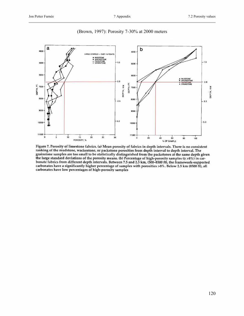
Jon Petter Furnée 7 Appendix 7.2 Porosity values
120
(Brown, 1997): Porosity 7-30% at 2000 meters

Jon Petter Furnée 7 Appendix 7.2 Porosity values
121
(Brown, 1997): Porosity 5% at 2000 meters

Jon Petter Furnée 7 Appendix 7.2 Porosity values
122
(Brown, 1997): Porosity 5-20% at 2000 meters

Jon Petter Furnée 7 Appendix 7.3 Example of .data-file in Eclipse
123
7.3 Example of .data-file in Eclipse NOECHO
-- ==================================================================================================
--
-- Lowcase_cave_rc10
--
-- Exported by user jonfor from RMS2013 at 2015-03-17 11:33:41
--
-- ==================================================================================================
-- ==================================================================================================
RUNSPEC
-- ==================================================================================================
TITLE
Lowcase_cave_rc10
-- --------------------------------------------------------------------------------------------------
-- Grid dimensions
-- --------------------------------------------------------------------------------------------------
DIMENS
-- NX NY NZ
261 279 35 /
-- --------------------------------------------------------------------------------------------------
-- Simulation start date
-- --------------------------------------------------------------------------------------------------
START
1 'JAN' 2014 /
-- --------------------------------------------------------------------------------------------------
-- Unit system
-- --------------------------------------------------------------------------------------------------
METRIC
-- --------------------------------------------------------------------------------------------------
-- Phases and components
-- --------------------------------------------------------------------------------------------------
OIL
WATER

Jon Petter Furnée 7 Appendix 7.3 Example of .data-file in Eclipse
124
-- --------------------------------------------------------------------------------------------------
-- Program dimensions
-- --------------------------------------------------------------------------------------------------
-- Equilibration dimensions
EQLDIMS
-- NTEQUL NDPRVD NDRXVD
1 100 20 /
-- Linear solver stack size. NSTACK is set equal to LITMAX if enough memory on computer. See keyword under “tuning parameters” below.
NSTACK
100 /
-- Number of iterations to update well targets (got a warning that said that I had too increase the value from 3)
NUPCOL
10 /
-- Table dimensions
TABDIMS
-- NTSFUN NTPVT NSSFUN NPPVT NTFIP NRPVT
1 1 40 30 30 30 /
-- Well dimensions
WELLDIMS
-- NWMAXZ NCWMAX NGMAXZ NWGMAX
5 20 5 5 /
-- Fault dimensions
FAULTDIM
-- MFSEGS
0 /
-- --------------------------------------------------------------------------------------------------
-- Path names
-- --------------------------------------------------------------------------------------------------
PATHS
'MAIN' 'C:\Users\jonfor\Dropbox\UIB\Master\Setergrotta_E\Lowcase_cave_rc10' /
/

Jon Petter Furnée 7 Appendix 7.3 Example of .data-file in Eclipse
125
-- --------------------------------------------------------------------------------------------------
-- Options
-- --------------------------------------------------------------------------------------------------
-- Data checking only
--NOSIM
-- Input/output options
-- UNIFIN -- Unified input files
UNIFOUT -- Unified output files
-- Grid options
GRIDOPTS
YES /
-- ==================================================================================================
GRID
-- ==================================================================================================
-- --------------------------------------------------------------------------------------------------
-- Output control
-- --------------------------------------------------------------------------------------------------
-- Grid file export
GRIDFILE
-- GRID EGRID
0 1 /
-- Init file export
INIT
RPTGRID
-- ALLNNC
-- DEPTH
-- DX
-- DY
-- DZ
-- FAULTS
-- PORO
-- PORV
-- NTG
-- PERMX
-- PERMY

Jon Petter Furnée 7 Appendix 7.3 Example of .data-file in Eclipse
126
-- PERMZ
-- TRANX
-- TRANY
-- TRANZ
/
-- --------------------------------------------------------------------------------------------------
-- Grid definition
-- --------------------------------------------------------------------------------------------------
MAPAXES
269.549 69.087
269.549 719.138
682.200 719.138
/
MAPUNITS
METRES /
GRIDUNIT
METRES /
GDORIENT
INC INC INC DOWN LEFT /
INCLUDE
'$MAIN\Lowcase_cave_rc10.coord.inc'
/
INCLUDE
'$MAIN\Lowcase_cave_rc10.zcorn.inc'
/
INCLUDE
'$MAIN\Lowcase_cave_rc10.actnum.inc'
/

Jon Petter Furnée 7 Appendix 7.3 Example of .data-file in Eclipse
127
-- --------------------------------------------------------------------------------------------------
-- Petrophysical properties
-- --------------------------------------------------------------------------------------------------
-- Porosity
INCLUDE
'$MAIN\Lowcase_cave_rc10.poro.inc'
/
-- Net-to-gross
INCLUDE
'$MAIN\Lowcase_cave_rc10.ntg.inc'
/
-- X Permeability
INCLUDE
'$MAIN\Lowcase_cave_rc10.permx.inc'
/
-- Y Permeability
INCLUDE
'$MAIN\Lowcase_cave_rc10.permy.inc'
/
-- Z Permeability
INCLUDE
'$MAIN\Lowcase_cave_rc10.permz.inc'
/

Jon Petter Furnée 7 Appendix 7.3 Example of .data-file in Eclipse
128
-- ==================================================================================================
PROPS
-- ==================================================================================================
-- --------------------------------------------------------------------------------------------------
-- Output control
-- --------------------------------------------------------------------------------------------------
RPTPROPS
-- PVTO
-- PVDG or PVTG
-- PVTW
-- SGFN
-- SOFN
-- SWFN
-- SGL
-- SGU
-- SGCR
-- SOGCR
-- SOWCR
-- SWL
-- SWU
-- SWCR
-- PCG
-- PCW
-- ROCK
/

Jon Petter Furnée 7 Appendix 7.3 Example of .data-file in Eclipse
129
-- --------------------------------------------------------------------------------------------------
-- Fluid data
-- --------------------------------------------------------------------------------------------------
-- Two-phase (water-oil) relative permeability curves.
-- Relativ permeability for water and oil, and capillary pressure as a function of water saturation.
-- Sw – Water saturation, Krw – Relative permeability for water, Kro – Relative permeability for oil, Pcow – Capillary pressure
SWOF
-- Sw Krw Kro Pcow
0.200 0.000 0.850 0
0.250 0.006 0.727 0
0.300 0.013 0.613 0
0.350 0.022 0.509 0
0.400 0.032 0.414 0
0.450 0.043 0.330 0
0.500 0.057 0.255 0
0.550 0.071 0.189 0
0.600 0.087 0.133 0
0.650 0.105 0.087 0
0.700 0.124 0.051 0
0.750 0.144 0.024 0
0.800 0.167 0.007 0
0.850 0.190 0.000 0
0.900 0.300 0.000 0
1.000 1.000 0.000 0 /
-- PVT-data for water
-- Pref – Reference pressure for rest of data, Bw – Volume formation factor for water, Cw – Water compressibility, ViscW – Water viscosity,
-- Cv – Viscobility
PVTW
-- Pref Bw Cw ViscW Cv
308.2 1.024 0.0000464 0.42 1* /

Jon Petter Furnée 7 Appendix 7.3 Example of .data-file in Eclipse
130
-- PVT-data for dead oil (black oil)
-- P(bar) – Pressure in Bar, Bo – Volume formation factor for oil, ViscO – Oil viscosity
PVDO
-- P(bar) Bo ViscO
227.00 1.2600 1.042
253.40 1.2555 1.072
281.60 1.2507 1.096
311.10 1.2463 1.118
343.80 1.2417 1.151
373.50 1.2377 1.174
395.50 1.2356 1.200 /
-- Rock compressibility (linear)
-- Pref – Reference pressure for rest of data, Cr – Rock compressibility
ROCK
-- Pref Cr
1 5.60E-05 /
-- Surface densities [kg/Sm3]
DENSITY
-- oil Water Gas
833 1038 0.66 /
-- Oil is always above bubble-point-pressure, i.e. dead oil, no free gas => Rs is constant
-- Rs – Dissolved gas concentration
RSCONST
-- Rs Bubble-point-pressure
100 180 /

Jon Petter Furnée 7 Appendix 7.3 Example of .data-file in Eclipse
131
-- ==================================================================================================
REGIONS
-- ==================================================================================================
-- --------------------------------------------------------------------------------------------------
-- Output control
-- --------------------------------------------------------------------------------------------------
RPTREGS
-- PVTNUM
-- SATNUM
-- EQLNUM
-- FIPNUM
/
-- --------------------------------------------------------------------------------------------------
-- Region grid arrays
-- --------------------------------------------------------------------------------------------------
-- Fluid data regions
INCLUDE
'$MAIN\Lowcase_cave_rc10.pvtnum.inc'
/
-- Saturation data regions
INCLUDE
'$MAIN\Lowcase_cave_rc10.satnum.inc'
/
-- Equilibrium data regions
INCLUDE
'$MAIN\Lowcase_cave_rc10.eqlnum.inc'
/
-- Fluid-in-place data regions
INCLUDE
'$MAIN\Lowcase_cave_rc10.fipnum.inc'
/

Jon Petter Furnée 7 Appendix 7.3 Example of .data-file in Eclipse
132
-- ==================================================================================================
SOLUTION
-- ==================================================================================================
-- --------------------------------------------------------------------------------------------------
-- Output control
-- --------------------------------------------------------------------------------------------------
RPTSOL
'RESTART = 2' -- Initial restart kept
'FIP=1' -- Fluid in place for whole field
-- DENG
-- DENO
-- DENS
-- DENW
-- EQUIL
-- FIPRESV
-- FLOGAS
-- FLOOIL
-- FLOWAT
-- KRG
-- KRO
-- KRW
-- PVDPH
-- RPORV
/
-- --------------------------------------------------------------------------------------------------
-- Equilibration data
-- --------------------------------------------------------------------------------------------------
-- Equilibration data
-- Datum – Datum depth, Pdatum – Pressure at the datum depth, OWC – Oil water contact (defined below the reservoir to get it completely
-- oil-filled, with no mobile water present in the reservoir), PCOWC – Capillary pressure at the contact, GOC – Gas oil contact (defined above
-- the reservoir to avoid including gas in model), PCGOC – Gas-oil capillary pressure at the gas-oil contact (default 0), TRSVD – Integer
-- selecting the type of initialization for live black oil (default 0), TRVVD – Integer selecting the type of initialization for black oil runs with wet
-- gas (default 0)
EQUIL
-- Datum Pdatum OWC PCOWC GOC PCGOC TRSVD TRVVD /
1859.02 300 2096.89 0 1859.02 0 0 0 /

Jon Petter Furnée 7 Appendix 7.3 Example of .data-file in Eclipse
133
-- ==================================================================================================
SUMMARY
-- ==================================================================================================
ALL
-- View in Excel
EXCEL
-- Field Pressure Rate
FPR
-- Field Oil Production Rate
FOPR
-- Field Water Production Rate
FWPR
-- Field Gas Production Rate
FGPR
-- Field Oil Production Total
FOPT
-- Field Water Production Total
FWPT
-- Field Gas Production Total
FGPT
-- Field Oil Efficiency
FOE
-- To compare run times
-- Time step length
TIMESTEP
-- Number of Newton iterations for each time step
NEWTON
-- Current CPU usage in seconds
TCPU
-- CPU time per time step in seconds
TCPUTS
-- CPU time per day
TCPUDAY
-- Average number of linear iterations per Newton iteration, for each time step
NLINEARS

Jon Petter Furnée 7 Appendix 7.3 Example of .data-file in Eclipse
134
-- ==================================================================================================
SCHEDULE
-- ==================================================================================================
-- Define frequency for writing of restart files (every 1 month)
RPTRST
BASIC=5 NORST=1 FREQ=1 /
-- Well specifications
WELSPECS
-- Wname Gname Iwh Jwh Z(bhp) PrefPhase 2* ShutIn XFlowFlag
-- 1* DensCalc FIPnr /
WP1 G 117 142 1* OIL /
WI1 G 233 22 1* WAT /
WI2 G 27 261 1* WAT /
/
-- Completion data
COMPDAT
-- Wnm* Ic Jc K_top K_btm Open/Shut SatTblNbr tfac Rh(diam) Kh
-- Skin dfac penDir r0 /
WP1 117 142 16 29 O 1* 1* 0.35 1*
0 1* Z 1* /
WI1 233 22 15 25 O 1* 1* 0.35 1*
0 1* Z 1* /
WI2 27 261 14 24 O 1* 1* 0.35 1*
0 1* Z 1* /
/
-- Production specification. Specify a rate that ideally would drain the whole reservoir in 10 years.
-- 373582 Sm3 oil in place / 10 years / 365 days = 100 Sm3/day
WCONPROD
-- Wnm* Open/ShutFlag Ctrlmode Orat Wrat Grat Lrat Resv) BHPmin THPmin VFP-data
WP1 OPEN ORAT 100 1* 1* 300 1* 180 1* 1* /
/

Jon Petter Furnée 7 Appendix 7.3 Example of .data-file in Eclipse
135
-- Injection data
WCONINJE
-- Wnm* InjFluid Open/Shut CtrlMode Rate Resv BHP THP 1* /
WI1 WATER OPEN RATE 50 1* 500 1* 1* /
WI2 WATER OPEN RATE 50 1* 500 1* 1* /
/
GCONINJE
-- Group Phase CtrlMode RateTrg RvolTrg ReinjTrg VoidReplFrac /
FIELD WATER VREP 1* 1* 1* 0.9999 /
/
-- --------------------------------------------------------------------------------------------------
-- Output control
-- --------------------------------------------------------------------------------------------------
RPTSCHED
-- 'RESTART=2' -- All restarts kept
-- 'FIP=1' -- Fluid in place for whole field
-- PRES
-- SOIL
-- SWAT
-- RS
-- RV
-- WELLS
-- SUMMARY
-- CPU
-- NEWTON
/
-- --------------------------------------------------------------------------------------------------
-- Tuning parameters
-- --------------------------------------------------------------------------------------------------
-- LITMAX specifies the maximum number of linear iterations in a Newton iteration. To avoid the calculations to run circles, a high enough
-- NSTACK has to be set. Usual these two are set equal.
TUNING
-- TSINIT TSMAXZ TSMINZ TSMCHP TSFMAX TSFMIN TSFCNV TFDIFF /
0.1 5 0.1 1* 1* 1* 1* 1* /
-- TRGTTE TRGCNV TRGMBE TRGLCV XXXTTE XXXMBE XXXLCV XXXWFL /
1* 1* 1* 1* 1* 1* 1* 1* /
-- NEWTMX NEWTMN LITMAX LITMIN MXWSIT MXWPIT DDPLIM DDSLIM /
40 1 100 1 1* 1* 1* 1* /

Jon Petter Furnée 7 Appendix 7.3 Example of .data-file in Eclipse
136
-- --------------------------------------------------------------------------------------------------
-- Time control
-- --------------------------------------------------------------------------------------------------
-- List of report dates (15 years from production start 1. Jan 2014).
DATES
1 FEB 2014 / -- 1. YEAR
1 MAR 2014 / -- 1. YEAR
1 APR 2014 / -- 1. YEAR
1 MAY 2014 / -- 1. YEAR
1 JUN 2014 / -- 1. YEAR
1 JUL 2014 / -- 1. YEAR
1 AUG 2014 / -- 1. YEAR
1 SEP 2014 / -- 1. YEAR
1 OCT 2014 / -- 1. YEAR
1 NOV 2014 / -- 1. YEAR
1 DEC 2014 / -- 1. YEAR
1 JAN 2015 / -- 2. YEAR
1 FEB 2015 / -- 2. YEAR
1 MAR 2015 / -- 2. YEAR
1 APR 2015 / -- 2. YEAR
1 MAY 2015 / -- 2. YEAR
1 JUN 2015 / -- 2. YEAR
1 JUL 2015 / -- 2. YEAR
1 AUG 2015 / -- 2. YEAR
1 SEP 2015 / -- 2. YEAR
1 OCT 2015 / -- 2. YEAR
1 NOV 2015 / -- 2. YEAR
1 DEC 2015 / -- 2. YEAR
1 JAN 2016 / -- 3. YEAR
1 FEB 2016 / -- 3. YEAR
1 MAR 2016 / -- 3. YEAR
1 APR 2016 / -- 3. YEAR
1 MAY 2016 / -- 3. YEAR
1 JUN 2016 / -- 3. YEAR
1 JUL 2016 / -- 3. YEAR
1 AUG 2016 / -- 3. YEAR
1 SEP 2016 / -- 3. YEAR
1 OCT 2016 / -- 3. YEAR

Jon Petter Furnée 7 Appendix 7.3 Example of .data-file in Eclipse
137
1 NOV 2016 / -- 3. YEAR
1 DEC 2016 / -- 3. YEAR
1 JAN 2017 / -- 4. YEAR
1 FEB 2017 / -- 4. YEAR
1 MAR 2017 / -- 4. YEAR
1 APR 2017 / -- 4. YEAR
1 MAY 2017 / -- 4. YEAR
1 JUN 2017 / -- 4. YEAR
1 JUL 2017 / -- 4. YEAR
1 AUG 2017 / -- 4. YEAR
1 SEP 2017 / -- 4. YEAR
1 OCT 2017 / -- 4. YEAR
1 NOV 2017 / -- 4. YEAR
1 DEC 2017 / -- 4. YEAR
1 JAN 2018 / -- 5. YEAR
1 FEB 2018 / -- 5. YEAR
1 MAR 2018 / -- 5. YEAR
1 APR 2018 / -- 5. YEAR
1 MAY 2018 / -- 5. YEAR
1 JUN 2018 / -- 5. YEAR
1 JUL 2018 / -- 5. YEAR
1 AUG 2018 / -- 5. YEAR
1 SEP 2018 / -- 5. YEAR
1 OCT 2018 / -- 5. YEAR
1 NOV 2018 / -- 5. YEAR
1 DEC 2018 / -- 5. YEAR
1 JAN 2019 / -- 6. YEAR
1 FEB 2019 / -- 6. YEAR
1 MAR 2019 / -- 6. YEAR
1 APR 2019 / -- 6. YEAR
1 MAY 2019 / -- 6. YEAR
1 JUN 2019 / -- 6. YEAR
1 JUL 2019 / -- 6. YEAR
1 AUG 2019 / -- 6. YEAR
1 SEP 2019 / -- 6. YEAR
1 OCT 2019 / -- 6. YEAR
1 NOV 2019 / -- 6. YEAR
1 DEC 2019 / -- 6. YEAR

Jon Petter Furnée 7 Appendix 7.3 Example of .data-file in Eclipse
138
1 JAN 2020 / -- 7. YEAR
1 FEB 2020 / -- 7. YEAR
1 MAR 2020 / -- 7. YEAR
1 APR 2020 / -- 7. YEAR
1 MAY 2020 / -- 7. YEAR
1 JUN 2020 / -- 7. YEAR
1 JUL 2020 / -- 7. YEAR
1 AUG 2020 / -- 7. YEAR
1 SEP 2020 / -- 7. YEAR
1 OCT 2020 / -- 7. YEAR
1 NOV 2020 / -- 7. YEAR
1 DEC 2020 / -- 7. YEAR
1 JAN 2021 / -- 8. YEAR
1 FEB 2021 / -- 8. YEAR
1 MAR 2021 / -- 8. YEAR
1 APR 2021 / -- 8. YEAR
1 MAY 2021 / -- 8. YEAR
1 JUN 2021 / -- 8. YEAR
1 JUL 2021 / -- 8. YEAR
1 AUG 2021 / -- 8. YEAR
1 SEP 2021 / -- 8. YEAR
1 OCT 2021 / -- 8. YEAR
1 NOV 2021 / -- 8. YEAR
1 DEC 2021 / -- 8. YEAR
1 JAN 2022 / -- 9. YEAR
1 FEB 2022 / -- 9. YEAR
1 MAR 2022 / -- 9. YEAR
1 APR 2022 / -- 9. YEAR
1 MAY 2022 / -- 9. YEAR
1 JUN 2022 / -- 9. YEAR
1 JUL 2022 / -- 9. YEAR
1 AUG 2022 / -- 9. YEAR
1 SEP 2022 / -- 9. YEAR
1 OCT 2022 / -- 9. YEAR
1 NOV 2022 / -- 9. YEAR
1 DEC 2022 / -- 9. YEAR
1 JAN 2023 / -- 10. YEAR
1 FEB 2023 / -- 10. YEAR

Jon Petter Furnée 7 Appendix 7.3 Example of .data-file in Eclipse
139
1 MAR 2023 / -- 10. YEAR
1 APR 2023 / -- 10. YEAR
1 MAY 2023 / -- 10. YEAR
1 JUN 2023 / -- 10. YEAR
1 JUL 2023 / -- 10. YEAR
1 AUG 2023 / -- 10. YEAR
1 SEP 2023 / -- 10. YEAR
1 OCT 2023 / -- 10. YEAR
1 NOV 2023 / -- 10. YEAR
1 DEC 2023 / -- 10. YEAR
1 JAN 2024 / -- 11. YEAR
1 FEB 2024 / -- 11. YEAR
1 MAR 2024 / -- 11. YEAR
1 APR 2024 / -- 11. YEAR
1 MAY 2024 / -- 11. YEAR
1 JUN 2024 / -- 11. YEAR
1 JUL 2024 / -- 11. YEAR
1 AUG 2024 / -- 11. YEAR
1 SEP 2024 / -- 11. YEAR
1 OCT 2024 / -- 11. YEAR
1 NOV 2024 / -- 11. YEAR
1 DEC 2024 / -- 11. YEAR
1 JAN 2025 / -- 12. YEAR
1 FEB 2025 / -- 12. YEAR
1 MAR 2025 / -- 12. YEAR
1 APR 2025 / -- 12. YEAR
1 MAY 2025 / -- 12. YEAR
1 JUN 2025 / -- 12. YEAR
1 JUL 2025 / -- 12. YEAR
1 AUG 2025 / -- 12. YEAR
1 SEP 2025 / -- 12. YEAR
1 OCT 2025 / -- 12. YEAR
1 NOV 2025 / -- 12. YEAR
1 DEC 2025 / -- 12. YEAR
1 JAN 2026 / -- 13. YEAR
1 FEB 2026 / -- 13. YEAR
1 MAR 2026 / -- 13. YEAR
1 APR 2026 / -- 13. YEAR

Jon Petter Furnée 7 Appendix 7.3 Example of .data-file in Eclipse
140
1 MAY 2026 / -- 13. YEAR
1 JUN 2026 / -- 13. YEAR
1 JUL 2026 / -- 13. YEAR
1 AUG 2026 / -- 13. YEAR
1 SEP 2026 / -- 13. YEAR
1 OCT 2026 / -- 13. YEAR
1 NOV 2026 / -- 13. YEAR
1 DEC 2026 / -- 13. YEAR
1 JAN 2027 / -- 14. YEAR
1 FEB 2027 / -- 14. YEAR
1 MAR 2027 / -- 14. YEAR
1 APR 2027 / -- 14. YEAR
1 MAY 2027 / -- 14. YEAR
1 JUN 2027 / -- 14. YEAR
1 JUL 2027 / -- 14. YEAR
1 AUG 2027 / -- 14. YEAR
1 SEP 2027 / -- 14. YEAR
1 OCT 2027 / -- 14. YEAR
1 NOV 2027 / -- 14. YEAR
1 DEC 2027 / -- 14. YEAR
1 JAN 2028 / -- 15. YEAR
1 FEB 2028 / -- 15. YEAR
1 MAR 2028 / -- 15. YEAR
1 APR 2028 / -- 15. YEAR
1 MAY 2028 / -- 15. YEAR
1 JUN 2028 / -- 15. YEAR
1 JUL 2028 / -- 15. YEAR
1 AUG 2028 / -- 15. YEAR
1 SEP 2028 / -- 15. YEAR
1 OCT 2028 / -- 15. YEAR
1 NOV 2028 / -- 15. YEAR
1 DEC 2028 / -- 15. YEAR
1 JAN 2029 / -- END
/
END

Jon Petter Furnée 7 Appendix

Jon Petter Furnée 7 Appendix
CD contains:
PDF version of the Master Thesis
RMS model
One Eclipse simulation model (Lowcase_cave_rc10)