fluid dynamics and heat transfer in a hartmann flow
TRANSCRIPT

i
Fluid Dynamics and Heat Transfer in a Hartmann Flow
by
Timothy Richard DePuy
An Engineering Project Submitted to the Graduate
Faculty of Rensselaer Polytechnic Institute
in Partial Fulfillment of the
Requirements for the degree of
MASTER OF ENGINEERING IN MECHANICAL ENGINEERING
Approved:
_________________________________________
Ernesto Gutierrez, Project Adviser
Rensselaer Polytechnic Institute
Hartford, Connecticut
December, 2010

ii
CONTENTS
LIST OF SYMBOLS ........................................................................................................ iii
LIST OF TABLES ............................................................................................................ iv
LIST OF FIGURES ........................................................................................................... v
ABSTRACT ..................................................................................................................... vi
1. Introduction .................................................................................................................. 1
2. Methodology ................................................................................................................ 2
2.1 Governing Equations .......................................................................................... 2
2.2 Solution Method ................................................................................................. 5
2.2.1 Lorentz Force Solution ........................................................................... 5
2.2.2 Hydrodynamic Flow Solution ................................................................ 7
2.2.3 Heat Transfer Solution ........................................................................... 9
2.3 Expected Results .............................................................................................. 10
3. Results and Discussion .............................................................................................. 12
3.1 Lorentz Force Solution ..................................................................................... 12
3.2 Fluid Flow Solution ......................................................................................... 14
3.3 Heat Transfer Solution ..................................................................................... 15
4. Conclusions................................................................................................................ 19
4.1 Applicability of COMSOL to MHD Flows ..................................................... 19
4.2 Heat Transfer in Hartmann Flows .................................................................... 20
5. References .................................................................................................................. 21
6. Appendix A: Additional Graphs of Solutions ........................................................... 22

iii
LIST OF SYMBOLS
D, Electric Displacement Field (C/m2)
e , Free Charge Density (C/m)
P, Pressure (Pa)
f, , Viscosity (Pa*s)
H, Magnetizing Field (A/m)
J, zx JJ , , Current Density (A/m2)
0 , Magnetic Permeability (N/A2)
M, Hartmann Number
V,u,v,w, Velocity (m/s)
B, zx BBB ,,0 , Magnetic Fields (T)
E, zx EE , , Electric Field (N/C)
, Electrical Conductivity of the Fluid (S/m)
bF , Body Force (N)
Dh, Hydraulic Diameter (m)
Re, Reynolds Number
Pr, Prandtl Number
q , Heat Flux (W/m2)
T, Temperature (K)
, Density (kg/m3)
pc , Heat Capacity (J/(kg*K))
k, Thermal Conductivity (W/(m*K))
h, Convective Heat Transfer Coefficient (W/(m2*K))
i , Static Enthalpy (J)
j , Mass Diffusion Coefficient
jm , Mass Concentration
Q , Heat Source (J)

iv
LIST OF TABLES
Table 1. Applicable Fluid Properties of Mercury at 523K ................................................ 5
Table 2. Conditions Used to Evaluate the Lorentz Force Contribution ............................ 6
Table 3. Conditions Used to Evaluate the Fluid Velocities ............................................... 8
Table 4. Conditions Used to Evaluate the Magnetic and Hydrodynamic Models ........... 12
Table 5. Post-processed Heat Transfer Results ............................................................... 18
Table 6. Nusselt Numbers for Parallel Plate Flow Versus Entry Length ........................ 18

v
LIST OF FIGURES
Figure 1. Electric and Magnetic Fields Applied to a Pressure Driven Parallel Plate Flow 2
Figure 2. Meshed Domain ................................................................................................. 5
Figure 3. Applied Magnetostatics Boundary Conditions .................................................. 6
Figure 4. Iterative Solution Method ................................................................................... 7
Figure 5. Applied Fluid Dynamics Boundary Conditions ................................................. 7
Figure 6. Transition to Turbulence in Hartmann Flows [9]............................................... 9
Figure 7. Applied Boundary Conditions for the Heat Transfer Analysis .......................... 9
Figure 8. Calculated and Exact Lorentz Force Solutions ................................................ 13
Figure 9. Analytical and Computed Velocity Profiles for Various Hartmann Numbers . 14
Figure 10. Normalized Computed Velocity Profiles for Various Hartmann Numbers ... 15
Figure 11. Surface Temperature over the Analyzed Fluid Domain for M=0 .................. 16
Figure 12. Calculated Heat Flux for Various Hartmann Numbers .................................. 16
Figure 13. Heat Flux Normalized to Case 0 .................................................................... 17
Figure 14. Pressure over the Analyzed Fluid Domain ..................................................... 19

vi
ABSTRACT
Steady state channel flow of an electrically conductive liquid exposed to transverse
magnetic and electric fields was analyzed using a finite element model in COMSOL
Multiphysics software to determine the flow velocities and heat transfer characteristics
of the flow. The Lorentz force, velocity profile, and Nusselt number results were
compared to the available exact solutions for this Hartmann flow problem. A range of
dimensionless Hartmann numbers in the laminar region was analyzed numerically as
well as analytically, and the solutions were compared.
1
1. Introduction
Magnetohydrodynamics (MHD) is a field that has many applications in metallurgy,
microfluidic pumping, power generation in fusion and fission reactors, and cosmic
studies. The ability to control the flow of liquid metal and plasmas at high temperatures
through magnetic fields without mechanical influence has novel applications. Liquid
metal flows can be manipulated with the magnetic field producing effects such as
electromagnetic braking that is widely used in the continuous casting of steel, [1].
Additionally, MHD has proven to be an efficient pumping method in microfluidic
devices whose scale would typically require significant pressure gradients to achieve
adequate flow rates, [2]. A specific type of MHD flow that has been studied extensively
is flow in a channel between two parallel plates, known as Hartmann flow. Analytical
solutions have been obtained for the flow profile and heat transfer characteristics.
Numerical solutions can be obtained through finite element analysis of the magnetic
field and flow.
For this project, the flow of a steady state incompressible liquid metal between parallel
plates in a transverse magnetic field was analyzed. The plates were assumed to be
electrically insulated so as to not influence the magnetic field. A pressure was applied to
the inlet of the channel, and a Lorentz body force due to the magnetic field was
calculated. The Lorentz force altered the flow profile and consequently the heat transfer
characteristics of the flow. The change in heat transfer rate with respect to the change in
flow profile due to the Lorentz force was analyzed.

2
2. Methodology
2.1 Governing Equations
The Maxwell and Navier-Stokes equations can be solved using the COMSOL
Multiphysics analysis software and compared to theoretical solutions found in references
[3], [4], and [5]. The problem that was analyzed is shown in Figure 1. The parallel
plates were separated by a distance of 2y0. A magnetic field was applied in the upward
y-direction. A differential pressure between the inlet and outlet of the plates was applied
so that a flow profile that varies in the y-direction develops. The pressure gradient in the
z-direction was chosen as zero so that flow only occurred in the x-direction. The
magnetic field created an electromotive force on the fluid as it moved between the
plates.
Figure 1. Electric and Magnetic Fields Applied to a Pressure Driven Parallel Plate Flow
The governing equations for this problem are derived from the Maxwell equations,
Ohm’s law, and the Navier-Stokes equations. The electromotive force needs to be
applied as a body force in the Navier-Stokes equations so that the effect of the magnetic
field on the fluid is included in the fluid flow solution.
The Maxwell Equations were taken from [5]:
e D
0 B
t
BE
t
DJH
This was combined with Ohm’s Law:
))(( BVEJ
B
E
x
y
2y
00
0
u(y) Po Pi

3
In order to derive an analytical solution from the above equations, certain assumptions
must be made. The constitutive equation, HB 0 , is assumed accurate for liquid
metals and gases in most MHD problems, although it is not true in general for all types
of flows. This, along with the assumption that induced magnetic fields are much smaller
than the externally applied magnetic field and that t /D is negligible are the three
major assumptions used to reduce the Maxwell equations to an MHD approximation
form. These assumptions are generally valid for most ordinary conductors at relative
low velocities (V << speed of sound). As shown in detail in Chapter 6 of [5], Maxwell’s
equations can be reduced using these assumptions to:
t
BE
JH
0 J
0 B
))(( BVEJ
These equations are coupled with the incompressible Navier-Stokes equations (Chapter
4 of [5]) through the J and B fields which appear as a body force:
bpt
FVVVV
2
Where BJF b
For the parallel plate problem, the left side of the equation equals zero because velocities
in the y and z directions are zero, the velocities are time invariant, and the velocity
profile does not change with x. Likewise many terms on the right hand side are zero,
and the equations simplify to:
xf
zxxz
zf
JBy
w
z
p
BJBJy
p
JBy
u
x
p
02
2
02
2
0
0
0
Using Ohm’s Law:

4
)(
)(
0
0
uBEJ
wBEJ
zz
xx
Since we have chosen the flow (and pressure gradient) to be in the x-direction, the w,
xJ , xE , and zp / are zero and the above equations are reduced to the one equation
shown below:
)(0 002
2
uBEBy
u
x
pzf
This is a representation of a simple one dimensional parallel plate flow with an applied
body force dependent upon the applied electrical and magnetic fields. This equation can
be used to solve for the velocity profile between the plates by applying appropriate
boundary conditions which are discussed in a later section.
The general energy equation from [6] is solved in order to calculate the temperature
distribution and heat flux in the fluid and through the boundaries:
SDt
DPmiTk
Dt
Di
j
jjj
where j
i
ij
l
l
i
j
j
i
x
u
x
u
x
u
x
u
3
2
These equations are rearranged in COMSOL assuming time invariance and no
dissipation so that Conduction = Source – Convection:
TcQTk p V
After COMSOL solved the above equation, the results were post-processed to solve for
the convective heat transfer coefficient.
bs TT
qh
where
0
0
0
0
y
y
y
y
b
dyu
dyTu
T
The convective heat transfer coefficient was used to determine the Nusselt Number.

5
2.2 Solution Method
2.2.1 Lorentz Force Solution
COMSOL Multiphysics was used to create a magnetostatics model of a channel with
conductive fluid flow exposed to magnetic and electric fields. The obtained solutions
are compared to the analytical solutions for the Lorentz force and fluid velocity shown in
the following section. Mercury was selected as the conductive fluid due to its
applicability to MHD (a conductive metal that is often used and studied because it is
liquid at room temperatures). Fluid properties at 523.15K from [7] were used because
the heat transfer was analyzed at temperatures close to this temperature. These
properties are presented in Table 1.
Electrical
Conductivity
Dynamic
Viscosity Density
Thermal
Conductivity Heat capacity
1 x 10⁶ S/m 0.001 Pa*s 13026 kg/m
3 13.07 W/(m*K) 136 J/(kg*K)
Table 1. Applicable Fluid Properties of Mercury at 523K
The flat plates were separated by a distance of 10 centimeters. The length of the
modeled plates was 6 meters, which is a sufficient condition to match the assumption
used in the analytical solution, that the length is much greater than the distance between
the plates. The model was meshed using the built in COMSOL meshing functions. A
fine mesh of 23552 triangular elements was used:
Figure 2. Meshed Domain
An electrical insulation boundary condition was applied to the border of the domain as
this was assumed in the analytical solution. The boundary conditions are shown in
Figure 3.
6
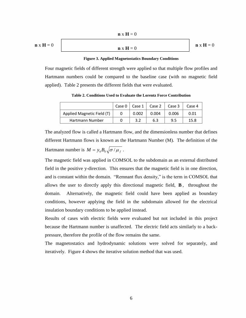
Figure 3. Applied Magnetostatics Boundary Conditions
Four magnetic fields of different strength were applied so that multiple flow profiles and
Hartmann numbers could be compared to the baseline case (with no magnetic field
applied). Table 2 presents the different fields that were evaluated.
Table 2. Conditions Used to Evaluate the Lorentz Force Contribution
Case 0 Case 1 Case 2 Case 3 Case 4
Applied Magnetic Field (T) 0 0.002 0.004 0.006 0.01
Hartmann Number 0 3.2 6.3 9.5 15.8
The analyzed flow is called a Hartmann flow, and the dimensionless number that defines
different Hartmann flows is known as the Hartmann Number (M). The definition of the
Hartmann number is fByM /00 .
The magnetic field was applied in COMSOL to the subdomain as an external distributed
field in the positive y-direction. This ensures that the magnetic field is in one direction,
and is constant within the domain. “Remnant flux density,” is the term in COMSOL that
allows the user to directly apply this directional magnetic field, B , throughout the
domain. Alternatively, the magnetic field could have been applied as boundary
conditions, however applying the field in the subdomain allowed for the electrical
insulation boundary conditions to be applied instead.
Results of cases with electric fields were evaluated but not included in this project
because the Hartmann number is unaffected. The electric field acts similarly to a back-
pressure, therefore the profile of the flow remains the same.
The magnetostatics and hydrodynamic solutions were solved for separately, and
iteratively. Figure 4 shows the iterative solution method that was used.
n x H = 0 n x H = 0
n x H = 0
n x H = 0
7
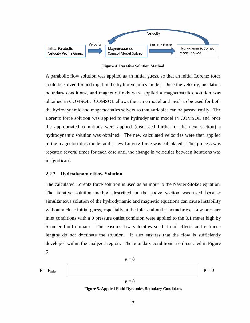
Figure 4. Iterative Solution Method
A parabolic flow solution was applied as an initial guess, so that an initial Lorentz force
could be solved for and input in the hydrodynamics model. Once the velocity, insulation
boundary conditions, and magnetic fields were applied a magnetostatics solution was
obtained in COMSOL. COMSOL allows the same model and mesh to be used for both
the hydrodynamic and magnetostatics solvers so that variables can be passed easily. The
Lorentz force solution was applied to the hydrodynamic model in COMSOL and once
the appropriated conditions were applied (discussed further in the next section) a
hydrodynamic solution was obtained. The new calculated velocities were then applied
to the magnetostatics model and a new Lorentz force was calculated. This process was
repeated several times for each case until the change in velocities between iterations was
insignificant.
2.2.2 Hydrodynamic Flow Solution
The calculated Lorentz force solution is used as an input to the Navier-Stokes equation.
The iterative solution method described in the above section was used because
simultaneous solution of the hydrodynamic and magnetic equations can cause instability
without a close initial guess, especially at the inlet and outlet boundaries. Low pressure
inlet conditions with a 0 pressure outlet condition were applied to the 0.1 meter high by
6 meter fluid domain. This ensures low velocities so that end effects and entrance
lengths do not dominate the solution. It also ensures that the flow is sufficiently
developed within the analyzed region. The boundary conditions are illustrated in Figure
5.
Figure 5. Applied Fluid Dynamics Boundary Conditions
P = Pinlet P = 0
v = 0
v = 0

8
No slip wall conditions were applied to the upper and lower plates. The calculated
Lorentz force from the magnetostatics solution was applied as a body force to the fluid
domain. Different pressures were applied to each case so that the volumetric flow rate
between the plates differed by less than 1% between cases. Increased pressures were
applied at higher Hartmann numbers to achieve the same flow rate because the Lorentz
force acts against the flow. The entrance region affects the linearity of the pressure
drop; therefore trial and error was used to get the desired pressure drop per meter in the
fully developed region. At higher Hartmann numbers the entrance length is reduced,
therefore the analytical equations were used to estimate the required inlet pressure for
cases 3 and 4. The following inlet pressures were used:
Table 3. Conditions Used to Evaluate the Fluid Velocities
Case 0 Case 1 Case 2 Case 3 Case 4
Applied Inlet Pressure (Pa) 0.006 0.023 0.071 0.149 0.395
Hartmann Number 0 3.2 6.3 9.5 15.8
The velocities that result from these pressures ensured that the flow is laminar. Figure 6,
taken from [8], shows that as the Hartmann number increases, the flow becomes more
stable and requires a much higher Reynolds number to transition to turbulent flow. For
pressure driven parallel plate flow, transition to turbulent flow is expected to occur at a
Reynolds number of 2000, [9]. The Reynolds number for Case 0 is 600 and less for the
other cases, therefore laminar flow was present in all cases.

9
Figure 6. Transition to Turbulence in Hartmann Flows [9]
Once the boundary conditions and Lorentz forces were applied to the model, the
hydrodynamic problem was solved. As described above, the magnetostatics and
hydrodynamic solution were solved iteratively until new solutions stopped changing
significantly.
2.2.3 Heat Transfer Solution
The forced convection heat transfer solution was obtained by applying the boundary
conditions specified in Figure 7 to the geometries in COMSOL.
Figure 7. Applied Boundary Conditions for the Heat Transfer Analysis
The fully developed analytical fluid flow solutions were used in the heat transfer
analysis so that flow entrance effects would not affect the solution. A shorter geometry,
0.1 meter high by 2 meter long fluid domain, was used for the heat transfer solution
because the domain quickly reached the wall temperature. The walls were held at a
Constant Ts < Ti
Constant Ts < Ti
Flow Solution
Convective
Heat Flux Ti = 573K
10
constant temperature (323.15 K) and the fluid entered at a constant inlet temperature
(573.15 K). A convective heat flux boundary condition was applied to the outlet. An
additional domain was used for the region from 0 meters to 0.2 meters so that the
temperature profile can be integrated in COMSOL at 0.2 meters and a bulk temperature
could be determined.
The solutions for each case were compared to determine how the flow profile affects the
heat transfer between parallel plates. The Nusselt number was used to determine how
the Hartmann number affected the heat transfer rate.
The heating that occurs when the magnetic field is applied to the flow was not included
in this analysis because the effect of flow profile on the heat transfer was desired.
Reference [3] describes a steady state solution where this heating is set equal to the heat
lost through the walls.
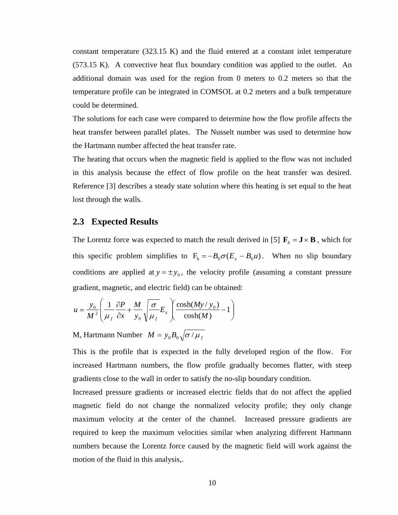
2.3 Expected Results
The Lorentz force was expected to match the result derived in [5] BJF b , which for
this specific problem simplifies to )(F 00b uBEB z . When no slip boundary
conditions are applied at 0yy , the velocity profile (assuming a constant pressure
gradient, magnetic, and electric field) can be obtained:
1
)cosh(
)/cosh(1 0
0
2
0
M
yMyE
y
M
x
P
M
yu z
ff
M, Hartmann Number fByM /00
This is the profile that is expected in the fully developed region of the flow. For
increased Hartmann numbers, the flow profile gradually becomes flatter, with steep
gradients close to the wall in order to satisfy the no-slip boundary condition.
Increased pressure gradients or increased electric fields that do not affect the applied
magnetic field do not change the normalized velocity profile; they only change
maximum velocity at the center of the channel. Increased pressure gradients are
required to keep the maximum velocities similar when analyzing different Hartmann
numbers because the Lorentz force caused by the magnetic field will work against the
motion of the fluid in this analysis,.
11
It can be expected that the heat transfer for the higher Hartmann number flows of the
same volumetric flow rate will be increased due to the increase flow near the wall
boundary. Increased convection would be expected because the increase in velocity is
near the boundary. The point of greatest heat flux at the inlet is at the walls (since the
wall temperature is held constant.) The dimensionless Nusselt number is a common
parameter used to characterize the convective heat transfer for a specific type of flow.
As described in [10], for the baseline condition with no magnetic field (Case 0) the
expected Nusselt number is 7.54. Laminar fully developed flow in a rectangular cross
section pipe of infinite width is assumed for this theoretical result. Case 0 is used to
confirm accuracy of solution and conformance to theory. The other cases were
compared to this result to examine the change in heat transfer rate. Nusselt numbers will
be calculated for each case.

12
3. Results and Discussion
3.1 Lorentz Force Solution
The magnetostatics finite element modeling module of COMSOL Multiphysics was used
to determine the Lorentz force for a Hartmann flow described by the boundary
conditions shown in Figure 3. A 2-dimensional 0.1 meter high, 6 meter long domain was
analyzed with the applied magnetic fields and hydrodynamic solutions described in
section 2.2 and repeated in the Table 4.
Table 4. Conditions Used to Evaluate the Magnetic and Hydrodynamic Models
Case 0 Case 1 Case 2 Case 3 Case 4
Applied Inlet Pressure (Pa) 0.006 0.023 0.071 0.149 0.395
Applied Magnetic Field (T) 0 0.002 0.004 0.006 0.01
Hartmann Number 0 3.2 6.3 9.5 15.8
The hydrodynamic and magnetic solutions were solved iteratively since the velocity
affects the magnetic solution, and the Lorentz force affects the velocities. As shown in
Figure 8, with an increasing Hartmann number, the Lorentz force increases and matches
the expected results. The lines represent the exact solution described in section 2.3. The
dots are the results of the COMSOL model.

13
Figure 8. Calculated and Exact Lorentz Force Solutions
The body force is divided by the length of the channel to determine the equivalent back
pressure that is being applied to the fluid. Toward the middle of the channel, the force
almost negates the applied pressure force, which results in very low velocities in the
channel when compared to a solution with no applied magnetic field. Figure 8 confirms
that the analytical Lorentz body force )( 00 uBEB z matches the calculated results.
Therefore this term can be directly used in the fluid flow solution so that the magnetic
solution does not need to be recalculated or solved iteratively. However, for more
complicated flows with non-uniform fields such a simple term may not be readily
available or determined, therefore the iterative method used in this project is a more
powerful solution method for more general, realistic flows.

14
3.2 Fluid Flow Solution
The calculated velocity profiles for a pressure driven flow for the cases described in
Table 4 are shown in Figure 9. These profiles have approximately the same volumetric
flow rate (within 1%).
Figure 9. Analytical and Computed Velocity Profiles for Various Hartmann Numbers
As the magnetic field was increased, the Lorentz force also increased, which reduces the
velocity throughout the channel. The Lorentz force is a function of velocity, therefore
the normally parabolic flow receives a greater counter-flow force at the highest velocity
points (center of the channel). As the magnitude of the magnetic field increases, the
force in the center increases until the flow becomes almost constant through the channel
(except very close to the walls so the solution satisfies the no slip boundary condition).
Contour plots of the pressure field combined with an arrow plot of the velocity field for
each of the analyzed cases are shown in Appendix A. The velocities normalized to the
maximum velocity are shown in Figure 10.
15
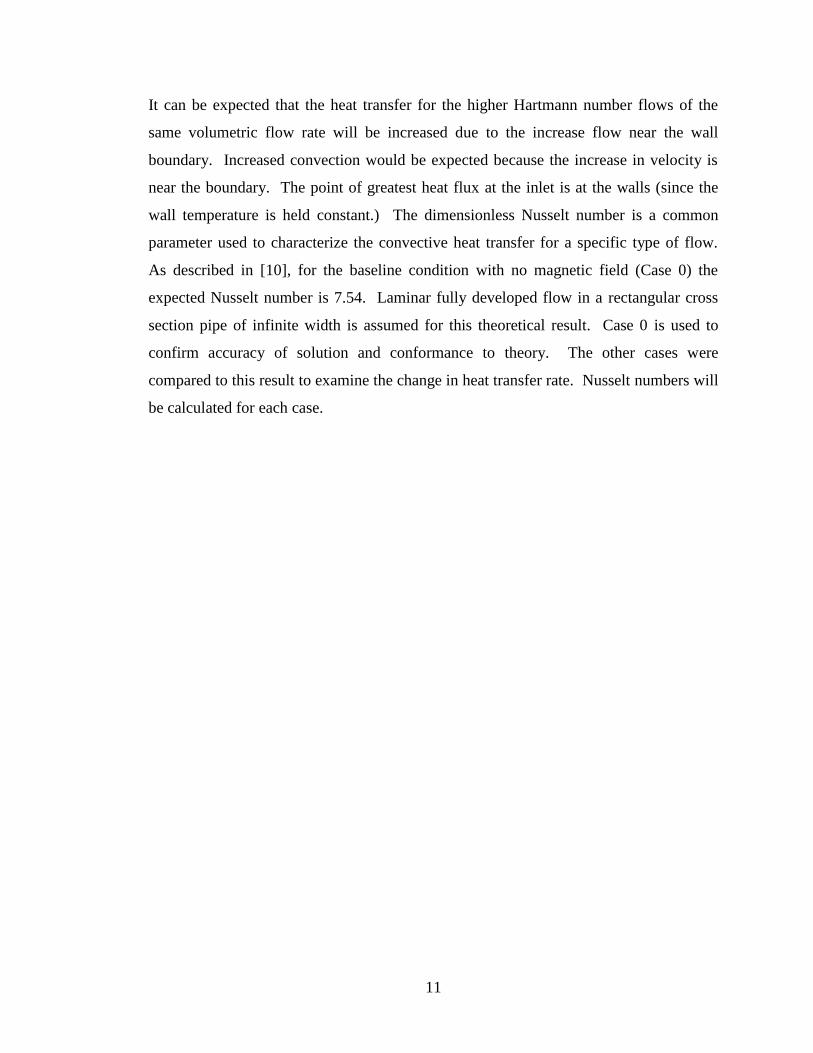
Figure 10. Normalized Computed Velocity Profiles for Various Hartmann Numbers
As shown in Figure 10, the effects of the magnetic field become more pronounced as the
field increases. Even at the moderate Hartmann numbers used in this project, the
velocity profile is nearly flat. Hartmann numbers for many industrial and laboratory
applications can be large (M = 10 – 10000), [11]. For these flows the velocity profile is
practically constant between the plates.
3.3 Heat Transfer Solution
The heat transfer analysis described in Section 2.2.3 was performed. As expected, the
heat transfer was enhanced at higher Hartmann numbers with volumetric flow rate held
constant. A contour plot of the fluid temperatures for the baseline Case 0 with no
applied magnetic field is shown in Figure 11.

16
Figure 11. Surface Temperature over the Analyzed Fluid Domain for M=0
The temperature contour plots for cases 1-4 were similar to the baseline case. The heat
fluxes through the wall for each case are plotted together in Figure 12.
Figure 12. Calculated Heat Flux for Various Hartmann Numbers

17
As shown in the Figure, the heat flux is slightly enhanced with increasing Hartmann
Number. Since the heat transfer is enhanced, the temperatures in the fluid domain more
quickly reach the wall temperature. A crossover point at approximately 0.08 meters is
due to the lower difference in bulk temperature and wall temperature. This is shown
more clearly in a normalized plot, Figure 13.
Figure 13. Heat Flux Normalized to Case 0
Figure 13 shows the heat fluxes normalized to the baseline Case 0. Ignoring the end
effect, the heat flux amplification is a maximum at the beginning of the domain, where
temperatures between cases are almost identical due to the inlet temperature boundary
condition. Due to the larger heat flux, Cases 1-4 cool faster than Case 0. At ≈ 0.08
meters the Hartmann flow cases have cooled to a point where the decreased temperature
difference has counteracted the increased heat transfer coefficient, and the overall heat
flux is equivalent to the baseline case. The overall heat transfer throughout the domain,
however, has been greater.
The heat flux and temperatures were exported from the COMSOL program and post-
processed in Microsoft Excel to determine the heat transfer coefficient and Nusselt
number. Applicable heat transfer parameters for the solution at x = 0.2 meters (which is

18
at the edge of the thermal entry length region) are shown in Table 5. This short distance
was chosen because the fluid domain quickly reaches the wall temperature due to the
relatively high heat transfer coefficient.
Table 5. Post-processed Heat Transfer Results
Case 0 Case 1 Case 2 Case 3 Case 4
Surface Temperature Tinf (K) 373.15 373.15 373.15 373.15 373.15
Heat Flux q'' (W/m2) 17415 16526 15444 14787 14117
Bulk Temperature Tbulk (K) 408.31 404.99 401.47 399.60 397.89
Heat Transfer Coefficient h (W/m2*K) 495.3 519.0 545.3 559.1 570.6
Nusselt Number Nu 7.579 7.941 8.344 8.555 8.731
The Nusselt number exact solution for a parabolic pressure driven channel flow with a
constant wall temperature is Nu = 7.54, [10]. Table 8-9 from [6] shows that a slightly
increased Nusselt number is expected in this region of flow. The dimensionless entry
length (x+) is 0.033 for Case 0. As shown in Table 6, the calculated Nusselt number is
reasonable for the baseline case.
Table 6. Nusselt Numbers for Parallel Plate Flow Versus Entry Length
X+ = 2*(x/Dh)/RePr Nu
0.01 8.52
0.02 7.75
0.05 7.55
0.1 7.55
0.2 7.55
The computed Nusselt number for Case 0 is very close to the exact Nusselt number
which gives confidence that the model is accurately predicting the temperature
distribution and heat flux in the fluid.

19
4. Conclusions
4.1 Applicability of COMSOL to MHD Flows
The results obtained using COMSOL to model a pressure driven parallel plate flow
exposed to an external magnetic field were compared to theory and analytical solutions.
Convergence issues were encountered when trying to solve both the magnetic and
hydrodynamic solutions simultaneously, however when solved iteratively the solutions
converged easily. It was discovered that, entrance and end effects can have large
influences on both the convergence and the accuracy of the solution. A graph of the
pressure on the centerline of the channel for the baseline case with no magnetic field
shows that the pressure loss in the entrance region is not linear.
Figure 14. Pressure over the Analyzed Fluid Domain
The purpose of this project was to analyze fully developed flow; therefore the inlet
pressure was adjusted until the desired pressure drop in the fully developed region was
Entrance region

20
achieved. According to [6], the entrance length for parallel plate flow is calculated to be
0.05*Re*D, which for the baseline flow, Case 0, would be approximately 3 meters. The
measured pressure gradient in the 4 to 6 meter region was therefore used in the exact
solutions. The velocities and resulting Reynolds number in this analysis were chosen to
be small so that the entrance length of the flow could be kept small. This resulted in
some of the analyzed region being fully developed. In the fully developed region, the
COMSOL results matched the analytical solutions for the Lorentz force and velocity
profile. Given the accuracy of the results obtained from this analysis, it is expected that
other Hartmann flows modeled in COMSOL for different conductive fluids would yield
accurate results given an appropriate domain size and mesh resolution. Also, it is
expected that more complicated MHD flows could be analyzed in COMSOL by using
the iterative method that was used to evaluate the flows in this report.
4.2 Heat Transfer in Hartmann Flows
As expected, slightly enhanced heat transfer was obtained at higher Hartmann numbers.
This enhancement may be beneficial in flows where magnetic fields are used for braking
because Joule heating can cause the temperature of the fluid to rise rapidly. Typically
the conductive heat transfer coefficient for liquid metal flows is large, therefore the
slight enhancement in heat transfer may be insignificant for practical applications.
However for temperature critical applications, the change in Nusselt number for
different Hartmann numbers needs to be taken into consideration.
21
5. References
[1] Egbert Zienicke, Thomas Boeck, and Dmitry Krasnov, Transition to Turbulence in
Magnetohydrodynamic Channel Flow of Liquid Metals, NIC Series, Vol. 32 (2006),
p. 341-348.
[2] Asuncion V. Lemoff and Abraham P. Lee, An AC Magnetohydrodynamic
Micropump, Sensors and Actuators B: Chemical Vol. 63, Issue 3 (2000), p. 178-
185.
[3] Elmārs Blūms, Yu. A. Mikhailov and R. Ozols, Heat and Mass Transfer in MHD
Flows, World Scientific Publishing, 1987.
[4] R. A. Alpher, Heat Transfer in Magnetohydrodynamic Flow Between Parallel
Plates, International Journal of Heat and Mass Transfer Vol. 3 Issue 2 (1961), p.
108-112.
[5] W. F. Hughes and F. J. Young, The Electromagnetodynamics of Fluids, John Wiley
& Sons, New York:1966.
[6] William Kays et. all, Convective Heat and Mass Transfer Fourth Edition, McGraw-
Hill, Boston: 2005.
[7] Mercury- Properties, The Engineering ToolBox,
http://www.engineeringtoolbox.com/mercury-d_1002.html
[8] S. Smolentsev and R. Moreau, Modeling quasi-two-dimensional turbulence in MHD
duct flows, Center for Turbulence Research Proceedings of the Summer Program
2006 p. 419-430.
[9] Frank M. White, Viscous Fluid Flow Third Edition, MaGraw-Hill, New York: 2006.
[10] Frank P. Incropera et. all, Fundamentals of Heat and Mass Transfer 6th
Edition, John
Wiley & Sons, 2007.
[11] J. C. R. Hunt and R. Moreau, Liquid-metal magnetohydrodynamics with strong
magnetic fields: a report on Euromech 70, Journal of Fluid Mechanics, Vol. 78
(1976), p. 261-288.

22
6. Appendix A: Additional Graphs of Solutions

23
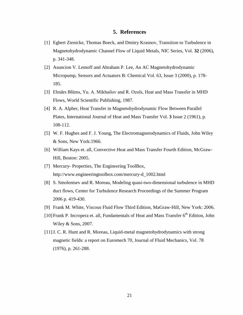
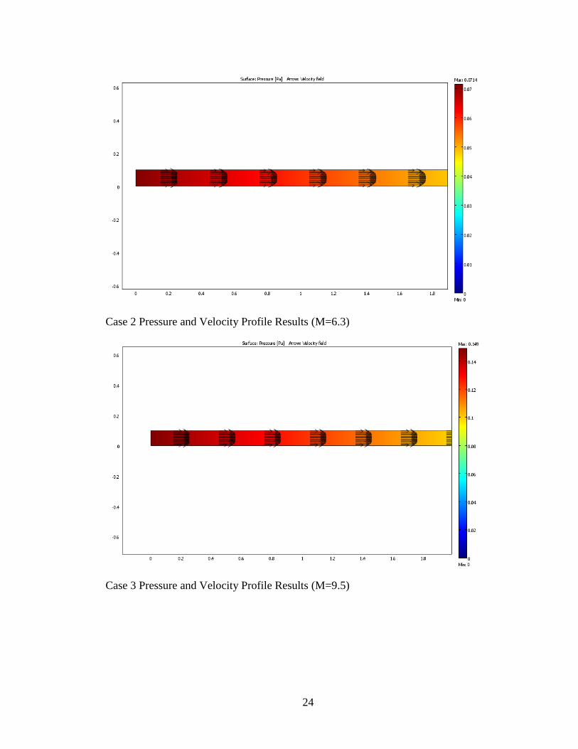
Contour plots showing the pressure and arrow plots showing the velocity profile for
cases 0-4 are shown below. The change in velocity to a flatter profile can be seen.
Additionally, the entry length as the Hartmann number increases gets shorter.
Case 0 Pressure and Velocity Profile Results (M=0)
Case 1 Pressure and Velocity Profile Results (M=3.2)
24
Case 2 Pressure and Velocity Profile Results (M=6.3)
Case 3 Pressure and Velocity Profile Results (M=9.5)

25
Case 4 Pressure and Velocity Profile Results (M=15.8)