2

“COMPUTATIONAL FLUID DYNAMICS USING ANSYS

FLUENT”

A SEMINAR REPORT

Submitted by

Aditya Karan

Roll No. 301003 Exam No. T8230002

Of

Third Year Civil Engineering

Guided by

Asst. Prof. G.A.Hinge

SINHGAD COLLEGE OF ENGINEERING,

VADGAON Bk., PUNE-41

2

CERTIFICATE

This i s to cer t i fy that the Seminar work “ COMPUTATIONAL

FLUID DYNAMICS USING ANSYS FLUENT” i s a seminar done by

Adi tya Karan under my guidance in par t ia l fu l f i l lment o f the

requirements for the Bachelors in Engineer ing (Civi l )

SIGNATURE SIGNATURE

Dr. Mrs. K .C. Khare Asst. Prof. G.A.Hinge

HEAD OF THE DEPARTMENT SEMINAR GUIDE

Department of Civil Engineering Department of Civil Engineering

Sinhagad College Of Engineering; Sinhagad College Of Engineering;

Vadgaon, Pune-41. Vadgaon, Pune-41.

2

ACKNOWLEDGEMENTS

I take immense pleasure in thanking Dr. Mrs. K.C. Khare , our Head of the department, for

having permitted me to carry out this seminar work.

I wish to express my deep sense of gratitude to my Guide, Asst. Prof. Mr.G.A.Hinge,

Sinhagad College Of Engineering Vadgaon Bk. , Pune-41

for his able guidance and useful suggestions, which helped me in completing the seminar

work, in time.

Finally, yet importantly, I would like to express my heartfelt thanks to my beloved parents

for their blessings, my friends/classmates for their help and wishes for the successful

completion of this project.

Aditya Karan

2

TABLE OF CONTENTS

CHAPTER NO. TITLE PAGE NO.

ABSTRACT i

1. BACKGROUND-FLUIDS 6

2. INTRODUCTION TO COMPUTATIONAL 10

FLUID DYNAMICS

2.1 METHODOLOGY 10

2.2 DISCRETION METHODS 11

2.2.1 FINITE VOLUME METHOD

2.2.2 FINITE ELEMENT METHOD

2.2.3 REYNOLDS-AVERAGED NAVIER STOKES

2.2.4 LARGE EDDY SIMULATION

2.2.5 DIRECT NUMERICAL SIMULATION

2.3 EXAMPLES 12

3 INTRODUCTION TO SOFTWARE. 13

3.1 INTRODUTION TO GAMBIT 14

3.2 INTRODUCTION TO FLUENT 15

3.3 GENERATING A SIMPLE 2-D MODEL 16

3.4 MODELLING OF 3-D OPEN CHANNEL MODEL 24.

3.5 MODELLING OF 2-D CAVITIES. 29

3.6

4.0 CASE STUDY 30

4.1 CONCLUSION OF SURGE ANALYSIS. 33

5.0 CONCLUSION OF THE SEMINAR 34

REFERENCES. 35

2

ABSTRACT:

The study of fluids is vital for our understanding of the world. Traditionally this was done through studying

fluid flow on models in something like a wind tunnel, but in the last century the field of computational fluid

dynamics has come into being. One program that is capable of modeling fluid flow is Fluent. The aim of

this project was to model a few scenarios using Fluent. The purpose of doing so was to see how accurate the

program was at modeling fluid flow in order to see if computational fluid dynamics has advanced enough to

do away with the traditional methods. A tutorial for Gambit and Fluent is included as an introduction which

illustrates the basic features of these tools will able to create their own case studies in CFD.

Computational fluid dynamics is a term used to describe a way of modeling fluids using algorithms and

numerical methods. Currently they are solved utilizing computers but early methods were completed

manually without the aid of a computer. Computational fluid dynamics are a powerful tool to model fluids,

but even with the most state of the art supercomputers and technological advances they are only an

approximation of what would occur in reality. A number of different problems in CFD are examined in

more detail.

2

1.0 Background - Fluids

In this section, I sketch an algebraic approach to fluids and indicate its connections to the fuller differential

approach. The intent is to introduce the fundamental equations which are solved in numerical simulations

alongside with a means of understanding the important features of these equations at the pre-calculus high

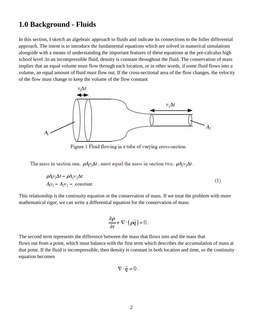
school level .In an incompressible fluid, density is constant throughout the fluid. The conservation of mass

implies that an equal volume must flow through each location, or in other words, if some fluid flows into a

volume, an equal amount of fluid must flow out. If the cross-sectional area of the flow changes, the velocity

of the flow must change to keep the volume of the flow constant

This relationship is the continuity equation or the conservation of mass. If we treat the problem with more

mathematical rigor, we can write a differential equation for the conservation of mass:

The second term represents the difference between the mass that flows into and the mass that

flows out from a point, which must balance with the first term which describes the accumulation of mass at

that point. If the fluid is incompressible, then density is constant in both location and time, so the continuity

equation becomes

2

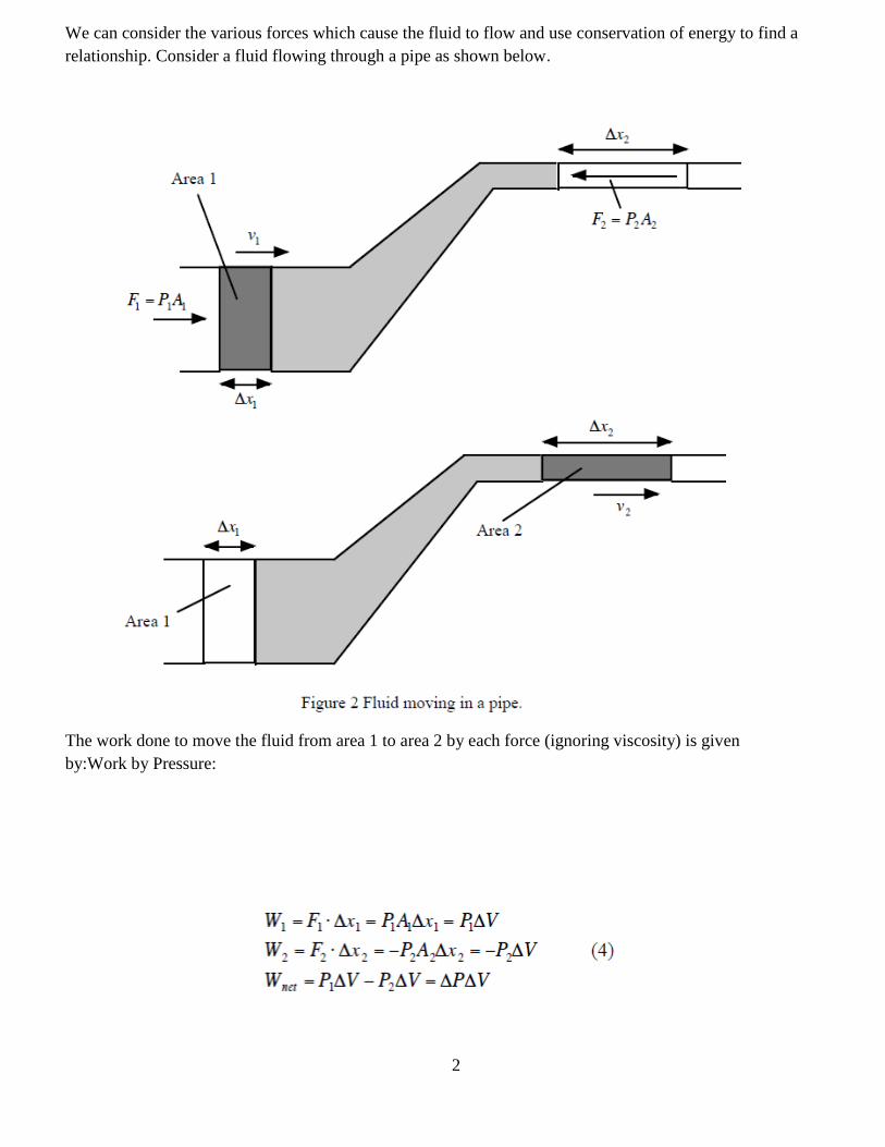
We can consider the various forces which cause the fluid to flow and use conservation of energy to find a

relationship. Consider a fluid flowing through a pipe as shown below.

The work done to move the fluid from area 1 to area 2 by each force (ignoring viscosity) is given

by:Work by Pressure:

2

A key feature to note from the pressure equation (4) is that flow is driven by a difference in

pressure between the points, with the fluid moving from areas of higher pressure to areas of

lower pressure (“favorable pressure difference”).

Work by Gravity:

The mass in each section is given by

So the net work to raise the fluid from area 1 to area 2 is

Conservation of energy implies that the change in the kinetic energy of the fluid is equal to the work done

on the fluid,

Simplifying and rearranging the terms, we have the Bernoulli Equation (for a nonviscous fluid):

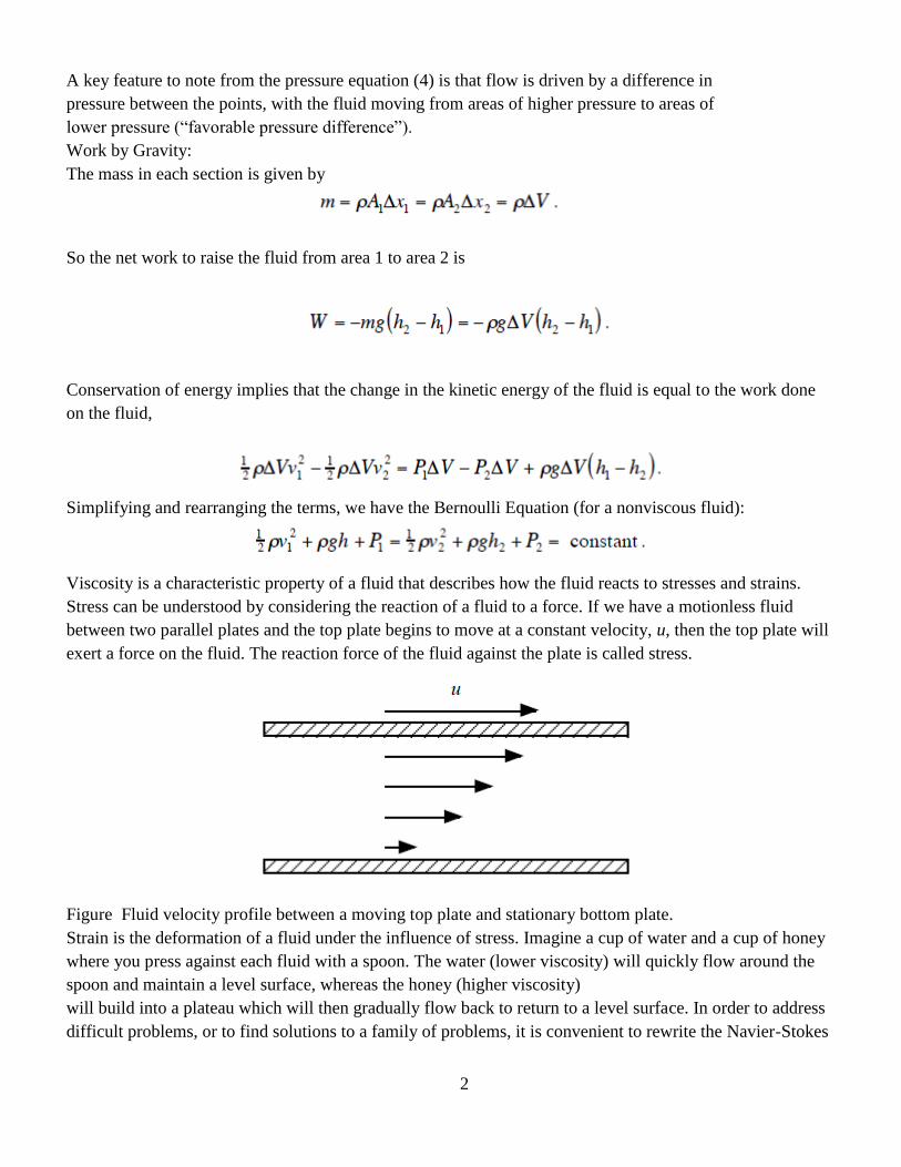
Viscosity is a characteristic property of a fluid that describes how the fluid reacts to stresses and strains.

Stress can be understood by considering the reaction of a fluid to a force. If we have a motionless fluid

between two parallel plates and the top plate begins to move at a constant velocity, u, then the top plate will

exert a force on the fluid. The reaction force of the fluid against the plate is called stress.

Figure Fluid velocity profile between a moving top plate and stationary bottom plate.

Strain is the deformation of a fluid under the influence of stress. Imagine a cup of water and a cup of honey

where you press against each fluid with a spoon. The water (lower viscosity) will quickly flow around the

spoon and maintain a level surface, whereas the honey (higher viscosity)

will build into a plateau which will then gradually flow back to return to a level surface. In order to address

difficult problems, or to find solutions to a family of problems, it is convenient to rewrite the Navier-Stokes

2

equations in dimensionless form. In doing so, it is necessary introduce a number of “characteristic”

quantities, such as

ρ density

u characteristic velocity (such as inflow)

L characteristic length (such as the length of an object in your flow)

Viscosity

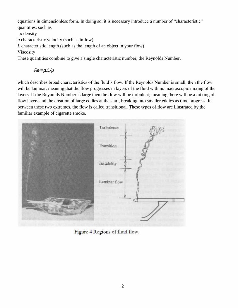
These quantities combine to give a single characteristic number, the Reynolds Number,

Re =ρuL/μ

which describes broad characteristics of the fluid’s flow. If the Reynolds Number is small, then the flow

will be laminar, meaning that the flow progresses in layers of the fluid with no macroscopic mixing of the

layers. If the Reynolds Number is large then the flow will be turbulent, meaning there will be a mixing of

flow layers and the creation of large eddies at the start, breaking into smaller eddies as time progress. In

between these two extremes, the flow is called transitional. These types of flow are illustrated by the

familiar example of cigarette smoke.

2

2.0 Introduction to Computational Fluid Dynamics

The equations for fluids are quite complex and can be difficult to solve, especially if the geometry of a

problem is intricate. The equations are nonlinear in the acceleration term (convection term),have

singularities for high Reynolds Numbers (which appears in the N-S equations in the form of 1\Re), and the

pressure difference terms are difficult to solve in combination with the fluid’s motion. By making use of

computers as a computational tool, we can “solve” these equations of motion in nearly any arbitrary

situation. In this particular work, Gambit is used to create the geometries and the computational grid for the

problem. This allows us to move from working with the fluid as a continuous medium to a discrete

approach. Fluent ,a finite volume solver, is used to solve the discrete Navier-Stokes equations. Some of the

results of interesting cases are given below. The computational method allows us to get results quickly (a

matter of minutes to hours depending on the complexity) and visually close to reality. These results can be

used to guide experiments and even as a substitute for preliminary testing in situations where building

prototypes might be prohibitively expensive.

Computational fluid dynamics, usually abbreviated as CFD, is a branch of fluid mechanics

that uses numerical methods and algorithms to solve and analyze problems that involve fluid flows.

Computers are used to perform the calculations required to simulate the interaction of liquids and gases with

surfaces defined by boundary conditions. With high-speed supercomputers, better solutions can be achieved.

Ongoing research yields software that improves the accuracy and speed of complex simulation scenarios

such as transonic or turbulent flows. Initial validation of such software is performed using a wind tunnel

with the final validation coming in full-scale testing.

2.1Methodology

In all of these approaches the same basic procedure is followed.

During preprocessing

o The geometry (physical bounds) of the problem is defined.

o The volume occupied by the fluid is divided into discrete cells (the mesh). The mesh may be

uniform or non uniform.

o The physical modeling is defined – for example, the equations of motions + enthalpy +

radiation + species conservation Boundary conditions are defined. This involves specifying

o the fluid behaviour and properties at the boundaries of the problem. For transient problems,

the initial conditions are also defined.

The simulation is started and the equations are solved iteratively as a steady-state or transient.

Finally a postprocessor is used for the analysis and visualization of the resulting solution.

2.2 Discretization methods

The stability of the chosen discretization is generally established numerically rather than analytically as with

simple linear problems. Special care must also be taken to ensure that the discretization handles

2

discontinuous solutions gracefully. The Euler equations and Navier–Stokes equations both admit shocks,

and contact surfaces.

Some of the discretization methods being used are:

2.2.1Finite volume method

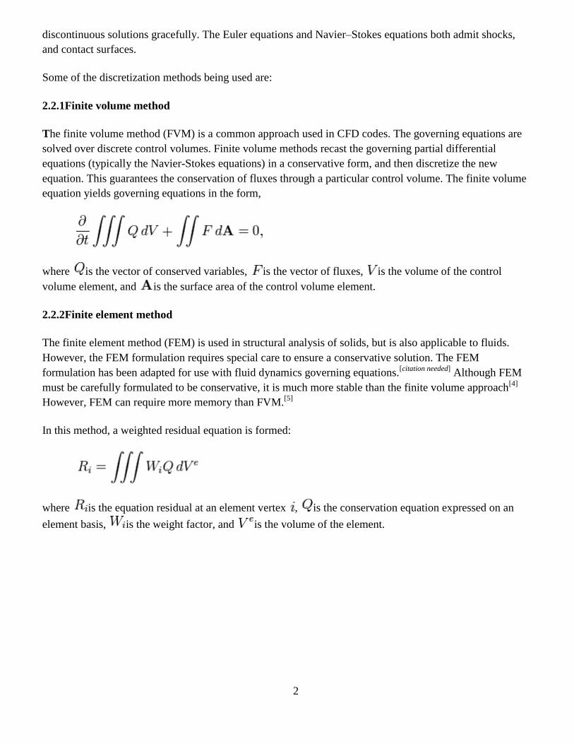
The finite volume method (FVM) is a common approach used in CFD codes. The governing equations are

solved over discrete control volumes. Finite volume methods recast the governing partial differential

equations (typically the Navier-Stokes equations) in a conservative form, and then discretize the new

equation. This guarantees the conservation of fluxes through a particular control volume. The finite volume

equation yields governing equations in the form,

where is the vector of conserved variables, is the vector of fluxes, is the volume of the control

volume element, and is the surface area of the control volume element.

2.2.2Finite element method

The finite element method (FEM) is used in structural analysis of solids, but is also applicable to fluids.

However, the FEM formulation requires special care to ensure a conservative solution. The FEM

formulation has been adapted for use with fluid dynamics governing equations.[citation needed]

Although FEM

must be carefully formulated to be conservative, it is much more stable than the finite volume approach[4]

However, FEM can require more memory than FVM.[5]

In this method, a weighted residual equation is formed:

where is the equation residual at an element vertex , is the conservation equation expressed on an

element basis, is the weight factor, and is the volume of the element.

2

2.2.3 Reynolds-averaged Navier–Stokes

Reynolds-averaged Navier-Stokes (RANS) equations are the oldest approach to turbulence modeling. An

ensemble version of the governing equations is solved, which introduces new apparent stresses known as

Reynolds stresses. This adds a second order tensor of unknowns for which various models can provide

different levels of closure. It is a common misconception that the RANS equations do not apply to flows

with a time-varying mean flow because these equations are 'time-averaged'. In fact, statistically unsteady (or

non-stationary) flows can equally be treated. This is sometimes referred to as URANS. There is nothing

inherent in Reynolds averaging to preclude this, but the turbulence models used to close the equations are

valid only as long as the time over which these changes in the mean occur is large compared to the time

scales of the turbulent motion containing most of the energy.

RANS models can be divided into two broad approaches:

Boussinesq hypothesis

This method involves using an algebraic equation for the Reynolds stresses which include

determining the turbulent viscosity, and depending on the level of sophistication of the model, solving

transport equations for determining the turbulent kinetic energy and dissipation. Models include k-ε

(Launder and Spalding), Mixing Length Model (Prandtl), and Zero Equation Model (Cebeci and Smith) The

models available in this approach are often referred to by the number of transport equations associated with

the method. For example, the Mixing Length model is a "Zero Equation" model because no transport

equations are solved; the is a "Two Equation" model because two transport equations (one for and

one for ) are solved.

Reynolds stress model (RSM)

This approach attempts to actually solve transport equations for the Reynolds stresses. This means

introduction of several transport equations for all the Reynolds stresses and hence this approach is much

more costly in CPU effort.

2.2.4 Large eddy simulation

Large eddy simulation (LES) is a technique in which the smallest scales of the flow are removed through a

filtering operation, and their effect modeled using subgrid scale models. This allows the largest and most

important scales of the turbulence to be resolved, while greatly reducing the computational cost incurred by

the smallest scales. This method requires greater computational resources than RANS methods, but is far

cheaper than DNS.

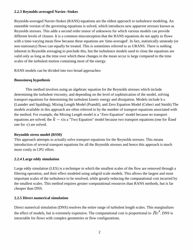
2.2.5 Direct numerical simulation

Direct numerical simulation (DNS) resolves the entire range of turbulent length scales. This marginalizes

the effect of models, but is extremely expensive. The computational cost is proportional to . DNS is

intractable for flows with complex geometries or flow configurations.

2

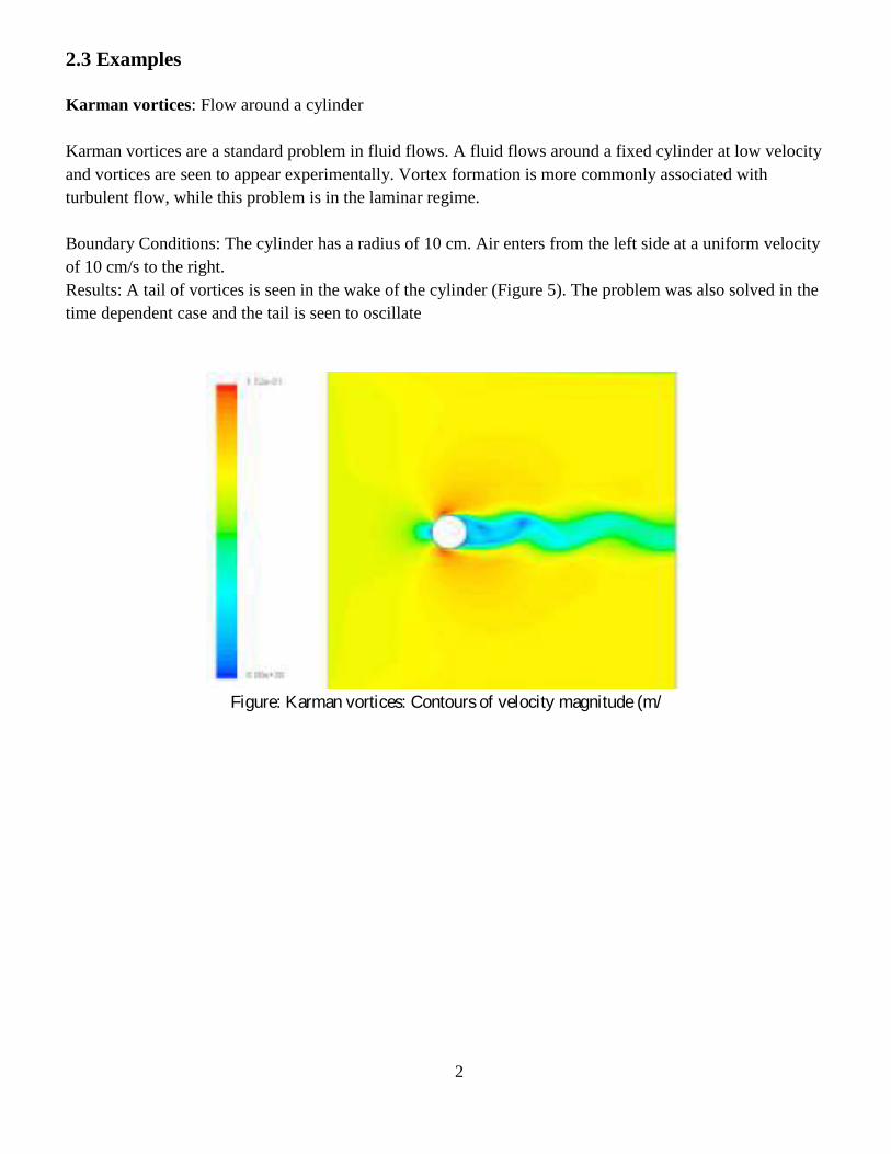
2.3 Examples

Karman vortices: Flow around a cylinder

Karman vortices are a standard problem in fluid flows. A fluid flows around a fixed cylinder at low velocity

and vortices are seen to appear experimentally. Vortex formation is more commonly associated with

turbulent flow, while this problem is in the laminar regime.

Boundary Conditions: The cylinder has a radius of 10 cm. Air enters from the left side at a uniform velocity

of 10 cm/s to the right.

Results: A tail of vortices is seen in the wake of the cylinder (Figure 5). The problem was also solved in the

time dependent case and the tail is seen to oscillate

Figure: Karman vortices: Contours of velocity magnitude (m/

2

3.0 INTRODUTION TO THE SOFTWARE :

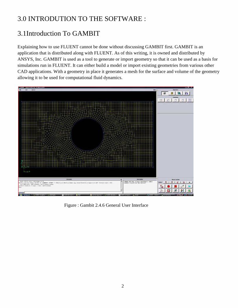
3.1Introduction To GAMBIT

Explaining how to use FLUENT cannot be done without discussing GAMBIT first. GAMBIT is an

application that is distributed along with FLUENT. As of this writing, it is owned and distributed by

ANSYS, Inc. GAMBIT is used as a tool to generate or import geometry so that it can be used as a basis for

simulations run in FLUENT. It can either build a model or import existing geometries from various other

CAD applications. With a geometry in place it generates a mesh for the surface and volume of the geometry

allowing it to be used for computational fluid dynamics.

Figure : Gambit 2.4.6 General User Interface

2

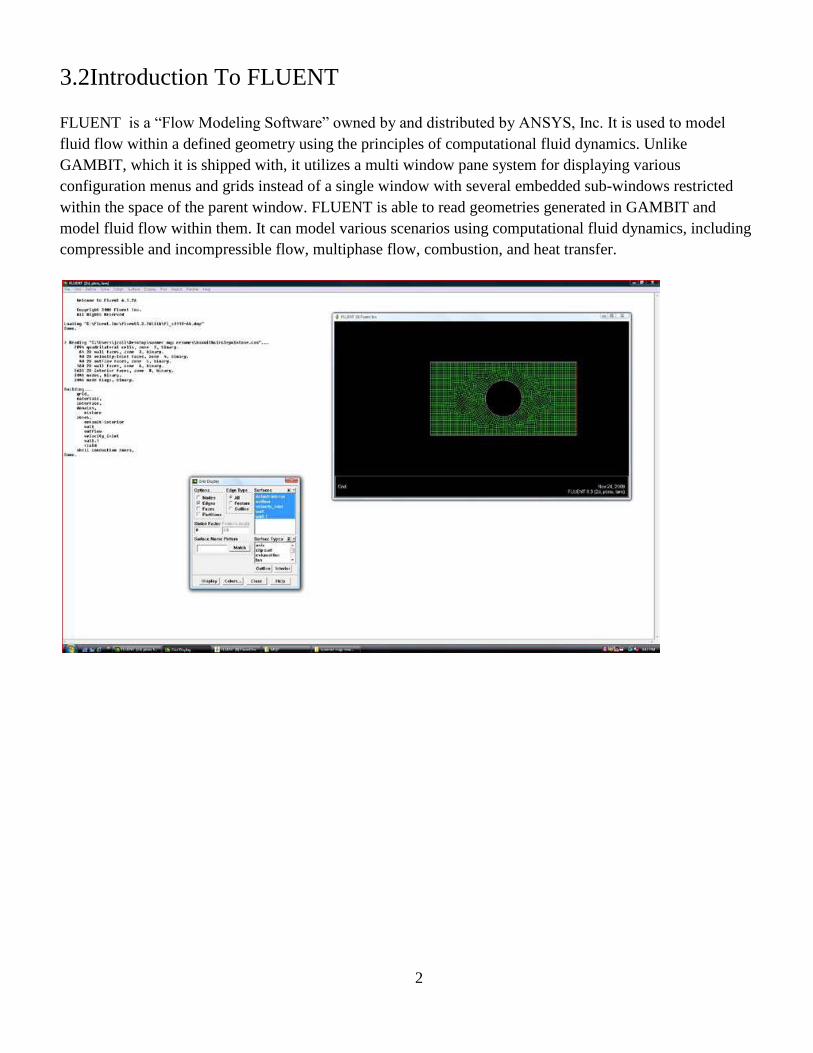
3.2Introduction To FLUENT

FLUENT is a “Flow Modeling Software” owned by and distributed by ANSYS, Inc. It is used to model

fluid flow within a defined geometry using the principles of computational fluid dynamics. Unlike

GAMBIT, which it is shipped with, it utilizes a multi window pane system for displaying various

configuration menus and grids instead of a single window with several embedded sub-windows restricted

within the space of the parent window. FLUENT is able to read geometries generated in GAMBIT and

model fluid flow within them. It can model various scenarios using computational fluid dynamics, including

compressible and incompressible flow, multiphase flow, combustion, and heat transfer.

2

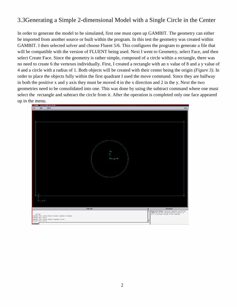
3.3Generating a Simple 2-dimensional Model with a Single Circle in the Center

In order to generate the model to be simulated, first one must open up GAMBIT. The geometry can either

be imported from another source or built within the program. In this test the geometry was created within

GAMBIT. I then selected solver and choose Fluent 5/6. This configures the program to generate a file that

will be compatible with the version of FLUENT being used. Next I went to Geometry, select Face, and then

select Create Face. Since the geometry is rather simple, composed of a circle within a rectangle, there was

no need to create 6 the vertexes individually. First, I created a rectangle with an x value of 8 and a y value of

4 and a circle with a radius of 1. Both objects will be created with their center being the origin (Figure 3). In

order to place the objects fully within the first quadrant I used the move command. Since they are halfway

in both the positive x and y axis they must be moved 4 in the x direction and 2 in the y. Next the two

geometries need to be consolidated into one. This was done by using the subtract command where one must

select the rectangle and subtract the circle from it. After the operation is completed only one face appeared

up in the menu.

2

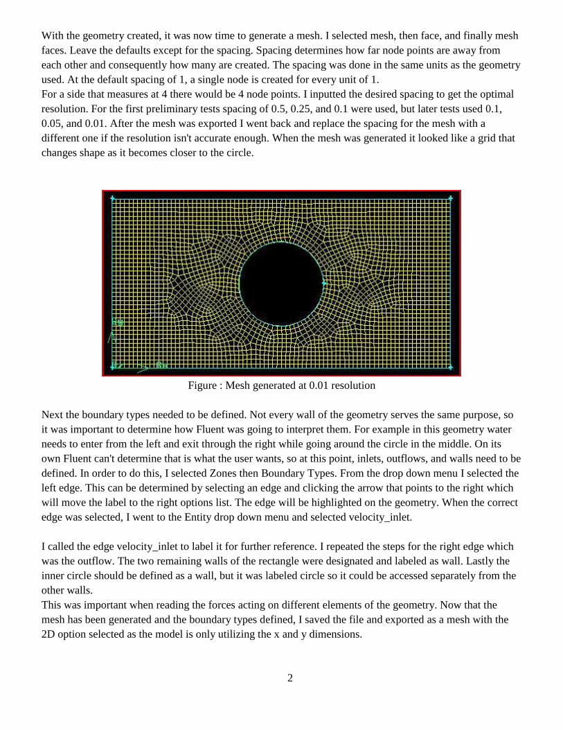
With the geometry created, it was now time to generate a mesh. I selected mesh, then face, and finally mesh

faces. Leave the defaults except for the spacing. Spacing determines how far node points are away from

each other and consequently how many are created. The spacing was done in the same units as the geometry

used. At the default spacing of 1, a single node is created for every unit of 1.

For a side that measures at 4 there would be 4 node points. I inputted the desired spacing to get the optimal

resolution. For the first preliminary tests spacing of 0.5, 0.25, and 0.1 were used, but later tests used 0.1,

0.05, and 0.01. After the mesh was exported I went back and replace the spacing for the mesh with a

different one if the resolution isn't accurate enough. When the mesh was generated it looked like a grid that

changes shape as it becomes closer to the circle.

Figure : Mesh generated at 0.01 resolution

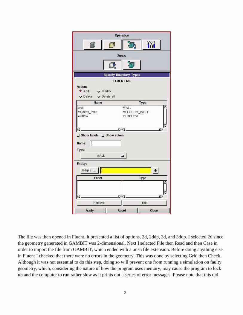
Next the boundary types needed to be defined. Not every wall of the geometry serves the same purpose, so

it was important to determine how Fluent was going to interpret them. For example in this geometry water

needs to enter from the left and exit through the right while going around the circle in the middle. On its

own Fluent can't determine that is what the user wants, so at this point, inlets, outflows, and walls need to be

defined. In order to do this, I selected Zones then Boundary Types. From the drop down menu I selected the

left edge. This can be determined by selecting an edge and clicking the arrow that points to the right which

will move the label to the right options list. The edge will be highlighted on the geometry. When the correct

edge was selected, I went to the Entity drop down menu and selected velocity_inlet.

I called the edge velocity_inlet to label it for further reference. I repeated the steps for the right edge which

was the outflow. The two remaining walls of the rectangle were designated and labeled as wall. Lastly the

inner circle should be defined as a wall, but it was labeled circle so it could be accessed separately from the

other walls.

This was important when reading the forces acting on different elements of the geometry. Now that the

mesh has been generated and the boundary types defined, I saved the file and exported as a mesh with the

2D option selected as the model is only utilizing the x and y dimensions.

2

The file was then opened in Fluent. It presented a list of options, 2d, 2ddp, 3d, and 3ddp. I selected 2d since

the geometry generated in GAMBIT was 2-dimensional. Next I selected File then Read and then Case in

order to import the file from GAMBIT, which ended with a .msh file extension. Before doing anything else

in Fluent I checked that there were no errors in the geometry. This was done by selecting Grid then Check.

Although it was not essential to do this step, doing so will prevent one from running a simulation on faulty

geometry, which, considering the nature of how the program uses memory, may cause the program to lock

up and the computer to run rather slow as it prints out a series of error messages. Please note that this did

2

not catch all possible mistakes. In one test I accidentally labeled the inside circle as the wall where the fluid

outflows.

In this case it did not notify me of the mistake as the program will assume that was intended.

I preceded by selecting Display the Grid. A new configuration window asking for criteria to be determined

opened up but the defaults were all that was needed so I just selected Display. This opened up a new

window displaying the model created in GAMBIT.

2

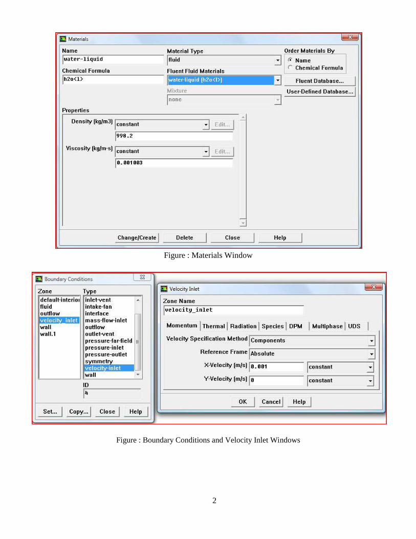
Figure : Materials Window

Figure : Boundary Conditions and Velocity Inlet Windows

2

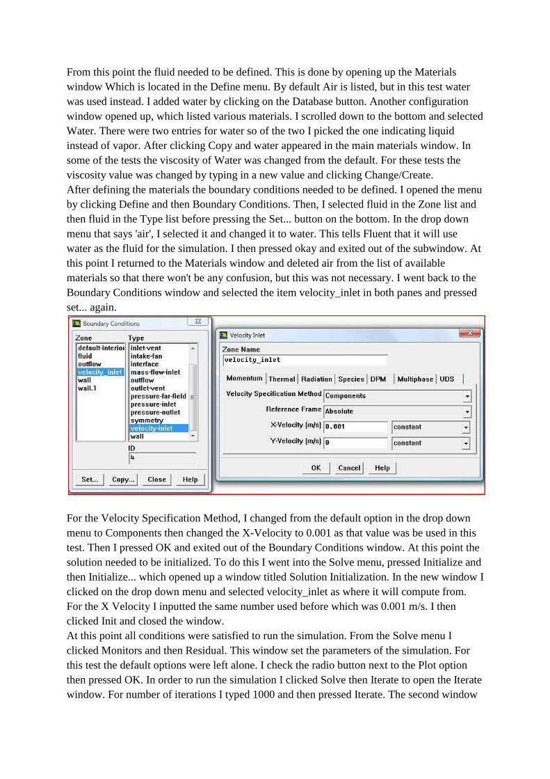
From this point the fluid needed to be defined. This is done by opening up the Materials

window Which is located in the Define menu. By default Air is listed, but in this test water

was used instead. I added water by clicking on the Database button. Another configuration

window opened up, which listed various materials. I scrolled down to the bottom and selected

Water. There were two entries for water so of the two I picked the one indicating liquid

instead of vapor. After clicking Copy and water appeared in the main materials window. In

some of the tests the viscosity of Water was changed from the default. For these tests the

viscosity value was changed by typing in a new value and clicking Change/Create.

After defining the materials the boundary conditions needed to be defined. I opened the menu

by clicking Define and then Boundary Conditions. Then, I selected fluid in the Zone list and

then fluid in the Type list before pressing the Set... button on the bottom. In the drop down

menu that says 'air', I selected it and changed it to water. This tells Fluent that it will use

water as the fluid for the simulation. I then pressed okay and exited out of the subwindow. At

this point I returned to the Materials window and deleted air from the list of available

materials so that there won't be any confusion, but this was not necessary. I went back to the

Boundary Conditions window and selected the item velocity_inlet in both panes and pressed

set... again.

For the Velocity Specification Method, I changed from the default option in the drop down

menu to Components then changed the X-Velocity to 0.001 as that value was be used in this

test. Then I pressed OK and exited out of the Boundary Conditions window. At this point the

solution needed to be initialized. To do this I went into the Solve menu, pressed Initialize and

then Initialize... which opened up a window titled Solution Initialization. In the new window I

clicked on the drop down menu and selected velocity_inlet as where it will compute from.

For the X Velocity I inputted the same number used before which was 0.001 m/s. I then

clicked Init and closed the window.

At this point all conditions were satisfied to run the simulation. From the Solve menu I

clicked Monitors and then Residual. This window set the parameters of the simulation. For

this test the default options were left alone. I check the radio button next to the Plot option

then pressed OK. In order to run the simulation I clicked Solve then Iterate to open the Iterate

window. For number of iterations I typed 1000 and then pressed Iterate. The second window

that displayed the geometry was replaced with a plot with new points being added as time

went. The number of iterations were also be tracked in the main window. Depending on the

resolution running the solution varied in terms of length. In a few circumstances the

simulation may ended before it could finish all 1000

iterations. This meant the solution had converged and the main window indicated that

convergence had been found. In some tests it stopped computing the solution before

convergence was found because the computer ran out of memory to run the operation. In

other tests the solution did not converge after 1000, which prompted me to go back and run

further iterations to see if it converged with more. In the case that they still did not converge,

I compared the earlier solution with the one generated after further iterations. After I

compared the two, I determined whether or not they are close enough to pick a solution.

Since the simulation completed, it was necessary to interpret the results. I did this by clicking

Display, then Contours to open up the Contours configuration window. This displayed the

results of the simulation in contours over the geometry based on the defined parameters that

were being measured. I checked the Filled radio button and then switch the options in the

drop down menus to say Pressure. Clicking Display changed the second plot window into a

contour graph overlaid on top of the geometry. I then checked whether or not the distribution

of pressure forces makes sense using prior knowledge of fluid flow, using the color key on

the right to determine what color means what value. Red represented a higher pressure while

blue indicated low pressure. To see what the actual forces are on specific parts of the

geometry, I clicked Report and then Forces. Under Wall Zone I selected the entries for Wall

and Circle as those are the objects that were being measured in this test. The entry for Force

Vector indicated the direction of the measurement, meaning value of 1 for X and 0 for Y

measured forces in just the x direction. By switching the values and it measured in the y

direction. Since the fluid flow was going horizontally there were minimal forces in the y

direction. I checked the forces in the y direction to verify that was indeed the case. Pressing

Print displayed the pressure, viscous, and total forces for each zone along with the

corresponding coefficients.

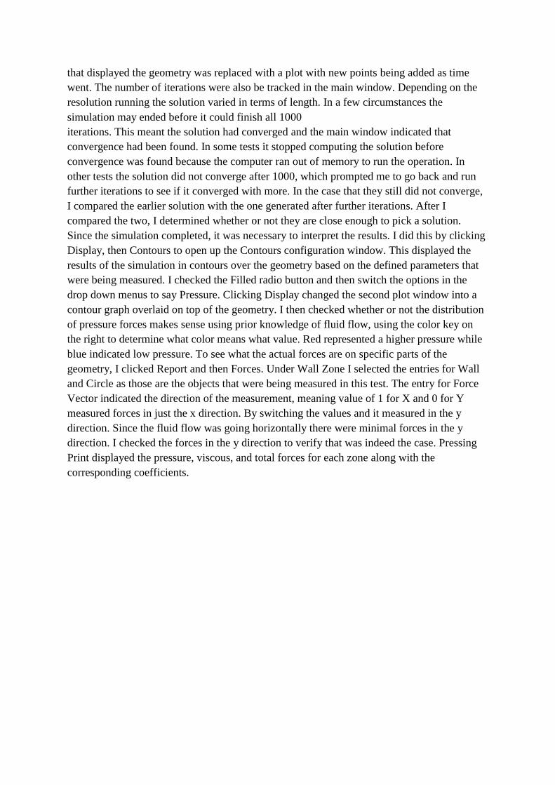
3.4Modelling Of 3D Open Channel Flow :

The Problem is that we have a open Channel whose cross section is 2m in width and 2m in

height and the length of the channel is 6m. There is a obstruction in the mid way of the

channel whose dimensions are 0.5*0.5*2 m.

The Geometry of the open channel is as created in GAMBIT.

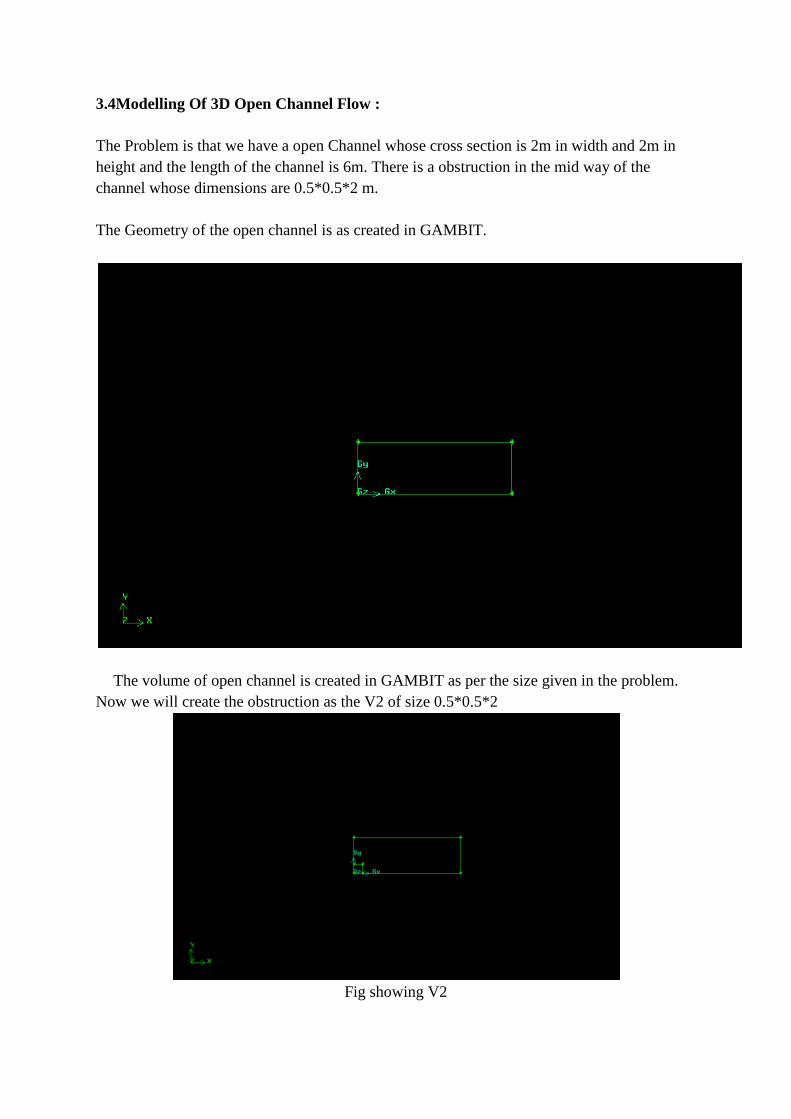
The volume of open channel is created in GAMBIT as per the size given in the problem.

Now we will create the obstruction as the V2 of size 0.5*0.5*2

Fig showing V2

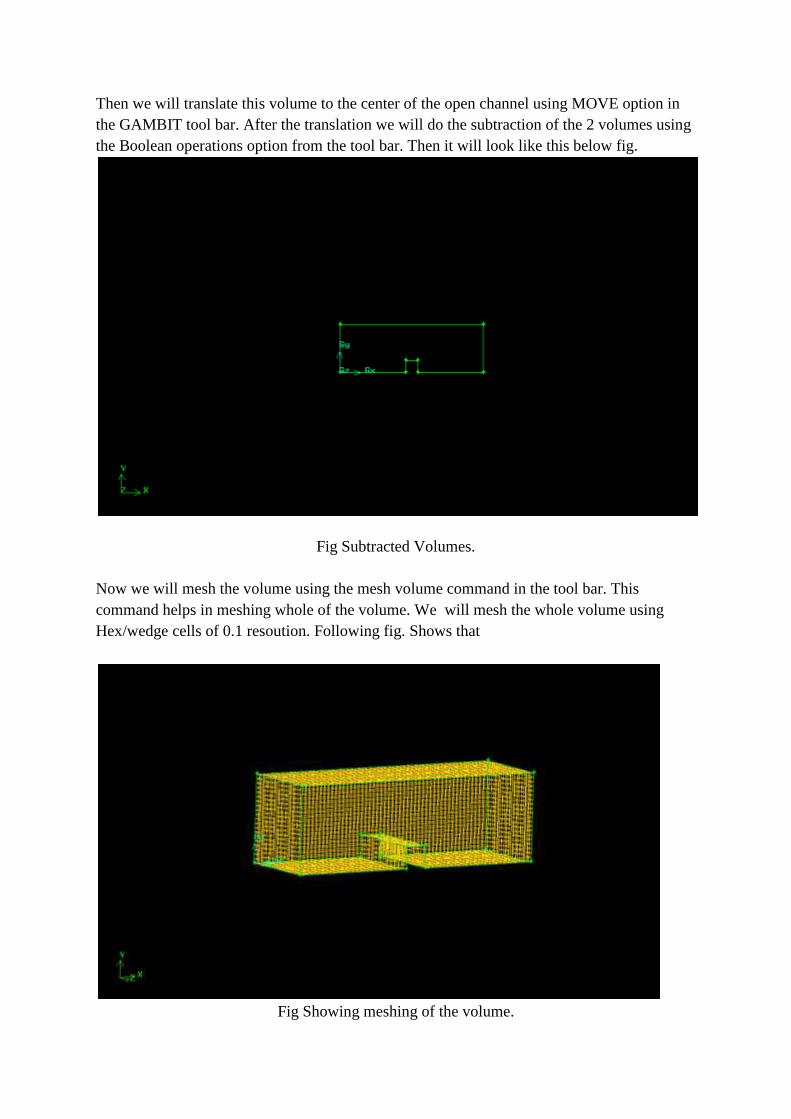
Then we will translate this volume to the center of the open channel using MOVE option in

the GAMBIT tool bar. After the translation we will do the subtraction of the 2 volumes using

the Boolean operations option from the tool bar. Then it will look like this below fig.

Fig Subtracted Volumes.

Now we will mesh the volume using the mesh volume command in the tool bar. This

command helps in meshing whole of the volume. We will mesh the whole volume using

Hex/wedge cells of 0.1 resoution. Following fig. Shows that

Fig Showing meshing of the volume.

Now we will apply boundary conditions over the Face 3 as velocity_inlet and will save the

face as Vin. And Face 4 as the Pressure_outlet and wil save it as PO for our convenience.

Now we will save the file and go to the export option in the file option on the task bar above

and export the mesh so that we can use that mesh for the analysis in FLUENT.

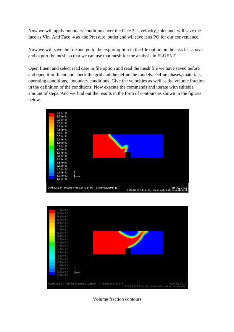
Open fluent and select read case in file option and read the mesh file we have saved before

and open it in fluent and check the grid and the define the models. Define phases, materials,

operating conditions, boundary conditions. Give the velocities as well as the volume fraction

in the definition of the conditions. Now execute the commands and iterate with suitable

amount of steps. And we find out the results in the form of contours as shown in the figures

below.

Volume fraction contours

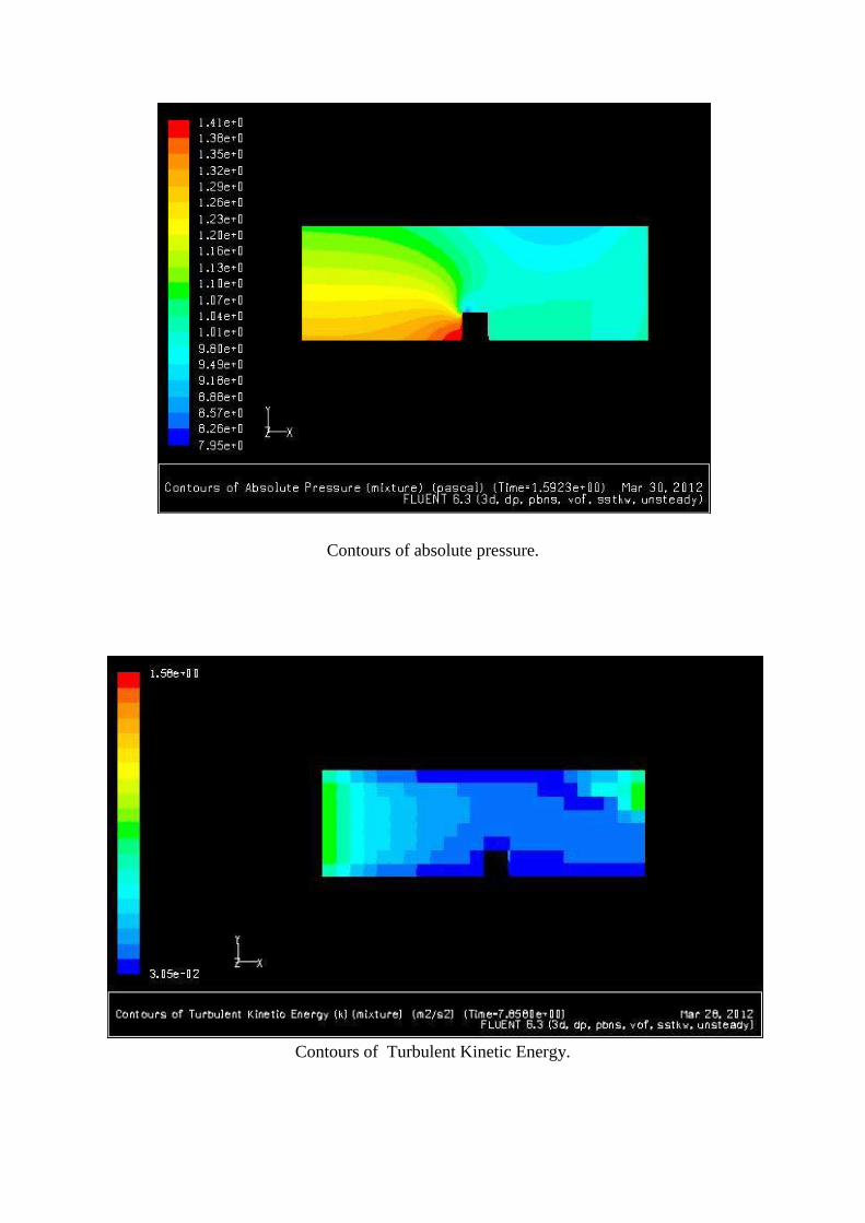
Contours of absolute pressure.

Contours of Turbulent Kinetic Energy.

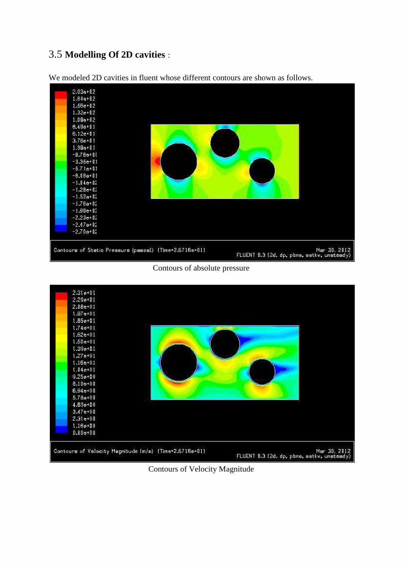
3.5 Modelling Of 2D cavities :

We modeled 2D cavities in fluent whose different contours are shown as follows.

Contours of absolute pressure

Contours of Velocity Magnitude

Contours of turbulent kinetic energy

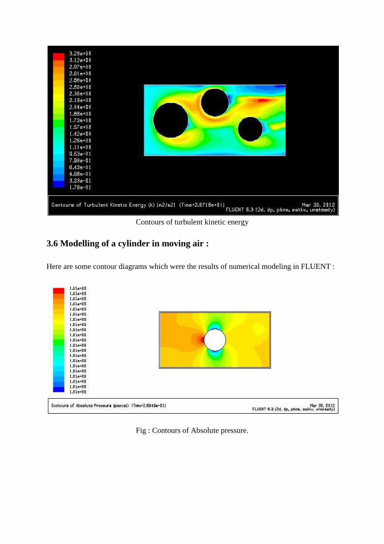
3.6 Modelling of a cylinder in moving air :

Here are some contour diagrams which were the results of numerical modeling in FLUENT :

Fig : Contours of Absolute pressure.

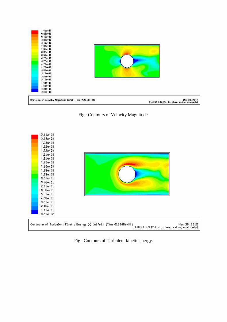
Fig : Contours of Velocity Magnitude.

Fig : Contours of Turbulent kinetic energy.

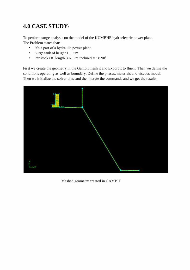
4.0 CASE STUDY:

To perform surge analysis on the model of the KUMBHE hydroelectric power plant.

The Problem states that:

• It’s a part of a hydraulic power plant.

• Surge tank of height 100.5m

• Penstock Of length 392.3 m inclined at 58.90o

First we create the geometry in the Gambit mesh it and Export it to fluent .Then we define the

conditions operating as well as boundary. Define the phases, materials and viscous model.

Then we initialize the solver time and then iterate the commands and we get the results.

Meshed geometry created in GAMBIT

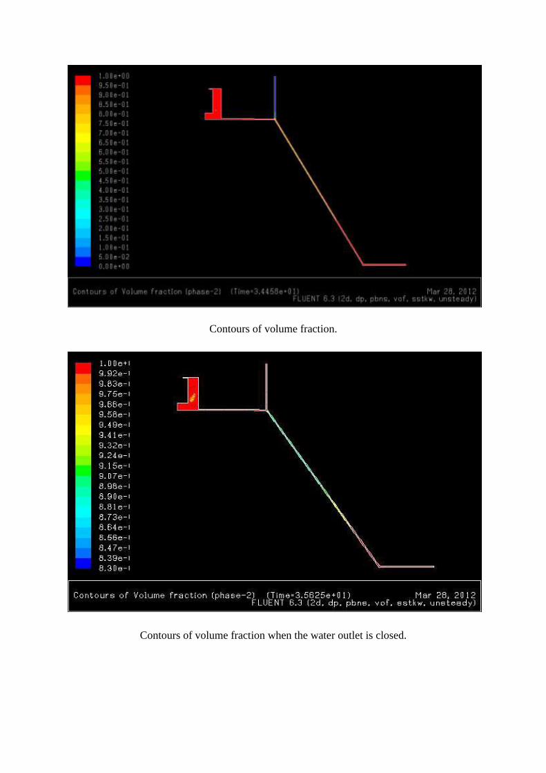
Contours of volume fraction.

Contours of volume fraction when the water outlet is closed.

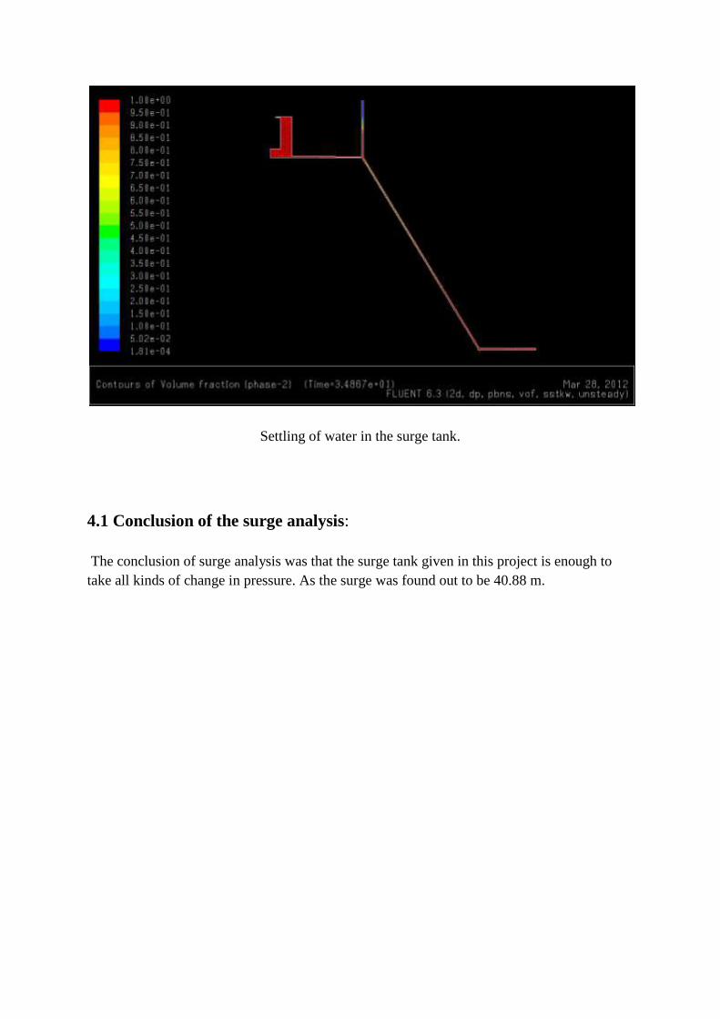
Settling of water in the surge tank.

4.1 Conclusion of the surge analysis:

The conclusion of surge analysis was that the surge tank given in this project is enough to

take all kinds of change in pressure. As the surge was found out to be 40.88 m.

5.0 Conclusion

Computational Fluid Dynamics for all its advances over the past few decades is still nothing

but an approximation and these tests seemed to only reinforce the notion. As the resolution

changes there drag coefficient and overall model changes. Even at a high .01 resolution the

program didn't seem to have settled on a concrete value and one would have reason to believe

that further tests at even higher resolutions would show a change in the model. Furthermore,

due to limitations of computer hardware the higher levels of resolution cannot be computed

without running out of memory. This is especially true considering the simulations run in this

experiment can be considered relatively simple compared to modeling of real life applications

and scenarios. The circumstances may be different if the tests were run in a completely 64 bit

environment, but that was not available for use at the time of conducting the experiment.

If given more time and materials the next logical step would be to devise an experiment with

conditions that can be replicated in both the program and in real life. This would be done

using a wind tunnel or water tank where the fluid flow can be measured along with the forces.

The same conditions would be created in Gambit and simulated in Fluent. In addition, this

would require the 64 bit installation of Fluent on a computer with more than three gigabytes

of random access memory. Only then would one be able to get a good grasp of how accurate

the program is at running simulations.

Eventually it would seem that computational fluid dynamics would advance to the point that

nobody would ever need to conduct actual simulations such as running a wind tunnel.

References

"ANSYS FLUENT Flow Modeling Software." Welcome to ANSYS, Inc. - Corporate

Homepage. Web. 4 Sept. 2009. <http://www.ansys.com/products/fluid-dynamics/fluent/>.

"A Brief History of Computational Fluid Dynamics (CFD) from Fluent." CFD Flow

Modeling Software & Solutions from Fluent. Web. 18 Oct. 2009.

<http://www.fluent.com/about/cfdhistory.htm>.

"Reynolds Number." Engineering ToolBox. Web. 9 Nov. 2009.

<http://www.engineeringtoolbox.com/reynolds-number-d_237.html>.

"Reynolds Number." NASA - Title...Web. 03 Dec. 2009.

<http://www.grc.nasa.gov/WWW/BGH/reynolds.html>. 26

“Computational Fluid Dyanmics” By Anderson.