flow simulation in an ungauged catchment of tonle sap … · flow simulation in an ungauged...

Water Utility Journal 17: 3-17, 2017. © 2017 E.W. Publications

Flow simulation in an ungauged catchment of Tonle Sap Lake Basin in Cambodia: Application of the HEC-HMS model

S. Chea and C. Oeurng* Faculty of Hydrology and Water Resources Engineering, Institute of Technology of Cambodia, Russian Federation Boulevard, P.O. Box 86 Phnom Penh, Cambodia * e-mail: [email protected]

Abstract: Hydrologic modeling is a commonly used tool to estimate water resources availability from ungauged catchments. Several studies have been conducted using HEC-HMS model in different regions under different soil and climatic conditions in order to address issues of land and water use. In this paper, HEC-HMS model is used to simulate rainfall-runoff in Stung Pursat catchment of Tonle Sap Lake Basin in Cambodia. The main objective of this study is to simulate daily stream flow and to assess water availability in catchment following precipitation events. The results showed model performance with NSE, PBIAS and RSR of 0.45, 4.19 and 0.74 for daily simulation, respectively, and 0.61, 10.85 and 0.63 for monthly simulation, respectively. The HEC-HMS conceptual model can be reliably used to simulate flow of Stung Pursat catchment on a continuous time scale, particularly on a monthly basis. The model generated mean annual flow volume in Stung Pursat, Stung Peam and Stung Preykhlong was 743 MCM, 429 MCM and 454 MCM, respectively and the total volume at the outlet at Bac Trakuon station was 1870 MCM per year. Thus, the HEC-HMS model can be considered for flow simulation in other ungauged catchments of the Tonle Sap Lake Basin for the assessment of water availability.

Key words: HEC-HMS, rainfall-runoff, water availability, calibration, simulation

1. INTRODUCTION

Establishing up to date and timely information on the adequacy of available water resources requires a comprehensive assessment strategy (Beven, 2011; Gibbs et al., 2012; Wale et al., 2009). So far, a limited number of catchments have sufficient, continuous hydrologic measurements for comprehensive water resource assessments (Randrianasolo et al., 2011; Wale et al., 2009). A major challenge is the accurate prediction of catchment runoff response to rainfall events (McColl and Aggett, 2007). Researchers have used many methods to assess and predict the intra- and inter-annual availability of water resources within a catchment. Among these methods, decision support tools such as hydrologic models can help researchers to develop better development management strategies for local and regional water resources (Yener et al., 2007).

Hydrologic modeling is a commonly used tool to estimate reach-scale responses to precipitation in catchments under various, riparian management practices (Chu and Steinman, 2009; Kadam, 2011).

The Hydrologic Engineering Centre Hydrologic Modeling System (HEC-HMS) is a commonly used model to simulate rainfall-runoff processes with open source access. Several studies have been conducted using the HEC-HMS model in different regions and under different soil and climatic conditions. For example, (Biswas et al., 2015) uses HEC-HMS to model the effects of climate change and irrigation engineering on the availability of water resources in Bangladesh’s Jamunesswari River. HEC-HMS model was further applied to study effects of urbanization on annual runoff and flood events within the Qinhuai River in Jiangsu Province, P.R. China by coupling distributed hydrologic and dynamic land-use change models (Du et al., 2012). Prediction of both reach-scale and catchment-scale responses to precipitation is particularly important in developing countries such as Bangladesh, China, and Cambodia, where infrastructure, food production, and livelihoods are particularly susceptible to the availability of water resources

4 S. Chea & C. Oeurng

(Kumar and Bhattacharya, 2011; Putty and Prasad, 2000). Water resources within the Pursat River catchment in Cambodia are widely utilized for

irrigation, drinking, and fisheries. However, the sustainability of these water resources within the Pursat River catchment are increasingly under pressure due to dramatic increases in paddy rice production and irrigation, as well as the large scale diversion of water to neighboring catchments for other forms of agriculture (MK16, 2013a). Therefore, understanding and predicting the availability of water resources in this ungauged catchment is importance for management and planning. The objective of this present study is to simulate stream flow, responses to precipitation, and therefore water availability at different spatial scales within this largely ungagged catchment, and evaluate model performance against similar simulations along a gauged reach of the catchment.

2. MATERIALS AND METHODS

2.1 Study area

The Pursat River catchment is located within Pursat Province, south of Tonle Sap Lake (latitude: 12.474243; longitude: 103.50009), and drains an area of 5955 km2. The two main tributaries, the Peam and Santre (Prey Khlong) Rivers, flow in a northerly direction and meet the Pursat River above Bac Trakuon(CNMC, 2011; JICA, 2011). Elevations in the Pursat catchment range between 1 and 1700 masl (Figure 1). More than 75% of the catchment encompasses a hilly terrain, with an elevation greater than 30 masl, and is scattered with forested land of varying densities(JICA, 2011). The remaining low-lying land is used for agriculture. Major soil types in Pursat catchment are dystric leptosol and cambisol in the upper reaches; gleyic and plintic arcsols in the mid-elevation reaches, and; dystric fluvisol and dystric gleysol in the lower elevation reaches (CNMC, 2012). Rainfall within the Pursat River catchment increases with elevation; the annual average rainfall ranges from 1,200 mm to 1,700 mm, but total annual rainfall varies considerably from year to year (JICA, 2013a, b).

Figure 1. Map of Stung Pursat catchment

Water Utility Journal 17 (2017) 5

2.2 Data acquisition

The data being used in this study was obtained from MOWRAM and only climate data was downloaded from global weather data as illustrated in Table 1.

Table 1. Spatial and secondary data

Data type Description Source Topography map Digital Elevation Model (30m x 30m)

Ministry of Water Resources and Meteorology

Land use map Landuse classification (2003) Soil map Soil types (2003) Hydromet data Daily precipitation, Discharge, Water level (2001-2007) Spatial data Basin, sub-basins, river, 3 rainfall and discharge station(s) Climate data Temperature, humidity, etc. (2001-2007) Global weather data

2.3 Catchment delineation

The Pursat River catchment was delineated from the 30m Digital Elevation Model (DEM) obtained from Ministry of Water Resources and Meteorology in order to determine its physical characteristics. The study area was delineated into 43 sub-basins. Each sub-basin’s physical watershed parameters, such as length of flow paths, centroid location, average slope, area, slope and length to the centroid were determined (Gumindoga et al., 2016).

2.4 HEC-HMS hydrological model

HEC-HMS is a hydrologic modeling software package developed by the US Army Corps of Engineers-Hydrologic Engineering Center (HEC). It is a physically based and conceptual semi-distributed model designed to simulate the rainfall-runoff processes in a wide range of geographic areas, from large river basin water supply and flood hydrology to small urban and natural watershed runoff. The software package includes losses, runoff transform, channel routing, canopy, surface, base flow, rainfall-runoff simulation and parameter estimation. HEC-HMS uses separate models to represent each component of the runoff process, including models that compute runoff volume, models of direct runoff, and models of base flow. Each model run combines a basin model, meteorological model and control specifications with run options to obtain results (Choudhari et al., 2014). The detailed description of the model components is described in sections 2.4.1 to 2.4.6.

2.4.1 Canopy method

For the canopy method, a simple canopy is chosen. This method is a simple representation of a plant canopy. All precipitation is intercepted until the storage capacity is filled. Once the storage is filled, all further precipitation falls to the surface or directly to the soil if no representation of the surface is included. The initial condition of the canopy should be specified as the percentage of the canopy storage that is full of water at the beginning of the simulation. Canopy storage represents the maximum amount of water that can be held on leaves before through-fall the surface begins. The amount of storage is specified as an effective depth of water. The crop coefficient is a ration applied to the potential evapotranspiration (computed in the meteorological model) when computing the amount of water to actually extract from the soil (Roy et al., 2013).

2.4.2 Surface method

Surface method use to present the ground surface where water may accumulate in depression storage areas. Net precipitation accumulates in the depression storage areas and infiltrates as the soil has capacity to accept water, thereby reducing the precipitation available for direct flow. Water in


surface interception storage is precipitation not captured by canopy interception and in excess of the infiltration rate. Precipitation is held in surface interception storage until it is removed by infiltration and evapotranspiration (Engineers, 2008).

2.4.3 Runoff method

In Clark Unit Hydrograph transform method, it requires two parameters, time of concentration, Tc and a storage coefficient, R. The Clark unit hydrograph has been applied for estimating direct runoff. Clark’s model derives a watershed UH by explicitly representation to runoff:

§ Translation of the excess from its origin throughout the drainage system to the watershed outlet

§ Attenuation of the magnitude of the discharge as the excess is stored throughout the watershed

Short-term storage of water throughout a watershed in the soil, on the surface, and in the channels plays a crucial role in the transformation of precipitation excess to runoff. The linear reservoir model is a common representation of the effects of this storage.

The time of concentration is defined as the time duration for a drop of water falling in the most remote point of a drainage basin to travel to the outflow point. One of the widely used methods is the SCS lag equation (Roseke, 2013). In metric, the formulas are:

( )S

SLTC 5.0238,4

4.25' 7.08.0

×

+=

(1)

254400,25' −=CN

S (2)

( ) cTSDAR −××= 539.0081.02.142 (3)

in which S’ is the maximum retention, Tc is the time of concentration, L is the flow length (m), CN is the curve number, s is an average watershed land slope (%), DA is a drainage area (km²), S is a channel slope (m/km).

The CN for a watershed can be estimated as a function of landuse, soil type and antecedent watershed moisture as:

∑

∑=

iAiCNiA

compositeCN (4)

in which CNcomposite is the composite CN used for runoff volume; i is an index of watersheds subdivisions of uniform land use and soil type; CNi is the CN for subdivision i; Ai is the drainage area of subdivision i.

2.4.4 Loss method

The soil moisture accounting loss method uses five layers to represent the dynamics of water movement above and in the soil. The layers include canopy interception. Surface depression storage, soil, upper groundwater, and lower groundwater, as shown in Figure 2. Initial conditions for the five storage layers must be specified as the percentage of water in the respective storage layers prior to the start of the simulation. Maximum canopy storage represents the maximum amount of water that can be held on leaves before through fall to surface begins. Surface storage represents the maximum amount of water that can pond on the soil surface before surface runoff


begins. Surface runoff occurs when the storage is at full capacity and there is excess precipitation. The maximum infiltration rate has been specified as the upper limit of the rate of water entry from surface storage into the soil. The percentage of impervious areas was specified as the percentage of the area under urban civilization for each sub-basin. Soil storage was specified as the total storage of water available in the soil profile. Tension storage, another component of the upper soil layer parameter values was derived by determining the field capacity of the soil based on different soil texture (Singh and Jain, 2015).

Figure 2. Soil Moisture Accounting Model (HEC-HMS, 2000)

2.4.5 Routing method

In this study, Muskingum method is chosen for channel routing. X and K parameters must be evaluated. Theoretically, X parameter is constant coefficient that its value varies between 0 - 0.5 and K parameter is time of passing of a wave in reach length and it ranks from 0.1HR to 150HR. Therefore, parameters can be estimated with the help of observed inflow and outflow hydrographs. Parameter K estimated as the interval between similar points on the inflow and outflow hydrographs. Once K is estimated, X can be estimated by trial and error (Engineers, 2008).

2.4.6 Base flow method

The linear-reservoir base flow model is used in conjunction with the continuous soil moisture accounting model. This base flow model simulates the storage and movement of subsurface flow as storage and movement of water through reservoirs. The reservoir is linear the outflow at each time step of the simulation is a linear function of the average storage during the time step. Mathematically, this is identical to the manner in which Clark’s UH model represents watershed


runoff. The outflow from groundwater layer 1 of the SMA is inflow to one linear reservoir, and the

outflow from groundwater layer 2 of the SMA is inflow to another. The outflow from the two linear reservoir is combined to compute the total base flow for the watershed (Engineers, 2008).

2.5 Sensitivity analysis

Some parameters in the method mentioned above is used to do a sensitivity analysis to reduce and save time in calibration periods and identify the most and least sensitive parameter. Thirteen parameters among the twenty-seven parameters was varied an analyzed from -50% to +50% with increment of 10%, keeping all other parameters constant.

2.6 Model calibration

A model is considered plausible only when it can reliably estimate stream flow as compared to observed stream flow. The model was calibrated for the identified sensitive parameters to improve model predictability to achieve good agreement between the simulated and observed data (Choudhari et al., 2014). Optimization trials available in HEC-HMS model have been used for optimizing the initial estimates of the model parameters. For the current study, the Nash-Sutcliffe method was used an objective function with the Univariate Gradient method as the search method for optimization. The auto-calibration process in the HEC-HMS may not converge to desired optimum results, therefore the model was calibrated with both manual and auto-calibration. Generally, manual calibration provides the range of the parameters while the auto-calibration process optimized the result (Singh and Jain, 2015).

2.7 Model evaluation

HEC-HMS model in this study will be assessed using various standard statistical tests of error functions such as Nash-Sutcliff efficiency (NSE), Percentage of Bias (PBIAS) and RMSE-observation standard deviation ratio (RSR).

- Nash-Sutcliff efficiency (NSE)

∑=

⎟⎠⎞⎜⎝

⎛ −

∑=

⎟⎠⎞⎜⎝

⎛ −−=n

iomQ

oiQ

n

ieiQ

oiQ

NASE

1

21

2

1

(5)

- Percentage of Bias (PBIAS)

100×∑

∑ ∑−=

Qoi

QeiQoiPBIAS (6)

- RMSE-observation standard deviation ratio (RSR)

( )

( ) ⎥⎥⎦

⎤

⎢⎢⎣

⎡∑=

−

⎥⎥⎦

⎤

⎢⎢⎣

⎡∑=

−

=n

iQomQoi

n

iQeiQoi

RSR

1

2

1

2

(7)


in which Q!! and Q!! are the estimated and observed discharges (m3 s-1), VolObs and VolOut are the observed and estimated volume, Q!! and Q!! are mean of the estimated and observed discharges (m3 s-1), n is the number of data pairs.

Table 2 is used to determine the range of performance evaluation of HEC-HMS model based on Singh et al. (2005) and Chung et al. (2002).

Table 2. Range of performance evaluation

No Performance Rating NSE RSR PBIAS (%) 1 Very Good 0.75 - Unity 0 - 0.5 <±10 2 Good 0.65 - 0.75 0.5 - 0.6 ±10 - ±15 3 Satisfactory 0.50 - 0.65 0.6 - 0.7 ±15 - ±25 4 Unsatisfactory < 0.50 > 0.7 > ±25

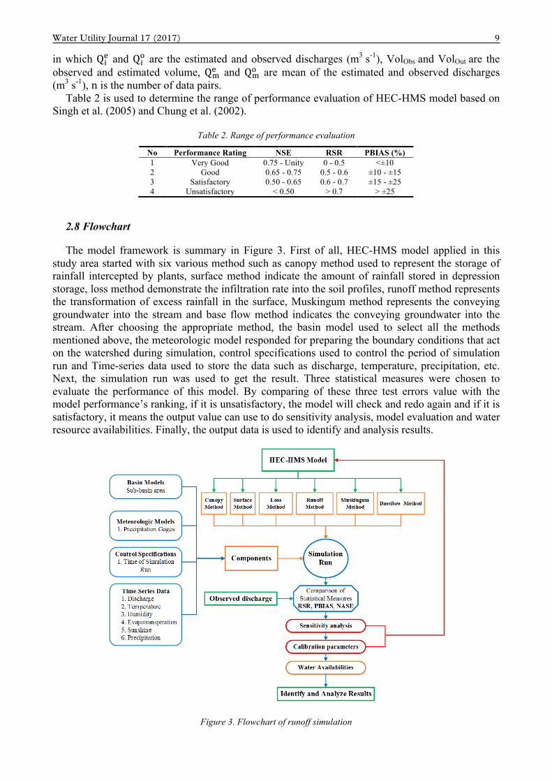
2.8 Flowchart

The model framework is summary in Figure 3. First of all, HEC-HMS model applied in this study area started with six various method such as canopy method used to represent the storage of rainfall intercepted by plants, surface method indicate the amount of rainfall stored in depression storage, loss method demonstrate the infiltration rate into the soil profiles, runoff method represents the transformation of excess rainfall in the surface, Muskingum method represents the conveying groundwater into the stream and base flow method indicates the conveying groundwater into the stream. After choosing the appropriate method, the basin model used to select all the methods mentioned above, the meteorologic model responded for preparing the boundary conditions that act on the watershed during simulation, control specifications used to control the period of simulation run and Time-series data used to store the data such as discharge, temperature, precipitation, etc. Next, the simulation run was used to get the result. Three statistical measures were chosen to evaluate the performance of this model. By comparing of these three test errors value with the model performance’s ranking, if it is unsatisfactory, the model will check and redo again and if it is satisfactory, it means the output value can use to do sensitivity analysis, model evaluation and water resource availabilities. Finally, the output data is used to identify and analysis results.

Figure 3. Flowchart of runoff simulation


3. RESULTS AND DISCUSSION

3.1 Sensitivity analysis

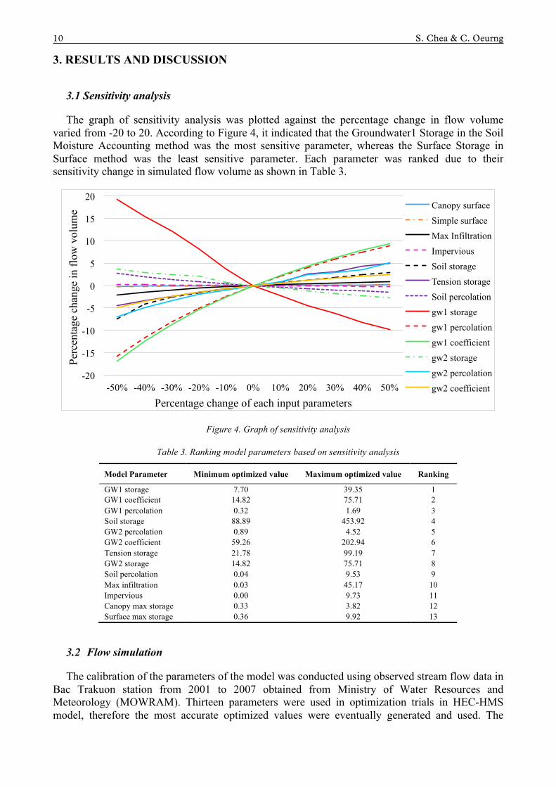
The graph of sensitivity analysis was plotted against the percentage change in flow volume varied from -20 to 20. According to Figure 4, it indicated that the Groundwater1 Storage in the Soil Moisture Accounting method was the most sensitive parameter, whereas the Surface Storage in Surface method was the least sensitive parameter. Each parameter was ranked due to their sensitivity change in simulated flow volume as shown in Table 3.

Figure 4. Graph of sensitivity analysis

Table 3. Ranking model parameters based on sensitivity analysis

Model Parameter Minimum optimized value Maximum optimized value Ranking

GW1 storage 7.70 39.35 1 GW1 coefficient 14.82 75.71 2 GW1 percolation 0.32 1.69 3 Soil storage 88.89 453.92 4 GW2 percolation 0.89 4.52 5 GW2 coefficient 59.26 202.94 6 Tension storage 21.78 99.19 7 GW2 storage 14.82 75.71 8 Soil percolation 0.04 9.53 9 Max infiltration 0.03 45.17 10 Impervious 0.00 9.73 11 Canopy max storage 0.33 3.82 12 Surface max storage 0.36 9.92 13

3.2 Flow simulation

The calibration of the parameters of the model was conducted using observed stream flow data in Bac Trakuon station from 2001 to 2007 obtained from Ministry of Water Resources and Meteorology (MOWRAM). Thirteen parameters were used in optimization trials in HEC-HMS model, therefore the most accurate optimized values were eventually generated and used. The

-20

-15

-10

-5

0

5

10

15

20

-50% -40% -30% -20% -10% 0% 10% 20% 30% 40% 50%

Perc

enta

ge c

hang

e in

flow

vol

ume

Percentage change of each input parameters

Canopy surface Simple surface Max Infiltration Impervious Soil storage Tension storage Soil percolation gw1 storage gw1 percolation gw1 coefficient gw2 storage gw2 percolation gw2 coefficient


comparison of hydrographs representing simulated and observed stream flow during the calibration period of 7 years in shown in Figure 5 and Figure 7.

Figure 5. Comparison of simulated and observed flow during calibration (2001-2007)

The comparison of daily simulation between simulated and observed flow in Figure 5 indicates that the model did not predict the stream flow well yet. From 2001 to 2007, it represents the underestimation for the high flow during the wet season. The error may result from unregulated data observations when flow increased moderately at the beginning of the wet season due to early arrival of rain in May and June. Rain sharply increased from September to October. Moreover, it indicates the overestimation for the low flow in the dry season period. This error may be due to various water diversions for farming by downstream communities in the early dry season, which is not accounted for in the model (Sokhem, 2015).

Regression of daily simulation between simulated and observed flow is shown in Figure 6. The plotted points were above the line 1:1, its represent an overestimation, while below that indicate an underestimation. The most plotted points of simulated and observed discharge are under the line 1:1 which represent the underestimation of model.

Figure 6. Regression between simulated and observed flow for daily simulation


The comparison of monthly simulation between observed and simulated stream flow during the calibration of 7 years period is shown in Figure 7.

Figure 7. Comparison of monthly simulated and observed stream flow during calibration (2001-2007)

This monthly comparison shows a better agreement between observed and simulated stream flow during the last three years (2005-2007), while the first three years (2001-2003) represented an underestimation. These errors may result from the quality of observed flow data, or flows from other, non-point sources. In contrast, an overestimation occurred in 2004. Again, this error may be due to diversion of flow through the irrigation canals. The regression of monthly simulation between simulated and observed flow is shown in Figure 8. This graph represents the improvement of simulated and observed flow.

Figure 8. Correlation of monthly simulation between simulated and observed flow

3.3 Model evaluation

Time-series of simulated and observed flows were taken from the results of simulation run of HEC-HMS model in the Pursat River catchment, and were imported and analyzed in excel to evaluate the model performance both daily and monthly simulation.


The performance evaluation of model based on various standard statistical tests of error functions such as Nash-Sutcliff efficiency (NSE), Percentage of Bias (PBIAS) and RMSE-observation standard deviation ratio (RSR). The value of each standard statistical error is listed in Table 4.

Table 4. Summary of daily and monthly statistical measure values

Daily Simulation Monthly Simulation RSR 0.74 RSR 0.63

PBIAS 4.79% PBIAS 10.85% NASE 0.451 NASE 0.61

3.4 Water resources availability of Stung Pursat catchment

3.4.1 Flow duration curve analysis

A flow duration curve (FDC) represents the relationship between the magnitude and frequency of daily stream flow for a particular river basin, providing an estimate of the percentage of time a given mean streamflow was equaled or exceeded over a historical period (Vogel and Fennessey, 1994). An FDC provides a simple, yet comprehensive, graphical view of the overall historical variability associated with stream flow in a catchment. The shape of the flow duration curve for any river strongly reflects the type of flow regime and is influenced by the characteristics of the upstream catchment including geology, urbanization, artificial influences and groundwater. Therefore, to build the FDC, the flow rates were plotted against the percentile % (percentage exceedance) scale as illustrated in Figure 9. At 20% exceedance, the flow was over 100 m3/s. This is a high flow rate and it indicates the type of flood regime the basin is likely to have, whereas, at 80% exceedance, the flow was under 1 m3/s and represents the ability of the basin to sustain low flows during dry seasons. From 20% to 80% exceedance, it is a flat curve, which indicates that moderate flows are sustained throughout the year due to natural or artificial stream flow regulation, or due to a large groundwater capacity which sustains the base flow to the stream.

Figure 9. Flow duration curve at Stung Pursat catchment outlet (2001-2007)

3.4.2 Monthly water availability

Water availability is one of the most crucial objectives of this research. Understanding water


availability can be useful for the future development and management of water resources programs. The four main junctions in the Pursat River catchment were chosen to assess water availability Figure 10.

Figure 10. Map of four main junctions in Stung Pursat catchment

The chart of average monthly flow in Stung Pursat (Junction 12) is shown in Figure 11. It has the highest volume of 184 MCM in October and lowest volume of 6 MCM in February.

Figure 11. Average monthly flow volume in Stung Pursat (2001-2007)

In Stung Peam (Junction 10) Figure 12, two highest flow volume occurred in September and October with the average monthly flow volume of 103 MCM and 112 MCM, while the lowest one of 1.9 MCM took place in January.

0 20 40 60 80

100 120 140 160 180 200

Jan Feb Mar Apr May Jun Jul Aug Sep Oct Nov Dec

Flow

vol

ume

(MC

M/m

onth

)

Qmean


Figure 12. Average monthly flow volume in Stung Peam (2001-2007)

Figure 13. Average monthly flow volume in Stung Preykhlong (2001-2007)

Figure 14. Average monthly flow volume at the outlet in Bac Trakuon station (2001-2007)

0

20

40

60

80

100

120


Flow

vol

ume

(MC

M/m

onth

)

Qmean

0

20

40

60

80

100

120

140


Flow

vol

ume

(MC

M/m

onth

)

Qmean

0

100

200

300

400

500


Flow

vol

ume

(MC

M/m

onth

)

Qmean


In Stung Preykhlong (Junction 13), the average monthly flow volume increased repeatedly from 37 MCM in June to 124 MCM in October, and went down to 0.5 MCM in late dry season in May.

At the outlet (Junction 1) which was the interception between the three junctions above, the average monthly flow volume increase from 132 MCM to 465 MCM in wet season, and it decreased between 32 MCM to 13 MCM in mid-dry season. Figure 14 shows the graph of average monthly flow volume at the outlet.

The average annual flow volume from 2001 to 2007 in the Pursat, Peam and Preykhlong Rivers were 743 MCM, 429 MCM, and 454 MCM. The outlet at the Bac Trakuon gauging station has the average annual flow volume of 1870 MCM.

4. CONCLUSION

The HEC-HMS conceptual model can be suitably used to simulate flow of the Pursat River catchment on a continuous time scale, particularly on a monthly basis. The model indicates that water availability in the rivers fell from November to April during 2001-2007, but fluctuated in the late dry season and subsequent, early wet season. The maximum flow volume occurred in October. The average annual flow volume in the Pursat, Peam and Preykhlong River was 743 MCM, 429 MCM and 454 MCM, respectively, and a total volume of 1870 MCM per year was recorded by the gauging station in the outlet at Bac Trakuon. Understanding water availability from these three junctions will be useful to water resources managers; especially, in irrigation sector, domestic use and industry. Therefore, the HEC-HMS model can be considered for flow simulation in other ungauged catchments of Tonle Sap Lake Basin.

ACKNOWLEDGEMENTS

We are grateful to the support of Mr. Tom Brauer, U.S Army Corps of Engineers developer, for his advice in choosing methods suitable for this study area and for his thorough explanation by mail of the HEC-HMS model; to MOWRAM, for great support on both hydrologic and spatial data and supporting documents; and to Benjamin Miller, for editing English.

REFERENCES

Beven, K.J., 2001. Rainfall-Runoff Modelling: The Primer. John Wiley & Sons, Lancaster, UK. Biswas, N.K., Paul, M., RezaulHaider, M., 2015. Calibration and Sensitivity Analysis of a Hydrological Model for Jamunesswari

River Basin of Bangladesh. Choudhari, K., Panigrahi, B., Paul, J.C., 2014. Simulation of rainfall-runoff process using HEC-HMS model for Balijore Nala

watershed, Odisha, India. International Journal of Geomatics and Geosciences, 5(2): 253-265. Chu, X., Steinman, A., 2009. Event and continuous hydrologic modeling with HEC-HMS. Journal of Irrigation and Drainage

Engineering, 135(1): 119-124. Chung, S.-W., Gassman, P., Gu, R., Kanwar, R.S., 2002. Evaluation of EPIC for assessing tile flow and nitrogen losses for

alternative agricultural management systems. Transactions of the ASAE, 45(4): 1135. CNMC, 2011. Profile of Sub Area Tonle Sap (SA-9C), Phnom Penh: Mekong River Commission. CNMC, 2012. Profile of the Tonle Sap Sub-area (SA-9C). Basin Development Plan Program, Phnom Penh: CNMC. Du, J. et al., 2012. Assessing the effects of urbanization on annual runoff and flood events using an integrated hydrological modeling

system for Qinhuai River basin, China. Journal of Hydrology, 464: 127-139. Engineers, U.A.C., 2008. Hydrologic modeling system (HEC-HMS) application guide: version 3.1. 0. Institute for Water Resources,

Davis. Gibbs, M.S., Maier, H.R., Dandy, G.C., 2012. A generic framework for regression regionalization in ungauged catchments.

Environmental Modelling & Software, 27: 1-14. Gumindoga, W., Rwasoka, D.T., Nhapi, I., Dube, T., 2016. Ungauged runoff simulation in Upper Manyame Catchment, Zimbabwe:

Applications of the HEC-HMS model. Physics and Chemistry of the Earth, Parts A/B/C. JICA, 2011. Report on Examination of Impact of New Dam Plans on the West Tonle Sap Irrigation Rehabilitation Project in Pursat

River Basin, Phnom Penh: MOWRAM. JICA, 2013a. Brief Progress Report on the Water Balance Examination Study for Pursat and Baribor River basins. MOWRAM. JICA, 2013b. Water Balance Examination Study on Pursat and Baribor River Basins. MOWRAM.


Kadam, 2011. Simulation of rainfall-runoff process using HEC-HMS model for Balijore Nala watershed, Odisha, India. Unpublished P. G Thesis, 5(2): 253-265.

Kumar, D., Bhattacharya, R., 2011. Distributed rainfall runoff modeling. International Journal of Earth Sciences and Engineering, 4(6): 270-275.

McColl, C., Aggett, G., 2007. Land-use forecasting and hydrologic model integration for improved land-use decision support. Journal of environmental management, 84(4): 494-512.

MK16, 2013a. Water Demand Analysis Within the Pursat River Catchment. Mowram/DHRW Consultants. Putty, M., Prasad, R., 2000. Understanding runoff processes using a watershed model—a case study in the Western Ghats in South

India. Journal of Hydrology, 228(3): 215-227. Randrianasolo, A., Ramos, M., Andréassian, V., 2011. Hydrological ensemble forecasting at ungauged basins: using neighbour

catchments for model setup and updating. Advances in Geosciences, 29: 1-11. Roseke, B., 2013. How to calculate time of concentration using the SCS method. Roy, D., Begam, S., Ghosh, S., Jana, S., 2013. Calibration and validation of HEC-HMS model for a river basin in Eastern India.

ARPN Journal of Engineering and Applied Sciences, 8(1): 33-49. Singh, J., Knapp, H.V., Arnold, J., Demissie, M., 2005. Hydrological modeling of the iroquois river watershed using HSPF and

SWAT1. Wiley Online Library. Singh, W.R., Jain, M.K., 2015. Continuous Hydrologic Modeling using Soil Moisture Accounting Algorithm in Vamsadhara River

Basin, India. Journal of Water Resource and Hydrologic Engineering, 4(4): 398-408, doi: 10.5963/JWRHE0404011 Sokhem, S.S.a.P., 2015. Climate Change and Water Governance in Cambodia. Vogel, R.M., Fennessey, N.M., 1994. Flow-duration curves. I: New interpretation and confidence intervals. Journal of Water

Resources Planning and Management, 120(4): 485-504. Wale, A., Rientjes, T., Gieske, A., Getachew, H., 2009. Ungauged catchment contributions to Lake Tana's water balance.

Hydrological processes, 23(26): 3682-3693. Yener, M., Sorman, A., Sorman, A., Sensoy, A., Gezgin, T., 2007. Modeling studies with Hec-Hms and runoff scenarios in Yuvacik

basin, Turkiye. Int. Congr. River Basin Manage, 4: 621-634.

flow simulation in an ungauged catchment of tonle sap … · flow simulation in an ungauged...

Documents