Flow Estimation Only from Image Data, based onPersistent HomologyAnna Suzuki  ( anna.suzuki@tohoku.ac.jp )

Tohoku UniversityMiyuki Miyazawa 

Tohoku UniversityJames Minto 

University of StrathclydeTakeshi Tsuji 

Kyushu UniversityIppei Obayashi 

RIKENYasuaki Hiraoka 

Kyoto UniversityTakatoshi Ito 

Tohoku University

Research Article

Keywords: topological data analysis, persistent homology, physical properties, �ow channels, fracturenetworks

Posted Date: March 29th, 2021

DOI: https://doi.org/10.21203/rs.3.rs-330050/v1

License: This work is licensed under a Creative Commons Attribution 4.0 International License.  Read Full License

1

Flow Estimation Only from Image Data, based on Persistent Homology 1

2

Anna Suzuki1*, Miyuki Miyazawa1, James Minto2, Takeshi Tsuji3,4, Ippei Obayashi5, 3

Yasuaki Hiraoka6 , and Takatoshi Ito1 4

1 Institute of Fluid Science, Tohoku University, Sendai 980-8577, Japan 5 2 Department of Civil & Environmental Engineering, University of Strathclyde, Glasgow, UK 6 3 Department of Earth Resources Engineering, Kyushu University, Fukuoka 819-0385, Japan 7 4 International Institute for Carbon Neutral Energy Research (WPI-I2CNER), Kyushu University, 8 Fukuoka 819-0385, Japan 9 5 Center for Advanced Intelligence Project, RIKEN, Tokyo 103-0027, Japan 10 6 Kyoto University Institute for Advanced Study, ASHBi, Kyoto University, Kyoto 606-8501, Japan 11

12 *corresponding author(s): Anna Suzuki (anna.suzuki@tohoku.ac.jp) 13

14 15

Abstract (147 words) 16 Topological data analysis is an emerging concept of data analysis for characterizing shapes. A 17

state-of-the-art tool in topological data analysis is persistent homology, which is expected to 18

summarize quantified topological and geometric features. Although persistent homology is 19

useful for revealing the topological and geometric information, it is difficult to interpret the 20

parameters of persistent homology themselves and difficult to directly relate the parameters to 21

physical properties. In this study, we focus on connectivity and apertures of flow channels 22

detected from persistent homology analysis. We propose a method to estimate permeability in 23

fracture networks from parameters of persistent homology. Synthetic 3D fracture network 24

patterns and their direct flow simulations are used for the validation. The results suggest that 25

the persistent homology can estimate fluid flow in fracture network based on the image data. 26

This method can easily derive the flow phenomena based on the information of the structure. 27

28

Introduction 29 Fluid flow processes are ubiquitous in the world, and most are governed by the 30

geometry and nature of the surrounding structures. In particular, recent miniaturization of 31

artificial devices has led to the need for understanding and controlling flow in finer structures. 32

It is also attracting attention to understand flow behaviors in complex fracture networks in 33

developments of natural resources, as in the case of shale gas and geothermal developments. 34

It has been a long-term scientific challenge to predict flow behavior of porous media 35

from structural properties. Permeability is a key parameter for examining flow phenomena in 36

porous media1. Permeability cannot be determined only from structure data, and needs to be 37

obtained from laboratory experiments or numerical fluid flow simulations. In contrast, porosity 38

is a parameter that is often used to characterize the structures. The porosity-permeability 39

correlation has been studied extensively in the literature to estimate permeability using porosity 40

(so-called Kozeny-Carman equation)2,3. This Kozeny-Carman equation provides a relationship 41

between structure and flow. The correlation has been studied extensively in the literature to 42

estimate permeability using porosity. However, no matter how much void there are, if they are 43

not connected, water cannot flow. Therefore, the Kozeny-Carman equation does not always 44

work. The correlation has been modified to represent real phenomena by adding parameters 45

such as fractal dimension, and tortuosity2. These additional parameters can only be determined 46

by fitting, which is not the best way to go about flow prediction based on structural information. 47

Let us also consider flow in a channel from an inlet to an outlet. Hagen-Poiseuille 48

equation is a physical law that describe a steady laminar flow of a viscous, incompressible, and 49

Newtonian fluid through a circular tube of constant radius, r. This is an exact solution for the 50

2

flow, can be derived from the (Navier-) Stokes equations, and is another way of expressing the 51

relationship between structure and flow. Using Darcy’s law, a representative permeability, 𝐾HP 52

[m2], for the capillary can be calculated depending only on the radius: 53

54

𝐾!" =#!

$ (1)55

56

57

Similarly, for flow in a fracture bounded by two smooth, parallel walls, the permeability, 𝐾CL 58

[m2], can be calculated depending only on the aperture, h [m]: 59

60

𝐾%& ='!

() (2) 61

62

Since the flow rate is proportional to the cube of the fracture aperture, this relationship between 63

flow and aperture is well-known as the “cubic law” 4–7. 64

Eqs. (1) and (2) are only ways to obtain simplified analytic solution to describe the 65

relationship between the flow and structures. This is another way to predict permeability from 66

structural properties8. In natural rocks, it is not always a single fracture, but multiple fractures 67

that form a network. Thus, it is necessary to understand not just an individual fracture, but how 68

channels are connected from an inlet to an outlet in whole networks. There have been many 69

studies focusing on networks, but most of the parameters used to describe the structure are 70

probabilistic variables that capture individual fractures, and no suitable parameters have been 71

found yet to evaluate the flow of the entire networks9. 72

Topology, a branch of modern mathematics, is good at roughly investigating the 73

connectivity of shapes. Topology focuses on the properties (called topological properties or 74

topological invariants) that are preserved when some form (shape or space) is continuously 75

deformed (stretched or bent, but not cut or pasted). Topology can extract global features that 76

are difficult to capture with machine learning and convolutional neural networks, so it is 77

promising as a complementary feature to extract image information that cannot be detected 78

with other methods. It can be applied to volumetric data as well, so it can pick up information 79

that has been missed in one-way slice-by-slice analysis common to many forms of data 80

processing. 81

Several studies used topological invariants to describe pore-scale structures in porous 82

materials and fracture networks10,11. The Minkowski functionals can be interpreted as area, 83

perimeter, or the Euler characteristic, which is a topological constant and were used to link to 84

hydraulic properties12,13. Scholz et al. (2012)14 showed an empirical expression of permeability 85

with the Minkowski functionals Liu et al. (2017)15 showed the correlation of relative 86

permeability to one of the topological invariants called Euler characteristic. Armstrong et al. 87

(2019)16 reviewed the theoretical basis of the Minkowski functionals and its application to 88

characterize porous media. Counting the number of holes using topological invariants like they 89

did is a clue to the shape of the object, and the "essential information" can be extracted well. 90

On the other hand, topology too narrowly focuses on the essential information, it also discards 91

a lot of information, such as size of pore space. The size information, such as radii of tube or 92

apertures of fractures in Eqs. (1) and (2), must be detected to determine permeability derived 93

analytically. Therefore, previous studies had to add the size information in other ways. 94

Homology is a standard technique for identifying a topological space. In particular, the 95

concept of homology has traditionally played a role in feature extraction focusing on the 96

existence of “holes”. Here, the “hole” structure can be regarded as a connected flow channels 97

from an inlet to an outlet. It is expected that topology can be used to detect such connected 98

flow channels. 99

3

By tracking the sequence of topological spaces, namely, by recording how long 100

homological features persist, we can add information about the size and length of the holes. 101

This can give us a quantitative indication of the size of the holes and the amount of space 102

available, which is called persistent homology. Persistent homology is one of the most 103

important tools in topological data analysis and is expected to compute geometric and 104

topological features of various shapes with ease of computation17–20. Thus, this has been 105

applied in several research fields21–25, and is also beginning to be used in the analysis of porous 106

materials26–31. 107

At this point, in contrast to topological invariants, persistent homology can provide a 108

lot of information that we might need, but it is difficult to interpret the parameters of persistent 109

homology themselves27–30. Ushizima et al. (2012)26 estimates permeability of porous rocks by 110

using Reeb graphs to represent the pore networks. They use persistent homology to distinguish 111

between significant and “noisy” pore spaces, and to supplement the Reeb graphs. Their paper 112

did not go into quantitative evaluation, but focused on qualitative evaluation and visualization. 113

As mentioned before, the “hole” structure that is characterized by topology, can be regarded as 114

connected flow channels from an inlet to an outlet. The aim of our study is to detect the flow 115

channels by persistent homology. Suzuki et al. (2020)31 proposes a method to detect flow 116

channels in 2D images from persistent homology through image processing. By using their 117

image processing procedure, persistent homology is expected to detect such connected flow 118

channels in complex fracture networks and would also provide their size information such as 119

apertures to predict the permeability. 120

In this study, we applied persistent homology to estimate permeability in fracture 121

networks based on image data. Persistent homology was used to detect the number of flow 122

channels and their apertures in the networks. Synthetic fracture networks were generated, and 123

direct flow simulation was conducted. Permeability derived from persistent homology and 124

simulation results were compared. We applied the proposed method to several published image 125

data and discussed the applicability of permeability estimation based on persistent homology. 126

127

Results 128

Detection of flow channels from persistent homology analysis 129

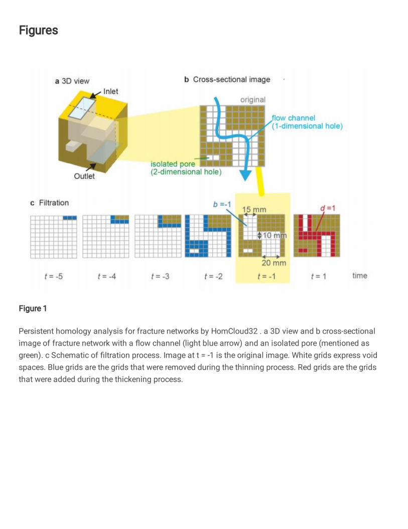
An example of a fractured rock model with a flow channel connecting an inlet to an 130

outlet is shown in Figure 1a. The yellow area is a solid skeleton, while the white area is 131

fractures forming void spaces. The connecting fractures from the top (inlet) to the bottom 132

(outlet) can be a flow channel. In persistent homology analysis, such structure is recognized as 133

“hole” and quantified as a 1-dimensional hole. Additionally, a discrete island (i.e., connected 134

component) is quantified as a 0-dimensional hole, and a ball (i.e., enclosed solid voids) is 135

quantified as a 2-dimensional hole. The numbers of k-dimensional holes (the dimension of the 136

kth homology vector space) are known to the kth Betti number (β0, β1, and β2). This study 137

focuses on “hole” structures penetrating from an inlet to an outlet, which can be flow channels 138

hence we only analyze 1-dimensional holes in this study. 139

One aspect of persistent homology analysis is that independent fractures are recognized 140

as 2-dimensional holes, as shown in Figure 1b. These independent fractures would not 141

contribute to the fluid flow. Therefore, we can distinguish fractures that act as flow channels 142

and independent fractures by 1-dimensional holes and 2-dimensional holes. 143

144

4

145 Figure 1 | Persistent homology analysis for fracture networks by HomCloud32. a 146

3D view and b cross-sectional image of fracture network with a flow channel (light blue 147

arrow) and an isolated pore (mentioned as green). c Schematic of filtration process. 148

Image at t = -1 is the original image. White grids express void spaces. Blue grids are 149

the grids that were removed during the thinning process. Red grids are the grids that 150

were added during the thickening process. 151

152 Much research has explored various applications of persistent homology in statistical 153

data analysis of point cloud data22,33,34. Since the purpose of this study is to analyze the 154

information of structures based on the image data (e.g., micro-CT images), binarized digital 155

images were used for analysis. Jiang et al. (2018)29 applied persistent homology to analyzed 156

rock pore geometries obtained from micro-CT images. The rock pore geometries were first 157

represented as sphere cloud data using a pore-network extraction method, then analyzed 158

by calculating the Vietoris-Rips complex topology of the input sphere cloud data. We used an 159

open software HomCloud (https://homcloud.dev/) to analyze binarized 3D images, which can 160

obtain the information of persistent homology by calculating the Euclidian distance of 2D or 161

3D black and white images32. 162

Figure 1c shows an example of data process in our persistent homology analysis, 163

called filtration17. In filtration, the solid skeletons (yellow parts) are made thinner or thicker, 164

voxel-by-voxel. The original image is set to -1. The process of thinning yellow voxels adjacent 165

to white voxels is regarded as -1, while the process of thickening yellow voxels adjacent to 166

white voxels is regarded as +1. When we reduce the time, the space eventually becomes empty. 167

The nested sequence of the topological spaces from the empty space to the filled space is 168

recorded. The times when the hole appears or disappears are called “birth time” or “death time”, 169

expressed as “b”. or “d”, respectively. 170

In filtration (Figure 1c), a point of the flow channel is closed at t = 1. This closed point 171

is the narrowest aperture in the flow channel. Taking advantage of this, the length of narrowest 172

aperture can be obtained as death time d multiplied by two and its resolution δ. (narrowest 173

5

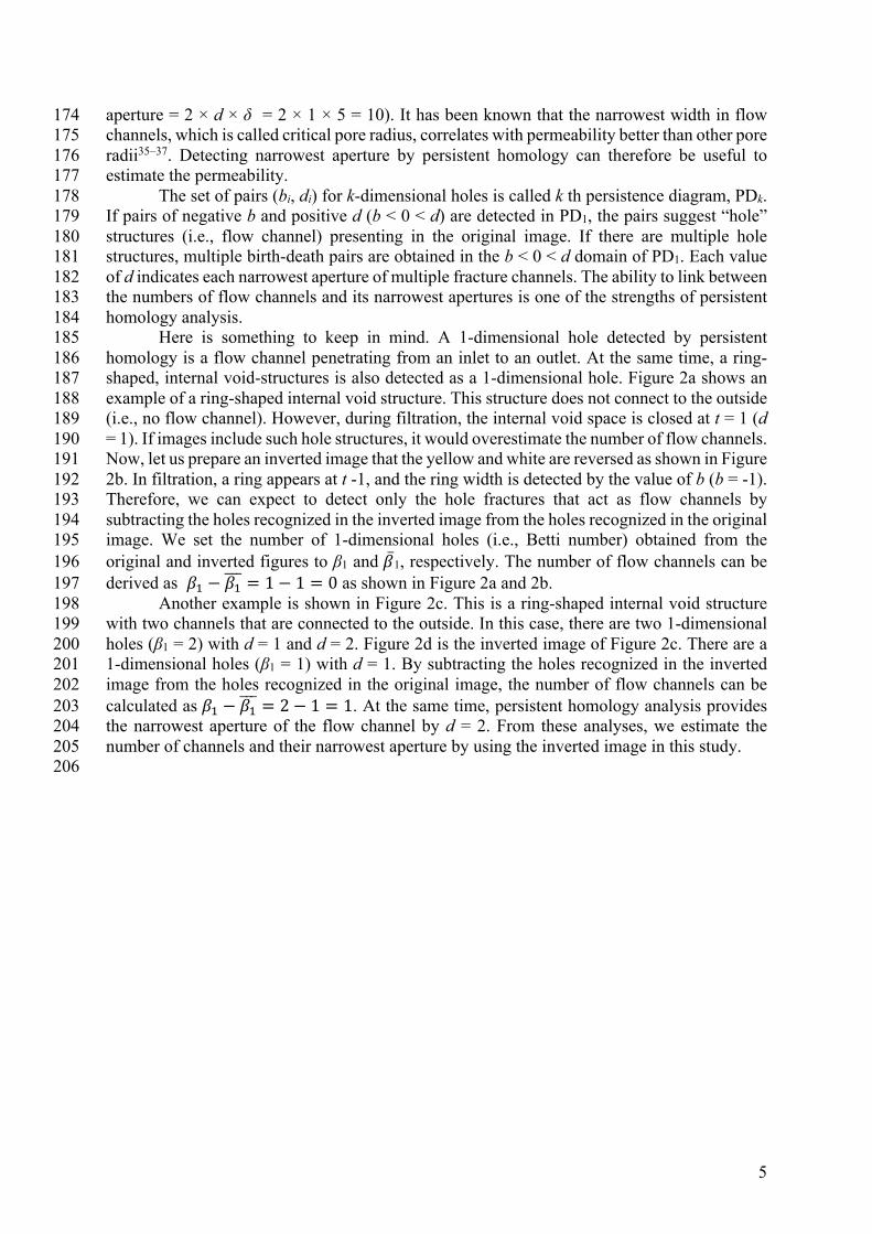
aperture = 2 × d × δ = 2 × 1 × 5 = 10). It has been known that the narrowest width in flow 174

channels, which is called critical pore radius, correlates with permeability better than other pore 175

radii35–37. Detecting narrowest aperture by persistent homology can therefore be useful to 176

estimate the permeability. 177

The set of pairs (bi, di) for k-dimensional holes is called k th persistence diagram, PDk. 178

If pairs of negative b and positive d (b < 0 < d) are detected in PD1, the pairs suggest “hole” 179

structures (i.e., flow channel) presenting in the original image. If there are multiple hole 180

structures, multiple birth-death pairs are obtained in the b < 0 < d domain of PD1. Each value 181

of d indicates each narrowest aperture of multiple fracture channels. The ability to link between 182

the numbers of flow channels and its narrowest apertures is one of the strengths of persistent 183

homology analysis. 184

Here is something to keep in mind. A 1-dimensional hole detected by persistent 185

homology is a flow channel penetrating from an inlet to an outlet. At the same time, a ring-186

shaped, internal void-structures is also detected as a 1-dimensional hole. Figure 2a shows an 187

example of a ring-shaped internal void structure. This structure does not connect to the outside 188

(i.e., no flow channel). However, during filtration, the internal void space is closed at t = 1 (d 189

= 1). If images include such hole structures, it would overestimate the number of flow channels. 190

Now, let us prepare an inverted image that the yellow and white are reversed as shown in Figure 191

2b. In filtration, a ring appears at t -1, and the ring width is detected by the value of b (b = -1). 192

Therefore, we can expect to detect only the hole fractures that act as flow channels by 193

subtracting the holes recognized in the inverted image from the holes recognized in the original 194

image. We set the number of 1-dimensional holes (i.e., Betti number) obtained from the 195

original and inverted figures to β1 and �̅�1, respectively. The number of flow channels can be 196

derived as 𝛽! − 𝛽!&&& = 1 − 1 = 0 as shown in Figure 2a and 2b. 197

Another example is shown in Figure 2c. This is a ring-shaped internal void structure 198

with two channels that are connected to the outside. In this case, there are two 1-dimensional 199

holes (β1 = 2) with d = 1 and d = 2. Figure 2d is the inverted image of Figure 2c. There are a 200

1-dimensional holes (β1 = 1) with d = 1. By subtracting the holes recognized in the inverted 201

image from the holes recognized in the original image, the number of flow channels can be 202

calculated as 𝛽! − 𝛽!&&& = 2 − 1 = 1. At the same time, persistent homology analysis provides 203

the narrowest aperture of the flow channel by d = 2. From these analyses, we estimate the 204

number of channels and their narrowest aperture by using the inverted image in this study. 205

206

6

. 207

Figure 2 | Detecting flow channels using inverted images a ring-shaped, internal 208

void-structure that is not connected to the outside, and b its inverted image. c ring-209

shaped, internal void-structure with two channels that is connected to the outside and 210

forms a flow channel. d its inverted image. The left column shows 3D view of images. 211

The center column describes processes of filtration. The right column lists Betti 212

numbers 𝛽!. 213

214

7

Synthetic fracture network 215 Synthetic fracture networks were generated by using OpenSCAD 216

(https://www.openscad.org/). We distributed multiple penny-shaped fractures by controlling 217

the apertures, radii, numbers, and orientations of fractures to generate a fracture network38. By 218

hollowing out the generated fracture network from a rectangular block, a fractured model 219

where the void spaces were composed of the fracture network was created. This study 220

characterizes one-dimensional flow. The top surface was an inlet, and the bottom surface was 221

an outlet. The fractures were connected from the top to the bottom surfaces. The side 222

boundaries were closed, and water did not flow out from the side. 223

The fractured model is shown in Figure 3. Figure 3a and 3b are the outside and the 224

inside of the model. The fracture orientation was either orthogonal or random. The orthogonal 225

models distributed perpendicular or horizontal fractures to the flow direction (Figure 3c), while 226

the random models distributed fractures by random numbers (Figure 3d). We prepared nine 227

orthogonal models and seven random models. The model parameters for each model are listed 228

in Table 1. 229

230 Figure 3 | Fractured models. a outside and b inside of model. c Orthogonal 231

distribution and d random distribution of fracture networks. 232

233

8

Table 1 | Fracture network parameters and results of permeability. 234

235 Fracture network parameters

Model Diameter

(mm) Aperture

(mm)

Fracture

density parameter

Number

of fractures

Simulation result

PH estimation

Orthogonal

O1 10 0.2 3000 77 1.04 × 10-10 2.47 × 10-10 O2 10 0.6 3000 77 3.03 × 10-9 3.43 × 10-9 O3 10 1.0 3000 77 1.31 × 10-8 1.55 × 10-8

O4 5 0.2-1 6100 234 1.58 × 10-10 2.68 × 10-10 O5 10 0.2-1 1720 66 4.00 × 10-10 7.18 × 10-10 O6 5 0.2-1 2020 251 3.50 × 10-10 2.70 × 10-10

O7 5 0.2-1 13000 230 1.12 × 10-10 2.16 × 10-10 O8 5-25 0.2-1 895 73 3.15 × 10-9 2.20 × 10-9

Random

R1 10 0.2 2000 77 1.01 × 10-10 2.36 × 10-10 R2 10 0.6 2000 77 2.90 × 10-9 3.46 × 10-9 R3 10 1.0 2000 77 1.28 × 10-8 1.39 × 10-8

R4 10 0.2 1000 38 3.42 × 10-11 1.12 × 10-10 R5 10 0.2 3000 115 1.75 × 10-10 3.70 × 10-10 R6 25 1.0 280 11 5.21 × 10-9 4.03 × 10-9

R7 5 0.2 11950 459 1.30 × 10-10 1.36 × 10-10

236

Estimation of fracture numbers and apertures by persistent homology 237 3D image data of each fractured model (36 mm × 36 mm × 50 mm with a voxel 238

resolution δ of 0.1 mm) were binarized and analyzed by persistent homology using 239

HomCloud32. The image size was 360 × 360 × 500 voxels. 240

The estimated narrowest fracture apertures based on the persistent homology analysis 241

are shown in Figure 4. Fracture networks (O1-O3, R1-R3) distributes a single value of fracture 242

aperture of 0.2 mm, 0.6 mm, and 1.0 mm, respectively. Figures 4a and Figure 4b shows the 243

results for the orthogonal and the random fracture networks, respectively. As mentioned before, 244

the narrowest apertures in each flow channel were calculated as 2di δ in persistent homology 245

analysis. The values given in each network (0.2 mm, 0.6 mm, 1.0 mm) are compared with the 246

estimated narrowest apertures (2di δ). The sizes of the circles represent the number of birth-247

death pairs with di. As shown in Figure 4, the estimated narrowest apertures are equal or 248

relatively larger than the actual values given in the network. Most of results are between one 249

or two times larger than the actual values. Persistent homology analysis detects not fractures 250

themselves but flow channels. 251

252 Figure 4 I Estimation of fracture apertures by persistent homology (PH) analysis. 253

a orthogonal fracture networks and b random fracture networks. 254

9

255

Derivation of permeability 256

We use Eq. (2) to derive permeability, which can be originally calculated by comparing 257

the Stokes equation with the Darcy’s law. If Assuming that a fracture is a smooth and parallel 258

plate with the aperture of h and that there is a uniform pressure gradient in one direction within 259

the plane of the fracture, the total volumetric flowrate in the fracture can be written as 260

261

𝑄" = −#$!

!%&

'(

'" (3) 262

263

where w is the width of the fracture, perpendicular to the flow direction. h is the aperture, and 264

μ is the water viscosity, dP/dx is the pressure gradient. Darcy's law describes one-dimensional 265

fluid flow through porous media as 266

267

𝑄" = −)*

&

'(

'" (4) 268

269

where A is the cross-sectional area. Comparison of Eqs. (3) and (4) shows that the permeability 270

of the fracture can be identified as 271

272

𝐾 = −#$!

!%* (5) 273

274

If the cross-sectional areas of the inlet and outlet are assumed to be wh, Eq. (5) becomes Eq. 275

(2). If we consider the case of parallel multiple channels, the permeability can be derived in 276

the following equation 277

278

𝐾 = ∑#"$"

!

!%*

+,-! (6) 279

280

where A is the surface area of the cross section of the medium, and N is the number of flow 281

channels. wi is the depth of flow channel, and hi is the aperture of the flow channel i, i =1,.., N. 282

There is an unknown parameter wi in Eq. (6). The 3D voxel data can be regarded as a series of 283

2D cross-sectional images. The 2D cross-sectional image data provides total area of pore space, 284

Ap in each layer. If we introduce effective depth 𝑤. that is the same for all flow channels, 𝑤. 285

can be derived by 𝑤. =./0(*#)

∑ $"$"%&

where min(𝐴5) is the minimum of total area of pore space 286

for all layers. The number of flow channels N was estimated from the number of birth-death 287

pairs, and the aperture hi was estimated as 2di δ in persistent homology analysis. Thus, Eq. (6) 288

can be written as follows 289

𝐾 =#6

!%*∑ (2𝑑,𝛿)

7+,-! (7) 290

291

Estimation of permeability from persistent homology analysis 292

Before applying complex fracture networks, we validated Eq. (7) and our simulation 293

with simple fracture models. Simple models with one or two fractures penetrating from an 294

inlet to an outlet were used (see Figure 5a). Apertures and number of fractures in each model 295

are listed in Table 2. Direct flow simulation with the same fracture network was conducted in 296

OpenFOAM (https://www.openfoam.com/). We could obtain volumetric flow rate and 297

pressure gradient between the inlet and the outlet to calculate equivalent permeability based on 298

Darcy’s law. Comparison of permeability between flow simulation and persistent homology 299

analysis is shown in Figure 5b, and listed in Table 2. The persistent homology estimation is in 300

10

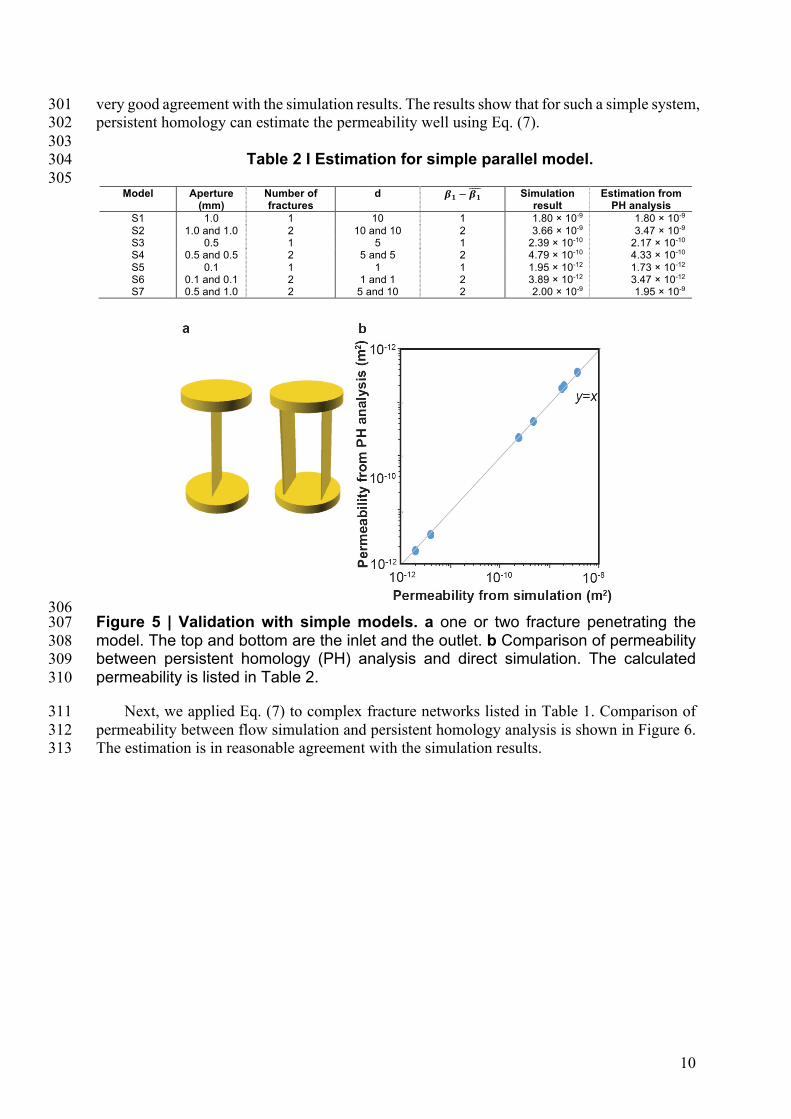
very good agreement with the simulation results. The results show that for such a simple system, 301

persistent homology can estimate the permeability well using Eq. (7). 302

303

Table 2 I Estimation for simple parallel model. 304

305 Model Aperture

(mm) Number of fractures

d 𝜷𝟏 − 𝜷𝟏#### Simulation

result Estimation from

PH analysis

S1 1.0 1 10 1 1.80 × 10-9 1.80 × 10-9

S2 1.0 and 1.0 2 10 and 10 2 3.66 × 10-9 3.47 × 10-9 S3 0.5 1 5 1 2.39 × 10-10 2.17 × 10-10 S4 0.5 and 0.5 2 5 and 5 2 4.79 × 10-10 4.33 × 10-10

S5 0.1 1 1 1 1.95 × 10-12 1.73 × 10-12 S6 0.1 and 0.1 2 1 and 1 2 3.89 × 10-12 3.47 × 10-12 S7 0.5 and 1.0 2 5 and 10 2 2.00 × 10-9 1.95 × 10-9

306 Figure 5 | Validation with simple models. a one or two fracture penetrating the 307

model. The top and bottom are the inlet and the outlet. b Comparison of permeability 308

between persistent homology (PH) analysis and direct simulation. The calculated 309

permeability is listed in Table 2. 310

Next, we applied Eq. (7) to complex fracture networks listed in Table 1. Comparison of 311

permeability between flow simulation and persistent homology analysis is shown in Figure 6. 312

The estimation is in reasonable agreement with the simulation results. 313

11

314 Figure 6 | Estimation of permeability by persistent homology (PH) analysis for 315

orthogonal fracture networks (blue) and random fracture networks (orange). The 316

calculated permeability is listed in Table 1. 317

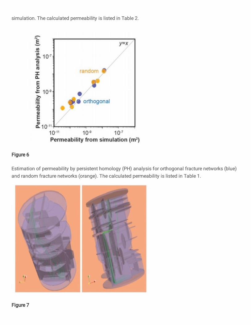
318 There is a limitation of Eq. (7). Eq. (7) is based on a parallel plate model, so the flow 319

is assumed to be straight. If there is tortuosity in a flow channel, the flow length will be longer, 320

and the estimated permeability may be larger than the true value. Figure 7 shows streamlines 321

in model O8 colored as green. We can see that the streamlines are winding and flowing. Keep 322

in mind the fact that tortuosity was not taken into account in Eq. (7). 323

324 Figure 7 | Streamlines (green lines) in fracture network simulated in OpenFOAM. 325

326 We also applied persistent homology analysis to other cases. Mehmani and Mamdi 327

(2015)39 conducted high-fidelity direct numerical simulation of the two-dimensional 328

micromodel to develop their pore network models. We used their 2D image data as shown in 329

Figure 8a and their results from direct numerical simulation. Comparison with persistent 330

homology analysis is plotted with red dots for regular pore structures and with purple dots for 331

12

Berea sandstone in Figure 8c. These results suggest that the proposed analysis can be used for 332

two-dimensional flow. 333

Andrew et al. (2014)40 used X-ray microtomography to obtain four types of 3D rock 334

image data, and they conducted flow experiment to measure the permeability. The X-ray 335

microtomography images of the rocks are shown in Figure 8b. Comparison with the 336

experimental results is plotted as green dots in Figure 8c. Permeability estimated by persistent 337

homology is larger than the experimental results. As mentioned before, Eq. (7) does not 338

consider the effect of tortuosity. Muljadi et al. (2016)41 calculated the tortuosity from the same 339

Bentheimer sandstone and the Estaillades carbonate images as 1.52 and 1.91, respectively. If 340

we take the tortuosity into account, the estimates of the permeability will be close to the 341

experimental values. The calculation of tortuosity in Muljadi et al. (2016)41 used the flow 342

velocity42,43. In contrast, the goal of this study is to estimate flow properties without flow 343

simulation, so that we need to obtain tortuosity in a different way based on image analysis. 344

Correlation between tortuosity and persistent homology parameters would be explored in 345

future studies. 346

347

348 Figure 8 | Estimation of permeability by persistent homology (PH) analysis. a 2D 349

images from Mehmani and Hamdi (2015)39, b 3D rock images from Andrew et al. 350

(2014)40, and c comparison with direct simulation and experiment. The values are 351

listed in Table 3. 352

353

354

355

356

357

358

359

360

361

362

363

364

365

13

Table 3 | Information of 2D pore39 and 3D rock images40 and their 366

permeability. 367

Model Image size

(pixels)

Domain size

(mm)

Simulation

result

PH

estimation

2D pore Square

3000 x

1500

20 mm

× 10 mm × 200 μm

3.13 × 10-10 1.54 × 10-9

GL-D1 1.92 × 10-10 2.74 × 10-10

GL-D2 1.70 × 10-10 4.96 × 10-10

GL-D3 1.47 × 10-10 7.98 × 10-10

GL-D4 1.44 × 10-10 9.71 × 10-10

GS-D1 9.77 × 10-10 5.19 × 10-9

GS-D2 9.75 × 10-10 3.34 × 10-9

GS-D3 9.60 × 10-10 2.43 × 10-9

GS-D4 9.18 × 10-10 2.67 × 10-9

P-D1 3.25 × 10-10 1.75 × 10-9

P-D4 4.01 × 10-10 1.53 × 10-9

Berea 2900 x

2320

1.774 mm ×1.418 mm

× 24.54 μm

1.45 × 10-12 5.06 × 10-12

Model Image size

(voxels)

Resolution (um/px)

Experimental result

PH estimation

3D rock Doddington

300 x 300 x 300

2.6929 1.04 × 10-12 3.37 × 10-11

Bentheimer 3.0035 1.88 × 10-12 9.02 × 10-11

Ketton 3.00006 2.81 × 10-12 6.86 × 10-11

Estaillades 3.31136 1.49 × 10-13 2.90 × 10-11

368

Discussions 369

Persistent homology analysis could estimate opening aperture distributions of flow 370

channels and estimated permeability with the same order of magnitude as the permeability 371

derived from the simulation. Using this method, flow characteristics can be estimated from the 372

image data without the need for fluid flow simulation. This could make the analysis of fracture 373

networks quicker. In this study, the longest direct flow simulation took 72 hours to generate a 374

sufficiently high-resolution computational mesh then solve the Navier-Stokes equations, using 375

320 processors with a maximum of 282 GB of memory in a supercomputational system. In 376

contrast, persistent homology was able to calculate the model in less than 10 minutes with 16 377

GB of memory using a desktop workstation AMD Ryzen 9 5950X. 378

Several approaches44–46 based on discrete fracture network represent fractures as 379

ellipses or rectangles in networks based on Eq. (2). Focusing on the fractures themselves is 380

suitable for fractured rock bodies, but it may be difficult to optimize the model because of the 381

increase in number of parameters when the fractures are finer or when the body is regarded as 382

a porous medium. In this study, we focus on the flow channels by persistent homology instead 383

of individual fractures. Therefore, we can apply the method regardless of porous or fractured 384

rocks. 385

Recently, some studies have been published to investigate the relationship between 386

porous structures and flow by persistent homology29,30,47,48. Most of them were machine 387

learning approaches that put a large number of parameters into a black box. In contrast, since 388

our approach focuses on flow-channel structures, permeability can be calculated by the simple 389

and easy principle. We used the synthetic fracture networks as well as natural rocks. Although 390

the estimation errors were relatively large for 3D rocks, it was shown that a simple model such 391

as Eq. (7) can provide reasonably close estimates. 392

Ushizima et al. (2012)26 estimates permeability of porous rocks by using Reeb graphs 393

to represent the pore networks. They use persistent homology to distinguish between 394

significant and noisy pore spaces, and to supplement the Reeb graphs. In fact, the Reeb graph 395

14

and persistent homology were used independently and separately. We think that using Reeb 396

graphs is a good direction to go to the next step. 397

We have succeeded in modeling physical phenomena from image data based on the 398

topological data analysis. The method could be applied also to a wide range of porous media 399

including artificial devices. It is expected to be applicable not only to estimate flow properties, 400

but also to characterize different transport phenomena, such as mass transfer, electrical and 401

magnetic flows. 402

403

Method 404

Persistent homology analysis 405

STL files of synthetic fracture networks were generated by using OpenSCAD, and the 406

STL files were converted to the cross-sectional images in 36 mm × 36 mm × 50 mm with a 407

voxel resolution of 0.1 mm in Autodesk Netfabb. To eliminate some unexpected noises, all the 408

images were blurred in XnConvert. The png files of the image data were analyzed in 409

HomCloud63. When there were small differences between birth and death of PH1, the hole 410

structure may appear during the image analysis. Thus, we neglected the result with di - bi < 2 411

were eliminated. 412

413

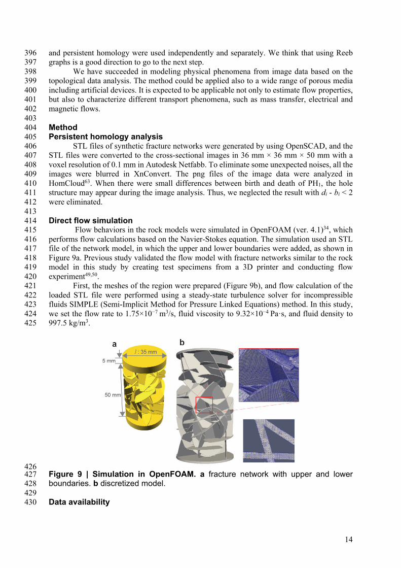
Direct flow simulation 414 Flow behaviors in the rock models were simulated in OpenFOAM (ver. 4.1)34, which 415

performs flow calculations based on the Navier-Stokes equation. The simulation used an STL 416

file of the network model, in which the upper and lower boundaries were added, as shown in 417

Figure 9a. Previous study validated the flow model with fracture networks similar to the rock 418

model in this study by creating test specimens from a 3D printer and conducting flow 419

experiment49,50. 420

First, the meshes of the region were prepared (Figure 9b), and flow calculation of the 421

loaded STL file were performed using a steady-state turbulence solver for incompressible 422

fluids SIMPLE (Semi-Implicit Method for Pressure Linked Equations) method. In this study, 423

we set the flow rate to 1.75×10−7 m3/s, fluid viscosity to 9.32×10−4 Pa·s, and fluid density to 424

997.5 kg/m3. 425

426 Figure 9 | Simulation in OpenFOAM. a fracture network with upper and lower 427

boundaries. b discretized model. 428

429

Data availability 430

15

The data that support the findings of this study are available in 431

https://figshare.com/s/cebf663b253d145bf8ac (doi: 10.6084/m9.figshare.14110262, active 432

when the item is published), https://figshare.com/s/de6df5d1cf76926c7f25 (doi: 433

10.6084/m9.figshare.14110208), https://figshare.com/s/96f9d83791dc03e28ce0 (doi: 434

10.6084/m9.figshare.14113439). 435

436

Reference 437

1. Renard, P. & de Marsily, G. Calculating equivalent permeability: a review. Adv. 438

Water Resour. 20, 253–278 (1997). 439

2. Costa, A. Permeability-porosity relationship: A reexamination of the Kozeny-440

Carman equation based on a fractal pore-space geometry assumption. 441

Geophys. Res. Lett. 33, 1–5 (2006). 442

3. Carman, P. C. Fluid flow through granular beds. Trans. Chem. Eng. 15, S32–443

S48 (1937). 444

4. Zimmerman, R. W. & Bodvarsson, G. S. Effective transmissivity of two-445

dimensional fracture networks. Int. J. Rock Mech. Min. Sci. Geomech. Abstr. 446

33, 433–438 (1996). 447

5. Snow, D. Anisotropic Permeability o[ Fractured Media. Water Resour. Res. 5, 448

1273–1289 (1969). 449

6. Renshaw, C. E. On the relationship between mechanical and hydraulic 450

apertures in rough-walled fractures. J. Geophys. Res. 100, 629–636 (1995). 451

7. Witherspoon, P. A., Wang, J. S. Y., Iwai, K. & Gale, J. E. Validity of Cubic Law 452

for fluid flow in a deformable rock fracture. Water Resour. Res. 16, 1016–1024 453

(1980). 454

8. Zimmerman, R. & Yeo, I. Fluid Flow in Rock Fractures: From the Navier-455

Stokes Equations to the Cubic Law. Dyn. fluids Fract. rock 213–224 (2000). 456

doi:10.1029/GM122p0213 457

9. Hyman, J. D., Aldrich, G., Viswanathan, H., Makedonska, N. & Karra, S. 458

Fracture size and transmissivity correlations: Implications for transport 459

simulations in sparse three-dimensional discrete fracture networks following a 460

truncated power law distribution of fracture size. Water Resour. Res. 5, 2–2 461

(1969). 462

10. Valentini, L., Perugini, D. & Poli, G. The “small-world” topology of rock fracture 463

networks. Phys. A Stat. Mech. its Appl. 377, 323–328 (2007). 464

11. Andresen, C. A., Hansen, A., Le Goc, R., Davy, P. & Hope, S. M. Topology of 465

fracture networks. Front. Phys. 1, 1–5 (2013). 466

12. Mecke, K. & Arns, C. H. Fluids in porous media: A morphometric approach. J. 467

Phys. Condens. Matter 17, (2005). 468

13. Lehmann, P. et al. Impact of geometrical properties on permeability and fluid 469

phase distribution in porous media. Adv. Water Resour. 31, 1188–1204 (2008). 470

14. Scholz, C. et al. Permeability of porous materials determined from the Euler 471

characteristic. Phys. Rev. Lett. 109, 1–5 (2012). 472

15. Liu, Z., Herring, A., Arns, C., Berg, S. & Armstrong, R. T. Pore-Scale 473

Characterization of Two-Phase Flow Using Integral Geometry. Transp. Porous 474

Media 118, 99–117 (2017). 475

16. Armstrong, R. T. et al. Porous Media Characterization Using Minkowski 476

Functionals: Theories, Applications and Future Directions. Transp. Porous 477

Media 130, 305–335 (2019). 478

17. Edelsbrunner, H. & Harer, J. Persistent homology—a survey. Contemp. Math. 479

257–282 (2008). doi:10.1090/conm/453/08802 480

16

18. Zomorodian, A. & Carlsson, G. Computing persistent homology. Proc. Annu. 481

Symp. Comput. Geom. 274, 347–356 (2004). 482

19. Edelsbrunner, H. & Morozov, D. Persistent Homology : Theory and Practice. in 483

Conference: European Congress of Mathematics (2012). 484

20. Weinberger, S. What is Persistent Homology? Am. Math. Soc. 58, 36–39 485

(2010). 486

21. Chazal, F. & Michel, B. An introduction to topological data analysis: 487

Fundamental and practical aspects for data scientists. arXiv 1–38 (2017). 488

22. Otter, N., Porter, M. A., Tillmann, U., Grindrod, P. & Harrington, H. A. A 489

roadmap for the computation of persistent homology. EPJ Data Sci. 6, (2017). 490

23. Kimura, M., Obayashi, I., Takeichi, Y., Murao, R. & Hiraoka, Y. Non-empirical 491

identification of trigger sites in heterogeneous processes using persistent 492

homology. Sci. Rep. 8, 1–9 (2018). 493

24. Hiraoka, Y. et al. Hierarchical structures of amorphous solids characterized by 494

persistent homology. Proc. Natl. Acad. Sci. U. S. A. 113, 7035–7040 (2016). 495

25. Ichinomiya, T., Obayashi, I. & Hiraoka, Y. Persistent homology analysis of 496

craze formation. Phys. Rev. E 95, 1–6 (2017). 497

26. Ushizima, D. et al. Augmented topological descriptors of pore networks for 498

material science. IEEE Trans. Vis. Comput. Graph. 18, 2041–2050 (2012). 499

27. Robins, V., Saadatfar, M., Delgado-Friedrichs, O. & Sheppard, A. P. 500

Percolating length scales from topological persistence analysis of micro-CT 501

images of porous materials. Water Resour. Res. 52, 315–329 (2016). 502

28. Tsuji, T., Jiang, F., Suzuki, A. & Shirai, T. Mathematical Modeling of Rock Pore 503

Geometry and Mineralization: Applications of Persistent Homology and 504

Random Walk. 95–109 (2018). doi:10.1007/978-981-10-7811-8_11 505

29. Jiang, F., Tsuji, T. & Shirai, T. Pore Geometry Characterization by Persistent 506

Homology Theory. Water Resour. Res. 54, 4150–4163 (2018). 507

30. Herring, A. L., Robins, V. & Sheppard, A. P. Topological Persistence for 508

Relating Microstructure and Capillary Fluid Trapping in Sandstones. Water 509

Resour. Res. 55, 555–573 (2019). 510

31. Suzuki, A. et al. Inferring fracture forming processes by characterizing fracture 511

network patterns with persistent homology. Comput. Geosci. 143, 104550 512

(2020). 513

32. Obayashi, I. & Hiraoka, Y. Persistence diagrams with linear machine learning 514

models. arXiv 1, 421–449 (2017). 515

33. Choudhury, a. N. M. I., Wang, B., Rosen, P. & Pascucci, V. Topological 516

analysis and visualization of cyclical behavior in memory reference traces. 517

2012 IEEE Pacific Vis. Symp. 9–16 (2012). 518

doi:10.1109/PacificVis.2012.6183557 519

34. Choudhury, A. N. M. I., Wang, B., Rosen, P. & Pascucci, V. Topological 520

analysis and visualization of cyclical behavior in memory reference traces. 521

IEEE Pacific Vis. Symp. 2012, PacificVis 2012 - Proc. 9–16 (2012). 522

doi:10.1109/PacificVis.2012.6183557 523

35. Martys, N. & Garboczi, E. J. Length scales relating the quid permeability and 524

electrical conductivity in random two-dimensional model porous media. Phys. 525

Rev. B 46, 6080–6090 (1992). 526

36. Schwartz, L. M., Martys, N., Bentz, D. P., Garboczi, E. J. & Torquato, S. 527

Cross-property relations and permeability estimation in model porous media. 528

Phys. Rev. E 48, 4584–4591 (1993). 529

37. Nishiyama, N. & Yokoyama, T. Permeability of porous media: Role of the 530

17

critical pore size. J. Geophys. Res. Solid Earth 122, 6955–6971 (2017). 531

38. Watanabe, K. & Takahashi, H. Fractal geometry characterization of 532

geothermal reservoir fracture networks. Journal of Geophysical Research 100, 533

521–528 (1995). 534

39. Mehmani, Y. & Tchelepi, H. A. Minimum requirements for predictive pore-535

network modeling of solute transport in micromodels. Adv. Water Resour. 108, 536

83–98 (2017). 537

40. Andrew, M., Bijeljic, B. & Blunt, M. J. Pore-scale imaging of trapped 538

supercritical carbon dioxide in sandstones and carbonates. Int. J. Greenh. Gas 539

Control 22, 1–14 (2014). 540

41. Muljadi, B. P., Blunt, M. J., Raeini, A. Q. & Bijeljic, B. The impact of porous 541

media heterogeneity on non-Darcy flow behaviour from pore-scale simulation. 542

Adv. Water Resour. 95, 329–340 (2016). 543

42. Duda, A., Koza, Z. & Matyka, M. Hydraulic tortuosity in arbitrary porous media 544

flow. Phys. Rev. E - Stat. Nonlinear, Soft Matter Phys. 84, 1–8 (2011). 545

43. Koponen, I. Analytic approach to the problem of convergence of truncated 546

Levy flights towards the Gaussian stochastic process. Phys. Rev. E 52, 1197–547

1199 (1995). 548

44. Jing, Y., Armstrong, R. T. & Mostaghimi, P. Image-based fracture pipe network 549

modelling for prediction of coal permeability. Fuel 270, 117447 (2020). 550

45. Srinivasan, S., Karra, S., Hyman, J., Viswanathan, H. & Srinivasan, G. Model 551

reduction for fractured porous media: a machine learning approach for 552

identifying main flow pathways. Comput. Geosci. 23, 617–629 (2019). 553

46. Srinivasan, G. et al. Quantifying Topological Uncertainty in Fractured Systems 554

using Graph Theory and Machine Learning. Sci. Rep. 8, 1–11 (2018). 555

47. Robinson, J. et al. Imaging pathways in fractured rock using three-dimensional 556

electrical resistivity tomography. Groundwater 54, 186–201 (2016). 557

48. Thakur, M. M., Kim, F., Penumadu, D. & Herring, A. Pore Space and Fluid 558

Phase Characterization in Round and Angular Partially Saturated Sands Using 559

Radiation-Based Tomography and Persistent Homology. Transp. Porous 560

Media (2021). doi:10.1007/s11242-021-01554-w 561

49. Suzuki, A., Watanabe, N., Li, K. & Horne, R. N. Fracture network created by 3-562

D printer and its validation using CT images. Water Resour. Res. (2017). 563

doi:10.1002/2017WR021032 564

50. Suzuki, A., Minto, J. M., Watanabe, N., Li, K. & Horne, R. N. Contributions of 565

3D Printed Fracture Networks to Development of Flow and Transport Models. 566

Transp. Porous Media 129, 485–500 (2019). 567

568

Acknowledgements 569 Anna Suzuki was supported by JSPS KAKENHI Grant Numbers JP20H02676 and 570

JP17H04976 (Japan); JST ACT-X Grant Number JPMJAX190H (Japan). Ippei Obayashi was 571

supported by JSPS KAKENHI Grant Number JP 16K17638, JP 19H00834, JP 20H05884; 572

JST PRESTO Grant Number JPMJPR1923; JST CREST Mathematics Grant number 573

15656429 (Japan); and the Structural Materials for Innovation, Strategic Innovation 574

Promotion Program D72 (Japan), which are gratefully acknowledged. The authors would like 575

to thank Department of Earth Science and Engineering, Imperial College London for sharing 576

the micro-CT data of the rocks. These micro-CT data can be downloaded through their web 577

page: http://www.imperial.ac.uk/earth-sci- ence/research/research-groups/perm/ 578

research/pore-scale-modelling/micro- ct-images-and-networks/. 579

580

18

Author contributions 581 A.S. initiated the key concepts, designed, conducted persistent homology analysis, and 582

supervised the research. M.M. performed numerical simulation and conducted persistent 583

homology analysis. J.M. assisted flow simulation. I.O. and Y.H. assisted persistent homology 584

analysis. T.T and T.I conducted project administration. A.S. wrote the original draft. J.M., 585

I.O., Y.H., T.T and T.I reviewed and edited the manuscript. 586

587

Conflicts of Interest 588

The authors declare no conflict of interest. 589

Figures

Figure 1

Persistent homology analysis for fracture networks by HomCloud32 . a 3D view and b cross-sectionalimage of fracture network with a �ow channel (light blue arrow) and an isolated pore (mentioned asgreen). c Schematic of �ltration process. Image at t = -1 is the original image. White grids express voidspaces. Blue grids are the grids that were removed during the thinning process. Red grids are the gridsthat were added during the thickening process.

Figure 2

Detecting �ow channels using inverted images a ring-shaped, internal void-structure that is not connectedto the outside, and b its inverted image. c ring shaped, internal void-structure with two channels that isconnected to the outside and forms a �ow channel. d its inverted image. The left column shows 3D viewof images. The center column describes processes of �ltration. The right column lists Betti numbers β1.

Figure 3

Fractured models. a outside and b inside of model. c Orthogonal distribution and d random distribution offracture networks.

Figure 4

Estimation of fracture apertures by persistent homology (PH) analysis. a orthogonal fracture networksand b random fracture networks.

Figure 5

Validation with simple models. a one or two fracture penetrating the model. The top and bottom are theinlet and the outlet. b Comparison of permeability between persistent homology (PH) analysis and direct

simulation. The calculated permeability is listed in Table 2.

Figure 6

Estimation of permeability by persistent homology (PH) analysis for orthogonal fracture networks (blue)and random fracture networks (orange). The calculated permeability is listed in Table 1.

Figure 7

Streamlines (green lines) in fracture network simulated in OpenFOAM

Figure 8

Estimation of permeability by persistent homology (PH) analysis. a 2D images from Mehmani and Hamdi(2015)39, b 3D rock images from Andrew et al. (2014)40 , and c comparison with direct simulation andexperiment. The values are listed in Table 3.

Figure 9

Simulation in OpenFOAM. a fracture network with upper and lower boundaries. b discretized model.