flow distribution and heat transfer coefficients
TRANSCRIPT

FLOW DISTRIBUTION AND HEAT TRANSFER COEFFICIENTS INSIDE GAS HOLES
DISCHARGING
A Thesis
Submitted to the Graduate Faculty of the
Louisiana State University and
Agricultural and Mechanical College
in partial fulfillment of the
requirements for the degree of
Master of Science in Mechanical Engineering
in
The Department of Mechanical Engineering
by
Amirhossein Eshtiaghi
B.S., University of Tehran, 2005
December 2012

ii
Acknowledgements
I would like to thank my advisor, Dr. Sumanta Acharya for his support and advice since
January 2009. I would also like to thank Dr. Dimitris Nikitopoulos and Dr. Ingmar Schoegl for
being part of my advisory committee.
Moreover, I would like to thank my gorgeous wife Forough and cute son Arnick for their
support and patience during these years. Also, special thank to my father, Hassan, who showed
me the right path of life and supported me in this way and my mother, Fereshteh, who always
concerns about me.
Because the work presented in this Thesis is part of a project conducted by a team of
graduate students, I would also like to acknowledge Krishnendu Saha and Derrick Goss who
have been my lab partners during these years and Srinibas Karmakar, Baine Bereaux, Shengrong
Zhu, Del Segura and James Post, for their technical advises. I would also like to thank my
parents for their support in this adventure.
iii
Table of Contents
Acknowledgements ......................................................................................................................... ii
List of Figures ................................................................................................................................. v
Abstract .......................................................................................................................................... ix
Chapter 1: Introduction ................................................................................................................... 1
Chapter 2 Literature Review ........................................................................................................... 7
2.1 Flow inside short cooling holes ........................................................................................ 7
2.2 Cooling holes inlet modification .................................................................................... 10
2.3 Active control of jet mixing ........................................................................................... 12
Chapter 3:Experimental Methods and Apparatus ......................................................................... 18
3.1 Test section design ......................................................................................................... 18
3.1.1 Baffled test model ................................................................................................... 22
3.1.2 Excited flow test section ......................................................................................... 23
3.2 Wind tunnel .................................................................................................................... 24
3.3 Heat transfer coefficient calculation by wall temperature ............................................. 26
3.4 Temperature measurement inside gas holes ................................................................... 28
3.4.1 Infra red camera thermography ............................................................................... 28
3.4.2 Liquid crystal thermography ................................................................................... 30
3.5 Flow field parameters measurement .............................................................................. 31
3.5.1 Pressure measurement along plenum ...................................................................... 31
3.5.2 Velocity measurement inside gas holes by Pitot static tube ................................... 32
3.5.3 Velocity measurement outside gas holes by Pitot static tube ................................. 33
3.5.4 Near wall velocity measurement ............................................................................. 33
3.5.5 Velocity measurement by Hotwire ......................................................................... 35
3.5.6 Particle Image Velocimetry .................................................................................... 36
3.5.7 High speed flow visualization ................................................................................. 38
3.6 Error analysis of experimental methods ......................................................................... 41
3.6.1 Different heat transfer measurement methods ........................................................ 41
3.6.2 Uncertainty analysis ................................................................................................ 42
Chapter 4: Numerical Simulation ............................................................................................... 455
4.1 Reynolds-averaged Navier-Stokes equations (RANS) .................................................. 45
4.1.1 Flow simulation inside one gas hole ....................................................................... 45
4.1.2 Flow simulation inside the complete test model ..................................................... 49
Chapter 5: Results and Discussion ................................................................................................ 51
5.1 Pressure test .................................................................................................................... 51
5.2 Velocity measurements outside a gas hole ..................................................................... 52
5.3 In hole velocity fields ..................................................................................................... 53

iv
5.4 Heat transfer ................................................................................................................... 59
5.5 Hole configurations ........................................................................................................ 71
5.6 Geometry modification .................................................................................................. 73
5.6.1 Baffles placed downstream holes 1 and 2 ............................................................... 74
5.6.2 Baffles placed upstream all holes ........................................................................... 78
5.6.3 Velocity prediction.................................................................................................. 79
5.6.4 Variable baffles height ............................................................................................ 80
5.7 Active controlling of jet mixing ..................................................................................... 93
5.7.1 The jet natural frequency measurement .................................................................. 93
5.7.2 Jet excitation at different frequencies ..................................................................... 96
Chapter 6: Conclusion................................................................................................................. 108
Works Cited ................................................................................................................................ 110
Vita.. ................................................................................................................................ ………115
v
List of Figures
Figure 1. Typical gas turbine engine ............................................................................................................. 3
Figure 2. Gas turbine blade with cooling holes and squealer rim ................................................................. 4
Figure 3. Schematic of fuel-air premixing device ......................................................................................... 5
Figure 4. Schematic of real fuel premixer geometry (left) and experimental scaled model (right) ............ 18
Figure 5. Test section components .............................................................................................................. 19
Figure 6. Different gas holes arrangements along the plenum channel ...................................................... 22
Figure 7. Straight baffle shape and location inside the plenum .................................................................. 23
Figure 8. Test section geometry for active jet controlling experiment ....................................................... 24
Figure 9. Schematic view of wind tunnel and test model ........................................................................... 25
Figure 10. Air temperature variation during experiments inside gas holes ................................................ 28
Figure 11. Infrared camera location above the wind tunnel looking into gas holes.................................... 29
Figure 12. Zinc-Selenide window located in plexiglas holder .................................................................... 30
Figure 13. Temperature reading between IR-camera and thermocouple .................................................... 31
Figure 14. Schematic of pressure tap holes locations ................................................................................. 32
Figure 15. Pitot tube probe location for in hole velocity measurements ..................................................... 33
Figure 16. Pitot tube measurement locations outside gas holes .................................................................. 34
Figure 17. Five holes Pitot tube probe ........................................................................................................ 35
Figure 18. Optical configuration of laser head, optical elbow and PIV cameras ........................................ 38
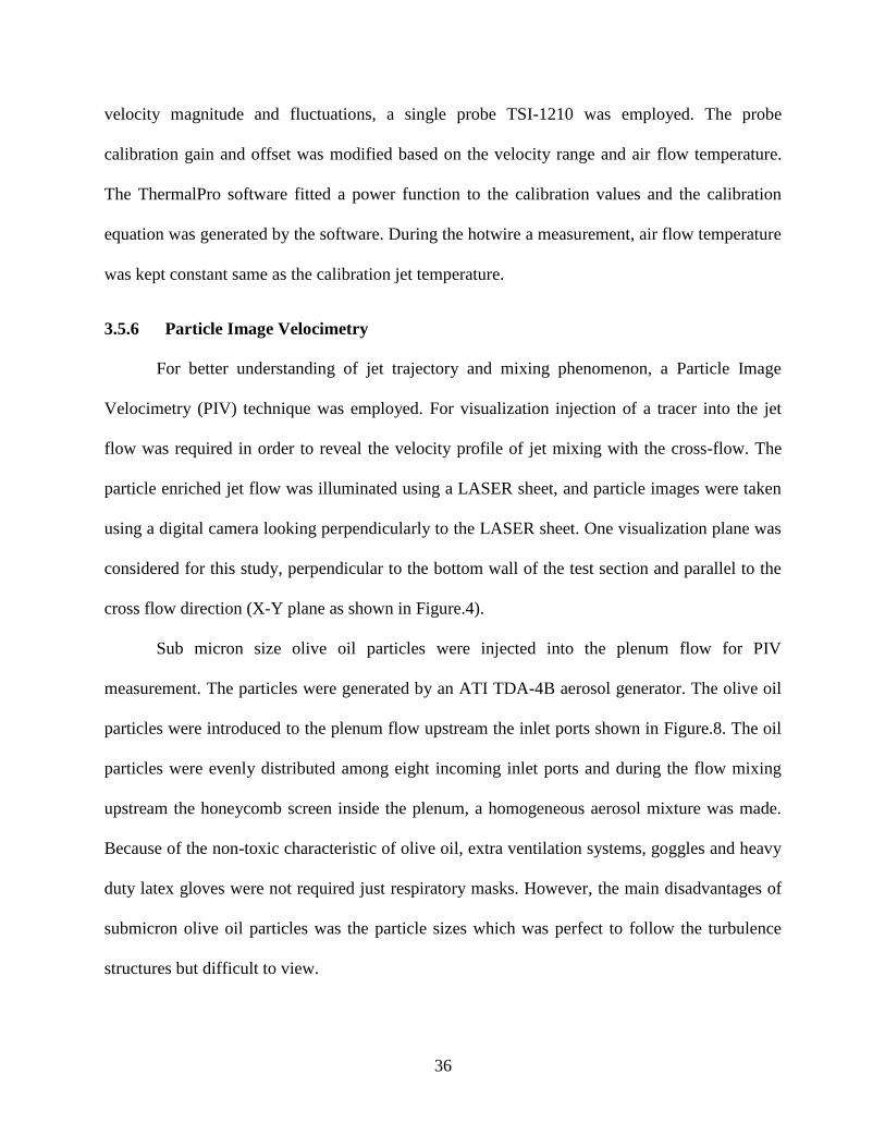
Figure 19 Vertical LASER sheet and Photron camera configuration ......................................................... 39
Figure 20 Intensity averaged image with various number of averaging samples ....................................... 40
Figure 21 Pixel intensity along red dotted line ........................................................................................... 41
Figure 22. Comparison of three methods on HTC calculation ................................................................... 42
Figure 23. Variation of measured HTC at two different locations inside gas hole 1 versus time ............... 44

vi
Figure 24. Schematic of one gas hole geometry with appropriate boundary conditions ............................ 46
Figure 25. Numerical grid inside one gas hole geometry a) whole geometry b) plenum wall and hole inlet
c) inside the hole d) test section surface and hole exit ................................................................................ 48
Figure 26. Variation of wall shear stress on the aft-side of the hole with grid size .................................... 49
Figure 27. Numerical simulation domain for complete test geometry ........................................................ 50
Figure 28 Experimental pressure inside the plenum at windward and leeward sides of holes ................... 52
Figure 29 Velocity profile inside the tunnel after hole 3 at specified distances ......................................... 53
Figure 30 Velocity distribution inside the holes 1 to 5 for the basic configuration at different and
BR=2.65 a) along line I, b) along line C ..................................................................................................... 54
Figure 31 Y-velocity contours and stream lines in holes 1 to 5 a) along line I b) along a line perpendicular
to line I ........................................................................................................................................................ 57
Figure 32 Predicted temperature profile and stream traces inside the holes a) along plane I and b) along
plane C. ....................................................................................................................................................... 58
Figure 33 Normalized Nusselt number in hole contour maps for basic configuration, BR=2.65 a)
Re=0.5x10⁵, b) Re=1.2x10
5, c) Re=1.7x10
5, d) Re=2.0x10
5 ...................................................................... 60
Figure 34 Circumferential variation of HTC at the inlet of gas holes 1 to 5 at Y/D=0.05 for basic
configuration (Re=1.7x10⁵ and BR=2.65) .................................................................................................. 61
Figure 35 predicted and experimental normalized Nusselt number at Y/D=0.05 for basic configuration
(Re=1.7x10⁵ and BR=2.65) ......................................................................................................................... 62
Figure 36 Variation of circumferentially averaged heat transfer coefficient along gas holes (Re=1.7x10⁵
and BR=2.65) .............................................................................................................................................. 63
Figure 37 Planar isotherms contour inside 5th hole for Re=1.7x10⁵ (left) and Re=0.5x10
5 (right) ........... 64
Figure 38 a) Normalized Nusselt number for basic case, Re=1.7x10⁵, BR=2.65. b) near wall velocity
contour map ................................................................................................................................................ 65
Figure 39 Comparison between experimental and predicted near wall velocity at Y/D=0.7. Re=1.7x10⁵
and BR=2.65 ............................................................................................................................................... 66
Figure 40 Variation of maximum normalized Nusselt number on the aft-side Vs Re (left) and ReL (right)
.................................................................................................................................................................... 67
Figure 41 Variation of averaged Nusselt number Vs Re (left) and ReL (right) (BR=2.65) ........................ 68

vii
Figure 42 Averaged Nusselt number inside hole 5 and a short hole with axisymmetrical entrance flow
versus ReL ................................................................................................................................................... 70
Figure 43 variation of averaged Nusselt number in holes 1 and 5 vs blowing ratio ................................... 70
Figure 44 Normalized Nusselt number contour maps inside each hole for configurations A to D ............ 72
Figure 45 Averaged normalized Nusselt number in holes for different configurations, (Re=1.7x10⁵,
BR=2.65) ..................................................................................................................................................... 73
Figure 46 Qualitative flow pattern inside the feed hole without baffles (left) and with baffles (right) ...... 75
Figure 47 Velocity comparison between first baffled and non-baffled cases ............................................. 76
Figure 48 Normalized heat transfer coefficient contour plots inside gas holes 1 to 5 for baffled (left) and
non-baffled (right) geometries .................................................................................................................... 77
Figure 49 Schematic of fluid flow inside the feed hole without baffles (left) and second baffles
arrangement (right) ..................................................................................................................................... 79
Figure 50 Velocity contour plots and stream traces inside all holes for a) non-baffled geometry, b) Second
baffled arrangement .................................................................................................................................... 81
Figure 51 Effect of baffle distance on flow structure inside one gas hole ((Re) ̅=1.7×10⁵, BR=2.65) ....... 83
Figure 52 Flow structure inside a gas hole for H/S ratio greater than one (Re=1.7×10⁵, BR=2.65) .......... 83
Figure 53 Normalized static pressure trend inside plenum (solid symbols), mass flow rate percentage of
each gas hole (hollow symbols) ((Re) ̅=1.7×10⁵, BR=2.65) ....................................................................... 86
Figure 54 Stream traces and normalized velocity (V/Vmax) contour maps inside gas holes 1 to 5 for a) non-
baffled (21) and b) modified baffled arrangements (Re=1.7×10⁵, BR=2.65) ............................................. 88
Figure 55 Predicted and measured normalized velocity values for best baffle arrangement and
experimental velocity values for non-baffled (21). (Re=1.7×10⁵, BR=2.65) ............................................. 89
Figure 56 Heat transfer coefficient contour plots inside gas holes for a) modified baffle arrangement b)
non-baffled geometry (21) (Re=1.7×10⁵,BR=2.65) .................................................................................... 90
Figure 57 Circumferential variation of axially averaged Nusselt number. non-baffled case (21)(solid line),
baffled case (dash line) (Re=1.7×10⁵,BR=2.65) ......................................................................................... 92
Figure 58 Axial variation of circumferentially averaged Nusselt number. non-baffled case (21)(solid line),
baffled case (dash line) (Re=1.7×10⁵,BR=2.65) ......................................................................................... 92
Figure 59 Variation of averaged Nusselt number inside gas holes 1 to 5 for non-baffled configuration
(21)and baffled arrangement. (Re=1.7×10⁵,BR=2.65)................................................................................ 93
viii
Figure 60 Velocity contour maps above the jet hole at different elevations, Re=1.0×10⁵, Br=2.65 .......... 95
Figure 61 Velocity magnitude power spectrum at three different elevations above the jet, Re=1.0×10⁵,
Br=2.65 ....................................................................................................................................................... 96
Figure 62 RMS velocity at L/D=1.0 above the jet hole for three different excitation frequency,
Re=1.0×10⁵, Br=2.65 .................................................................................................................................. 97
Figure 63 Mean jet velocity at different perturbation frequencies, Re=1.0×10⁵, Br=2.65 ......................... 98
Figure 64 High speed flow visualization at different perturbation freqs, (vertical plane L/D=1.0)
Re=1.0×10⁵, Br=2.65 ................................................................................................................................ 100
Figure 65 Vortex formation above the jet column for perturbation frequency of f0/4 .............................. 101
Figure 66 Vortex growth for perturbation frequency of f0/2 ..................................................................... 102
Figure 67 LASER sheet location for horizontal flow visualization .......................................................... 103
Figure 68 High speed flow visualization at different perturbation freqs, (horizontal plane) Re=1.0×10⁵,
Br=2.65 ..................................................................................................................................................... 104
Figure 69 Time variation of jet shape within one excitation cycle for f0/4 case, ..................................... 105
Figure 70 Intensity averaged images for different excitation frequencies ................................................ 106
Figure 71 Jet trajectory boundaries extracted from Figure 70 .................................................................. 106

ix
Abstract
Fluid flow and heat transfer coefficient associated with flow inside short holes (L/D=1)
discharging orthogonally into a crossflow was investigated experimentally and numerically for
𝑅𝑒 ranging from 0.5×10⁵ to 2×10
5, and blowing ratio ranging from 1.3 to 3.2. The basic
configuration studied consists of a feed tube with five orthogonally located gas holes. Four
different hole configurations were studied. The transient heat transfer study employs an IR-
camera to determine the local heat transfer coefficient inside each hole. Velocity measurements
and numerical flow simulation were used to better understand the measured heat transfer
distribution inside the hole. The Nusselt number distribution along the hole surface exhibits
significant circumferential non-uniformity associated with impingement and separation, with
localized high heat transfer regions caused by flow impingement. The heat transfer coefficient
was observed to be a strong function of the Reynolds number, but a weak function of the
blowing ratio.
Moreover, Fluid flow and heat transfer coefficient inside gas holes was improved by
changing the plenum geometry for 𝑅𝑒 =1.7×10⁵, and blowing ratio of 2.65. To improve the flow
structure understanding inside plenum and gas holes, numerical simulation using FLUENT code
was employed and verified by experimental measurements. Heat Transfer coefficient contour
maps inside gas holes was measured experimentally using IR-camera thermography to
investigate the effect of plenum geometry modifications on thermal stresses generated inside gas
holes. Results indicate that placing straight baffles at the upstream of cooling holes inlet inside
the plenum eliminates vortex generation in the gas holes for H/S=1. The recirculation bubble at
the back of each baffle guides air to flow smoothly into cooling holes. Also, by varying baffle
height, plenum mass flow rate can be distributed evenly among all gas holes.

1
1 Chapter 1: Introduction
Transferring fluid energy to usable mechanical forms has been one of the main concerns
of great scientists since the days of Archimedes. Babylonian emperor planned to use wind power
for irrigation in the 17th
century BC and the Greeks invented water driven wheel in the 3rd
century BC as first generation of turbo machines. Current supersonic jet engines are the most
advanced generation of ancient windmill idea. Turbomachinery is a certain class of machines
demonstrates the fluid energy conversion process very intuitively. Compressors, pumps, turbines
and fans exchange energy between fluid and a rotating shaft. The fluid interaction with blades
mounted on turbomachinery shaft transfers the energy from or into the fluid. In pumps and
compressors, mechanical energy is introduced to the fluid by raising the pressure through
velocity changes. On the other hand, turbines extract the fluid energy and convert it into the
rotational movement of the shaft.
The first significant development in turbomachinery is John Barber, an Englishman
patent in 1791. The operation principle of this machine required that air and fuel from a gas
producer be compressed in different cylinders and then going to a combustion chamber. The
combustion products were flew through a nozzle onto a turbine. However, on that days, it was
not possible for the device to create enough power to both compress the air and to have power
left over to provide useful work.
In 1873, Franz Stolze, a German designed a 10-stage axial flow compressor with 15-stage
axial flow turbine machine. Air from the compressor was directed into a “U” tube heat exchanger
and then to a single combustor. At the same time, George Brayton, an American, built a
successful gas turbine engine based on thermodynamic cycle composed of two reversible
2
constant pressure processes and two adiabatic processes. The Brayton cycle is the basis of
current gas turbines. In 1882, the Norwegian Adgidius Elling started the construction of a gas
turbine with possessed a six stage centrifugal compressor. This turbine produced 11 horsepower
in 1903. Then, by reheating the air by the turbine exhaust gases through a heat exchanger, Elling
built a gas turbine with 44 horsepower output. In 1905 Armengaud Brothers have developed the
first truly practical gas turbine. They utilized a 25 stages centrifugal compressor with a pressure
ratio of 3 to 1. The turbine blade and cascade was water cooled and combustion gases passed
through a 16.5 feet long pipe to reach the turbine bucket. Combustion gases temperature was
reduced to something below 850oF before entering the turbine section. The useful output of this
turbine was 82 horsepower and analytical efficiency of 3 percent.
In 1930’s the first practical gas turbine began to be placed into commercial purposes
developed by Brown Boveri and Company in Switzerland. During a shop testing of a compressor
and turbine set, it was necessary for Brown Boveri to provide a combustion chamber in order to
simulate the heat of carbon burning process in oil refineries. With this setup, Brown Boveri
realized that the compressor, combustor and turbine provided for a workable gas turbine could be
employed for power generation purposes. They installed the first power generator gas turbine in
Neuchatel in Switzerland in 1939 with 4 megawatts output and turbine inlet temperature of
approximately 1020oF.
Since the jet engine appearance during World War II all aspects of aviation industry has
been revolutionized. So, a jet engine improvement was necessary to keep airplane fly faster,
longer and carry more payload. Different companies started to build commercial gas turbines and
tried to compete on durability and cost of operation. Based on Baryton thermodynamic cycle,
3
theoretical efficiency of gas turbine is increased by increasing the combustion products
temperature.
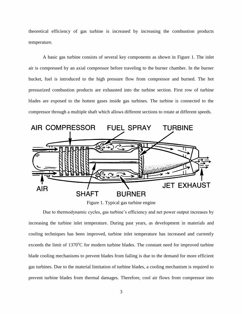
A basic gas turbine consists of several key components as shown in Figure 1. The inlet
air is compressed by an axial compressor before traveling to the burner chamber. In the burner
bucket, fuel is introduced to the high pressure flow from compressor and burned. The hot
pressurized combustion products are exhausted into the turbine section. First row of turbine
blades are exposed to the hottest gases inside gas turbines. The turbine is connected to the
compressor through a multiple shaft which allows different sections to rotate at different speeds.
Figure 1. Typical gas turbine engine
Due to thermodynamic cycles, gas turbine’s efficiency and net power output increases by
increasing the turbine inlet temperature. During past years, as development in materials and
cooling techniques has been improved, turbine inlet temperature has increased and currently
exceeds the limit of 1370oC for modern turbine blades. The constant need for improved turbine
blade cooling mechanisms to prevent blades from failing is due to the demand for more efficient
gas turbines. Due to the material limitation of turbine blades, a cooling mechanism is required to
prevent turbine blades from thermal damages. Therefore, cool air flows from compressor into
4
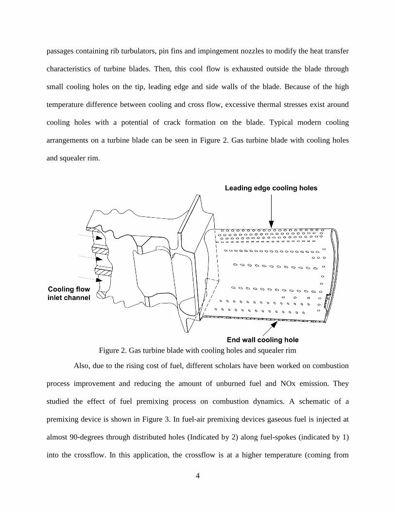
passages containing rib turbulators, pin fins and impingement nozzles to modify the heat transfer
characteristics of turbine blades. Then, this cool flow is exhausted outside the blade through
small cooling holes on the tip, leading edge and side walls of the blade. Because of the high
temperature difference between cooling and cross flow, excessive thermal stresses exist around
cooling holes with a potential of crack formation on the blade. Typical modern cooling
arrangements on a turbine blade can be seen in Figure 2. Gas turbine blade with cooling holes
and squealer rim.
Figure 2. Gas turbine blade with cooling holes and squealer rim
Also, due to the rising cost of fuel, different scholars have been worked on combustion
process improvement and reducing the amount of unburned fuel and NOx emission. They
studied the effect of fuel premixing process on combustion dynamics. A schematic of a
premixing device is shown in Figure 3. In fuel-air premixing devices gaseous fuel is injected at
almost 90-degrees through distributed holes (Indicated by 2) along fuel-spokes (indicated by 1)
into the crossflow. In this application, the crossflow is at a higher temperature (coming from
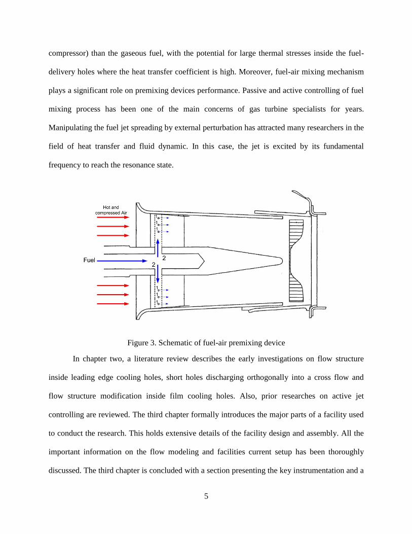
5
compressor) than the gaseous fuel, with the potential for large thermal stresses inside the fuel-
delivery holes where the heat transfer coefficient is high. Moreover, fuel-air mixing mechanism
plays a significant role on premixing devices performance. Passive and active controlling of fuel
mixing process has been one of the main concerns of gas turbine specialists for years.
Manipulating the fuel jet spreading by external perturbation has attracted many researchers in the
field of heat transfer and fluid dynamic. In this case, the jet is excited by its fundamental
frequency to reach the resonance state.
Figure 3. Schematic of fuel-air premixing device
In chapter two, a literature review describes the early investigations on flow structure
inside leading edge cooling holes, short holes discharging orthogonally into a cross flow and
flow structure modification inside film cooling holes. Also, prior researches on active jet
controlling are reviewed. The third chapter formally introduces the major parts of a facility used
to conduct the research. This holds extensive details of the facility design and assembly. All the
important information on the flow modeling and facilities current setup has been thoroughly
discussed. The third chapter is concluded with a section presenting the key instrumentation and a

6
detailed uncertainty analysis of all applicable parameters such as pressure, velocity and heat
transfer coefficient. Forth chapter talks about Numerical simulation parameters and strategies.
This chapter presents the equations required to simulate the flow structure inside cooling holes
along with turbulent modeling techniques and mesh grid structure. Pressure, velocity and heat
transfer data can be found in the fifth chapter. Contour plots show Numerical velocity profile and
experimental heat transfer coefficient inside cooling holes. Line plots have been chosen to
represent the agreement between numerically predicted values with experimentally measured
ones. Separate plots of averaged quantities summarize the thermal stresses behavior with flow
parameters of local Reynolds number and blowing ratio. Velocity profiles attained from particle
image velocimetry and high speed visualization images present the effect of flow excitation on
jet mixing. Explanation of these data sets specifies the author understands of these results and
their meaning. An outline of result and recommendations for future study covers the last chapter.
7
2 Chapter 2 Literature Review
2.1 Flow inside short cooling holes
Since the application of interest focuses primarily on the developing heat transfer in a
short hole with a complex entry, the relevant literature is rather limited with the majority of the
reported studies devoted to more conventional geometry and entry conditions (see Bejan (1)).
The heat transfer behavior in the developing region of a long circular pipe has been extensively
studied and entry-region correlations have been reported by Al-Arabi (2) and Ghajar (3). They
studied heat transfer in the developing region of a long circular pipe. Empirical correlations for
different Reynolds number and tube inlet shape were developed. Al-arabi studied a turbulent
flow and Ghajar studied laminar flow. In both cases, results show a high heat transfer coefficient
value at the tube inlet which decreases and flattens by moving down to the development region.
Sparrow & Cur (4), Han & Park (5) studied heat transfer coefficient inside a rectangular
duct with sudden-contraction. Results indicate that a recirculation bubble forms just at the
contraction region. Local heat transfer coefficient presents a sharp increasing trend to the point
where the recirculation bubble reattaches the channel wall. After this point, heat transfer
coefficient decreases gradually and then flattens at fully developed region.
Raisee and Hejazi (6) studied a developing turbulent flow through a straight rectangular
channel with sudden contraction numerically using SIMPLE algorithm with linear low Reynolds
number k-ε model. They reported formation of a recirculation bubble just downstream the
contraction point. This recirculation bubble triples the heat transfer coefficient where reattaches
the wall. Their predicted results follow experimentally measured values precisely at the
contraction region but not in the developing region. Nassab et al (7) performed a numerical
8
investigation about forced convection on an inclined forward step in a rectangular duct. Their
results indicate that inclination angle has a significant effect on heat transfer from the step. They
reported that heat transfer coefficient on the step increases by increasing the inclination angle
due to the change in recirculation bubble size.
Using naphthalene sublimation technique, Cho et al (8) investigated local heat transfer
inside a short circular hole with axisymmetrical inlet flow and Reynolds number ranging from
2×10³ to 3×10
4. Their results indicate existence of a reattachment region inside the hole and
strength of recirculation bubble was decreasing by increasing the Reynolds number to a certain
value and then remained constant. The heat transfer coefficient value at the reattachment point
was four times of heat transfer value of a fully developed pipe flow. Also in a similar study, Cho
and Goldstein (9) studied the effect of blowing ratio varying from 0.2 to 2.2 on heat transfer
inside short holes. Results indicate that for blowing ratio values smaller than 0.22, the
recirculation region inside the hole was shrunk by the cross flow. At higher blowing ratios larger
than mentioned value, recirculation region inside the gas hole was not affected by cross flow.
Also, they developed an empirical correlation for variation of average Nusselt number versus
Reynolds number.
In an experimental research about flow structure inside short channels, Cho et al (10)
looked into heat transfer and flow field inside a rectangular passage located orthogonally on a
plenum. The channel length was twice the hydraulic diameter and the flow structure showed a
recirculation structure at the inlet of the channel. Also, the heat transfer on the fore-side of the
channel exit was increasing by decreasing the blowing ratio because of the formation of a
secondary vortex.
9
To investigate the heat transfer coefficient distribution at the inlet of short holes
connected to a plenum, Goldstein et al (11) studied heat transfer inside a series of short holes
located orthogonally on a plenum wall experimentally. They used naphthalene sublimation
technique and results indicated that the velocity profile at the inlet of each hole can be a
combination of velocity profile inside a 90o bend and a sudden contraction. The mass transfer
coefficient inside short holes varied circumferentially due to separation zone. Also, the average
Sherwood number was greatest inside the hole closest to the plenum end.
Peterson and Plesniak (12) used particle image velocimetry to study velocity field in
detail in a film cooling hole discharging to a cross flow. Two different configurations of flow
supply plenum were investigated and compared. Their results indicate that plenum flow
configuration plays a significant role on short hole hydrodynamics. When the plenum flow was
in the same direction as cross flow, higher jet trajectory resulted at the hole exit comparing to a
situation that plenum flow is in the opposite direction of cross flow. The co-flow configuration
produces stronger counter rotating vortex pair than counter flow configuration.
In a detail numerical and experimental research, Ramamurthy et al (13) studied 3-
dimensional turbulent flow in a dividing T-junction. Results indicated that the flow inside the
main conduit is divided into two flows upstream the cross branch inlet. The entering flow into
the cross branch impinges aft-side of the tube inlet and a separation region forms on the fore-side
in front of the impingement region. The numerical predicted velocity field was verified by
experimentally measured pressure values. Wall pressure results inside the main conduit and on
the branch side illustrate a drastic drop upstream the branch due to the flow acceleration entering
into the branch.
10
Burd and Simon (14) and Hale et al (15), studied the effect of coolant flow supply
geometry on thermal effectiveness downstream the film cooling holes. Different coolant supply
geometries were experimented for different velocity ratios. Results document the effect of
plenum geometry on surface film cooling parameters. The flow patterns for different flow
configurations had been specified.
2.2 Cooling holes inlet modification
In gas turbine related literature, a vast variety of parameters have been investigated
experimentally and numerically. Ardey and Fottner (16), Chernobrovkin and Lakshminarayana
(17), Leylek and Zerkle (18), Papell (19) and Sinha et al (20) have studied film cooling
mechanism numerically and experimentally. However, they used an ideal plenum configuration
to provide air into the film cooling holes. In modern cooled turbine vane as shown in Figure 2,
film cooling holes at the leading edge of the vane are perpendicular to the supply plenum.
Therefore, cooling air turns sharply into gas holes and perfect plenum configuration is hardly
applicable as studied by Acharya et al (21).
Wilfert and Wolff (22)studied the effect of internal flow condition and plenum geometry
on film cooling effectiveness. They investigated the effect of conducting flow into the film
cooling holes by installing ribs inside the plenum on heat transfer downstream cooling holes.
Moreover, a vortex generator was designed and placed inside the plenum to introduce plenum air
smoothly into the cooling holes. Their results show 5 to 65 percent enhancement in film cooling
effectiveness comparing to a standard plenum configuration.
Vogel (23) studied the vortex generation and flow structure on a scaled airfoil at real flow
condition numerically. His investigation confirms the strong effect of inner contouring on film
cooling effectiveness. Thole et al (24) and Gritsch et al (25) used a narrow two-dimensional
11
coolant channel to investigate the effect of various parameters on film cooling performances.
Their results show a significant influence of varying cooling hole supply Mach number, hole
geometry, and inclination angle on the film cooling performance. Berhe and Patankar (26) found
that the influence of internal flow on film cooling effectiveness is strong while the plenum height
is twice the cooling holes diameter.
To improve the film cooling effectiveness by modifying the film cooling holes geometry,
Immarigeon and Hassan (27), studied a novel scheme in film cooling scheme numerically. They
combined in-hole impingement and flow turbulators to prevent jet lift off downstream the
cooling holes. They found that the film cooling jet remains attached to the wall at higher
blowing ratios, indicating an incredible performance for their proposed scheme. Their novel
scheme combined both advantages of impingement cooling and traditional film cooling to
provide a better blade protection. To improve the film cooling layer coverage on the blade
surface, Vogel (23), modified the cooling channel and film cooling holes design to generate
vortices and studied numerically. His research indicates that a vortex pair can be generated inside
the coolant channel which counter-rotates against the main kidney shaped vortex. This internally
generated vortex was moved from the jet centerline to the sides and provides coolant out of the
jet center. So a flat coolant film is generated downstream the cooling holes which improves the
film cooling effectiveness.
In an interesting experimental study, Lerch and Schiffer (28) investigated the effect of
flow condition inside the plenum on film cooling effectiveness employing ammonia-diazo
technique. A standard internal cross flow with a sharp edged inflow was compared with an
internal cyclone cooling airflow and film cooling effectiveness downstream cooling holes was
12
measured. Results indicate a significant change on film cooling effectiveness between standard
internal flow and swirled internal flow.
2.3 Active control of jet mixing
Aerodynamic characteristics of turbulent jets can be manipulated by periodical action on
the jet flow section. So, finding and quantifying the turbulent jet characteristics has received
much attention over the past decades. Very early studies on free shear flows were stochastic in
nature however the discovery of coherent structures in free shear layers has changed the direction
of researches in future. Brown and Roshko (29), studied the plane turbulent mixing between two
different gases flow. They found that for all ratios of densities in the two streams, large coherent
structures are dominated in the mixing layer. These structures move at nearly constant rate and
their size increases by merging with the neighboring structures. The density changes across the
mixing layer have small effects on the mixing layer spreading angle and when one stream is
supersonic, compressibility has the strongest effect.
Winant and Browand (30) and Ho and Huang (31), manipulated the large scale structures
drastically by introducing low amplitude forcing to the shear layer. The vortex roll-up process
were taken place in an organized fashion and structure merging could be delayed or promoted
depending on the ratio of forcing frequency to the shear layer natural frequency. For small
frequency ratios simultaneous interaction of more than two structures could be promoted. The
intense mixing occurs during pairing process as reported by Bernel and Roshko (32). Their
results indicate that at some distance downstream the dividing plate a secondary spanwise
instability appears leading to the development of stream wise vortices. The appearance of these
vortices promotes the mixing process due to the interaction of streamwise vortices with spanwise

13
structures. By increasing the downstream distance, the interaction increases the 3D structures in
the shear layer, leading to high-order instabilities.
In an axisymmetric jet flow layer leaving a round nozzle, the initial shear layer behavior
is similar to the planar shear layer. Downstream the jet, azimuthal modes in the shear layer
compete each other for growth. Also, the free shear layer grows toward the jet centerline and
merges on centerline which is the end of jet potential core. Plaschko (33), investigated the
growth of spiral modes in slowly diverging jets experimentally and numerically. His research
indicates that at high Strouhal number, instabilities grow very rapid and reach their maximum
amplification state at a short distance from the jet exit. In this case, axisymmetrical instabilities
grow faster than spiral instabilities. The linear stability study by Michalke (34), showed that
downstream the jet, where the velocity profile is bell shaped, only helical instabilities can be held
in the jet. Also the growth region of helical modes moves upstream by increasing the jet velocity.
Two structures interact with each other and merge if the downstream structure slows
down and upstream structure speeds up. Many researchers have studied the passage frequency of
large scale structures at the end of the jet potential core, named preferred jet frequency and
scaled it by jet nozzle diameter. Crow and Champagne (35), reported that an incompressible jet
can hold the orderly modes of axisymmetric jet. The preferred mode frequency can be calculated
from f=0.3Ue/D. The fundamental mode is able to attain the largest amplitude and its harmonics
are least effective. This mode is the most dispersive mode but it cannot have an extreme length.
So, they proposed an intermediate length of wavelength λ=2.38D. But, the preferred frequency
Strouhal number can vary in a wider range as reported by Zaman and Hussain (36) and Reynolds
and Bouchard (37), from 0.2 to 0.6.

14
Jet in cross flow can be controlled actively and passively. Researchers have modified the
jet nozzle edge to manipulate jet profile and velocity structure by tabs, chevrons and lobbed
nozzles. Passive jet control had attracted attentions primarily to mitigate the jet noise level. The
main mechanism in jet controlling is the stream wise vorticity generated by the geometrical
modification as reported by Zaman et al (38). They used small tabs in different shapes at the
nozzle exit to generate vortices. Each tab produces a dominant pair of counter rotating stream-
wise vortices which results in an inward indentation of the mixing layer into the jet center line.
Their results state that two delta tabs located in front of each other, completely bifurcate the jet.
Four delta tabs stretch the mixing layer into four fingers and enhances the mixing significantly.
But, six delta tabs distort the mixing layer to a three fingers configuration through an interaction
of the stream wise vortices. The tabs were found effective equally in both laminar and turbulent
jet flow. Depending on the tab orientation, a vortex pair can be produced rotating in the opposite
direction of the dominant pair. Investigations on passive enhancement of the jet spreading were
continued by Kumar et al (39) experimentally. They introduced square shape grooves both on
major and minor axis to study the jet flow development. Their results indicate that for Reynolds
number of 54000, introducing groves in major axis promotes the jet growth along major axis and
inhibit jet growth along minor axis.
In active controlling method, energy is added to the flow in a pulsative manner. The first
category of active controlling is low-frequency energy addition to the flow. The second category
involves using actuators with frequency capabilities in the range of flow instability frequencies.
Many researchers have contributed to the control of low-Reynolds number jets. The upper limit
of the Reynolds number based on jet diameter seems to be mostly around 50000. As the
Reynolds number increases, the instability frequency and flow momentum increases. But, the

15
number of researches on high Reynolds number jets is limited. Lepicovsky and Brown (40),
studied the effects of nozzle exit boundary layer on free jet excitation experimentally. They used
pressure sensors to measure the flow parameters at a Mach number of 0.8 and noise level of 147
dB. They found that the jet mixing depends strongly on boundary layer thickness and jets with a
thin laminar boundary layer are more sensitive to the preferred excitation frequency than jets
with thick boundary layer. Also, their results showed that the free jet mixing and development
can be controlled by both acoustic excitation and nozzle exit boundary layer.
In an experimental investigation on impingement heat transfer, Liu and Sullivan (41),
have studied the heat transfer in an excited circular jet impingement. The local heat transfer in
the wall-jet region was found very sensitive to the excitation frequency with small nozzle to plate
spacing. The local heat transfer coefficient manipulation was performed by forcing the jet near
the jet natural frequency and its sub-harmonics. They found that the phenomena of heat transfer
enhancement and reduction are related to the large scale vertical structures in the jet. When the
excitation frequency is close to the natural frequency, the initiated vortex pairing produces
turbulence which enhances the local heat transfer. When the forcing is near the subharmonic of
the natural frequency, stable vortex pairing is promoted. Pack and Seifert (42), studied the effects
of periodic excitation on turbulent jet. They used a short wide angle diffuser attached to the jet
exit and excitation was introduced between the jet exit and diffuser inlet. Their results indicated
that the jet deflection angle was very sensitive to the relative direction between the excitation and
the jet flow. However, diffuser angle was not affected by the excitation frequency.
In a qualitative investigation performed by Meyers et al (43), the vortex formation and
merging process was studied in the near field of a forced jet experimentally. The acoustic
perturbation was used to obtain a repeatable vortex pairing. The results indicated that the pairing
16
process was composed of several phases. First phase is vortex roll up which is laminar with
molecular diffusion. The next step was when the trailing vortex approaches and interferes with
the co-flow fluid entrainment. The gross deformation and stretching of the trailing vortex made
coalescence phase. The last step is re-entrainment of pure fluid after the pairing event.
In an experimental study, M’Closkey et al (44), investigated the dynamics of temporally
forced jet, injected orthogonally into a crossflow. A linear model for the forced jet actuation was
used to develop a dynamic compensator for the actuator. The application of the compensator
allowed significantly improved waveform at the jet exit. The optimum jet penetration was
observed to occur for square wave excitation at sub-harmonics of the vortex shedding frequency.
In all optimal cases, the wave duty cycles should be around 2.7-3.0 ms.
Hwang and Cho (45), conducted an experimental study to investigate the effect of
acoustic excitation on an impinging jet. They studied the effect of both main jet excitation and
shear layer excitation on local heat transfer. Their results showed that at excitation frequency of
St=1.2, the vortex pairing was promoted while low heat transfer rates were obtained at large
nozzle to plate distances. But, for the main jet excitation of St=2.4, heat transfer rates were high
at the large gap distance due to the extended potential core. In a similar study O’Donovan and
Murray (46), investigated the effect of high frequency excitation of impinging jets on surface
heat transfer. They reported that the vortex roll up has an influence on surface heat transfer for at
low nozzle to impingement surface spacing. Their results indicated that by increasing the
excitation frequency toward the naturally occurring frequency, the secondary peak magnitude in
Nusselt number was increased. Therefore, they anticipated that by increasing the excitation
frequency above the jet preferred mode, heat transfer magnitude could be enhanced.

17
In a recent numerical study, Muldoon and Acharya (47), simulated a jet with a passive
scalar injecting orthogonally into a crossflow at blowing ratio of 6 and Reynolds number of
5000. The jet flow was forced by sinusoidal function at different non-dimensional frequencies of
0.2, 0.4 and 0.6. The unforced jet preferred frequency was determined to be around 0.35 but with
forcing, the dominant frequency near the jet field was the forcing frequency. However, further
downstream the jet due to vortex interactions, subharmonic modes grow and at forcing frequency
of 0.2, the jet bifurcates in vertical plane. At the forcing frequency of 0.4, the jet trifurcates into
three jet streams in the vertical plane and at forcing frequency of 0.6 the jet bifurcates in the
horizontal plane. They reported that, U-loop structures at the wake region were seen for all
frequencies except for 0.6 where they are completely suppressed. The U-loop structure was
symmetrical for the unforced and 0.2 forcing modes.
Roux et al (48), investigated the effect of jet excitation on impingement heat transfer.
They used two different configurations of nozzles at three different nozzle to plate distances and
jet Reynolds number of 28,000. The jet excitation Strouhal number was changing from 0.26 to
0.79 using a high power loudspeaker. Their results indicated that the acoustic forcing modified
flow structure and created annular vortex rings in the jet shear layer. The merging phenomenon
happens for high Strouhal number forcing. The acoustic forcing has less effect on heat transfer
for large gap between the jet and heating plate. Also, the large scale turbulent structures were
strongly significant on heat transfer coefficient variation for little jet to plate distances.
18
3 Chapter 3:Experimental Methods and Apparatus
3.1 Test section design
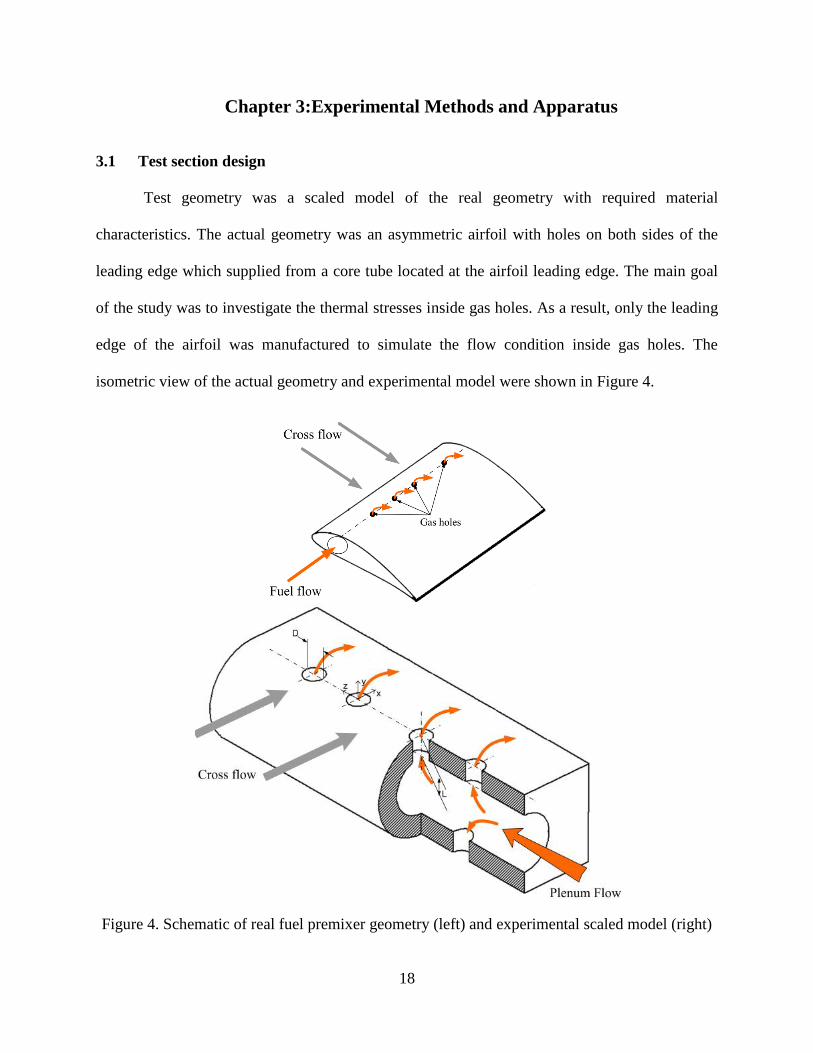
Test geometry was a scaled model of the real geometry with required material
characteristics. The actual geometry was an asymmetric airfoil with holes on both sides of the
leading edge which supplied from a core tube located at the airfoil leading edge. The main goal
of the study was to investigate the thermal stresses inside gas holes. As a result, only the leading
edge of the airfoil was manufactured to simulate the flow condition inside gas holes. The
isometric view of the actual geometry and experimental model were shown in Figure 4.
Figure 4. Schematic of real fuel premixer geometry (left) and experimental scaled model (right)

19
The test model was located inside a wind-tunnel to maintain the velocity ratio between jet
flow and cross flow. The model was extended four times the gas hole diameter along the cross
flow to eliminate vortex shedding effect at the backside of the model. The model scale up was
based on the Reynolds number and blowing ratios. The Reynolds number inside model gas holes
and the plenum was kept same as Reynolds number inside actual geometry gas holes and feed
tube.
The gas hole length to its diameter ratio was one and the overall size of model was
840mm (long side) by 300mm (along cross flow) by 250mm. The model was made of two halves
for ease in fabrication and instrumentation. The test section was made out of black Acetal for
optical purposes with thermal conductivity of 0.3 W/m-K (49)to satisfy semi-infinite body heat
conduction assumption for heat transfer measurement. Figure 5 shows the different components
on the test section.
Figure 5. Test section components
20
As shown in Figure 5. Test section components, the high pressure airline is connected to
the duct adapter. The duct adapter is a diffuser that changes area from 3” diameter pipe to a 6”
diameter plenum. The plenum extension is a 12” straight pipe to maintain the plenum modeled
length and provide the right velocity profile upstream the first gas hole. The plenum flow turns
into gas holes and ejects into the cross flow. Ten long bolts hold two halves of the test section
tightly through indicated bolt holes in Figure 5. Test section components. All gaps between the
model halves and plenum extension are sealed by silicon paste. Two small pressure tap holes
were located at both upstream and downstream sides of each gas hole entrance, inside the
plenum. Therefore, the pressure variation along the plenum can be monitored at both sides of gas
holes. The tiny channels at the back side of tap holes were designed for pressure measurement
tubing to prevent test section surface protrusion.
In Table 1 Operating condition and sizes for real geometry and scaled model, real
geometry and scaled up geometry sizes and operating conditions are presented. The gas hole and
plenum diameters are presented in millimeter. The flowing gas properties were not kept constant
between real geometry and scaled model due to the practical limitations. Also, the flow pressure
inside the real geometry was ten times the test model working pressure.
The main difference in flow structure between the real geometry and scaled model was
the compressibility. The Mach number inside the gas holes for the real geometry was in the
compressible situation while the Mach number inside scaled gas holes was in the incompressible
side. However, because of the experimental measurement devices limitation matching the Mach
number inside gas holes was not possible and compressibility effects inside gas holes was
neglected. The Reynolds number inside the gas holes of real geometry and test model were
perfectly matched. The difference between Reynolds numbers inside real and scaled plenum was
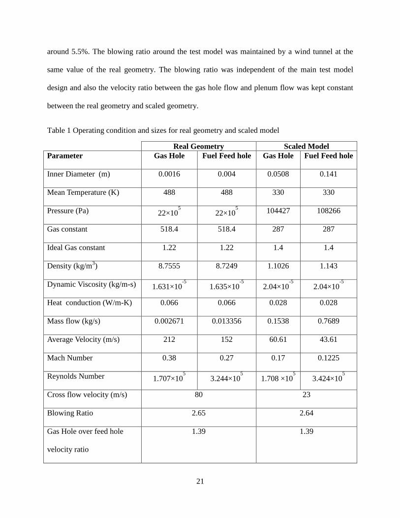
21
around 5.5%. The blowing ratio around the test model was maintained by a wind tunnel at the
same value of the real geometry. The blowing ratio was independent of the main test model
design and also the velocity ratio between the gas hole flow and plenum flow was kept constant
between the real geometry and scaled geometry.
Table 1 Operating condition and sizes for real geometry and scaled model
Real Geometry Scaled Model
Parameter Gas Hole Fuel Feed hole Gas Hole Fuel Feed hole
Inner Diameter (m) 0.0016 0.004 0.0508 0.141
Mean Temperature (K) 488 488 330 330
Pressure (Pa) 22×105 22×10
5 104427 108266
Gas constant 518.4 518.4 287 287
Ideal Gas constant 1.22 1.22 1.4 1.4
Density (kg/m3) 8.7555 8.7249 1.1026 1.143
Dynamic Viscosity (kg/m-s) 1.631×10⁻⁵
1.635×10⁻⁵
2.04×10⁻⁵
2.04×10⁻⁵
Heat conduction (W/m-K) 0.066 0.066 0.028 0.028
Mass flow (kg/s) 0.002671 0.013356 0.1538 0.7689
Average Velocity (m/s) 212 152 60.61 43.61
Mach Number 0.38 0.27 0.17 0.1225
Reynolds Number 1.707×10⁵ 3.244×10
5 1.708 ×10
5 3.424×10
5
Cross flow velocity (m/s) 80 23
Blowing Ratio 2.65 2.64
Gas Hole over feed hole
velocity ratio
1.39 1.39

22
The test section had four gas holes at one side and three gas holes at the other side.
However at each time, 5 gas holes out of the total 7 holes were open and four different
configurations of these holes were studied. These four configurations were ordered by industry.
Figure 6 presents the different arrangements of gas holes along the plenum channel.
Figure 6. Different gas holes arrangements along the plenum channel
3.1.1 Baffled test model
Moreover, to manipulate the heat transfer coefficient distribution inside gas holes,
straight baffles with different height were located inside the plenum. The straight baffles height
and distance from each gas hole exit was investigated numerically and validated experimentally.
Straight baffles were made out of 1.5 mm thick sheet metal to reach the plenum flow temperature
very fast. The baffles were attached to the plenum wall from the baffle base by two tapered head
plastic bolts at the same thermal conductivity as test model. Figure 7 shows the baffle shape and
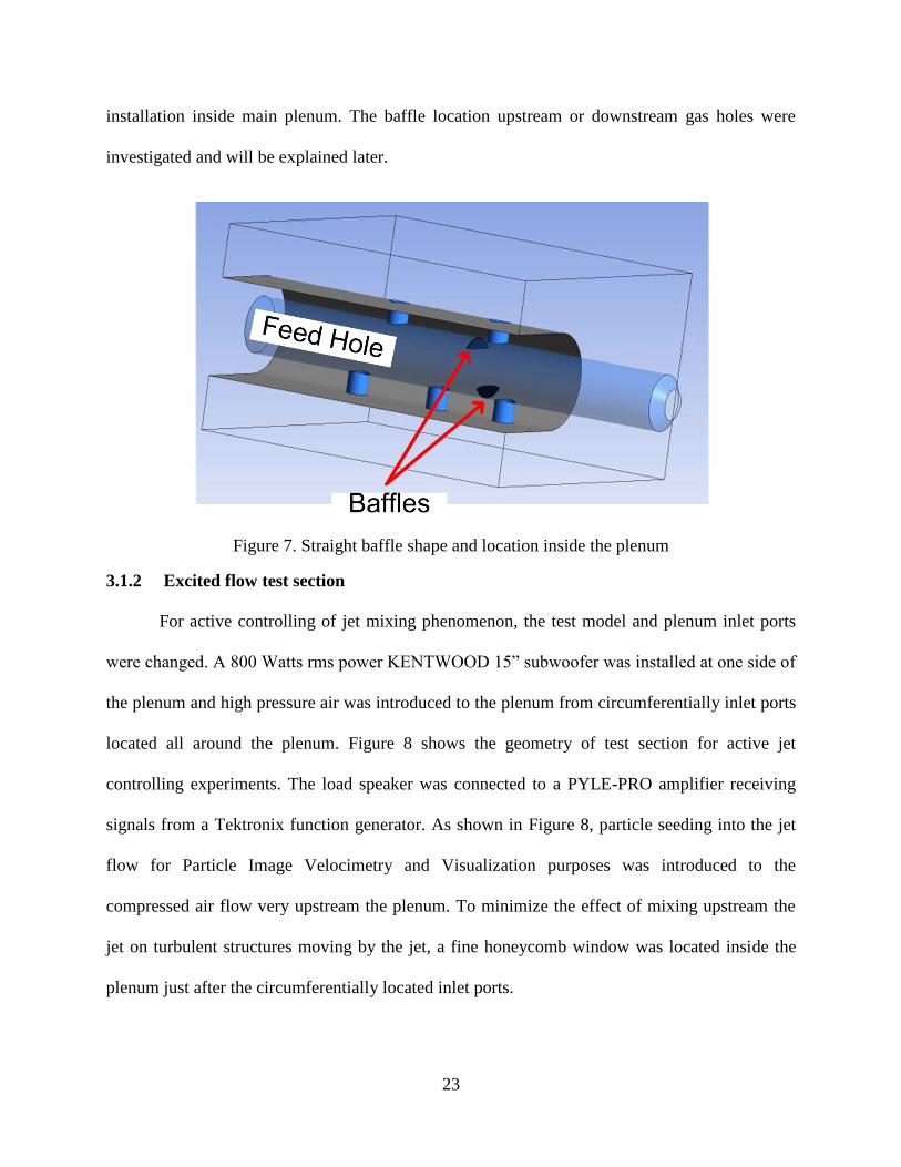
23
installation inside main plenum. The baffle location upstream or downstream gas holes were
investigated and will be explained later.
Figure 7. Straight baffle shape and location inside the plenum
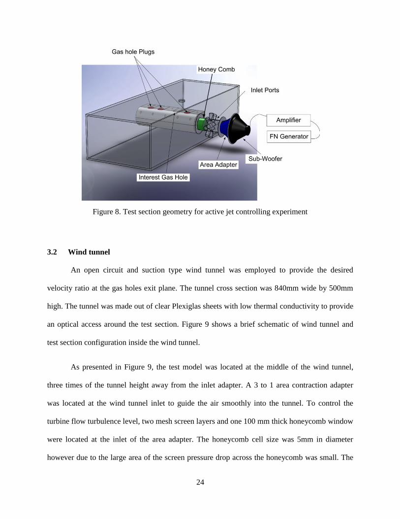
3.1.2 Excited flow test section
For active controlling of jet mixing phenomenon, the test model and plenum inlet ports
were changed. A 800 Watts rms power KENTWOOD 15” subwoofer was installed at one side of
the plenum and high pressure air was introduced to the plenum from circumferentially inlet ports
located all around the plenum. Figure 8 shows the geometry of test section for active jet
controlling experiments. The load speaker was connected to a PYLE-PRO amplifier receiving
signals from a Tektronix function generator. As shown in Figure 8, particle seeding into the jet
flow for Particle Image Velocimetry and Visualization purposes was introduced to the
compressed air flow very upstream the plenum. To minimize the effect of mixing upstream the
jet on turbulent structures moving by the jet, a fine honeycomb window was located inside the
plenum just after the circumferentially located inlet ports.
24
Figure 8. Test section geometry for active jet controlling experiment
3.2 Wind tunnel
An open circuit and suction type wind tunnel was employed to provide the desired
velocity ratio at the gas holes exit plane. The tunnel cross section was 840mm wide by 500mm
high. The tunnel was made out of clear Plexiglas sheets with low thermal conductivity to provide
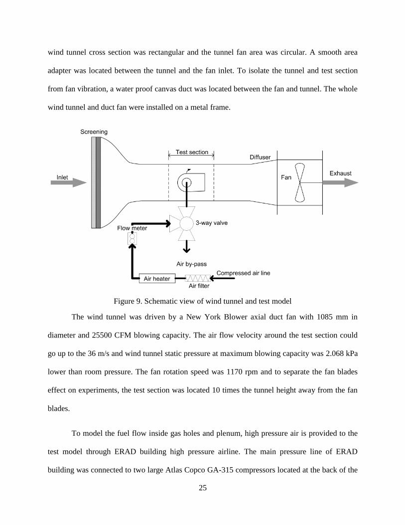
an optical access around the test section. Figure 9 shows a brief schematic of wind tunnel and
test section configuration inside the wind tunnel.
As presented in Figure 9, the test model was located at the middle of the wind tunnel,
three times of the tunnel height away from the inlet adapter. A 3 to 1 area contraction adapter
was located at the wind tunnel inlet to guide the air smoothly into the tunnel. To control the
turbine flow turbulence level, two mesh screen layers and one 100 mm thick honeycomb window
were located at the inlet of the area adapter. The honeycomb cell size was 5mm in diameter
however due to the large area of the screen pressure drop across the honeycomb was small. The
25
wind tunnel cross section was rectangular and the tunnel fan area was circular. A smooth area
adapter was located between the tunnel and the fan inlet. To isolate the tunnel and test section
from fan vibration, a water proof canvas duct was located between the fan and tunnel. The whole
wind tunnel and duct fan were installed on a metal frame.
Figure 9. Schematic view of wind tunnel and test model
The wind tunnel was driven by a New York Blower axial duct fan with 1085 mm in
diameter and 25500 CFM blowing capacity. The air flow velocity around the test section could
go up to the 36 m/s and wind tunnel static pressure at maximum blowing capacity was 2.068 kPa
lower than room pressure. The fan rotation speed was 1170 rpm and to separate the fan blades
effect on experiments, the test section was located 10 times the tunnel height away from the fan
blades.
To model the fuel flow inside gas holes and plenum, high pressure air is provided to the
test model through ERAD building high pressure airline. The main pressure line of ERAD
building was connected to two large Atlas Copco GA-315 compressors located at the back of the
26
ERAD building. Each compressor generated 1399 CFM at 157 PSI to support the wide range of
required mass flow rates. The compressed air went through two auto drain Wilkerson F35 series
particulate filter. The filters were taking water particles and rust out of airline and provided test
section by a clear and dry air. The main compressed airline of ERAD building was provided by
three 50.8 mm valve into the laboratory. However, reaching the design Reynolds number was not
possible from one valve due to the chocking effect. Therefore, two 50.8 mm valves were
connected to one 76.2 mm pipe line and compressed air was introduced to the test section
through a 76.2 mm flexible rubber pipe.
Each 50.8 mm pipe line was connected to a particulate filter and a coil heater
respectively. The coil heaters were manufactured by InfinityFluids. One heater had 20,000 Watts
capacity while the other heater was 6000 Watts. By using 26,000 Watts heating power, the
compressed air line temperature could rise around 50oC above the ambient temperature required
for heat transfer coefficient measurements. Downstream the heater, air was passed through a
flow meter at each branch. One flow meter is a CDI-5400 thermal mass flow meter calibrated at
the experimental temperature range. The other flow meter was a Flowmetrics, Inc turbine flow
meter model FM-48NT measuring actual air volumetric flow rate at each pressure and
temperature. So, a T-type thermocouple and a pressure gauge were installed upstream the flow
meter for calculating the flow density during experiments.
3.3 Heat transfer coefficient calculation by wall temperature
For heat transfer measurement inside gas holes the transient heat conduction test was
performed. The one dimensional heat conduction equation was solved inside the solid body by
semi infinite heat conduction boundary conditions. By this assumption, the heat transfer
27
coefficient (HTC) on wall is related to the instantaneous wall and air temperature for different
times by the following equation (1).
Equation 1
Tw −T0
T∞−T0 = 1 − exp
h2αt
k2 erfc h αt
k
In this equation α is thermal diffusivity and k is the thermal conductivity of test geometry
material. “t” is the time from the beginning of the test, Tw is the wall temperature at each time, T0
is the wall initial temperature and 𝑇∞ is the instantaneous flow temperature. The flow
temperature is measured by T-type thermocouples placed inside the hole. Thermocouple data
was recorded by a national instrument SCXI-1600 data acquisition module and connected to PC
by a USB cord. Before running the test, geometry was kept at a uniform temperature. Three
thermocouples were installed on different points on the test geometry to ensure temperature
uniformity all around the test model body. The plenum flow was heated up to the desired
temperature by inline heaters. The tunnel fan was running at a steady velocity one minute before
running the test. A LABVIEW code was running prior to starting the test to record thermocouple
temperatures.
For the transient test, a sudden change in flow temperature was required. Therefore, a
76.2 mm three way valve was located before the compressed air enters into the test section as
shown in Figure 9. Before running the test, heated air flow was bypassed by the valve until the
flow temperature reached the desired temperature. Then, the valve was suddenly changed the air
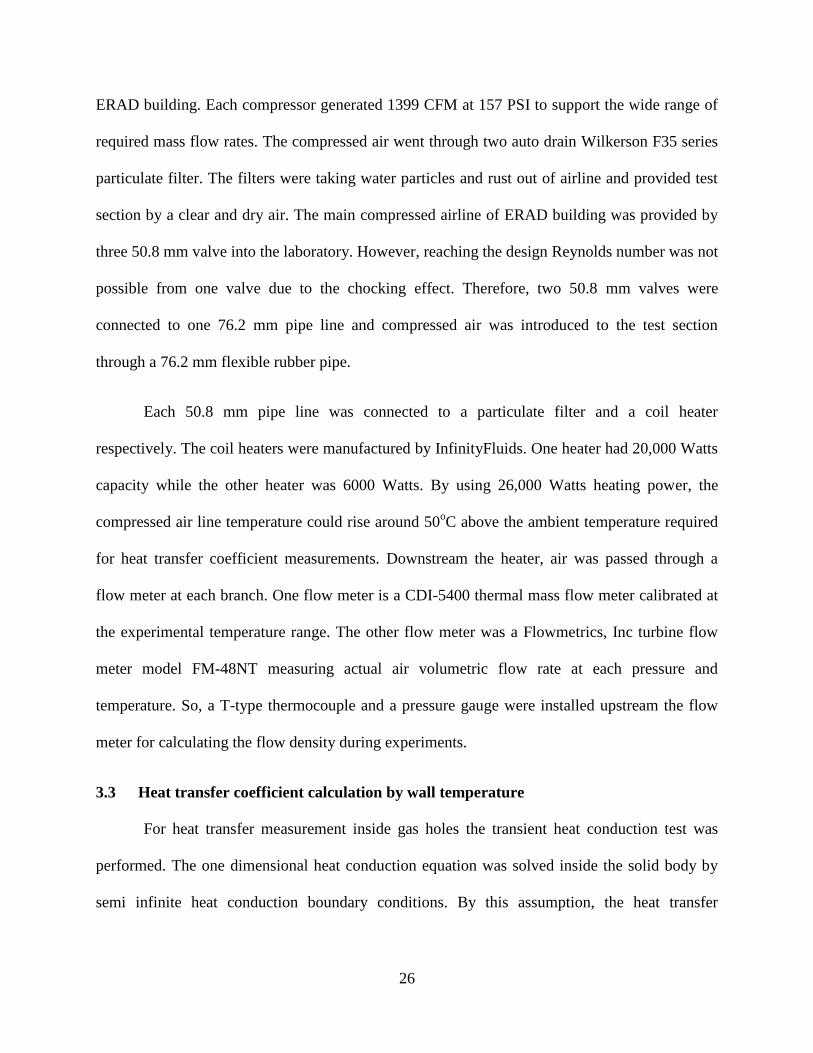
pass and hot air flow passed through test section and gas holes. Figure 10, presents the air flow
temperature variation inside gas holes during experiments.
28
Figure 10. Air temperature variation during experiments inside gas holes
As presented in Figure.10, the temperature rise during a test run was not sharp enough for
transient heat transfer test and the Duhamel integration was applied to Equation 1 to correct the
delay in temperature rise. The bulk airflow temperature inside gas holes was measured by a
0.025mm thick T-type thermocouple. The thermocouples were connected to PC through a SCXI-
1000 National instrument data acquisition board. The thermocouple module was connected to PC
by a USB cable and thermocouple signals were transferred and stored in an excel spreadsheet by
LABVIEW 8.6.
3.4 Temperature measurement inside gas holes
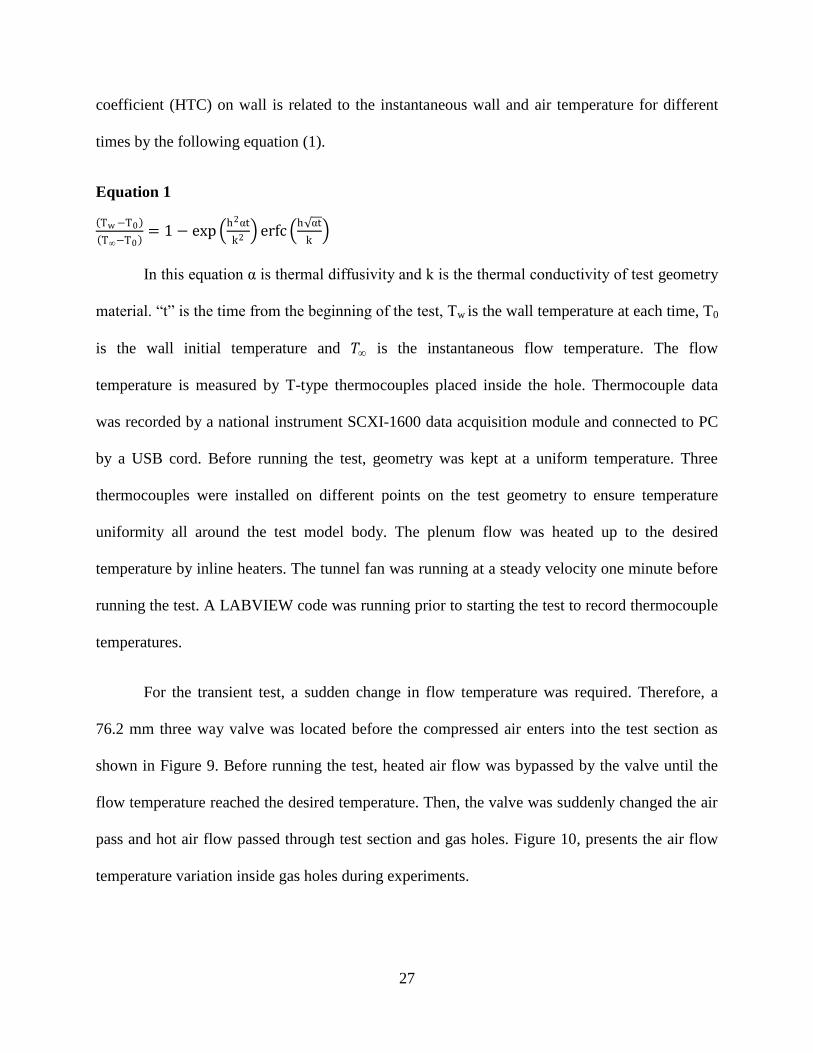
3.4.1 Infra red camera thermography
To measure the wall temperature inside gas holes, a FLIR-SC high speed infrared camera
was used. The camera was located above the test section at an angle to look inside gas holes.
29
The camera inclination angle and distance from the gas hole wall was selected based on the
camera calibration chart. The camera angle in respect to vertical line was 55o and all temperature
calibrations were performed at this angle. Figure 11, presents the configuration of Infrared
camera looking inside gas holes from outside.
Figure 11. Infrared camera location above the wind tunnel looking into gas holes
The infrared camera calibration was performed by ExaminIR software. For the
calibration process, a small heating screen was attached to the backside of a thin black Acetal
piece and located at the same distance and angle of a gas hole surface. Due to the low
transparency factor of Plexiglas sheet for Infrared light (3-5 μm wavelengths) a Zinc-Selenide
(Zn-Se) window was installed above the wind tunnel for optical access into the gas holes with
transparency factor of 97%. Figure 12 shows the Zinc-Selenide window employed during heat
transfer measurement experiments. The Zn-Se window was located inside a portable mount
made out of Plexiglas because the window was extremely fragile.
30
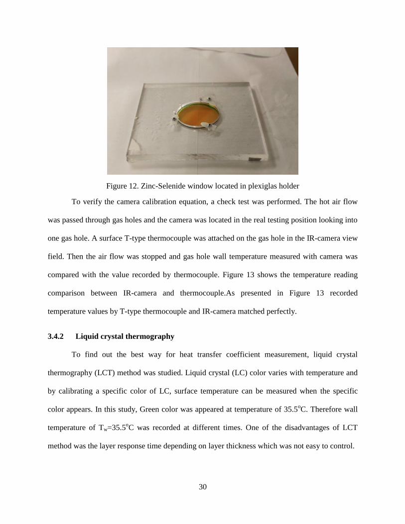
Figure 12. Zinc-Selenide window located in plexiglas holder
To verify the camera calibration equation, a check test was performed. The hot air flow
was passed through gas holes and the camera was located in the real testing position looking into
one gas hole. A surface T-type thermocouple was attached on the gas hole in the IR-camera view
field. Then the air flow was stopped and gas hole wall temperature measured with camera was
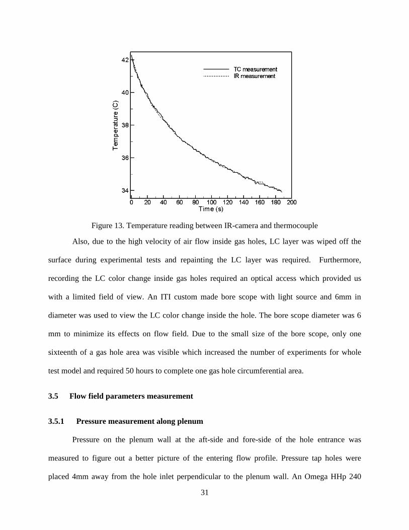
compared with the value recorded by thermocouple. Figure 13 shows the temperature reading
comparison between IR-camera and thermocouple.As presented in Figure 13 recorded
temperature values by T-type thermocouple and IR-camera matched perfectly.
3.4.2 Liquid crystal thermography
To find out the best way for heat transfer coefficient measurement, liquid crystal
thermography (LCT) method was studied. Liquid crystal (LC) color varies with temperature and
by calibrating a specific color of LC, surface temperature can be measured when the specific
color appears. In this study, Green color was appeared at temperature of 35.5oC. Therefore wall
temperature of Tw=35.5oC was recorded at different times. One of the disadvantages of LCT
method was the layer response time depending on layer thickness which was not easy to control.
31
Figure 13. Temperature reading between IR-camera and thermocouple
Also, due to the high velocity of air flow inside gas holes, LC layer was wiped off the
surface during experimental tests and repainting the LC layer was required. Furthermore,
recording the LC color change inside gas holes required an optical access which provided us
with a limited field of view. An ITI custom made bore scope with light source and 6mm in
diameter was used to view the LC color change inside the hole. The bore scope diameter was 6
mm to minimize its effects on flow field. Due to the small size of the bore scope, only one
sixteenth of a gas hole area was visible which increased the number of experiments for whole
test model and required 50 hours to complete one gas hole circumferential area.
3.5 Flow field parameters measurement
3.5.1 Pressure measurement along plenum
Pressure on the plenum wall at the aft-side and fore-side of the hole entrance was
measured to figure out a better picture of the entering flow profile. Pressure tap holes were
placed 4mm away from the hole inlet perpendicular to the plenum wall. An Omega HHp 240

32
pressure module was employed to record averaged pressure values during one minute at each
location. Figure 14 shows a schematic of pressure tap hole locations at both sides on a gas hole.
Figure 14. Schematic of pressure tap holes locations
3.5.2 Velocity measurement inside gas holes by Pitot static tube
Velocity distribution inside gas holes had the most significant effect on heat transfer
coefficient on gas holes wall. The velocity profile inside each hole was measured by a fine Pitot
static tube with 1mm in diameter of probe at the middle plane of each hole. The velocity values
were recorded at every 6mm along the diagonal lines “I” and “C” as shown in Figure.14. Time
averaged pressure values during one minute with 10Hz frequency was used to calculate mean
velocity at each location along diagonal lines. Figure 15 shows data recording locations inside
the hole in respect to plenum flow direction and tunnel flows. As shown in Figure.15, line “I” is
along the plenum and main flow complexities were happened along line “I”. The “C” line was a
cross diagonal line and velocity profile should show a sort of symmetry at this plane.
33
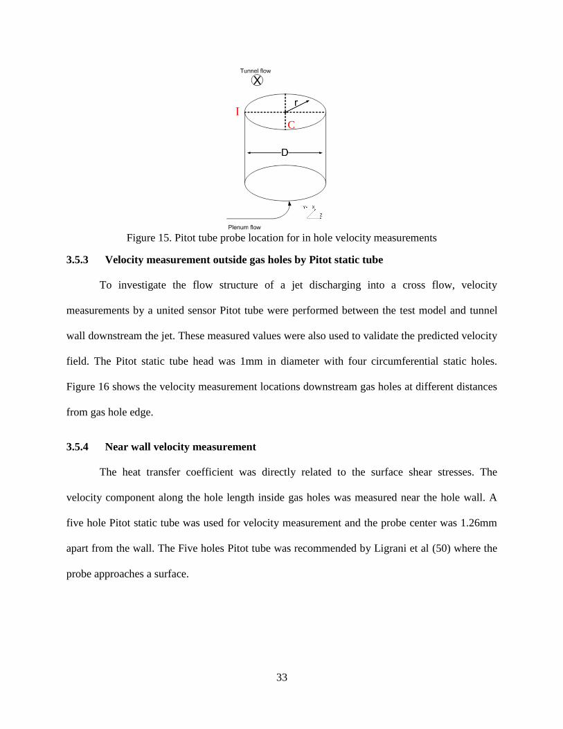
Figure 15. Pitot tube probe location for in hole velocity measurements
3.5.3 Velocity measurement outside gas holes by Pitot static tube
To investigate the flow structure of a jet discharging into a cross flow, velocity
measurements by a united sensor Pitot tube were performed between the test model and tunnel
wall downstream the jet. These measured values were also used to validate the predicted velocity
field. The Pitot static tube head was 1mm in diameter with four circumferential static holes.
Figure 16 shows the velocity measurement locations downstream gas holes at different distances
from gas hole edge.
3.5.4 Near wall velocity measurement
The heat transfer coefficient was directly related to the surface shear stresses. The
velocity component along the hole length inside gas holes was measured near the hole wall. A
five hole Pitot static tube was used for velocity measurement and the probe center was 1.26mm
apart from the wall. The Five holes Pitot tube was recommended by Ligrani et al (50) where the
probe approaches a surface.
C
34
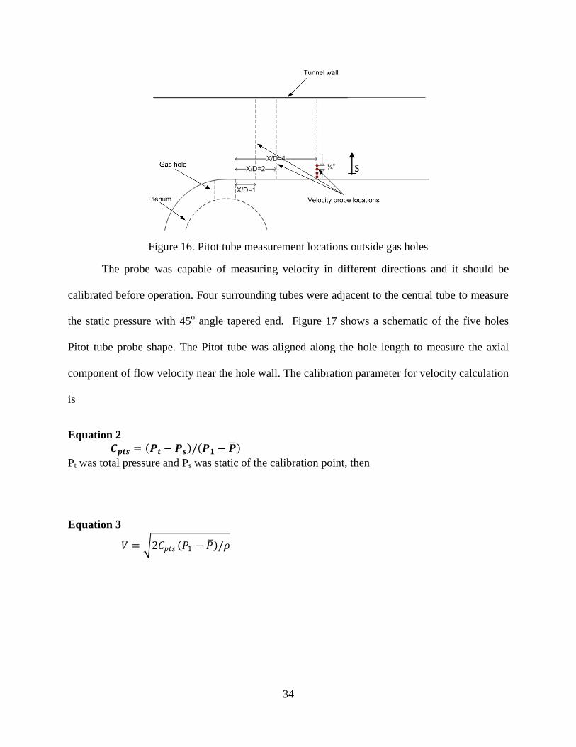
Figure 16. Pitot tube measurement locations outside gas holes
The probe was capable of measuring velocity in different directions and it should be
calibrated before operation. Four surrounding tubes were adjacent to the central tube to measure
the static pressure with 45o angle tapered end. Figure 17 shows a schematic of the five holes
Pitot tube probe shape. The Pitot tube was aligned along the hole length to measure the axial
component of flow velocity near the hole wall. The calibration parameter for velocity calculation
is
Equation 2
𝑪𝒑𝒕𝒔 = 𝑷𝒕 − 𝑷𝒔 / 𝑷𝟏 − 𝑷
Pt was total pressure and Ps was static of the calibration point, then
Equation 3
𝑉 = 2𝐶𝑝𝑡𝑠 𝑃1 − 𝑃 /𝜌
S
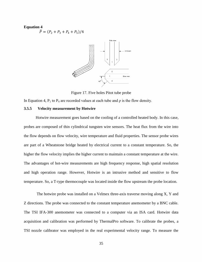
35
Equation 4
𝑃 = 𝑃2 + 𝑃3 + 𝑃4 + 𝑃5 /4
Figure 17. Five holes Pitot tube probe
In Equation 4, P1 to P4 are recorded values at each tube and ρ is the flow density.
3.5.5 Velocity measurement by Hotwire
Hotwire measurement goes based on the cooling of a controlled heated body. In this case,
probes are composed of thin cylindrical tungsten wire sensors. The heat flux from the wire into
the flow depends on flow velocity, wire temperature and fluid properties. The sensor probe wires
are part of a Wheatstone bridge heated by electrical current to a constant temperature. So, the
higher the flow velocity implies the higher current to maintain a constant temperature at the wire.
The advantages of hot-wire measurements are high frequency response, high spatial resolution
and high operation range. However, Hotwire is an intrusive method and sensitive to flow
temperature. So, a T-type thermocouple was located inside the flow upstream the probe location.
The hotwire probe was installed on a Velmex three-axis traverse moving along X, Y and
Z directions. The probe was connected to the constant temperature anemometer by a BNC cable.
The TSI IFA-300 anemometer was connected to a computer via an ISA card. Hotwire data
acquisition and calibration was performed by ThermalPro software. To calibrate the probes, a
TSI nozzle calibrator was employed in the real experimental velocity range. To measure the
36
velocity magnitude and fluctuations, a single probe TSI-1210 was employed. The probe
calibration gain and offset was modified based on the velocity range and air flow temperature.
The ThermalPro software fitted a power function to the calibration values and the calibration
equation was generated by the software. During the hotwire a measurement, air flow temperature
was kept constant same as the calibration jet temperature.
3.5.6 Particle Image Velocimetry
For better understanding of jet trajectory and mixing phenomenon, a Particle Image
Velocimetry (PIV) technique was employed. For visualization injection of a tracer into the jet
flow was required in order to reveal the velocity profile of jet mixing with the cross-flow. The
particle enriched jet flow was illuminated using a LASER sheet, and particle images were taken
using a digital camera looking perpendicularly to the LASER sheet. One visualization plane was
considered for this study, perpendicular to the bottom wall of the test section and parallel to the
cross flow direction (X-Y plane as shown in Figure.4).
Sub micron size olive oil particles were injected into the plenum flow for PIV
measurement. The particles were generated by an ATI TDA-4B aerosol generator. The olive oil
particles were introduced to the plenum flow upstream the inlet ports shown in Figure.8. The oil
particles were evenly distributed among eight incoming inlet ports and during the flow mixing
upstream the honeycomb screen inside the plenum, a homogeneous aerosol mixture was made.
Because of the non-toxic characteristic of olive oil, extra ventilation systems, goggles and heavy
duty latex gloves were not required just respiratory masks. However, the main disadvantages of
submicron olive oil particles was the particle sizes which was perfect to follow the turbulence
structures but difficult to view.
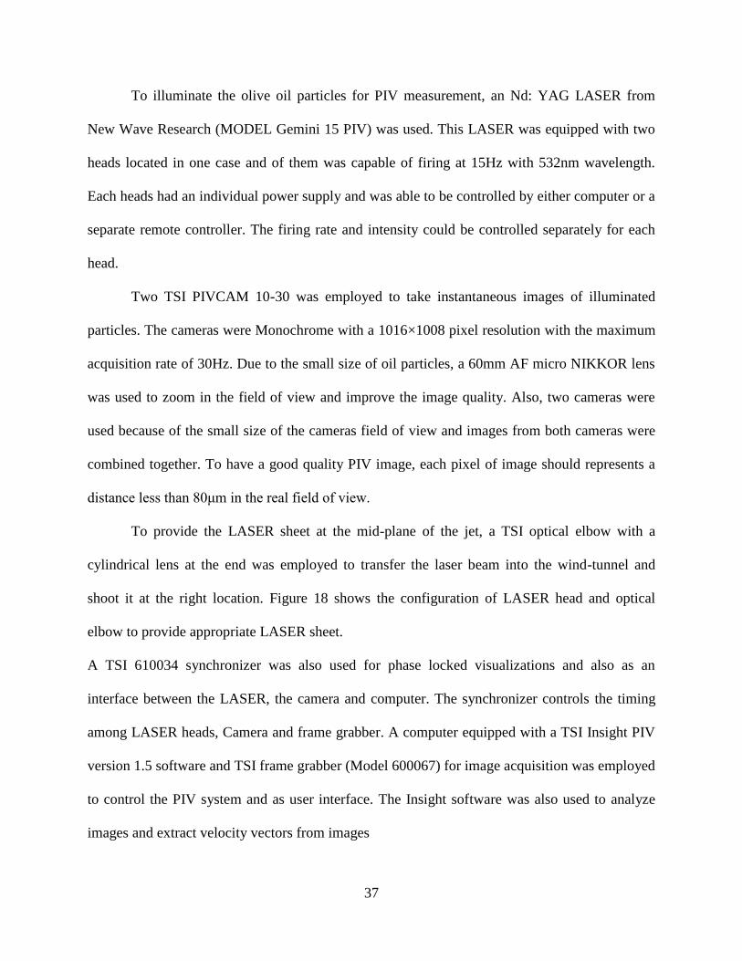
37
To illuminate the olive oil particles for PIV measurement, an Nd: YAG LASER from
New Wave Research (MODEL Gemini 15 PIV) was used. This LASER was equipped with two
heads located in one case and of them was capable of firing at 15Hz with 532nm wavelength.
Each heads had an individual power supply and was able to be controlled by either computer or a
separate remote controller. The firing rate and intensity could be controlled separately for each
head.
Two TSI PIVCAM 10-30 was employed to take instantaneous images of illuminated
particles. The cameras were Monochrome with a 1016×1008 pixel resolution with the maximum
acquisition rate of 30Hz. Due to the small size of oil particles, a 60mm AF micro NIKKOR lens
was used to zoom in the field of view and improve the image quality. Also, two cameras were
used because of the small size of the cameras field of view and images from both cameras were
combined together. To have a good quality PIV image, each pixel of image should represents a
distance less than 80μm in the real field of view.
To provide the LASER sheet at the mid-plane of the jet, a TSI optical elbow with a
cylindrical lens at the end was employed to transfer the laser beam into the wind-tunnel and
shoot it at the right location. Figure 18 shows the configuration of LASER head and optical
elbow to provide appropriate LASER sheet.
A TSI 610034 synchronizer was also used for phase locked visualizations and also as an
interface between the LASER, the camera and computer. The synchronizer controls the timing
among LASER heads, Camera and frame grabber. A computer equipped with a TSI Insight PIV
version 1.5 software and TSI frame grabber (Model 600067) for image acquisition was employed
to control the PIV system and as user interface. The Insight software was also used to analyze
images and extract velocity vectors from images

38
Figure 18. Optical configuration of laser head, optical elbow and PIV cameras
3.5.7 High speed flow visualization
Due to the low frequency of PIV system, tracking the seeded particles moving by
turbulence structures was impossible. The natural frequency of turbulent structures moving by
the vertical jet were very high and employing high speed imaging was necessary. Therefore, a
Photron SA3-120K monochrome high speed camera was employed. A UVI camera intensifier
was installed in fron of the Photron camera to improve the intensity of the images. To track the
high speed structures moving by the flow, one constant laser sheet provided by a 175mW solid
state LASER was located at the mid-plane of the target gas hole vertically along the tunnel. Also,
a horizontal LASER sheet was placed above the gas hole exit plane one gas hole diameter from
the jet exit plane. The optics employed for this visualization are same as the PIV system and the
optical elbow with a spherical lens was not replaced. The high speed camera was connected to
39
PC via an Ethernet cable and controlled by PFV ver.323 software. The image recording data
acquisition rate could go up to 120K Hz but in this project, data recording rate of 4000 Hz was
adequate. The camera intensifier gain value was dependent on the intensifier distance from
LASER sheet. So, the gain value for the vertical LASER sheet was 73 and 65 for the horizontal
sheet. Figure 19 presents the LASER sheet location in respect to the jet and Photron camera. As
shown, the image intensifier is located in front of the camera and a focusing was required
between the intensifier and camera.
Figure 19 Vertical LASER sheet and Photron camera configuration
The flow visualization images show instantaneous jet shape every 0.00025 of a second.
Therefore, to investigate the jet overall behavior in a long duration, visualization images were
intensity averaged. For this averaging process, the LASER sheet power and camera configuration
for all different test cases were kept constant. The totals of 4850 images were averaged to
provide the jet mean trajectory during time. To investigate the effect of number of averaged
images on the averaging results, mean trajectory with different averaged images are presented in
Figure 20 for both vertical and horizontal planes. The horizontal plane images were captured at
the location indicated by red dashed line in Figure 20, top row.
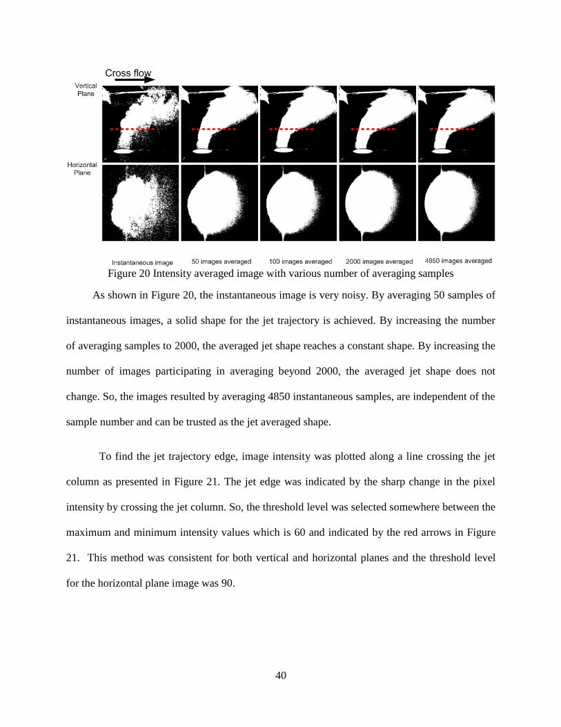
40
Figure 20 Intensity averaged image with various number of averaging samples
As shown in Figure 20, the instantaneous image is very noisy. By averaging 50 samples of
instantaneous images, a solid shape for the jet trajectory is achieved. By increasing the number
of averaging samples to 2000, the averaged jet shape reaches a constant shape. By increasing the
number of images participating in averaging beyond 2000, the averaged jet shape does not
change. So, the images resulted by averaging 4850 instantaneous samples, are independent of the
sample number and can be trusted as the jet averaged shape.
To find the jet trajectory edge, image intensity was plotted along a line crossing the jet
column as presented in Figure 21. The jet edge was indicated by the sharp change in the pixel
intensity by crossing the jet column. So, the threshold level was selected somewhere between the
maximum and minimum intensity values which is 60 and indicated by the red arrows in Figure
21. This method was consistent for both vertical and horizontal planes and the threshold level
for the horizontal plane image was 90.

41
Figure 21 Pixel intensity along red dotted line
3.6 Error analysis of experimental methods
3.6.1 Different heat transfer measurement methods
To choose the right method to measure heat transfer coefficient on gas hole walls, three
different experimental methods were investigated and compared. Infra red thermography on gas
holes wall, liquid crystal thermography and wall temperature measurement with surface
thermocouples were compared. Heat transfer coefficient resulted from three discussed methods
was compared in Figure 22. The values were extracted inside gas hole 4 of case-A shown in
Figure.6 along a line from hole inlet to exit on the aft-side. Trend of HTC with liquid crystal
thermography was similar to that of Infra red thermography. But, HTCs resulted by
thermocouples do not follow the same trend as liquid crystal and infra-red results. The measured
HTC value at the gas hole inlet by thermocouple was very close to HTC recorded by other
methods due to the thin boundary layer at that region. By moving down the gas hole, the
boundary layer thickened and thermocouple was measuring a value between wall temperature
and main flow. The Liquid crystal and Infra red thermography recorded similar values but as
explained in section 3.4.1, employing infra red thermography was applicable
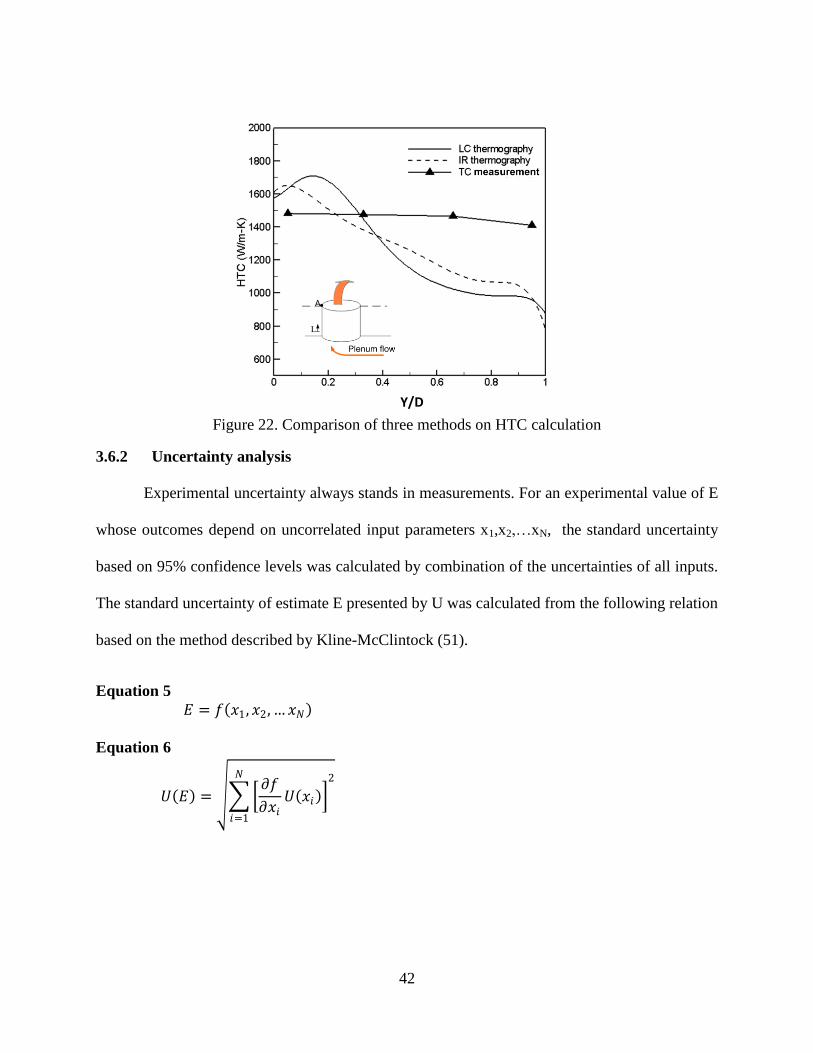
42
Figure 22. Comparison of three methods on HTC calculation
3.6.2 Uncertainty analysis
Experimental uncertainty always stands in measurements. For an experimental value of E
whose outcomes depend on uncorrelated input parameters x1,x2,…xN, the standard uncertainty
based on 95% confidence levels was calculated by combination of the uncertainties of all inputs.
The standard uncertainty of estimate E presented by U was calculated from the following relation
based on the method described by Kline-McClintock (51).
Equation 5
𝐸 = 𝑓 𝑥1, 𝑥2,…𝑥𝑁
Equation 6
𝑈 𝐸 = 𝜕𝑓
𝜕𝑥𝑖𝑈 𝑥𝑖
2𝑁
𝑖=1
Y/D
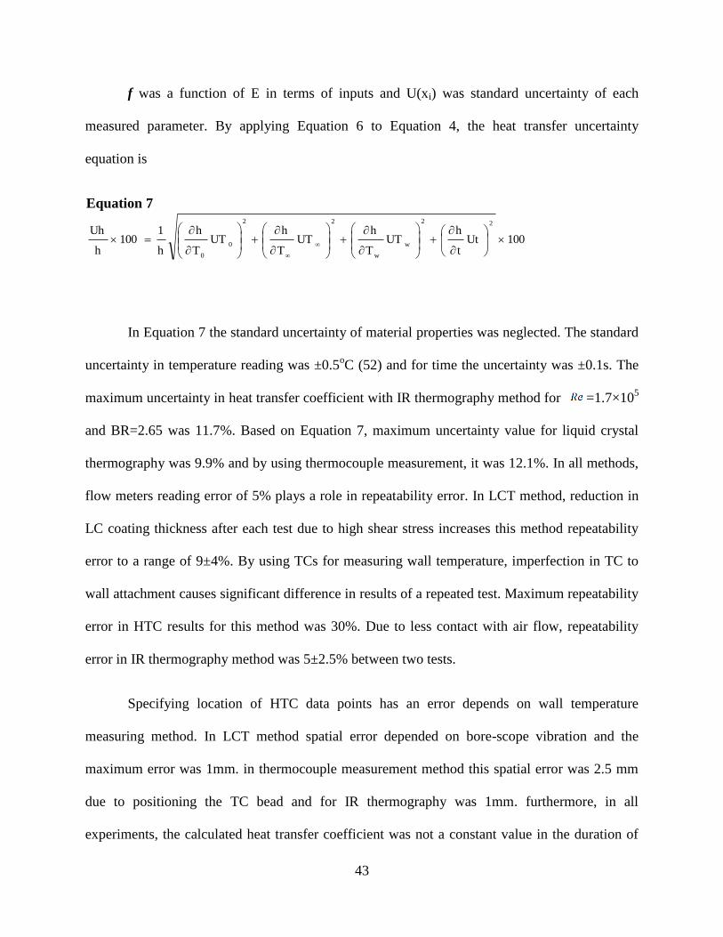
43
f was a function of E in terms of inputs and U(xi) was standard uncertainty of each
measured parameter. By applying Equation 6 to Equation 4, the heat transfer uncertainty
equation is
Equation 7
100Utt
hUT
T
hUT
T
hUT
T
h
h
1100
h
Uh22
w
w
22
0
0
In Equation 7 the standard uncertainty of material properties was neglected. The standard
uncertainty in temperature reading was ±0.5oC (52) and for time the uncertainty was ±0.1s. The
maximum uncertainty in heat transfer coefficient with IR thermography method for =1.7×10⁵
and BR=2.65 was 11.7%. Based on Equation 7, maximum uncertainty value for liquid crystal
thermography was 9.9% and by using thermocouple measurement, it was 12.1%. In all methods,
flow meters reading error of 5% plays a role in repeatability error. In LCT method, reduction in
LC coating thickness after each test due to high shear stress increases this method repeatability
error to a range of 9±4%. By using TCs for measuring wall temperature, imperfection in TC to
wall attachment causes significant difference in results of a repeated test. Maximum repeatability
error in HTC results for this method was 30%. Due to less contact with air flow, repeatability
error in IR thermography method was 5±2.5% between two tests.
Specifying location of HTC data points has an error depends on wall temperature
measuring method. In LCT method spatial error depended on bore-scope vibration and the
maximum error was 1mm. in thermocouple measurement method this spatial error was 2.5 mm
due to positioning the TC bead and for IR thermography was 1mm. furthermore, in all
experiments, the calculated heat transfer coefficient was not a constant value in the duration of

44
the test. At the beginning of the test, HTC value was very high. Then it decreases sharply in first
five seconds of the experiment and flatten to a steady value (53). Because of this, all HTC values
were calculated at t=30s where the HTC variation with time was small. Figure 23 shows the
variation of heat transfer coefficient with time near the hole inlet for gas hole 1.
Figure 23. Variation of measured HTC at two different locations inside gas hole 1 versus time

45
4 Chapter 4: Numerical Simulation
For improved understanding of flow structure inside the gas holes, numerical simulation
using the commercial software FLUENT 12.1 was employed. Incompressible momentum,
turbulence and energy equations in fluid flow were solved by finite volume method as equations
discretization scheme. To model the turbulence disturbances, high Reynolds number K-ε model
was applied. Hexahedral grid cells were generated using ANSYS-ICEM software in the flow
field.
4.1 Reynolds-averaged Navier-Stokes equations (RANS)
RANS methods are very convenient in turbulence flow modeling. One of the most
popular RANS models for simulating the industrial flow fields is K- ε method. Realizable K-ε is
a two equations RANS model which is valid for fully turbulent flows and has a reasonable
accuracy for wide range of industrial flows. This method was recommended for flows with
strong separation, strong streamline curvature and recirculation structures [FLUENT (54)]. For
realizable K-ε model, effects of wall boundaries on flow field were applied by different near wall
treatments. Near wall treatment selection depends strongly on flow structure and geometrical
complexities.
4.1.1 Flow simulation inside one gas hole
Simulating the flow field inside one gas hole was done with high Reynolds number
realizable k-ε model. This geometry consists of one gas hole and a portion of plenum and wind
tunnel. A schematic of flow domain and applied boundary conditions are shown in Figure 24.
This geometry was a simple model of one gas hole without the effect of neighboring holes. The
purpose of flow simulation in this geometry was for grid density analysis and near wall cell
adaptation. In this geometry, Cross flow and plenum flow boundaries were velocity inlet

46
boundary conditions and tunnel outlet was an outflow boundary condition with velocity vector
direction perpendicular to the boundary. All wall boundaries were satisfied no-slip condition on
the wall. The boundary layer forms on the wall and its growth was predicted by turbulence near
wall equations.
Figure 24. Schematic of one gas hole geometry with appropriate boundary conditions
In this geometry due to the flow complexity Non-equilibrium wall function was used as a
near wall treatment model. This model was recommended for flows with sudden changes on wall
boundaries, separation and impingement [FLUENT (54)]. In this model, the first grid point size
adjacent to the wall is set in a way that the turbulent viscous sub-layer locates inside the first cell.
To investigate the suitability of first cell size, wall Y+ value on the gas hole wall was monitored.
For Non-equilibrium wall function model Y+ value on the gas hole wall was kept between 30 to
100.
C ross flow
P lenum flow
Tunnel outle t
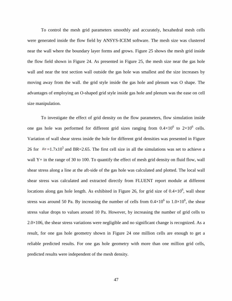
47
To control the mesh grid parameters smoothly and accurately, hexahedral mesh cells
were generated inside the flow field by ANSYS-ICEM software. The mesh size was clustered
near the wall where the boundary layer forms and grows. Figure 25 shows the mesh grid inside
the flow field shown in Figure 24. As presented in Figure 25, the mesh size near the gas hole
wall and near the test section wall outside the gas hole was smallest and the size increases by
moving away from the wall. the grid style inside the gas hole and plenum was O shape. The
advantages of employing an O-shaped grid style inside gas hole and plenum was the ease on cell
size manipulation.
To investigate the effect of grid density on the flow parameters, flow simulation inside
one gas hole was performed for different grid sizes ranging from 0.4×10⁶ to 2×10
6 cells.
Variation of wall shear stress inside the hole for different grid densities was presented in Figure
26 for =1.7x10⁵
and BR=2.65. The first cell size in all the simulations was set to achieve a
wall Y+ in the range of 30 to 100. To quantify the effect of mesh grid density on fluid flow, wall
shear stress along a line at the aft-side of the gas hole was calculated and plotted. The local wall
shear stress was calculated and extracted directly from FLUENT report module at different
locations along gas hole length. As exhibited in Figure 26, for grid size of 0.4×10⁶, wall shear
stress was around 50 Pa. By increasing the number of cells from 0.4×10⁶ to 1.0×10
6, the shear
stress value drops to values around 10 Pa. However, by increasing the number of grid cells to
2.0×10⁶, the shear stress variations were negligible and no significant change is recognized. As a
result, for one gas hole geometry shown in Figure 24 one million cells are enough to get a
reliable predicted results. For one gas hole geometry with more than one million grid cells,
predicted results were independent of the mesh density.
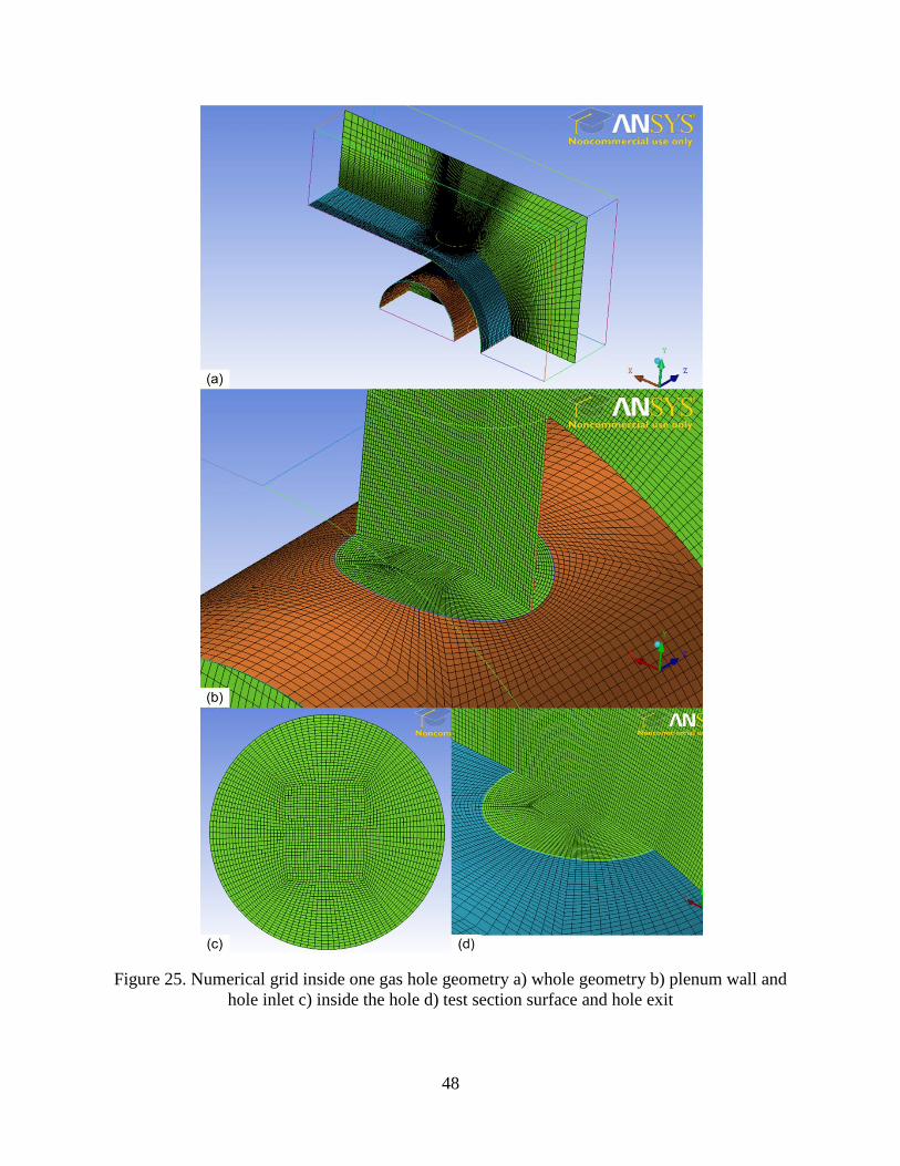
48
Figure 25. Numerical grid inside one gas hole geometry a) whole geometry b) plenum wall and
hole inlet c) inside the hole d) test section surface and hole exit
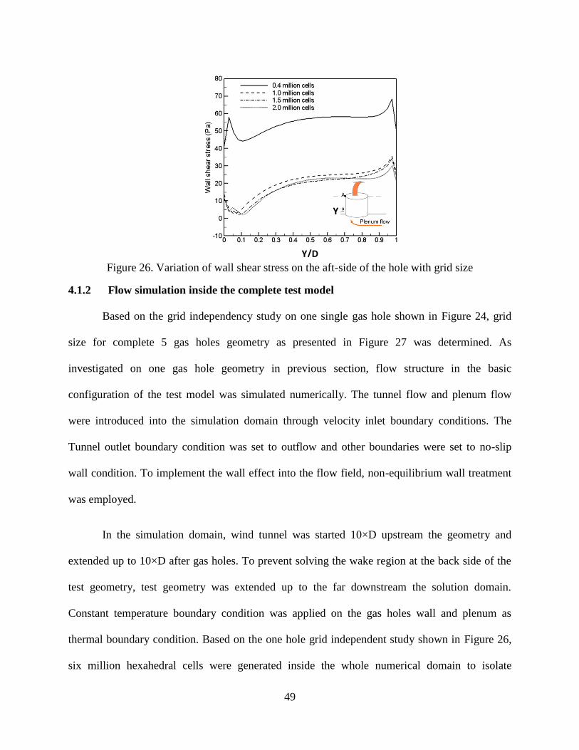
49
Figure 26. Variation of wall shear stress on the aft-side of the hole with grid size
4.1.2 Flow simulation inside the complete test model
Based on the grid independency study on one single gas hole shown in Figure 24, grid
size for complete 5 gas holes geometry as presented in Figure 27 was determined. As
investigated on one gas hole geometry in previous section, flow structure in the basic
configuration of the test model was simulated numerically. The tunnel flow and plenum flow
were introduced into the simulation domain through velocity inlet boundary conditions. The
Tunnel outlet boundary condition was set to outflow and other boundaries were set to no-slip
wall condition. To implement the wall effect into the flow field, non-equilibrium wall treatment
was employed.
In the simulation domain, wind tunnel was started 10×D upstream the geometry and
extended up to 10×D after gas holes. To prevent solving the wake region at the back side of the
test geometry, test geometry was extended up to the far downstream the solution domain.
Constant temperature boundary condition was applied on the gas holes wall and plenum as
thermal boundary condition. Based on the one hole grid independent study shown in Figure 26,
six million hexahedral cells were generated inside the whole numerical domain to isolate
Y/D
Y
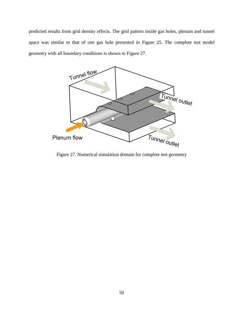
50
predicted results from grid density effects. The grid pattern inside gas holes, plenum and tunnel
space was similar to that of one gas hole presented in Figure 25. The complete test model
geometry with all boundary conditions is shown in Figure 27.
Figure 27. Numerical simulation domain for complete test geometry
51
5 Chapter 5: Results and Discussion
Results will be presented initially for the baseline configuration (labeled configuration A
in Figure 6), for a range of Reynolds numbers based on an estimated equi-distribution of flow
through each hole (𝑅𝑒 ) and for different blowing ratios BR, defined as the ratio of the gas-hole
velocity to the cross-flow velocity. Where noted in the text, a local hole-Reynolds number ReL
based on the local predicted mass flow rate through each hole was also utilized.
5.1 Pressure test
Pressure measurement inside the plenum was done at the for-side and aft-side side of the
hole inlet shown in Figure 14. Measurements were performed for basic configuration of Case A.
Experimentally measured values are exhibited in Figure 28. As indicated, the pressure at the for-
side of each hole inlet was lower than that of the aft-side. This trend was consistent for all 5
holes experimentally and indicates a non-uniform flow profile at the inlet of each gas hole. Low
pressure at the for-side of the hole indicates the flow acceleration while turning into the hole. At
the aft-side of the hole the turning flow impinges the wall and high pressure was resulted (13).
The pressure difference between the sides of the first and second gas holes was very
small due to the small change in plenum velocity from the hole 1 to the hole 2. By going down
the plenum, pressure difference between sides of the gas holes was lowered due to the plenum
flow velocity reduction from hole 1 to hole 5. In hole 5, the pressure difference between two
sides of the hole was very small, indicating that the velocity profile at the hole inlet was nearly
uniform.
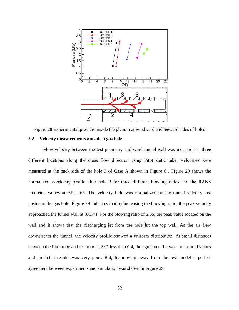
52
Figure 28 Experimental pressure inside the plenum at windward and leeward sides of holes
5.2 Velocity measurements outside a gas hole
Flow velocity between the test geometry and wind tunnel wall was measured at three
different locations along the cross flow direction using Pitot static tube. Velocities were
measured at the back side of the hole 3 of Case A shown in Figure 6 . Figure 29 shows the
normalized x-velocity profile after hole 3 for three different blowing ratios and the RANS
predicted values at BR=2.65. The velocity field was normalized by the tunnel velocity just
upstream the gas hole. Figure 29 indicates that by increasing the blowing ratio, the peak velocity
approached the tunnel wall at X/D=1. For the blowing ratio of 2.65, the peak value located on the
wall and it shows that the discharging jet from the hole hit the top wall. As the air flew
downstream the tunnel, the velocity profile showed a uniform distribution. At small distances
between the Pitot tube and test model, S/D less than 0.4, the agreement between measured values
and predicted results was very poor. But, by moving away from the test model a perfect
agreement between experiments and simulation was shown in Figure 29.
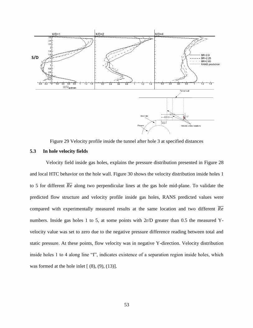
53
Figure 29 Velocity profile inside the tunnel after hole 3 at specified distances
5.3 In hole velocity fields
Velocity field inside gas holes, explains the pressure distribution presented in Figure 28
and local HTC behavior on the hole wall. Figure 30 shows the velocity distribution inside holes 1
to 5 for different 𝑅𝑒 along two perpendicular lines at the gas hole mid-plane. To validate the
predicted flow structure and velocity profile inside gas holes, RANS predicted values were
compared with experimentally measured results at the same location and two different 𝑅𝑒
numbers. Inside gas holes 1 to 5, at some points with 2r/D greater than 0.5 the measured Y-
velocity value was set to zero due to the negative pressure difference reading between total and
static pressure. At these points, flow velocity was in negative Y-direction. Velocity distribution
inside holes 1 to 4 along line “I”, indicates existence of a separation region inside holes, which
was formed at the hole inlet [ (8), (9), (13)].
S/D
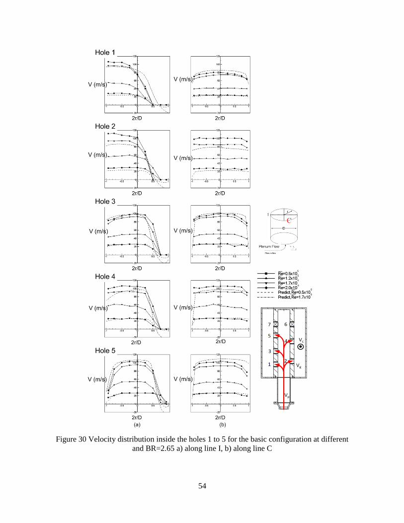
54
Figure 30 Velocity distribution inside the holes 1 to 5 for the basic configuration at different
and BR=2.65 a) along line I, b) along line C
55
The recirculation region size was depended on Reynolds number and a slight decrease
from hole 1 to 5 was seen. The decreasing trend on recirculation bubble size was due to the
decreasing trend of plenum flow velocity from hole 1 to 5. In Figure 30, the velocity profile
inside the 5th
hole had a symmetrical shape which was an answer to pressure values shown in
Figure 28. Numerical prediction was validated with experimentally measured velocity values due
to the great agreement presented in Figure 30.
Figure 31 shows predicted Y-velocity contour maps and stream traces inside each hole.
Zero velocity regions inside gas holes indicated the separation zone. In hole 1 to 4, the separation
region was big and discharged into the tunnel flow.
In holes 1 and 2, the difference in separation region size was very small due to small
change in plenum velocity from hole 1 to 2. Stream traces indicated that for these two holes,
plenum flow was divided at the hole inlet. So, the entering flow into the hole 1 and 2 strongly
impinges the aft-side of the hole and was separated on the fore-side of the hole. In hole 3,
plenum flow was divided inside the feed tube at a short distance after the hole inlet. So, a weak
flow leaked into the hole from the aft-side. This indicates that flow impingement on the wall was
not as strong as what happens in first two gas holes. In hole 4, a weak flow turns into the hole
from the aft-side and generates a very small separation bubble on this side of the hole. This small
separation region altered the velocity profile and pushed the peak of the velocity profile to the
hole center. In this hole, plenum flow was not impinging the aft-side of the hole.
In 5th
hole, the flow field was an extreme situation of the 4th
hole flow distribution. The
flow turning into the hole from the aft-side of the hole was strong enough to form a separation
bubble on that side of the hole. Because of the recirculation bubble, maximum velocity value
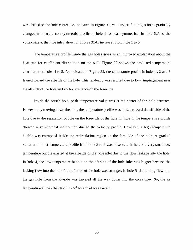
56
was shifted to the hole center. As indicated in Figure 31, velocity profile in gas holes gradually
changed from truly non-symmetric profile in hole 1 to near symmetrical in hole 5;Also the
vortex size at the hole inlet, shown in Figure 31-b, increased from hole 1 to 5.
The temperature profile inside the gas holes gives us an improved explanation about the
heat transfer coefficient distribution on the wall. Figure 32 shows the predicted temperature
distribution in holes 1 to 5. As indicated in Figure 32, the temperature profile in holes 1, 2 and 3
leaned toward the aft-side of the hole. This tendency was resulted due to flow impingement near
the aft side of the hole and vortex existence on the fore-side.
Inside the fourth hole, peak temperature value was at the center of the hole entrance.
However, by moving down the hole, the temperature profile was biased toward the aft-side of the
hole due to the separation bubble on the fore-side of the hole. In hole 5, the temperature profile
showed a symmetrical distribution due to the velocity profile. However, a high temperature
bubble was entrapped inside the recirculation region on the fore-side of the hole. A gradual
variation in inlet temperature profile from hole 3 to 5 was observed. In hole 3 a very small low
temperature bubble existed at the aft-side of the hole inlet due to the flow leakage into the hole.
In hole 4, the low temperature bubble on the aft-side of the hole inlet was bigger because the
leaking flow into the hole from aft-side of the hole was stronger. In hole 5, the turning flow into
the gas hole from the aft-side was traveled all the way down into the cross flow. So, the air
temperature at the aft-side of the 5th
hole inlet was lowest.
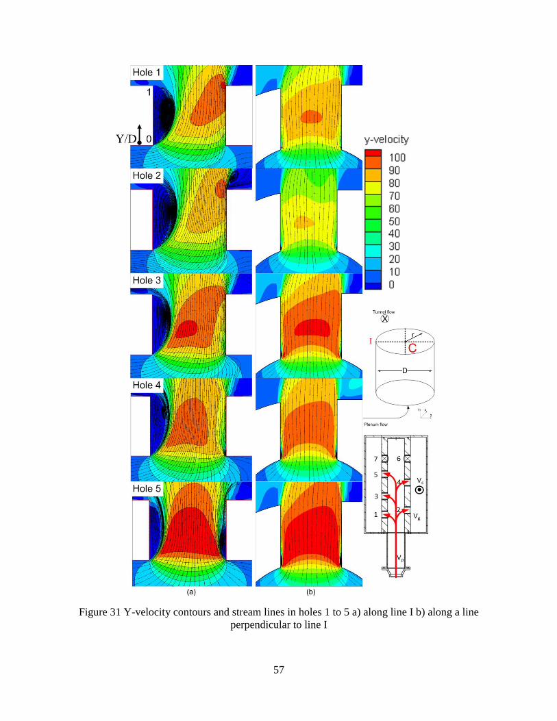
57
Figure 31 Y-velocity contours and stream lines in holes 1 to 5 a) along line I b) along a line
perpendicular to line I
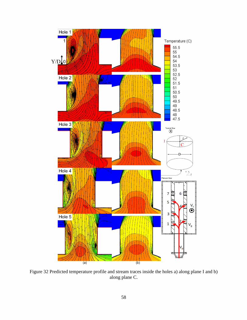
58
Figure 32 Predicted temperature profile and stream traces inside the holes a) along plane I and b)
along plane C.

59
5.4 Heat transfer
Heat transfer coefficient was measured by a transient test and semi infinite body heat
conduction assumption using IR-thermography. Figure 33 shows normalized Nusselt number
contour map inside holes 1 to 5 for different 𝑅𝑒 . Nusselt number values were normalized by
fully developed turbulent pipe flow Nusselt number (1) for corresponding Reynolds number.
Circumferential non-uniformity in HTC distribution inside gas holes was seen in Figure
33 due to non-uniform velocity profile. As indicated, for all holes high HTC value region was
more spread out for 𝑅𝑒 =0.5×10⁵ than 𝑅𝑒 =2.0×10
5. By increasing the Reynolds number, the
recirculation region size increases and expands low HTC region inside the holes.
For holes 1 to 4, heat transfer peak value existed at -45o<θ<+45
o and 0<Y/D<0.25. For
the hole 1 and 2 as explained by velocity contour maps, plenum flow hit the aft-side of the hole
inlet and got divided. So, flow impingement at the inlet of the hole caused a high heat transfer
region. In hole 3 despite the plenum flow was divided at a short distance after the hole inlet, a
high HTC region stands inside the hole near its inlet. Inside the 4th
hole, flow pattern was
different and due to small vortex on the aft-side of the hole inlet, high HTC value exists a short
distance down the hole. Also, high HTC magnitude in hole 4 was lower than that of holes 1 to 3.
In hole 5, velocity profile was near symmetrical and local HTC distribution was
approximately uniform. In this hole, a significant separation region existed on the aft-side of the
hole and the hole wall was not impinged by the flow. Due to the existence of recirculation bubble
at both sides of a the fifth gas hole, velocity profile and local HTC distribution had a more
uniform pattern.

60
Figure 33 Normalized Nusselt number in hole contour maps for basic configuration, BR=2.65 a)
Re=0.5x10⁵, b) Re=1.2x10
5, c) Re=1.7x10
5, d) Re=2.0x10
5
The circumferential non-uniform distribution of heat transfer coefficient at the inlet of
gas holes 1 to 5 (Y/D=0.05) was presented in Figure 34 and Figure 35. As shown, at gas hole 1,
61
flow impingement effect was strongest and brings a value of 9 for normalized Nusselt number.
However, the impingement heat transfer coefficient in holes 2 to 5 was much less. Also, the
decrease in impingement heat transfer coefficient from gas hole 1 to 2 was far greater than
decrease of that from hole 2 to 4. In gas hole 5, the trend of circumferential variation of HTC
was flat and flow impingement inside the gas hole was not observed which was in agreement
with velocity profile and pressure measurement results. In Figure 35, a perfect agreement with
measured values and predicted HTC results at the inlet of gas holes is observed. The perfection
of agreement between numerical and experimental values validates the accuracy of turbulence
method and near wall treatment scheme chosen for this project.
Figure 34 Circumferential variation of HTC at the inlet of gas holes 1 to 5 at Y/D=0.05 for basic
configuration (Re=1.7x10⁵ and BR=2.65)
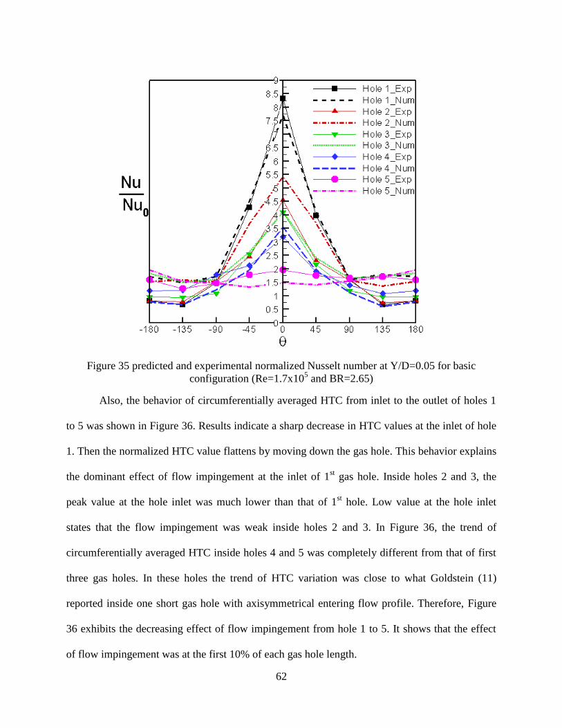
62
Figure 35 predicted and experimental normalized Nusselt number at Y/D=0.05 for basic
configuration (Re=1.7x10⁵ and BR=2.65)
Also, the behavior of circumferentially averaged HTC from inlet to the outlet of holes 1
to 5 was shown in Figure 36. Results indicate a sharp decrease in HTC values at the inlet of hole
1. Then the normalized HTC value flattens by moving down the gas hole. This behavior explains
the dominant effect of flow impingement at the inlet of 1st gas hole. Inside holes 2 and 3, the
peak value at the hole inlet was much lower than that of 1st hole. Low value at the hole inlet
states that the flow impingement was weak inside holes 2 and 3. In Figure 36, the trend of
circumferentially averaged HTC inside holes 4 and 5 was completely different from that of first
three gas holes. In these holes the trend of HTC variation was close to what Goldstein (11)
reported inside one short gas hole with axisymmetrical entering flow profile. Therefore, Figure
36 exhibits the decreasing effect of flow impingement from hole 1 to 5. It shows that the effect
of flow impingement was at the first 10% of each gas hole length.
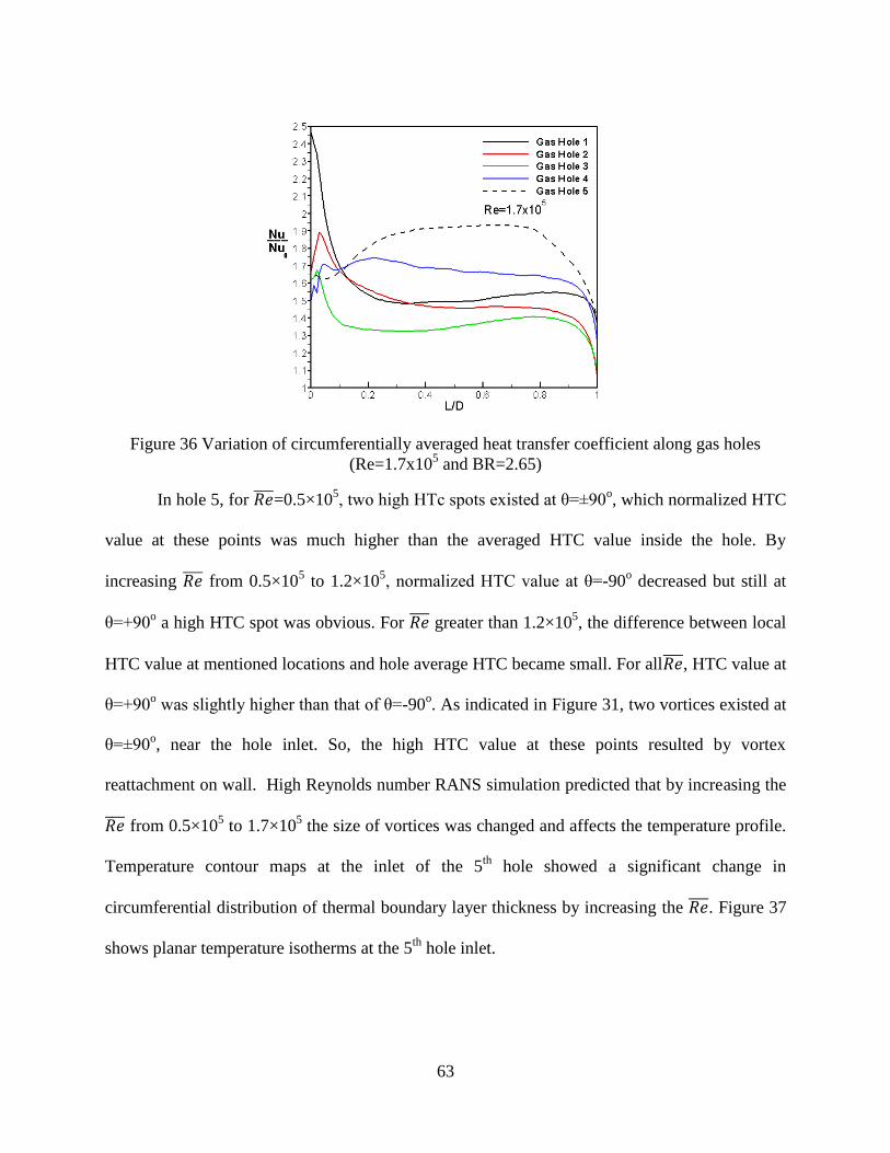
63
Figure 36 Variation of circumferentially averaged heat transfer coefficient along gas holes
(Re=1.7x10⁵ and BR=2.65)
In hole 5, for 𝑅𝑒 =0.5×10⁵, two high HTc spots existed at θ=±90
o, which normalized HTC
value at these points was much higher than the averaged HTC value inside the hole. By
increasing 𝑅𝑒 from 0.5×10⁵ to 1.2×10
5, normalized HTC value at θ=-90
o decreased but still at
θ=+90o a high HTC spot was obvious. For 𝑅𝑒 greater than 1.2×10
5, the difference between local
HTC value at mentioned locations and hole average HTC became small. For all𝑅𝑒 , HTC value at
θ=+90o was slightly higher than that of θ=-90
o. As indicated in Figure 31, two vortices existed at
θ=±90o, near the hole inlet. So, the high HTC value at these points resulted by vortex
reattachment on wall. High Reynolds number RANS simulation predicted that by increasing the
𝑅𝑒 from 0.5×10⁵ to 1.7×10
5 the size of vortices was changed and affects the temperature profile.
Temperature contour maps at the inlet of the 5th
hole showed a significant change in
circumferential distribution of thermal boundary layer thickness by increasing the 𝑅𝑒 . Figure 37
shows planar temperature isotherms at the 5th
hole inlet.
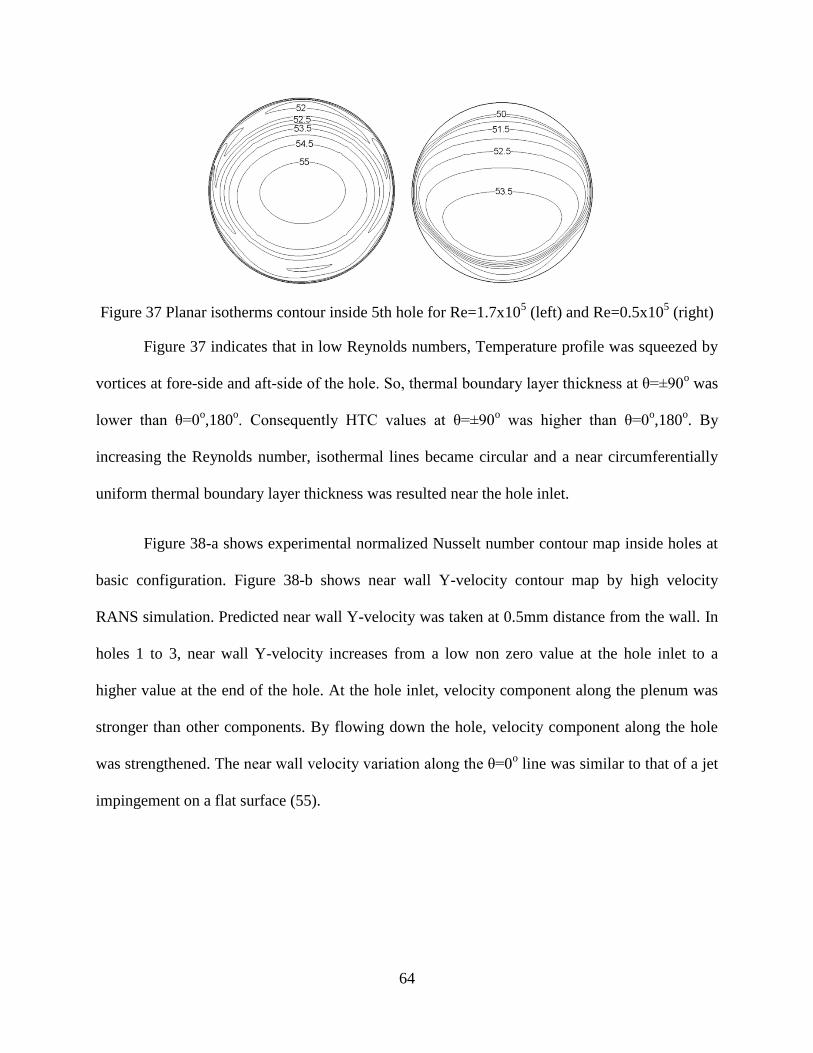
64
Figure 37 Planar isotherms contour inside 5th hole for Re=1.7x10⁵ (left) and Re=0.5x10
5 (right)
Figure 37 indicates that in low Reynolds numbers, Temperature profile was squeezed by
vortices at fore-side and aft-side of the hole. So, thermal boundary layer thickness at θ=±90o was
lower than θ=0o,180
o. Consequently HTC values at θ=±90
o was higher than θ=0
o,180
o. By
increasing the Reynolds number, isothermal lines became circular and a near circumferentially
uniform thermal boundary layer thickness was resulted near the hole inlet.
Figure 38-a shows experimental normalized Nusselt number contour map inside holes at
basic configuration. Figure 38-b shows near wall Y-velocity contour map by high velocity
RANS simulation. Predicted near wall Y-velocity was taken at 0.5mm distance from the wall. In
holes 1 to 3, near wall Y-velocity increases from a low non zero value at the hole inlet to a
higher value at the end of the hole. At the hole inlet, velocity component along the plenum was
stronger than other components. By flowing down the hole, velocity component along the hole
was strengthened. The near wall velocity variation along the θ=0o line was similar to that of a jet
impingement on a flat surface (55).
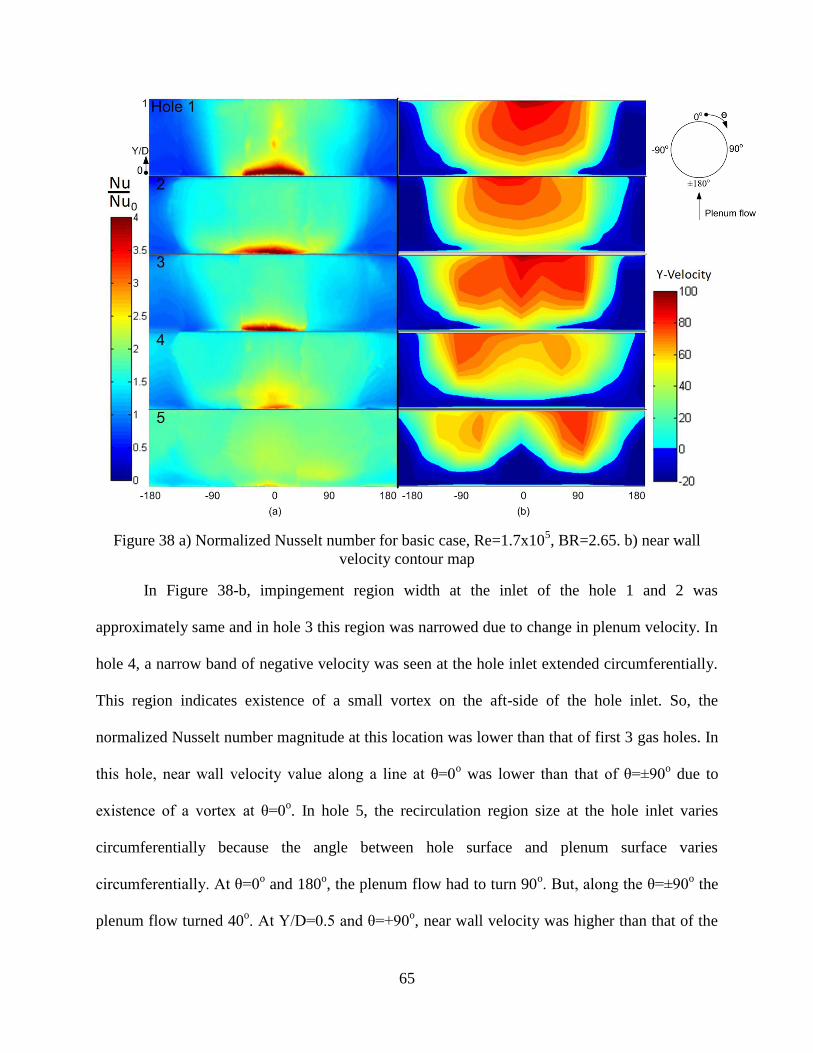
65
Figure 38 a) Normalized Nusselt number for basic case, Re=1.7x10⁵, BR=2.65. b) near wall
velocity contour map
In Figure 38-b, impingement region width at the inlet of the hole 1 and 2 was
approximately same and in hole 3 this region was narrowed due to change in plenum velocity. In
hole 4, a narrow band of negative velocity was seen at the hole inlet extended circumferentially.
This region indicates existence of a small vortex on the aft-side of the hole inlet. So, the
normalized Nusselt number magnitude at this location was lower than that of first 3 gas holes. In
this hole, near wall velocity value along a line at θ=0o was lower than that of θ=±90
o due to
existence of a vortex at θ=0o. In hole 5, the recirculation region size at the hole inlet varies
circumferentially because the angle between hole surface and plenum surface varies
circumferentially. At θ=0o and 180
o, the plenum flow had to turn 90
o. But, along the θ=±90
o the
plenum flow turned 40o. At Y/D=0.5 and θ=+90
o, near wall velocity was higher than that of the
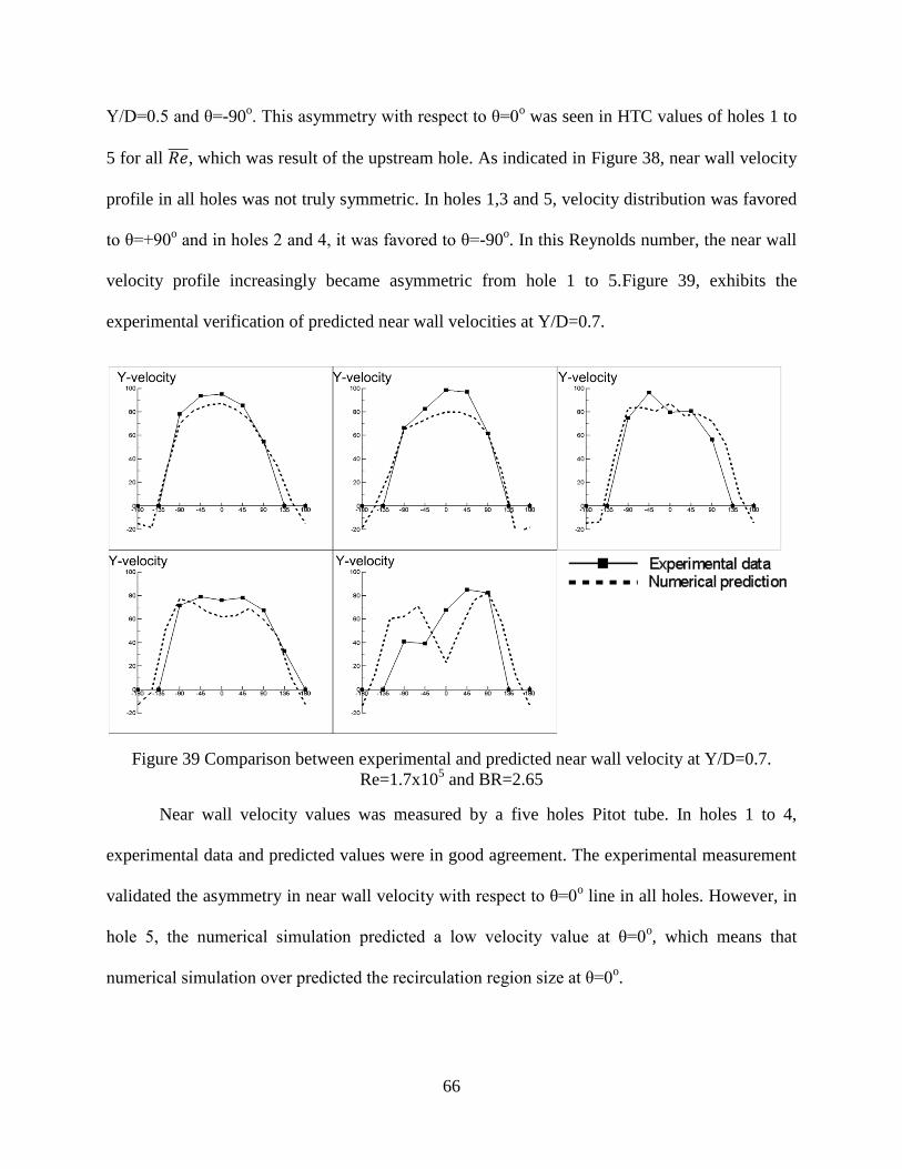
66
Y/D=0.5 and θ=-90o. This asymmetry with respect to θ=0
o was seen in HTC values of holes 1 to
5 for all 𝑅𝑒 , which was result of the upstream hole. As indicated in Figure 38, near wall velocity
profile in all holes was not truly symmetric. In holes 1,3 and 5, velocity distribution was favored
to θ=+90o and in holes 2 and 4, it was favored to θ=-90
o. In this Reynolds number, the near wall
velocity profile increasingly became asymmetric from hole 1 to 5.Figure 39, exhibits the
experimental verification of predicted near wall velocities at Y/D=0.7.
Figure 39 Comparison between experimental and predicted near wall velocity at Y/D=0.7.
Re=1.7x10⁵ and BR=2.65
Near wall velocity values was measured by a five holes Pitot tube. In holes 1 to 4,
experimental data and predicted values were in good agreement. The experimental measurement
validated the asymmetry in near wall velocity with respect to θ=0o line in all holes. However, in
hole 5, the numerical simulation predicted a low velocity value at θ=0o, which means that
numerical simulation over predicted the recirculation region size at θ=0o.
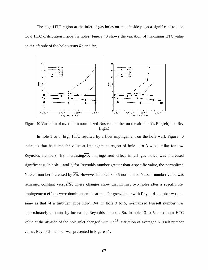
67
The high HTC region at the inlet of gas holes on the aft-side plays a significant role on
local HTC distribution inside the holes. Figure 40 shows the variation of maximum HTC value
on the aft-side of the hole versus 𝑅𝑒 and ReL.
Figure 40 Variation of maximum normalized Nusselt number on the aft-side Vs Re (left) and ReL
(right)
In hole 1 to 3, high HTC resulted by a flow impingement on the hole wall. Figure 40
indicates that heat transfer value at impingement region of hole 1 to 3 was similar for low
Reynolds numbers. By increasing𝑅𝑒 , impingement effect in all gas holes was increased
significantly. In hole 1 and 2, for Reynolds number greater than a specific value, the normalized
Nusselt number increased by 𝑅𝑒 . However in holes 3 to 5 normalized Nusselt number value was
remained constant versus𝑅𝑒 . These changes show that in first two holes after a specific Re,
impingement effects were dominant and heat transfer growth rate with Reynolds number was not
same as that of a turbulent pipe flow. But, in hole 3 to 5, normalized Nusselt number was
approximately constant by increasing Reynolds number. So, in holes 3 to 5, maximum HTC
value at the aft-side of the hole inlet changed with Re0.8
. Variation of averaged Nusselt number
versus Reynolds number was presented in Figure 41.
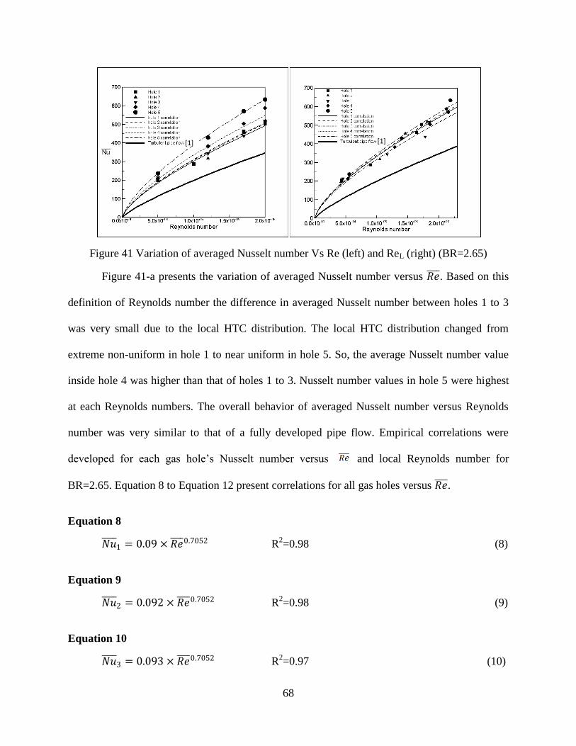
68
Figure 41 Variation of averaged Nusselt number Vs Re (left) and ReL (right) (BR=2.65)
Figure 41-a presents the variation of averaged Nusselt number versus 𝑅𝑒 . Based on this
definition of Reynolds number the difference in averaged Nusselt number between holes 1 to 3
was very small due to the local HTC distribution. The local HTC distribution changed from
extreme non-uniform in hole 1 to near uniform in hole 5. So, the average Nusselt number value
inside hole 4 was higher than that of holes 1 to 3. Nusselt number values in hole 5 were highest
at each Reynolds numbers. The overall behavior of averaged Nusselt number versus Reynolds
number was very similar to that of a fully developed pipe flow. Empirical correlations were
developed for each gas hole’s Nusselt number versus and local Reynolds number for
BR=2.65. Equation 8 to Equation 12 present correlations for all gas holes versus 𝑅𝑒 .
Equation 8
𝑁𝑢 1 = 0.09 × 𝑅𝑒 0.7052 R2=0.98 (8)
Equation 9
𝑁𝑢 2 = 0.092 × 𝑅𝑒 0.7052 R2=0.98 (9)
Equation 10
𝑁𝑢 3 = 0.093 × 𝑅𝑒 0.7052 R2=0.97 (10)
[1] [1]

69
Equation 11
𝑁𝑢 4 = 0.1 × 𝑅𝑒 0.7052 R2=0.98 (11)
Equation 12
𝑁𝑢 5 = 0.116 × 𝑅𝑒 0.7052 R2=0.98 (12)
Figure 41 also presents the variation of averaged Nusselt number versus ReL. For one
specific 𝑅𝑒 , ReL was increased from hole 1 to 5 due to the reduction in recirculation region size
in holes 1 to 5. As shown in Figure 41 all data were in a narrow band for results versus ReL and
empirical correlation was developed for all gas holes. Equation 13 presents a correlation for all
gas holes versus ReL.
Equation 13
𝑁𝑢 2 = 0.1 × 𝑅𝑒𝐿0.7052
R2=0.97
In hole 5, because of the near-symmetrical velocity profile inside the hole, averaged
Nusselt numbers inside were combined with that of a short hole (8). Figure 42 exhibits the
agreement between averaged Nusselt number in hole 5 and inside a short hole with
axisymmetrical flow. Cho et al (8) correlation was compared with hole 5 correlation and a new
correlation was developed for all data covering both Cho et al (8) and current study Reynolds
number ranges.
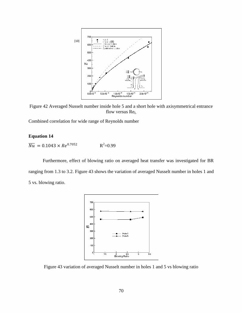
70
Figure 42 Averaged Nusselt number inside hole 5 and a short hole with axisymmetrical entrance
flow versus ReL
Combined correlation for wide range of Reynolds number
Equation 14
𝑁𝑢 = 0.1043 × 𝑅𝑒0.7052 R2=0.99
Furthermore, effect of blowing ratio on averaged heat transfer was investigated for BR
ranging from 1.3 to 3.2. Figure 43 shows the variation of averaged Nusselt number in holes 1 and
5 vs. blowing ratio.
Figure 43 variation of averaged Nusselt number in holes 1 and 5 vs blowing ratio
[10] (8)
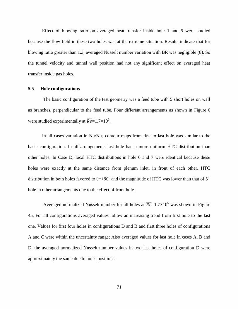
71
Effect of blowing ratio on averaged heat transfer inside hole 1 and 5 were studied
because the flow field in these two holes was at the extreme situation. Results indicate that for
blowing ratio greater than 1.3, averaged Nusselt number variation with BR was negligible (8). So
the tunnel velocity and tunnel wall position had not any significant effect on averaged heat
transfer inside gas holes.
5.5 Hole configurations
The basic configuration of the test geometry was a feed tube with 5 short holes on wall
as branches, perpendicular to the feed tube. Four different arrangements as shown in Figure 6
were studied experimentally at 𝑅𝑒 =1.7×10⁵.
In all cases variation in Nu/Nu0 contour maps from first to last hole was similar to the
basic configuration. In all arrangements last hole had a more uniform HTC distribution than
other holes. In Case D, local HTC distributions in hole 6 and 7 were identical because these
holes were exactly at the same distance from plenum inlet, in front of each other. HTC
distribution in both holes favored to θ=+90o and the magnitude of HTC was lower than that of 5
th
hole in other arrangements due to the effect of front hole.
Averaged normalized Nusselt number for all holes at 𝑅𝑒 =1.7×10⁵ was shown in Figure
45. For all configurations averaged values follow an increasing trend from first hole to the last
one. Values for first four holes in configurations D and B and first three holes of configurations
A and C were within the uncertainty range; Also averaged values for last hole in cases A, B and
D. the averaged normalized Nusselt number values in two last holes of configuration D were
approximately the same due to holes positions.
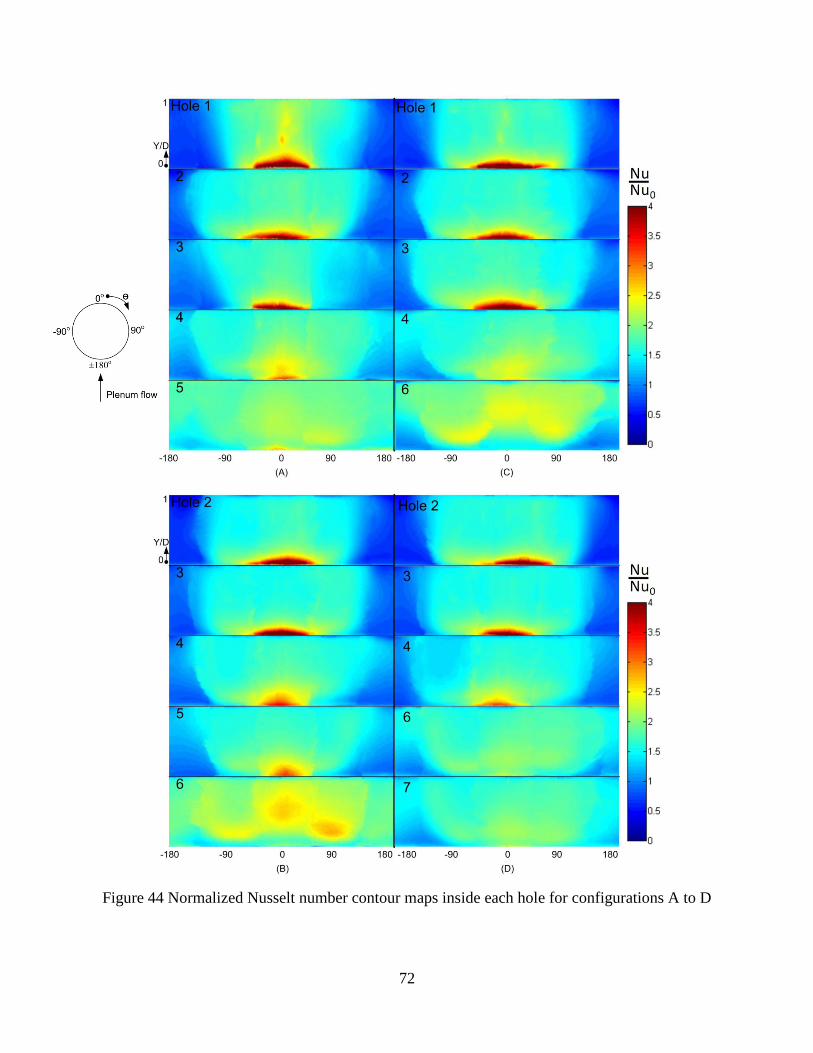
72
Figure 44 Normalized Nusselt number contour maps inside each hole for configurations A to D
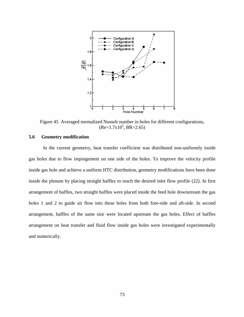
73
Figure 45 Averaged normalized Nusselt number in holes for different configurations,
(Re=1.7x10⁵, BR=2.65)
5.6 Geometry modification
In the current geometry, heat transfer coefficient was distributed non-uniformly inside
gas holes due to flow impingement on one side of the holes. To improve the velocity profile
inside gas hole and achieve a uniform HTC distribution, geometry modifications have been done
inside the plenum by placing straight baffles to reach the desired inlet flow profile (22). In first
arrangement of baffles, two straight baffles were placed inside the feed hole downstream the gas
holes 1 and 2 to guide air flow into these holes from both fore-side and aft-side. In second
arrangement, baffles of the same size were located upstream the gas holes. Effect of baffles
arrangement on heat transfer and fluid flow inside gas holes were investigated experimentally
and numerically.
74
5.6.1 Baffles placed downstream holes 1 and 2
5.6.1.1 Geometrical considerations
The geometry of the test section with baffles placed inside the feed hole was shown in
Figure 7. The baffle height was half of the gas hole diameter and placed half of the gas hole
diameter downstream gas holes 1 and 2. Baffle size was chosen among three different sizes in
order to distribute mass flow rate uniformly among gas holes.
Existence of baffles at the back of the gas holes returns a portion of flow against the
direction of main feed hole flow. So, small portion of the hole mass flow rate enters the hole
from aft-side of the hole and decreases the impingement effect inside the gas hole similar to what
happens inside holes 4 and 5. Figure 46 shows a schematic of how flow turns into gas holes with
and without baffles inside the feed hole. It exhibits that how baffles return a portion of plenum
flow into the gas holes 1 and 2.
5.6.1.2 Velocity measurement
The flow velocity along gas hole was measured at the mid-plane of each hole using Pitot static
tube. Figure 47 shows the axial velocity comparison at the gas hole mid-plane for first baffled
and non-baffled cases. In Figure 47, velocity profile inside holes 1 and 2 was qualitatively
similar for both baffled and non-baffled geometries. However, the recirculation region for
baffled geometry was half of the size of that of non-baffled geometry. Also, the maximum
velocity at 2r/D=-1 for baffled geometry was lower than that of non-baffled geometry. These
differences in velocity profiles were caused by the portion of the plenum flow returned into the
gas hole inlet by baffles. This flow enters gas hole from aft-side and generates a small
recirculation at that side.
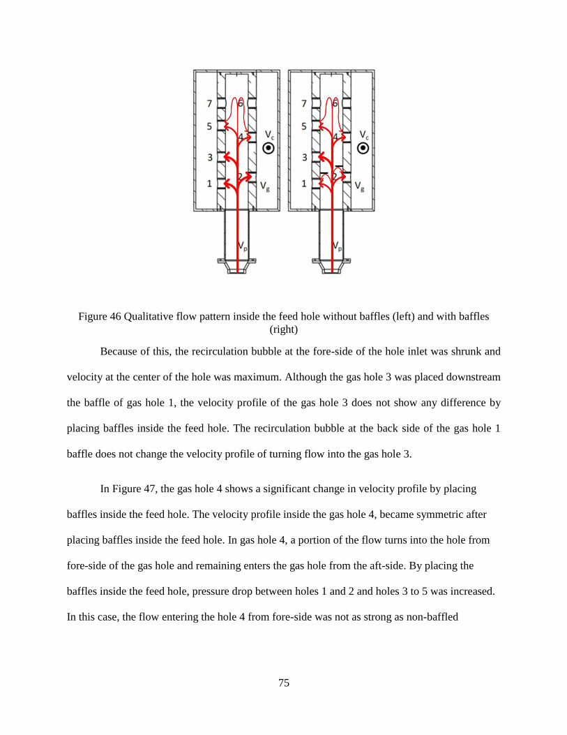
75
Figure 46 Qualitative flow pattern inside the feed hole without baffles (left) and with baffles
(right)
Because of this, the recirculation bubble at the fore-side of the hole inlet was shrunk and
velocity at the center of the hole was maximum. Although the gas hole 3 was placed downstream
the baffle of gas hole 1, the velocity profile of the gas hole 3 does not show any difference by
placing baffles inside the feed hole. The recirculation bubble at the back side of the gas hole 1
baffle does not change the velocity profile of turning flow into the gas hole 3.
In Figure 47, the gas hole 4 shows a significant change in velocity profile by placing
baffles inside the feed hole. The velocity profile inside the gas hole 4, became symmetric after
placing baffles inside the feed hole. In gas hole 4, a portion of the flow turns into the hole from
fore-side of the gas hole and remaining enters the gas hole from the aft-side. By placing the
baffles inside the feed hole, pressure drop between holes 1 and 2 and holes 3 to 5 was increased.
In this case, the flow entering the hole 4 from fore-side was not as strong as non-baffled
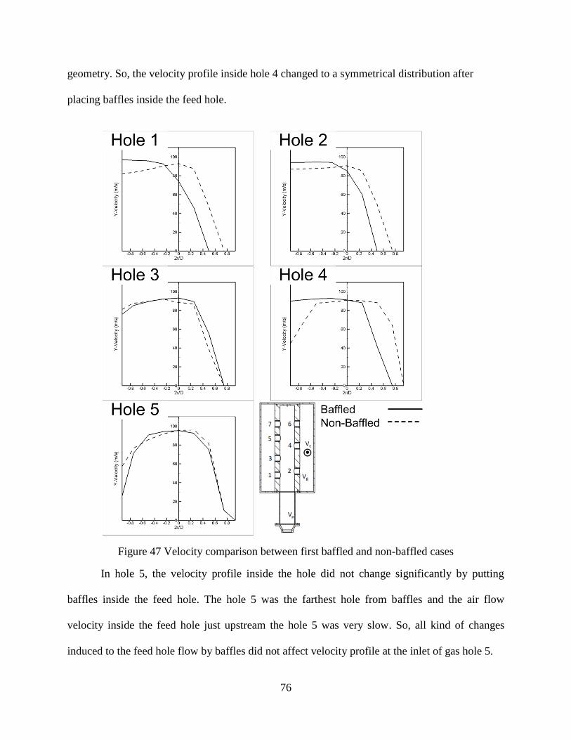
76
geometry. So, the velocity profile inside hole 4 changed to a symmetrical distribution after
placing baffles inside the feed hole.
Figure 47 Velocity comparison between first baffled and non-baffled cases
In hole 5, the velocity profile inside the hole did not change significantly by putting
baffles inside the feed hole. The hole 5 was the farthest hole from baffles and the air flow
velocity inside the feed hole just upstream the hole 5 was very slow. So, all kind of changes
induced to the feed hole flow by baffles did not affect velocity profile at the inlet of gas hole 5.

77
5.6.1.3 Heat transfer measurements
Similar to the heat transfer experiments for non-baffled geometry, heat transfer
measurement tests have been performed inside all gas holes for modified geometry. The
experimental 𝑅𝑒 was 1.7×10⁵
and blowing ratio kept 2.65. Figure 48 shows the normalized heat
transfer coefficient contour plots inside gas holes 1 to 5.
Figure 48 Normalized heat transfer coefficient contour plots inside gas holes 1 to 5 for baffled
(left) and non-baffled (right) geometries
As exhibited in Figure 48, the pattern of heat transfer coefficient inside gas holes was
same for both baffled and non-baffled geometries. However, for baffled geometry, the difference
between highest and lowest HTC values was smaller than that of non-baffled geometry. The
HTC value at -45o<θ<+45
o was decreased specially in hole 1 and was increased at +135
o<θ, θ<-
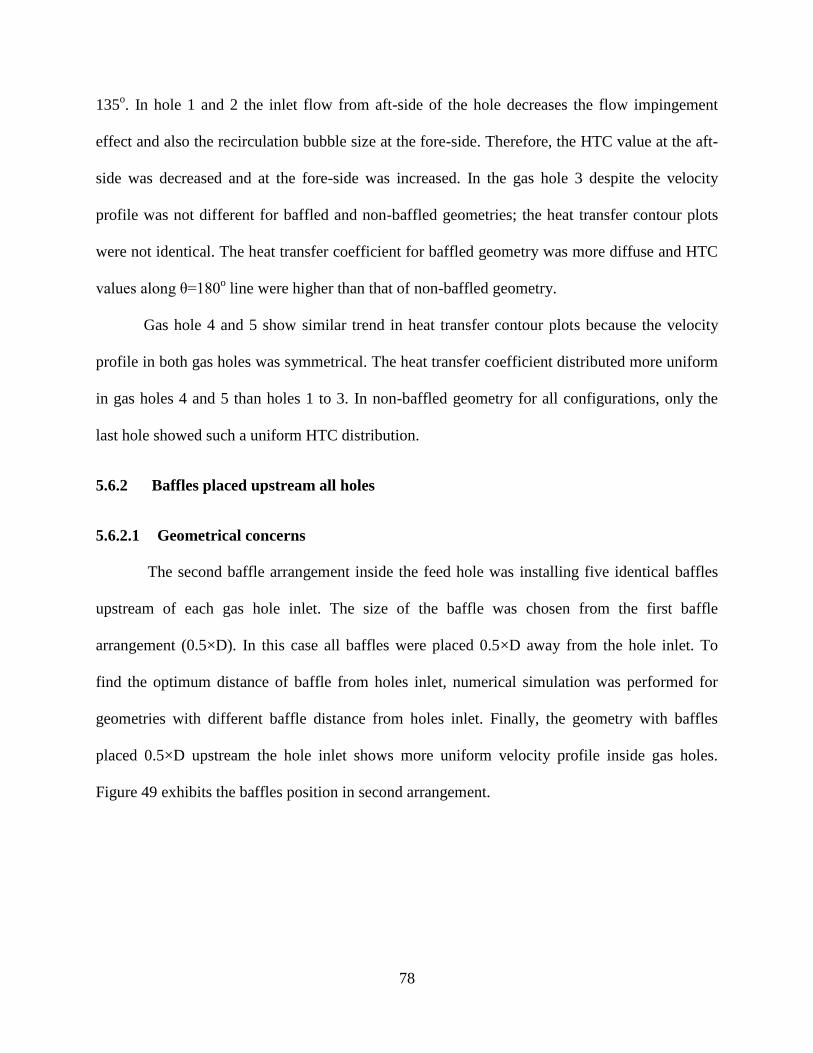
78
135o. In hole 1 and 2 the inlet flow from aft-side of the hole decreases the flow impingement
effect and also the recirculation bubble size at the fore-side. Therefore, the HTC value at the aft-
side was decreased and at the fore-side was increased. In the gas hole 3 despite the velocity
profile was not different for baffled and non-baffled geometries; the heat transfer contour plots
were not identical. The heat transfer coefficient for baffled geometry was more diffuse and HTC
values along θ=180o line were higher than that of non-baffled geometry.
Gas hole 4 and 5 show similar trend in heat transfer contour plots because the velocity
profile in both gas holes was symmetrical. The heat transfer coefficient distributed more uniform
in gas holes 4 and 5 than holes 1 to 3. In non-baffled geometry for all configurations, only the
last hole showed such a uniform HTC distribution.
5.6.2 Baffles placed upstream all holes
5.6.2.1 Geometrical concerns
The second baffle arrangement inside the feed hole was installing five identical baffles
upstream of each gas hole inlet. The size of the baffle was chosen from the first baffle
arrangement (0.5×D). In this case all baffles were placed 0.5×D away from the hole inlet. To
find the optimum distance of baffle from holes inlet, numerical simulation was performed for
geometries with different baffle distance from holes inlet. Finally, the geometry with baffles
placed 0.5×D upstream the hole inlet shows more uniform velocity profile inside gas holes.
Figure 49 exhibits the baffles position in second arrangement.
79
Figure 49 Schematic of fluid flow inside the feed hole without baffles (left) and second baffles
arrangement (right)
5.6.3 Velocity prediction
To investigate the effect of baffles placed upstream the holes inlet, velocity distribution
inside all holes was studied numerically. Figure 50 exhibits the velocity contour maps and stream
traces inside holes 1 to 5.
Results indicate a significant difference between non-baffled geometry and second
baffled arrangement. As presented in Figure 50, no recirculation region was observed at the fore-
side of holes 1 to 4. Inside holes 1 and 2, the velocity profile was approximately uniform. The
velocity magnitude was in a narrow range of 60 to 80. The high velocity region was detached
from the aft-side of the wall and a weak flow leaks into the hole from aft-side. Inside holes 3 to
5, velocity shows an axisymmetrical distribution. The peak velocity value stands at the center
line of holes. Stream traces enter gas holes 3 to 5 from both fore-side and aft-side. In hole 5, the
velocity profile did not change qualitatively. But, the recirculation bubble size at the aft-side of
the 5th
hole was increased after placing the baffle upstream of that hole. This enhancement in
recirculation bubble was due to decrease in strength of the flow entering gas hole from fore-side.

80
After placing baffle upstream the gas holes, the flow strength entering into the gas hole from aft-
side became dominant to flow strength entering gas hole from fore-side. Therefore, the
recirculation bubble size at the aft-side was increased by placing baffle upstream the 5th
hole
inlet.
Based on the previous experimental and numerical investigations, velocity distribution
profile has a significant effect on the heat transfer distribution inside gas holes. Non-uniform
velocity profile and flow impingement inside gas holes result a highly non-uniform heat transfer
distribution with high HTC magnitude at the hole inlet. Consequently, Figure 50 concludes a
uniform HTC distribution inside gas holes due to the velocity profile. Also, flow impingement
inside gas holes was not diagnosed when baffles were placed upstream the holes inlet.
5.6.4 Variable baffles height
Previous baffle arrangements prove the significant effect of baffles inside the feed hole
on gas holes flow structure. The velocity field inside gas holes can be manipulated by baffles
height and distance from holes inlet. The second baffle configuration shows that placing baffles
upstream gas holes, prevents formation of recirculation bubble and results better velocity profile
inside each hole. However, placing equi-height baffles upstream holes 1 to 5, resulted non-
uniform distribution of mass flow rate through holes 1 to 5. Therefore, to achieve the best baffle
configuration inside the plenum, two parameters were considered: minimizing the recirculation
bubble strength inside each hole and distributing the plenum mass flow rate into gas holes
evenly.

81
Figure 50 Velocity contour plots and stream traces inside all holes for a) non-baffled geometry,
b) Second baffled arrangement
5.6.4.1 Optimization parameters
The strategy of choosing the best baffle height and distance from gas holes inlet will be
discussed initially for one averaged Reynolds number. Geometrical parameters governing heat
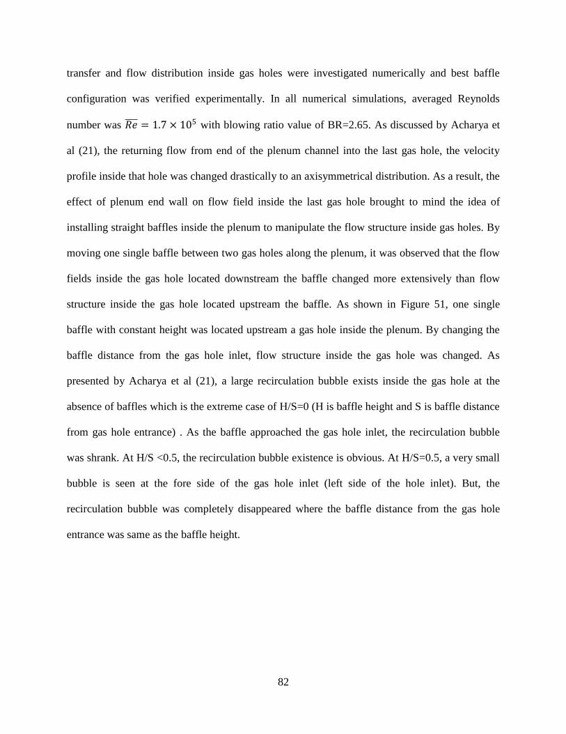
82
transfer and flow distribution inside gas holes were investigated numerically and best baffle
configuration was verified experimentally. In all numerical simulations, averaged Reynolds
number was 𝑅𝑒 = 1.7 × 10⁵ with blowing ratio value of BR=2.65. As discussed by Acharya et
al (21), the returning flow from end of the plenum channel into the last gas hole, the velocity
profile inside that hole was changed drastically to an axisymmetrical distribution. As a result, the
effect of plenum end wall on flow field inside the last gas hole brought to mind the idea of
installing straight baffles inside the plenum to manipulate the flow structure inside gas holes. By
moving one single baffle between two gas holes along the plenum, it was observed that the flow
fields inside the gas hole located downstream the baffle changed more extensively than flow
structure inside the gas hole located upstream the baffle. As shown in Figure 51, one single
baffle with constant height was located upstream a gas hole inside the plenum. By changing the
baffle distance from the gas hole inlet, flow structure inside the gas hole was changed. As
presented by Acharya et al (21), a large recirculation bubble exists inside the gas hole at the
absence of baffles which is the extreme case of H/S=0 (H is baffle height and S is baffle distance
from gas hole entrance) . As the baffle approached the gas hole inlet, the recirculation bubble
was shrank. At H/S <0.5, the recirculation bubble existence is obvious. At H/S=0.5, a very small
bubble is seen at the fore side of the gas hole inlet (left side of the hole inlet). But, the
recirculation bubble was completely disappeared where the baffle distance from the gas hole
entrance was same as the baffle height.

83
Figure 51 Effect of baffle distance on flow structure inside one gas hole ((Re) ̅=1.7×10⁵,
BR=2.65)
Moreover, to investigate the effect of H/S ratio over one, the baffle height was changed
while baffle distance was kept constant from the gas hole inlet. Figure 52 exhibits the baffle
height effect on flow field inside a gas hole located downstream the baffle. As presented, at H/S
ratio of one, no recirculation bubble exists inside the gas hole. However, by increasing the H/S
over one, a recirculation bubble forms at the aft side of the gas hole inlet, where previously
indicated as impingement region.
Figure 52 Flow structure inside a gas hole for H/S ratio greater than one (Re=1.7×10⁵, BR=2.65)
By investigating the effect of baffle height “H” and baffle distance from gas hole “S”, on
flow structure inside gas holes, it was found that the vortex formation inside gas hole
downstream a baffle can be characterized manipulated by “H/S” ratio. Based on the results
indicated in Figure 51 and Figure 52, recirculation bubble inside a gas hole located downstream a
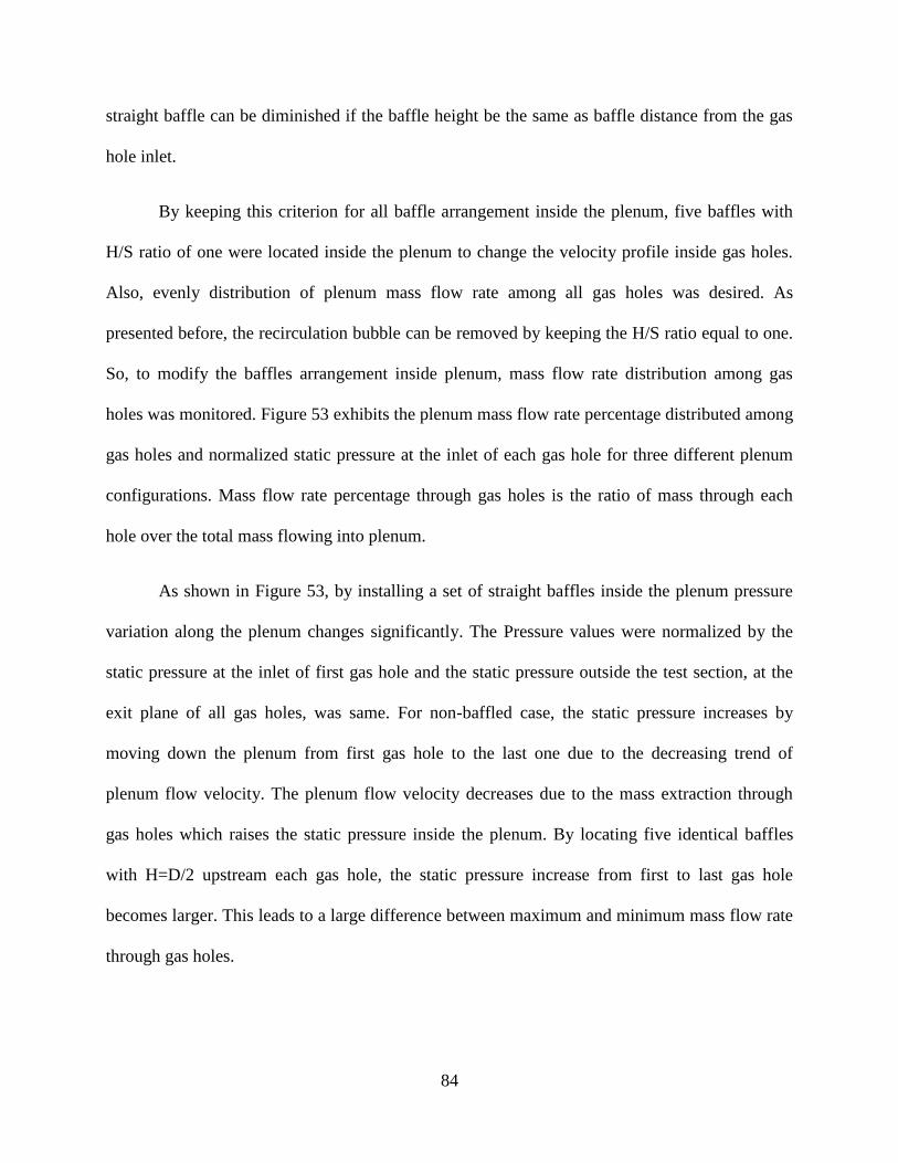
84
straight baffle can be diminished if the baffle height be the same as baffle distance from the gas
hole inlet.
By keeping this criterion for all baffle arrangement inside the plenum, five baffles with
H/S ratio of one were located inside the plenum to change the velocity profile inside gas holes.
Also, evenly distribution of plenum mass flow rate among all gas holes was desired. As
presented before, the recirculation bubble can be removed by keeping the H/S ratio equal to one.
So, to modify the baffles arrangement inside plenum, mass flow rate distribution among gas
holes was monitored. Figure 53 exhibits the plenum mass flow rate percentage distributed among
gas holes and normalized static pressure at the inlet of each gas hole for three different plenum
configurations. Mass flow rate percentage through gas holes is the ratio of mass through each
hole over the total mass flowing into plenum.
As shown in Figure 53, by installing a set of straight baffles inside the plenum pressure
variation along the plenum changes significantly. The Pressure values were normalized by the
static pressure at the inlet of first gas hole and the static pressure outside the test section, at the
exit plane of all gas holes, was same. For non-baffled case, the static pressure increases by
moving down the plenum from first gas hole to the last one due to the decreasing trend of
plenum flow velocity. The plenum flow velocity decreases due to the mass extraction through
gas holes which raises the static pressure inside the plenum. By locating five identical baffles
with H=D/2 upstream each gas hole, the static pressure increase from first to last gas hole
becomes larger. This leads to a large difference between maximum and minimum mass flow rate
through gas holes.
85
As presented in Figure 53, the static pressure at the inlet of first gas hole is much smaller
than static pressure at the inlet of last gas hole. This drastic change in static pressure for identical
baffle arrangement case was resulted by the high plenum velocity above first two baffles which
generates strong recirculation bubble at the back of those baffles. Because of the decreasing
trend of the plenum velocity along the plenum, the vortex strength at the back of straight baffles
was decreased from the first to the last gas hole.
Therefore, to manipulate the trend of static pressure at the inlet of gas holes, vortex
strength at the back of straight baffles was controlled by changing the baffle height. To reduce
the vortex strength at the inlet of first two gas holes, first two baffles were shortened but H/S
ratio was kept one. Several different cases with different combination of baffle heights were
simulated numerically to reach the best baffle configuration. In the best baffle arrangement case,
one short baffle was located downstream the last gas hole as well to prevent the vortex formation
at the aft side of the fifth hole due to the returning plenum flow shown in Figure 54. The H/S
ratio of this small baffle was kept one too. As indicated in Figure 53, for the best baffle
arrangement case, mass flow rate percentage through gas holes 2 and 3 was 2% off from the
ideal value of 20%, but for all other gas holes this value was ideal. In the modified configuration
of straight baffles inside the plenum the height of two baffles located upstream of holes 1 and 2
was D/4. Three baffles of height D were placed upstream of holes 3, 4 and 5 and the height of the
baffle downstream the last gas hole was D/4. Figure 54 exhibits the stream traces and velocity
contour maps inside cooling holes for non-baffled and modified baffled configuration.
86
Figure 53 Normalized static pressure trend inside plenum (solid symbols), mass flow rate
percentage of each gas hole (hollow symbols) ((Re) ̅=1.7×10⁵, BR=2.65)
Figure 54 compares the flow structure inside gas holes for non-baffled plenum and
modified baffle configuration inside the plenum. The major difference in flow structure between
these two configurations was recirculation bubble existence inside gas holes. As shown in Figure
54-a, recirculation bubble occupies a significant portion of each gas hole volume. As studied by
Acharya et al (21), the recirculation bubble plays a significant role in heat transfer coefficient
distribution inside gas holes and leads to a highly non-uniform distribution of HTC on gas holes
wall. As a result, uniform distribution of heat transfer coefficient inside gas holes was expected
for the modified baffle arrangement. Also, Figure 54 indicates that for the best baffle
configuration inside the plenum, the difference between highest and lowest local velocity inside
gas holes was reduced.
To validate the numerically predicted velocity field inside cooling holes, velocity profile
inside gas holes was measured experimentally using a hot wire anemometer. Figure 55 exhibits
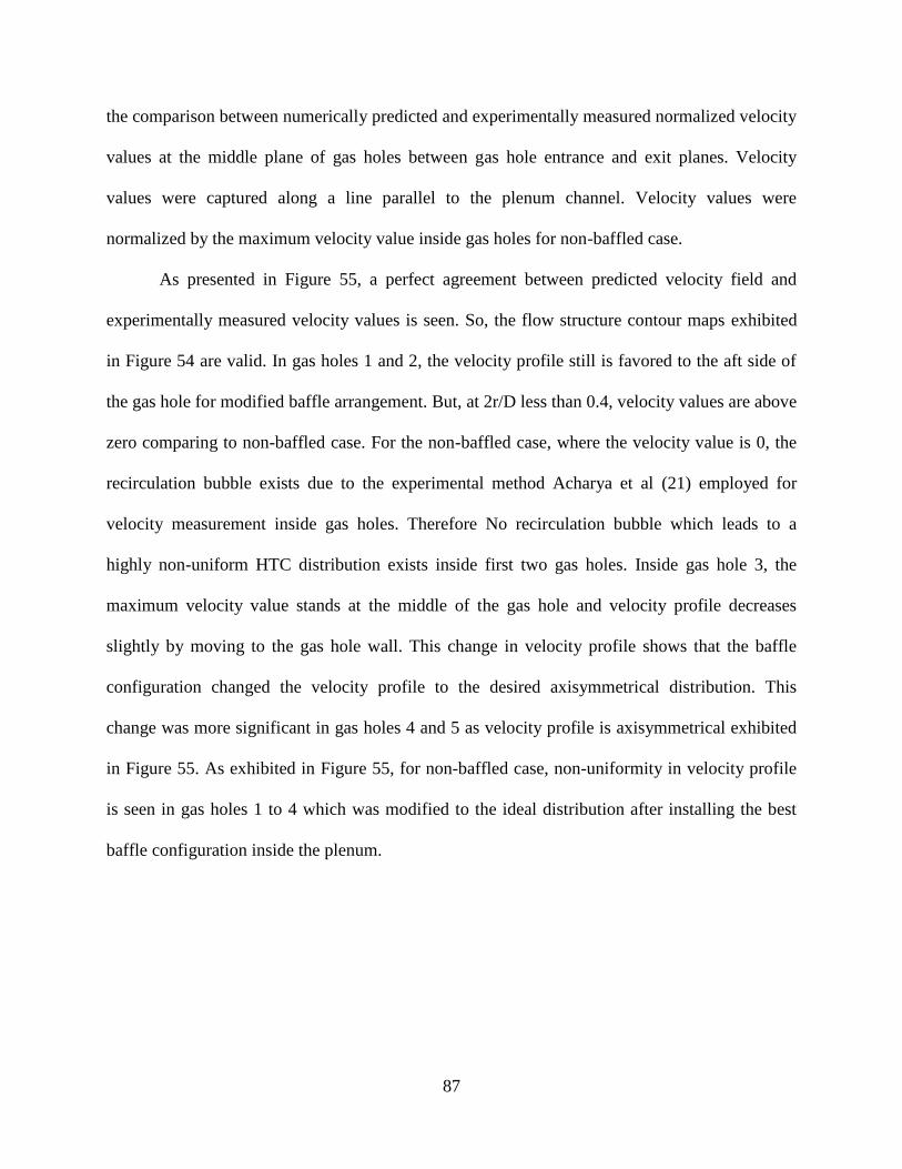
87
the comparison between numerically predicted and experimentally measured normalized velocity
values at the middle plane of gas holes between gas hole entrance and exit planes. Velocity
values were captured along a line parallel to the plenum channel. Velocity values were
normalized by the maximum velocity value inside gas holes for non-baffled case.
As presented in Figure 55, a perfect agreement between predicted velocity field and
experimentally measured velocity values is seen. So, the flow structure contour maps exhibited
in Figure 54 are valid. In gas holes 1 and 2, the velocity profile still is favored to the aft side of
the gas hole for modified baffle arrangement. But, at 2r/D less than 0.4, velocity values are above
zero comparing to non-baffled case. For the non-baffled case, where the velocity value is 0, the
recirculation bubble exists due to the experimental method Acharya et al (21) employed for
velocity measurement inside gas holes. Therefore No recirculation bubble which leads to a
highly non-uniform HTC distribution exists inside first two gas holes. Inside gas hole 3, the
maximum velocity value stands at the middle of the gas hole and velocity profile decreases
slightly by moving to the gas hole wall. This change in velocity profile shows that the baffle
configuration changed the velocity profile to the desired axisymmetrical distribution. This
change was more significant in gas holes 4 and 5 as velocity profile is axisymmetrical exhibited
in Figure 55. As exhibited in Figure 55, for non-baffled case, non-uniformity in velocity profile
is seen in gas holes 1 to 4 which was modified to the ideal distribution after installing the best
baffle configuration inside the plenum.
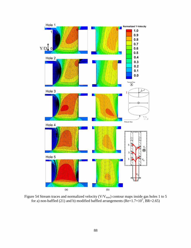
88
Figure 54 Stream traces and normalized velocity (V/Vmax) contour maps inside gas holes 1 to 5
for a) non-baffled (21) and b) modified baffled arrangements (Re=1.7×10⁵, BR=2.65)

89
Figure 55 Predicted and measured normalized velocity values for best baffle arrangement and
experimental velocity values for non-baffled (21). (Re=1.7×10⁵, BR=2.65)
Because of the flow structure presented in Figures 9 and 10, better distribution of the heat
transfer coefficient inside gas holes 1 to 5 is expected.
5.6.4.2 Baffle configuration heat transfer effect
Heat transfer coefficient inside gas holes was measured by employing IR thermography.
Figure 56 presents the local heat transfer coefficient contour maps inside all five gas holes for
both modified baffled and non-baffled configurations. As indicated in Figure 56, the heat transfer
coefficient distributed more uniform inside cooling holes for modified baffled geometry
comparing to non-baffled geometry. The difference between the highest and the lowest
normalized Nusselt number values decreased by installing modified arrangement of baffles
inside the plenum. The normalized Nusselt number values at θ=±180o were increased comparing
to non-baffled case especially in first three gas holes. This drastic change in heat transfer contour
plots at θ=±180o was resulted by the recirculation bubble elimination inside gas holes. Also, in
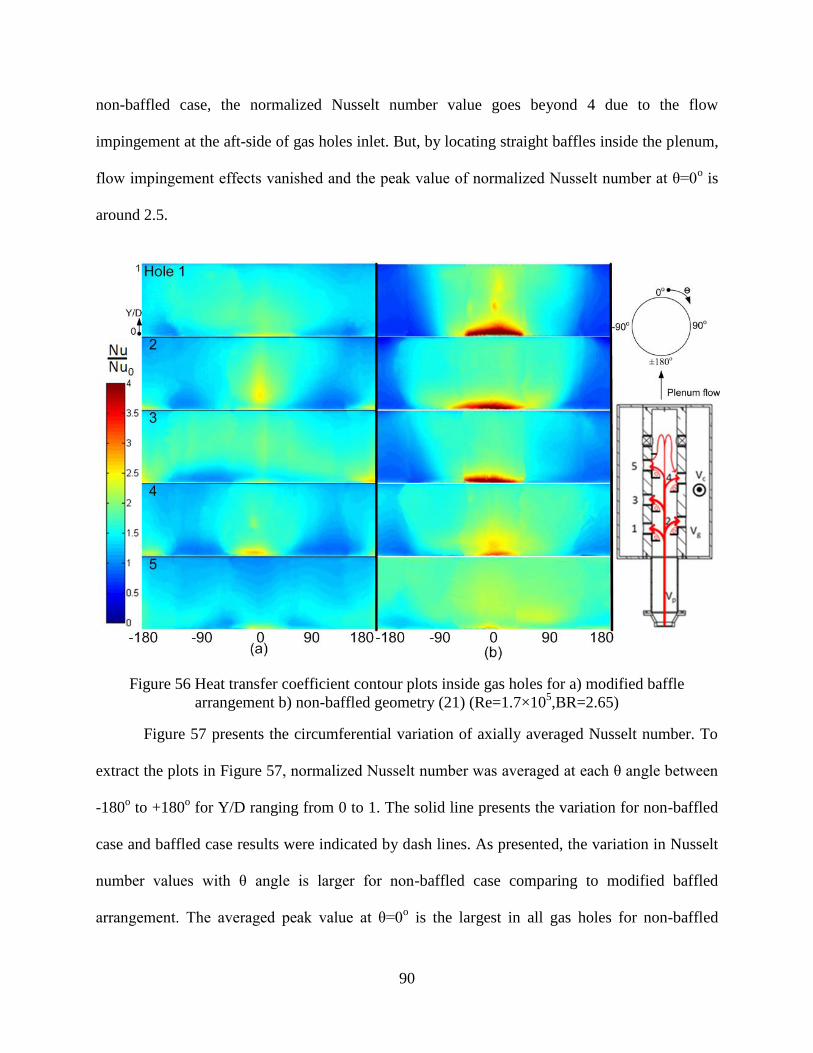
90
non-baffled case, the normalized Nusselt number value goes beyond 4 due to the flow
impingement at the aft-side of gas holes inlet. But, by locating straight baffles inside the plenum,
flow impingement effects vanished and the peak value of normalized Nusselt number at θ=0o is
around 2.5.
Figure 56 Heat transfer coefficient contour plots inside gas holes for a) modified baffle
arrangement b) non-baffled geometry (21) (Re=1.7×10⁵,BR=2.65)
Figure 57 presents the circumferential variation of axially averaged Nusselt number. To
extract the plots in Figure 57, normalized Nusselt number was averaged at each θ angle between
-180o to +180
o for Y/D ranging from 0 to 1. The solid line presents the variation for non-baffled
case and baffled case results were indicated by dash lines. As presented, the variation in Nusselt
number values with θ angle is larger for non-baffled case comparing to modified baffled
arrangement. The averaged peak value at θ=0o is the largest in all gas holes for non-baffled

91
situation and the smallest at θ=180o. However, for modified baffle arrangement case, normalized
Nusselt number variation with θ is very small in all gas holes which were expected from velocity
profile. Due to the short length of gas holes, the boundary layer on gas holes walls was very thin
and Nusselt number values are larger than Nusselt number values for fully developed pipe flow
regime. In Figure 58, Nusselt number was averaged circumferentially for θ ranging from -180o to
+180o at each Y/D. This figure validates the strong effect of flow impingement inside first three
gas holes for non-baffled case comparing to the baffled configuration. Due to the elimination of
recirculation region inside first three gas holes by placing baffles, circumferentially averaged
Nusselt number shows higher values at the mid-plane of the gas hole (Y/D=0.5) for baffled case
comparing to the non-baffled case in gas holes 1 and 2. In gas hole 3, the recirculation region
size is smaller comparing to gas holes 1 and 2 in non-baffled case. Therefore, the difference in
circumferentially averaged results between baffled and non-baffled cases is very small in gas
hole 3. However, circumferentially averaged Nusselt number trajectory for gas holes 4 and 5 in
baffled geometry is lower than that of non-baffled case due to the modification on mass flow rate
distribution among gas holes. In non-baffled case, more mass was flowing through gas holes 4
and 5 comparing to non-baffled case as shown in Figure 53. Figure 59 presents the averaged
Nusselt number values inside gas holes 1 to 5. As shown in Figure 59, averaged values for non-
baffled case were increased by moving down the plenum due to the drastic change in
recirculation bubble size inside gas holes.
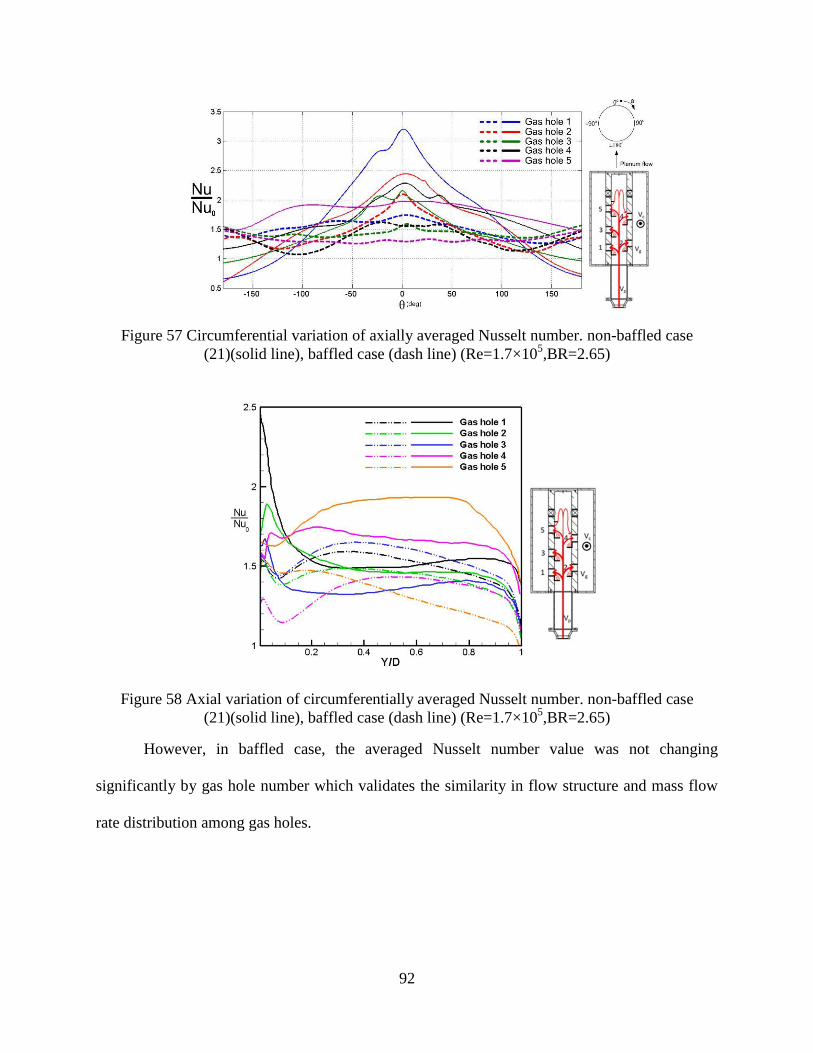
92
Figure 57 Circumferential variation of axially averaged Nusselt number. non-baffled case
(21)(solid line), baffled case (dash line) (Re=1.7×10⁵,BR=2.65)
Figure 58 Axial variation of circumferentially averaged Nusselt number. non-baffled case
(21)(solid line), baffled case (dash line) (Re=1.7×10⁵,BR=2.65)
However, in baffled case, the averaged Nusselt number value was not changing
significantly by gas hole number which validates the similarity in flow structure and mass flow
rate distribution among gas holes.
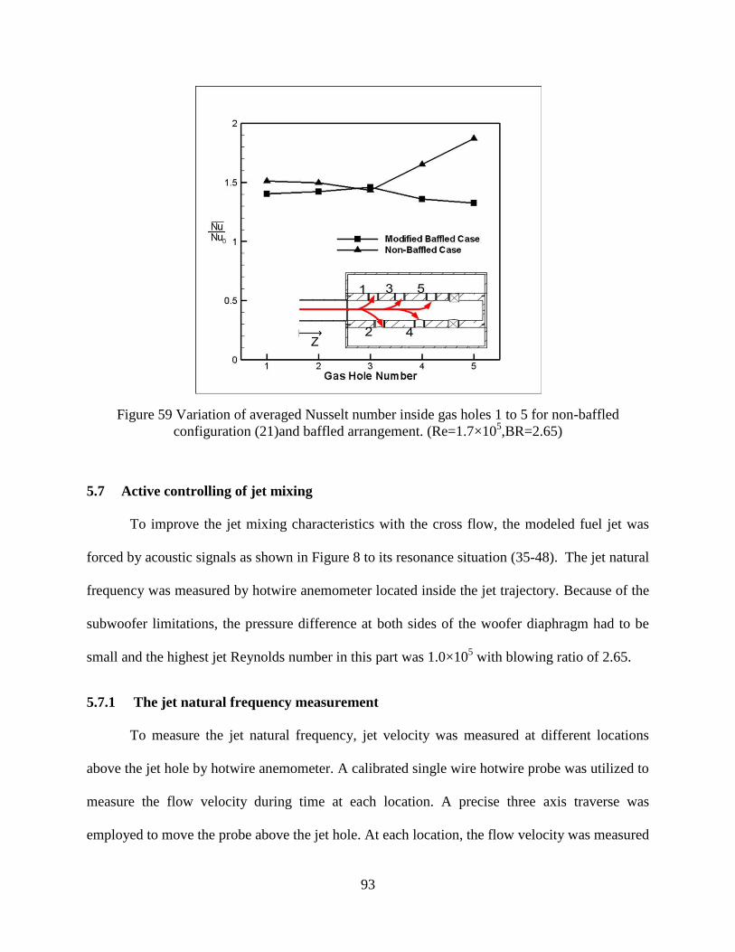
93
Figure 59 Variation of averaged Nusselt number inside gas holes 1 to 5 for non-baffled
configuration (21)and baffled arrangement. (Re=1.7×10⁵,BR=2.65)
5.7 Active controlling of jet mixing
To improve the jet mixing characteristics with the cross flow, the modeled fuel jet was
forced by acoustic signals as shown in Figure 8 to its resonance situation (35-48). The jet natural
frequency was measured by hotwire anemometer located inside the jet trajectory. Because of the
subwoofer limitations, the pressure difference at both sides of the woofer diaphragm had to be
small and the highest jet Reynolds number in this part was 1.0×10⁵ with blowing ratio of 2.65.
5.7.1 The jet natural frequency measurement
To measure the jet natural frequency, jet velocity was measured at different locations
above the jet hole by hotwire anemometer. A calibrated single wire hotwire probe was utilized to
measure the flow velocity during time at each location. A precise three axis traverse was
employed to move the probe above the jet hole. At each location, the flow velocity was measured
94
during 60 seconds. The velocity power spectrum was plotted at each location and the jet natural
frequency was calculated from the averaged value at different elevations above the jet hole. In
Figure 60, the velocity magnitude contour plots above the jet hole are presented. The jet hole exit
plane is located at the surface of L/D=0.0 and jet center is at (0, 0). As presented in Figure 60,
the velocity profile at the exit of the jet hole is completely non-uniform with a high speed region
favored to the aft side of the jet hole. The plenum flow direction is shown by the red arrow at the
bottom of the image and tunnel flow direction by the black arrow at the top. The low speed
region at the elevation of L/D=0.0 validates the recirculation bubble existence at the fore-side of
the jet hole. By elevating from the jet exit plane, the velocity magnitude decreases due to the jet
spreading downstream the jet hole. It can be seen that due to the non-symmetrical distribution of
velocity values at the jet exit plane, the jet velocity profile at L/D greater than 0 keeps the shape
as well. Also, the jet trajectory shape can be seen in Figure 60 as the peak velocity location
moves along the cross flow by moving away from the jet exit plane.
To find out the jet natural frequency, velocity power spectrum at each point on the
measurement grid was calculated. Figure 61 shows the velocity magnitude power spectrum
versus Strouhal number at three different elevations above the jet exit plane. The Strouhal
number was defined based on the jet hole diameter and the average velocity at the jet exit plane.
To achieve the Figure 61, velocity measurement was performed along a line at x=0.5 and y=0.0.
As presented in Figure 61, the peak frequency is larger near the jet exit plane comparing to other
locations. At the jet exit plane, the shear stresses are larger due to the strong velocity gradient
between the jet and cross flow. However, by elevating from the test section velocity magnitude
decreases and shear layer strength diminishes. The size of turbulent structures increases as the jet
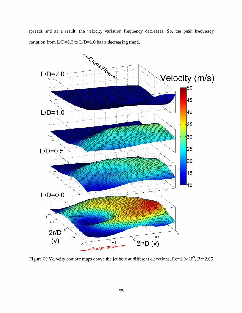
95
spreads and as a result, the velocity variation frequency decreases. So, the peak frequency
variation from L/D=0.0 to L/D=1.0 has a decreasing trend.
Figure 60 Velocity contour maps above the jet hole at different elevations, Re=1.0×10⁵, Br=2.65
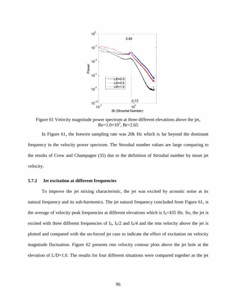
96
Figure 61 Velocity magnitude power spectrum at three different elevations above the jet,
Re=1.0×10⁵, Br=2.65
In Figure 61, the hotwire sampling rate was 20k Hz which is far beyond the dominant
frequency in the velocity power spectrum. The Strouhal number values are large comparing to
the results of Crow and Champagne (35) due to the definition of Strouhal number by mean jet
velocity.
5.7.2 Jet excitation at different frequencies
To improve the jet mixing characteristic, the jet was excited by acoustic noise at its
natural frequency and its sub-harmonics. The jet natural frequency concluded from Figure 61, is
the average of velocity peak frequencies at different elevations which is f0=435 Hz. So, the jet is
excited with three different frequencies of f0, f0/2 and f0/4 and the rms velocity above the jet is
plotted and compared with the un-forced jet case to indicate the effect of excitation on velocity
magnitude fluctuation. Figure 62 presents rms velocity contour plots above the jet hole at the
elevation of L/D=1.0. The results for four different situations were compared together as the jet

97
was perturbed with three different frequencies and also un-perturbed jet. The jet natural
frequency is indicated by f0 and f0/2 and f0/4 are the sub-harmonics of the jet natural frequency.
Figure 62 RMS velocity at L/D=1.0 above the jet hole for three different excitation frequency,
Re=1.0×10⁵, Br=2.65
As exhibited in Figure 62, the rms velocity distribution for un-perturbed jet and perturbed
jet with f0 are very similar. So, the difference in mixing characteristics of these two situations can
be neglected. However, for the jet perturbed with subharmonics of its natural frequency, the rms
velocity values are larger and indicate a better jet mixing with cross flow comparing to the
unperturbed jet. As presented, by perturbing the flow with f0/4, the rms velocity values are the
highest among all different situations. In this case, the rms velocity has been increased not only
above the jet hole, but also further downstream the jet hole. Also, the location of the pick rms
velocity was favored to the leading side of the jet (Y=-1) while the jet was perturbed by f0/4. In
contrast, the pick rms velocity region was favored to Y=+1 for other perturbed situations.
5.7.2.1 Mean velocity measurement
The mean jet velocity at different perturbation cases was measured by employing Particle
Image Velocimetry (PIV). The jet was seeded by Sub-micron olive oil particles and the PIV
sampling rate was 15 frames per second. Figure 63 exhibits the vertical jet velocity perpendicular
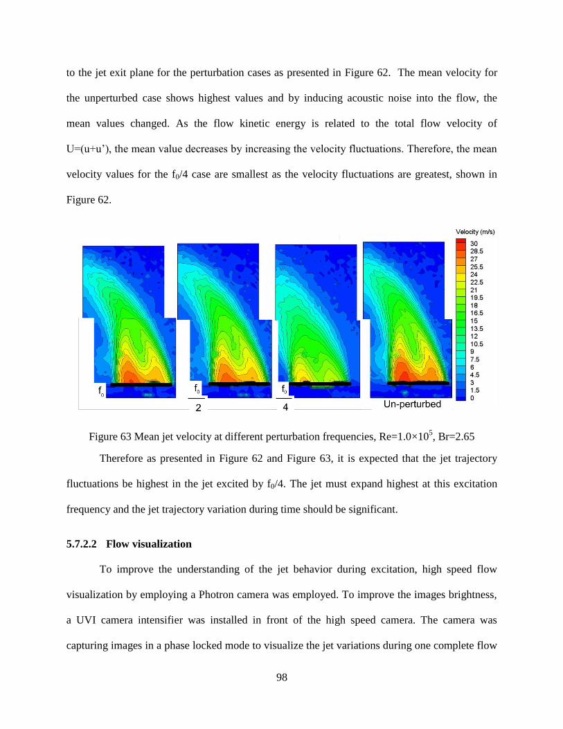
98
to the jet exit plane for the perturbation cases as presented in Figure 62. The mean velocity for
the unperturbed case shows highest values and by inducing acoustic noise into the flow, the
mean values changed. As the flow kinetic energy is related to the total flow velocity of
U=(u+u’), the mean value decreases by increasing the velocity fluctuations. Therefore, the mean
velocity values for the f0/4 case are smallest as the velocity fluctuations are greatest, shown in
Figure 62.
Figure 63 Mean jet velocity at different perturbation frequencies, Re=1.0×10⁵, Br=2.65
Therefore as presented in Figure 62 and Figure 63, it is expected that the jet trajectory
fluctuations be highest in the jet excited by f0/4. The jet must expand highest at this excitation
frequency and the jet trajectory variation during time should be significant.
5.7.2.2 Flow visualization
To improve the understanding of the jet behavior during excitation, high speed flow
visualization by employing a Photron camera was employed. To improve the images brightness,
a UVI camera intensifier was installed in front of the high speed camera. The camera was
capturing images in a phase locked mode to visualize the jet variations during one complete flow
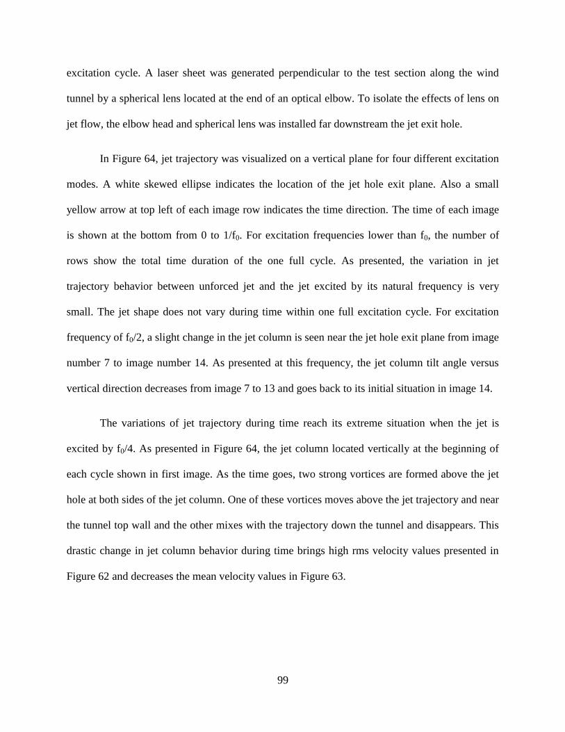
99
excitation cycle. A laser sheet was generated perpendicular to the test section along the wind
tunnel by a spherical lens located at the end of an optical elbow. To isolate the effects of lens on
jet flow, the elbow head and spherical lens was installed far downstream the jet exit hole.
In Figure 64, jet trajectory was visualized on a vertical plane for four different excitation
modes. A white skewed ellipse indicates the location of the jet hole exit plane. Also a small
yellow arrow at top left of each image row indicates the time direction. The time of each image
is shown at the bottom from 0 to 1/f0. For excitation frequencies lower than f0, the number of
rows show the total time duration of the one full cycle. As presented, the variation in jet
trajectory behavior between unforced jet and the jet excited by its natural frequency is very
small. The jet shape does not vary during time within one full excitation cycle. For excitation
frequency of f0/2, a slight change in the jet column is seen near the jet hole exit plane from image
number 7 to image number 14. As presented at this frequency, the jet column tilt angle versus
vertical direction decreases from image 7 to 13 and goes back to its initial situation in image 14.
The variations of jet trajectory during time reach its extreme situation when the jet is
excited by f0/4. As presented in Figure 64, the jet column located vertically at the beginning of
each cycle shown in first image. As the time goes, two strong vortices are formed above the jet
hole at both sides of the jet column. One of these vortices moves above the jet trajectory and near
the tunnel top wall and the other mixes with the trajectory down the tunnel and disappears. This
drastic change in jet column behavior during time brings high rms velocity values presented in
Figure 62 and decreases the mean velocity values in Figure 63.
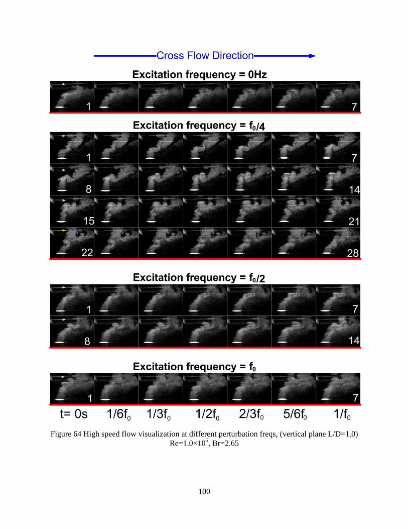
100
Figure 64 High speed flow visualization at different perturbation freqs, (vertical plane L/D=1.0)
Re=1.0×10⁵, Br=2.65
101
In Figure 65, the vortex formation mechanism above the jet column is exhibited more in detail.
As indicated by the red circle, it can be observed that from the image 6 in Figure 65, a small
vortex initiates inside the red circle. The vortex moves upward as it moves with the cross flow
and increases in size. In image 9, this vortex is located above the column and mixes with the jet
column in that location in image 10. From image number 11, this vortex is mixed with the jet and
its size became larger. Then, a big structure is formed in image 14 and moves upward to the top
of the tunnel. As this structure moves forward and upward simultaneously, it touches the tunnel
top wall in image 21 and moves down the tunnel until the new excitation cycle begins. As shown
in Figure 65, the vortex touches the tunnel wall at 0.15D downstream the jet hole.
Figure 65 Vortex formation above the jet column for perturbation frequency of f0/4
In a similar investigation for perturbation frequency of f0/2, Figure 66 presents that a
vortex was formed at the top side of the jet trajectory in image 5 and develops by moving down
the tunnel in image 13. It can be seen that this vortex moves forward and touches the tunnel top
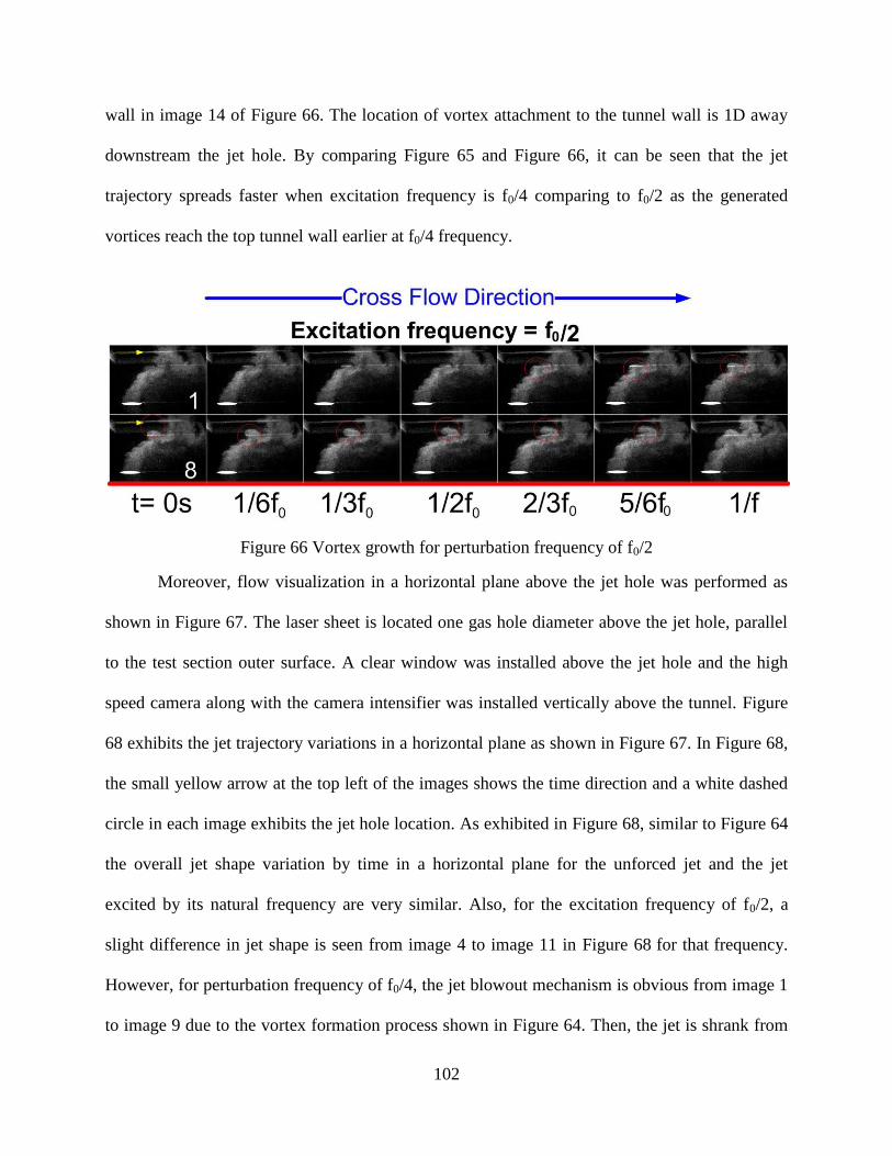
102
wall in image 14 of Figure 66. The location of vortex attachment to the tunnel wall is 1D away
downstream the jet hole. By comparing Figure 65 and Figure 66, it can be seen that the jet
trajectory spreads faster when excitation frequency is f0/4 comparing to f0/2 as the generated
vortices reach the top tunnel wall earlier at f0/4 frequency.
Figure 66 Vortex growth for perturbation frequency of f0/2
Moreover, flow visualization in a horizontal plane above the jet hole was performed as
shown in Figure 67. The laser sheet is located one gas hole diameter above the jet hole, parallel
to the test section outer surface. A clear window was installed above the jet hole and the high
speed camera along with the camera intensifier was installed vertically above the tunnel. Figure
68 exhibits the jet trajectory variations in a horizontal plane as shown in Figure 67. In Figure 68,
the small yellow arrow at the top left of the images shows the time direction and a white dashed
circle in each image exhibits the jet hole location. As exhibited in Figure 68, similar to Figure 64
the overall jet shape variation by time in a horizontal plane for the unforced jet and the jet
excited by its natural frequency are very similar. Also, for the excitation frequency of f0/2, a
slight difference in jet shape is seen from image 4 to image 11 in Figure 68 for that frequency.
However, for perturbation frequency of f0/4, the jet blowout mechanism is obvious from image 1
to image 9 due to the vortex formation process shown in Figure 64. Then, the jet is shrank from
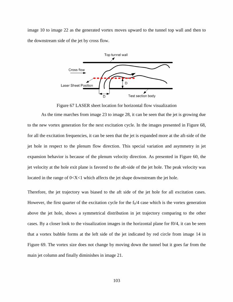
103
image 10 to image 22 as the generated vortex moves upward to the tunnel top wall and then to
the downstream side of the jet by cross flow.
Figure 67 LASER sheet location for horizontal flow visualization
As the time marches from image 23 to image 28, it can be seen that the jet is growing due
to the new vortex generation for the next excitation cycle. In the images presented in Figure 68,
for all the excitation frequencies, it can be seen that the jet is expanded more at the aft-side of the
jet hole in respect to the plenum flow direction. This special variation and asymmetry in jet
expansion behavior is because of the plenum velocity direction. As presented in Figure 60, the
jet velocity at the hole exit plane is favored to the aft-side of the jet hole. The peak velocity was
located in the range of 0<X<1 which affects the jet shape downstream the jet hole.
Therefore, the jet trajectory was biased to the aft side of the jet hole for all excitation cases.
However, the first quarter of the excitation cycle for the f0/4 case which is the vortex generation
above the jet hole, shows a symmetrical distribution in jet trajectory comparing to the other
cases. By a closer look to the visualization images in the horizontal plane for f0/4, it can be seen
that a vortex bubble forms at the left side of the jet indicated by red circle from image 14 in
Figure 69. The vortex size does not change by moving down the tunnel but it goes far from the
main jet column and finally diminishes in image 21.
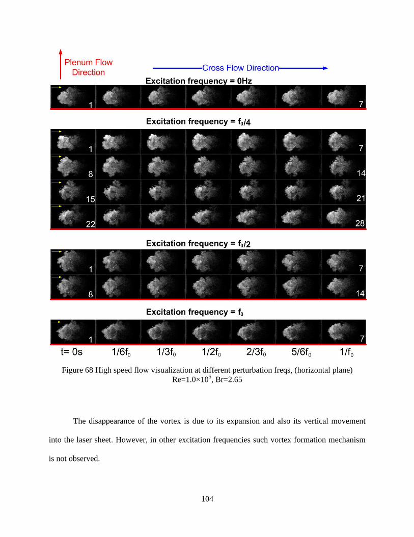
104
Figure 68 High speed flow visualization at different perturbation freqs, (horizontal plane)
Re=1.0×10⁵, Br=2.65
The disappearance of the vortex is due to its expansion and also its vertical movement
into the laser sheet. However, in other excitation frequencies such vortex formation mechanism
is not observed.
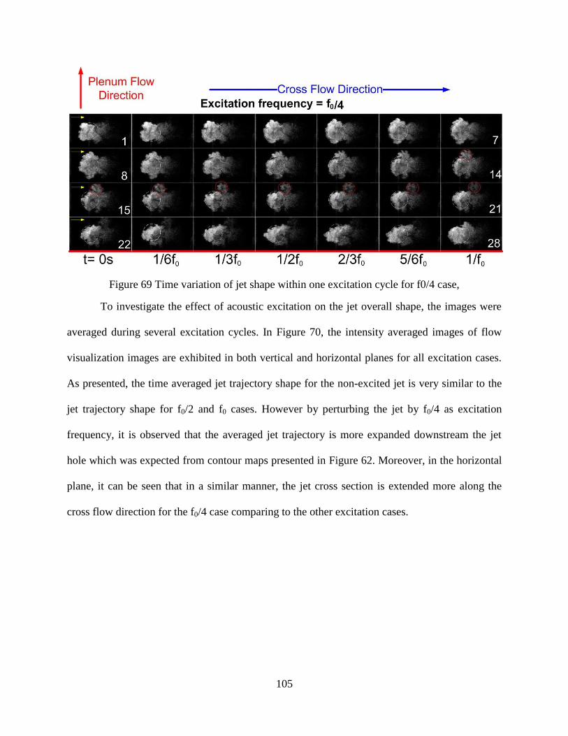
105
Figure 69 Time variation of jet shape within one excitation cycle for f0/4 case,
To investigate the effect of acoustic excitation on the jet overall shape, the images were
averaged during several excitation cycles. In Figure 70, the intensity averaged images of flow
visualization images are exhibited in both vertical and horizontal planes for all excitation cases.
As presented, the time averaged jet trajectory shape for the non-excited jet is very similar to the
jet trajectory shape for f0/2 and f0 cases. However by perturbing the jet by f0/4 as excitation
frequency, it is observed that the averaged jet trajectory is more expanded downstream the jet
hole which was expected from contour maps presented in Figure 62. Moreover, in the horizontal
plane, it can be seen that in a similar manner, the jet cross section is extended more along the
cross flow direction for the f0/4 case comparing to the other excitation cases.
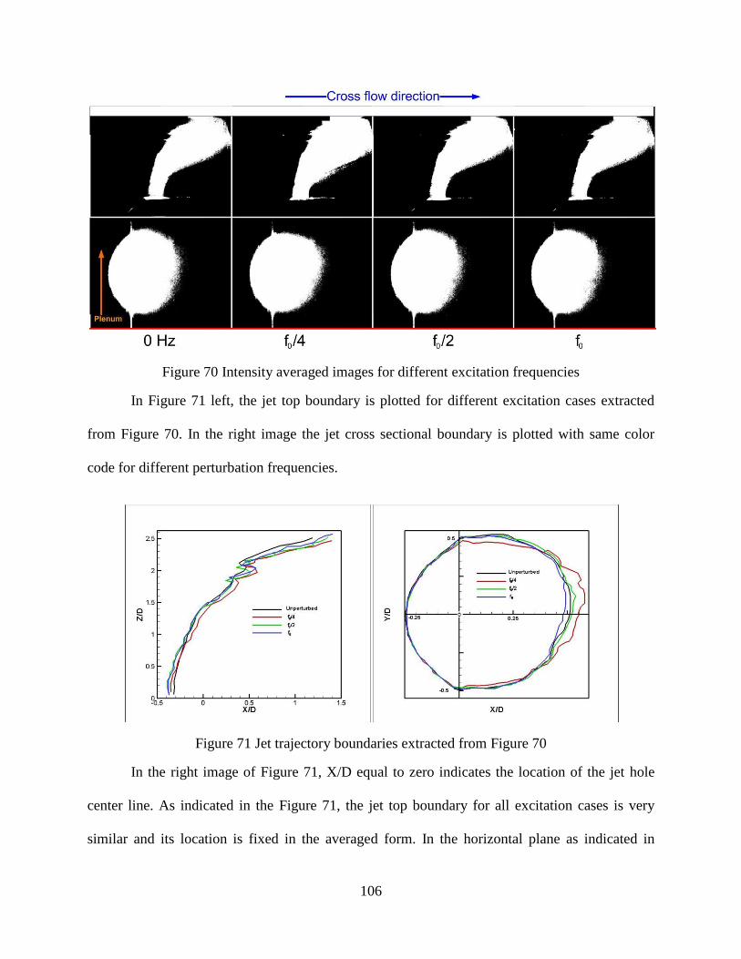
106
Figure 70 Intensity averaged images for different excitation frequencies
In Figure 71 left, the jet top boundary is plotted for different excitation cases extracted
from Figure 70. In the right image the jet cross sectional boundary is plotted with same color
code for different perturbation frequencies.
Figure 71 Jet trajectory boundaries extracted from Figure 70
In the right image of Figure 71, X/D equal to zero indicates the location of the jet hole
center line. As indicated in the Figure 71, the jet top boundary for all excitation cases is very
similar and its location is fixed in the averaged form. In the horizontal plane as indicated in

107
Figure 71, the jet cross section is extended more along the cross flow for f0/4 case which
validates the jet expansion at that excitation frequency. On the other hand, for the unperturbed
jet, f0/2 and f0 cases the jet cross sectional area does not vary significantly which was exhibited
in Figure 70.

108
Chapter 6: Conclusion
The heat transfer coefficient and flow structure inside fuel premixing devices were
investigated experimentally and numerically. The effect of Reynolds number, blowing ratio and
hole configuration on the heat transfer inside the gas holes were investigated. Pressure and
velocity measurements inside each hole were performed for improved understanding of the in-
hole heat transfer contour maps. Moreover, to reduce the thermal stresses intensity inside the
device, straight baffles of different height were placed upstream of cooling holes inlet inside the
plenum. Results were compared with basic geometry as studied by Acharya et al (21). Flow field
was simulated numerically using FLUENT to improve the understanding of velocity profile
inside cooling holes and verified by experimental measurements. The following major
conclusions were made from this study:
The flow entering the first three holes of all configurations impinges the aft-side of the
holes. The resulting heat transfer coefficient and Nu value is very high at the
impingement point with peak Nu/Nuo generally in the range of 4-8.
For gas holes 1-3, the flow turning and impingement on the aft-side is associated with
flow separation on the leading side of the hole where Nu/Nuo values are low (<1).
For gas holes closest to the end of the feed tube (holes 4 and 5 for configuration (A), the
flow into the gas hole is more symmetric leading to more uniform Nu distributions.
The local heat transfer distribution inside gas holes changes from a highly non-uniform
circumferential distribution inside hole 1 to a nearly uniform distribution in hole 5.
Among all four different hole configurations, arrangement (D) exhibits lower averaged
heat transfer values from 1st to 5
th hole.
The blowing ratio does not affect the heat transfer coefficient inside the holes.

109
Flow structure inside cooling holes can be easily manipulated by modifying the plenum
geometry
Placing baffles upstream cooling holes vanishes the recirculation bubble at the fore side
of cooling holes inlet while baffle height is same as baffle distance from cooling hole
inlet.
The recirculation bubble at the back side of baffles guides air to flow smoothly into
cooling holes downstream of baffles.
Using baffles with variable height distributes mass flow rate through cooling holes more
uniformly.
In modified plenum geometry, heat transfer coefficient inside holes was distributed more
uniform comparing to basic plenum. The difference between maximum and minimum
Nusselt numbers was decreased by modifying the plenum design.
The jet mixing characteristics and trajectory can be manipulated by forcing the jet with
sound waves.
Perturbing the jet by sound wave at one fourth of the jet natural frequency improves the
jet mixing and expands the jet column most comparing to the unperturbed jet.

110
Works Cited
1. Bejan, Adrian. Convection Heat Transfer. New York : John Wiley & Sons, 2004.
2. Turbulent heat transfer in the entrance region of a tube. Alarabi, M. 3-4, 1982, Heat Transfer
Engineering, Vol. 3.
3. Heat transfer measurement and correlations in the transient region for a circular tube with
three different inlet configurations. Ghajar, A,J and Tam, L, M. 1994, experimental thermal
and fluid science, Vol. 8.
4. Turbulent heat transfer in a symmetrically or asymmetrically heated flat rectangular duct with
flow separation at inlet. Sparrow, E, M and Cur, N. febreuary 1982, Journal of heat transfer,
Vol. 104.
5. Developing heat transfer in rectangular channels with rib turbulators”, International journal
of heat and mass transfer. Han, J, C and Park, J, S. 1, 1988, International journal of heat and
mass transfer, Vol. 31.
6. Application of linear and non-linear low-Re k-ε models in two dimensional predictions of
convective heat transfer in passages with sudden contractions. Raisee, M and Hejazi, S, H.
2007, International journal of heat and fluid flow, Vol. 28.
7. Turbulent forced convection flow adjacent to inclined forward step in a duct. Ganjalikhan
Nassab, S, A, Moosavi, R and Hosseini Sarvari, S, M. 2009, International journal of thermal
sciences, Vol. 48.
8. Experimental mass(heat) transfer in and near a circular hole in a flat plate. Cho, H, H,
Jabbari, M, Y and Goldstein, R, J. 10, 1997, International Journal of heat and mass transfer,
Vol. 40.
9. Heat (mass) transfer and film cooling effectiveness with injection through discrete holes: part
I-Within holes and the back surface. Cho, H, H and Goldstein, R, J. 1995, Vol. 117.
10. Heat/Mass transfer measurement within a film cooling hole of square and rectangular cross
section. Cho, H, H, Kang, S, G and Rhee, D, H. 2001, Journal of turbomachinery, Vol. 123.
11. Effect of plenum crossflow on heat (mass) transfer near and within the entrance of film
cooling holes. Goldstein, R, J, Cho, H, H and Jabbari, M, Y. 1997, Journal of
Turbomachinery, Vol. 119.
12. Short hole jet in crossflow velocity field and its relationship to film cooling performance.
Peterson, S, D and Plesniak, M, W. 2002, Experiments in Fluid, Vol. 33.
13. 3-D simulation of dividing flows in 90 deg rectangular closed conduits. Ramamurthy, A, S,
et al. 2006, Journal of fluids engineering, Vol. 128.

111
14. The Influence of Coolant Supply Geometry on Film Coolant Exit Flow and Surface Adiabatic
Effectiveness. Burd, S, W and Simon, T, W. s.l. : ASME, 1997. 97-GT-25.
15. Film Cooling Effectiveness for short Film Cooling Holes Fed by a Narrow Plenum. Hale, C,
A, Plesniak, M, W and Ramadhyani, S. 2000, ASME journal of turbomachinery, Vol. 122, pp.
553-557.
16. A Systematic Study of the Aerodynamics of Leading Edge Film Cooling on a Large Scale
High Pressure Turbine Cascade. Ardey, S and Fottner, L. s.l. : ASME, 1998. 98-GT-434.
17. Numerical simulation and aerothermal physics of leading edge film cooling.
Chernobrovkin, A and Lakshminarayana, B. s.l. : ASME, 1998. 98-GT-504.
18. Discrete-jet film cooling: a comparison of computational results with experiments. Leylek, J,
H and Zerkle, R, D. s.l. : ASME, 1994, Journal of turbomachinery, Vol. 116, pp. 358-368.
19. Vortex generating flow passage design for increased film-cooling effectiveness and surface
coverage. Papell, S, S. s.l. : NASA, 1984, Technical Memorandum, Vol. 83617.
20. Film cooling effectiveness downstream of a single row of holes with variable density ratio.
Sinha, A, K, Bogard, D, G and Crawford, M, E. s.l. : ASME, 1991, Journal of
turbomachinery, Vol. 113, pp. 442-449.
21. Flow distribution and heat transfer coefficients inside gas holes discharging into an
orthogonal cross-flow. Acharya, S, Eshtiaghi, A, H and Schilp, R. Vancouver, BC : ASME,
2011. IGTI conference.
22. Influence of internal flow on film cooling effectiveness. Wilfert, G and Wolf, S. s.l. : ASME,
April 2000, Journal of Turbomachinery, Vol. 122.
23. Numerical Investigation of the Influence of Specific Vortex Generation on the Mixing
Process of Film Cooling Jets. Vogel, D, T. s.l. : ASME, 1998. 98-GT-210.
24. ‘Flowfield Measurements for Film-Cooling Holes With Expanded Exits. Thole, K, et al. s.l. :
ASME, 1998, journal of turbomachinery, Vol. 120, pp. 327-336.
25. Heat Transfer Coefficient Measurement of Film-Cooling Holes With Expanded Exits.
Gritsch, M, Schulz, A and Wittig, S. s.l. : ASME, 1998. 98-GT-28.
26. A Numerical Study of Discrete-Hole film cooling. Berhe, M, K and Patankar, S, V. s.l. :
ASME, 1996. WA/HAT-8.
27. An advanced impingement/film cooling scheme for gas turbines- numerical study.
Immarigeon, A and Hassan, I. 4, 2006, Intenational journal of numerical methods for heat &
fluid flow, Vol. 16.

112
28. INFLUENCE OF INTERNAL CYCLONE FLOW ON ADIABATIC FILM COOLING
effectiveness. Lerch, A and Schiffer, H, P. Antalya, turkey : s.n., 2009. International
Symposium on Heat Transfer in Gas Turbine Systems.
29. On density effects and large structure in turbulent mixing layers. Brown, G, L and Roshko,
A. 1974, Journal of Fluid Mechanic, Vol. 64, pp. 715-816.
30. Vortex pairing: the mechanism of turbulent mixing-layer growth at moderate Reynolds
number. Winant, C, D and Browand, F, K. 1974, Journal of Fluid Mechanic, Vol. 63, pp. 237-
252.
31. Subharmonics and vortex merging in mixing layers. Ho, C,M and Huang, L,S. 1982,
Journal Of Fluid Mechanic, Vol. 119, pp. 443-473.
32. Streamwise vortex structure in plane mixing layers. Bernal, L, P and Roshko, A. 1986,
journal of fluid mechanic, Vol. 170, pp. 499-525.
33. Helical instabilities of slowly divergent jets. Plaschko, P. 1979, Journal of fluid mechanic,
Vol. 92, pp. 209-215.
34. On spatially growing disturbances in an inviscid shear layer. Michalke, A. 1965, Journal of
fluid mechanic, Vol. 23, pp. 521-544.
35. Orderly structure in jet turbulence. Crow, S and Champagne, F. 1971, Journal of Fluid
mechanic, Vol. 48, pp. 547-591.
36. Vortex pairing in a circular jet under controlled excitation. Part 1. General jet response.
Zaman, K, B, M, Q and Hussain, A, K, M, F. 1980, Journal of Fluid mechanic, Vol. 101, pp.
449-491.
37. The effect of forcing on the mixing-layer region of a round jet. Reynolds, W. C and
Bouchard, E, E,. berlin : springer, 1981. Unsteady turbulent shear flows. pp. 402-411.
38. Control of an axisymmetric jet using vortex generators. Zaman, K, B, Reeder, M, F and
Samimy, M. 1994, Physics of Fluids, Vol. 6, pp. 778-793.
39. Study of jets from rectangular nozzles with square grooves. Kumar, P, et al. 2011,
Aeronautical Journal, Vol. 115, pp. 187-196. 0001-9240.
40. Effects of nozzle-exit boundary-layer conditions on excitability of heated free jets.
Lepicovsky, J and Brown, W, H. 1989, AIAA journal, Vol. 27, pp. 712-718.
41. Heat transfer and flow structures in an excited circular impinging jet. Liu, T and Sullivan,
J, P. 1996, International Journal of heat and mass transfer, Vol. 39, pp. 3695-3706.
113
42. Periodic Excitation for Jet Vectoring and Enhanced Spreading. Pack, L, G and Seifert, A.
3, 2001, Journal of Aircraft, Vol. 38, pp. 486-495.
43. Vortex interaction and mixing in a driven gaseous axisymmetric jet. Meyer, T, R, Dutton, J,
C and Lucht, R, P. November 1999, Physics of fluid, Vol. 11.
44. The actively controlled jet in crossflow. M'Closkey, R, T, et al. 2002, Journal of Fluid
mechanic, Vol. 452, pp. 325-335.
45. Effects of acoustic excitation positions on heat transfer and flow in axisymmetric impinging
jet: main jet excitation and shear layer excitation. Hwang, S, D and Cho, H, H. october 2003,
International journal of heat and fluid flow, Vol. 24, pp. 199-209.
46. Heat transfer to an acoustically excited impinging air jet. O'Donovan, T,S and Murray, D,
B. Netherlands : s.n., 2008. 5th European Thermal-Sciences Conference.
47. Direct Numerical Simulation of pulsed jets-in-crossflow. Muldoon, F and Acharya, S.
2010, Computers and Fluids, Vol. 39, pp. 1745-1773.
48. Experimental investigation of the flow and heat transfer of an impinging jet under acoustic
excitation. Roux, S, et al. 2011, International journal of heat and mass transfer, Vol. 54, pp.
3277-3290.
49. Delrin Acetal resin, Design guide-Module. www.Dupont.com. [Online]
50. Miniature five-hole pressure probe for measurement of three mean velocity components in
low-speed flows. Ligrani, P, M, Singer, B, A and Baun, L, R. 1989, Journal of physics,
scientific instruments, Vol. 22.
51. Describing experimental uncertainties in single sample experiments. Kline, S, J and
McClintock, F, A. 1953, Mechanical Engineering, Vol. 75.
52. OMEGA revised thermocouple reference tables. [Online] Omega.
53. Johnson, B, V and Wagner, J, H. Heat transfer experiments in the internal cooling
passages of a cooled radial turbine rotor. contractor report, NASA. 1996.
54. FLUENT user manual. s.l. : FLUENT inc.
55. prediction of axisymmetric and two-dimensional impinging turbulent jets. Dianat, M,
Fairweather, M and Jones, W, P. 1996, international journal of heat and fluid flow, Vol. 17.
56. Influence of internal flow on film cooling effectiveness. Wilfert, G and Wolf, S. s.l. : ASME,
April 2000, Journal of Turbomachinery, Vol. 122.

114
57. Numerical Investigation of the influence of specific vortex generation on the mixing process
of film cooling jets. Vogel, D, T. s.l. : ASME, 1998. IGTI. Vols. 98-GT-210.
58. Film cooling effectiveness downstream of a single row of holes with variable density ratio.
Sinha, A, K, Bogard, D, G and Crawford, M, E. s.l. : ASME, 1991, Journal of
Turbomachinery, Vol. 113, pp. 442-449.
59. Papel, S, S. Vortex Generating flow passage design for increased film-cooling effectiveness
and surface coverage. Technical Memorandum. s.l. : NASA, 1984.
60. Discrete Jet film cooling: A comparison of computational results with experiments. Leylek,
J, H and Zerkle, R, D. s.l. : ASME, 1994, Journal of Turbomachinery, Vol. 116, pp. 358-368.
61. Numerical Simulation and Aerothermal physics of leading edge film cooling.
Chernobrovkin, A and Lakshminarayana, B. s.l. : ASME, 1998. IGTI. Vols. 98-GT-504.
62. A systematic study of the aerodynamics of leading edge film cooling on a large scale high
pressure turbine cascade. Aredy, S and Fottner, L. 1998. IGTI. Vols. 98-GT-434.
63. Flow Distribution and Heat Transfer Coefficients inside Gas Holes Discharging into an
Orthogonal Crossflow. Acharya, S, Eshtiaghi, A,H and Schilp, R. Vancouver, CA : ASME,
2011. IGTI. Vols. GT2011-46854.
64. Detailed heat transfer distributions in two-pass square channels with rib turbulators and
bleed holes . Ekkad, S V, Huang, Y and C, Han J. 23, 1998, International Journal of Heat and
Mass Transfer, Vol. 41.

115
Vita
Amirhossein Eshtiaghi was born in Tehran, Iran, in Provence from the union of Hassan
Eshtiaghi and Fereshteh Ghanbari in May 1983.
He obtained his bachelorette with honors in September 2005 at the University of Tehran,
Iran. He then joined Shiraz University for Masters Program for three years under supervision of
Prof. M. Yaghoubi. He submitted his research named Experimental and Numerical investigation
on natural convection from cylinders located beneath an adiabatic surface on May 2008.
He entered the Louisiana State University in January 2009 to get a new Masters degree under the
supervision of Dr. Sumanta Acharya in the department of Mechanical Engineering. He
submitted his research named Flow distribution and heat transfer coefficients inside gas holes
discharging orthogonally into a cross flow to graduate in August 2012.