Theor Ecol (2008) 1:153–161DOI 10.1007/s12080-008-0016-2

ORIGINAL PAPER

Floquet theory: a useful tool for understandingnonequilibrium dynamics

Christopher A. Klausmeier

Received: 5 October 2007 / Accepted: 4 February 2008 / Published online: 12 July 2008© Springer Science + Business Media B.V. 2008

Abstract Many ecological systems experience periodicvariability. Theoretical investigation of population andcommunity dynamics in periodic environments hasbeen hampered by the lack of mathematical tools rela-tive to equilibrium systems. Here, I describe one suchmathematical tool that has been rarely used in theecological literature but has widespread use: Floquettheory. Floquet theory is the study of the stability oflinear periodic systems in continuous time. Floquet ex-ponents/multipliers are analogous to the eigenvalues ofJacobian matrices of equilibrium points. In this paper,I describe the general theory, then give examples toillustrate some of its uses: it defines fitness of struc-tured populations, it can be used for invasion criteriain models of competition, and it can test the stability oflimit cycle solutions. I also provide computer code tocalculate Floquet exponents and multipliers.

Keywords Nonequilibrium dynamics · Floquet theory

Introduction

Populations, communities, and ecosystems vary intime, a truism obvious to natural historians (Thoreau

Electronic supplementary material The online version ofthis article (doi:10.1007/s12080-008-0016-2) containssupplementary material, which is available to authorizedusers.

C. A. Klausmeier (B)W. K. Kellogg Biological Station, Michigan State University,Hickory Corners, East Lansing, MI 49060, USAe-mail: klausme1@msu.edu

1854) and well-quantified by empiricists (Kratz et al.2003). The origin of these fluctuations can be exter-nal (e.g., weather) or internal (e.g., predator–preycycles), and the fluctuations can be random, periodic,or chaotic. Given the ubiquity of temporal variabilityand its potential importance for structuring ecologicalsystems, theoreticians have been eager to incorporateits effects in ecological models (Nisbet and Gurney1982; DeAngelis and Waterhouse 1987; Chesson 1994).Despite these efforts, we still do not have a full un-derstanding of the effect of temporal variability ontheoretical communities and ecosystems, much less realones. Why not?

First, temporal variability is a multifaceted phenom-enon with complex and idiosyncratic effects on differ-ent ecological processes. Details matter. For example,some models of competition have shown that fluctua-tions can increase diversity (Armstrong and McGehee1980; Chesson 1994; Litchman and Klausmeier 2001),while others have shown that they can decrease diver-sity (May 1974). The effect of environmental noise hasbeen showed to strongly depend on the spectrum of thenoise (Steele and Henderson 1984; Kaitala et al. 1997).

Second, nonequilibrium dynamics are more difficultto analyze mathematically than equilibrium situationsbecause fewer analytical tools are available. A numberof analytical techniques have been applied to ecologicalmodels, but each has a limited range of applicability.For example, Chesson’s decomposition of competitiveeffects in a stochastic environment (Chesson 1994)and Nisbet and Gurney’s use of transfer functions(Nisbet and Gurney 1982) both assume small envi-ronmental fluctuations. Elsewhere, we have developedtechniques that assume that environmental variability isslow compared to population dynamics (Litchman and

154 Theor Ecol (2008) 1:153–161

Klausmeier 2001; Klausmeier in preparation). Whenthese approximations are not valid, the typical ap-proach to studying nonequilibrium dynamics is bruteforce numerical solution of the model (e.g., Grover1991; Hastings and Powell 1991; Brassil 2006). All ofthese tools have their place in the theoretician’s tool-box, but we could use more of them.

In this paper, I explain and illustrate one such tool:Floquet theory. Although Floquet theory has a widerange of potential uses in ecological and evolutionarymodeling and is relatively easy to implement, its use inecology has been extremely limited (Kooi and Troost2006). The mathematics here is not novel or particularlyadvanced; Floquet theory is typically taught in a secondcourse on ordinary differential equations (cf. Drazin1992; Grimshaw 1993; Strogatz 1994). However, mostecologists do not take one, much less two, coursesin differential equations. Instead, they learn modelingtechniques from a course in theoretical ecology, whichtypically do not incorporate Floquet theory (cf. Nisbetand Gurney 1982; Yodzis 1989; Hastings 1997). Giventhe potential utility of Floquet theory, its lack of useindicates that it needs better advertising. Therefore,the goal of this paper is to promote the wider use ofFloquet theory as a useful tool for studying the effectsof temporal variability on ecological systems.

What is Floquet theory? It is the study of linearsystems of differential equations with periodic coeffi-cients. What can you do with it? You can use it foranything you would use linear stability analysis for,when dealing with a periodic system. In particular,it has three potentially important uses in ecologicaltheory: 1) defining fitness of structured populations inperiodic environments, 2) calculating invasion criteriafor interacting structured populations in periodic envi-ronments, and 3) testing the stability of a limit cycle.A structured population is one that can not be mod-eled as a single state variable. Some different types ofpopulation structure are physiological structure (Metzand Diekmann 1986), age and stage structure (Caswell2001), and spatial structure (Tilman and Kareiva 1997).

In the remainder of this paper, I outline the ideasbehind Floquet theory. I describe a numerical methodfor calculating Floquet multipliers and define a Math-ematica (Wolfram Research Inc. 2007) function to dothis calculation. Then, I give three ecological examplesof the utility of Floquet theory. First, I explore theevolution of dispersal in a two-patch metapopulationwith spatiotemporal fluctuations. Second, I calculate in-vasion criteria in a model of competing stage-structuredpopulations in a seasonal environment. Third, I calcu-late the stability of a limit cycle in a tri-trophic food

chain model (Hastings and Powell 1991). Finally, Isuggest other applications of Floquet theory and de-scribe its generalization to environments with aperiodictemporal variation (Metz et al. 1992).

Theory

Here, I largely follow Grimshaw (1993); the readerwho wants more details could consult it or anotherdifferential equations text (e.g., Drazin 1992; Strogatz1994). Consider a set of linear, homogeneous, time-periodic differential equations

dxdt

= A(t)x (1)

where x is a n-dimensional vector and A(t) is an n × nmatrix with minimal period T. Although its parame-ters A(t) vary periodically, the solutions of Eq. 1 aretypically not periodic, and despite its linearity, closed-form solutions of Eq. 1 typically cannot be found. Thegeneral solution of Eq. 1 takes the form

x(t) =n∑

i

cieμi tpi(t) (2)

where ci are constants that depend on initial conditions,pi(t) are vector-valued functions with period T, and μi

are complex numbers called characteristic or Floquetexponents. Characteristic or Floquet multipliers arerelated to the Floquet exponents by the relationshipρi = eμiT . As can be seen from Eq. 2, the solution toEq. 1 is the sum of n periodic functions multiplied byexponentially growing or shrinking terms. The long-term behavior of the system is determined by the Flo-quet exponents. The zero equilibrium is stable if allFloquet exponents have negative real parts or, equiv-alently, all Floquet multipliers have real parts between−1 and 1. If any Floquet exponent has a positive realpart (equivalent to a Floquet multiplier with modulusgreater than one), then the zero equilibrium is unsta-ble and ||x(t)|| → ∞ as t → ∞. Thus, Floquet expo-nents/multipliers can be interpreted in the same way aseigenvalues are in models with constant coefficients incontinuous/discrete time, respectively; they representthe growth rate of different perturbations averagedover a cycle. Floquet exponents are rates with unitstime−1, and Floquet multipliers are dimensionless num-bers that give the period-to-period increase/decrease ofthe perturbation.

Theor Ecol (2008) 1:153–161 155

How can Floquet exponents/multipliers be calcu-lated? While the eigenvalues of a matrix can becalculated analytically, Floquet exponents/multiplierstypically must be calculated numerically. An efficientapproach is available. Solve the matrix differentialequation

dXdt

= A(t)X (3)

over one period (from t = 0 to t = T), with the identitymatrix as an initial condition (X(0) = I). The matrixX(T) is known as a fundamental matrix (Grimshaw1993). Floquet multipliers, ρi, are the eigenvalues ofX(T) and Floquet exponents, μi can calculated as(log ρi)/T. Code to do these calculations in Mathe-matica (Wolfram Research, Inc. 2007) is supplied inthe Electronic Appendix, which should be easily imple-mented in other systems.

Example 1: fitness of structured populationsin periodic environments

Metz et al. (1992) showed that the general definition offitness is given by the asymptotic exponential growthrate, which is determined by the dominant Lyapunovexponent. Floquet exponents are the special case ofLyapunov exponents applied to continuous-time pe-riodic systems, so it follows that Floquet exponentsshould be useful in the evolutionary ecology of struc-tured populations. Frequency dependence can be in-corporated in a nonlinear model, calculating fitness asan invasion rate as in the next example (see also Metzet al. 1992; Kooi and Troost 2006).

Here, I give an example of the evolution of dispersalin a spatiotemporal mosaic environment. Consider apopulation that lives in two patches, with densitiesx1 and x2. In each patch, the population grows orshrinks exponentially at rate ri(t) with r1(t) = sin 2π tand r2(t) = − sin 2π t, so that the two patches changefrom sources (r > 0) to sinks (r < 0) perfectly out ofphase with period T = 1. The patches are coupledby random dispersal with rate d. The model for thissituation is

dx1

dt= r1(t)x1 + d (x2 − x1)

dx2

dt= r2(t)x2 + d (x1 − x2)

or, in the form of Eq. 1,

A(t) =(

r1(t) − d dd r2(t) − d

)(4)

Before calculating the asymptotic population growthrate (fitness) for arbitrary d, consider two special cases.

If the two patches are completely uncoupled (d = 0),then the growth rate in each patch varies from −1 to 1,with an average growth rate of zero. It is well known

a

b

c

Fig. 1 Population dynamics in two patches governed by Eqs. 1and 4 with different dispersal rates. Initial conditions: x1(0) = 1,x2(0) = 1. Solid line is density in patch 1, dotted line is density inpatch 2. a d = 0. b d = 104 (effectively infinite). c d = 3

156 Theor Ecol (2008) 1:153–161

that an isolated population growing exponentially in atime-varying environment grows according to its aver-age growth rate. Therefore, for d = 0, we expect no netgrowth or decline. A numerical solution of Eq. 1, withA(t) given by Eq. 4, shows this to be correct (Fig. 1a).Each subpopulation grows during the favorable part ofthe period and declines the exact same amount duringthe unfavorable part.

If the two patches are completely well-mixed(d = ∞), then we expect the population to experi-ence both patches equally, averaging growth rates overspace. Because the two patches are out-of-phase, thespatial-average growth rate is (r1 + r2)/2 = 0, so wewould again expect no net growth, this time without anyfluctuations. Again, the numerical solution of Eqs. 1and 4 with large d shows this to be correct (Fig. 1b).

Given the behavior of these two limiting cases andthe linearity of Eq. 1, one might expect no net growthfor any d. Numerical solution of Eqs. 1 and 4 shows thisto be incorrect; instead, the population grows withoutbound (Fig. 1c). Evaluating the maximum Floquet ex-ponent of Eq. 4 as a function of dispersal rate, d, verifiesthat these numerical results are correct (Fig. 2): netpopulation growth is zero for d = 0 and d = ∞, but itis positive for intermediate d. Figure 2 shows that thereis an optimal dispersal rate d that maximizes fitness; inthis case, it is d = 3.132, which leads to a growth rateof 0.03966. Thus, even with no explicit cost of dispersal,there is an optimal dispersal rate in a spatiotemporalmosaic environment. This is a simple example of thephenomenon of inflation recently introduced by Holtand colleagues (Gonzalez and Holt 2002; Holt et al.2003; Roy et al. 2005); it complements their work be-cause it considers multiple patches in continuous timeand with periodic variability, whereas existing workfocuses on a single patch (Gonzalez and Holt 2002;

Fig. 2 Dominant Floquet exponent as a function of dispersalrate, d. Fitness is maximized at an intermediate d = 3.132

Holt et al. 2003) or stochastic variability in discrete time(Roy et al. 2005).

Example 2: invasion criteria for interacting structuredpopulations

Invasion criteria are a powerful tool for analyz-ing pairwise competitive interactions (Armstrong andMcGehee 1980). Each species is grown in monoculture,then the other species is introduced at low density andits invasion rate is calculated. If species one invadesspecies two, but not vice versa, then we say species oneoutcompetes species two. If the reverse is true, speciestwo outcompetes species one. If each species can invadea monoculture of the other, then we say the two speciescoexist, and if neither species can invade a monocultureof the other, then the system exhibits founder con-trol. Complications can arise in systems with multipleattractors (Namba and Takahashi 1993; Mylius andDiekmann 2001), but invasion criteria have found wide-spread use in studying real and apparent competition(e.g., Armstrong and McGehee 1980; Chesson 1994;Grover and Holt 1998; Litchman and Klausmeier 2001).Invasion criteria are so popular because they focus onthe linear stability of monoculture attractors, whicheliminates the need to solve for a coexistence attractor.This is analytically and computationally more tractable.Because Floquet theory is the appropriate measure oflinear stability in periodic structured population, it hasa natural role in applying invasion criteria in thesecases.

Here, we give an example of the use of Floquettheory in calculating invasion criteria, using the caseof competition of stage-structured populations in a sea-sonal environment. This lets us look at how life-historytrade-offs can permit coexistence in a nonequilibriumsystem with competition for a single limiting resource.

Each species i has two stages: juvenile (NJ,i) andadult (NA,i). We assume the environment has twodistinct phases: a good season (proportion φ of thetime), where reproduction is possible, and a bad sea-son (proportion 1 − φ of the time), where reproduc-tion is impossible. These seasons alternate with periodT. We have previously used such a piecewise forc-ing regime in a model of competition of unstructuredpopulations (Litchman and Klausmeier 2001). In bothseasons, juveniles mature into adults at rate mi andjuveniles and adults have density-independent mortal-ity rates dJ,i and dA,i, respectively. In the good sea-son, adults give birth to juveniles at rate fi(R), whichdepends on the concentration of resource R through a

Theor Ecol (2008) 1:153–161 157

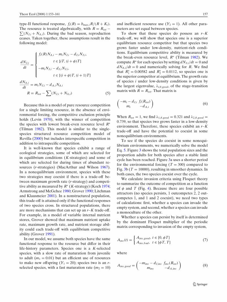
type-II functional response, fi(R) = bmax,i R/(R + Ki).The resource is treated algebraically, with R = Rtot −∑

(NJ,i + NA,i). During the bad season, reproductionceases. Taken together, these assumptions result in thefollowing model:

dNJ,i

dt=

⎧⎪⎪⎪⎪⎪⎨

⎪⎪⎪⎪⎪⎩

fi(R)NA,i − mi NJ,i − dJ,i NJ,i,

t ∈ [iT, (i + φ)T]−mi NJ,i − dJ,i NJ,i,

t ∈ [(i + φ)T, (i + 1)T]dNA,i

dt= mi NJ,i − dA,i NA,i

R = Rtot −∑

(NJ,i + NA,i) (5)

Because this is a model of pure resource competitionfor a single limiting resource, in the absence of envi-ronmental forcing, the competitive exclusion principleholds (Levin 1970), with the winner of competitionthe species with lowest break-even resource level R∗(Tilman 1982). This model is similar to the single-species structured resource competition model ofRevilla (2000) but includes interspecific competition inaddition to intraspecific competition.

It is well-known that species exhibit a range ofecological strategies, some of which are selected forin equilibrium conditions (K-strategies) and some ofwhich are selected for during times of abundant re-sources (r-strategies) (MacArthur and Wilson 1967).In a nonequilibrium environment, species with thesetwo strategies may coexist if there is a trade-off be-tween maximum growth rate (r-strategy) and competi-tive ability as measured by R∗ (K-strategy) (Koch 1974;Armstrong and McGehee 1980; Grover 1990; Litchmanand Klausmeier 2001). In a nonstructured population,this trade-off is attained only if the functional responsesof two species cross. In structured populations, thereare more mechanisms that can set up an r–K trade-off.For example, in a model of variable internal nutrientstores, Grover showed that maximum nutrient uptakerate, maximum growth rate, and nutrient storage abil-ity could each trade-off with equilibrium competitiveability (Grover 1991).

In our model, we assume both species have the samefunctional response to the resource but differ in theirlife-history parameters. Species one is a K-selectedspecies, with a slow rate of maturation from juvenileto adult (m1 = 0.01) but an efficient use of resourcesto make new offspring (Y1 = 20); species two is an r-selected species, with a fast maturation rate (m2 = 10)

and inefficient resource use (Y2 = 1). All other para-meters are set equal between species.

To show that these species do possess an r–Ktrade-off, we will show that species one is a superiorequilibrium resource competitor but that species twogrows faster under low-density, nutrient-rich condi-tions. Equilibrium competitive ability is measured bythe break-even resource level, R∗ (Tilman 1982). Wecompute R∗ for each species by setting dNJ,i/dt = 0 anddNA,i/dt = 0 and numerically solving for R. We findthat R∗

1 = 0.00582 and R∗2 = 0.0112, so species one is

the superior competitor at equilibrium. The growth rateof species i under low-density conditions is given bythe largest eigenvalue, λi,∅,good, of the stage-transitionmatrix with R = Rtot. That matrix is

(−mi − dJ,i fi(Rtot)

mi −dA,i

)(6)

When Rtot = 1, we find λ1,∅,good = 0.321 and λ2,∅,good =0.739, so that species two grows faster in a low-densityenvironment. Therefore, these species exhibit an r–Ktrade-off and have the potential to coexist in somenonequilibrium environments.

To see if the species do coexist in some nonequi-librium environments, we numerically solve the modelEq. 5. Figure 3 shows the total population sizes and theproportion adults for both species after a stable limitcycle has been reached. Figure 3a uses a shorter periodfor the environmental forcing (T = 300) compared toFig. 3b (T = 10000), resulting in smoother dynamics. Inboth cases, the two species coexist over the cycle.

We calculate invasion criteria using Floquet theoryto summarize the outcome of competition as a functionof φ and T (Fig. 4). Because there are four possibleattractors (no species persists, 1 outcompetes 2, 2 out-competes 1, and 1 and 2 coexist), we need two typesof calculations: first, whether a species can invade theempty system, and second, whether a species can invadea monoculture of the other.

Whether a species can persist by itself is determinedby the dominant Floquet multiplier of the periodicmatrix corresponding to invasion of the empty system,

Ainv(t) ={

Ainv,good, t ∈ [0, φT]Ainv,bad, t ∈ [φT, T] (7)

where

Ainv,good =(−minv − dJ,inv finv(Rtot)

minv −dA,inv

)(8)

158 Theor Ecol (2008) 1:153–161

a

b

Fig. 3 Asymptotic dynamics of competition between a K-selected (species 1, solid line) and an r-selected (species 2, dottedline) species in a seasonal environment. a φ = 0.6 and T = 300.b φ = 0.68 and T = 10000. Black bars denote the “bad” season

and

Ainv,bad =(−minv − dJ,inv 0

minv −dA,inv

)(9)

Because Ainv(t) is a piecewise-constant matrix, we cancompute the fundamental matrix X(t) using the matrixexponential (Gökçek 2004). The fundamental matrix is

X(t) = exp((1 − φ)T Ainv,bad) exp(φT Ainv,good), (10)

whose eigenvalues are the Floquet multipliers corre-sponding to invasion into the empty system and can be

Fig. 4 Outcome of competition between a K-selected (species 1)and an r-selected species (species 2) in a seasonal environmentwith period T and φ proportion “good” season, as determined byinvasion criteria using Floquet theory. Arrows on the top denotevalues for these boundaries when T → ∞ determined with a slowfluctuation approximation

easily calculated numerically (seeElectronic Appendix).When the dominant Floquet multiplier is greater thanone, max(Re(ρ)) > 1, the species can persist in mono-culture. The critical φ that allows growth for a givenT can be found numerically using Newton’s method(see Electronic Appendix). This approach gives the twoleftmost lines in Fig. 4.

To determine whether a species can invade a mono-culture of the other species, we first find the limit cyclesolution of the resident species alone then calculate theFloquet multipliers of the matrix corresponding to theinvader’s growth when rare. Here,

Agood,inv =(−minv − dJ,inv finv(Rres(t))

minv −dA,inv

)(11)

where “inv” denotes invader and “res” denotes residentand Rres(t) is determined from the monoculture limitcycle of the resident, which must be determined by nu-merically integrating a single-species version of Eq. 5.Abad,inv is the same as above. Again, the critical φ iswhere max(Re(ρ)) = 1, which gives the two right linesbounding the coexistence region in Fig. 4.

For large periods, population dynamics become step-like (Fig. 3b). Elsewhere, we have developed approxi-mate analytical techniques for studying competition inan alternating environment in this limit of slow fluc-tuations (Litchman and Klausmeier 2001; Klausmeierin preparation). That slow fluctuation approximationcan also be applied to this stage-structured model asfollows. Let λi,∅,good denote the dominant eigenvalueof the matrix corresponding to species i invading the

Theor Ecol (2008) 1:153–161 159

empty system in the good season, λi,{ j},good denote thedominant eigenvalue of the matrix corresponding tospecies i invading species j at equilibrium in the goodseason, and λi,∅,bad denote the dominant eigenvalue ofthe matrix corresponding to species i declining in thebad season. The critical φ for persistence of species i byitself is

φ = λi,∅,bad

λi,∅,bad − λi,∅,good(12)

and the critical φ for invasion of species i into a mono-culture of species j is

φ =(λi,∅,badλ j,∅,good − λi,∅,goodλ j,∅,bad+λi,{ j},goodλ j,∅,bad

)

/(λi,∅,badλ j,∅,good−λi,{ j},goodλ j,∅,good−λi,∅,goodλ j,∅,bad

+ λi,{ j},goodλ j,∅,bad

)(13)

(Klausmeier in preparation). For the parameters usedhere, the critical φ values for persistence in monocul-ture are φ1 = 0.2373 and φ2 = 0.1192, and the critical φ

values for coexistence are φ1 = 0.6231 and φ2 = 0.7606(see Electronic Appendix). These values are noted witharrows in Fig. 4, where they can be seen to agree withthe numerical results generated with Floquet theory asthe period T → ∞.

This example shows that coexistence of an r- and aK-selected species is possible if there is a life-history-mediated trade-off between maximum growth rate andcompetitive ability, even if both species share the samefunctional response. Unlike the nonstructured pop-ulation model we previously studied (Litchman andKlausmeier 2001), there is no switch in competitivedominance for small periods. Instead, the K-selectedspecies dominates for all φ for small T. There is also asmall region of parameter space where founder controloccurs (Fig. 4).

Example 3: Stability of a limit cycle

The most common use of Floquet theory is to testthe stability of a limit cycle solution. This is usefulin understanding how dynamics depend on parametervalues. Here, we illustrate this use on a classic modelof a three-species food chain that is known to havelimit cycle solutions that can become unstable as modelparameters are changed (Hastings and Powell 1991;Kuznetsov and Rinaldi 1996).

The Hastings–Powell food chain model consists ofthree species (basal x, intermediate predator y, andtop predator z). The basal species grows logistically,every resource–consumer pair is coupled by a type-

II functional response, and the intermediate and toppredators experience density-independent mortality(Hastings and Powell 1991). The resultant nondimen-sionalized model is

dxdt

= x(1 − x) − a1x1 + b1x

y = f1 (14)

dydt

= a1x1 + b1x

y − a2 y1 + b2 y

z − d1 y = f2 (15)

dzdt

= a2 y1 + b2 y

z − d2z = f3 (16)

(Hastings and Powell 1991).Following Hastings and Powell (1991), we focus on

the nondimensional parameter b1. Using brute forcenumerical solution of the model, Hastings and Powellshowed that, as b1 increased from 2.25 to 2.4, the modelundergoes the period-doubling route to chaos (Fig. 4cin Hastings and Powell 1991, our Fig. 5a, b). Here,we investigate the first period doubling using Floquettheory.

Before we can study the stability of the limit cyclesolution, first we have to locate it, which we must donumerically. We must locate one point on the limit

a

c

b

Fig. 5 Stability of a limit cycle solution in the Hastings andPowell (1991) food chain model. Parameters are: a1 = 5.0, a2 =0.1, b 2 = 2.0, d1 = 0.4, and d2 = 0.01. a–b Dynamics of y. a Alimit cycle with b1 = 2.28. b A period-doubled limit cycle withb 1 = 2.3. c Dominant Floquet multiplier of the limit cycle as afunction of b1. Around b1 = 2.291, there is a period-doublingbifurcation

160 Theor Ecol (2008) 1:153–161

cycle, as well as its period T, such that x(t + T) = x(t),y(t + T) = y(t), and z(t + T) = z(t). We do this usingNewton’s method through Mathematica’s FindRootcommand (see Electronic Appendix).

Once the limit cycle is in hand, we test its stabilityby asking if small perturbations away from the limitcycle grow or shrink over a complete period. This cor-responds to finding the stability of the periodic systemobtained by linearizing the full model Eq. 10 aroundthe limit cycle (Grimshaw 1993). Define the Jacobianmatrix of Eq. 10 as

J(t) =

⎛

⎜⎜⎜⎜⎜⎜⎝

∂ f1

∂x∂ f1

∂y∂ f1

∂z∂ f2

∂x∂ f2

∂y∂ f2

∂z∂ f3

∂x∂ f3

∂y∂ f3

∂z

⎞

⎟⎟⎟⎟⎟⎟⎠

(x(t),y(t),z(t))limit cycle

(17)

The Floquet multipliers of J(t) determine the stabilityof the limit cycle. Figure 5c shows that the dominantFloquet multiplier of J(t) as b1 is increased from 2.28 to2.32. Near b1 = 2.291, the dominant Floquet multiplierpasses through −1, signifying a period-doubling bifur-cation of the limit cycle. This corroborates the bruteforce numerical analysis of Hastings and Powell (1991).

Discussion

The three examples in this paper demonstrate thatFloquet theory is a versatile tool for studying the ecol-ogy and evolution of periodic systems. Floquet theorydefines fitness in periodic environments, can calculateinvasion criteria for competing species, and can be usedto test the stability of limit cycle solutions. Given thesediverse uses and the ubiquity of both structured popu-lations and periodic systems in nature, Floquet theoryshould be a useful addition to theoreticians’ toolboxes.Although Floquet theory is a linear theory, nonlinearmodels can be linearized near limit cycle solutions toenable the use of Floquet theory.

An alternative way to compute Floquet exponentsand multipliers is to use numerical continuation soft-ware such as AUTO (Doedel et al. 2001), XPPAUT(Ermentrout 2002), CONTENT (Kuznetsov andLevitin 1996), or MATCONT (Dhooge et al. 2003).These programs provide powerful environments foranalyzing the behavior of nonlinear dynamical systems.See van Coller (1997) for an ecological introduction tocontinuation software.

Floquet theory deals with continuous-time systems.The theory of periodic discrete-time systems is closelyanalogous (Caswell 2001, chapter 13). In that case,

one can multiply the T transition matrices together todetermine how a perturbation changes over a period,which is similar to finding the fundamental matrix.

One limitation of Floquet theory is that it appliesonly to periodic systems. Although many systems ex-perience periodic forcing, others experience stochasticor chaotic forcing. In these cases, the more generalLyapunov exponents described by Metz et al. (1992)play the role of Floquet exponents (see also Ferriereand Gatto 1995). Conceptually similar to Floquet ex-ponents (and therefore to eigenvalues of the Jacobianmatrix associated with an equilibrium point), Lyapunovexponents are more challenging to compute numeri-cally because, instead of calculating how a perturbationgrows or shrinks over one period, this must be done inthe limit at T → ∞. For a practical algorithm for this incontinuous systems, see Wolf et al. (1985).

Acknowledgements I thank Chad Brassil, Jeremy Fox, HalSmith, and Robin Snyder for useful discussion and comments onthis manuscript. This research was supported by NSF grant DEB-0610532, a grant from the James S. McDonnell Foundation, andthe NCEAS working group “Evolving Metacommunities.” Thisis publication number 1461 of the Kellogg Biological Station.

References

Armstrong RA, McGehee R (1980) Competitive exclusion. AmNat 115:151–170

Brassil CE (2006) Can environmental variation generate positiveindirect effects in a model of shared predation? Am Nat167:43–54

Caswell H (2001) Matrix population models: construction, analy-sis, and interpretation, 2nd edn. Sinauer, Sunderland

Chesson P (1994) Multispecies competition in variable environ-ments. Theor Popul Biol 45:227–276

DeAngelis DL, Waterhouse JC (1987) Equilibrium and nonequi-librium conepts in ecological models. Ecol Monogr 57:1–21

Dhooge A, Govaerts W, Kuznetsov YuA (2003) MatCont: aMATLAB package for numerical bifurcation analysis ofODEs. ACM Trans Math Softw 29:141–164

Doedel EJ, Paffenroth RC, Champneys AR, Fairgrieve TF,Kuznetsov YuA, Oldeman BE, Sandstede B, Wang XJ(2001) AUTO2000: continuation and bifurcation softwarefor ordinary differential equations. https://sourceforge.net/projects/auto2000/

Drazin PG (1992) Nonlinear systems. Cambridge UniversityPress, Cambridge

Ermentrout B (2002) Simulating, analyzing, and animating dy-namical systems: a guide to XPPAUT for researchers andstudents. SIAM, Philadelphia.

Ferriere R, Gatto M (1995) Lyapunov exponents and the math-ematics of invasion in oscillatory or chaotic populations.Theor Popul Biol 48:126–171

Gonzalez A, Holt RD (2002) The inflationary effects of environ-mental fluctuations in source-sink systems. Proc Natl AcadSci U S A 99:14872–14877

Gökçek C (2004) Stability analysis of periodically switched linearsystems using Floquet theory. Math Probl Eng 2004:1–10

Theor Ecol (2008) 1:153–161 161

Grimshaw R (1993) Nonlinear ordinary differential equations.CRC, Ann Arbor

Grover JP (1990) Resource competition in a variable environ-ment: phytoplankton growing according to Monod’s model.Am Nat 136:771–789

Grover JP (1991) Resource competition in a variable environ-ment: phytoplankton growing according to the variable-internal-stores model. Am Nat 138:811–835

Grover JP, Holt RD (1998) Disentangling resource and apparentcompetition: realistic models for plant-herbivore communi-ties. J Theor Biol 191:353–376

Hastings A (1997) Population biology: concepts and models.Springer, Berlin Heidelberg New York

Hastings A, Powell T (1991) Chaos in a three-species food chain.Ecology 72:896–903

Holt RD, Barfield M, Gonzalez A (2003) Impacts of envi-ronmental variability in open populations and communi-ties: “inflation” in sink environments. Theor Popul Biol 64:315–330

Kaitala V, Lundberg P, Ripa J, Ylikarjula J (1997) Red blueand green: dyeing population dynamics. Ann Zool Fenn 34:217–228

Koch AL (1974) Competition coexistence of two predators utiliz-ing the same prey under constant environmental conditions.J Theor Biol 44:387–395

Kooi BW, Troost TA (2006) Advantage of storage in a fluctuatingenvironment. Theor Popul Biol 70:527–541

Kratz TK, Deegan LA, Harmon ME, Lauenroth WK (2003)Ecological variability in space and time: insights gained fromthe US LTER program. BioScience 53:57–67

Kuznetsov YuA, Levitin VV (1996) CONTENT: a multi-platform environment for analyzing dynamical systems.Dynamical Systems Laboratory, Centrum voor Wiskundeen Informatica, Amsterdam. http://www.math.uu.nl/people/kuznet/CONTENT/

Kuznetsov YuA, Rinaldi S (1996) Remarks on food chain dy-namics. Math Biosci 134:1–33

Levin SA (1970) Community equilibria and stability, and anextension of the competitive exclusion principle. Am Nat104:413–423

Litchman E, Klausmeier CA (2001) Competition of phytoplank-ton under fluctuating light. Am Nat 157:170–187

MacArthur RH, Wilson EO (1967) The theory of island biogeog-raphy. Princeton University Press, Princeton

May RM (1974) Stability and complexity in model ecosystems,2nd edn. Princeton University Press, Princeton

Metz JAJ, Diekmann O (eds) (1986) The dynamics of physio-logically structured populations. Springer, Berlin HeidelbergNew York

Metz JAJ, Nisbet RM, Geritz SAH (1992) How should wedefine “fitness” for general ecological scenarios? TrendsEcol Evol 7:198–202

Mylius SD, Diekmann O (2001) The resident strikes back:invader-induced switching of resident attractor. J Theor Biol211:297–311

Namba T, Takahashi S (1993) Competitive coexistence in a sea-sonally fluctuating environment. II. Multiple stable statesand invasion success. Theor Popul Biol 44:374–402

Nisbet RM, Gurney WSC (1982) Modelling fluctuating popula-tions. Wiley, New York

Revilla TA (2000) Resource competition in stage-structuredpopulations. J Theor Biol 204:289–298

Roy M, Holt RD, Barfield M (2005) Temporal autocorrela-tion can enhance the persistence and abundance of meta-populations comprised of coupled sinks. Am Nat 166:246–261

Steele JH, Henderson EW (1984) Modeling long-term fluctua-tions in fish stocks. Science 224:985–987

Strogatz SH (1994) Nonlinear dynamics and chaos. Westview,Cambridge

Thoreau HD (1854) Walden; or, life in the woods. Penguin,New York

Tilman D (1982) Resource competition and community struc-ture. Princeton University Press, Princeton

Tilman D, Kareiva P (eds) (1997) Spatial ecology: the role ofspace in population dynamics and interspecific interactions.Princeton University Press, Princeton.

van Coller, L (1997) Automated techniques for the qualitativeanalysis of ecological models: continuous models. ConservEcol 1:5. http://www.consecol.org/vol1/iss1/art5/

Wolf A, Swift JB, Swinney HL, Vastano JA (1985) Determin-ing Lyapunov exponents from a time series. Physica D 16:285–317

Wolfram Research, Inc. (2007) Mathematica, version 6.0.Wolfram, Champaign

Yodzis P (1989) Introduction to theoretical ecology. Harper andRow, New York