Floods and droughts

Definitions

Flood: Floods occur when a drainage basin experiences an unusually intense or prolonged water input. Flood is usually viewed as an event in which the streamflowexceeds the channel capacity, resulting on overland flow (the floodplain is inundated), but the terms is also often applied more generally to unusually high discharge events.

Drought: A drought is an extended period (months, years) that a region experiences a deficiency in water supply, generally because of reduced precipitation.

http://www.11terra.com/rising_seas

http://library.thinkquest.org/03oct/00477/NatDisasterPages/Heidi%20Draught/drought/droughtclassification.htm.htm

Floodplain

A floodplain is nearly flat land adjacent to a mature stream or river extending from the stream channel to the base of the enclosing valley. As the name implies, floodplains are water covered during floods. Of course not all streams and rivers have floodplains.

Floodplains are fertile land for agriculture (sediments are deposited by floods) and they can support rich ecosystems. They are not particularly smart places for human settlements.

Flood frequency analysis

http://www.ceh.ac.uk/data/nrfa/data/timeseries_plots.html

Goal: Using a given record of stream flows, such as a left, find the exceedence probability and return period of discharge events of a given size. Flood frequency analysis useful for developing floodplain management strategies and informing infrastructure design.

Getting exceedence probabilityExceedence probability EP(Q) is the probability of discharge Q exceeding a

specified value of discharge Qsp

EP(Q) = Probability {Q > Qsp} = 1 – F(Q)

Where F(Q) is the cumulative distribution function (CDF) of discharge:

F(Q) = Probability {Q ≤ Qsp}

http://www.itl.nist.gov/div898/handbook/eda/section3/eda362.htm

Below: Probability density function (PDF) and cumulative distribution function (CDF) for a normal distribution

Return periodIf EP(Q) stays constant with time, then the interval between occurrences of the event Q > Qsp is 1/EP(Q). Thus exceedance probability can be expressed in terms of a return period TR(Q), also know as a recurrence interval.

TR(Q) = 1/EP(Q) = 1/(1-F(Q))

If we consider the statistics using the largest discharge for each year (as is typically done), then TR(Q) is the average number of years between intervals when Q > Qsp.

Hence, by definition, the 100 year flood is the annual peak discharge with an event probability of 0.01:

TR(Q) = 1/EP(Q) TR(Q) = 1/0.01 = 100 years

Z-score transformation

http://www.thefullwiki.org/Z_scores

Assume for the moment that the largest discharge events for each year are drawn from a normal distribution hence having the characteristics depicted in the figure below. For each discharge value, we can compute a Z-score:

Z = [Q - <Q>]/SD

Where <Q> is the average of all of the largest annual discharge values, Q is the largest discharge for a given year, and SD is the standard deviation of <Q>.

As seen in the figure:

For Q = <Q>, Z=0, EP(Q)=50%For Q = <Q> + SD, Z=1, EP(Q) =16%For Q = <Q> + 2.SD, Z=2, EP(Q) = 2.3%For Q = <Q> + 3.SD, Z=3, EP(Q) = 0.01%

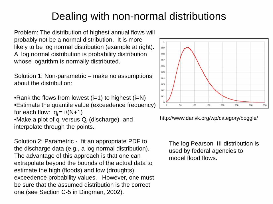
Dealing with non-normal distributionsProblem: The distribution of highest annual flows will probably not be a normal distribution. It is more likely to be log normal distribution (example at right). A log normal distribution is probability distribution whose logarithm is normally distributed.

Solution 1: Non-parametric – make no assumptions about the distribution:

•Rank the flows from lowest (i=1) to highest (i=N)•Estimate the quantile value (exceedence frequency) for each flow: qi = i/(N+1)•Make a plot of qi versus Qi (discharge) and interpolate through the points.

Solution 2: Parametric - fit an appropriate PDF to the discharge data (e.g., a log normal distribution). The advantage of this approach is that one can extrapolate beyond the bounds of the actual data to estimate the high (floods) and low (droughts) exceedence probability values. However, one must be sure that the assumed distribution is the correct one (see Section C-5 in Dingman, 2002).

http://www.danvk.org/wp/category/boggle/

The log Pearson III distribution is used by federal agencies to model flood flows.

Flow frequency curve

http://pubs.usgs.gov/wri/wri974073/report.html

At right is the flow frequency curve for the Virgin River at Littlefield AZ (gauging station 09415000) based on different estimates. The 100 year flood (annual exceedenceprobability of 1%) is about 750 m3s-1. Half of the time (exceedence probability of 50%) , the discharge exceeds about 150 m3s-1

Source: USGS

Front Range Colorado: Mixed Population Floods

In the Front Range, the largest floods are due to rain events, though snowmelt floods are more common

In the Alpine, rain storms are not large enough to create significant floods, and the hydrology is dominated by snowmelt

Predicting flow at un-gauged sites

The techniques just discussed apply to gauged streams. However, we may want to get exceedence probability relations for ungauged streams:

•Get magnitude exceedence probability relations at gauging stations from the surrounding area.

•Use multiple linear regression to relate the magnitude of floods with specified exceedence probabilities at those gauging stations to characteristics of their drainage basins (e.g., area, slope, location, forest cover, elevation, geology, channel size).

•Apply the equation to the ungauged stream based on the characteristics of its drainage

Regional equations for predicting flood peaks

Source: USGS

Floodplain management

Flood control dams: These reduce the peak flood discharge associated with a given exceedence probability at locations downstream of the dam. Their effects decrease rapidly with downstream distance and tend to be less effective for larger floods.

Dikes and levees: Designed to prevent flooding behind them. They can increase flood levels downstream. Overtopping of dikes and levees can have catastrophic consequences (e.g., New Orleans after Hurricane Katrina, see photograph at bottom right)

http://www.uwsp.edu/geO/faculty/ozsvath/images/flood_control_dam.htm

http://www.hurricanekatrina.com/

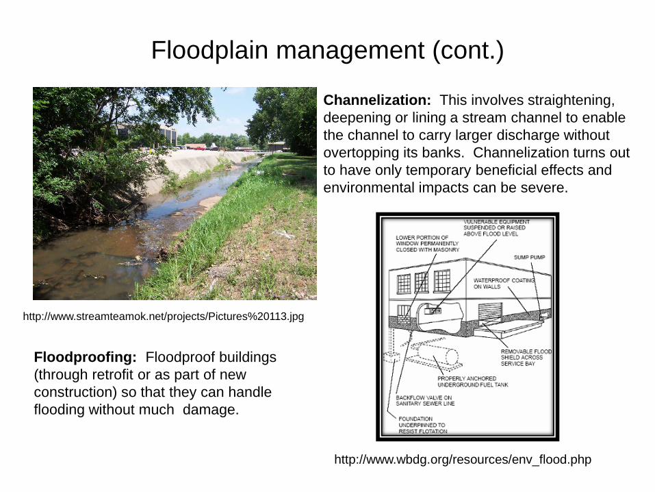
Floodplain management (cont.)

Channelization: This involves straightening, deepening or lining a stream channel to enable the channel to carry larger discharge without overtopping its banks. Channelization turns out to have only temporary beneficial effects and environmental impacts can be severe.

http://www.streamteamok.net/projects/Pictures%20113.jpg

Floodproofing: Floodproof buildings (through retrofit or as part of new construction) so that they can handle flooding without much damage.

http://www.wbdg.org/resources/env_flood.php

Floodplain management (cont.)

Removal of structures: Remove buildings in harm’s way

Flood warning: Provide enough advance warning of a flood (e.g., with a siren, as in Boulder) for people to get out of the area anticipated to be affected. Flood warming works best on large rivers that respond relatively slowly an predictably of water input events. Warning systems are less effective when it comes to flash floods that require rapid response time (e.g., Big Thompson River 1976, , we’ll look at this shortly).

Floodplain zoning: Land use controls that limit development on flood prone areas

http://www.rcscomm.net/floodwarning.html

http://www.co.washington.wi.us/departments.iml?Detail=147

Boulder Creek, 1894Bridge at 4th St.

Denver Public Library

Near 7th St., looking east

Between May 30-June 1, heavy rains fell in the Boulder and South Boulder Creek basins. Rainfall records for a 96-hour period showed that the mountain drainage area received from 4.5 to 6 inches of precipitation which combined with snowmelt runoff. The estimated flow on Boulder Creek at 4th Street was 11,000 to 13,500 cfs, similar to the flow of a 100-year flood of 12,000 cfs (from US Army Corps of Engineers).

http://www.boulderfloods.org/Mapviewer/boulder_centrall_floodhazardzone.htm

South Boulder Creek, 1938Closeup of Dance Hall.

Both Denver Public Library

Houses on the brink

The storm produced general rains over all of eastern Colorado, with over 6 inches reported west of Eldorado Springs. Boulder reported 3.62 inches of precipitation from 31 August to 4 September with 2.32 inches falling during 2 September. Eldorado Springs had 4.42 inches of rainfall. Approximately 80 % of the total precipitation falling in the South Boulder Creek basin fell in the late afternoon and evening of 2 September. The resulting flood, with a peak discharge of 7390 cfsarrived at Eldorado Springs at 10 PM on 2 September.

http://bcn.boulder.co.us/basin/history/1938flood.html

Big Thomson River, 1976

Denver Post, David Buresh

Denver Post, Dave Cupp

The flood was set off by a severe rainstorm (convection with easterly flow) that stalled between Estes Park and Loveland on July 31, 1976. The storm dumped nearly 8 inches of rain in one hour, and up to 12 inches of rain in four hours . The flood claimed 144 lives and destroyed more than 400 homes. The peak flood flow on the Big Thompson was computed to be just over 30,000 cfs. A 100 year flood? 1000 year? 10,000 year? There is debate.

Source: USGS

Source: USGS

Water Resources Research

Bijou Creek

Big Thompson

Source: O’Connor and Costa

Source: O’Connor and Costa

Source: O’Connor and Costa

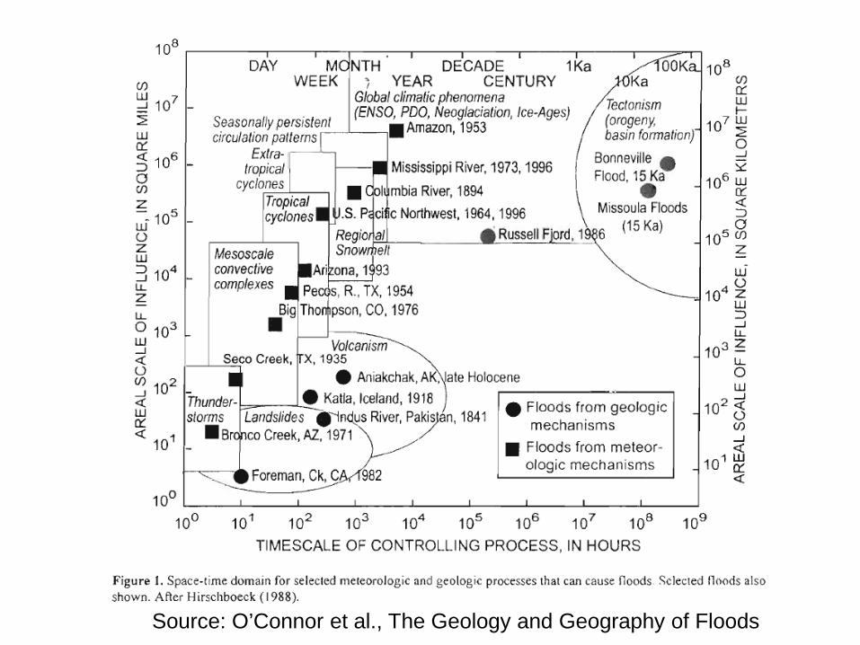
Source: O’Connor et al., The Geology and Geography of Floods

Source: O’Connor et al., The Geology and Geography of Floods

The Missoula Floods – a glacial outburst : One of the largest floods known in geologic record

http://www.nwcreation.net/articles/missoulaflood.htm

Lake Bonneville flood, 15,000 BPhttp://imnh.isu.edu/digitalatlas/hydr/lkbflood/lbf.htmLake Bonneville was the precursor of the Great Salt Lake

and once covered an area of more than 19,000 square miles. Approximately 15,000 years ago, the lake suddenly discharged to the north. This flood is thought to be caused by capture of the Bear River which greatly increased the supply of water to the Bonneville Basin. The flood waters flowed over Red Rock Pass (where the failure occurred) in southeastern Idaho and continued westward, following the approximate path of the present Snake River. Peak flow may have been 15 million cfs. The Melon Gravels deposited by the flood average three feet in diameter, but some well-rounded boulders range up to 10 feet in diameter. Boulders were dumped in unsorted deposits up to 300 feet thick.(http://imnh.isu.edu/digitalatlas/hydr/lkbflood/lbf.htm)

http://travellogs.us/Miscellaneous/Geology/Melon%20Rocks/Melon%20Rocks.htm

The Laurentide Ice Sheet and the routing of overflow from the Lake Aggasiz basin (dashed line) to the Gulf of Mexico just before the Younger Dryas (a) and routing of overflow from Lake Aggasizthrough the Great Lakes to the St. Lawrence and northern North Atlantic during the Younger Dryas(b) [from Broecker et al., 1989, by permission of Nature]. Massive discharge of freshwater into the North Atlantic from the melting Laurentide Ice Sheet could have disrupted the ocean thermohalinecirculation, initiating the YD cold event.

The Younger Dryas, 11,500 BP, initiated by a massive flood?

Open channel flow and flood wavesStream discharge Q can be expressed as follows:

Q = U.Y.B (Eq. 1)

Where U is the average flow velocity (m s-1), Y is the average depth of the flow (m) and B is the water surface width (m).

Open channel velocity U can be given by the Manning Equation :

U = (um.Y2/3.S1/2)/n (Eq. 2)

S is the water surface slope, Manning’s “n” is a factor characterizing channel conductance/resistance (it depends on channel roughness and irregularity) and um is a unit conversion factor.

Dignman (1984) has shown that the velocity of a flood wave UF is:

UF = 1/B.∂Q/∂Y (Eq. 3)

Where B is the water surface width (channel width), Q is the discharge, and Y is the average depth of the flow.

Open channel flow and flood waves (cont.)Q = U.Y.B (Eq. 1)U = (um.Y2/3.S1/2)/n (Eq. 2)

Rearrange and combine the above two equations:

U = Q/(Y.B) U = (um.Y2/3.S1/2)/n

Q/(Y.B) = (um.Y2/3.S1/2)/nQ = Y3/3.B.(um.Y2/3.S1/2)/n

Q = B.(um.Y5/3.S1/2)/n (Eq. 4)

Differentiate with respect to Y

∂Q/ ∂Q = 5/3.(um.Y2/3.S1/2.B)/n (Eq. 5)

Substitute the Manning Equation (Eq. 2) and Eq. 4 into the equation for flood wave velocity (Eq. 3) and we get

UF = 5/3.U

Meaning that the flood wave moves faster (1.67 times) the the water itself!

Dingman 2002, Figure 9-2

Open channel flow and flood waves (cont.)

Q = B.(um.Y5/3.S1/2)/n

UF = 5/3.U

These two equation work for flood waves that remain within the river channel. The relationship between flow velocity and flood wave velocity may be altered of the stream overtops the channel banks and inundates the flood plain.

Dingman 2002, Figure 9-2

Velocities tend to be lower in the overbank portion of the flood because they the water is shallower and encounters higher resistance due to vegetation (e.g., trees get in the way). The flood wave velocity equation can be adjusted to account for such effects.

http://www.geograph.org.uk/photo/148021

Example: Glen Canyon Dam release

http://www.glencanyon.org/library/bureauhistory.php

In April 2009 there was a large water release from the Glen Canyon Dam on the Colorado River, intended to improve stream habitat by mimicking the spring discharge peak that would have naturally occurred without the dam in place.

Consider the travel time of the flood wave associated with the release from Lee’s Ferry (in Glen Canyon) to the Grand Canyon.

http://www.grandcanyonairlines.com/gca/gcaimg/fulls/glencanyon4.jpg

Glen Canyon example (cont.)

Peak discharge Q at Lee’s Ferry: about 12,000 cfs at 2200h, 4/18/09

Peak discharge Q at Grand Canyon: was about 12,500 cfs at 1600h, 4/19/09

Travel time of flood wave = 18 hours = 64,800 s

Distance travelled = 87 miles = 459,360 feet

UF = 459,360 ft/64,800 sec ≈ 7 ft s-1

U = 2.5 feet s-1

Hence UF ≈ 2.7.U

Question: Why higher than 1.67?Primary answer: Channel morphology

Channel width at Lee’s Ferry: 415 ftChannel width at Grand Canyon: 290 ft

http://www.sangres.com/dimages/arizona/coconino-county/Glen-Canyon-Dam.gif

Glen Canyon example (cont.)

Go back to the equation for flood wave velocity from Dingman(1984):

UF = 1/B.∂Q/∂Y (Eq. 3)

Where B is the water surface width (channel width), Q is the discharge, and Y is the average depth of the flow. Hence, because the channel narrows, the flood wave propagates faster than predicted.

290 ft/415 ft = 70%, i.e., Grand Canyon channel width is 70% of the channel width at Lee’s Ferry

70% of 2.7 =1.9, closer to 1.67 but still high.

Explanation: Water velocity increases slightly downstream.

Drought

Drought is part of natural climate variability. There are three basic sequences of drought and associated impacts:

Meteorological drought: Deficit in precipitation, often (not always) accompanied by above average temperatures, high winds, low humidity and high solar radiation.

Agricultural drought: Continued precipitation deficit, leading to a soil water deficit, hindering agriculture and natural plant growth.

Hydrologic drought: The precipitation deficit continues, and stream discharge, lake wetland and reservoir levels drop, with impacts on wildlife habitat.

http://www.drought.unl.edu/whatis/concept.htm

Low flow analysis: Flow duration curve

http://streamflow.engr.oregonstate.edu/analysis/flow/tutorial.htm

The flow duration curve is a useful tool for streamflow analysis; it gives the flow associated with any exceedence or non-exceedenceprobability. The flow which is exceeded 95% of the time is an index of water availability used for design purposes. In the example at right, for the Alsea River at Tidewater (WY), the 95% exceedence flow is about 80 cfs. Flow duration curves are computed using daily streamflow data.

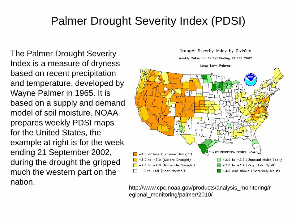
Palmer Drought Severity Index (PDSI)

http://www.cpc.noaa.gov/products/analysis_monitoring/regional_monitoring/palmer/2010/

The Palmer Drought Severity Index is a measure of dryness based on recent precipitation and temperature, developed by Wayne Palmer in 1965. It is based on a supply and demand model of soil moisture. NOAA prepares weekly PDSI maps for the United States, the example at right is for the week ending 21 September 2002, during the drought the gripped much the western part on the nation.

Calculating PDSI

“Computation of PDSI begins with the determination of monthly departure of moisture from normal by estimating the gaps between actual precipitation and precipitation that is climatically appropriate for existing conditions (CAFEC-P).

The CAFEC-P can be obtained from the basic terms of the water balance equation, which deducts the expected supply from the expected demand factors to get the water demand that must be met by precipitation.

Parameters of the CAFEC include evapotranspiration, soil recharge, runoff, and moisture loss from the surface layer. The monthly moisture anomalies are then converted into the indices of moisture anomaly by multiplying by a weighting factor.

Finally, dryness or wetness severity is deduced from the moisture anomaly index and the PDSI of the previous month. Theoretically, PDSI is a standardized measure, ranging from about −6.0 to +6.0”

From: Spatial Variation and Trends in PDSI and SPI Indices and Their Relation to Streamflow in 10 Large Regions of China, Jianqing Zhai, Journal of Climate, 23, 649-663.

Palmer Drought Severity Index (cont.)

PDSI for July 1934, during the “Dust Bowl”

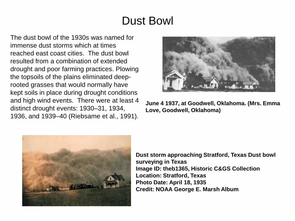
Dust BowlThe dust bowl of the 1930s was named for immense dust storms which at times reached east coast cities. The dust bowl resulted from a combination of extended drought and poor farming practices. Plowing the topsoils of the plains eliminated deep-rooted grasses that would normally have kept soils in place during drought conditions and high wind events. There were at least 4 distinct drought events: 1930–31, 1934, 1936, and 1939–40 (Riebsame et al., 1991).

Dust storm approaching Stratford, Texas Dust bowl surveying in Texas Image ID: theb1365, Historic C&GS Collection Location: Stratford, Texas Photo Date: April 18, 1935 Credit: NOAA George E. Marsh Album

June 4 1937, at Goodwell, Oklahoma. (Mrs. Emma Love, Goodwell, Oklahoma)

M Hoerling, A Kumar Science 2003;299:691-694

Temperature and precipitation anomalies, 1998-2002While Western U.S. drought was extreme in 2002, it was preceded by prolonged below-normal precipitation and above-normal temperatures during 1998–2002 over an extensive swath of the Northern Hemisphere mid-latitudes spanning the United States, the Mediterranean, southern Europe, and Southwest and Central Asia

The figure above shows observed, standardized 4-year–averaged SST anomalies for June 1998 through May 2002 (top), and monthly anomalies for the climatological warm pool region of the tropical Indian and west Pacific (left) and the climatological cold tongue region of the equatorial east Pacific (right)

M Hoerling, A Kumar Science 2003;299:691-694

A n unusual pattern of sea surface temperatures

Global climate models (GCMs) driven by the observed monthly varying anomalies in sea surface temperature were able to reproduce the basic pattern of annual averaged surface temperature (left) and precipitation (right) anomalies observed over the 4-year period June 1998–May 2002. Conclusion: the drought was largely driven by ocean conditions.

M Hoerling, A Kumar Science 2003;299:691-694

Modeling temperature and precipitation anomalies

The observed pressure height anomaly field at the 200 hPa level over the 4-year period June 1998–May 2002 (left) shows an almost uninterrupted zonal belt of unusually high pressure spanning the middle latitudes. The anomaly field as simulated by atmospheric GCMs forced with the observed, monthly varying SST and sea ice anomalies of the period is similar. Drying of the lower atmosphere is consistent with this pattern.

M Hoerling, A Kumar Science 2003;299:691-694

Atmospheric circulation anomalies

Drought feedback processes

Drought can be exacerbated by feedback processes. The figure at right conceptualizes processes in the Sahel of Africa. If the land dries out, there will be less vegetation, meaning less evaporation from the land, and more solar radiation will be reflected from the surface These processes weaken the monsoon that brings rainfall to the area. The feedback can involve land degradation due to human activities.

http://oceanworld.tamu.edu/resources/environment-book/desertificationinsahel.html , from Dryland Systems in Ecosystems and Human Well-Being: Current State and Trends

Rain follows the plow?“Rain follows the plow” refers to a late 19th century theory of climatology, popular in the American West and Australia. It finds it origin with Charles Dana Wilber, a land speculator, journalist, author and champion of the American West as a site of agricultural development. From his 1881 book The Great Valleys and Prairies of Nebraska and the Northwest:

"Suppose (an army of frontier farmers) 50 miles, in width, from Manitoba to Texas, could acting in concert, turn over the prairie sod, and after deep plowing and receiving the rain and moisture, present a new surface of green growing crops instead of dry, hard baked earth covered with sparse buffalo grass. No one can question or doubt the inevitable effect of this cooling condensing surface upon the moisture in the atmosphere as it moves over by the Western winds. A reduction of temperature must at once occur, accompanied by the usual phenomena of showers. The chief agency in this transformation is agriculture. To be more concise. Rain follows the plow."

http://homesteadcongress.blogspot.com/2009/10/homestead-myth-rain-follows-plow.html

http://science.discovery.com/top-ten/2009/science-mistakes/science-mistakes-07.html

Rain follows the plow?The basis of the theory is that agriculture would affect the climate of these semi-arid and arid lands, increasing rainfall and hence making them lush and productive. The theory was promoted as a justification for the settlement of the “Great American Desert” (the Great Plains). It was also used to justify the expansion of wheat growing in marginal lands in Australia.

Today, we would view the argument in terms of precipitation recycling (discussed earlier in the semester). Precipitation recycling is the fraction of precipitation that falls within a watershed (or region) due to water that is evapotranspirated from that region and then falls back within the same region.

http://www.physicalgeography.net/fundamentals/7t.html http://severe-wx.pbworks.com/w/page/15957990/Thunderstorms

Rain follows the plow?

F+

F+

PL/P = 1/(1+ 2.F+/ET.A)

P = Total precipitationPL = Precipitation of local originET = EvapotranspirationA = Area of watershedF+ = Vertically integrated vapor flux directed into the watershed (advectivemoisture term)

ET

From the formulation of Brubaker et al. (2003):

To get a high recycling ratio (P/PL)you want a large ET rateand a small advective moisture term.

P

Dingman 2002 Figure 2-3

http://www.bopmyspace.com/image_50/thunderstorm

Rain follows the plow?

The problem: For most regions, including the American west, the bulk of precipitation is “imported” in that the water vapor associated with the precipitation comes from outside of the region.

http://memory.loc.gov/award/nbhips/lca/107/10785r.jpg

Hence:

Plow the fields and plant crops. Transpiration and bare soil evaporation take soil moisture and put it into the atmosphere as water vapor. While some of the water vapor may fall back as rain within the same general region, most is carried away downstream.

Rain does not follow the plow. The plow needs to follow the rain.