floodriskassessment dufrain bd 1 of 30 1 of 30 ... to carry out the analysis and build a model. ......
TRANSCRIPT
FloodRiskAssessment_DuFrain_BD 1 of 30 Develop by NSF Grant iGETT
Lu_Student_Guide_Flood Risk
• Name: Barbara DuFrain • Institution: Del Mar College • Email: [email protected] • Phone: 361 698-1299 • Title : Flood Risk Assessment – Disaster Management
Using Remote Sensing and Landsat data for Flood Risk Assessment
Corpus Christi has had extensive expansion to the South West. Canals have been cut into the Oso creek and into the banks of Oso bay. How does Land cover and physical properties of the land affect the amount of run-off? Many locations are at risk for Flooding. This LU uses real world data and methods to create and test analytical models to identify flood risk in the Oso Creek-Nueces-Rio Grand-Coastal Basin. The students will use the LandSat images to identifying the area and acreage of Land Use Change (LUC). The flood risk will use the slope, aspect, land use, precipitation, and run off and other possible factors. Students function as operational teams during the project. During the LU each team is directed to the appropriate RS data and GIS data to capture and massage data for analysis. The teams are provided the instructions and procedures to carry out the analysis and build a model. The students use the RS and GIS data to assess the risk of floods for different Land Use and Land Cover (LULC).
– The LU is comprised of six Lab and Exercise sections. – Part 1. RS Introduction & ENVI Tutorial for Corpus Christi
Students are provided with Step by Step instructions. – Part 2. ENVI Tutorial for Corpus Christi Using Landsat Data.
Ann Johnson, March 2008. – Part 3. Student Teams perform PCA Change Analysis for the selected
Landsat temporal data. – Part 4. Student Teams collect DOQQs, DEMs and base data for their
study area and use GIS to future profile the study area. – Part 5. Student Teams collect GPS data and perform site investigation. – Part 6. Student Teams perform rainfall and runoff analysis for their
selected study area.

FloodRiskAssessment_DuFrain_BD 2 of 30 Develop by NSF Grant iGETT
Part 1. RS Introduction & ENVI Tutorial for Corpus Christi
This tutorial has three sections. The material in this exercise is from iGett’s summer institure, Laura’s ENVI tutorial August 2007.
Section 1 contains a brief overview of RS and in Step by Step screen captures with a narrative. Your instructor has a Power Point of the following exercise.
Section 2 Is the PCA Change Analysis section using 1992, 1997 and 2002 data. Data Used: TXXXCB.shp County Boundaries for Texas Landsat Data: L5_1992.11.02_p26r41 L5_1997.12.18_p26r41 L5_2002.11.22_p26r41 Section 1 contains a brief overview of RS and in Step by Step screen captures with a narrative. Your instructor has a Power Point of the following exercise. Exercise 1. Slide 1
Tools to examine Land Use change
iGETT Project LU_2Barbara DuFrain
Tools to Examine Disaster or Land Use land Change. Historically, every ten years a population census is held The census is the count of every person in the united states there were massive tables and columns of data produce for statisticians to examine. From these demographics senatorial, representative other administrative districts are formalized. Federal Funding to a given place, such as Corpus Christi, are dependent upon what the population profile reflects. With the advent of Geographic Information Science (GIS) the demographics are merged with the census blocks and census tracts of the area and maps are produced. When you compare the Census Data for 1950, 1960, 1970, ..2000, the population shift or ethnicity of population becomes apparent.

FloodRiskAssessment_DuFrain_BD 3 of 30 Develop by NSF Grant iGETT
Slide 2
6/22/2008 iGettProject1 2
Objective
1. Introduction to Landsat.2. Open a Landsat scene file.3. Display a gray Scale image.4. Examine the header information.5. Display an RGB and others.6. Perform Image Enhancement.7. Link Displays between two images.
“In 1860s photographers used balloons to allow them to photograph cities, landscapes and battlefields (e.g., the Battle of Richmond, VA during the Civil War. Kites and even trained pigeons were used to carry cameras above the earth to record aerial views.” (xiii). In 1972 a series of unmanned satellite began recoding the Earth’s surface in Multiple wavelength bands. All objects and phenomena at the Earth’s surface reflect or absorb radian energy form the Sun. Perhaps the most important , recurring theme in remote sensing filed is the phenomena or near the Earth’s Surface display a particular combination of characteristic that may be utilized in their identification. It is believed that by establishing what specific mix of characteristic is for an object or phenomenon, one can consistently and reliably establish the correct identification. Signature identification is essential to correctly interpreting the phenomena on the ground from a Land Sat picture. Source: Interpretation of Airphotos and Remotely Sensed Imager. Robert Arnold, Prentice Hall 1997 The objective of this Learning Unit Section is to introduce the concepts of LandSat At the completion of this LU the student will be able to open a GeoTIFF landsat image.

FloodRiskAssessment_DuFrain_BD 4 of 30 Develop by NSF Grant iGETT
Slide 3
6/22/2008 iGettProject1 3
Objective 1What is happening in our World?
Pictures of the earth from space are being used to solve to convey information. Currently two large companies both Google earth and Microsoft’s virtual earth are providing images for businesses and individuals to utilize. The NASA World Wind provides a viewer for satellite images of the earth.
Slide 4
6/22/2008 iGettProject1 4
What is happening locally to our environment?
LandSat 7, Geocover 2000
Gulf of Mexico
Intercoastal
Corpus Christi BayCorpus Christi
This is an LandSat image of our region in South Texas. Can you identify the following areas. Gulf of Mexico? Corpus Christi Bay? Intercoastal Water Way? Population Area of Corpus Christi?
Slide 5
6/22/2008 iGettProject1 5
Previous.
LandSat 7, Geocover 1990
How can we examine the difference or change between the 1990 and 2000? The images for the LandSat 7 Geocover 2000 and the LandSat Geocover 1990 provide “what has happened in the last ten years” to this area. Using the tools for processing LandSat Images you will examine what types of changes. You will also be introduced to the command band combinations that make up and image.

FloodRiskAssessment_DuFrain_BD 5 of 30 Develop by NSF Grant iGETT
Slide 6
6/22/2008 iGettProject1 6
Another view
Landsat 7 Visible Color NLT
What is the difference between the two pictures? Remember that the spectral signature of each phenomena is different. Why do we see different colors? Each senor that films captures a section of the photographic spectrum Both are the same geographical region. Corpus Christi, Texas. South Texas. You can see the bay, barrier islands and the gulf of Mexico. However the picture displays different bands. Landsat 7 Visible color NLT.
Slide 7
6/22/2008 iGettProject1 7
What is Electromagnetic Spectrum
Source: http://landsat.gsfc.nasa.gov/education/compositor/ You probably know that you should wear sunscreen at the beach because of dangerous ultraviolet rays, but do you know what ultraviolet rays are? Can you see them? Maybe you've also heard about infrared sensors used for detecting heat. But what is infrared? Ultraviolet rays and infrared are types of radiant energy which are outside of the human range of vision. The diagram below shows the entire electromagnetic spectrum from high frequency, short-wavelength gamma rays to low frequency, long-wavelength radio waves. Humans can only see a very small part of the electromagnetic spectrum, the visible spectrum (think of a rainbow). Humans cannot see light past the visible spectrum, but satellites are able to detect wavelengths into the ultraviolet and infrared. Satellites, like Landsat 7, fly high above the earth, using instruments to collect data at specific wavelengths. These data can then be used to build an image. Satellite instruments are able to obtain many images of the same location, at the same time. Each image highlights a

FloodRiskAssessment_DuFrain_BD 6 of 30 Develop by NSF Grant iGETT
different part of the electromagnetic spectrum.
Slide 8
6/22/2008 iGettProject1 8Mid-IR2.08-2.35 um7Thermal IR10.40-12.50 um6Mid-IR1.55-1.75 um5Near IR0.76-0.90 um4Red0.63-0.69 um3Green0.52-0.60 um2Blue-Green0.45-0.52 um1
Spectral Response
Wavelength IntervalBand Number
Spectral sensitivity of Landsat 7 Bands.
Slide 9
6/22/2008 iGettProject1 9
Objective. (2) Open a landsat scene
Student opens ENVI if it is not already open. Start�Programs--ENVI

FloodRiskAssessment_DuFrain_BD 7 of 30 Develop by NSF Grant iGETT
Slide 10
6/22/2008 iGettProject1 10
Open External File>Landsat>GeoTIFF
Navigate to C:\corpus_christi-landsat\L7_2002.11.22_p2641\ folder.
Slide 11
6/22/2008 iGettProject1 11
Select all files with .tif
The dataset is the Landsat 7 from November 2002. Notice that the file name is comprised of the area of coverage and the date year, month and day. There files other than the .tif in this dataset. Make sure you select the .tif files only.
Slide 12
6/22/2008 iGettProject1 12
Objective (3) Display Gray ScaleAvailable Bands List
All of the files are listed in the Available Bands List window. The bands are identified as band 1: _b10, band 2:_b20, band 3: _30
FloodRiskAssessment_DuFrain_BD 8 of 30 Develop by NSF Grant iGETT
Slide 13
6/22/2008 iGettProject1 13
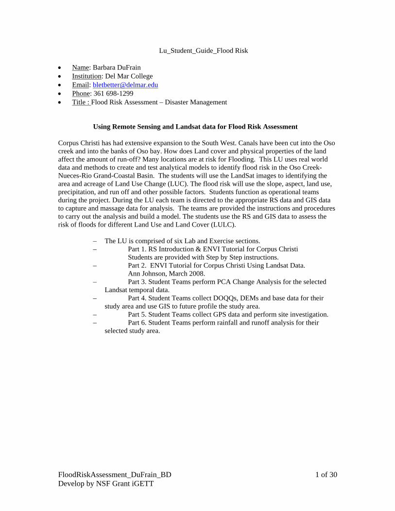
Three steps
• Select Band 1: _b10• No display > New display• Load band.
Steps: _b10 New Display Load band
Slide 14
6/22/2008 iGettProject1 14
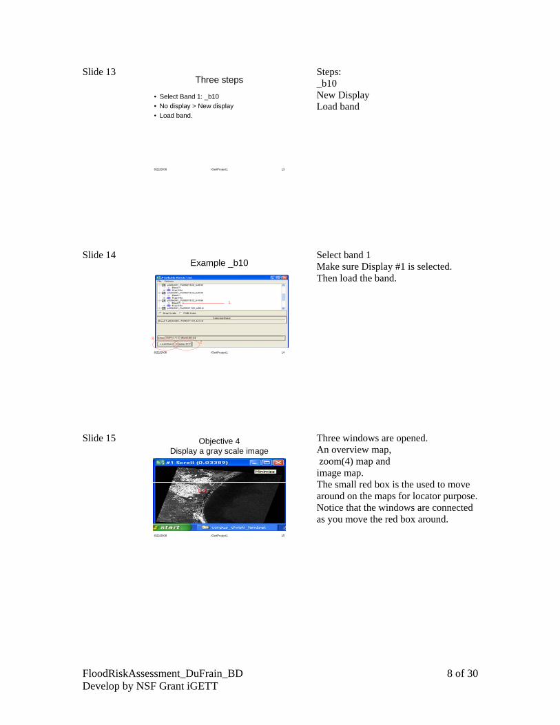
Example _b10
1.
3.2
Select band 1 Make sure Display #1 is selected. Then load the band.
Slide 15
6/22/2008 iGettProject1 15
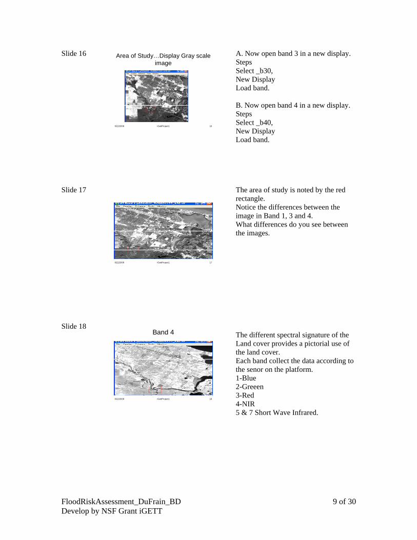
Objective 4Display a gray scale image
Three windows are opened. An overview map, zoom(4) map and image map. The small red box is the used to move around on the maps for locator purpose. Notice that the windows are connected as you move the red box around.
FloodRiskAssessment_DuFrain_BD 9 of 30 Develop by NSF Grant iGETT
Slide 16
6/22/2008 iGettProject1 16
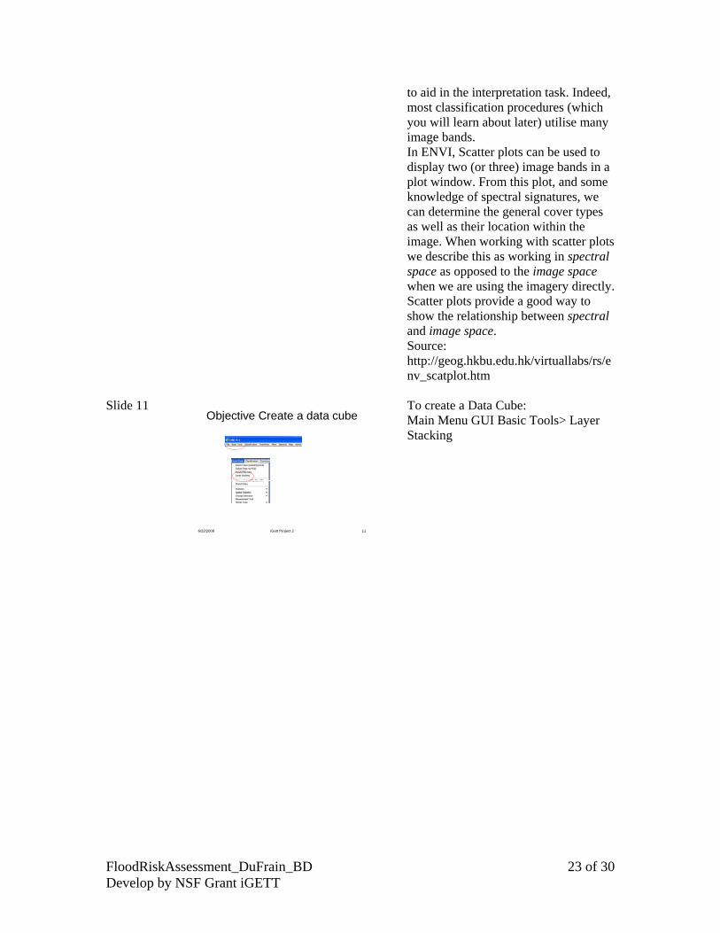
Area of Study…Display Gray scale image
A. Now open band 3 in a new display. Steps Select _b30, New Display Load band. B. Now open band 4 in a new display. Steps Select _b40, New Display Load band.
Slide 17
6/22/2008 iGettProject1 17
The area of study is noted by the red rectangle. Notice the differences between the image in Band 1, 3 and 4. What differences do you see between the images.
Slide 18
6/22/2008 iGettProject1 18
Band 4
The different spectral signature of the Land cover provides a pictorial use of the land cover. Each band collect the data according to the senor on the platform. 1-Blue 2-Greeen 3-Red 4-NIR 5 & 7 Short Wave Infrared.

FloodRiskAssessment_DuFrain_BD 10 of 30 Develop by NSF Grant iGETT
Slide 19
6/22/2008 iGettProject1 19
B61.tif
Notice the Gulf of Mexico.. Click back to the display for _b10.tif and it is black. We are seeing the water depth and particles in it. Band 6 is a good choice if we are examine the gulf. Other bands will help identify exactly what was happening at that day and time.
Slide 20
6/22/2008 iGettProject1 20
B62.tif
Similar to the image in _b61.tif.
Slide 21
6/22/2008 iGettProject1 21
_b70.tif
Crisp and clear. How does this band compare with band 1. You can take a magnifying glass and examine each cell. Fortunately prior research on how the vegetation, urban, wetlands will reflect has been done. The remote sensing software will assist us in analysis. Why Put some theory here.

FloodRiskAssessment_DuFrain_BD 11 of 30 Develop by NSF Grant iGETT
Slide 22
6/22/2008 iGettProject1 22
_b10
Band 1 is the visible: 0.45-0.52 µm :Blue-Green
Slide 23
6/22/2008 iGettProject1 23
Objective 4.Look at the header information
In the Available Bands List, click on the + sign. Example follows
Slide 24
6/22/2008 iGettProject1 24
Map Info _b10
Example. Click on the “+” sign next to the MapInfo

FloodRiskAssessment_DuFrain_BD 12 of 30 Develop by NSF Grant iGETT
Slide 25
6/22/2008 iGettProject1 25
Map Info _b61
Repeat the procedure and examine the MapInfo for band 6 and band 8. Band 6 : 10.40-12.50 um : Thermal IR
Slide 26
6/22/2008 iGettProject1 26
Map Info _b8
Slide 27
6/22/2008 iGettProject1 27
Edit Envi Header
Under the main menu bar go to File > Edit Envi Header

FloodRiskAssessment_DuFrain_BD 13 of 30 Develop by NSF Grant iGETT
Slide 28
6/22/2008 iGettProject1 28
Edit band 1
1
2
In the Action GUI select a band. Then select Okay.
Slide 29
6/22/2008 iGettProject1 29
Results
Your display should reflect the same information.
Slide 30
6/22/2008 iGettProject1 30
Step 2. Edit geographic attributes.
In the Action Window select, 1. Edit Attributes then 2. Geographic corners.

FloodRiskAssessment_DuFrain_BD 14 of 30 Develop by NSF Grant iGETT
Slide 31
6/22/2008 iGettProject1 31
Step 2. Geographic corners.
Notice you can change to Decimal Degrees and vice versa. Cancel the Geographic corners dialog box. Cancel the Header Info dialog box. Click Cancel and Close the display windows.
Slide 32
6/22/2008 iGettProject1 32
Objective 5.Display an RGB Image
• Digital cameras• Incoming visible light• Color filters pass most of their own color
A digital camera produces color images by measuring the brightness level in three roughly equal contiguous ranges. There three ranges are designate green, red and blue bands for convenience. In fact the contain wavelength the eye perceived as a range of distinct colors. The wavelength perceived a violet for example would be included in the visible blue band. Remote Sensing for GIS Managers, Stan Aronoff, , 2005 page 135.
Slide 33
6/22/2008 iGettProject1 33
Available bands list
In the Available Bands list GUI select the “RGB” radio button. Then Select bands 3, 2, 1

FloodRiskAssessment_DuFrain_BD 15 of 30 Develop by NSF Grant iGETT
Slide 34
6/22/2008 iGettProject1 34
Bands 3, 2, 1
Select the bands 3, 2, 1 for Red, green, blue. The natural color composite (Bands 1, 2, and 3), shown below, is a roughly realistic rendition of this scene as it might appear from the air.
Slide 35
6/22/2008 iGettProject1 35
Another Display RGB Image
Bands 3,2,1 image.
Slide 36
6/22/2008 iGettProject1 36
4,3,2 Bands
Select (1) New display and (2) place in Display 2. The above is a false color composite (Bands 2, 3, and 4) . The False color composite refers to coming of several bands of photography with colors that do not replicate normal human vision.

FloodRiskAssessment_DuFrain_BD 16 of 30 Develop by NSF Grant iGETT
Slide 37
6/22/2008 iGettProject1 37
Bands 7,4,2
Select Bands 7,4,2. Load image in Display 2. The 7,4,2 is Pseudo or true color. Blue for the water, green for vegetation and sandy or brown for the plowed fields.
Slide 38
6/22/2008 iGettProject1 38
Bands 4, 5, 3
Load image in display 2. then display. Examine the two images.
Slide 39
6/22/2008 iGettProject1 39
Objective 6.Perform Image Enhancement Image GUI-
In the Image GUI, select Enhance > [Image] Linear.

FloodRiskAssessment_DuFrain_BD 17 of 30 Develop by NSF Grant iGETT
Slide 40
6/22/2008 iGettProject1 40
Linear Stretch
In stretch yields an image having improved contrast near the peaks of the original histogram at the expense of contrast in the darker and lighter potions of a scenes. Also, some image feature characteristics are generally enhanced at the expense of others.
Slide 41
6/22/2008 iGettProject1 41
Linear 0-255
Repeat the process using Linear 0-255, and the others listed below. Note the subtle variation of color on the images.
Slide 42
6/22/2008 iGettProject1 42
Linear 2%
Quite a bit of color change. Remember this is the same image. The power of Remote Sensing is it allow us to tweak an image using different bands to examine our study area. Student repeat with Guassian, Equalization, and Square Root. A. In Image GUI, select Enahance >Interactive Stretching B In Action GUI, Select Stretch_TYPE>Guassian>Apply Repeat with the Equalization and Square Root.

FloodRiskAssessment_DuFrain_BD 18 of 30 Develop by NSF Grant iGETT
Slide 43
6/22/2008 iGettProject1 43
Objective 7. Link Displays
• 3,2,1 • 4,5,3
Have the students display 3,2,1 in Display 1. Near color 4,5,3 in Display 2. Available water
Slide 44
6/22/2008 iGettProject1 44
Tools-->Link-->Link Displays
Crop this one…
Slide 45
6/22/2008 iGettProject1 45
Action GUI
Make sure they say “YES”. Click okay.

FloodRiskAssessment_DuFrain_BD 19 of 30 Develop by NSF Grant iGETT
Slide 46
6/22/2008 iGettProject1 46
Move the red box around.
Slide 47
6/22/2008 iGettProject1 47
Review
1. Introduced Landsat2. Opened a Landsat scene:3. Displayed a gray Scale image?4. Examined the header information?5. Displayed an RGB and others6. Perform Image Enhancement7. Link Displays.
In review. You have been introduce to the Remote sensing and some of the required skills necessary to use the tool. Great Job: Coffee Break. Time
Exercise 2. Slide 1
6/22/2008 iGett Project 2 1
RS-Becoming Familiar

FloodRiskAssessment_DuFrain_BD 20 of 30 Develop by NSF Grant iGETT
Slide 2
6/22/2008 iGett Project 2 2
Objective- The student will be able to ,
• Identify pixel values• Find a pixel location• Measure distance• Display interactive scatter plot• Create and rename a data cube• Overlay vector file.
Slide 3
6/22/2008 iGett Project 2 3
Linked Displays
Students need to repeat link displays from Project 1 to continue. How do we link displays? Have students display #1 bands 3,2,1. display #2 bands4,5,3
Slide 4
6/22/2008 iGett Project 2 4
Objective 1. Cursor location and value
Move your cursor around the image GUI and watch the values change in the action GUI

FloodRiskAssessment_DuFrain_BD 21 of 30 Develop by NSF Grant iGETT
Slide 5
6/22/2008 iGett Project 2 5
Cursor Location and Valid Value
Ask students what the pixel value represents.
Slide 6
6/22/2008 iGett Project 2 6
Slide 7
6/22/2008 iGett Project 2 7
Objective 2. Pixel locator
Now that the students are more comfortable with the interface: 1. In the image GIU, select Tools > pixel locator 2. In the action GUI, Select DDEG 3. Enter the following lat 27.77 N Lon 97.5 W 4. Where are you?

FloodRiskAssessment_DuFrain_BD 22 of 30 Develop by NSF Grant iGETT
Slide 8
6/22/2008 iGett Project 2 8
Where are you?
Slide 9
6/22/2008 iGett Project 2 9
Measure distance
Measure Distance In the image GUI, select Tools> Measurement Tool In the Action Display Measure GUI select Units >Km On the Image GUI, double lick on the airport, then click on the edge of the Bay What’s your distance? Change Units in the Units Menu
Slide 10
6/22/2008 iGett Project 2 10
Display Interactive Scatter Plot
Intereactive Scatter Plot Int the image GUI, select Tools> 2 D Scatter Plots Select a band for X and Y, select Okay Between Band Comparisons: Scatter Plots By now you should be familiar with spectral signatures and what they represent. They allow us to determine regions of the electromagnetic spectrum which are suitable for discriminating between cover types. For example, the NIR region (band 4) is particularly good for identifying vegetation as it generally appears far brighter than other cover types. It is sometimes useful to be able to compare two (or more) spectral regions (bands)
FloodRiskAssessment_DuFrain_BD 23 of 30 Develop by NSF Grant iGETT
to aid in the interpretation task. Indeed, most classification procedures (which you will learn about later) utilise many image bands. In ENVI, Scatter plots can be used to display two (or three) image bands in a plot window. From this plot, and some knowledge of spectral signatures, we can determine the general cover types as well as their location within the image. When working with scatter plots we describe this as working in spectral space as opposed to the image space when we are using the imagery directly. Scatter plots provide a good way to show the relationship between spectral and image space. Source: http://geog.hkbu.edu.hk/virtuallabs/rs/env_scatplot.htm
Slide 11
6/22/2008 iGett Project 2 11
Objective Create a data cube
To create a Data Cube: Main Menu GUI Basic Tools> Layer Stacking

FloodRiskAssessment_DuFrain_BD 24 of 30 Develop by NSF Grant iGETT
Slide 12
6/22/2008 iGett Project 2 12
Action window
Select Import file
Slide 13
6/22/2008 iGett Project 2 13
Create a data cube using
Band 7 from the 1992, 1997 and 2002 data sets.
Slide 14
6/22/2008 iGett Project 2 14
Select the files and Import.
Choose a file name cc-subset-7-data. Then press okay.
FloodRiskAssessment_DuFrain_BD 25 of 30 Develop by NSF Grant iGETT
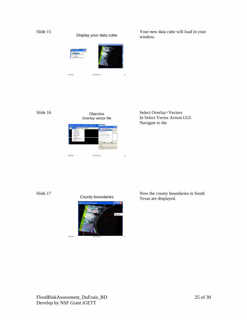
Slide 15
6/22/2008 iGett Project 2 15
Display your data cube
Your new data cube will load in your window.
Slide 16
6/22/2008 iGett Project 2 16
ObjectiveOverlay vector file
Select Overlay>Vectors In Select Vector Action GUI. Navigate to the
Slide 17
6/22/2008 iGett Project 2 17
County boundaries
Nueces
Now the county boundaries in South Texas are displayed.

FloodRiskAssessment_DuFrain_BD 26 of 30 Develop by NSF Grant iGETT
Slide 18
6/22/2008 iGett Project 2 18
Hurray…you did it.
Slide 19
6/22/2008 iGett Project 2 19
Recap-review
• Identify pixel values• Find a pixel location• Measure distance• Display interactive scatter plot• Create and rename a data cube• Overlay vector file.
In this section the student Identify pixel values Find a pixel location Measure distance Display interactive scatter plot Create and rename a data cube Overlay vector file.
Section 2 Is the PCA Change Analysis section using 1992, 1997 and 2002 data. Exercise 3. Principal Component Analysis PCA was invented in 1901 by Karl Pearson[1]. Now it is mostly used as a tool in exploratory data analysis and for making predictive models. PCA involves the calculation of the eigenvalue decomposition of a data covariance matrix or singular value decomposition of a data matrix, usually after mean centering the data for each attribute. The results of a PCA are usually discussed in terms of component scores and loadings[ Source: Wikipedia. Perhaps another definition may help us understand why we wish to perform a PCA Change Analysis. Principal components analysis (PCA) is a statistical mathematical technique to find trends and patterns in highly correlated datasets. In Remote Sensing a PCA will identify and remove redundancy between image data sets. Remote Sensing for GIS Managers by Stan Aronoff has an excellent discussion and example images on pages 302-306. Students follow the steps listed below and perform a PCA Change Analysis using Landsat Data 1992, 1997 and 2002 `
1. Open Band 7 from the 1992, `997 and 2002 data sets. 2. Create a data cube form these three files

FloodRiskAssessment_DuFrain_BD 27 of 30 Develop by NSF Grant iGETT
3. In Main Menu GUI, select Transform > Principle Components > Forwarrd Rotation> Compute statistics and rotate
4. In PC Action GUI, select your three band data cube 5. Enter a name for your statistics file 6. Enter an output file name 7. Click Okay 8. Load all three new bands in separate different grey scale display windows 9. Look at Band 2, notice dark area 10. Open and load a band 4 and 2 from both the 1992 and 2002 data sets.
Create 7,4,2 band combinations for each year, load into separate display windows, then compare dark area found in your PCA which two time epoch 7,4,2 images.
Source: iGett presentation Tutorial Laura August 2007.
FloodRiskAssessment_DuFrain_BD 28 of 30 Develop by NSF Grant iGETT
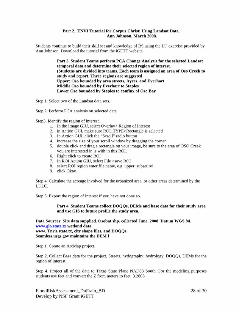
Part 2. ENVI Tutorial for Corpus Christi Using Landsat Data. Ann Johnson, March 2008.
Students continue to build their skill set and knowledge of RS using the LU exercise provided by Ann Johnson. Download the tutorial from the iGETT website.
Part 3. Student Teams perform PCA Change Analysis for the selected Landsat temporal data and determine their selected region of interest. (Studetns are divided into teams. Each team is assigned an area of Oso Creek to study and report. Three regions are suggested. Upper: Oso bounded by area streets, Ayres. and Everhart Middle Oso bounded by Everhart to Staples Lower Oso bounded by Staples to conflux of Oso Bay
Step 1. Select two of the Landsat data sets. Step 2. Perform PCA analysis on selected data Step3. Identify the region of interest.
1. In the Image GIU, select Overlay> Region of Interest 2. in Action GUI, make sure ROI_TYPE>Rectangle is selected 3. In Action GUI, click the “Scroll” radio button 4. increase the size of your scroll window by dragging the corner 5. double click and drag a rectangle on your image, be sure to the area of OSO Creek
you are interested in is with in this ROI. 6. Right click to create ROI 7. In ROI Action GIU, select File >save ROI 8. select ROI region enter file name, e.g. upper_subset.roi 9. click Okay.
Step 4. Calculate the acreage involved for the urbanized area, or other areas determined by the LULC. Step 5. Export the region of interest if you have not done so.
Part 4. Student Teams collect DOQQs, DEMs and base data for their study area and use GIS to future profile the study area.
Data Sources: Site data supplied. Osobat.shp. collected June, 2008. Datum WGS 84. www.glo.state.tx wetland data. www. Tnris.state.tx, city shape files, and DOQQs. Seamless.usgs.gov maintains the DEM f Step 1. Create an ArcMap project. Step 2. Collect Base data for the project, Streets, hydography, hydrology, DOQQs, DEMs for the region of interest. Step 4. Project all of the data to Texas State Plane NAD83 South. For the modeling purposes students use feet and convert the Z from meters to feet. 3.2808

FloodRiskAssessment_DuFrain_BD 29 of 30 Develop by NSF Grant iGETT
Step 5. Create a model for the investigation the data. Use the geoprocessing tools elevation, slope, aspect, and contour. Identify all areas that have an 0 elevation, 5 inch, 10 inch elevation. Step 6. Add the Landsat region of interest to the ArcMap project.
Part 5. Student Teams collect GPS data and perform site investigation. Step 1. Identify the data elements collected (all teams). Create a geodatabase for the data. Geographic WGS84. Step 2. The student selects the GPS software they wish to use.
a. Build new feature dataset to collect the data, open ArcMap and export the region of interest DOQQs
b. Using ArcPAD create new shape file and an a data collection form. c. Use Trimble software and define your datasets.
Step 3. Students are assigned section of Oso Creek to collect the data. GPS are used on the field trip to record information for site verification and examination. Step 4. Students locate base elevation for the bottom of the channel for strategic positions. Step 5. In the office student teams upload and share the data collected
Part 6. Student Teams perform rainfall and runoff analysis for their selected study area.
Data Provided. Runoff data. Curve 1. Barbinfo.doc CN-paper.pdf, Final Tables-NRG.doc Curve: 2 OSO CN.xls, unrdstalb.shp, unrcppalb.shp The Natural Resource Service has develop a method of computing runoff.. Runoff = Curve numbers * Area * Precipitation. There are curve numbers for different soil, slope and land use. The curve numbers developed by the state compute flows using the Oso Creek Watershed. These are based upon historical stream flow at selected gages. Source Sephen Densore Hydrologis TCEQ. Texas Commission for Environmental Quality.. Step 1. Students examine the rainfall and runoff curves that have been developed by the State of Texas to determine the amount of inflows for the Oso Creek-Nueces-Rio Grande-Coastal Basin. The curve numbers are a method of computing runoff.
Runoff = Curve number * Area * Precipitation The curve number selected is based upon soil, slope and Land Use. Step 2. Students investigate and discuss the Water Availability Model (WAM) for Oso Creek-Nueces-Coastal Basin. published by PBS&J to determine the Runoff from an area. Step 3. Students read and extrapolate from the study on ”Updating the NRC Number in the Houston, Galveston area using Landsat data”.

FloodRiskAssessment_DuFrain_BD 30 of 30 Develop by NSF Grant iGETT
Step 4. Students download precipitation data for the two weeks before the date of the Landsat images. Student will identify the three days of rainfall to use for a the following exercise. Depending on where it rained it can take up to 6 days for the water to reach the lower Oso. Step 5. Student will compute the runoff for these areas for pre-urbanization and current LU. Step 6. Pre urbanization-Students will take the NRC computer flow and use the USGS Stage-discharge-curve to find the water height in the Oso channel. Simpliefed for instructional purposes. Day1 will be the base data, day 2 will be after a rainfall. Step 7. Urbanization-Students will take the NRC computer flow and use the USGS Stage-discharge-curve to find the water height in the Oso channel. Simpliefed for instructional purposes. Day1 will be the base data and day 2 will be after a rainfall for urbanization Step 8. Students compare the before and after height of the water level in the channel. Step 9. Students will approximate the elevation of the water from the height of the water and the elevation derived in the field data collection. For instructional purposes this is an idealistic concept. Step 9. Students download the precipitation data for summer 2007 floods on the Nueces River and determine the water elevation for one of the floods. Step 10. Students use the same precipitation data for the NRC computed flow for pre and urbanized. Step 11. Student display their findings in an ArcMap project.