fl~j - library and archives canada · 2004-11-29 · computed/caliirated cv' s of different...
TRANSCRIPT

The Hydrauiics of Buried Streams
by Md Rizwanul Bari
A Thesis Submitted to the Facuhy of Engineering
m Pamai FIlimiment of the Requirernents for the Degree of
MASTER OF APPLIED SCIENCE
Major Subject: Civil Engineering
(Dr. David Hbsen) Department of Civil Engineering, T'UNS
(Dr. M. G. Satish) Department of Co Enginee g, TUNS
fl~J (Dr. M. Salah)
Centre for Water Resources Studies, TUNS
TECHNICAL UNIVERSITY OF NOVA SCOTIA
Halifax, Nova Scotia

National Library I * B c-da Bibliothèque nationale du Canada
Acquisitions and Acquisitions et Bibliographie Senrices services bibliographiques
395 WeIlurgton Street 395, rue Wellington OttawaON K l A W OttawaON K 1 A W canada CaMda
The author has granted a non- exchisive licence allowing the National L h m y of Canada to reproduce, loan, distri-bute or seil copies of this thesis in microform, paper or electronic formats.
The author retains ownership of the copyright in this thesis. Neither the thesis nor substantial extracts fiom it may be printed or otherwise reproduced without the author's permission.
L'auteur a accordé une licence non exclusive permettant a la Bibliothèque nationale du Canada de reproduire, prêter, distribuer ou vendre des copies de cette thèse sous la forme de microfiche/nlm, de reproduction sur papier ou sur format électronique.
L'auteur conserve la propriété du droit d'auteur qui protège cette thèse. Ni la thèse ni des extraits substantiels de celle-ci ne doivent être imprimés ou autrement reproduits sans son autorisation.

TECHNICAL UNLVERSITY OF NOVA SCOTIA LIBRARY
"AUTHORITY TO DISTRIBUTE MANUSCRIIPT THESIS"
TITLE: The Hydraulics of Burïed Streams
The above iibrary may make available or authorize another hirary to make avaüable individuai photo/micr05 copies of this thesis without restrictions.
Full Name of Author : Md Rizwand Bari
Signature of Author : @- : Date : March27,1997

TABLE OF CONTENTS
LIST OF TABLES .................................................................................................. vii
................................................................................................ LIST OF FIGURES ix
LIST OF SYMBOLS AND ABBREVIATIONS .................................................... xi ACKNOWLEDGMENTS ....................................................................................... xvi
ABSTRACT ........................................................................................................... Xvii
1 . INTRODUCrION ......................................................................................... 1
1.1 General ...................................................................................................... 1
1.2 Objectives ............................................................................................ 5
1.3 Orght ion of the Thesis ......................................................................... 5
2 . HTEJUTüRE REVIEW ......................................................................... 8
2.1 FLOW 'Inrough Porous Media ................................................................ 8
2.2 Overview of One-Dimensional non-Darcy Row Equations ................... .. . - 9
2.2.1 The W ' i equation ....................................................................... 9
2.2.2 The Ergun and Ergun-Reichlet equation .......................................... 12
2.2.3 The Stephawn equation ................................................................. 13
2.2.4 The Martin equation ......................................................................... 14
2.2.5 The McCorquodale equation ......................................................... 15
2.2.6 Synoptic comments on non-Darcy flow equations ......................titi.... 16
............... 2.3 OneDimensional Dynamic Equation for Gradually-Vaned Flow 16
2.3.1 Basic assumptions of graduiiy-varied fiow ...................................... 17
2.3.2 Classification of graduaiiy-varïed flow profiles .................................. 18
2.4 Water Surfàce Rofile Computations for GraduaUy-Varied Flow ................ 18
2.4.1 Profile cumputation by the method of Prasad .................................... 21

.............................. 2.4.2 Profile computation by the standard step method 2 1
......................... ............................ 2.5 Fm-Orda Uncatamty Analysis .... 22
3 . STEADY FLOW TEROUGH B U W D STREAMS ................................ . 27
.............................................................................................. 3.1 htroduction 27
................................. 3.2 Dynamic Equation of Flow Through Buried Streams 27
3.3 Characteristics of Water Surtiice Profles Through Buried Streams ............ 29
4 . MODELING OF WATER SURFACE PROFILES ................................................................ TBROUGH B-D STREAMS 30
............................................................................................ 4.1 Introduction 30
.................................................. ......................... 4.2 Mode1 Formulatition ... 31
............................... 4.2.1 Modeling of profile ushg standard step method 32
4.2.2 Modeling of profile ushg the scheme proposed by Prasad ................ 36
......................................................................... 4.3 Limitations of the Models 37
......................... 5 . CAUBRATION AND EVALUATION OF TEE MODEL 39
.............................................................................................. 5.1 Introduction 39
............................................................ 5.2 Experimental Sehip and Procedure 39
........................................................ 5.3 Characterization of the Porous Media 44
5.3.1 Characterization of individu81 particles ..................................... ... . . 44
........................................................................... 5.3.2 Porosityhoid ratio 47
...................................................................... 5.3.3 Hydraulic mean radius 48
............................................................... 5.4 Caliiratioo of Mode1 Parameters 49
5.4.1 Detemination o f particle sufice area efficiency ............................... 49
................................... 5 A 2 Detemination o f Stephenson's fiction Bctor 50
...................................................... 5.4.3 Comments on values of T, and & 50
.......................................................... 5.5 Depth of flow at the Emergent Face 55
5.6 Cornparison of Simulated and Observecl Water Surface Profiles ................. 60

5.6.1 E f f i of fiction dope calculation method on flow profile .................... .. .................................................. 64
5.6.2 Effect of level of trnrbuience on flow profile ..................................... 65
.................. 5.6.3 EfEèct of cross-sectional variabBy in flow profle ..... . 67
5.7 Application of the Mode1 to a Typical Prototype Rock Drain ..................... 73
APPLICATION OF UNLFORM FLOW EQUATION TO NOIY-DARCY FLOW ............................................................................. 81
............................................................................................... 6.1 Introduction 81
............................................................................................ 6.2 Uniform Flow 82
6.2.1 The MaMmg equetion ..................................................................... 84
6.3 Application of the Mannmg Equation to non-Darcy Flow ProNe Computation .................................................................................. 85
ANALYSIS OF UNCERTAINN IN COMPUTED ........................................................................................ DEYrEl OF FLOW 96
.............................................................................................. 7.1 Introduction 96
.................................................................................... 7.2 Type 1 Uncertainty 97
.......................................................................... 7.2.1 Formulation mors 97
7.2.3 Errors due to spacing of cross-sections ......................................... 99
........................................................................... 7.2.4 Application of 101
................................................................................... 7.3 Type II Uncertahty 107
7.3.1 Components contniuting to uncertainty ............................................................................ in computed dqth 110
................. 7.3.2 Uncertainty analysis by first and second moment methods 111
......................................................... 7.3.3 First-order uncertahty anaiysis 112
7.3.4 Sen- of uncertainty m cornputeci depth to mode1 parameters ........................................................................... 116
................................ 7.3.5 Application of first-order uncertahty eqyations 120
............................... 7.3.6 Uncertahty anah/gs by Monte Cario .cmnila tion 127

7.3.7 Cornparison of anaipes by the first-order and Monte Cado simiilatim methods ...................................................... 134
8 . SUMMARY. CONCLUSIONS. AND RECOMMENIDATIONS .......... 146
8.1 Summaiy and Conchisions ................................................................ 146
8.2 Recommendations .............................................................................. 151
REFERENCES ............................. .. .............................................. 153
APPEIYDIX 1
APPENDIX 2
APPENDIX 3
APPENDIX 4
APPENDIX 5
APPENDIX 6
DERIVATION OF EXPRESSION FOR HYDRAULIC MEAN W I ü S ......................................... 159
DERIVATION OF 1-D DYNAMIC EQUATION FOR STEADY FLOW THROUGH
...................................................... BURIEID STREAMS 162
CHARACTERIZING INDIVIDUAL PARTICLES ......... 167
APPLICATION OF HEC-RAS TO NON-DARCY .................................. FLOW PROFILE SMUIATION ,. 170
DERIVATION OF EXPRESSION FOR CRITICAL REACH LENGTH (k) ............................................ 172
DERIVATION OF FIRST-ORDER UNCERTAINTY EQUATIONS ...................................... 178

LIST OF TABLES
Table 1.1
Table 2.1
Table 2.2
Table 5.1
Table 5.2
Table 5.3
Table 5.4
Table 5.5
Table 5.6
Table 5.7
Table 5.8
Table 5.9
Table 6.1
Table 6.2
Table 7.1 .
Table 7.2
Table 7.3
Table 7.4
Table 7.5
Preferred waste rock properties for rock drains ....................................... 4
Values of Wdkh' constant, W. for different porous media ..................... 10
Hydraulic mean radius, m, for Mixent &e of rocks ............................... 12
Sunmiary of physical characteristics of a siniple of 100 particles ............. 44
Resuits of the calibration for the optimum mode1 parameters ................... 52
Cornparison of particle surfkce area eficiencies ...................................... 53
Ratio of obsened and theoretical exit depths .......................................... 58
IDiaerences between observed and smnilated water &ce profiles ......... 63
Reynolds number for diffient discharges ................................................ 66
Computation for loss or rise in head ....................................................... 72
Assumed value of parameters relating to hypotheticd rock drain ............. 77 Magnitude of various ternis of the energy equation of hypothetical rock drain ........................................................................... 79
SSE's for water &ce pronles simulated by modified mode1 uSmg optimum Manning's n~ ........................................................ 87
SSE's for water surfàce pronles simulated by the
rnodifïed models ..................................................................................... 90
Cornparisons of computed depths ............................................................ 103
Equations for the contributions of different independent ......................................... variables to the uncertainty in simulated depth 114
Percent deviations fiom the observed and mean depths of the upper and lower bounds at mid-point of the mode1 rock drain ................. 121
Computed/caliirated CV' s of different model parameters used in generating total uncertainty bands .......................................................... 124
Statistics used to genenite the mput variables m ........................................................................... Monte Car10 simulation 131
vii

Table 7.6 CompPrison of error bound areas and SSE's by W - o r d a unceitainty a d p i s and Monte Carlo Smulation methods ..................... 140
Table 7.7 Average deviatims fkom the observed depth of upper and lower bounds of Monte Carlo simulation and fi&-order unCertamty adysk ............................................................................... 141
Table 7.8 Average deviations fkom the mode1 sohition of upper and lower bounds of Monte Carlo simulation and W-order uncertahy -sis ............................................................................... 141
Table A3.1 Dimensions of the rock particles dong a, b, and c axes .......................... 167
Table A4.1 Comparison of water d c e profiles under depth-mvariant nM condition ~................................................................. 170
Table A4.2 Comparison of water surfiice profiles under ....................... depth-dependent nM condition ..................................... ... 1 7 1

LIST OF FIGURES
Figure 1.1
Figure 1.2
Figure 2.1
Figure 3.1
Figure 4.1
Figure 5.1
Figure 5.2
Figure 5.3
Figure 5.4
Figure 5.5
Figure 5.6
Figure 5.7
Figure 5.8
Figure 5.9
Figure 5.10
Figure 5.11
Figure 5.12
Figure 5.13
Flow through the rock drains ................................................................ 2
Idealized sections of the most wnnnon waste rock dump ................................................................. types in mountah coal mines 3
Classincation and shape of graduaUy-varieci fiow profiles ...................... 19
Derivation of steady state onedimensional dynamic eqiiation of flow through buried stream ............................................................... 28
..................................... Representation of terms m the energy equation 33
Schematic of the eqerimental setup .................................................... 40
Mode1 rock drain m g l a w d e d fhime ......................... .. ............... 42
................................. Rise in water level with discharge ............... .... 43
.............................. Sample of the porous media used in the expriment 45
Rock particle characterhtion ............................................................... 46
Freguency distri'bution of diameter of randordy selected 100 rock particles ............................................................................. 47
Optimization of sudiace area efficiency. Tc. m the W W s equation ........ 5 1
ûpthization of fiction fkctor. K. m the Stephenson eqpation .............. 51
.............................. Cornparison of observed and theoretical exit depths 57
Depth-discharge cwve for the mode1 rock drain
at the emergent &ce .............................................................................. 60
Comparison of observed and simulated water surface profiles . Friction dope computed by Wilkins' equation ....................................... 62
Cornparison of obsened and simiilated water surfrice profiles . Friction dope wmputed by Stephenson's equation ................................ 62
Specinc energy diagram ihstrating for flow through nomprismatic horizontal open channel ...................................................................... 68
Figure 5.14
Figure 5.15
Figure 5-16
Figure 5.17
Figure 6.1
Figure 6.2
Figure 6.3
Figure 7.1
Figure 7.2
Figure 7.3
Figure 7.4
Figure 7.5
Figure 7.6
Figure 7.7
Figure 7.8
Figure 7.9
Figure 7.10
Figure 7.1 1
QuaiitatÏve response of water surfàce profile to changes m chamiel width for a rectanguiar open chRnnef with no porous media .................. 69
Change of width of the mode1 rock drain dong the fhme ...................... 70
Details patammg to hypothetical rock drain ....................................... 75
Sinnilated wata suifrice profiles through the
......................................................................... hypotheticd rock drain 77
OptÎmization of MannSig's in modified mode1 .................................. 87
LongkuRinal variation in the vahie of MPmring's roughness ............................................... coefficient, n ~ . for the mode1 rock drain 94
Cornparison of observecl and simulated water d c e profiles ............... 95
Computational aror m water surface profile computation ..................... 102
................ L- for wide rectangular channels, applicable for MZ profiles 105
................ L,- for wide rectanguiar channels, applicable for M l pronles 106
Chart showhg the topology of cornmon methods for ................................................. perfiormhg Type II uncertahty -sis 109
Relative contribution of model parameters having equal coefficient of variation to mcerfainty m smnilated profiles . Head loss computed by Wïikins' equation ............................................. 118
Relative contn'bution of model parameters h a h g eqyal coefficient of variation to uncertainty in smnilated profiles . Head l o s computed by Stephenson's equation ...................................... 119
Dennition of upper and lower bomds of computed depths for flow through mode1 rock dram ........................................................ 120
Plots of .cirmilsted water surface profiles by the model f 1 o band from kst-order uncertainty anaiysis . Head l o s computed by WilkSis' equation .................................................................................. 125
Plots of simulated water &ce profiles by the mode1 f 1 o band f%om first-order uncertainty an@& . Head loss computed by Stephenson's equation ......................................................................... 126
Histograms of randomly-generated mput model p aramet ers: Data set 1 .............................................................................................. 132
Histopuns of randomty-generated mput model parameters: ............................................................................................. Dataset II 133

Figure 7.12
figure 7.13
Figure 7.14
Figure 7.15
Figure 7.16
Figure A 2.1
Uncertainty bands for profile 1 generated fiom Monte Carlo simulation and the first-order m&ty anahlgs ............................... ... 136
Uncertahty bands for profile 2 generated Born Monte Carlo simulation and the first-order mcertainty analysk ..................... ... ..... 137
Uncertainty bands for profle 3 generated Born Monte Carlo siundation and the fht-order uncertahty -sis . .. . . .. . . . . . . ... . . . .. .. . .... .... . 13 8
Definition sketch of error-bound area, A,, ........................ .. ................ 139
Plots of coefficient of variation of depth of flow dong the bed of the mode1 rock drain nom the ht-order uncertainty malysk and Monte Carlo .cimiilation ................... ,.. ........................................... 143
Derivation of onedimeflsiod dynamic equation of flow through buried stream under steady state condition ............................... 163
Figure A. 5.1 Derivation of critical reach length, Lc . . . . . . . . . . . . . . . . . . . . . . . . . . . . . . . . . . . . . . . . . . . . - . . . . . - - 1 73

LIST OF SYMSOLS AND ABBREVIATIONS
cross-Sectional area.
hydrautic depth.
top width.
depth of flow.
critical deptà
depth of flow at em~gent fàce.
depth of flow at upstream
depth of flow at downstream
buJk velociry.
average velocity of wata through the voids.
velocity of flow at upstream.
velocity of fiow at downstream.
hydraulic conductivity of the porous media.
rate of change of piezomdric head dong the path of flow.
an empirical coefficient m Wilkins' equation accoimtmg mninly for piuticle shape.
visco&y of water.
hydraulic mean radius.
empirical exponent in Wilkins' equation
empmcal exponent m Willrins' eqyation.
empmcal exponent m Wilkins' equation.
Witkins' constant.
vohune of voids withh a control v o h e containhg a porous media.
surface area of voids of a porous media having total area V.
void ratio.
particf e diameter.
porosity.
particle surfàce area Sciency.
a measwe of how the paxticle m e r s m shape from a sphere.
a factor which accoimts for the surnice devhtions of a rough elfipsoidal rock as compared to a smooth ellipsoid
a fom Darcy-Weisbach Ection factor m Ergun's equation.
Reynolds number.
Ergun's partide Reynolds nrrmber.
kinematic viscosity of water.
permeameter diameter in the Ergun equation.
Stephenson's fiction nictor.
friction factor.
gravitational constant.
empirical exponent m Martin's equation.
empirical coefficient m Martin's equation.
coefficient of dormi ty .
Darcy-Weisbach fiction factor for rock and pemeameter but the wall-effect removed fiom the experbental data m McCorquodaie equation.
Darcy-Weisbach fiction factor for a hydraulicaüy smooth surfàce fimctioning at the same Reynolds number as that associated with a rough in McCorquodaie equation.
channel bed slope.
fiction slope.
Froude number (for graduaIly-varied flow in open channek).
pore Froude number (for non-Darcy fiow through rock drains).
any random variable.
mean of any random variable.

standard deviation of any random variable.
mean of depth of flow.
standard deviaticm ofdepth of flow.
total head loss in any reach due to fiction,
stream bed slope angle.
kinetic energy correction fâctor.
discharge.
unit width flow rate.
specinc energy.
change m depth of flow.
hydraulic paramet ers.
Mannmg's roughness coefficient.
factor of dm. uncertainty in smrmlated depth of flow.
coe5cient of variation of drain width.
coe5cient of variation of discharge.
coefficient of variation of surface area efficiency.
coefficient of variation of Wilkms' constant.
coefficient of variation of particle dismeter.
coefficient of variation of fiction slope.
coe5cient of variation of porosity.
coefficient of variation of Stephenson's fiction fàctor.

ABBREVIATIONS
CV CoeflGcient of variation
FOUA Fi-order mcerfainty -sis
MCS Monte Carlo simuidon
SSE Sum of squareci =or
SSM Standard step method
TüNS Technical University of Nova Scoda
WSP Water surface profle

1 achowiedge with deep gratitude the supervision and support of my supervisor, Dr.
David EIansai throughout my program W o r h g close@ with Dr. Hansen was a pleaswe
and a privilege. 1 also thank him for the care and effort he exercised and the time he spent
m reviewhg the thesis and rendering vahiable suggestions for its miprovement.
It is my pleasure to express my shcere appreciation to Dr. M. G. Satish, Dr. M. Salah, and
Mr. Fred Baechfer for serving as the members of my guidhg commatee. 1 thank them for
reviewing the thesis and providing valuable suggestions for its Bnprovement.
In connection with the experimentd work with the physical model, the assistance provided
by the technical statf; especiany Mr. Blair Nickerson of the Hydraulics Laboratory of
Technical University of Nova Swtia is acknowledged.
1 wodd also Iüre to thank all the feitow graduate students in the Water Resources
Research Group at D 304.
The financial support provided by the Natural Sciences and Engineering Research Council
of Canada is gratefuny acknowledged The hancial support m the fonn of Graduate
Research and Teaching Assis&a.tships provided by the Department of C i d Engineering at
TUNS is also achowledged
Fm@ and most knportantiy, my appreciation goes to my h d y who all stood by my side,
encouragecl me, and gave me moral support during diûïcult times m c o d e s s ways.
Without the inspiration 1 got fiom their humor, warmth and love, 1 could not have the
courage or strength to complete this work or even to attempt it.

This thesis reports the resuits of the expimental and numerical investigations canied out
on various aspects of graduaIly-varied flow through vaticajly unconhed b d streams.
This study is focused on artifiw-created buried streams. Such Stream are formed at
open-pit coal mines m mountainous areas due to the disposal of large qyantities of waste
rock m the vdey terrain, and are oeen refmed to as rock drains. The hydraulic anaiysk
techniques describeci herein are not, however, impli* limaed to streams of artificial
genesis.
A numerical model was developed to sindate non-Darcy water sudice profiles through
buxied streams. The perfofmance of the model under laboratory experimental conditions
was found to be satisfnctory. The model presented uses Wilkms' or Stephenson's
eqyation as the headloss equation It was found that the Willrins and Stephenson
equations performed equally weil m simiilating the experimental water surfàce profiles.
The performance of the numerical model was also evahiated under three different fiction
slope averaging methods name@, the arithmetic average, g e o d c average, and the
harmonic average. Based on the resuhs obtained m this shidy it is suggested that any of
the above-mentioned fiction slope averaging techniqyes can give satisfactory estimates
for flow through rock drains, provided that reach lengths are not excesive.
The behavior of non-Darcy flow profiles under v-g cross-sectional conditions was also
mvestigated, both experiment* and computation@. It was found fiom the
expermienta1 mvestigations that the response of non-Darcy flow profiles under v q b g
cross-section condition was not analogous to open channel flow profiles d e r
smnlar conditions. The disgmüanty m behavior of non-Darcy flow profles and that of
gradua&-varied flow (GVF) m opea channek was found to be m a d y due to the relatively
large loss m head due to fiction in the former case compared to the latter.

For fUy-developed turbulent flow through rockn0s it is usuaily a d that the exit
depth is equal to the crirical depth applicable to non-Daq fiow. It was found in this
study that the observed exit depths for various discharges were not the same as the
theoretical exit depths found Eorn a cntical depth formula. It was also found that the
magnitude of the difference mcreased wiîh mcreasing discharge. The breakdown of a key
asumption of GVF was thought to be the main reason for the difference.
An investigation was also carried out to check whetba a UfLiform flow eqyation, such as
the Mamimg equation, wuld be adapted to non-Darcy flow profle simulation. It was
fomd that the adaptation is compidatiody possible, but wiîh qyaHcations. It was
fond that the roughness characteristics of non-Darcy flow profile diffa significantly &om
that of open channel flow. In order to represent the role of roughness, it is m general
necessary to use a depth-dependent Manning's n~ mstead of a depth-mvariant n ~ .
Robable sources of uncatamty associated with water surface profile smnilation through
rock drains were identifid m this shidy. The uncertainty m SMnilated non-Darcy profiles
associated with crosssection spacing was kvestigated. An equation for the r n m h m
allowable distance that should be used in the numerical model between any pair of sections
was derived Data uncertainties were investigated in detd m this study. In order to
quantify the probable error m the computed depth of flow through rock drains, uncertainty
equations were deriveci. These were developed ushg nrsi-order uncertainty analysis
(FOUA), applied to a number of parameters characterizhg the porous media, and
assunmig rectangular drain geometry. A siniplified form of the total uncertainty equation
was applied to quantify the uncertahty associated with the water h c e profiles
Smulated for the model rock drain. UnceriaHity anaiysis for the model rock drain was also
pdormed by Monte Carlo simuiation (MCS). A cornparison was made for the resuits
obtajned fiom FOUA and those obtained fiom MCS. It was found that the variance
esthates from these two approaches differed somewhat fiom each other. Possible
reasons for the diBirences are discussed.

Future work is mdicated in the areas of unsteadiness m the Bow, dope fidure, and fine
material transport m the drains.

Chapter 1
INTRODUCTION
The generation of huge quantities of waste rock at open-pit mal mines m mountainous
areas necedates the permanent idXihg of some of the vaiiey terrain with deposits of
coarse rockfia Under such circu~~lsfances, three options are generafly considered for the
contmued wnveyance of stream flow (1) diverting the flow around the deposii, by a
cibersion channel (2) diverting the flow unda the deposit, through cutverts, and (3)
allowing the flow to pass through the deposit. From a practical and economic pomt of
MW, the third option is the most cornmody used (Ritcey, 1989). In cases where this
option is employed, the exkthg streams m the valleys become buried streams. The
streams continue to flow through the vaiieys, but under great depths of waste rock, and
over considerable distances, sometimes thousands of meters. These bUned streams, also
lmown as ?ock drains", are not embanlcments in the usual sense because their aspect ratio a w
(height/length) is very different fiom that of a typical embanlcment.
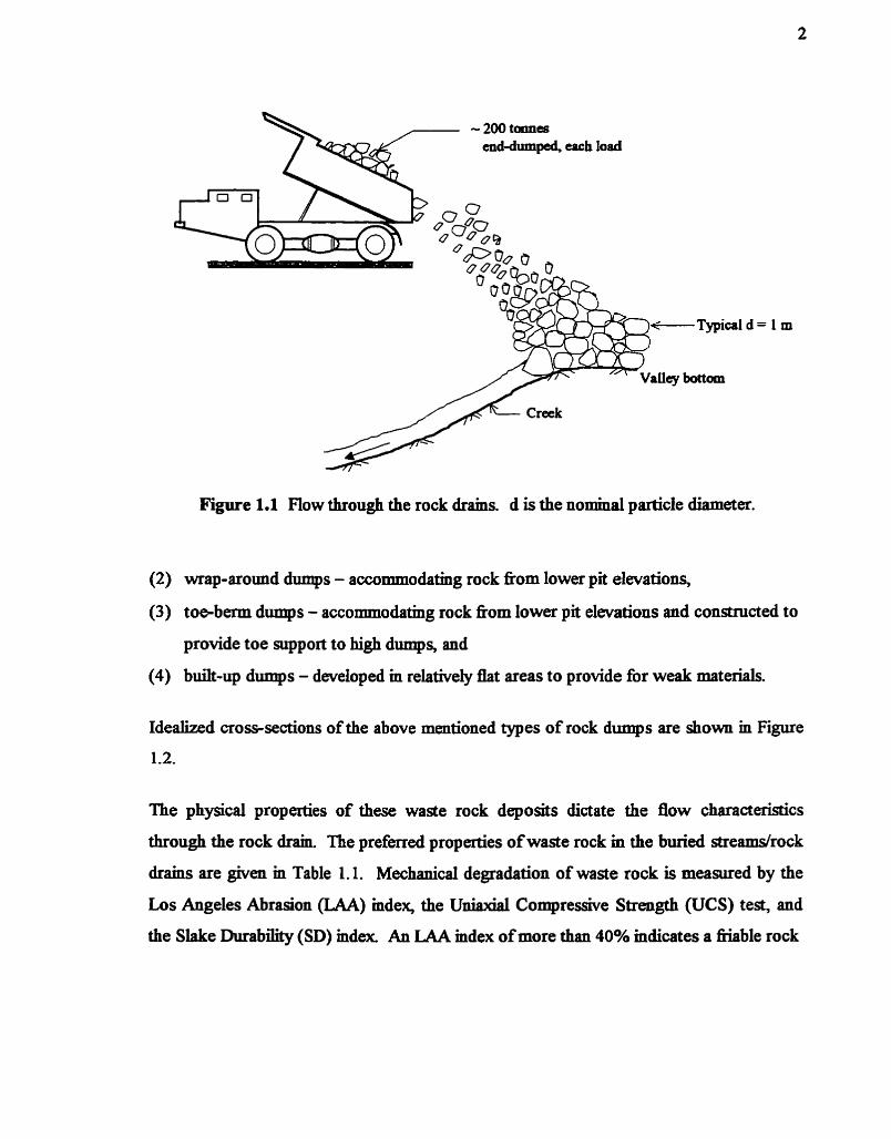
The particIe diameter at the base of these rock drains is ofken about 1 m and iarger, but
decreases graduaiky m the upward direction because the waste rock is deposited by so-
called "end dumping" 6om the crest (see Figure l . l). The depogt is b d t up at the angle
of repose, with the largest particles rolling to the bottom 'Ihae are four conmion types
of dumps comtructed m valleys at coal mines (Ritcey, 1989):
(1) fiee dumps - the highest type, accommodating waste rock fiom pits near mountain
end-dimipab erich load
t-- Typical d = 1 m
Figure 1.1 Fiow through the rock drains. d is the nominal particle diameter.
(2) wrap-around dumps - accommodatmg rock fiom lower pit elevations,
(3) toeberm dumps - accomrnodating rock fiom lower p i elevations and constructed to
provide toe support to high dumps, and
(4) built-up dumps - developed in relatively flat areas to provide for weak materials.
Idealized cross-sections of the above mentioned types of rock dimips are shown m Figure
The physical properties of these waste rock deposits dictate the flow characteristics
through the rock drain. The preferred properties of waste rock Bi the buried s t r e d r o c k
drains are @en m Table 1.1. Mechanical degradation of waste rock is measured by the
Los Angeles Abrasion (LAA) mdex, the Uniaxial Compressive Stmgth (UCS) test, and
the Slake Durability (SD) mdex. An LAA mdex of more than 40% indicates a f?iable rock

Free dump
Figure 1.2 Ideaüzed sections of the most cornmon waste rock dump types in mountah mal mines The numbers indicate the seqyence of dwelopment (der Ritcey, 1989).
*ch win break down into fines during proceshg and dumping. A UCS of more than 50
MPa mdicates a relative@ hard rock which win tend to regst breakdom. An SD mdex of
l e s than 90% indicates the potential for the rock to fiagrnent excesgVely upon exposure
to water.
The relatively rapid flow (as compared to groundwater flow) which moves horizontally
through the base of these deposits does not do so according to Darcy's law, but behaves
m a m e r smiiiar in some ways to open channel flow, because of the very large void
spaces. The longiîudmal variation m water depth dong the buried Stream is, however, no
longer govemed by the roughness of the bed of the stream, as is the case for open channel
fiow, but primarily by the characteristics of the coarse porous media which now fills the
fonnerly open channeL 'Ihere are a number of such bwied streams near open-pit minhg
operations in the Rocky Mountains, particulariy m the Kootenays. The formation of these
buried streams causes permanent local changes in the hydraulic, hydrologie, and Sediment

Table 1.1 Referred waste rock properties for rock drains (afta Ritcey, 1989).
I Cod mines
1 Metalmines Igneous rock
Mechanical Quaiities
I Los Angeles Abrasion index < 40%
U M CompresSve Strength > 50 MPa
1 Physico-Chernieai Qualities
1 Freeze/thaw not significant at bottom of dump
1 Rock Gradation
1 S i fines < 5%
regmies The water surnice elevation along the length of these buried streams greatiy
affects the design, planning, and operation of the mal mines. Also, elevated water depths
m these streams are sometmies associated with largescale dope fidure, particularly at the
downstream toe. It is, therefore, necessary to have a clear understandhg of the
phenornenon that govems the fiow of water through such burïed streams. There should
also be a sound method of computmg the depth of water at different locations along such
streams Although the literature on non-Darcy flow is extensive, there is not a great deal
of information available in the area of gradua.&-varied flow through burieci streams The
work reported herein is an effort to bridge this gap m the study of the flow phenornena
associated with buried streams.

1.2 Objectives
The objectives of this research cm be outlined as foilows:
To dwelop a clear and detaiied statement of the govrrning equations for flow through
buried streams.
To develop a soimd numerical procedure for water &ce profile determination mder
steady state condirions through long depods of coarse porous media, Le., through
rock drains,
To investigate whether the d o m fiow equatiom applicable to gradually-varied open
channel flow, such as the Manning eqytion, cm be applied m some way to the
Smulation of water surfàce profiles wahin buried streams.
To wahiate the uncertainty associated with the computed depth of flow through
buried streams.
This shidy therefore covered two principal areas. First, the development of a numerical
mode1 for water surface profile detemnination through buried streams under steady state
conditions. Second, the identification of the principal sources of errors associated with
water surface profile computation by the numerical mode4 and the dwetopment of
methods to qyantifj~ and nhhize some of these mors.
1.3 Organization of the Thesis
This thesis is organïzed m the following mannec
Chapter 2 contains a literature review of fou. areas important to this çhidy. Section 2.2
reviews some of the work done in non-Darcy flow. Section 2.3 reviews grad*-varied
flow phenornena, its clnssiflcation, and the açsociated assumptions. Section 2.4 explains
the most-commonly used techniques of water surfàce profile computation for open
channel flow. Section 2.5 demies the theory awciated with the hst-order uncertamty
analysis*

Chapter 3 provides a detailed deaivation of the steady state on~dimensional dynamic
equation of flow through buried streams. The procedure fonowed m derivmg the dynamic
equation for flow through bwied streams is smiilar to that of gradually-varied flow.
Chapter 4 provides the mathematical fonmilation of the numerical model for wata surface
profile computation through buried streams under steady state conditions.
Chapter 5 mainiy d e s d e s the performance of the numerical model developed m Chapter
4 m .mnulating water sdhce pronle through buried streams Performance was evaiuated
by comparing the sbulated water surface profles with those obtained from eqeriments
performed on a physicai modeL Section 5.2 provides an outhe of the experirnental setup
and Section 5.3 provides a description of the characteristics of the porous media used in
the eqeriments. The r e d s of the cahbration of the model to obtaÎn the optimum vahies
of different parameters of non-Darcy fiow equations are presented m Section 5.4. Section
5.5 provides a detailed discussion of depth-of fiow at the emergent fice of the rock drain.
Section 5.6 provides the r e d s of a cornparison between observed and Smulated water
sufiace profiles. In Section 5.7 performance of the model under natural condition was
w a b t e d based on hypothetical information. This idormation is carefuIh/ chosen so that
Ït represents a typical rock drain.
Chapter 6 describes the results of the mvestigation canied out in this study relating to the
applicabiiity of the Manning equation in simulating water surfàce profile through buried
streams.
Chapter 7 presents the errorlimcertainty analyses associated with simiilated water surface
profiles through buried streams by the numerical modeL Mirent types of mors are
identifiecl m Section 7.1. Sections 7.2 and 7.3 d e m i e the quantification and mmimiïstion
techniques associated with some of these errors.

F i , Chapter 8 summerizes the miportant outcornes of this study and provides some
suggestions for fimire research.

Chapter 2
LITERATURE REVIEW
2.1 Flow Through Porous Media
For many decades the hydrauiics of flow through porous media has beai based on a simple
law proposed by Henri Darcy in 1856. This empincaily obtahed iaw relates buIk velocity
and hydraulic gradient. Darcy's Law postdates a linear relationship between these
quantities, and may be expressed as:
where:
U : buUc velocity (dimensions UT),
K : hydraulic conductivity of the porous media (dimensions LIT),
i : rate of change of piemmetnc head dong the path of fiow (dimensionless).
When ushg Darcy's iinear law for flow through coarse porous media, it is necessary to be
aware of the mapplicability of this 'îaw" at high Reynolds numbers, den viscous forces
are not the sole reason for energy losses. Examples of cases where Darcy's law does not
tend to hold are fiow through coarse mers, flow through mine waste dumps (especdly
rockfill dumps), and flow m coarsegrained asuifers under high drawdown. For
me-@ analysis of flow systems m these cases, a non-heu velocity versus gradient
relationship must be used, d e s s the Reynolds number is very low.
Revious theoreticai studies have shown that there is no distinct and consistent upper linnt
beyond which Darcy's linear law becomes invalid As m pipe flow, it has been customary

to employ the Reynolds numbq Re, for malring the distinction between b a r (Iiminu)
and non-linear (nirbulent) flows. In practice, the linear flow assumption is valid as long
as Re is less than some fPidv arbitrary value. This critical Re may have any vahie between
1 and 10 (Sen, 1989), dependmg on how Re is defhed for porous media. Hence, there is
no unique vahie for a given type of mataial, and fùrthermore, this Reynolds number is
mdicative of a aansition to turbulent flow which is gradual, and which cannot be Smply
related to porogty.
2.2 Overview of One-Dimensional non-Darcy Flow Equations
High velociîy flows through warse porous media, such as through rockfil dumps, are
usuaUy refmed to as non-Darcy flows (McCorquodale et al., 1978). It is clear that for
non-Darcy flows the relation between U and i becornes non-iinear, taking eitber a
power law form, i = auN (where a is an empmcal constant determined by the properties of
the fhid and of the porous medium, and N is an exponent between 1 and 2) or a quadratic
form, i = SU + tu2 (S and t behg empmcal constants determined by the properties of the
fhid and the medium). Both the power and quadratic forms are used extensive& m
descri'bing onedimensional non-Darcy flow phenornena. Some of the well-known and
widely used non-Darcy flow equations are reported in the folIowing sections. Hansen et
al. (1995) have provided a brief review of these equations.
2.2.1 The Wilkins equation
Wilkins (1956) found that the flow of water through coarse r o c m depends on a number
of fàctors and proposai a power fimction of the following form to d e s d e flow through
coarse porous media:
where:
UV : average v e l o e of water through the voids,

C : an empirical coacient accounting mady for particle shape,
: the viscosity of watq
m : hydraulic mean radius of the coarse porous media,
I : hydraulic gradient,
a, b, & w : empirical exponents.
Based on experimeotal work done m a large packed cohmm, WiIkins reduced equation
12.21 t O the foilowing dimensiondy unbalanced equation:
where:
W : Wilkins' constant.
The product wmo3 in equation [2.3] can be thought of as a hydraulic "conductivity" of
the porous media, as opposed to a hydraulic c'reSsiance" fictor. The eqonent 0.54
mdicates that this eqpation is d e d to the flow regime of neariy-fis&-developed
turbulence.
Wilkins (1956) detemined W nom his data and recommended the foIlowing values as
reported m Table 2.1.
Table 2.1 Values of Wilkins' constant, W, for diff"ent porous media.
Knowing that UV = Uln, where n is the porogty, equation [2.3] can be expressed as:
Units of void velocity &
hydrauiic mean radius
misec & m
in/sec&m
Wilkins' constant, W
Crushed grave1
5.24 mlnlsec
32.9 mIn/sec
Polished marbles
7.33 mlnlsec
46.5 minlsec

The hydraulic mean radius (m) in equatiom [2.2], [2.3], and [2.4] is a rneasure of the
average pore diameter and therefore has a direct bearhg on the quantity of flow which
may be expected to pass through a coarse porous media ( S a h and Hansen, 1994). The
fimdamental dennition of hydradic mepn radius is (Taylor, 1948):
where:
V : vohme of voids within a control volume containhg a porous media,
S, : surface area of voids having total volume V .
Ractical determination of m is possible for clean, monosized rocks but is more uncertain
for weil-graded or non-homogeneous rockfill because of the associated es m
det-g V and, especiany, Sr. Hansen (1992) proposed the following equation for
the determination of m (see Appendix 1 for derivation):
where:
e : void ratio of the porous media,
d : particle dirimeter,
ï. : particle surface area efficiency.
Wïth r, = 1, equation [2.6] is anaiytically tme for a porous media consishg of uni-sized
spheres, when the SUrfjlce ara of the voids lost to mter-particle contact is neglected.

Sabm and Hansen (1994) suggested that Te may be apportioned between two attributes of
a particle, and can be evahmted by the folowhg equation:
where:
R a b k : a measure of how the particle mers m shape fiom a sphere,
Rmo* : a âctor which accoimts for the surface deviatiom of a rough ellipsoidal rock as
compared to a smooth ellipsoid
For a porous media made up of monoshed rocks, with a specific gravity of 2.87, a void
ratio is 1, and using the e q h e n t a l data presented by Wilkms (1956) on particle surface
area, the followhg values of m may be computed:
Table 2.2: Hydraulic mean radius, m, for Mirent Sze of rocks.
Hydradc mean radius (m)
Garga et al. (199 1) reported Te values of about 1.80 for crushed limestone.
2.2.2 The Ergun and Ergun-Reichelt equation
The Ergcm ecpation (Er- 1952) for onedimensional non-Darcy flow may be expressed
as:

where:
f : a fom of Darcy-Weisbach fiction factor = id
u2 12g ' R ~ Q , : Ergun's particleReynolds number = Ud/v,
v : kinematic viscosity of water,
d : particle diameter.
The Ergun-Reicheh e~uation (see Fand and Thinaicaran, 1990) for non-Darcy flow may be
expressed as:
where:
D = permeametez diameter.
The M parameter ailows for the weii-known waIl effect, whereby fhiid shows some
preferential flow next to the permeametex w d
2.2.3 The Stephenson equation
By analogy to flow in conduits, Stephenson (1979) assumed that head loss should be
proportional to u2/n2gm Smce the hydrauiic mean radius, m, is proportional to the stone
Sze by equation [2.6], Stephenson suggested that the hydraulic gradient for flow through
coarse porous media may be expressed as:
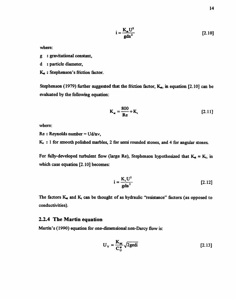
where:
g : @ational constant,
d : particle djameter,
& : Stephenson's friction fàctor.
Stephenson (1979) fiuther suggested that the fiction Bctor, &, m equation [2.10] can be
e v h t e d by the foliowhg equation:
where:
Re : Reynolds number = Ud/nv,
K< : 1 for smooth polished marbles, 2 for semi rounded Stones, and 4 for an- dones.
For fiiIly-developed turbulent fiow (large Re), Stephenson hypothesized that & = K, m
which case equation [2.10] becomes:
The factors K, and % cm be thought of as hydraulic "resistance" &dors (as opposed to
conductivities).
2.2.4 The Martin equation
Martin's (1990) equation for one-dimensional non-Darcy flow is:

wher e:
y : empmcal exponent = 0.26,
Cu : coefficient of d o - = Mdla
: empirical we5cient = 0. S6/O. 75 for angularlrounded materials, respective@'
e : void ratio.
Equation [2.13] is valid for Martin's Reynolds number, & > 300. The dennition of R a
can be eqressed by:
4U,m Re, = -
v
2.2.5 The McCorquodale equation
McCorquodale et ai. (1978) proposed a general non-Darcy flow equation for coarse
porous media which accounts for particle ske, distr'bution, and shape as wen as &ce
roughness, porosiîy, and the wall effect. This dimensionless equation was developed on
the basis of approximately 1250 permemeter tests, grah sizes varying fiom 55 mm to 79
mm, and the pore Reynolds n d e r & (=Ud/nv) va@g fiom 0.001 to 20,000.
McCorquodale et al. (1978) proposed two different equations for two probable regimes of
non-Darcy flow, name& (i) non-linear Lammar flow, and (ii) transitional-turbulent to fiiny-
turbulent fiow.
The McCorquodale equation may be expressed as (McCorquodale et al., 1978):
(i) for non-hem laminar flow (Rp S 500):
(ri) for transitional-turbulent to fuUy-turbulent flow (Rp > 500):

where:
: Darcy-Weisbach fiiction factor for rock and permeameter but wiîh the wd effect
removed fkom the experimaital data,
f0 : Darcy-Weisbach fiction nictor for a hydraulically snooth surnice hctioning at the
same Reynolds number as that associated with a rough wd( as obtained fiom the
Moody diagram for pipe flow). The ratio of W& is about 1.5 for d e d rock (pers.
wmm, McCorqyodale, 1990)'
m' : effective hydraulic mean radius.
2.2.6 Synoptic comrnents on non-Darcy flow equations
The Ergun, McCorquodale, and Ergun-Reichelt ep t i ons represent generabtions of
large sets of data into W e d equationsflS These data sets mchded the resuits of
researchers other than those to whom the final equation is attributed The MaitEi equation
is based on experiments performed on a moderate range of porous media types but
hchided M e or no data î?om other sources. Both the Stephenson and W W s equations
are based on eqeRments on cnished rocks of a relative@ narrow &range and of a given
an-.
2.3 One-Dimensional Dynamic Equation for Graduaiiy-Varied Flow
GradUany-varied flow (GVF) can be deked as a flow d o s e depth varies grad* dong
the length of the channel (Chow, 1959). Unda such grad* changing conditions the
curvature of the streamlines m GVF is SUfficientiy srnaIl that the change in piezomeûic
head in the direction normal to the streamljnes is neglipile. Under such conditions the
pressure distriiution is hydrostatic in the direction normal to the streamlines.

The g e n d differential equation for graduany-v&ed flow, refmed as the one-dimensi01181
dynamic equation of grad*-varied fiow, or Saipiy as the gra.amially-varied-flow
equation, is very we&known and may be eqressed as (French, 1994):
where:
S, : channel bed dope,
: fiction dope,
h : Froude number of flow = U / 3 3 , U : average velocity through the channei,
D : hydraulic depth of the channeL
Equation [2.1fl represents the dope of the w a t a mfàce, with respect to the bed of a
channel of arbihary shape, as a hction of S, &, and Fr. Equation 12.171 has been
derived on the premise that the velocity distriution across the section is d o m
2.3.1 Basic assumptions of graduaiiy-varied flow
The development of the onedirnedonal gradually-varied flow equation, equation 12. lq, the associated theory and the various solution techniques, are based on the foliowhg
fimdamental assumptions:
1. The fiction dope at a given cross-section under non-domi flow condition cm be
evahiated using a rearranged d o m flow eqyation.
2. The dope of the channel is smalL Therefore the depth of flow is the same whether
it is measured vertically or perpendicular to the bottom
3. There is no air enirainment.
4. The velocity distriiution m the channel section is fixed.

In addition to the above assumptions, the regstance coefficient is usuaIly taken to be
mdependent of the depth of flow and considered to be constant throughout the reach
under consideration.
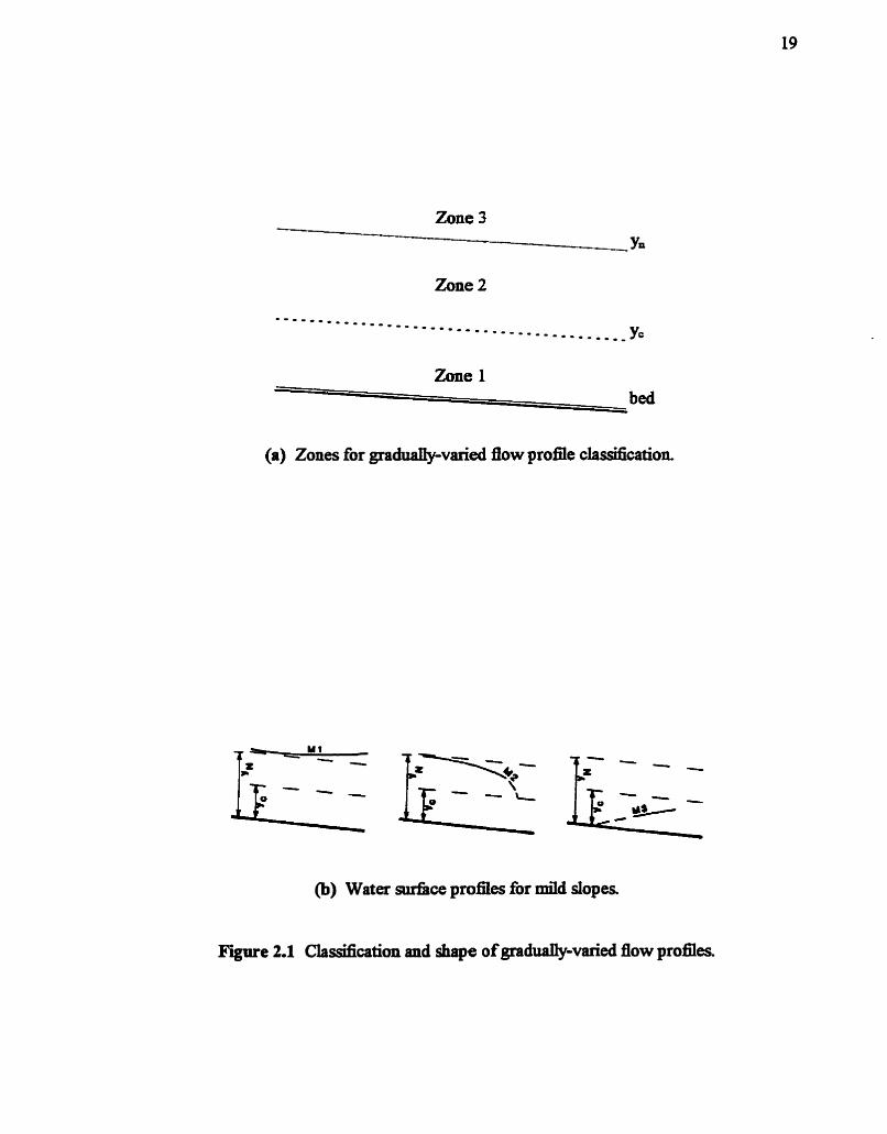
2.3.2 Classification of gradualiy-varied flow profiles
For a @en discharge and channe1 conditions, the nomnal depth, the critical depth, and the
bed M e a channel into the foilowing thne zones in the vertical (see Figure 2.1 a):
Zone 1: The space above the qper line,
Zone 2: The space between the two lines,
Zone 3: The space below the lower line.
The normal depth may be above or below the critical depth, Thus, the flow profiles may
be clas&ed mto thiaeen different types according to the nature of the channel dope and
the zone in which the water surface lies (Chow, 1959). These flow types are designated
as: EU, H3; Ml, M2, M3; Cl, CS, C3; S1, S2, S3; and A2, A3; wfiere the letters are
descriptive of the dopes: H for horizontal dope, M for mild slope, C for critical slope, S
for steep dope, and A for adverse slope; and where numerah represent the zone number.
Profiles H1 and Al are not physicaIiy possible. Of the thirteen flow profiles, tweive
represent cases of graddly-varied flow and one, C2, is a case of d o r m 0ow. The
general shape of the flow profiles for d d dopes is shown in Figure 2.1 b.
2.4 Water Surface Profile Computations for Graduaiiy-Varied Fiow
For gradUany-varied open channel flow, two widely-used wata surnice profile
computation procedures are the method of Prasad (Prasad, 1970) and the Standard Step
Method, SSM (Chow, 1959). The method proposed by Prasad numerically mtegrates the
one dimensional dynamic equation for GVF (eqn. 2.17) at successive sections, starhg
with a known water IeveL In this method, the computation can proceed fiom upstream to
domstream or vice versa, ie. the direction of computation does not depend on whether
Zone 3 a, YU
Zone 2
Zone 1
b e d
(a) Zones for graddy-varied flow profîie classification.
@) Water surfàce profiles for m*l dopes
F'ïgure 2.1 Classification and shepe of graduany-varied flow profiles

the flow is subaiticai or superdcd On the other han& the SSM in GVF profile
computation applies the energy eqyation successively across pairs of sections (at which
the depth at one section is known) and soIves this equation to obtain the unlaiown depth.
The latter is the upstream depth whai the flow is subcriticai.
Smce m aIi but a fw cases a closeù-formed integration of equation 12.1 7J is not possMe,
Ït is necessary to resort to numericd integration procedures. These fiequentIy mvoive
iterative or successive-trial computational schemes (McBean and Parkins, 1975 b).
Numerical integration methods require evafuation of the fimction qy, x) m eqyation [2.171
at a number of discrete pomts y and produce sohmons yj at these points, where j =
l,2,3 ....... N. Among the Smplest numerical mtegration methods are those m which the
sohition at one section, j = 1, is used to generate the sohition at the next section j = j + 1,
as long as a suitable boundary condition of the form y = y, at x = xo is available.
Adopting this simple general method, equation 12.171 can be d e n :
X-xj If we deke: Axj =xj+< -xj, s=- , and y; = f(y, s) , then equation [2.18]
Axj becomes:
I
y,, = yj + ~ x ~ [ ~ , d s O
A whole sub-fhdy of procedures then may be proposed depaiding on the approximation
used to waluate the mtegraL The accuracy and the computational effort associated with
any particular member of this fàndy depends on the form of the approximation which is
adopted (McBean and Parkms, 1975 b).
A particuIarly simple scheme resuhts if the derivative, y, is assumeci to Vary linearly over
the interval, yieIding:

The computational procedure implied by equation [2.21] is often refmed as the
trapezoidal method of integration. Eqyation [2.2 11 was first proposed by Prasad (Rasad,
1970) and demoxutrated to be an usefbl algorithm in water surnice profile computations.
2.4.1 Profiie computation by the method of Prasad
Numerical solution of eqyation [2.21] for GVF for each y*, may be achieved by the
method of successive substitution. This method proceeds nom an niitial asnimption of the
miplicit variable, say y!!. This vaîue is subsequently incorporated hto the right hand side
of the equation, which in turn provides a new depth estimate, y f , * This process is
suxmmkd by the recufsion relation expressed by the foflowing equation (McBean and
Parkhs, 1975 a):
The cycle is repeated, if necessary, mtil two successive estimates agree wahm some
acceptable tolerance.
2.4.2 Profiie computation by the standard step method
The standard step method (SSM) is perfomed by solving an equation based on the totd
head and fiction dope. 'Inis equation is (Chow, 1959):

where:
E& : total head above a datirni at section j,
H,+, : total head above a d a m at section j + 1, Sfj : fiction slope at sections j,
SgI : fiction slope at section j + 1.
Unda the SSM, computations begh with a known depth for a &en discharge at a
specified channe1 section and proceed m the upstream or dowwtream direction, depending
upon whether the flow is subcritical or supacriticat
Both equations [2.22] and [2.23] defhe procedures for the solution at x,+i which are
hqlicit Hi the sense that the ight-hmd side mvolves a temi that is a fùnction of conditions
at that point, Le., the derivative ,or the fiction slope Sf*l . This iniplies that an
iterative procedure must be used to obtain the sohstion represented by either of these
equations.
2.5 First-Order Uncertainty Analysis
First-order uncertainty nnalysis (FOUA) enables an analyst to practicaily and realisticàiiy
mode1 many engineering problems because it works with only the first and second-order
moments of the relevant random variables and processes. The term 'inodehg" m this
context refers to modeling of the uncertainty h the physicdnumerical models and m the
physical parmeters used in these models. In this research FOUA was used to examine the
nature and magnitude of the uncextainties Qi computed wata surnice profiles, as affected
by the imperfiiess of the knowledge of the physical conditions of the channel and the
flow m it (non-Darcy flow m this case).
FOUA (Comell, 1972) is characterized by two fattues: (i) a single moment treatment of
the uncertain or random component, and (8) a ht-order analysis of the hctional
relationships between variables. The fbst feature miplies that the random component (Le.,
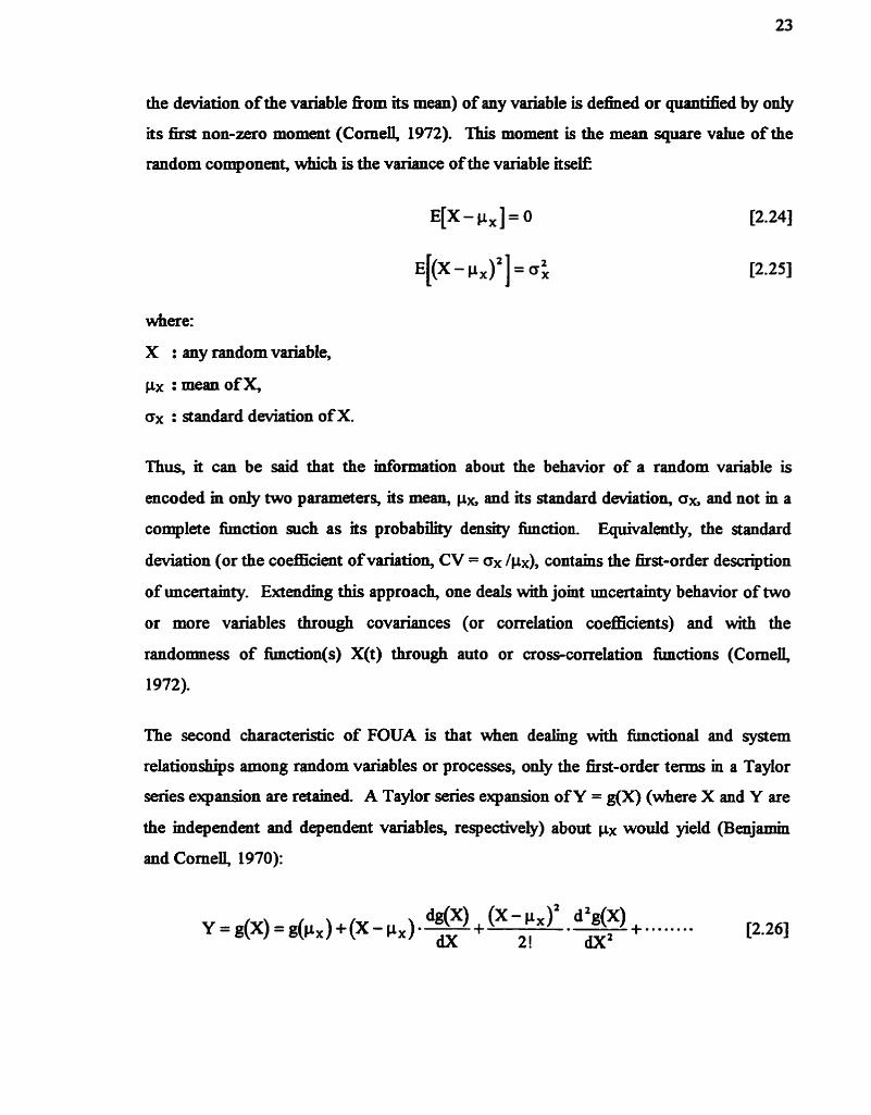
the deviation of the variable fiom its mean) of any variable is de- or ~ u a n s e d by only
its first non-zero moment (CorneIl, 1972). This moment is the mean square vahe of the
random wmponent, *ch is the variance of the variable itseE
where:
X : any random variable,
px : mean of X,
crx : standard deviation of X.
Thus, it can be said that the information about the behavior of a random variable is
encoded in ody two parameters, its mean, ps and t s standard deviation, a% and not in a
complete fimaion such as its probabiüty density function. Equivalently, the standard
deMation (or the coefficient of variation, CV = ox /px), contains the hst-order description
of rmcertainty. Extaidhg this approach, one de& with joint uncertainty behavior of two
or more variables through covariances (or correlation coefficients) and with the
randonmess of fùnction(s) X(t) through auto or cross-correlation fùnctions (Comeil,
1972).
The second characteristic of FOUA is that when dealing with hctional and system
relationships among random variables or processes, only the first-order ternis m a Taylor
series expansion are retained. A Taylor series expansion of Y = gOC) (where X and Y are
the independent and dependent variables, respectiveiy) about px wodd yield (Benjamin
and CorneIl, 1970):

ui order to mvestigate the fimctional relationshq>s betweefl the variables X and Y f?om the
second characteristic of FOU& ody the hear terms are retained fiom the Taylor series
expansion of Y = g0 m eqyation [2.26]. Therefore, to dehe the fûnctional relationship
between the dependent and mdependent variables, the fbt-order approximation of
equation [2.26] iS:
1 The symbol = in equation E2.277 means "equal m a first-order sense". Equation 12.271 can
be expresseci more generaily as:
where:
X : colurnn vector of random variables, -
p : vector of the means of the random variables, -X
Ml-) b : transpose of a cohurm vector of pamal dexivatives: b = - . -
It is ahvays ~de r s tood that equatiom [2.26], 12.271, 12.281 and the expression for bj are
evaluated at the mean, px. Also, ifY(t) is the output of a system operathg on mput X(t),
then under first-order &sis:
where:
: operator ( h e m or non-linear) of the system acting on the mean vahe
function of X(t),

dL - [ ~ ( t ) - Cl (t)] : convoiution of the (linear or hearized) system function and the dx zero-mean deviation process, X(t) -Mt).
It is worthwhile to summarize and -te a number of key took m FOUA for use at later
stages. For the relationship defmed by eqyation [2.27'17 the mean and variance of Y are:
whexe:
x, : covariance matrix of the vector of mdependent variables X .
When thex's are statisticaIiy mdependent eqytion [2.29] reduces to the fhdiar "error
propagation formula":
2 6, =
The relationships between nrst and second moments of linear fùnctions of random
variables are orders-of-magnitude less complicated than those between their fidi
probability distri'bution fùnctions. The disadvantages of FOUA are that the analysis is
mcomplete, and that cefiah relationships of mterest (ie., Y = max [X 1) do not lend
themsehres to this mdysis. Howwer, in many engineering problems these disadvantages
are more than ofkt by several major advantages. One of the advantages of FOUA is that
the iinalysis often mvoives the same tools and procedures of algebra and calcuhrs that are
commonly used m the deterministic analygs of the same problern (ie., matrix algebra and
the convohition mtegration). This advantage is coupled to the major advantage of fïrt-
order anaiysis, which is that the practical feasiiility of andyzing more thoroughly and

richly stochastic models encourages such modehg to take place where it nnght not have
otherwise (Comeii, 1972). It is miportant m engineering applications that the tendency to
model ody those probabilistic aspects that we think we lmow how to a d y z be avoided.
It is us tdy better to have an approximate model of the whole problem then an exact
mode1 of only a portion of the problem

Chapter 3
STEADY n o w THROUGH BURIED STWEAMS
3.1 Introduction
For flow through porous media foflowing Darcy's law, the velocity is d
Consequently, the momentum and km& energy of the floWmg fiuid are negligible. This
is not the case for flow through coarse porous media such as rock drains or buried
streams. The flow phenornena in such cases is analogous to that occurring in open
channek. The fiee surnice profile for steady flow in biaied streams may be determined m
a mariner Smilar to that for flow m open c h e l s .
3.2 Dynamic Equation of Flow Through Buried Streams
Consider an elementary length dx (Figure 3.1) of a gradUany-vaxied fkee surnice fiow
through a reach of buried stream Using the defjnitions shown in Figure 3.1, the one-
dimensional dynamic eqyation of flow through buried strearns under steady state condition
can be shown to be:
Where: T T
h p : pore Froude number of the flow = - ,% The derivation of equation [3.1] is presented in Appendix 2. Equation [3.1] is deriveci on
the premise that a, which takes into account the n o n - d o m velocity distri'bution across a
&en cross-section of buried stream, U m&y.


Eqyation 13.11 expresses the longitudinal surface slope of the fiow through the rocks with
respect to the stream bed. Eqyation [3.1] is similar to the dynnmic w o n applicable to
open channels (eqn 2.17). For the open channe1 case, the tam on the right hand side of
equation [3.1] is computed ussig a d o m flow regstance equation ( u s d y MaimHig or
Chezy), but for buried strems this should be substmited by one of the non-Darcy flow
equations described m Section 2.2. Also, for the open channel case, the pore Froude
number, Fr, in equation [3.1] is replaced by the Froude number, h, of the open channel
flow.
3.3 Characteristics of Water Surface Profiles Through Buried Streams
The dynamic equation for flow through rock drains, equation [3.1], expresses the
lonpmidid surfice slope of the flowing water with respect to the stream bottom It can
therefore be used to describe the characteristics of flow profiles through buied streams.
For a givm vahie of Q, the tenns Fr, and &of equation [3.1] are fimctions of the depth of
flow, y. Both Fr, and &have a strong mverse dependence on the flow area or depth of
flow. In other words, as y inmeases, both Fr, and decrease. Iheoreticdy, turbulent
flow m coarse porous media may be either subdca l or superdcal, but supercritical
flow rarely occurs in rockfiIl (Stephenson, 1979). In aimost aii cases the flow is
subcritical, so that h, cc 1. As a resuh, the sign of dyldx m equation [3.1] is solely
dependent on because S, @ed slope) is fked for a given reach of streslllz Therefore,
when & > S, dy/dx is negative, and the depth of flow decreases with distance. This flow
profile is similar to the M2 drawdown curve of open channe1 Bow (see Figure 2.1 b). Oa
the other hand, when & < S, dy/dx is positive, and the depth of flow increases with
distance. This condition is smiilar to an M l backwater curve in open chamel flow.

Chapter 4
MODELING OF WATER SURFACE PROFTLES
THROUGH BURIED STREAMS
4.1 Introduction
As previoudy mentioned, water sudiace profiles through b d streams can be computed
by numerically mtegrathg the onedimensional dynamic eqyation of flow (eqn. 3.1). In
Section 2.2, some of the works on flow through coarse porous media that have been
reporteci to date were brie* descriid Most of these researches congsted of tests on
d models, constnicted of materials carefùlly screened to a single size. Howwer, the
porous media of natural buriecl streams are not rnonosized and cm be either homogeneous
or non-hornogeneous. It is common m rock drains to have materials ranghg m size nom
rock as large as 1 m m diameter or more at the base, down to fines at the top. As stated m
Chapter 1, rock drains or buRed streams are formed by end-dumping q-ed rocks f?om
the crest of the dump. It is cornmon m mountrim valleys, where the buried streams are
usuaily fonned, for the dump height to be more than 50 m Such large dump heights
result m the segregation of rock particles and this causes parameters relatmg to the porous
media such as porosity, particle diameter, and hydraulic mean radius to be variable m the
vertical direction. Even though the buried streams are of such depth that they usuaily ody
flow through the coarsest materid, estimahg such factors as the hydraulic mean radius
for this coarse fiaction is dBcult, especially whai it is done based on field inspection(s) of
a rock drain andlor rough estimates of the mas, volume, and shape of the visible rocks.
Such variabbüity m porous media characteristics may also be present in the longmidina1
direction of the stream, but is generany a less-severe variation. Whatever the extent and

nature of the variability in porous media characteristics m the longitudinal direction,
accommodating such variabiiity in numerical hydraulic computations is not difEcuh. Such
variabiüty can be accommodated in the numezical computations by changing the respective
media properties in the goveming non-Darcy flow eqyation on a reach-by-reach b a h .
However, it would be diEEcutt to computationaily account for the variab- in the porous
media characteristics in the vertical direction and assign representative values for different
parameters relating to the porous media, as mentioned above.
The practical problem of cornputhg water d c e pronles through bimed streams is
therefore chaIlaighg because of the associated difEcufties m assigning representative field
vahies to the various parameters relating to the porous media and because turbulent flow
in coarse porous media is not completeiy understood Although the possble presence of
d - s i z e d materiais complicates the problem of flow through rocknIis, its significance
may be exaggerated (except poçsiibly for very smaIl fiiis). For example, m many cases, an
estimate of the quantity of flow that is correct w i t h a fàctor of 2 to 5 may be satisnictory
(Lepps, 1973).
4.2 Mode1 Formulation
There are a number of methods found in the literature for integratiag the dynamic equation
for gradUany-varied %ow so as to determine the variation of the depth of flow with respect
to distance. Among the available soiution techniques for accompash8ig this mtegration,
one method may be superior to the others in a particuIar situation. Thus, the user is
cautioned to carefdiy consider the problem before proceedhg to a particular
computational procedure (French, 1994).
As has been stated for the graddly-varied open channel flow, two wideiy-used water
surface profile computation procedures are the standard step method (SSM) and the
method of Prasad (Prasad, 1970). In this study, two different models were developed to

predict water SUifàce pronles throagh buned streams. One made use of a solution
technique Smilar to SSM, and the otha the numerical scheme proposed by Rasad (1970).
4.2.1 Modeling of profile using the standard step method
The application of the energy equation between two adjacent cros+sections of a buried
stream yields (Figure 4.1):
where:
Uvi : void velocity at downstream crowsection (section l),
uvt : void velocïty at upstream crowsection (section Z),
HF : total head loss in the reach due to fiction,
8 : stream dope angle,
al, and a2 : kmetic energy correction fiaor for cross-sections 1 and 2, respectively.
The terni a in eqwtion [4.1] is used to correct the non-dormity of the velocity profile
across the crosîsections. For turbulent flow m open channek with simple cross-sections
the value of a can be as low as 1.05. For non-Darcy flow through rock drains, it is
reasonable to assume a = 1.00, since u2v/2g is very d and the devhtion of the actual
mapitude of a fiom u&y does not Sgnificantiy affect the total magnitude of the term
a ~ ' v / 2 ~ . For an practical purposes, when the stream bed slope angle is smd (ie., when û
< 4') the vahie of cos 0 can be considered to be equai to one. These simplifications (a =
1.00 and cos 8 = 1.00) do not violate the assumptions of graduaily-varied flow stated m
Section 2.3.1. Under such ciraunstances equation [4.1] becomes:


The head loss term (IIF) in equation [4.2] can be approxirnated by:
HF = Sfw DAX
where:
: representative fiction dope for the reach considered,
Ax : distance between the cross-sections.
One @le way to e v h t e the magnitude of S, rg
is by the foilowhg equation:
where:
Sr : fiction dope at crosç-section 1,
S, : fiction dope at cross-section 2.
Substihiting eqyations [4.3] & [4.4] in equation [4.2] yieids:
For convenience, let us define:
Substmmon of eqytions [4.6] & [4.71 mto equation [ 4.51 yields:

As descriied m Section 2.2, an the non-Darcy flow equations can be stated as predictors
of the hydradic gradient, ï, as a function of void velocity and the physicai characteristics of
the coarse porous media If we replace the fiction dope in equation 14-81 by i (found
fkom one of the non-Darcy flow equaticms demiied m Section 2.2), it win be possible to
w h t e the value of HI, aSSuming that the mors d g fkom this subsMution are
nepiigible. Among the non-Darcy flow equations prewioudy demibed, WilkEis' equation
(ecp 2.4) and the Stephenson equation (eqn. 2.10) are easy to use for practical purposes.
W i k i d eqyation is a well lmown and popular equation for flow through coarse porous
media. It is noted that WiIkins' equation has been used m Canada for the evahiation of
flowthrough mine waste dumps at coal mines (Campbell 1989; Lane et ai. 1986). The
accuracy of Wilkins' equation depends mady on being able to evahiate the value of W and
m for the particular porous media being shidied While there is uncertainty about the vahte
of W and m for a given material, the rather lirriired range cited earlier liniits the error in
-sis which might result fkom aich uncatainty.
Substmitmg Wilkins7 equation, equation [2.4], mto equation 14.81 yields:
S w b , subdtuthg Stephenson's equation, equation [2.12], into equation l4.81 yields:
S idaneous solution of equations [4.6] and r4.71 with d e r equation 14.91 or r4.101
leads to the d o w n depth of water at the upstream cross-section. This can be achieved
teratively. Wi the help of Figure 4.1, the computational procedure can be outlined as
follows:

1. Knowing the depth of flow, yl, at the downstream cross-section (cross-section 1) and
the discharge? the velocity head, u2w/2g, is cdculated and equation [4.6] is solved for
HI. The local fiction dope, &, is calculated by eqyation 12.41 or (2.101.
2. A depth of water, y2, is assumed at the upstream crosesection (cross-section 2).
3. Based on the assumed value of y2 m szep (2), the velocity head, u2vt/2g, is calcuiated
and equation [4.7 is sohred for H2. The fiiction dope (&) is calculated again by either
equation [2.4] or [2.10].
4. Shce all the terms on the right hand side of equation [4.9] or [4.10] are known, the
eqyation being used is sohred for Hz.
5. Compare the vahie of H2 found fiom step (3) wiîh that computed in step (4). Repeat
steps 1 through 5 until the values of Ht agree within a pre-dehed tolerance.
4.2.2 Modeling of profile using the scheme proposed by Prasad
Application of equations [2.21] and 13.11 to a pair of adjacent cross-sections of a buried
Stream, as shown in Figure 4.1, yields:
Replacing the tenu & in equation [4.11] by the Wilkius and Stephenson equations, the
following equations can be obtained, a f t s reamangement:

Sohition of d e r of eqyations [4.12] and [4.13] provides the unknown depth of water at
cross-section 1. An the temis in the above two equations with subscript 2, m other words,
the parameters assocbted wiîh cross-section 2, are known at the beghhg of each
iteration, but for the temis with submipt 1, only the channel dope and parameters
associated with the porous media are knowe This leaves velocity, U, and pore Froude
number, h p , at cros+section 1 as unknown quanthies. Smce both U and k p at cross-
section 1 are hct ions of y, (the depth of flow at cross-section l), there is no explkit
soiution to the above two equations for most cases. As a re& an terative sohition
technique must be employed to sohe any of these equations for y*. The mode1 developed
m this shidy sohes equatiom 14.121 or [4.13] by the Newton-Raphson method
4.3 Limitations of the ModeIs
The foiiowing assumptions and limitations are iniplicit in the analytical expressions used m
the development of the two models:
a. Tme dependent terms were not mchded m the energy equation ( e p . 4. l), nor m the
dynamic equation (ecpl 3.1). The flow was assumed to be steady.
b. The flow was assumed to be gradua&-varied Both equations [3.1] and [4.1] are based
on the premise that a hydrostatic pressure distri'bution e d s at ali crosîsections.
c. The flow was assumed to be one-dimensional This assumption is based on the premise
that the total energy head is the same for all pomts in a cross-section.
d The streams must have a d bed slopes, say less than about 1: 10. Small dopes are
necessary because the pressure head is represented by the water depth measured
vertic*.
e. It was assumed that the whole flowthrough cross-section contributed to the flow. The
capability of determining meffective flow area(s) due to the movernent of fine particles
m the vertical direction was not considered

f The qwntity of verticai inf3tration fiom the overlying fiii is befievd to be s d l , m
gened, wmpared to the stream discharge itseK and was not considerd in the
mathematicai formulation of the modeL
g. The models developed did not consider the mtemction of groundwater flow with the
fiow through the burieci stream
Chapter 5
CALIBRATION AND EVALUATION OF TBE MODEL
5.1 Introduction
Shce the model developed m Section 4.2 is based on arbitrary Stream Sections, it shodd
be capable of predicting steady-state flow profiles through any naturd buried Stream At
the initial stages of this study it was decided that the performance of the model would be
evhted by appiying t to a field case. A particularty good candidate for performing such
a study was considered to be the Line Creek drain, Iocated in the Kootenay mountains in
south eastem British Cohunbia. Due to the fàct the data for the Lme Creek drain was
kept proprietary by the engineering firm that coflected the data, it was decided to evahmte
the performance of the model and caiiïrate its parameters based on physicd model testing.
The glasç-walled £lume at the hydraulics laboratory of Technical University of Nova Scotia
was used for this purpose. A detailed description of the experimental setup and
procedure, and the r e d s of the parameter opthintion effort are presented m this
chapter, as weiî as comparisons between Smulated and observed fiow profiles.
5.2 Experimental Setup and Procedure
The first step in physical model testing was the preparation of the rock materials by sieving
them to achieve desired size fiaction, and washing them to remove excess h e materialS.
A porous embankment was then constructed by pouring the crushed rock Hi d
quantities m the glasswalled fhune. The embankment was 1.80 rn long, with a height of
0.45 m, and the upstream and downstream faces were made vertical by mstahg fiames
made of gahmized wire me& (see Figure 5.1). The d a d a n e n t was considered to
represent the porous media covering a buried stream, sometimes called a rock drain. To


similate to some de- the natural conditions of a rock drain, where thae are ahways
bends, exptlllsions, constrictions, and obstnictions, the width of the embadanent was
varied by instaIling woodeo planks in the Bhime.
The flume had a working Secfion of 9 m m length, wiih fÏve glasî-Wed ceIls. The length
of each cen was 1.80 m The total length of the fhme used was 11.41 m with a width and
depth of 0.3 1 m and 0.45 m respectively. The glas waIls allowed for easy visualization of
the flow. The porous embankment was b d t m the ceil 4 of the Bume. A 2 cm x 2 cm
coordmate grid was drawn on the g las waU of d 4 . This wordinate grid pemiîted the
observer to record depths of water wahm the model rock drain along the length of the
m e . The flow in the Bume was supplied by a pump driven by variable speed motor. The
discharge was measured by three methods: (1) vohundricaily (2) with a 90' V-notch weir
instaüed at the end of the collection tsnk, located at the end of the M e , and (3) with a
transducer (a non-mvasive uhrasonic velocity monitor), mstaned m the water supply pipe,
which measured the velogty of water through pipe, fiom which discharge was calculated
by ~~g it by the cross-sectional area of the sipply pipe. During the course of the
experiment a close agreement was obseived for the discharges measured by three Merent
techniques of measurement. A ba.Eie screen wirh a width of 0.20 m was mstalled in the
coiledon tank to reduce the turbulence and water level fluctuations through the V-notch
weir.
At the begmning of each nm, the speed of the pump and the water level in the M e were
adjusted to obtain the desired flow rate. Once steady state conditions were achieved, the
discharge and depths of water along the embankment were recorded
Figure 5.2 is a photograph of the model rock drain in the ghwwailed flume. An example
of the rise in the water surfhce with mcreasing discharge is shown m Figure 5.3.

Figure 5.2 Mode1 rock drain m glass-waned W e .

(a) Discharge = 2.39 Us.
@) Discharge = 3.75 Us.
Figure 5.3 Rise in water level with discharge.

5.3 Characterization of the Porous Media
'Ine nature of the porous media greatly a s the hydraulic properties of buried Stream.
This necessitates an accurate charaderkation of the media m orda to adyze the flow
phenornena and predict iis behavior. In this study crushed Iimestone was used as the
porous media, as supplied by a local q u q . A sample of the porous media that was used
m the eqeriments is show11 in F i e 5.4.
5.3.1 Characterization of individual particles
Table A3.1 (Appendix 3) presents the sizes of particles based on the lengths of the "a')
'b", and "c" axes. Dennition of these three axes is shown in Figure 5.5 (a). Table A3.1
was obtained by randomly selecting 100 particles fiom the media mass and messuring the
dimensions wah calipers A summary of various representative particle size paramet ers of
the sample is reported m Table 5.1.
The Zmgg diagram (Zingg, 1935) is used m river engineering to d e h e the shape of river-
bed graveL By rneasuring the three orthogonal axes a, b, & c, of a rock particle (Figure
5.5a), its shape cm be categorized and an estimate of its volume obtained. Figure 5.5 @)
is the Zmgg diagram for randomly selected 100 rock particles fiom the total rock mass
which was used to b 3 d the mode1 rock drain. A fiequency distn'bution of particle
Table 5.1 Summary of physical characteristics of a sample of 100 particies.
Max. dimension (mm) 48.00 30.50 23 .O0
Mm. h e n s i o n (mm) 19.00 12.00 5.00
Mean dimension (mm) 32.04 21.48 12.10
dm (mm) 3 1.94 21.49 12.12
Std deviation (mm) 6.03 4.46 4.05
CoeE of variation (%) 18.82 20.77 33.44

Figure 5.4 Sample of the porous media used in the experiment.

(a) Definition of the axes of a particle.
@) Zmgg diagram for a sample of 100 rock particles.
Figure 5.5 Rock p d c l e characterization.
b
0.00 0.10 0.20 0.30 0.40 0.50 0.m 0.70 0.80 0.w 1-00
O . *SPHEROIDS a*
6 6
4 .*a 6
*. * 6
** 4 6
.* 4
6
RODS
1-00
0.90
O.,
0.70
0.80
CR 3 0.50 -
0.40
O.= -
0.20
0.10 - -
0.00 i
- . - - . y,***+ . . :. . - - DISKS r 4 6
8 t :a-* 6 t e * - -
- - .---.' *** 6 - **
* * - - . -
BLADES - -
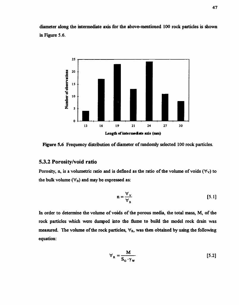
diametex dong the mtermediate axis for the abovementioned 100 rock particles is shown
m Figure 5.6.
13 16 19 2 1 24 27 3 O
t o g t h dinterdrtte axis (mn)
Figure 5.6 Frequmcy distriIlution of diameter of randomly selected 100 rock particles.
5.3.2 Porosityivoid ratio
Porosity, n, is a vohunetric ratio and is defined as the ratio of the vohme of voids (Vv) to
the bulk vohme (!le) and may be expressed as:
In order to determine the volume of voids of the porous media, the total mass, M, of the
rock particles which were dumped mto the fhune to build the mode1 rock drain was
measured. The vohime of the rock paxticles, VR, was then obtahed by using the following
equation:
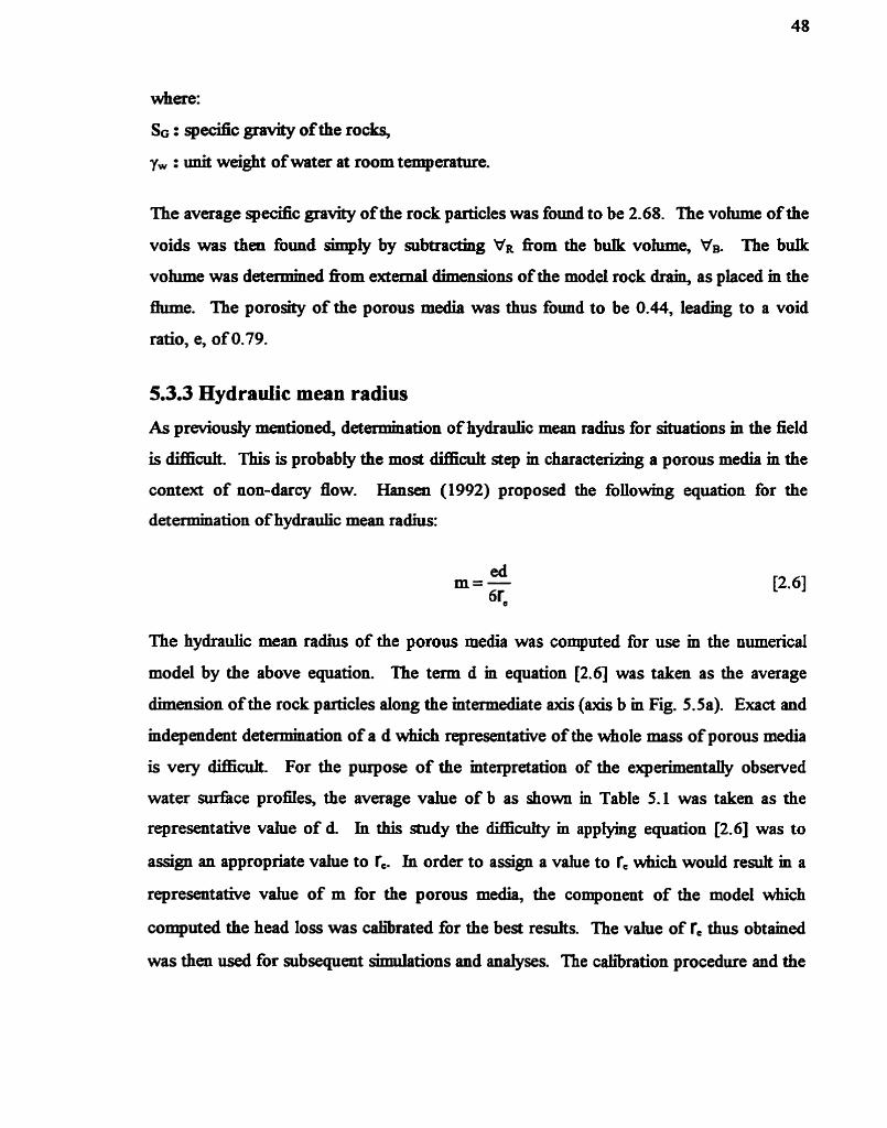
where:
SG : s p d c grevisr of the rocks,
y, : imit weight of water at room temperature.
The average specinc graviry of the rock particles was found to be 2.68. The vohune of the
voids was then found sbply by subtracting VR fiom the buIk vohune, VB. The bulk
vohune was detemineci fiom extenial dimensions of the model rock drain, as placed m the
fhme. The porogly of the porous media was thus found to be 0.44, leadmg to a void
ratio, e, of 0.79.
5.3.3 Hydrauüc mean radius
As previously mentioned, determination of hydraulic mean radius for situations in the field
is àif£ïcuh. This is probably the most düEcult step m characterizing a porous media m the
context of non-darcy flow. Hansen (1992) proposed the following equation for the
determination of hydraulic mean radius:
e hydraulic mean radius of the porous media wa .s computed for use in the numerical
model by the above equation. The term d in eqpation [2.6] was taken as the average
dimension of the rock particles along the intermediate axis (axk b in Fig. 5.5a). Exact and
independent determination of a d which representative of the whole mass of porous media
is very diEicult. For the purpose of the mterpretation of the eqerimentaily observed
water sudace profiles, the average vahie of b as shown Ei Table 5.1 was taken as the
representative value of d In this study the dif l t idty m appiyhg equation 12.61 was to
assign an appropriate vahie to Te. In order to assign a vaiue to Te which would result in a
representative vahie of m for the porous media, the cornponent of the model which
computed the head loss was caharated for the best resuits. The vahie of T. thus obtained
was then used for subsequent simulations and analyses. The calibration procedure and the

r e d s of the cah'bration for optmiized model parameters are outlined in the fonowing
Sections.
5.4 Calibration of Mode1 Parameters
Provision was made m the model to employ either the Wilkms or Stephenson eqyation as
the head l o s equation. The performance of the numerical model in computing water
mfhce profiles when ushg Wïkins' equation as a fiction dope equation was fomd to
depend maialy on values of hydrautic mean radius, m, and porosity, n, such that these
represented the whole porous media. The value of m for a field-scale rock drain c a . be
determineci with a reasonable degree of accuracy since the void ratio, e, and the particle
diameter, d, m the equation which delines hydraulic mean radius (eqp. 2.6) are measurable
and the surface area efnciency, Te, of particles can be estimateci. The performance of
Stephenson equation is maidy dependent on K< (Stephenson's friction factor) and n. The
recommended vahies of for different particles as provided by Stephenson are reported
m Section 2.2.3. Since Stephenson's recommended value for rock (K, = 4) gave computed
water surface profiles *ch were m poor agreement with the experimentally obsewed
water smfàce profiles, it was decided to also sniply calirate the model so as to obtain the
best vahie for the media used.
5.4.1 Determination of parücle surface area efficiency
Non-Darcy flow adaptations of the SSM model were calibrated to get an optimum vahie
of the particle surfàce area efficiency, re. The vaiue of Te thus obtained was used m the
numaical model to determine the m Water çurface pronles through the model rock drain
for mirent discharges were recorded. Water surface profiles were then smnilated for the
experimental discharges by the numerical model, but varying fe and keepmg ail other
model parameters constant. Obsened and Smulated depths dong the porous dike were
then compared, The value of Te which gave the minimum sum of squared error, SSE, was
considered to be the best Te. The SSE was computed using the followhg relationship:

P 2
SSE = x(yib - YL) Pl
where:
j : observed depth of fiow at section j, Y 0,
J : gmulated depth of flow at section j, Ylim
P : total n d e r of sections.
The r e d s of the calibration for Tc are shown in Figure 5.7 and Table 5.2. As c m be seen,
the range of vahies of Te for difFerent discharges for which SSE was found to be mmmnim
was 1.0 - 1.2. The mean value of the optnmzed Tc was found to be 1.10 with a standard
deviation of 0.08 and coefficient of variation of 7.42%.
5.4.2 Determination of Stephenson's friction factor
In a Smilar manxter, the vahie of K, which produced the shdated water d c e profile
with the lowest SSE was determined. Figure 5.8 and Table 5.2 show the results of the
calibration of K. It cm be seen that the range of vahies of K, for which SSE was found to
be minimum was 2.90 to 3.50, and the mean v h e of K, was found to be 3.10 with a
standard deviation of 0.25 and coefficient of variation of 8.12%.
5.4.3 Comments on the values of r. and K,
As stated in Section 5.4.1, the vahies of the relative surface area efnciency, Tc, found m
this study range fkom 1.00 to 1.20. An average value of 1.10 was taken as the
representative value for f, Similatiy, the range of Stephenson's fiction fàctor, K, was
found to be 2.90 to 3.50 and an average value of 3.10 was taken as the optimum value to
use subsequently m predictive purpose.

0.00 0.40 0.80 1.20 1 .BO 2M
Surface area dficiency, r.
Fiure 5.7 ûptnm;llltion of surface area efficiency, Tep in the Wilkins equation.
1 .O0 200 3.00 4.00 5.00 6.00
Stephenson friction factor, K(
Figure 5.8 Opthkation of fiction fàctor, &, m the Stephenson w t i o n .

Table 5.2 Resuhs of the catibraticm for the optimum mode1 parameters.
Discharge Surfiicearea Stephenson's
Cu@ &ciency, re fiction faaor, K<
O. 70 1.20 3.50
The term Tc represents the extent to which a particle differs in shape and roughness fiom a
smooth and pdect sphere. For snooth and perféct spheres the value of Te is 1. A
cornparison among the vahes of r. of the porous media used by Wilkms (1956), Hansen
(1992), and that used in this shidy can be made. Such a cornparison is shown m Table 5.3.
The vahes of r, for the porous media used by WiIkins (1956) was calculated and
presented by Hansen (1992) based on published data. Vahies of Te for the porous media
used by Hansen (1992) was determined by a d experiment. Wilkms (1956) used
cnished dolente as the porous media. On the other hand, c d e d bes tone was used as
the porous media m the present study and also m the study pdormed by Hansen (1992).
It can be seen fiom Table 5.3 that, compared to the vahies of fc for similar sized particies
used in other studies, the vahie of rc m this study is lower and is close to the vahe for
spheres.
Stephenson (1979) has siated that the value of friction factor, K, approaches 1 for smooth
spherical marbles, is about 2 for semi-rounded gravels, and is about 4 for sharp cnished
Stones. In detefDninjLlg the abovementioned values of K, Stephawn used data fiom a
number of similar studies. The authors of some of these studies did not publish ail the
associatecl numerical data. Under such circumstances Stephenson used reasonable

assumptions and performed his malpis based on these assumptions. 'Lhe vahies of Kt thus
found wexe pomts on hes fïtted through scattaed data* The scatter in the data was wide,
and the vahes of Ki varied fiom about 1 to about 11, for differerit types of porous media.
The average optimum vdue of K< = 3.10 found in this shidy, therefore, cm be considered
as reasonably close to the recommended value of Kt = 4 for an+ c d e d rock by
Stephenson (1979).
Table 5.3 Cornparison of particle surfàce area efnciencies*
'Ihe fonowing points should be noted regardmg the procedure followed m this study to
determine the optmnun vahes of the parameters f. and K:
The optimum vahes of Te and K, were determkd by nhhnhbg the SSE (@en by
eqn 5.3). In minimi7mg the SSE for a @en discharge, the observed water levels were
rewrded at number of cross-sections of the model rock drain- The numerical model
deveioped m Section 4.2 was then used to sinnilate the profile for a given discharge
The values of T, or Kt which resuhed in the mmimiim SSE were considered as the
optimum vahies. The observed profiles were recorded dong the entire longitudinal
section of the model rock drain. Compared to open channel flow, the streamhes of
the non-Darcy flow through the model rock drain were fàirly steep, especialy near the
exit of the drain. The flow was therefore somewhat 2-D in nature near the exit fice.

This experimental departme fiom GVF theory (near the exit fice) introduced some
error in the ïe found by the optimization procedure.
The representative particle diameter used in this study was based on the meamernent
of 100 randomly selected puticles The pamcle diameter thus calculated was no
doubt dightiy different fiom the liiameta t d y representative of the entire porous
media.
The porosity was calnilated fiom the vohmetric ratios found fiom physical
measufement, This mchided measurement of the bu& volume of the mode1 rock drain
(wiîh a somewhat iIl-defïned uppa surfàce), the average specinc grevity of the
particles (subject to the same question of representativeness as raiseci m pomt 2), and
the mass of rock piaced m the fiume. Aithough the resultmg computed porogty was
reasonable, there m y have been imknown systematic mors m hdmg n. There may
also have been local variations m the porosity within the mode1 rock drain.
Both W W s (1956) and Hansen (1992) attempted to mdependently estimate m by
experimentaIly trymg to find representative surface areas of the particles used m their
studies. Deparhues of the true m values for the porous media used in the cohumi tests
would then have been absorbed by the W factor, m the case of Wiikms' equation
(Hansen (1992) did not propose y& another non-Darcy flow eqyation). Independent
(geometrically-based) estimates of Te based on particle surnice area estimates generally
assume disc-like and bladelike particles in the porous media do not cause a significant
amount of particle area to be lost to inter-particle contact (Hansen, 1 992). As can be
seen nom the Zingg diagram (Figure 5.5 b) prepared for the porous media used m uIls
study, a sipificant portion of the sample rock fen m the category of disks.
The diffaences between the vahies of the T, and Kt found m this study and those obtained
m Smilar studies (ie. Willrins, 1952; Hansen, 1992; Stephenson, 1979) may be due to any
one or a combination of the above-mentioned reasons.

5.5 Depth of Fiow at the Emergent Face
For a &en discliarge, the steady state non-Darcy water sudice profile through a
psrticular rock drain wiiî foîiow an eqdiirium shape dependmg on the characteristics of
the media and fiuid This profile through rock drain can be computed wing the mode1
developed m Section 4.2, starting nom a known wata leveL For the SSM this starting
elevation is at the downstream 1Bna, for subcntcal flows, and at the apstream b i t , for
supercritical flows Superdcal Bow rarely occurs m flow through coarse porous media,
so that the startmg section is usually at the downstream linnt of the rock drain. It is
therefore necessary to have knowledge about the depth of flow at the emergent &ce, also
caIIed the "exii depth', m order for the SSM to commence flow profile computations.
For tme open chanael flow (no porous media), the theoreticai depth at a brink may be
computed for a rectanguiar channel as:
where:
y= : critical depth,
q : unit width flow rate.
Due to the curvature of the streamhes of open channel flow near a bri& Ït is known that
the critical depth actuaily occurs 3 to 4 h e s y=, upstream of the brink (Rouse, 1946).
For a fùlly-developed turbulent flow through coarse porous media the exit depth can also
be assumed to be equal to the Çritical depth, the depth at which the specific energy is
mmimiim (Stephenson, 1979). The criticai depth for non-Darcy flow can be derived by
differatiating the energy equation in the same manner as is done for open channe1 flow
(Chow, 1959). The specinc energy, E, at the downstream section of a rock drain cm be
defhed as:

Differentiating eqyition [5.5] with respect to depth of flow, y, and setting dUdy equd to
zero for minimiim specinc energy yields:
Substitution of - for UV yields: n-A
Applying assu~lfptions o f a = 1.00, and CO& = 1.00 mto equation 15.7 yields:
Therefore at critical depth for non-Darcy flows, the pore Froude no, h p is eqyal to one.
For a @en discharge and channel cross-sections, the cntical depth can be searched for by
vaiymg the magnitude of y. The vahie of y which r e d s m = 1 is the critical depth.
For rectangular channets the critical depth, y=, can be computed directly by:
[S. 101
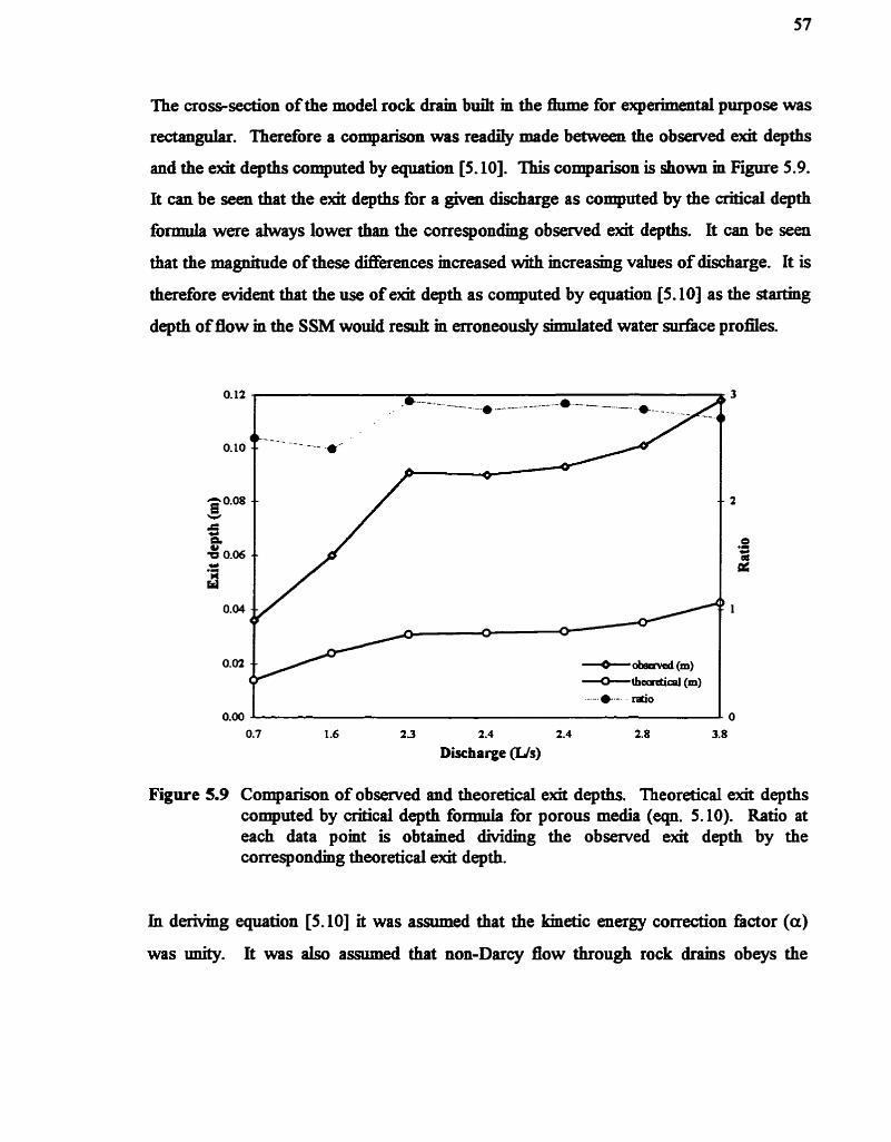
The cross-section of the mode1 rock drain b d m the fhme for experimental purpose was
rectanguiar. Therefiore a comprison was readïly made between the observed exit depths
and the exit depths computed by equation [5.10]. This comparison is shown in Figure 5.9.
It can be seai that the exit depths for a given discharge as wmputed by the d c a l depth
formiila were always lower than the corresponding observed exit depths. It can be seen
that the magnitude of these differences mcreased with increashg vahies of discharge. It is
therefore wident that the use of exit depth as computed by equation [S. 101 as the starhg
depth of flow m the SSM would r e d m ezroneously simulated water surface profiles.
.- -. *.-. do
0.00 O 0.7 1.6 23 2.4 2.4 2.8 3.8
Discharge (Lh)
Figure 5.9 Cornparison of observed and theoretical exit depths. Theoreticai exit depths coquted by critical depth formula for porous media (ecpi. 5.10). Ratio at each data pomt is obtained dividing the observed exit depth by the correspondmg theoretical exiî depth.
In derivmg eqyation [S. 101 it was assumed that the kinaic energy correction fàctor (a)
was It was also assumed that non-Darcy flow through rock drains obeys the

assumptions of GVF theory normdly applied to open chamiels. GVF theory is based on
the assumption that the flow is horizontal In &ct, for the non-Darcy %ow through model
rock drain the streamlines are faHiy steep, near the exiî ( d o g o u s to behg near the brink
m open chatmel flow). 'This breakdown of a key assimiption of GVF is thought to be the
main reason for the discrepancies seen m Figure 5.9.
The ratios of observed exit depth and the exit depth computed by equation 15.101 for
various discharges through the model rock drain are show in Figure 5.9 and Table 5.4.
The mean of these ratios was found to be 2.8 wah a standard deviation of 0.17. Ahhough
there may be some mors m determinhg observed exit depth (due to tuhulaice), it can be
seen that the percentage deviations of the ratios f?om their mean is dways les than 10.
These d deviations of the ratio of the observed exit depth to the exit depth computed
by equation [5.10] fiom the mean suggest a simple linear relationship of the foflowhg
form for the model rock drain between the a d (obmed) and theoretical exit depths:
Table 5.4 Ratio of observed and theoretical exit depths.
Discharge
O 0.70
1.60
2.33
2.39
2.44
2.84
3.75
C6mm aquatioi
Exit depths
Observed, Y*4 O
3.6
6.0
9.1
9.0
9.3
10.1
11.8
[S. IO]
Ratio Percentage deviations of ratios fiom the mean**
-7.0
**mean ratio = 280

When th- is d c i e n t data for a field-scale rock drain, a simple stagedischarge
relation&@ can be developed for the mergent fice. Ifthe exit depth wmputed by such a
stage-discharge equation is higher than the exit depth as computed by equation [S. 101, the
higher depth should be used as the exit depth. Otherwise, computation of the water
suxfàce profile should commence at critical depth because the depth of flow can never be
l e s than the critical depth for subcritical flow. For cases where there is no data on which
a stage4kcharge curve may be based, computations miist start fcom the critical depth.
Ahhough a constant ratio between the observed and theoretical exit depths probabS,
e&s, and the theoretical exÏt depth can be adjusted by this ratio to give the analyst a
better startmg point, the applicabiiay of eqyation 15.111 is not known for slopmg
dowwtream nices. In any situation when wing critical depth as the s t h g depth in water
mfàce profile computation, it is necessary to use very d finite dineremce spacing m the
numericd scherne for the SSM. This is because at or near the d c a l depth the pore
Froude number, kp, is close to or equal to one and there is an inverse dependence
between Ffp and grid spachg. Detaiis on the numerical effect of grid spacing are
discussed in Sections 7.2.3 and 7.2.4.
The depth-discharge relations&$ at the emergent face of the mode1 rock drain was
developed fiom a power law regression as:
The performance of equation 15.121 is shown in Figure 5.10. If there is data, a depth-
discharge equation like the one presented above is veq useM m water surfàce profile
computation for a field-scale rock drain. Necessary care should be taken to ensure that ail
data used in developing such depth-discharge curves for a field-scale rock drain
correspond to a drain of k e d length because the coefficient and exponent in the power

1 .O0
Discharge (L/s)
Figure 5.10 Depth-discharge curve for the model rock drain at the emergent fice.
iaw equation might change if the drain length changes, resuhsig in the diffèrent exit depth
for the same discharge. This f k t makes the development of depth-discharge c w e s for a
field-scale rock drain a diflicult task because the rock drains are formed fiom the by-
products of a contmuous mining operation, and the length mcreases with tirne.
5.6 Cornparison of Simulated and Obsewed Water Surface Profiles
Due to the fàct that the field data were unavaüable, the performance of the model was
evahiated by comparing model output to the data generated f?om the experiments
pedonned on the model rock drain. The eqerimental setup and procedure, description of
the porous media used in the experiments, and the determination of optimum values of
various parmeterç in the non-Darcy flow equations were described iu precedmg sections.
As the nrst step of the evaluatitm of the model pedo~lltlllce, water surface profiles were
recorded fiom the glas wdl of the h e where the model rock drain was buih. At the

beghnhg of each nm, the speed of the pump and the water level m the h were
adjusted to obtain the desired flow rate, which was then recorded. Once steady state
conditions were achiwed, the depths of water dong the model rock drain were recorded.
In this way the water surfàce pronles were recorded for discharges of 0.70 Us, 1.60 Us,
2.33 Us, 2.39 Us, 2.44 Us, 2.84 Us, and 3.75 U s From these observed water sdbce
profiles, the data rehting to discharges 0.70 Us, 2.33 Us, 2.44 Us, and 2.84 Us were
used m the calibration process for optmiuiing non-Darcy fiow eqytion parameters and the
remaining data (for the discharges of 1.60 Us, 2.39 Ys, and 3.75 Us) were used for
evahmting the performance of the modeL In orda to evaiuate the performance of the
model, water surnice profiles were simdated for the model rock drain for discharges of
1.60 Us, 2.39 Ws, and 3.75 L/s and compared with the observai water d c e profiles.
In smnilating the water surface profïies, the depth of fiow at the starting croçs-section (the
initial depth) was ahvays taken fiom the obçerved data. The results of these simulations
and cornparisons for discharges are presented in Figures 5.1 1 and 5.12. Figure 5. L 1
presents the outcomes when the model used Wilkins' equation to compute the fiiction
dope, and Figure 5.12 presents the outcomes when the Stephenson equation was used. In
these cases the water surfàce profiles were simuiated ushg a scheme smiilar to SSM in
GVF. The headloss between any pair of sections was computed fiom the anthmetic
average of the fiiction dopes of neighborïng sections. In Snnilating water surface profiles
using the Wilkins equstion (Figure 5.1 l), the optimal shape coefficient (Te) of 1.10 was
used Sindarly, the optjmai fiction factor 6) of 3.10 was wd in Snnilating the water
surfàce profiles using the Stephenson equation (Figure 5.12). The SSE's of the water
surface pronles for various discharges are reported in Table 5.5. It cm be seen ftom
Figures S. 11 & 5.12 and fiom Table 5.5 that the performance of the model in simdating
water sudice profïies is qyite sati.cfactory. The minor deviation of the shdated water
d c e profiles fiom the observed water Surface profiles may be due to miperfect
cbaracterization of the porous media. In this study, in characterizhg the porous media
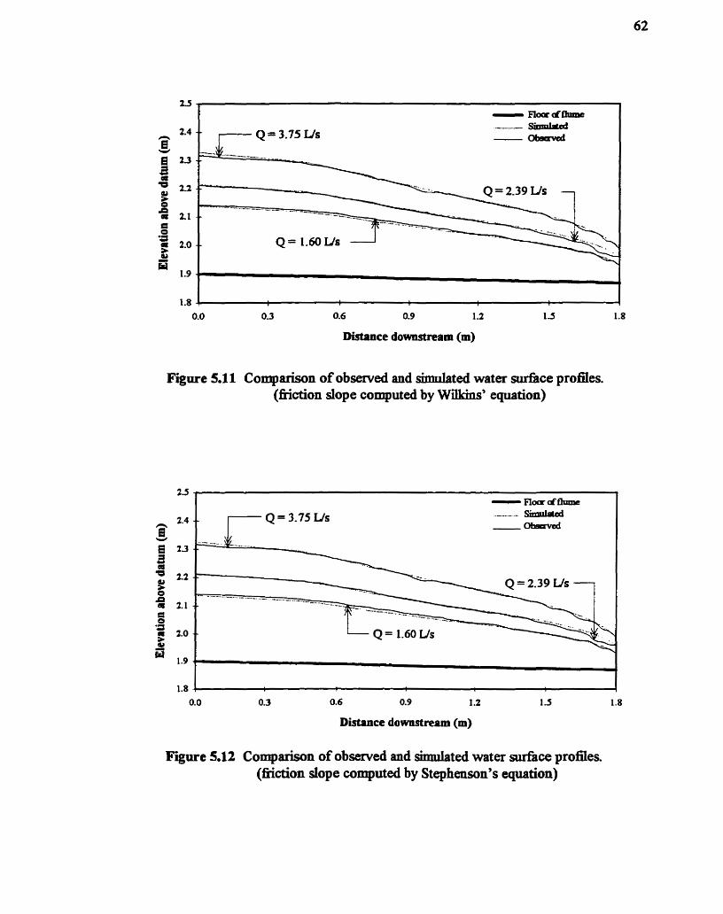
D i c e downstream (m)
Figure 5.11 Cornparison of obsened and Snniiated water sdàce profiles. (fiction slope computed by Wiikins' equation)
0. O 0 3 0.6 0.9 1.2
Distance downstream (m)
F i e 5.12 Cornparison of observecl and ssmilated water surfàce profiles. (fiction slope computed by Stephenson's equation)

Table 5.5 Differences between obsaved and simailatecl water d c e promes.
various parameters releting to non-Darcy flow equations nameiy, d, e, Te, and % were
measured or mferred. Systematic error m e and d was wmpensated for hding the Te
which gave the best overall match, but this would not have compensated for local
variations in these three parameters. The same is tme of K, It can be seen âom Figures
5.11 and 5.12 that there are some local mdulations m the observed water sudice profiles,
especdly near the downstream face. The observed water suditce profiles were recorded
fiom the coordinate grid drawn m the glas wall of the fiume. hiring the experiments
water tended to preferentiaiiy flow between the glas walls of the fiuxne and the Stone. No
linmg was used in the fhme to compensate this wall-effect, which was probably smaIL
A h , for the non-Darcy flows deah with here, the niction dope was Sgdicant, especiany
near the downstream face. Occasional mterpolation of the observed wata surface profiles
during the recordhg may be the cause of some of the undulations in the observed water
surface profiles. The flow at the exit is also more 2-D m nahue, and this may have
promoted undulations near the dow~l~tream face. It cm also be readily seen fiom Figures
5.11 & 5.12 and Table 5.5 that both the Wilkins and Stephenson equations Smulated
similar water surfkce profiles for the three different discharges. The SSEYs for the
discharge of 1.60 Us were foimd to be 0.0009 m2 and 0.0013 m2 for Wilkms and

Stephenson equatim respectiveiy. The SSE's for the other two discharges (2.39 Us and
3.75 Us) w a e computed as 0.0016 m2 and 0.0008 m2 when WiiLms' equition was use4
and 0.0016 m2 and 0.0007 m2 when Stephenson's equation was used. It cm therefore be
concludeci that the Wdkins and Stephenson equations perfonned equanY wen m simdating
the eqerimental water surâice profiles through the model rock drain.
5.6.1 Effect of friction dope caiculation method on fîow profile
In coqutmg the head loss, &, between any pair of d o n s under the SSM procedure,
the distance between the sections, Ax, is mdtiplied by the representative friction slope,
sfnP , for the reach bounded by the two sections (eqa 4.3). One Smple way to define the
representative fiction slope between a pair of sections is the anthnietic average of the two
sections (eqn. 4.4). There are a number of other methods available in the Iiterature for
estmiating the representative fiction dope for GVF. Two 0 t h wideiy used methods of
estnnating representative fiction slope are the geometric mean and the hmnonic mean.
The geometric mean and the harmonic mean fiction dope models for a pair of sections
can be defined by
(geometric)
(harmonic)
HEC-2 (Feldman, 1981), the popuIar water suditce profile compation model, uses the
geometïic mean of the fiction dope for MZ profiles. Reed and WolfkiU (1976) also
recommend the geometric mean fiction dope mode1 for Sniüat flow profiles Tavener
(1973) recommends the harmonic mean fiction slope model for M2 profiles. Ail such
reconnnendations regcudiug the fiction dope model are based on the r ed t s of studies on
GVF m open channek. There appears to be little or no idormation m the literature
regardmg the relative suitability of these averaging procedures m water sudiace profile

computation for non-Darcy flows. In order to evahmte the performance of the mode1
developed m this shidy m smnifating water surface profiles for the three different fiction
slope averaging techniqyes mentimed abwe, profiles were smnilated ushg the different
fiiction slope models. The SSE's were computed for these water surfice profiles and are
reported in Table 5.5. It can be seen Born Table 5.5 that dl the fiction slope modek
pdorrned weIL m simiilatmg the water surfàce profiles, m that the SSE's are almost the
same- Resuhs show that, for the discharge of 1.60 Us, the arihnetic mean performed
the best. For the discharges of 2.39 Us and 3.75 Us, the performance of harmonic mean
was the best. Based on the resuhs presented on Table 5.5, it can be concfuded that any of
the above-rnentioned fiidon slope averaging techniques wiil produce satisfaaory
estimates of flow through rock drains, provided reach Iaigths are not excessive. At this
stage Ït is f i c u l t to recommmd a specific nveraging technique for a specific type of flow
profile for field-sale rock drains because there is a severe shortage of data on which to
base such conchisions.
5.6.2 Effect of level of turbulence on the flow profiie
In most cases, the flow through field-sale rock drains is fiiny turbulent. The Reynolds
number for such rUny-deveioped turbulent non-Darcy flows through rock d e may be as
high as 10'. It is recoghxl that the exponent of the velocity temi in the equations
descri'bing flow through porous media is unity for laminar flow m a fine medium (ie.,
following Darcy's law, eqn. 2.1). This exponent mcreases as the Re mcreaseq and
approaches 2 for fully-developed turbulent flow, as in the Stephenson equation (eqn 2.10).
ûther than the Stephenson e~uation, most non-Darcy flow equations are based on
experiments with Re vahies less than 104, and m very few cases have iaboratory
expiments been supplemented by m-Shi field measurements. Such vahies of Re are
significantiy lower than what actuaily occurs m natinal rock drains or buried çtreams The
experiments which are based on low Re tests ofken result m equations having the exponent
of the velocity term less than 2. The Wilkins equation shows head loss being proportional

to ul-" (eqn. 2.4). 'ïhe exponent on U m the Wilkms equation mdicates that the equation
describes the regmie of a non-Darcy flow m the n e fùIly-developed turbulent flow
range. On the other hd, the Stephenson equation was developed on e>cperHnents based
on large Re (Re > 10'). Stephenson (1979) obtimed vdocities as hi& as 0.5 dsec irt his
experiment by using f idy large rocks (d = 0.1 5 m).
The range of Reynolds nambers in the eqeriments conmict ed m this study are reported m
Table 5.6. It can be seen fiom Table 5.6 that when the Re vahie is low, the SSE
associated with Wilkins' equation is d e r than that associated wiîh Stephenson
equation As the Re vahie increases, the SSE's associated with WdkW equation becorne
higha than those asociated with Stephaison eguation. Although the shortage of field
data precludes reachmg any definitive conclusions regardmg the comparative performance
of the Wilkms and Stephenson eqyations m predicting water surnice profiles through rock
drains, it is expected that the Stephenson equation would perform betta under fùüy-
developed turbulent flow conditions, Le., for non-Darcy flow through field-seale rock
drains.
Table 5.6 Reynolds number for different discharges.
Range of
Reynolds numbe~
SSE ( 104 mz) wmns' equation
Stephenson's
equation

5.6.3 Effect of cross-sectional variability in flow profile
As previously mentioned, to Smiilate to some degree the na- conditions of a rock
drain, the width of the model rock drain was varied by hstalling wooden planks m the
thune. The crosssections of the model rock drain along the iength of the fhme are shown
in Figure 5.1. The simulated and observed water surface profiles through the model rock
drain have been shown in Figures 5.11 and 5.12. h this aspect of the work an effort was
made to mvestigate the behavior of non-Darcy flow profiles through non-prismatic
channels and quanti@ the response of same for such conditions.
Temporary constrictions generally cause temporary depressions m the water surface
profile, as long as the conmiction is not too swere. The reason for this phenornenon, and
the limit on the magnitude of the constriction which will not cause a backwater effect
upstream of the constriction, may be found nom the specinc energy diagram (see Figure
5.13).
The response of water surfàce to cross-sectional variability of a hypothetical horizontal
open chamel is shown m Figure 5.14. Although Figure 5.14 is a qualitative diagram
d r a w for open channeis having rectangular cross-sections, for other g e o m d c shapes or
naturd cross-sections, the behavior would be mnilar. Because of the fact that the flow
through bwied streams behaves simrlariy, to some extent, to that of open channels, a
similar response might be expected for non-Darcy flow through rock clraius for the same
geometric changes. It can be seen fiom Figures 5.11 and 5.12 that the experimentally
observed response of the non-Darcy water surface profiles to such cross-sectional
variation was not obvioudy simiiar to that of open channel flow profiles. This Merence
m behavior of non-Darcy flow profiles fkom those of GVF can be explained with the aid of
the energy equation, equation [4.2].
The plan of the width of the model rock drain along the f h e is shown m Figure 5.15.
The locations where the drain width abnrptly changed is represented m the figure by
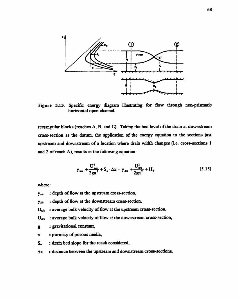
F i e 5.13. Specinc en- diagram iliwtrating for flow through non-prismatic horizontal open chamel
rectanguiar blocks (reaches 4 B, and C). Taking the bed level of the drain at downstream
cross-section as the datum, the application of the energy equation to the sections jusr
upstream and dowmtream of a location where drain width changes (ie. cross-sections 1
and 2 of reach A), rernilts m the followhg equation:
where:
y ~ . : depth of flow at the upstream cross-section,
ya, : depth of fiow at the dowmtream cross-section,
Uds : average bu& velocity of flow at the apstream cros+section,
Udh : average bulk velocity of flow at the dow~~sbleam cross-section,
g :gravitatiOnalCOI1StilI1t,
n :porosityofporousmedia,
S, : drain bed dope for the reach congdered,
Ax : distance between the upstream and dowwtream cross-sections,
[S. 151

(a) Plan
(b) Elevation
Figure 5.14 Qualitative response of water surface profile to changes m chuuiel width for a rectangular open channel with no porous media (for sub critical flows).

Figure 5.15 Change of width of the mode1 rock drain dong the Bume. (plan view, all dimensions m mm)
& : head loss between upstream and downstream crosîsections due to fiction.
After remangement, equation [S. 1 51 becomes:
in the above equation Substitution of Ay for (y, - y,,l) and Ahu for
yields:
The t e m Ay in equation [S. 17 represents the drop or rise m the depth of flow fiom the
upstream to the downstream cross-section. A positive value of Ay represents a drop in the
depth of flow and a negative vahie represents a rise m the depth of flow, in the direction of
flow. The term labeled 1 m equation [5.17l represents the head loss or gain due to the

change m the velocity head ( resubg fiom change m cross-sectional area fiom upstream
to downstream), the term II represents change m head caused by the gradual and unifom
decrease in the elevation of the bed (for descending dopes), and the temu III represents the
head loss due to fiction.. The Sgn of t e m II m equation [5.171 is positive for the case of
an ascendhg dope. Unless energy is added to the system, the term III in equation (5.17j
is ahvays positive. At the transition zone where width of the chamel abniptly changes,
such as the reach between cross-sections 1 and 2, the head losses due to change m velocity
head and due to friction also abrupt. At other locations, such as the reach between cross-
sections 2 and 3, where the width is constant, they are graduaL At al1 locations m a given
reach the change m head caused by the d o m decrease m the elevation of the bed is
considered gradual
If a cornparison is made between the Figures 5.14 and 5.15, a rise m depth of flow might
be expected m reach B (âom cross-section 3 to 4) because the flow experiences an abrupt
expansion. Such a rise can also be expected m reach C, between cross-section 5 and 6.
However, a rise in water level was not observed m those locations of model rock drain
(see Figures 5.1 1 and 5.12). This behavior cm be explained by using the equation [5.171.
The vruious terms of equation [5.173 in reaches 4 B, and C for water niraice profiles
through model rock drain for various discharges are tabulated m Table 5.7. It can be seen
fiom Table 5.7 that for the discharge of 1.60 Us, the signs of the term Ahu (i e., term 1 m
eqn. 5.17) m reaches B and C are negative. This mdicates a gain m head at those two
locations due to the change m velocity from upstream to downstream These gains m
head m reaches B and C are 0.13 mm and 0.08 mm, respectively. At the same time, the
loss of head at the same locations due to fktion are 4.20 mm and 6.7 1 mm, respectively.
These vahies, when put m equation [5.171, result m a total loss m head (denoted by Ay in
eqn. 5.17) m reaches B and C of 3.36 mm and 5.58 mm, respectively. Simüar losses m
head were observed for other discharges at the same locations. The velocity through the
rock drain is significantly smaIl compared to that through the open channels. This hct

Table 5.7 Computation for 105s or rise in head
Feature Reach A Reach B Reach C

results in the magnitude of the term 1 m equation [S. 17J behg a very srnaIi quantity
compared to the other two terms (see Table 5.7). In almost an Stuations, no matter how
severe the constriction is (unless it is close to the critical condition) this d value of the
term 1 has a minor effect on the calculation for rise or loss m depth, Le. in equation [S. 17J.
The head loss due to fiction (tem III) for non-Darcy flow is so high that În aimost an
situations the combined magnitude of the terms 1 and II c m be expected to be lower than
that of term ID. This leads to the fbct that m almost ail cases the depth of flow at any
cross-section for a non-Darcy flow is lower tha. that of the next-most upstream cross-
section. For a &en discharge, the flow experienced total loss m heads (Ay) at all
locations of mterest (ie., in reaches A, B, and C). Ahhough the losses of heads were
abrupt, abrupt drops m water surfàce profiles were not observed at those locations (see
Figure 5.1 1 and 5.12). Water surnice profiles plotted in Figures 5.1 1 and 5.12 reflect the
fàct that the drops reported in Table 5.7 were s n d However, distinct and gradual water
surfàce dopes can be observed for the reaches between upstream and reach 4 between
reach A and reach B, between reach B and reach C, and between reach C and the
downstream Limit of the rock drain.
5.7 Application of the Model to a Typical Prototype Rock Drain
The model developed m Section 4.2 is theoreticaily capable of simulahg water surface
profiles through any natural rock drain. The performance of the model m c;imulating water
d c e profile under laboratory experimentai conditions was fomd to be satisfàctory.
Data unavailabüity preciuded amving at smiilar conclusions regardmg the performance of
the model m water h c e profile sindation mder naturai conditions. In order to see
how the model works mder natural condition, water 6 c e profiles were simulated based
on hypothetical information. This mformation was carefùily chosen so that it represented
a typical prototype rock drain. The assumai data is a rough approximation of the Lme
Creek drain located m the Kootenay mountains, south eastem British Cohunbia.
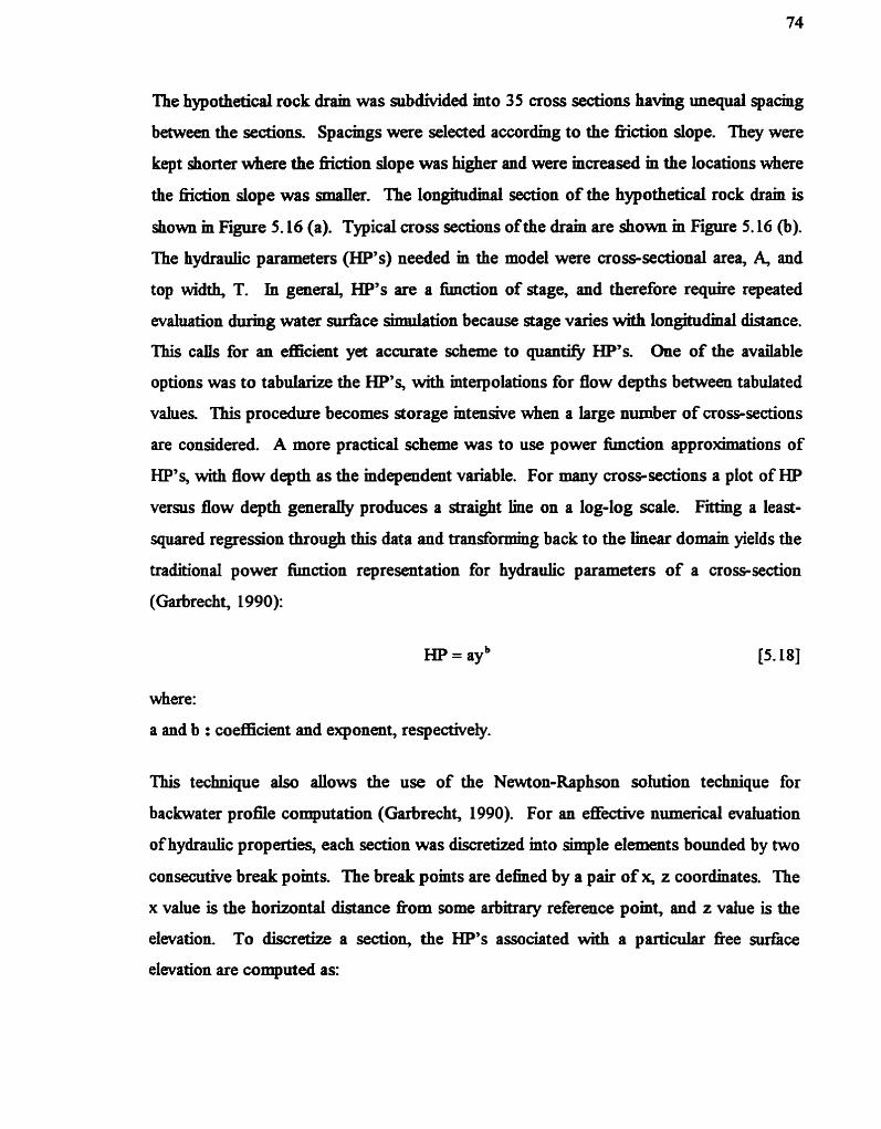
The hypothetical rock drain was subdivided hto 35 cross sections having unequal spacing
between the sections Spacings were selected accordhg to the fiction dope. They were
kept shorter where the fiction dope was higher and were mcreased in the locations where
the fiiction dope was smaIIer. The longitudinal section of the hypothetical rock drain is
shown in Figure 5.16 (a). Typical cross sections of the drain are shown in Figure 5.16 @).
The hydraulic parameters (HP's) needed in the mode1 were cross-sectional area, A, and
top width, T. In general, HP's are a hction of stage, and therefore require repeated
evahution during water surface sindation because stage varies with longitudinal distance.
This calls for an efficient ya accurate scheme to quant@ HP's. One of the avaüable
options was to tabuhize the HP's, with mterpolations for flow depths between tabulated
values. This procedure becomes storage intensive &en a large number of cross-sections
are considered. A more practical scheme was to use power hc t ion approximations of
HP's, with flow depth as the mdependent variable. For m a . cross-sections a plot of HP
versus flow depth generally produces a straight line on a log-log scale. FatSg a least-
squared regession through this data and transfoRning back to the linear domain yields the
traditional power fimction representation for hydraulic parameters of a cross-section
(Garbrecht, 1990):
where:
a and b : coefficient and exponent, respective@.
This technique also dows the use of the Newton-Raphson sohition technique for
backwater profile computation (Garbrecht, 1990). For an effective numerical evahiation
of hydraulic properties, each section was discretized mto simple elernents bounded by two
consecutive break pomts. The break pomts are dehed by a pair of x, z coordinates. The
x value is the horizontal distance fiom çome arbitrary reference pomt, and z value is the
elevation. To discretize a section, the HP's associated wah a particular fiee surface
elwation are computed as:


where:
j : section element cornter,
NS : the n d e r of section elements at or below the fiee water surfàce.
Data relathg to the values of the HP's were generated using equations [5.19] and [5.20]
with a 1 m mtervai in the z direction. This was subsequentiy used to derive equations such
as [5.18] for requisite hydraulic parameters (A and T) for each cross-section.
The açsumed vahie of d the other mode1 parameters are reported m Table 5.8.
Simulation of water surfàce profiles was performed using the hypotheticd data as shown
m Table 5.8 for discharges of 70.0 m3/sec and 85.0 m3/sec. Sindations were performed
using Wilkins' equations as the head loss equation. The results of these simillations are
shown m Figure 5.17.
Cross-sections of the hypothetical rock dram were varied mtentionally so as to simulate
the natural variation of the field-scale rock drain (see Figure 5.16) and also to mvestigate
the effect of such variations on the water surface profile for a field-scale rock drain. The
water surfàce profiles from 'upstream' to pomt 'b' correspond to cross-section 1 - 1 m
Figure 5.16 (b). Profiles fiom points 'b' to 'c', and nom pomt 'c' to 'downstream'
correspond to crosssections 2 -2 and 3 - 3, respective@. It can be seen fiom Figure 5.17
that the shape of the profles fiom 'upstream' to pomt 'b' is Smilar to an M l profile of
GVF. The shape from pomt 'b' to 'downstream' is Smüar to an M2 profile of GVF. It
can be also seen that water surnice profile d e r pomt 'c' did not recover to the previous

Table 5.8 Assumed value of parameters reliting to hypothetical rock drain.
-
Similar to M1 profile o f W - 1 2 3
\ I
v Q: 70 m'/sec
Similar ta M2
- C r d bad kvel - witu lcvel 1 2 3
600 900
Dijkacs downstream (m)
Figure 5.17 Smnilated water surface profiles through the hypothetical rock drain.
level even though the flow experienced a much wider crosç-section (see Figure 5.17).
These water surface profile variations, especially the latter case, are somewhat Merent
fiom what undly happais in open chameh under sinnlar conditions (see Figure 5.14).
Smiilar behavior was also observed for the non-Darcy profiles through mode1 rock drain,

and the reasons for such behavior were explained in detail with the aid of the energy
equation (ecp 5.17). In a similar âshion, the energy eqyation c a . be used to explain the
behavior of the wata mrfàce profiles observecl for the field-seale hypotheticai rock drain.
The numerical values of all the temis m energy eqyation (eqn. 5.17) for a number of cross-
sections are reported m Table 5.9. By way of discussion and exphmation the flow profile
for the reach 'upstream' to pomt 'b' will be considerd frst. As previody stated, the
shape of the flow profile in the abovementioned reach is smiüar to an Ml profile of GVF.
Consider any two cross-sections at points 'a' and 'b' on this Ml portion of the water
d c e profile through the hypotheticai rock drain (see Figure 5.17). It can be seen nom
Table 5.9 that for the reach 'a' to 'b' term 1 (the headloss due to a change m velocity
head) m the energy equation (eqn. 5.17) is very small and tenn III (the head loss due to
fiction) is also small. Their sum is srnaller than term II (the change m head caused by the
d o m decrease m the elevation of the bed). This results m a negative vahe of Ay which
is indicative of an mcrease m depth m the direction of flow. 'Lhis phenornenon cm be
observed between any pair of sections for the entire reach defhed by 'upstream' to pomt
b ' The depth of water for the reach 'upstream' to 'b" is large and this large depth of
water results m a large flowthrough area, &ch leads to a velocity through the void
spaces of the porous media of the hypothetical rock drain (since the velocity is calculated
by dividing the discharge by fiowthrough area). The 4 void velocity (UV) results m
relatively small Ection dopes because the fiction dope is a function of UV'-" (for
Wilkms' equation) or uv2 (for Stephenson's equation), so that the Sgn of the change m
depth of flow fiom upstream to downstream, Ay, for any pair of sections for the reach
'upstream' to 'b', is negative (set Table 5.9). lhis is the reason why, withsi the reach
'upstream' to 'b', the water surfàce profile foUowed a shape similar to an M l profile of
GVF.
In the reach 'b' to 'c' the cross-section is severeiy wnstricted (see Figures 5.16) r e d t h g
m a large increment m velocity, which results m a large loss due to fiction. This loss due

Table 5.9 Magnitude of various terms of the aiergy equation* of hypothetical rock drain.
Section (a) - (b)
T m 1 (m)
Term II (m)
Tenn III (m)
Term 1 (m)
Tenn II (m)
Term IïI (m)
Section (b) - (c)
Tenn 1 (m)
Term II (m)
Term IiI (m)
Term 1 (m)
Tenn II (m)
Tenn ïïI (m)
-ai [S. 1 1
Section (c) - (d)
Term 1 (m)
Tenn II (m)
Term III (m)
Term 1 (m)
Terrn II (m)
T m III (m)
to fiction is much larger than the change m potential head between points 'b' and 'c'.
This results m the sign of the temi Ay being positive, mdicating a &op m the water nirface
profiles. The numeric vahies of Ay for the reach between 'b' and 'c' is large, and this
large vahie is the reason for the sharp drop m the water surface profiles m reach 'b' to 'c'.
Within the reach between pomt 'd' and 'downstream', the shape of the profile is similar to
an M2 profile of GVF. Afier passing section 'c' the flow experiaiced nnich wider cross-
sections and wuld not recover its depth. This is what uniaiiy happens with the fiee
swfkce pronles of open channels under Smilar conditions. The depth of water at pomt 'c'
is low, which r e d s in the large velocity of flow and which ultimately leads to large loss
of head due to fiction. This head loss is not as large as that within sections 'b' to 'c', but
it is larger than the change m head caused by the d o m decrease m the elevation of the
bed, which results m a positive sign on Ay, denoting a decrease m the depth of flow. Since
the numerical magnitude of Ay is not as iarge as that obçerved for the reach between 'b'
and 'c' , the drop m water surface is gradud rather than sharp.

The cross-sectional area of the hypothdcai rock drain within the reach between 'b' to 'c'
is approh te ly 30 percent of the rosç-sectional area withm the reach 'upstream' to 8'
(see Figure 5.16). Constrictions of such seventy are not usuaily observed m naturd valleys
where rock drains are formed. However, rock drains are susceptible to f à h e , and if
there is a major dump fdure m a rock drain the fine particles m the rockfin might migrate
abq t ly to the bottom of the drain, causing blockage of a sipnincant portion of the
flowthrough area, resulting m conditions Smilar to what were assumed for the reach 'b' to
'c' of the hypothetical rock drain. This migration of fine particles towards the bottom of
the drain may occur over a long period of time due to gravity and its rate might be
enhanced if the infiltration of water fiom the top of the porous media is large. Where the
turbulence of flow through a rock drain is large the deposition of iïne particles due to
gravity can be anticipated to be very anal. Whatever the magnitude of the depotdion,
this type of vertical migration of fine particles is generally thought of as gradual and
d o r m l y distriiuted dong the longitudinal section of the rock drain. This type of gradual
and uniforrn movement of fine particles over time might result m the higher drain bed
leveL The mentual implication of this would probabiy be elwated water surface profiles
for the same discharge through the rock drain. Therefore, a major dump niihue may cause
a local blockage of flowthrough area. The gradual movement of fine particles towards the
bottom due to gravity over time would tend to result m an elevated drain bed. Therefore
if the flowthrough area of a natural rock drain is severely reduced locaiiy due to dump
Ezüure, or any other nahird cause, a sharp drop in water level might be anticipated, Smilar
to that observed m the reach between 'b' to 'c' of the hypothetical rock drain (see Figures
5.16 and 5.17). An elevated water surface profile might also be observed after the mine
abandonment due to gradual and d o m migration of fme particles towards the bed of the
drain.
Chapter 6
APPLICATION OF UNIFORM-FLOW EQUATION TO
NON-DARCY n o w
6.1 Introduction
As previoudy stated, buried streams are formed at coal mines due to open-pt minmg
operation. The water suditce promes through these streams greatiy affect the design,
planning, and operation of the coal mines. It is therefore necessary for the mine managers
and concemed hydraulic engineers to have a clear understandhg of the phenornena that
govems the fiow of water through these streams. The behavior of flow through buried
streams or rock drains was mvestigated in some detail in previous chapters. It was found
that th& basic behavior is Smüar m some respects to '%onventional" graduai&-varied
open channel flow. However, the behavior of flow profiles through rock drains might not
be the same as graduai&-varied open channel fiow profiles under similar situations,
because of the presence of the porous media.
There exkt a number of software packages for cornputmg gradually-varied open channel
water surnice profiies Most of these packages have been tested extensive@ over many
years against the diverse nahual conditions found m open chmeis; mcludmg dense woods
with very high Manning's roughness coefficients (Arcement and Schneider, 1989). After
these years of practical applications, the mathematical forrmilations of these software
packages have been found to be adequate and the source codes have been proven to be
relatively error fiee. Most hydraulic engineers are famiüar with at least one of these
standard software packages. There is no package known to the author, however, which

deah wah non-Darcy fke mfhce profile mmputations through rock drains. This raises
the question of whder an e+g open channel sofhiare package cm be adapted to
water surfàce profile smnilation for buned streams. The main difliculty m appiying these
packages in this way is that head loss is computed by a d o m flow eqyation (no porous
media); the option of a non-Darcy niction dope equation is not available.
The mtent of this component of the study was therefore to mvestigate whether a d o m
flow equation could be adopted to water surfiice profile simiilation through rock drains. If
it is possible to apply a d o m flow eqyttion to non-Darcy flow profile computations
then a . e>8stmg open channel packages could perhaps be readily used for water surface
profile detemination through rock drains The best known and most popular d o m flow
equations are the Marining, Chezy, and Darcy-Weisbach equations. Since the Manning
equation is the most widely-used d o m flow equation in North America, an attempt was
made to investigate the possiiility of ushg this equation "as is" for water d c e profle
computations through rock drains.
If t was foimd that the d o n n flow equation could not be applied in a straight forward
m e r to head loss computations for non-Darcy flow, two options would be @lied: (i)
development of custom software for non-Darcy flow profile de teda t ion through rock
drains (ii) modification of the source code of an existing open channel package so that it
could be u-d for non-Darcy flow profile computation. Of these two options, the
second option would probably be more feasible. It is also preferable fiom the pomt of
view of practical applications because the existhg open channel packages have been
proven to be efficient m handling hydraulic geometry, and as prwiously stated, concemed
professionals are already f i m d k with these packages.
6.2 Uniform Flow
In open channel fiow, the component of the weight of the water in the direction of flow
causes acceleration, whereas the shear stress at the channel bed and sides offer resistance

to flow. When this regstive force equals the force causing acceIexation, the parameters
relating to hydraulic geometry (depth, fiow area, hydraulic radius etc.) and velocity of flow
of the channel becorne constant. Such a flow condition is t m e d iniiform flow. For
d o r m flow, the head losses due to turbulence and to boundary shear (temis 1 and IiI in
e<pL 5.17) are exactly balanced by the reduction in head caused by the d o r m decrease m
elewation of the bed of the channel (term II m eqn. 5.17). Natural streams rareiy
experience strict rmiform flow conditions because such a flow can ody occur in long,
seaight, prismatic channels However, W o r m fIow equations are fiequently used in the
computation of gradua&-varied flow m open channels, both steady and imsteady, to
evahiate the fiction slope. The results obtained fiom such computations are implicitly
assumed to be approxbmte but they offer relative@ Sniple and satisfsctory sohitions to
many complex problems.
A number of regstance equations for the hydraulics of turbulent imifoniiflow m open
channels have appeared in the literature. Most of these resistance equations, fiequently
temed ' W o r m flow equations", can be expressed in the foilowing gareral f o m
where:
U : mean velocity of flow,
R : hydraulic radius,
S. : the bed slope,
C : a coefficient accounting for hydrautic redance (as m Manning), or conductivity
(as m Chezy),
a & b : exponents.
When a donn-f low eqyation is appiied to the computation of gradua&-varied flows, the
energy slope replaces the bed slope, and is dmoted by S.

6.2.1 The Manning equation
Manning equation may be expressed in the fonowmg f o m
where:
a~ : Manning's rougbness coefficient,
4 : a factor which takes mto account the imits of measurement,
4 = 1 for SI unit, and 1.486 for En* mit.
The Manning equation was origkdy derived empirically (Yen, 1992). Rome (1938) and
Keulegan (1938) were among those who made early attempts to give the formilla a
justification in &d mechanics by Linlomg it to the Weisbach resistant coefficient.
Subsequentiy, 0 t h suggestions were periodicaily made (Rouse, 1946; Chow, 1959) to
enhance understanding of the formula. Many regard the Darcy-Weisbach equation as
theoretical and the M a d g equation as empincaL Both, m fàct, are empincal (Yen,
1992). In a p p b g the Manning equation, the greatest difliculty lies in the determination
of the roughness coefficient, n ~ , because there is no exact method of selecting the vahie of
n ~ . Reported vahies of nM Vary greatiy and in general depend on a number of factors, such
as surfàce roughness, den* of vegetation, degree of channel irreguianty, channel
aligr.unent, ske and nequency of obstnictions, ske and shape of the channei, the stage, and
the rate at which sediment is being transported/deposited. Thus, in selecthg a propex
value of n~ an experienced engîneer mst exercise his or her engineering judgment and
experknce. For s beginner' choosing can be M e more than a guess, ahhough
photographie records, togaher with data on bed characteristics are helpfbl (Bames, 1967;
Arcement and Schneider 1989).

6.3 Application of the Manning Equation to Non-Darcy Flow Profile
Computation
Graduaiiy-varied non-Darcy flow profiles under steady date conditions weie compuîed
ushg the model descrieci m Section 4.2. The pedormance of the modei was found to be
satisfktory. As descnbed m the mathematical forrmilation of the modei, head loss was
computed in the mode1 by one of two widely-used non-Darcy fiow equations, the Wilkins
and Stephenson equations. In order to investigate the applicability of the Manning
equation to simuiate water sur£àce profile through rock drahs, the numericd model HI
developed had to be modifieci- After this modification calibration was rewed. Fimally,
the performance of the model was evahisted by comparing the results to those obtained
fiom eqeriments perfiormed m the laboratory on the model rock drain.
(i) Modification of the model
The numerical model developed m Section 4.2 for gradUany-varied non-Darcy flow profile
determination employed either (i) the numerical scheme sirnilar to SSM, or (ii) the scheme
proposed by Frasad. Modifications were made to the mode1 using the k t scheme, ie. the
scheme similar to SSM for gradually-varied flow of open channels.
To cornpute the head loss dong the rock drain by the MaMmg equation, the fiction dope
term contahed in the Manning equation was substmaed mto either equation [4.9] or
[4.10]. This substitution resulted m the followhg equation for the total head, Hz, at the
upstream cross-section (cross-section 2 m Figure 4.1):
For subcritical flow conditions, knowing the depth of flow at the downstream cross-
section (cross-section 1 m Figure 4.1) and shmdtaneoudy soiving equations [4.6], [4.7],
and [6.3] by successive trials provided the unlaiown depth of water at the upstream cross-

section (cros+&on 2 m Figure 4.1). The k a t i v e computational scheme used was the
same as that describecl in Section 4.2.1.
(ii) Calibraiion for Oplimum Mo& Pmnmeters
In this conte* caiiibration to %d the optimum model parameters meant soivïng the
inverse problem of iinding the best value of the Manning roughness coefficient, n ~ . Iust as
for grad--varied flow in open channeis, it is very difücult to assign a proper vahie to
Manning's roughness coefficient, n ~ , which will m generd enable satidwtory simulation
of non-Darcy flow profles. The mtention m general is to assign a value of nM which takes
into accotmt aIl the porous media characteristics. In order to determine this vahe of n~
for the porous medis used in this study, several water surface profles were generated for
each experimental discharge by v-g the vaiue of n~ in the modified model, and usbg
the experimentafly measured downstream depths for each discharge. For each simulation
the SSE was computed. For a @en discharge, the vahie of n~ for which the SSE was
found to be minmnim was considered as the optimum vahe of n~ for the porous media
used. It was expected that simulated water surface profiles ushg this optimum n~ wodd
best track the observed profles. The results of such calibration of nM are plotted m Figure
6.1. It can be seen that the range of vahies of n~ for which the SSE's were a mmimum
was rather m a I l (1.70 - 1.80). An average vahe of 1.75 can be taken as the representative
n~ vahie for the porous media used m this study. Cleariy, the n~ vaiue thus obtained for
the porous media used m this shidy is much larger than those cited m the îiterature for
open channels. For open channel flow, the maximum value of Manning's roughness
coefficient quoted by Chow (1959) is 0.50, for channels with dense vegetal interference.
(îii) Evaluation of the perfonnonce 4 Q e modifid mode1
In order to evaluate the performance of the modined model, water surfàce profiles were
smnilated for various discharges using the Manning's n~ found from the calibration
procedure. For each s8milated water sdkce profle, the SSE was computed and these are
reported in Table 6.1. It can be seen fiom Table 6.1 that the values of SSE for various

Figure 6.1 Op-tion of Manning's n~ in modifïed mode1
Table 6.1 SSE's for water surtiice profiles simulated by mod3ed model using optimum Manning's n ~ .
Discharge SSE*
(X 10' m2)
discharges were smaiL However, the modined model which used the M a d g equation as
the head loss eqyation was not found to be as accurate in sbuhting water surface profiles
as compared to the model which employed the Wilkins or Stephenson e q d o n as the head

l o s equation (see Section 4.2). If a wqarison is made between Table 5.5, which
reported the performance of the model based on the W h or Stephenson equation, and
Table 6.1, which reports same for the model based on the Manning equation, it cm be seen
that SSE's for the former are much smder than the SSE's for the latter.
(iY) AnaLysis #the resul.
The extent and nature of the roughness of a gradually-varied non-Darcy flow differs
signifïcantly f?om that of ordhary gradua@-varied open channel flow. The roughness for
an open channel flow arises fiom its bottom and Sdes ody, whereas for non-Darcy flow
waiany all of the fiowthrough area imposes regstance to fiow. For turbulent flow in open
channels, the Manning's rougbness coefficient alone takes into account resistance to flow.
One important characteristics of nM is the mail variation of its value over a wide range of
flow depths or hydraulic radii for fiiny-dweloped turbulent steady 0ow in straight &cular
pipes or wide straight prismatic open channels with mipervious fuced boundaries (Rouse,
1946; Chow, 1959). This is due to the fàct that n~ is maidy a property of the boundary
for such cases. A depth-invariant Manahg's n~ is used m most situations relatmg to the
hydrauiic computation of open channel fiow profiles.
When the M&g equation is used to compute the head loss in "open cbannel" non-
Darcy flow, the depth-invariant açsumption for n~ might be the cause of erroneoudy
Smulated water surface profiles because the shear area, and hence the regstance to flow
for a non-Darcy flow varies Sgnificantly with the change m flow depth. Therefore, for an
accurate shdation of the water surnice profile for non-Darcy flow, it may be necessary to
change the magnitude of Mamimg's roughness coefficient, n ~ , m accordance with the
change m shear area.
There is a resemblance between the Manning equation for open channel flow and the
Stephenson equation of non-Darcy flow. Both the equations descnie fidiy-developed
turbulent flow, because the exponent on the velocity term is 2 in both equations. By

equating the velocity of the Manning eqyation
foilowing relationship arises:
wah that of the Stephenson equation, the
For a fi@-developed turbulent non-Darcy flow (Re > IO'), equation [6.4] reduces to:
and using this definition m equation [6.5] yields:
It can be easily seen fiom equation [6.7 that n~ for funy-dweloped turbulent non-Darcy
flow is proportional to hydraulic radius, R Smce the hydrauiic radius is dependent on
depth of fiow, y, it can be stated that n~ = f(y).
It was surmised that use of a depth-dependent Manning's roughness coefficient as
computed by equation 16.41 or 16.71, as opposed to a depth-invariant value (obtained fiom
calibration) would Sicrease the accuracy of the mode1 m shdating water surface profile
through the rock drains. in order to evahiate the performance of depth-dependent
Manning's n ~ , water d c e profiles for various discharges were again Snmilated ushg the
modified mode1 For these simulations, the unknown n~ at section 2 of equation [6.3] was
computed by equation [6.4]. For each smniiated water surface profile the SSE was again
computed, and these are reported m Table 6.2. It can be concluded fiom Table 6.2 that

use of depth-dependent Manning's roughness coefficients resuhed m better water sufice
pronle siundations compareâ to those using depth-mvariant Manning's n ~ .
As mentioned above, in order to evahiate the performance of the modified mode1 under the
depth-dependent n~ condition, the simulated water surfàce profiles were compared with
the observed profiles found fiom the expe-ent performed on the model rock drain. In
this conte* the value of nM dong the bed of the model rock drain was varied according to
Table 6.2 SSE7s for water surfrice profiles sOmulated by the modined modeL
Discharge (Us)
(1)
equation 16.41, and not by equation C6.71, because the flow through the model rock drain
was found to be m the transition range of laminar to fùîiy-developed turbulent flow.
Hence, the magnitude of the t m 800/Re in equation [6.4] is significant. However, for
fùlly-developed turbulent flow through nanual rock drains, Re is large (>No4) resulthg in
the magnihide of the temi 800/Re to be negligible. Therefore, for fit@-developed
turbulent fiow through natural rock drains the Manning roughness coefficient, n ~ , can be
determined using equation [6.71.
Therefore for a &en reach of a non-Darcy flow under subcritical flow conditions,
knowing the depth of flow at the downstream cross-section (cross-section 1 m Figure 4.1)
and simultaneoudy sohing equations [4.6], [4.71, [6.3], and 16-41 or 16.71 by successive
trials would provide the unknown depth of wata at the upstream cross-section (cross-

section 2 m Figure 4.1). This iterative computational scheme would be the same as that
descriied previoudy in Section 4.2.1.
For water surfiice profile d e t d a t i o n s in fiûly-developed turbulent flows through rock
drains under depth-dependent n~ condition, an initial vahie of nM needs to be assigned at
the dovmstream limitmg (for subcritical fiow) or the upstream liimtiog (for supercritical
flow) cross-section. The value of nM depends on two parameters: C and R (see eqn. 6.7).
From equation [6.6] it can be seen that the term C represents the properties of porous
media and can be considerd a constant for a @en reach of fidly-dweloped turbulent non-
Darcy flow. The vahie of C for the porous media used m this study was found to be 8.69.
For most naturd rock drains the particle niameter, d, ranges fiom 0.30 m to 1.00 m, the
porogty, n, ranges fiom 0.30 - 0.50, and the Stephenson fiction factor, &, can be
assumed to Vary nom 3 to 4 (Stephenson, 1979). Usïng these ranges of d u e s for the
parameters relating to the porous media, and employing equation [6.6], it can be stated
that the probable range of C for naturd rock drams will be between 1.10 and 3.90. The
value of R at the downstream cross-section (for subcritical fIow) is wiany hown &om the
boundary conditions so that trial vahies of nM at that location for a field-scale rock drain
can be estimated employing vahies of C taken arbitra* fiom the range mentioned above.
Thus, several trial values of n~ cm be determined and water surface profiles can be
generated with those trial values. These generated profiles then can be matched with the
observed profiles, if available. If a complete profle is mavailable, a match on the entry
water level may be used, ahhough, as was seen in Figure 5.17, the profle may be compleq
makmg such an approach difncuh.
In generai, the value which best tracks the observed profile(s) c m be taken as the best
vahie of n~ (fiom which the value of C can be determined because R is known fiom the
boundary condition). This n~ can be subsequently used for predictive purposes. This
optimum C vahie is a property of the porous media and is independent of flow parameters.
However, if m any situation d the terms in equation [6.6] are hown with certainty the

whole exercise for estirnating the vahie of n~ as describeci above is unnecessary. The
vahe of n~ then can be detefmmed by ushg the eqmtion [6.71 knowhg R For water
&ce profile determinations ody one vahe of nM at the downstream/upstream section is
required by the model as the boundary condition, at other locations as R changes, n~ wiIi
also change (C being constant) and the model will calculate the required vahes of n~
t eratively.
Smce the substitution of eqyation r6.7 mto the Manning equation (eqn. 6.2) ultimately
results m the Stephenson equation, water sur£lce profiles thus smnilated by the modified
model ushg depth-dependent Manning's n~ were essentiany the same as those Smulated
by the original mode1 developed m Section 4.2 which used the Stephenson ecpation as the
head loss equation. Modification of the model in this a way r e d e d in the model
descriied m Section 4.2, and this model computed water surface profiles using the
Stephenson equation in the guise of the Manning equation.
It was not possible to modifi/ eny of the most widely-used standard models, developed
specificaUy for open channels so as to use one to simulate water surfàce profiles through
rock drains because there was no access to the source code. However, m order to
evahiate the performance of one of these models (under both depth-dependent and
invariant conditions), and also to check the algorithms developed in this study under
identical conditions, it was decided to use one of the standard models to simulate some
non-Darcy flow profiles. The computer program HEC-RAS (fomerly known as HEC-2)
was used for this purpose. The Hydrologic Engineering Center (HEC) of the US Army
Corps of Engheers' are the authors of the River Analysis System (RAS) model, known as
HEC-RAS (Bnmner, 1995). HEC-RAS allows steady state one-dimensional water surface
profile determination for open channels. It employs the SSM as the numerical scheme to
compute water surface profiles. HEC-RAS was used m this study to simulate water
surface profiles for different dkcharges. First, HEC-RAS model was used to sirnulate
water surface profiles through the model rock drain with a constant value (depth-invariant)

of Manning's n ~ . The value of depth-invariant n~ was 1.75. For each discharge the SSE
was also calculated. It was foimd that the magnitudes of SSE for various discharges were
exady as seme as those reported in c o h 2 of Table 6.2. Smnilated water levels
generated by both the modifiecl model and by HEC-RAS under a depth-mvariant
(constant) n~ condition were fomd to be viaually coincident. The minor diffiences m
simdated profiles by these two models at some locations along the f h e d e r three
decimai points may be due to: (i) HEC-RAS using a tolerance of 0.001 m, whereas the
modified model used 0.000 1 m, or, (ii) the mru<innun iteration in HEC - RAS being 40,
whereas for the modiiied model it was 100. The numericd values of water levefs
Smulated by both the modined model and by HEC-RAS along the length of the mode1
rock drain are reported m Table k 4 . 1 (Appendix 4).
A cornparison of simuiated water aufhce profiles under depth-dependent n~ condition was
also made for both the m o e e d model and HEC-RAS. First, the modified model was
used to Srnulate the water surface profiles for different discharges The values of depth-
dependent Manning's n~ at different location along the length of the model rock drain
found fiom the modified model are plotted in Figure 6.2. These values of n~ were then
used to Srnulate water surfàce profiles by HEC-RAS. For each discharge the SSE was
also calculated. The values of SSE for the water surface profiles Smulated by HEC-RAS
were found to be the same as those reported m coluxxm 3 of Table 6.2. Observed water
surface profles, Smulated water surfice profiles by the rnodified model and by HEC-RAS
are d plotted m Figure 6.3. The numerical vahie of water levek along the length of the
model rock drain are reported in Table k 4 . 2 (Appendix 4). Like the depth-invariant
Manning's n~ simulated profles generated by both the modified model and by HEC-RAS
(under depth-dependent n~ condition) were found to be virtuaily coincident.
An effort was made in this shidy to sinnilate the non-Darcy flow profles through rock
drains ushg the Manning eqyation as the head loss equation. It was initiany surmised that
a constant and relatively high value of Manning's n~ (compared to the open channel flow)

would take hto account aiI the porous media characteristics and p d the accwate
sindation of non-Darcy flow profiles through the rock drains. Subsequentiy, the
numaical mode1 developed m Section 4.2 was modifiecl m order to d o w it to compute the
headloss using the Menning equation. In order to evaiuate the performance, water auface
profles were smnilated for the model rock drain employing the modified modeL Water
surnice profles were also ssmilated using the HEC-RAS. In both cases a constant
Manning's of 1.75 was used Water &ce profiles gmulated by the two models for a
parti& discharge were found to be exactiy the same. It was also found that the
approach of ushg a constant M k g ' s n~ was not as accurate as the original model
developed m Section 4.2 (&ch used W i b ' or Stephenson's equation as the head loss
0.0 0.3 0.6 0.9 1.2 1.5 1.8
Distance downstream (m)
Figure 6.2 Longitudinal variation in the value of Manning's roughness coefficient, n ~ , for the model rock drain. (Rectangular boxes represent location of abrupt changes m depth-dependent n~ due to changes m hydrautic radius associated with constrictions/expansions m the cross sectional ma).

eqyation). This *lies that the use of a of standard open channel s o h e package to
sinnilate non-Darcy flow profiles would re& m a certain amount of error, due to the use
0.0 0.3 0.6 0.9 1.2 13 1.8
Distance downstrearn (m)
Figure 6.3 Cornparison of observed and simulated water surface profiles. (Dotted lines are for observed profiles and dark lines are for Smulated profiles Simulated profiles were generated by both the modified model and by HEC-RAS ushg depth variant n ~ . See Table A4.2 (Appendix 4) for numeric values).
It was found that by using a depth dependent n~ (governed by eqn. 6.7), the accuracy of
the modified numerical model could be significantiy miproved. As previoudy mentioned
the option of depth-dependent n~ is not available to enseing open channel software
packages. Therefore, such packages cannot be used with complete confidence to simulate
0ow proiïles through naturai rock drains. Accommodating aich a depth dependent n~
would require modification of the source codes of those open channel packages. As stated
previoudy, there was no reader access to the source codes to any of the open channel
packages, and hence the required modification could not be pdormed.
Chapter 7
ANALYSIS OF UNCERTAINTY IN COMPUTED
DEPTH OF n o w
7.1 Introduction
Most of the time engineering practice is associated with decigon makmg under
uncertahty. 'Lhis uncertainty may arke due to natural variation in a phenomenon or an
hcomplete understanding of its mechanism. Shce the vahies of the variables m a model
which sindates natural phenomenon cannot be known with certainty7 models dweloped
by engineers and scientists are often m reaüty probabüistic, and therefore subject to
analysis by the d e s of probabüity theory.
Three types of uncertainty may be associated with a modeling effort (Burgess, 1979).
Type 1 uncertainfy is associated with the mcorrect representation of the fundamental
processes. Type II uncertainty results when model parameters are not known with
ceaainty. Type III uncertainty may be present whai the developer is completely unaware
of a governing phenornena that is havhg a sigdicant effect on the outcornes. Ody Type 1
and II uncertainty were considered in this work The mtent of this component of the
research was to ident& quanti@, and mmmiize some of the uncertainties and to develop
methods of estmiating the accuracy associated with c o q u t h g the water mrfhce profle
through rock drains.

7.2 Type 1 Uncertainty
Type 1 uncertainties, also termed computational uncertainties, r e d fkom an mconect or
mcomplete representation of the hdamentd processes Type I uncertainties associated
with the simulation of water surfàce profiles through rock drains may arise fiom several
sources: formulation errors, numerical errors, and mors r e d g fiom the spachg and
a l i p e n t of cross sections.
7.2.1 Formulation errors
In developmg the numericd mode1 to simulate water surface profile through rock chahs, a
number of assumptions on flow conditions were made that may or may not be valid in
generaL Such assumptions mchde the foilowing:
(i) One-dimensionalflmu assumption
The assumption of onedimensiondity in flow is mvdid when the flow encounters a rapid
expansion or contraction. It is also invalid very near a fiee o v d or uncontroIled outlet.
For the open channel case, expansion or contraction coefficients are usually used to
compensate for the one-dimensional flow assumption. These coefficients are diflicuft to
estimate for gradudy-varied fiee auface flow through rock drains. A h , they are ody an
approximation of the flow m that they a d in representmg a multi-dimensional physical
phenornena with a one-dimensional equation. Errors mtroduced by two or three
dimensional aspects of the flow were beyond the scope of this work and wiIl not be
reviewed in detail.
(ii) Steady flow msumption
For the propagation of an actual flood wave through a prototype-scale rock drain, the
assumption of steady-state conditions will not m general be valid. It is expected however
that such imsteady waves win be damped out quickly by the extreme roughness of the
coarse rock. The degree of the unsteadhess of flood waves through fidl-sale rock drains

is beyond the scope of this study. This study was eqerimentany and computationdy
restricted to cases of steady flow.
(iii) Fricrlon dope uveraging techniques
For water surface profile computations m open chamels there are a number of averaghg
techniques currently m use to determine the representative fiction dope and thus to
calculate the friction losses between any pair of sections. Three of these are: the
arithmetic average, the g e o d c average, and the harmonic average of the two sections-
For gradUany-varied flows m open channels, the arithmetic averaging technique is
recommended for M1 profiles and the hamonic averaging technique is recommended for
M2 and S2 pronles (Tavener 1973; Reed and Wolfkin 1976). For flow through rock
drains, it was found that any of the above-mentioned fiction loss averaging techniques
would produce s a ~ c t o r y estimates, provided that reach lengths are not excessive. At
this stage it is difiïcult to recommend a specific averaping technique for a specinc type of
flow profile for field-scale rock drains because there is a shortage of data on which to base
such a recommendation.
(ïv) Ineffectivej7~hrough seetion
For the water h c e profile mode1 developed in this study it was assumed that the whole
flowthrough section of the rock ârain contriies to the flow. For an a d rock drain
this might not be the case because h e particles of the waste rock might migrate towards
the bottom of the channel resultmg in the blockage of a portion of the total cross sectional
area (Campbeil, 1989). Such flowthrough cross sections, m which some portions are
meffective m conveying water, might cause erroneous water surfàce profile
determinations. Modeling of flow pronles under such conditions was beyond the scope of
this work.
7.2.2 Numerical errors
Ahhough numerical techniques may yield estimates that are close to the anatytical soiution

of a pdcular physical problem, there are ahways some discrepancies due to the fàa that
the numerical method h y s involves approximations. For many engineerhg problems,
mcluding the one dealt with here, anaiytical soMons only exkt for simple boundq
conditions, and the best-known of these make use of the Dupuit assumptions, which are
themsehres approximations to the truth. In light of this the eneeer mst settle for the
approximations, andlor for estimates of the m o r s
Numical errors arise fiom the use of approximations to represent exact mathematical
operations and quantities. These mchde tnmcation errors, which result when numerical
method employs approximations to represent exact mathematical procedures, and round-
off mors, which resub d e n approximate numbers are used to represent exact numbers
(Chapra and Canale, 1988). Numerical mors have been shidied by McBean and Perkins
(1975 b) for water surfàce profile Smiilstions in open channeis. Their r e d s showed that
there is a decrease m error magnitude with decreasing cross-section spacing. This change
m behavior occurs because tnmcation m o r effects dominate for a large spacing but
decrease as spacing decreases, at the expense of mcreasing round-off error effects. At
mid-range of cross-section spacing, the mmimiim total m o r is incurred.
McBean and Perkins ( 1975 b) also brie@ studied the effect of data uncertabty, mady for
cornparison purposes with the numerical mors, and concluded that mors mduced by the
numericd computations are generaiiy much d e r than those mtroduced by errors in the
data description.
7.2.3 Errors due to spacing of cross-sections
In order to provide a proper fomdation for the water surface profile simulation problem
for flow tbrough rock drains, and to take mto consideration changes m drain geometry
(dope and cros+sections), a minimiim cross-section spacing must be maintained. For
water &ce profile computation m open charnels, severai criteria for optimum cross-
section spacing are available. There are no guidelines known to the author relatmg to the

optimum cross-section spacing for rock drains. An effort has been made in this study to
formulate a mathematical basis for deteminhg the optimum crosî.secti01.1 spacing for
water surtiice prome .cimiilstion through rock drains. An expression for the critical reach
length, &, beyond which a ssigbstep computation fcom end-to-end of a reach mut be m
mer, was developed m this study. This critical reach length may be reduced by a suitable
fàctor of safèty.
By using Stephenson's equation, and by computing the fiction dope as the arithmetic
average of the upstream and downstream fiction dopes for a reach of rock drain of
arbitrary cross-sections, it can be shown that the expression for &cal reach laigth, Lc,
is:
where:
DI : hydraulic depth at the downstream section,
Frpl : pore Froude number of flow at the downstream section,
S, : fiction dope at the at the downstream section
The theoretical bask and derivation of equation [7.1] is reported m Appendix 5.
For open channel flow with no porous media, reduction of Lc by a fictor of 1.2 for M2
water surface profiles and by a Bctor of 2.0 for M l water nirface profiles, has been found
to be suffiCient to liniit error from the use of excessively long reach lengths to within
acceptable limits (Tavener, 1973). Due to the lack of field data, the same reduction
factors for non-Darcy flow m rock drains have been used. The rmmhmm allowable
distance between any two sections, La, is then:

where:
Fs : fàctor of s a f i .
For water surface profiles m rock drains simiiar to M2 water d c e profiles in GVF, Fs =
1.2. For profiles similar to Ml water surface profles in GVF, Fs = 2.0.
For the flow profile computations using the numerical model developed m section 4.2, ail
the temis m equation [7.2] were known nom the siitial conditions or fiom the nearest
upstream or downstream step.
For wide rectanguiar rock drains the hydraulic depth, D, can be approlrimated as the depth
of flow, y. In such cases, and when Fr; is very smali (which is the case for most non-
Darcy flows in rock drains), the mmcbmm dowable distance between a pair of sections
can be a p p r o h t e d by:
The same fkctors of safety stated above may be used
t7-31
m equation 17.31 to determine L,
for wide rectangula. channek, as long as Fr,' is negügible.
7.2.4 Application of Lm,
In order to examine the sensaMty of simulated water surnice profiles through rock drains
to La, the upstream depths of flow for different discharges were computed using the
model developed m Section 4.2. Depths of flow for different discharges at the
downstream section, as observed fiom the experiments performed m the physical model,
were used as the initial condition in the simulations. These .nmiilations were canied out:
(1) in a Sngle step for the entire reach, (2) in three steps; dMding the total reach mto

three equal sub-reaches, and (3) in multiple steps; dMdmg the reach into many short sub-
reaches wdorming to the L- dictateci by equation [7.2]. Upstream depths were
'cnniitated and compared to observed depths, as shown in Figure 7.1 and reported in Table
7.1. As expected, the Merence between observed and sinnilated upstream depths of
water were found to be d when .cimulations were Caffied out m multiple steps,
subdividing the reach into sub-reaches conformjng to the L- d e r i a . The differences
were significant howwer whai the simrilations were canied out in three steps, and were
large when the sindations were performed m a single step.
As can be seen firom equation [7.3], for wide reztanguhr rock drains the La between any
pair of sections is directiy proportional to the depth of fiow and mversely proportional to
1.92 1.93 1.M 1.95 1-96 1.97 1.98 1.99
Downstrearn water level (m)
Figure 7.1 Computational error in water d c e profle wmputation.
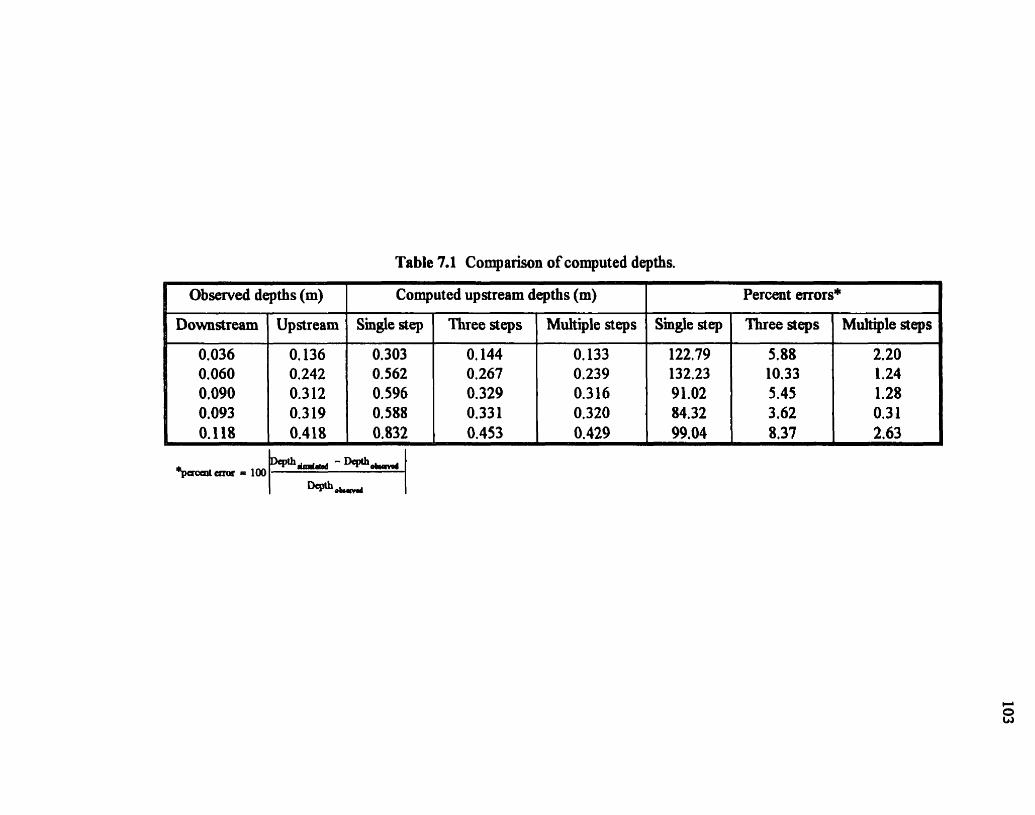
Table 7.1 Cornparison of computed depths.
1 Observed depths (m) 1 Computed upstream depths (m) I Percent mors*
Three steps Downstream
0.036 0.060 0.090 0.093 0.118
Upstream
O. 136 0.242 0.3 12 0.3 19 0.418
Muitiile steps
O. 133 0.239 0.3 16 0.320 0.429
Smgle step
0.303 O. 562 O. 596 O. 588 O. 832
Smgle step
122.79 132.23 91.02 84.32 99.04
Three steps
5.88 10.33 5.45 3.62 8.37
Multiple steps
2.20 1.24 1 .28 0.3 1 2.63

the fiction slope, both measured at the downsîream section 'Ihis implies that may be
long when the hydradic gradient is s u d , end may aIso be long when the downçtream
depth of water is large. This can be readily seai £iom Figures 7.2 and 7.3. The L for
different fiction dopes ranging from 0.00 1 to 1.00 have been plotted m Figures 7.2 and
7.3 for hypothetical downstream depths of w a t q yl, of 1 m, 3 m, 5 m, 10 m, and 20 m
for profiles simiiar to Ml and M2 water surfàce profiles in GVF, respective&. For a
particuiar depth of water, it can be seen from Figures 7.2 and 7.3 that the L- increases
with decreasing fiction dope. Also, for the same ection dope, the L,, is longer for a
higher depth of water at the downstream section. 1t cm also be seen fiom Figures 7.2 and
7.3 that, an L,, of not more than 16.66 km should be used m the computation of an M2
profile, d e n the fiction slope and depth of water at downstream section axe 0.00 1 and 20
m, respectiveiy. Such a long aiiowable reach length is not recommended m the n 4 c a l
.simulation of water surface profiles even for open ch81lfleIs. Lengths greater tha. 1600 m
(one mile) are seldom employed for even the moa gently dopmg and UIUform-section
rivers (Tavenq 1973). For neeper and less d o m rivers, reaches as shon as 400 m
(one quarter mile) or less are commody employed. The expressions for La, equations
[7.2] and L7.31, were derivecl on the premise that the cross-sectional variability between
the sections is negligile, m other words, the drain sections are d o m within the reach
considered. It would be rare to find a natural rock drain having d o m sections for more
than 1600 m. Therefore, for the numerical simulation of water surfàce profile through
rock drains, the numhmm allowable reach length should be determined by equation [7.2]
for draÏns having arbitrary sections, or by equation [7.3] for wide rectanguiar drains, when
Fr, is smaIL If the computed dowable reach length is more than 1600 m, m i,, =1600
m should be used m the computation.
When excessively long reach lengths have been surveyed m the field, it is common practice
to derive mterpolated synthetic crosîsections between the two m e y e d sections m order
to p e r d computation of the water surfiice profile. For the case of channels with prismatic

Rictiaa s l o p at chmtrem section
0.01 0.02 0.03 0.04 0.05 0.06 0.07 0.08 0.09 0.10
kiction s lope at dowtream section
Pkiction s lope at donastream section
Figure 7.2 La for wide rectanpuiar channeis, applicable to M2 profiles. (y1 is the depth of flow at downstream section )
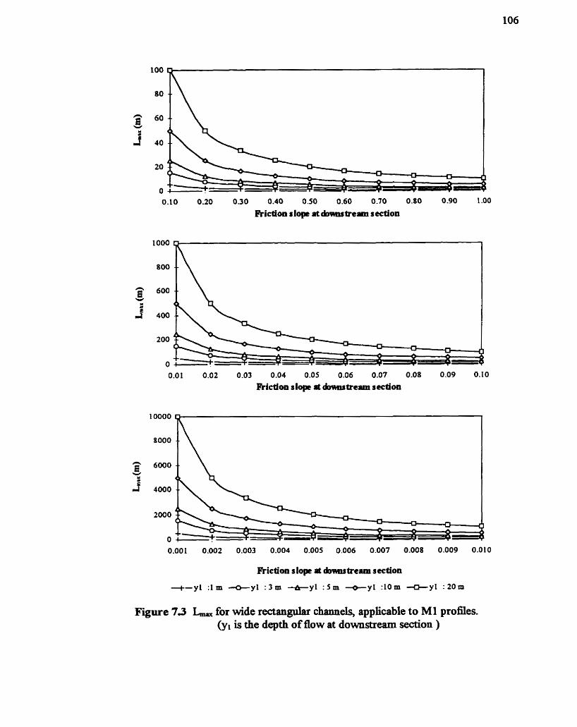
0.10 0.20 030 0.40 0.50 0.60 0.70 0.80 0.90 1.00
PLictIon slop at m t r e m n section
0.001 0.002 0.003 0.004 0.005 0.006 0.007 0.008 0.009 0.010
Pkictioa slop a chuStream section
+-y1 :l m -y1 : 3 m +y1 : 5 m '-=-y1 :IO m -y1 : 20m
Figure 7.3 L- for wide rectanpuiar chamels, applicable to Ml profiles. (y, is the depth of flow at downstream section )

cross-sections and d o m bed dope, the mterpolated mss-sections are exact. The
introduction of interpolated sections is also used for some non-prismatic natural charnels
when the van;;ib%ty between the cro~seztions is wahm certain limas. Where Stream
c r o ~ s x t i o n s are very hregular, mathematicaIiy mterpolated croçî-sections rarely reflect
actual conditions. The mor invohred is thexefore mdetemimte in this case. Ifsipnincant
Merences exkt between the observed and simulateci flow profiles, new cross-sections
may be surveyed at the points mdicated by the prehhary simulation. The entire profle
c m then be recomputed mcorporating the additional sections.
When the Bow regbne changes gradually fiom subaitical to d c a l , the magnitude of the
pore Froude number, k,,, gradua& mcreases and becomes unity at the critical depth.
Such a flow condition might prevail at the downstream exit &ce of rock drains. Under
such circumstances, when the magnitude of Fr, is Sgnincant, allowable reach length
should be computed by equation [7.2], depending on the profile type, and not by equation
17.31, wai for wide rectangular c h e l s . Theoretically, it is possile to model the water
surfàce profiles at or near the critical depth. Near the critical depth, an mcremental
mcrease in the vaiue of Fip win result m a corresponding decrease in I, At the criticai
depth becomes zero, as can be seen fiom equation 17.21. The physical interpretation
of L,- = O is that the curvature of flow profiles at the critical depth is large, so that a
dight movement m the hohn ta i direction will re& in a comespondingly large change m
depth of flow. Therefore, m order to similate the water surface pronle near the cntical
depth, the drain reach should be subdivided into a large number of very small sub-reaches.
7.3 Type II Uncertainty
Type II uncertahties, also termed "data uncertainties", are associated with uncertamties in
model parameters. Revious work by McBean and Perkins (1975 b) on open channel
flows with no porous media has shown that, ifproper care is taken with respect to cross-
section spacing, uncertainties arising fkom data description are considerably larger than

uncextainties mtroduced by numerical computations The mode1 developed m this study to
cnniilate water surfiice profile through rock drains is based on several parameters related to
the porous media. Uncertamty m assighg representative values to these parameters WU
have a significant effect m the sOmulated depth of flow. There are several procedures cited
and recommended m the literature for Type II uncertainty analyses. These procedures cm
be W e d mto two groups: fidi distniution anaiyses, and first and second moment
analyses Pettinger and Wilson, 1981). The fidl distnibution method be@s with a
complete specification of the probabüinic properties of d nondetembistic
mputdparameters of a system and attempts to s p e e completely the probability
distribution of the resuhs. The two most important fidl distnîution techniques are: (i) the
method of derived distn'butions and (ri) Monte Carlo s h h t i o n - The derived distnîutions
approach is an anaiytical method for deriving the probability distniution of a random
fùnction &en the distniutions of its independent variables (Benjamin and Corne& 1970).
The anaiysis becomes prohibitively complicated unless applied to simple systems with
relative@ Smple probabilistic properties. On the other han& the Monte Carlo method uses
a large number of replications of the system, with the parameters and mputs of each
&dation generated at random fiom thei. respective probability distniutions. The resuhs
of the simulations are compiled to fom estbates of the probability disÉniution of the
depth of flow. First and second moment methods assume that the fïra two moments
(mean and variance) are sufncient to characterize any random variable or function. First
and second moment methods usudy are applied m two diffèrent ways: perturbation andior
Taylor series expansion. In perturbation anaiyses the partiai differentiai equation
goveming any system is pemubed slightiy, yielding a new equation which govems the
random or fhictuating component of the system. First and second moment analyses based
on Taylor series expansions is the analyses of the mean and variance-covariance of a
random fùnction, based on its Grst and second-order Taylor series expansion. A schematic
of Type I I uncertahty analysk methodologies is shown m Figure 7.4.
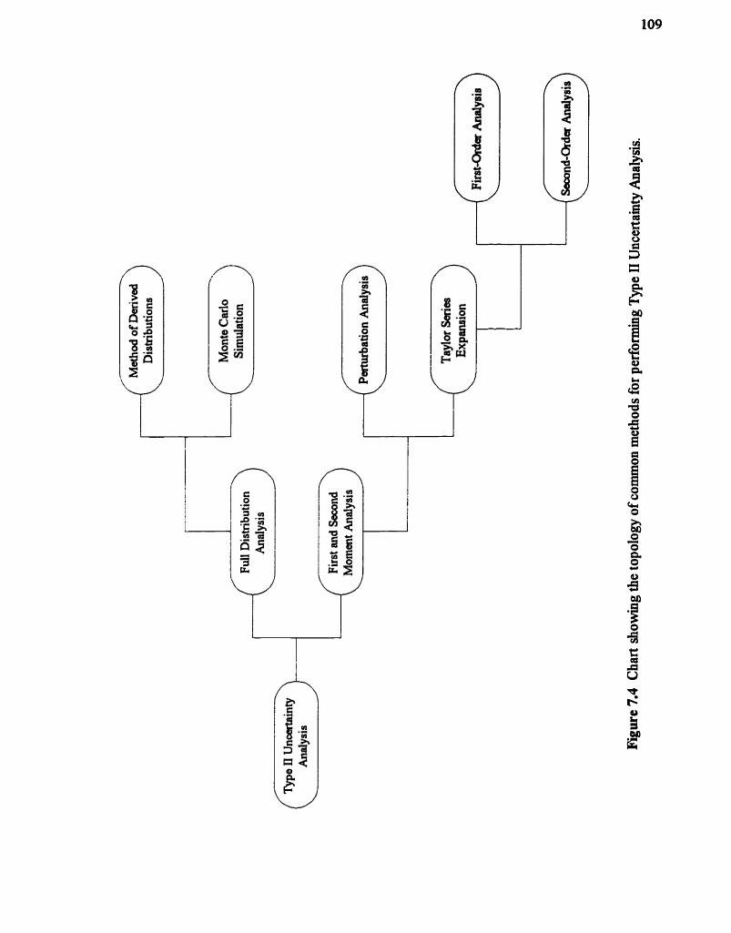

In this study the uncertainty m the sindatecl depth of fiow through rock drains associated
with uncertainty m model parameters was besiigated. The following section discusses
the components or the model parameters contn'buting to Type II uncertainties in computed
depths of flow and, then considers uncertainty analyses perfomed by (i) the fist and
second moment method based on Taylor series expansion and (ii) the fiill distri'bution
technique based on Monte Car10 simrulation. It is assumecl in an the analyses that the
model parameters are statisticdy mdependent.
7.3.1 Components contributing to uncertainty in computed depth
In order to identify the components contn'buting to uncertain9 in the computed depth of
flow, a rock drain of rectangular section may be considered. The average depth of water,
7, at any section of such a rock drain c m be deteRnmed by sohring either of the foflowing
two eqyations:
where: - B : average drain width, - Q : average discharge, - re : average shape coefficient, - W : average Wilkins' constant, - Kt : average value of Stephenson's fiction hctor, - 11 : average vahie of porosity, - d : average particle diameter, - 1 : average fiction dope.

Equstions 17-41 and [7.5] are based on the Wilkins and Stephenson equations, respectively.
Derivations of equations [7.4] and [7S] are provided at Appendix 6.
The mode1 developed m Section 4.2 solves equation [7.4] or [7.5] for the depth of water
at diBerent sections dong the rock drain. There are no explicit solutions to the above two
equations so an terative numerical scheme was employed to solve them When WiIkins'
equation is used it can be seen fiom equation [7.4] that the depth of flow at any section of
a rock drain is a function of seven independent variables, nameiy: drain width, discharge,
Wükms constant, shape coefficient, particle niameter, fkiction slope, and porosity.
Smnlarly, when the Stephenson e p t i o n is used it can be seen from eqyation 17.51 that the
depth of flow is a function of six mdependent variables: drain width, discharge, fiction
Bctor, particle diameter, fiction slope, and porosty. Uncertainty m estmoating these
mdependent variables will r e d m uncertainty in the sinnilated water surface profiles
through a rock drain.
7.3.2 Uncertainty analysis by the first and second moment methods
The assumptions underlying the first and second moment methods are that the important
information about the random variables (or fùnctions) of mterest can be summarized with
the mean representing the central or expected tendaicy of the variable (or fimction), and
the variance-covariance representhg the mount of variation around the mean (Dettinger
and W k n , 198 1). Unless the third moment (skewness) or higher moments of the variable
are relative@ large, they are generally of little interest. An example of a fimction fidfihg
this assumption is one which is normaüy distniuted. Such a function has zero skewness
and zero higher moments of odd order, and ail even-order moments cm be calculated fiom
the variance (Benjamin and Corne& 1970). Within the framework of the second moment
method it is not possible to test the assumption that the mean and variance-covariance fùlly
d e m i e the fundon. Thus, other methods, m partinilar full distriiution methods, should
be used to check whether the mean and variance-covariance d i c e .

As prwious.€y mentioned, the fnst and second moment rnethods can be applied by
perturbation and Taylor series expansion rnethods. Uncertahty analyses by the first and
second moment method based on Taylor series expansion can be grouped mto ikst and
second order anah,sis. First-order -sis CM be deiined as the &sis of the mean and
variancecovariance of a random fûnction based on its fkst order Taylor series expansion.
Second-order anaiysis refers to anaiysis of the mean based on a second-order Taylor series
expansion with the concurrent anasis of the variancecovariance restricted to use of the
fist order series expansion (Dettinger and Wüson, 1981). Denned in this way, the mean
derived fiom first and second order anaiyses may be different; the variancecovariance wiü
be the same.
In this study, the anabsis of uncertainty in smnilated depth of flow through rock drains by
nrst and second moment method was based on fkst-order Taylor series expansion.
7.3.3 First-order uncertainty analysis
Fist order uncertamty anaiyses, in general, can only be applied properly to nonlinear
systerns m which the coefficients of variation (CV's) are snall. These analyses are based
on the expected values of tnmcated Taylor &es expansions. If the tnincation error is to
be smaii, then the higher order terms m the expansion must be negiiglile. Either the higher
order derivatives or the higher order moments of the variables must, therefore, be srnaJi.
In Section 7.3.1, all the components contnbuting to uncertngity in the simiilated depth of
flow through rock drains were identified. Swen variables or model parameters were
identified which might cause error m simulated depths when Wilkins equation was used in
the model to compute the Ection dope. Siniilrirly, six variables or model parameters were
identified which might cause m o r m smnilated depths when the Stephenson equation is
used m the model to compute the fiction dope.

Let us denote the mcertainty m the smnrlated depth of flow contniuted by the j' variable,
Xj, of equation [7.4] or [7.5] by E,, . By applyjng first-order uncertaine -sis
- EX, -
where:
a, : standard devhtion of the j" variable, Xj.
When a i l the variables are statistically mdependent, the total uncertamty can be expressed
by the error propagation formula defhed m Section 2.5:
where:
% : standard deviation of the sinnrlated depth of flow,
N : number of mdependent variables contnîuting to uncertainty m simulated depth; N = 7 when the model uses W W s ' equation to compte fiction dope, and N = 6 when the model uses Stephenson's equation to compute fiction dope.
Thus, the uncertainty m the computed depth of flow CM be estimated by evaiuating the
magnitude of mdividual E ,, tenns and substituthg them mto equation [7.7] to obtain the
total uncertahty. Expressions for the terms, Le., the expressions for the contniiutions
of the Mirent mdependent variables to the unceriahty in Smulated depth of flow are
reported m Table 7.2. Derivation of ail the equations iisted in Table 7.2 are provided m
Appendix 6. Two sets of expressions for the E,, terms were derived, one set associated


wah the use of WïIbns' equation m the modei, and one set associated with the use of
Stephenson's equatioa
The total uncertahty m computed depth of flow, when Wilkins equation is used m the
model to calculate the fiction slope, cm be e v h t e d by substituthg equations [7.8] - [7.14] m equation [7.7]. Such substitution yields:
Similarty, the total uncertainty m computed depth of flow, when Stephenson equation is
used m the model to calculate the fiction slope, can be evahmted by substitutmg equations
[7.15] - 17.201 m equation 17.7. Such substitution yields:
it can be seen fiom equations [7.22] and [7.24] that the more haors that are added m
terms of uncertainty, the greater the total uncertamty m the computed depth. In this
study, the first-order uncertainty equations were deduced for a rectangular draE
geometry. When particular geometries that Wer significantly fkom the rectangular
geometry need to be mvestigated, they can be approximated by suitable geometric shapes
and a new set of eqytions showing the relationship between geometry and other
variables, and can be derived by smiilar procedure descrîbed m this study. M e r
introduction of these equations mto forms equivalent to equation [7.4] and [7.5], would

eaable an analyst to employ the gaieral first-order scheme in the same manner as outlined
hereia It must be ranembered that the anaSgs p d o d in this study assumed the
validicy of a onedirnensiod formulation for the flow normal to the flowthrough area. It
shodd also be remembered that the first-order unaxtahty an- perfomed m this shidy
did not consider any uncertainty m the starting depth of flow m the SSM numerical
scheme.
It is difiicuit to estimate the coefficient of variation of fiction slope. However, sensaMty
analyses showed that compared to the range of conmiody found coefficients of variation
for the discharge and other dependent variables, the enor m the fiction slope had a minor
effect on the results. Therefore, m the applications of the uncertainty equation to a field-
sale rock drain, the coefficient of variation of the fiction slope can be neglected. Under
these cirnimstances, whai the Wilkins equation is used m the model to calculate the
fiction dope, the total mcertainty eqyation becomes:
Simtlatly, when the variation m friction dope is neglected, and when the Stephenson
equation is used m the model to calculate the fiction slope, equation [7.24] becomes:
7.3.4 Sensitivity of uncertainty in computed depth to model parameters
The model parameterdcomponents contrîîuting to uncertainty m simulated depth of flow
through rock drains were identi£ied m Section 7.3.1. The equations descnbmg the
contniutions of these model parameters were derived m Section 7.3.3. B efore pedormhg
uncertainty analysis on eqerimentally-deteminecl -ter &ce profiles through the
model rock drain, it was of mterest to find out the relat-mive con~ntnbutions of the various
individual mcertainties to water SUTfàce profile variability. In ordder to achieve this, each
parameter was assigned m tum a CV of 0.10 while holding an others to th& respecthg
mean values, with CV = O. In this way, sinnùated profiles with f 1 standard deviation
bands were generated using equations 17.73 - [7.20]. Plots of these hypothaical smnilated
water surface profiles with phidminus one standard deviation bands are presented m
Figures 7.5 and 7.6. The water surfàce profile and the uncertahty bands were determined
for an arbitrary selected discharge of 2.44 U s through a model rock drain of dimensions of
the eqerimental drain m the TUNS hydraulics hboratory. The staning depth at the exit
face for the discharge of 2.44 Us was that obtained fiom the experiments perfonned on
the model rock drain. For the simulation of these water d c e profiles the mean vahies
of different model parameters (porosity, particle diameter, Wilkins' or Stephenson's
constant, and shape coefficient) mentioned m Chapter 5 were used. Figure 7.5 represents
the condition when the Wilkms equation was used by the model to compute fiction slope
and Figure 7.6 represents the condition d e n the Stephenson equation was used to
compute the fiction slope. It can be seen fiom Figure 7.5 and £iom equations 17.81 - [7.14] that porosity had the maximum band width as compared to the band widths of the
other model parameters. Evidently, when the numericd model used Wükms' equation as
the fiction slope eqyation and when the variabilities of all the model parameters were the
same, the contnoution of porogty to the uncertainty in simulated profiles was the greatest.
Simi?afly, it can be concluded from Figure 7.6 and equations [7.15] -17.201 that, when the
mode1 used the Stephenson equation as the headloss equation, the contributions of
porosity, discharge, and drain width were equal and made the largest c o n t n i o n to the
uncertainty in smmilated water mfàce profiles.
In order to extaid the clarincation of the relative contniution of various model parameters
to the mcertainty in computed depth, the deviations firom both the observed and mean
depths (computed using meadoptimal model parameters) as percentages of upper and


% al .ilh * ris I
Distance downstream (ni)
ünculainty due to pariidc dia - 225
0.0 0.3 0.6 0.9 1.2 1.5 1.8
Distance downstream (m)
Distance downstream (m) 0.0 0.3 0.6 h9 1.2 1.5 1.8
Distance downstream (m)
&ccrtainty duc toparosity
a0 0.3 0.6 0.9 1.2 1.5 1.8
Distance downstream (m)
Figure 7.6 Relative contribution of mode1 parameters having equal coefficient of variation to uncertamty m simulated profiles. Headloss computed by Stephenson's equation (dotted lines represent one standard deviation above and below the
CI,
siiulated profile). F e
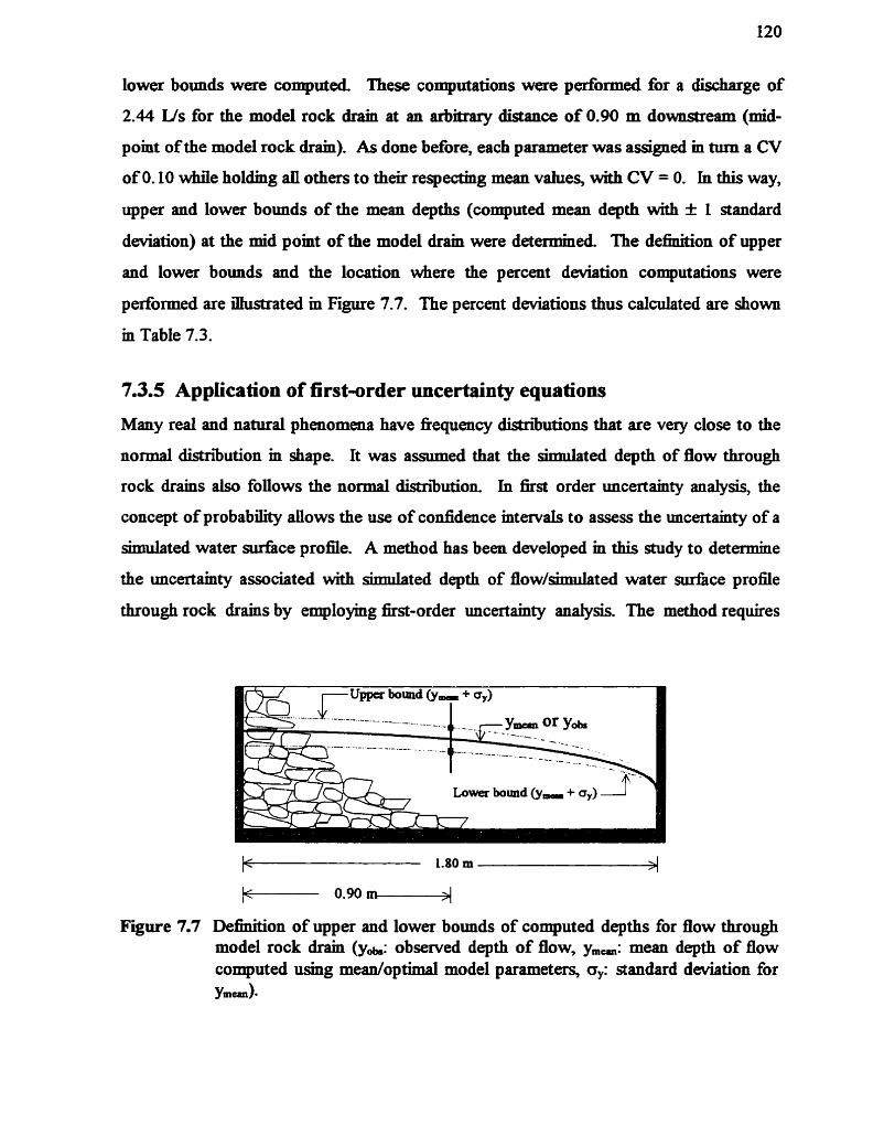
lower bounds were computed. 'Ihese computatiom were pdormed for a discharge of
2.44 Us for the model rock ârain at an arbitrary distance of 0.90 rn downstream (mid-
point of the model rock draiu). As done before, each parameter was assigned in tum a CV
of O. 10 while holding ail others to their respecting mean values, wiîh CV = O. In this way,
upper and lower bounds of the mean depths (computed mean depth with f 1 standard
deviation) at the mid point of the model drain were determined. The dennition of upper
and lower bomds and the location where the percent deviation computations were
perfiormed are ihstrated in Figure 7.7. The percent deviations thus calculated are shown
in Table 7.3.
7.3.5 Application of first-order uncertainty equations
Many real and natural phenomena have fkequency distniutions that are very close to the
normal distrr'bution m shape. It was assumed that the simulated depth of flow through
rock drains also follows the normal distniution. In ikst order uncertainty analysis, the
concept of probability ailows the use of confidence mtervals to assess the uncertainty of a
smnilated water surtiice profile. A method has been developed in this shidy to determine
the uncertainty associated with Smulated depth of fiow/smnilated water surfhce profile
through rock drains by employing first-order uncertainty analysis. The method requires
Figure 7.7 Definition of upper and lower bounds of computed depths for flow through model rock drain (yh: observed depth of flow, y,,: mean depth of flow computed using meadoptimal model parameters, a,: standard dwiation for Y~=J

- - - e C I e
2 = ! S " ' " m m m

the output fiom the numerical model developed in Section 4.2 together with the
application of the fins-order uncertainty equations, derived m Section 7.3.3. By
employing the proposed method, mstead of a unique upper and lower uacertainty bound
value, confidence mtervals were obtained. In this study, a standard deviation intend o f f
1 was use& which implies about 68.27% of the m a under the nodGaussian
dimiamion.
The uncertamty in the computed depth of flow through rock drains can be determineci
using the equations [7.25] or [7.26]. As previously stated, the data for a prototype rock
drain was not available during the course of this shidy. This prechded the use of the
methodologies developed in this shidy to genenite uncertainty bands for water surface
profiles through a field-scale rock drains. Howwer, an effort wes made to dwelop such
unceztahty bands for water surface profiles through mode1 rock drains, buih as a part of
this shidy.
It was felt that the porosity of the porous media of the model rock drain and the drain
width were measured accurateiy in this study (relative& speakmg) so that the coefficients
of variation of porosity, CV., and drain width, CV& were taken as zero. The variabüity of
Wilkins' constant was also taken zero m this study m order to make the scope of
computational work more manageable. When these assumptions are applied to equations
[7.25] and [7.26], the total uncertainfy equations for Smulated depth become:
Equations [7.27] md [7.28] represent the conditions when Wilkins' and Stephenson's
equations are used, respectively, to compute the fiiction dope. It shonld be remembered
that eqyations [7.27] and 17.281 are applicable on& to conditions similar to those of the

study performed herein, For a prototype rock drain the uncertainty in simulateci depth
should be deter-ed using equation [7.25] or [7.26].
Umig the equations 17.271 and [7.28], Snnilated water sudice profle f 1 standard
deviation bands for flows of 1.60 Us, 2.39 Us, and 3.75 Us passing through the model
rock drain were generated. Simiilations and subsequent analyses were based on the data
obtained fiom the laboratory eqeriments on the mode1 rock drain. In order to determine
the coefficient of variation of particle diameter of the porous media, CVd, the intermediate
axes of 100 randomiy selected rock particles were measured The value CVd thus
obtained based on 100 particle diiimeter was assumed to be representative of the entire
porous media. As previously mentioned discharge was measured by three methods: (1)
vohunetrically (2) by V-notch, and (3) by transducer. These discharge values were used
to compute the coefficient of variation of discharge, CVQ, for each nm. The coefficient of
variation of the shape coefficient, CV, . and coefficient of variation of Stephenson fiction
factor, CV&. were d e t d e d by calibrating the nu-cai modei. The coefficients of
variation of above mentioned four model parameters are reported in Table 7.4. The
associated uncertahty bands are presented m Figures 7.7 - 7.8, together with the
simulated and observed water d c e profiles. Figure 7.7 represents the condition when
Wilkins' equation was used in the model to compute the fiction dope, and Figure 7.8
represents the condition den Stephenson's equation was used to compute the fiction
dope. The bands *ch are shown by dotted lines in Figures 7.7 - 7.8 represent the
combined effect of d model parameters on uncertainty m simulated water surface profiles.
It can be expected that the simulated water surface profiles for the discharges of 1.60 Us,
2.39 Us, and 3.75 Us will lie withm these bands about 68.3% of the t h e . For non-Darcy
water surfice profiles through a field-scale rock drain, uncertainty analysis can be
performed ushg the procedure and equations developed in this study. It can be seen that
application of equation f7.251 or [7.26] requires the coefficients of variation of several
bput parameters, nameiy: discharge, drain width, shape coefficient, Wilkins' or
Stephenson's constant, particle diameter, and poro*. Uncertain9 about a @en
discharge value use& of &ch CVp is a measure, would depend on the ori@ of the flow,

Table 7.4 Computed~calibrated CV's of different model paramam used in generating
total uncertainty bands.
Wilkins
Parameters
Stephenson
Parax.net ers
ie. how t was obtained Ifit was obtained by a field measurement ushg dye mjection or a
current meter, the uncertainty would depend on the elements of the technique used.
Pelletier (1988) reviews the various components of uncertahty in flow data obtahed using
conventional hydrometry. If the discharge of mterest is based on a flood frequency
analysis of historical flows and has a r e m period attached to it, a confidence band for the
flood fiequency m e rnay be generated statistically and this would form the basis for CVP
of the flow of interest. The coefficient of variation of drain width can be deteniiined fiom
the flood plain geometry (by direct measurement). The coefficients of variation of shape
coefficient, Wilkins' or Stephenson's constants, particle diameter, and porogty can be
estimated kom the caliration of the model ushg the observed data relating to water
surface profiles through rock drains, if such data is available. A procedure for domg this
was descri'bed in Section 5.4.

Distance downstream (m)
Distance doenstream (m)
0.0 0.3 0.6 0.9 1.2 1.5 1.8
Distance downstream (m)
Figure 7.8 Plots of sinmlated wates surfkce profiles by the mode1 I 1 o band fiom fit- order uncertainty analysS. Head loss computed by Wilkins' equation (dotted Lines represent one standard deviation above and below the gmuLated profle).

0.0 03 0.6 0.9 1.2 15 1.8
Distance dowostream (m)
Distance downstrearn (m)
0.0 0.3 0.6 0.9 1.2 1.5 1.8
Distance downstream (m)
Figure 7.9 Plots of smiulated water surfece profles by the mode1 f 1 o band fiom fist- order uncatamty anaiysis. Head loss computed by Stephenson's equation (dotted iines represent one standard deviation above and below the sinnilated profile).

In cases where there is no data to p d the model to study the uncertainty, a mean vahie
of porogty of 0.40 c m be used m most anaiyses (since the range of porosity for the
porous media of most rock drains is 0.30 - 0.50) with a coefficient of variation of 0.20.
The value of R m equation [7.12] for most field-scale rock drains ranges nom 1.71 to
2.00, for porosities of 0.30 to 0.50. An average vahie of R = 1.83 cm be used for most
emor analyses, which corresponds to a porogty of 0.4 1. Coefficient of variation and mean
value of particle diameter can be estimated with a reasonable accuracy by visual mspection
of the rock drain. For other parameters (sbape coefficient and Wilkins' or Stephenson's
constant) mean values can be taken fiom the literature as their suggested values for rocks
and the coefficients of variation can be taken arbitrady as 0.20.
7.3.6 Uncertainty analysis by Monte Carlo simulation
The Monte Carlo method can be broadiy dehed as any technique for the solution of a
model ushg random numbers or pseudo-random numbers. Random numbers are
stochastic variables &ch are d o @ distniuted on the interval [O, 11 and show
stochastic mdependence. Pseudo-random numbers are generated by applying a
determniistic algebraic formula which resuhs m numbers that, for practical purposes, may
be considered to behave as random numbers, Le., to be unifody distriiuted and mu*
mdependent. This mdependence +lies that the "cycle tength" is sdkiently long. The
cycle length is the number of pseudo-random numbers that are generated before the same
sequence of numbers is obtained again. There are a number of algorithm available m the
literature for pseudo-random number generation. The advantage of pseudo-random
numbers over purely random numbers is that the computer cm generate pseudo-random
numbers ushg any of these algonthms, so that no storage of a large table or random
numbers is needed Smce a computer, being a deternenistic machine, c m only produce
pseudo-random numbers, the tenn 'ïmdom number" will refer to pseudo-random number
here now onwards.
The principal application area of the Monte Car10 method is distri'bution samphg, which
Mergenthaler (1961) calls model sampling. Distriution sampling has been m use in

mathematical statisiics for decades. The purpose is to k d the distri'bution, or some of the
parameters of the distribution, of a stochastic variable of interest. This stochastic variable,
cded the output variable, is a hown fûnction of one or more o h stochastic mput
variables which have known distriiuti~ns~ To esthnate the distriiution of the output
variable we draw a value for each of the input variables fi0111 their distniutions and
calculate the resutting vaiue of the output variable. Such sampiing is then repeated maw
times and this eventudy yields an estimate of the distniution. The method is readily
automated and can be applied to complicated distriiuted-paramete systems. A
disadvantage of Monte Carlo simulation is that the resuhs are never in a closed anaiytical
fonn that a derived distnbuton study strives for, and, the results are therefore not readily
tramdierable to a new situation. The numerous simulations required by Monte Carlo
techniques miplies a large computational burden. This computational effort will generaUy
place limitations (raised both by economics and expediency) on the accuracy with which
estimates of probabîiktic parameters can be obtaîned, Snce the accurscy of Monte Cario
techniques is an mcreahg fimction of the number of smnllstions c d e d out. Because of
these limitations on the use of Monte Carlo methods, kst order analyses of numerical
models are a naniral choice and can generaüy be made with an accuracy consdent with
the accuracy of the nunmical mode1 itseif
The mtent of this component of the shidy was to apply Monte Carlo simulation in
uncertainty analysis of the computed water surface profle, and compare the resuits with
those obtain fiom the FOUA m order to ver@ and evaluate the performance of the first-
order uncertainty analysis methodology. The generation of stochastic input variables,
simulation methods, and results of the simulations are outlined m the foilowhg sections.
A cornparison of resuhs obtained fiom fïrst-order uncertainty analysis and those obtained
fiom Monte Car10 ssmilation is provided m Section 7.3.7.

(i) n i e generatbn of siocha& input variables
Consider two stochastic variables XI and X2 which are assumeci to have independent
normal dïsûiiutions with mean and standard deviation ai for XI, and mean p2 and
standard deviation a2 for X2:
The central hnit theorem states that the sum of a large number of Bidependent stochastic
variables with the same distniution and a M e mean and standard deviation is
approximateiy normaüy distn'buted. Therefore, we might add tweive random numbers
assuming that twehe is high enough to yield an (approximately) nomu@ distri'buted
variable @&&en, 1974). The mean and variance of a random number r, as expressed by
equations [7.3 11 and 17-32], are 0.50 and 1/12 respectively. Hence, z defined m equation
[7.33] has mean O and variance 1, and Xthe central limit theorem holds, this z is normaiiy
distriiut ed.
Ifz has density N (O, l), then p + oz has den* N (p, 02). To generate Xi and X2 dehed
by equations [7.29] and [7.30] we may use:

In order to keep XI and XI mdependent, Mirent values of z needs to be used m equations
[7.34] and [7.35]. Each new mdependent vahie of z requires the generation of twelve new
random numbers ushg equation [7.33].
The procedure demibed above was employai m this shidy to generate the input variables
to the numerical model developed m Section 4.2. It is a weil-established â c t that if many
stochastic effects are simultaneoudy operathg on a system, the central liniit theorem
allows the collective effect to be represented as a Gaussian random variable. Like the
FOUA performed eariier, Monte Carlo Smulation assumes that the uncertainty m the input
variables of discharge, drain width, shape coefficient, particle diameter, porogty, fiction
dope, and Wkms' constant/Stephenson7s fiction factor contriiute collectively m the
uncertainty in the smnilated depth.
In thiç study uncertainty -ses by Monte Carlo simulation were performed for three
water surface profiles for the mode1 rock drain, designated as profiles 1, 2, and 3. Since
the performance of bot . Wilkins7 and Stephenson's equation m simuhihg water surface
profiles through the model rock drain was found to be almost the same, Monte Carlo
simulation was performed ushg oniy Wilkins' equation as the headloss equation. It was
anticipated that resuits obtained thus would be similar if Stephenson's equation were used
as the headloss equation. As stated prwiously for the model rock drain, when the Wilkins
equation is used as the headloss equation, the uncertainty m simulated depth of flow is
associated with three model parameters, name@ discharge, Q, particle diamder, d, and
shape coefficient, Te. The statistics which were used to generate these mput model
parameters are shown in Table 7.5. As previoudy mentioned, during the experiment on
model rock drain discharge was measured by three different methods. For each profile, the
mean vahie and standard deviation of discharge was computed fiom these three different
vahies of discharge.
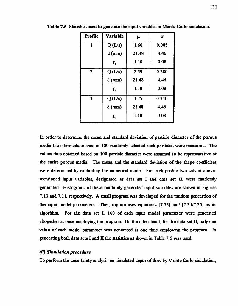
Table 7.5 Statistics used to generate the input variables in Monte Carlo smnlration.
Q (Vs) 1.60
d(mm) 21.48
Te 1.10
Q (Us) 2.39
d(mm) 21.48
Te 1.10
Q (Us) 3.75
d(mm) 21.48
Te 1.10
In order to determine the mean and standard deviation of particle diameter of the porous
media the intermediate axes of 100 randody selected rock particles were measured. The
vahies thus obtained based on 1 O0 particle Riameter were assumed to be representative of
the entire porous media. The mean and the standard deviation of the shape coefficient
were determined by c&irating the numerical model For each profle two sets of above-
mentioned mput variables, designated as data set 1 and data set II, were randomly
generated Histograms of these randomly generated mput variables are shown m Figures
7.10 and 7.1 1, respectively. A d program was developed for the random generation of
the input model parameters. The program uses equations [7.33] and [7.34/7.35] as its
algorithm. For the data set I, 100 of each mput model parameter were generated
altogether at once employing the program. On the other han4 for the data set II, only one
value of each model parameter was generated at one time employing the program In
generating both data sets 1 and II the statistics as shown in Table 7.5 was used.
(ii) Simulation procedure
To perform the uncertainty analysis on simuîated depth of fiow by Monte Carlo simulation,

For Profile 1
12 15 18 22 25 28 32
Clnss intend (mm)
For Profde 2
12 15 18 22 25 28 32
C l u s inttrvrrl (mm)
For Rofde 3
12 15 18 22 25 28 32 1.00 1-09 1.17 1.26
Clrss Interval (mm) C l u s inteml
Figure 7.10 Histograms of randomiy-generated mput mode1 parameters: data set 1.

For Profde 1
1.4 1.5 1 3 1.6 1.7 1.7 1.8
Clus intcrvril (Us) 12 15 18 21 24 27 3û 1.00 1.07 1-15 1-22
Clus Intcrvril (mm) aass intervrl
For Profde 2
Clus interval (Us) Class intcrval (mm)
For Profde 3
. .
3.0 3 3 3 3 3.8 4.0 4.3 4 3 13 16 19 21 24 27 30 0.99 1.08 1.16 1.25
C l u s intecwl (Us) Clus interval (mm) Clus interval
Figure 7.1 1 Histograms of randomly-gmerated mput mode1 parameters: data set IL

the model equations were SOM repeatedly. From these repeated model executions,
various statistics such as mean, standard deviationharhce of the icimiilated depths at
Merait locations dong the fiume were calculated. As previoudy stated, for the data set 1
each of the model parameters (Q, d, and Te) were generated 100 times at once (total 300).
Each model execution was performed combining randordy any three variables fiom these
generated 300 parameters. This procedure was foïlowed for the Monte Carlo simiilation
of each of the three profiles. For the data set II model equations were solved using
randomly generated Q, d, and T. one at a tirne. The simulation was terminated after 100
such model execution. This procedure was foilowed for the Monte Carlo simulation of
each of the three profles. Thus, for three profiles (see Table 7.5) with two sets of data
(data set 1 and II) a total number of 600 model executions were pedormed m this study.
(iii) Resrrlts of Monte Carfo simulations
A large data base of water surface profiles was obtahed ushg Monte Car10 simiilation.
For each profile (Table 7.5) the numerical model was executed 100 times using the data
set 1 and II. The headloss was calcuiated m the model ushg W i s ' equation. The
model which employs the numerical scheme similar to SSM for open channel flow was
used, and the arithmetic average of the upstream and downstream dopes was used to
calculate the representative fiction dope between pairs of sections. Like FOUA, the error
bands (mean water surfàce profile h m Monte Carlo simulation i 1 standard deviation
bands) were generated for each of the three profles. Plots of the error bands for profiles
1'2, and 3 are shown in Figures 7.12, 7.13, and 7.14, respectively.
7.3.7 Cornparison of analyses by the first-order and Monte Carlo simulation methods
Both Monte Carlo simulation and the first-order uncertainty anaiysis methods have been
used extensive@ for estimahg Type II errors in aIl areas of civil engineering. For
example, Burges (1979) and McBean et ai. (1984) used the first-order uocertainty an*&
methodology in quantifLing the magnitude m uncertainty in flood plain delineation.

Gardner et al (1980), O'Neil et al. (1980), 07Neil and Gardner (1979), and Tiwari and
Hobbie (1976), used Monte Carlo anaIpes for estimahg errors m complex food-web
models in water quaüty modeiing. Occasionaily both methods have been used m the same
study (Burges and Lettenmaier, 1975; Montgomery et al., 1980, Scavia et al., 1981 etc.).
Assumed impiicitiy in the latter studies, and suggesîed explicitly elsewhere (Gelb, 1974) is
that Monte Carlo represents "ûuth'' and that it cm be used to check the accuracy of
approximations made in first-order mcertahty analyses. The intent here is to check
whether the fkst-order analysis and Monte Carlo simulation methods q u a n e the same
type of variabiiity m simulated water surface profiles. R e d s obtahed fiom such
cornparison would be used in suggesting the conditions for which each method should be
used and when they should be expected to agree.
The kst-order uncertamty analysis (FOUA) equation generated variab- in the model
output. In the FOU4 model output is referred to as the determsllstic solution for the
water çurface profle and can be generated independen@. Monte Carlo simulation
generated variabilily about a mean water sudiace profile fiom LOO model sbdations.
Observed water swfàce profiles, water surfàce profiles fiom the deterministic solution of
the model, and mean (Monte Carlo) water surface profiles are ilhistrated in Figures 7.12 to
7.14 for pronles 1 to 3, respectively. For each profle the left and middle graphs represent
uncertahty analyses by Monte Carlo sindation and the right graph represent output by the
first-order analysis. In order to compare the results of the error analyses, the SSE7s and
the error-bound areas (&) associatecl with the first-order analysis and Monte Carlo
simulation were computed The values of & and SSE are reported m Table 7.6. The
definition sketch for & is shown m Figure 7.15. From figures 7.12 - 7.14 it c m be seen
that mean water -ce profiles fiom Monte Carlo simillation and water surface profiles
f?om the deterrninistic soiution of the mode1 both track the observed water surfàce profles

Monte Carlo simulation Data Set - 1
r- Mean WSP from
0.0 0.3 0.6 0,9 1.2 1 1.8
Distance downstream (m)
Monte Carlo Simulation Data Set - II
Floor of flume
1.8
0.0 0.3 0.6 0.9 1.2 1.5 1.8
Distance downstream (m) 0.0 0.3 0.6 0.9 1.2 1 1.8
Distance downstream (m)
*sec Table 7.5
Figure 7.12 Uncertamty bands for profiie 1 generated fiom the Monte Carlo simiilation and the kst-order uncertamty anatysis. For the Monte Carlo simulation dotted Lmes represent f standard deviation about the mean of 100 simulated water surfece profiles. For the hst-order uncertainty analysis the dotted h e s represent f standard deviation about the water d a c e profiie found fkom the deterministic solution of the mode1 (MCS: Monte Carlo simulation, WSP: water surface profile).

Monte Carlo simulation Data Set - 1
- Floor of flume
1.8 .i , , ,
Monte Carlo Simulation Data Set - II
-FIOO~ of flume 1.8 1 r 1 1 1
2.3 3 solution of the modal
0.0 0.3 0.6 0.9 1.2 5 1.8 0.0 0.3 0.6 0.9 1.2 1 1.8 0.0 0.3 0.6 0.9 1.2 1.5 1.8
Distance downstream (m) Distance downstream (m) Distance downstream (m)
*sa Table 7.5
Figure 7.13 Uncertamty bands for profile 2 generated fiom the Monte Carlo simulation and the fkst-order uncertamty anaiysis. For the Monte Carlo simulation dotted h e s represent I standard deviation about the mean of 100 simuiated water surface profiles. For the kt-order uncertainty analysis the dotted h e s represent f standard deviation about the water surface profile found fiom the deterministic solution of the mode1 (MCS: Monte Carlo simulation, WSP: water surface profile).


satkfàctorily and similarly (see also Table 7.6). The SSE's for each of the three profiles
wmputed for Monte Carlo sbmhtion and the kst-order uncertainty @sis are s m d and
they do not Vary Sgnificady fiom each other. From the resuhs obtsined fiom this study it
is very difEcuh to reach a conclusion regarding which water surfrice profiles (fiom the
Monte Carlo nmiilatiodfiom the deterministic solution of the model) are better estimates
of the observed water surfàce profiles Snce observed water surfiice profles are also
subject to mors. The causes of these errors in observed water surnice profiles were
explained m Section 5.6. However, it can be conchxded that both Monte Carlo mean and
the determiaistic solution of the model represent the observed water su&ce profiles
satidàctorily.
v
Longitudinal Distance (m)
Figure 7.15 Definition sketch of error-bound area, &. FP is the mean water surfàce profde fiom Monte Cario grrmlation or the water surfàce profile fiom the determmistic model solution. 4 represents the standard daiation of depth fiom Monte Carlo simiilation or the first-order uncertahty anaiysis
Variancelsiandard deviation esthates of the depth of flow at Mirent locations of the
model rock drain fiom the two approaches are similar. It can be seen nom Figures 7.12 - 7.14 that a similar spread about the mean water surfàce profile is represented, wiiether

fkom Monte Carlo simulation or nom the ht-order analysis. There are, howwer, some
differences between the two estimates. The error-bound area, Ao, is an estimate of the
variance. The definition of the error-bound ana is different for the two approaches. For
the Monte Carlo simulation, & represents the error-bound area m u n d the mean water
h c e profile. For the first-order adysis it represents the area around the mean water
surface profile generated fiom the det erministic sohrtion. Dehed m this way (ahhough
they represent two Mirent areas) they both represent the variab- in the simulated
mean water surface profle. The vaiues of & for all the three profiles are listed in Table
7.6. In this conte* average daiiations fiom the observed depths and the deternmiistic
solution of the model for the upper and lower bounds were also computed These are
shown m Tables 7.7 and 7.8, respective@. D e w o n of the upper and lower bomds is
provided m Figure 7.7. It can be seen fiom Tables 7.7 and 7.8 that the deviations
açsociated with kst-order uncertahty analysis were ahvays foimd to be greater than those
associated with Monte Carlo simiilation. The Werences are not very si@cant,
however. The differences between the variance estimates and deviations for Monte Carlo
simulation compared to first-order anaiysis cm be attriiuted to the following causes:
1. the deteimmwc and stochastic mean trajectories were somewhat different,
2. the kt-order analysis employed a first-order hearization of the model, whereas the
Monte Carlo anaiysis used the fiiny non-hear model,
Table 7.6 Cornparison of error bound areas and SSE's by kst-order uncertainty anaiysis and Monte Carlo simulation methods.
Error bound area, & SSE
(X 104 m2) (X 10-~ m2)
MCS* FOUA** MCS FOUA
Profile Data set 1 Data set II Data set I Data set II
1 568.49 579.37 787.15 6.78 4.59 9.80***
2 1074.49 774.77 1369.17 21.35 15.65 16.22
3 1064.28 1102.95 1622.22 8.5 1 18.00 8.24

3. there is a bAamental difference in the mterpretation of variances m the two
approaches.
Table 7.7 Average dewiations fcom the observed depth of upper and lower bounds of Morne Carlo simulation and îïrst-order uncertainty analysis.
Table 7.8 Average deviations nom the model solution of upper and low Monte Carlo simulation and nrst-order uncertainty ana&&.
MCS 1 FOUA
Profile Upper Lower Upper Lower
bound bound bound bound
1 10.86 7.33 12.25 12.25
2 8.23 10.46 16.11 16.11
3 10.7 1 5.56 14.28 14.28
r bounds of
Variance/standard deviation estimates are biased by the mean vaiue because variance is a
dimensional quantity. To reduce the effect of Wering mean trajectones, the coefficients
of variation which represents percent deviation (100o/p) fiom the mean were computed
for Smulated depths of flow through the model rock drain for ail of the three profiles, for
both Monte Carlo and the first-order analysis. Rearranging equation [7.27] yields:

For a particutar profile d the temis m the right hand Sde of equation [7.36] are constant.
This fkt wiil r e d t m a straight line plot pardel to the horimntal axis if a graph of CV's
(of depth of flow) versus 1ongaUdina.l distance is drawn for the first-order analysis. Plots
of the same variation for the Monte Carlo method, however, d r e d in curvilinear hes.
Plots of the variation m the CV's of depth of flow dong bed of the model rock drain for
both Monte Carlo and the first-order analyses are shown m Figure 7.16. This figure
shows the non-linear Monte Car10 and the Lmear nature of the fkst-order anaiyses. Figure
7.16 also fistrates that these estimates of variance, wen when scaled by the me- can
m e r considerably. It can therefore be conchided that diEering mean trajectories alone
was most likely not a major effect here.
As mentioned previously, Monte Carlo nnalysis invoives repeated solution of the non-
linear modeL On the other han& derivation of the first-order uncertahty equations
involves replacing the non-linear model (eqn. 2.26) by its Taylor series approximation (eqn
2.27). The discrepancies between the two estimates could be caused by the madequacy of
the hear approximation. The best way to examine this is to make cornparisons among the
variance estimates by Monte Carlo, fisi-order, and second-ordex uncertahty anaiyses.
Since the second-order propagation equation invohes second order partial derivatives
matrices which are cumbersome to handle, uncertahty an@& by the second-order
method was not perfonned in this study. In general it can be anticipated that the second-
order uncertaiuty analysis estimates would be closer to Monte Carlo esthates than the
first-order estimates However, inchidmg one higher-order t m m the În.6nite Taylor
series expansion does not guarantee a more accurate approximation. In a similar study
Scavia et al. (198 1 ) found that the differences m Monte Cario and the first-order variance

.--.-O W e : l (FOUA)
0.0 0.3 0.6 0.9 1.2 1.5 1.8
Distance downstream (m)
8 - - 0 M c : 2 (FOUA)
- O Rdile;l (FOUA)
- . 0 MC:^ (FOUA)
- A M e : 3 (FOUA) 3 - -
O
I -al (MCS)
-c:2 (MCS)
- A R d i l ~ 3 (FOUA)
-e:l (MCS) ('CS)
e c : 3 (MCS) -- I I r l
-c:3 (MCS) O 1 1 1 1
0.0 0.3 0.6 0.9 1.2 1.5 1.8
Distrince downstream (m)
figure 7.16 Plots of coefficient of variation of depth of flow along the bed of the mode1 rock drain fiom the first-order uocertainty analysis and Monte Carlo simulation. The left graph represents the anaîysis associeted with data set 1 and the right grapb represent s the analysis associated with data set Ii.

esthates m a lake eutrophication model may not have beei due to the hdeqyacy of the
iïrst-order linesrization.
The third explanation for the differences in variance estimates is related to the f imhenta l
diffaence m the two approaches. In deriving the first-order uncertain@ equation, the
mean squared deviation nom the true vahie of the depth of flow was examiaed In this
case the true vahie was the detenmnistic model soMon. The detemihktic model
represents the total system as long as its components have representative vahies. Thus,
the variance estimates 6rom the kst-order andysis represent variabiliiy around a typical
water surhce profile. Variance estimates fiom the Monte Carlo analyses m general,
masures the spread of the total population about the mean trajectory. Thus, the Monte
Carlo variance estimates represent the variability or spread of depth of flow around the
mean water suraice profile, rather than around a typical water surface profile, as m the
first-order case. Thus, the variances as cdcdated by the two techniques are not
necessady the same estimators. They estimate the same property only &en the
deterministic solution is representative of the total population or, in this case, when it
closely resembles the Monte Carlo mean trajectory.
Cornparison of the r e d s of the analyses reveals that variance estimates f?om Monte
Carlo and the iïrst-order analyses are generaüy simiiar, but have some Merences. The
investigations camied out m this study suggest that the Merences may be mainly due to a
combined effect of (1) dinêrences in estimates of depth of fIow (2) mors m the first-order
approximations (3) the fùndamental difference m the interpretation of the first-order and
Monte Carlo variances. The accuracy of Monte Carlo simulation is an increashg fimction
of the number of simulations carried out. The number of simiilations performed in this
study was 100. This number might not be adequate for an accwate estimation of the
variance of depth of fiow. This might be also a cause of the differing variance estimates
between the two approaches
When a numerical model is used to simulate the water surface profles through field-scale
rock drains the mors associated with those Snnilated water suinice profiles should be

estimatecl as weL These estmistes of mors affect the management decisions which
directiy or mdirectly influence various plaMing and design aspects of mines. In this study
two methods for error estimation for sinnilated water Surface profiles through rock drams
nameiy, Monte Carlo simiilation method and the &-order uncertamty anaiysis
methodology were presented m d e t d The Monte Carlo sirdation is a fidiy stochastic
approach of error anafysis. However, Monte Carlo simulation ofien ioiposes a high
computational burdm to the anest which is not feasble for practical application and
hence, avoided in most cases. On the other han& the fht-order uncertainty anaiysis
(FOUA) is an appropriate technique for most error analyses. When the input model
parameters of the numerical model are good representatives of the actual vaiues, water
surfàce profiies Smulated ushg those mput mode1 parameters would provide good resuhs
and the variance estimates by FOUA under such conditions represent variabilities aromd
those representative water surfàce profiles, and thus can be used to assign confidence
Limits. Although these estimates of variance may mer fiom those of Monte CarIo
sbmdation (for reasons discussed earlier), the ciifferences cm be anticipated to be not
great, and the estimates will provide general guides as to prediction confidence. To
explore the relative impacts of mors m various model mput parameters on model output
(water surface profiles in this case) variance, one ofien repeats the error analysk imder
difZering mput error scenarios. This procedure amplifies the required number of Monte
Carlo simulations, which resuits m excesive computer nm time. For this type of ' M a t -
if" analys& the £irst-order uncertainty equation has o* to be sohed once for each
scenario. It provides direct estimates of the sensitMty of model output variance to a
particutar set of uncertain mputs.

Chapter 8
SUMMARY, CONCLUSIONS, AND RECOMMENDATIONS
8.1 Summary and Conclusions
The principal objectives of this study, as outlined in Section 1.2, wae to: (a) develop a
numerical model for the gmulation of wata mf&ce profile through buried streams under
steady flow conditions, (b) identify the probable sources of mors associated with water
surfàce profile computation by this model, and (c) develop methods to quane some of
these errors. Ushg the models developed, the behavior of gradually-varied non-Darcy
flow through buried streams was studied and the applicability of the Manning equation to
water surface profile simulation through buried streams was mvestigated.
A detaiied statement of the origin of the one-dimensional dynamic equation for verticaUy
unconfined fîow through buried streams under steady state conditions was presented
(Appendix 2). The procedure foiiowed in deriving this eqyation for flow through burîed
streams or rock drains was smiilar to that generaily followed for GVF in open channek
The fom of the dynamic equation for flow m buried streams was show to be simüar to
that of the dynarnic equation applicable to open channels.
The numerical model presented herein is capable of simuiating non-Darcy water surfàce
profiles through buried streams. The performance of the model in simulating water
surfàce profiles under laboratory conditions was found to be satisfactory. The mode1
presented used Wilkins' or Stephenson's equation as the headloss eqyation. It was foimd
that the Wükms and Stephenson equations perfiormed eq- weii m simulatmg the
eqerimental water surface profiles through the model rock drain. It was observed that

when the vahie of Re was Iow, the pedormance of the WiIkins equation was better than
that of the Stephawn equation. For higher Re values the performance of the Stephenson
eqpation was foimd to be better than that of the Wilkms eqyation Ahhough the shortage
of field data prechided reachmg dennitive conclusions regarding the comparative
pdormance of the WiEns and Stephenson equations m predictmg water surfàce profiles,
5 is expected that the Stephenson equation would perform better under fù&-dweloped
turbulent flow conditions, Le., for non-Darcy flow through field-scale rock drains.
The performance of the numerical model was also evahiated under different fiction slope
averaging methods, namely the arithmetic average, geometric average, and harmonic
average. It was found that the performance of these fiction slope averaging techniques
was almost the same- At this stage it is difFicuEt to recommend a specific averaging
technique for a specinc type of flow profile for field-scale rock drains because there is a
severe shortage of data on which to base such conchi90ns. Based on the results obtained
in this study, it can be suggested that any of the above-mentioned fiction slope averaging
techniques would produce satisfictory estimates of flow through rock drains, provided
reach lengths are not excessive.
Stephenson (1979) suggested that for a fdy-dweloped turbulent flow through r o c m the
exit depth could be assumed to be equal to the d c a l depth (the depth at which the
specific energy is minimum). If this suggestion is followed for rectangular geometries, the
exit depth can be direct& computed by the critical depth formula applicable to non-Darcy
flow. Although completeiy fùlly-developed turbulent flow was not achieved through the
model rock drain, a cornparison was made between the observed exit depths and the exit
depths computed by this cntical depth formiila. It was found that observed exit depths for
various discharges and the correspondmg theoreticai exit depths found fiom the critical
depth fonda were not the same. It was also fomd that the magnitude of the difference
showed a weak kear trend, mcreasing with bcreasing discharge. For the non-Darcy flow
through the model rock drain the sireamlines were fair& steep near the exit (andogous to

being near the brink m open chmue1 flow). This violated the assumption of horizontal
flow m GVF. This breakdown of a key assumption of GVF was thought to be the main
reason for the Merence in exit depths.
The behavior of non-Darcy flow profiles through channels with varying cross-sectional
geometry was hvestigated both experimentaJly and computationdiy. A model rock drain
was bu& m a glass-wded fhme m the hydraulics laboratory of TUNS for conducthg the
expimentai investigations. To Srnulate to some degree the nanual conditions of a
prototype rock drain, the width of the model rock drain was varied m the fhime. It was
f o n d fiom the eqeriments that the response of non-Darcy flow pronles to changes m
crosîsections was not Smpiy malogous to that of open channel flow profiles under
s8nüar conditions. The di ' i f y m behavior of non-Darcy flow profiles to ordinary
GVF profles m open channels was explained with the aid of the energy equation. 1 was
fomd that the head loss withm a @en reach of the model rock drain was much larger than
that of an open channeL On the other hand, the velocity of flow through the porous media
was found to be very small compared to that of open channel flow, so that the velocity
head is generally negiigi'ble. Therefore, for the model rock drain the head l o s due to
fiction was always larger than the change m head due to the change m bed elevation.
Because of the large loss of head due to fiction, rises in depth of flow were not obsemed
for non-Darcy flow through the model rock drain d e n the £iow experienced an
expansion.
An effort was made m this study to investigate whether an existjng open channel software
package couid be adapted to water surface pronle simulation for buried streams. The
main cWk&y m applyhg such a package was identüied as the unavailabüity of a non-
Darcy fiction dope option. An mvestigation was therefore carried out to see whether a
uniform flow equation açsociated with ordmary (no porous media) open channels could be
adapted to non-Darcy flow profile simulation. Specifically, an attempt was made to
hvestigate the possbility of ushg the well-known Manning equation in non-Darcy water

surface profile computations. It was 8iitialS, sumked that a constant and relative@ hi&
value of Manning's would take into account an the porous media characteristics and
thereby permit such Smulations. Subsequentlyy the custom numerical model developed
earlier m this shidy was modified m order to allow t to compute the headloss using the
Manning equation. An optimum vaiue of = 1.75 was determined for the porous media
used m this study, based on data obtained fiom the eqeriments performed on the model
rock drain. It was observed that the approach of using Manning's equation with a fixed
n~ was not as accurate as the original model specificdly developed for use with a non-
Darcy fiow equation as the head loss eqyation. It is surmised that this is m . due in
general to the nict that the roughness characteristics associated with non-Darcy flow
profles differ si@cantly fiom that of open channel flow. In order to represent these
roughness characteristics, a depth-dependent Mamiing's n ~ , rather than a depth-invariant
n ~ , is necessary. Since al1 open channel software packages use stage-independent n ~ , the
application of such packages to simulahg non-Darcy flow profiles would result m a
certain amount of error. The amount of emor for a field-sale rock drain cotdd not be
quantifïed withm the fiamework of this study due to the shortage of data. It was found
that mstead of ushg constant (depth-mvariant) n ~ , a depth-dependent n~ Sgnificdy
improved the accuracy of the modified numerical modeL Since the option of d e p h
dependent n~ is not available m most ( h o t all) existing open channel software packages7
nich packages cannot generaUy be used dire* to simulate flow profiles through field-
scale rock drains.
An effort was made in this shidy to identifL the probable sources of uncertainty associated
with water surface profile simulation through rock drains. Ody Type 1 and Type II
uncertainty were considered m this work Type 1 uncertainties associated with the
simulation of water surface profiles through rock drains m general may arise nom:
formulation mors, numerical mors, and mors r e d g from the spacing and alignment
of cross sections. Uncertainty m simulated non-Darcy profiles associated with cross-

section spacing was mvestigated m this study. An equation for maimmun dowable
diSIance to be used m the numerical model between any pair of sections was derived. The
performance of this equation was eXammed and show to be usefiil in mhhkhg error m
shdating non-Darcy water SUTfàce profles through rock drains
Type II uncertainties, also temed ''data uncertainties", are associated with uncertainties m
model parameters, and were also mvestigated A comprehenshe list of techniques
available for Type II uncertainty anaiyses were presaited herein, When Wilkins' equation
is used, the depth of flow at any section of a rock drain is a fimction of seven independent
variables, narnely: drain width, discharge, WiIkins' constant, shape coefficient, particle
diameter, fiction slope, and porosity. Similarly, when the Stephenson equation is used,
the depth of flow is a fùnction of six independent variables: drain width, discharge, fiction
fiidor, particle diameter, fiction slope, and porosity. Uncertainty m estimahg these
independent variables resuhs m uncertainty m the simuIated water surfhce profiles through
a rock drain.
In order to quantify the probable mor m the computed depth of flow through rock drains,
total uncertainty equations were derived ernploying the fkst-order uncertahty anaiysis
(FOUA) methodology. The FOUA equations presented were deduced for a rectangular
drain geometry. When pdpamcular geometries that m e r significantly fiom the rectangular
geometry are to be mvestigated, they can be a p p r o h t e d by suitable geomenic shapes
and a new set of equations showing the relations@ between the geometry and the other
variables. These relationdqs can be derived ushg a procedure similar to the one
d e s d e d herein. This would enable an analyst to employ the FOUA m the same manner
as outlined in this study. It must be remembered that the an@& performed m this study
assumed the validity of a one-dimensional formulation for the flow normal to the
flowthrough area. It should also be remembered that the FOUA performed m this study
did not consider any uncertainty m the starting depth of flow in the numerical scheme used
to generate water sd3ce profiles.

A simplüied fonn of the total uncertainty equation was applied to qpantify the uncertainty
associated with the water stufàce profles Smulated for the model rock drain. Uncertainty
analysis for the model rock drain was also pedormed by Monte Car10 shmhtion (MCS).
A comparative study was performed between the r e d s obtained fiom FOUA and those
obtahed fiom MCS. It was found that the variance estimates nom the two approach
differed somewhat f?om each other. The different variance estimates fiom the two
approaches were a t t n i e d to the following causes:
1. deterministic and stochastic mean trajectories differed somewhat,
2. the first-order nnalysis employed a frst-order hearization of the model, whereas the
Monte Car10 anaiysis used the fu4r non-linear model,
3. there was a fundamentai difference in the mterpretation of variances m the two
approaches.
In general, Monte Carlo simulation is a fiilh/ stochastic approach for error analysis which
oftm imposes a hi& computationd burden on the analyst which is not feaslle m some
practical applications, and hence avoided for in some cases. Fist-order uncertamty
analysk is an aiternate technique for error anaiysis suitable for cases wherein the model
parameters are representative of the actual values. In such cases, water surface profiles
Smulated ushg these input model parameters would provide good resuhs and the variance
estimates by FOUA under such conditions would represent variabilities aromd those
representative water surface profiles, and thus can be used to assign confidence limits.
Although these estimates of variance might differ fiom those of Monte Carlo simulation,
the Merences d not be great, and wiil provide a guide as to prediction confidence.
8.2 Recommendations
The following aspects are recommended for friture study

(1) Unsteady £iow through rock drains
The study reported herein was eqerHnentally and computationally resbricted to cases of
steady flow. It would be desirable to investigate unsteady flood waves through rock
drains, experimentally as weil as numerical@ It is expected that such unsteady waves will
be damped out quickly by the extreme roughness of the coarse rock makmg up the drain.
(2) Failure of rock drains
The height of rock drains fomed due to continuous mining operation exceeds 50 m in
most cases. These rock drains are sometimes associated with large-sale *es which
can cause death(s) of minhg pers01meL In some cases the cause of such aiihires is pure&
"geotechnical" m nature. However, fàihues are also associated wah elevated water depths
through the drains, especialy at the downstrearn toe. It is therefore desirable to
mvestigate the stabiiity of rock drains fiom a geotechnical pomt of view, havhg
knowledge of the position of the mtemal water levels. Considerable guidance can be
found herein regardmg the position of these water levels.
(3) Transport of fie particles through rock drains
The velocity of flow through rock drains is low compared to that of true open channe1s. It
is therefore desirable to mvestigate whether such sxnall velocities are able to create enough
turbulence to dislodge fine particles fiom the void spaces in coarse porous media. The
small velocity of flow might cause gradua1 deposition of fine particles in the bed of the
drah, causing blockage of the flowthrough ara, especially if supplied fkom the upper
elevations of the rock drain.

REFERENCES
Arcement G.J. and Schneider V.R 1989. Guide for selectmg Manning's roughness
coeficient for naturai channeis with flood plains. USGS Water Suppiy Paper no. 2339,
USGS, Denver, Colorado, p. 38.
Barnes HH 1967. Roughness characteristics of natural channels. USGS Water Supply
Paper no. 1849, US Govt. printing office, Washington DC, p. 2 13.
Benjamin J. R and CorneIl C. A 1970. Robab-. Statistics and DeciSon for C W
Emgineers. McGraw-Hill Book Co., New York
Bnmner G.W. 1995. HEC-RAS River An- System, User's M a n d Water
Resources Consuhg Senices, Vacade' California, p. 1(1) - 8(20).
Burges S.J. 1979. An*& of uncertainty m flood plah mappmg. Water Resources
Butletin, VOL 15, no. 1, p. 227 - 243.
Burges S.J. and Lettenmaier D. P. 1975. Robabilistic methods m Stream quaiity
management. Water Resources Bulletin, VOL 1 1, p. 1 15 - 130.
Campbeil D.B. 1989. Some observations relevant to the performance of flowthrough
rock drains. 13" annual B.C. Mine RecIamation Symposium, 7 - 9 June, BiTech,
Vancouver, B.C., p. 119-128.
Chapra S.C., and C a d e R P. 1988. Numerical Methods for Enaeers . McGraw-Hü1,
New York.
Chow V.T. 1959. ûpen Channel Hvdraulics. McGraw-Hü1 Book Co., New York, p. 2 17
- 296.

Comeil C. k 1972. First-order an@& of mode1 and parameter uncertainty.
International Symposium on Uncertainties m Hydrologie and Water Resource Systems, p.
1245 - 1275.
D h g e r M. D and Wilson J. L. 1981. First orda a d y s i s of uncertahty m numerical
models of groimdwater flow, Part 1: mathematical development. Water Resources
Research, VOL 17, no. 1, p. 149 - 161.
Ergun S. 1952. Fiuid flow through packed cohmms. Chernical Engineering Rogress, VOL
48, no. 2, p. 89.
Fand R M. and Thmakaran R 1990. The Ïnfiuence of the w d on flow through pipes
packed with spheres. ASME Journal of Ruid Engineering, VOL 112, p. 84 - 88.
Feldman A. D. 1981. HEC Models for Water Resources Simulation: Theory and
Eqerience, Advances m Hydroscience, VOL 12, p. 297 - 423.
French R H. 1994. &en Channel Hvdraulics. Mcûraw-HiIl Book Co., New York, p.
195 - 232.
Garbrecht J. 1990. Aaalytical representation of cross- section hydraulic prop d e s .
Journal of Hydrology, VOL 119, p. 43 - 56.
Gardner RH., O'Neil RV., M d J.B., and Kumar D. 1980. Comparative error
analysk of six predator-prey models. EcoIogy, vol 6 1, p. 323 - 332.
Garga V. K, Townsend R D., and Hansen D. 199 1. A rnethod for d e t e r e g the
surfice area of q u d d rocks. ASTM Geotecfinical Testmg Journal, VOL 14, no. 1, p. 35
- 45.
Gelb A. 1974. Applied Optimal Estimation. Massachusetts Institute of Technology
Press, Cambridge, Massachusetts, p. 374.

Hansen D. 1992. The behavior of flowthrough rockfïii dams PhD. thesis, Department
of Civil Engineering, University of Onawa, Ottawa, Ontaxio, p. 103 - 1 1 1.
Hansen D., Garga V.K, and Townsend D.R 1995. Selection and application of one-
dimeasional non-Darcy flow eqyation for two-dimensional flow through rockfiil
embankments. Canadian Geotechnical Ioumai, vol. 32, p. 223 - 232.
Kleijnen J. P. C. 1974. Statistical Techni~ues m Simiilation. Mercel Dekkeq New York,
p. 1 - 61.
Lane D., Berdusco R, and Jones R 1986. Fie years expience with the Swift Creek
rock drain at Fording Coal Lmiited Roceedings of the International Symposium on
Flowthrough Rock Drains, Cranbrook B. C., 8 - 1 1 September, p. 7 - 1 1.
Lepps T.M. 1973. Embankment Dam Enheerins. Chapter in Fiow Through RockfiIl,
Casagrande vohune, John Wiley & Sons, New York, p. 87 - 107.
M a s R 1990. Turbulent seepage fIow through rocldill structures. Water Power and
Dam Construction, March, VOL 90, p. 41 - 45.
McBean E. A and Parhs F. E. 1975 a. Convergence schemes in water profile
computation. ASCE Journal of the Hydraulics M o n , VOL 101, HY 10, Oct., p. 1380 - 1384.
McBean E. A. and Parkins F. E. 1975 b. Numezical erroa in water profile computation.
ASCE Journal of the Hydrauiics W o n , VOL 10 1, HY 1 1, Nov., p. 1389 - 1403.
McBean E., Penel J., and SN K 1984. Uncertainty analysis of a deheated flood plain.
Cm. J. ofCiv. Eng. VOL 11, p. 387- 395.

McCorquodale J. A, Hannoura A, and Nasser M. S. 1978. Hydradic conductMty of
rocknlL Joumal of Hydraulic Research, VOL 16, no. 2, p. 123 - 137.
Montgomery R H, Lee V. D., and Reckhow K H 1980. A cornparison of uncertahty
anaiysis techniques: first-order anasis and Monte Cado smnùation. Conference on Great
Lakes Research, Queens University, Kingston, Ontario.
Mergenthaler G. W. 1961. 'The theory and application of simiilation m operation
research", m Progress m ûrmation Research (R. L. Ackofs eb), John Wiley, New York.
O'Neil RV. and Gardner RH 1979. '%ources of error in ecological modeis", m
Methodolots m Svstems Modeling and Smnilation. North-Hollaod, Amsterdam, p. 447 - 463.
O'Neil RV., Gardner RH., and Mankm J.B. 1980. Analysis of parameter m o r m a non
linear model, EcoL ModeL, VOL 8, p. 297 - 3 12.
Parkm AK, Trollope D.K, and Lawson J.D. 1966. Rockiill structures subject to water
flow, ASCE Journal of the Soil Mechanics and Fomdations DMsion, VOL 92, no. 6, p. 135
- 151.
Peletier P.M. 1988. Uncertainty m the determination of river discharge. Can. J. of Civ.
Eng., VOL 15(5), p. 834 - 850.
Rasad R 1970. Numerical method of computing flow profiles. ASCE Journal of the
Hydraulics Division, VOL 96, no. HYl, p. 75 - 86.
Reed J. R and W o W A J. 1976. Evahtion of fiction dope models Rivers '76
Symposium on Inland Watenvays for Navigation, Flood Control, and Water Diversions,
Colorado State University, Fort Collins, Colorado, p. 1159 - 1178.

Ritcey G. M. 1989. Taümss Management: Roblans and Solutions in the Mmmg
Induary. ElseMer Science Publishmg Co., New York, p. 78 - 83.
Rouse K 1938. Fluid Mechanics for Hvdraulic Engineers. McGraw HiIl Book Co., New
York, N. Y., p. 273 - 326.
Rouse H. 1946. Elementary Mechanics of Wds. John Wiley and Sons, New York.
Sabm C. W., and Hansen D. 1994. The effects of particle shape and s d i c e roughness on
the hydraulic mean radius of a porous medium congstmg of guanied rock ASTM
Geotechnical Testmg Jounial, March, p. 43 - 49.
Scavia D., Powers W. F., Canale R P., and Moody J. L. 1981. Cornparison of kst-order
error analysis and Monte Carlo simulation in time -dependent lake eutrophication models.
Water Resources Research, VOL 17, no. 4, p. 105 1 - 1059.
Sen 2. 1989. Nonlinear fiow towards wells. ASCE Journal of Hydrauiics Division, vol
115, no. 2, p. 193 - 209.
Stephenson D. 1979. R o c m m Hydraulic eering. Elsevier Science Publishers
B.V., Amsterdam, p. 19 - 37.
Tavener G. F. 1974. Stability and reach length m water surface prome determination.
Water Resources Bulletin, VOL 9, no. 5, p. 950 - 962.
Taylor D. M. 1948. Fundamentais of Soi1 Mechanics. John Wiley & Sons, New York&
122.
Tiawri J. L. and Hobbie J. E. 1976. Random differential equations as models of
ecosystems: Monte Carlo sindation approach. Math. Biosci, VOL 28, p. 25 - 44.

Wikhs J. K 1956. Flow of water through r o c m and a s application to the design of
dams. Roceedings of the 2nd Austdh-New Zealand Conference on Sol Mechanics and
Foundation Engineering, Canterbury University Conege, Christchurch, New Zealand, p.
141 - 149.
Yen B. C. 1992. Dimensionally homogeneous Manning's foronila. ASCE Journal of
Htydraulic Engineering, VOL 118, no. 9, p. 1326 - 1332.
Zingg T. 1935. Beitrag zur Schotteranlyse (contn'butions to the analysk of gravel).
Petrographische Mineihmgen (Swiss Mineralogical and Petrographic Communications),
VOL 155, p. 39-140.

Appendix 1
DERIVATION OF EXPRESSION FOR
HYDRAULIC MEAN RADIUS
The hdamental equation of hydraulic mean radius, m, is (Taylor, 1948):
[A. 1.11
wfiere:
V : v o h e of voids withm a control v o h e containhg a porous media,
S, : surfàce area of voids hawig total vohune V .
The value of m is a measure of the average pore diameter and therefore has direct bearing
on the quantity of fiow which may be expected to pass through a coarse porous medium
The calculation of rn using equation [A. 1.11 and derivatives thereof will only be valid if the
area los& to paxticleparticle contact can be neglected. This assumption is needed Snce
there is no established method for estimating inter-particle contact areas. Obvioudy, this
assumption will not be true for porous media comprised of platelike rocks such as shale.
Let the vohime-specific surface area, Svs, of a rock cm be deihed as the surface area per
unit vohune of rock, ie.,

Ss : surface area of the rock particle,
V, : vohune of rock particle.
Equation [A 1.21 c m be appIied to a group of rocks making up a porous media, m which
case SVS becomes the average for the group. The substitution of Ss fiom equation [A 1-21
for S, m equation [A 1.11 yields the fonowing expression for m:
where:
e : void ratio.
For a randomly placed rocknIls, the hydrauiic mean radius can be estimated without the
Imowledge of the nature of the packmg fiom equation [A 1.31 as long as the void ratio, e,
and volume-specific surface area, Svs, are Imown.
For a porous media made up of perfect spheres
[A. 1.21 is:
For a control volume filied with perfect spheres,
[A. 1.31 yields:
wÏth diameter, ci, the SVS m equation
[A 1.41
combmation of equations [A 1.41 and
[A. 1.51
For a porous media made up of grains of regular geometnc fom the detemination of Svs,
and thus m, can be accomplished convenientiy ushg equation [A 1-21 as is done for perfect
spheres Howwer, since in nature grains dBer considerabiy fiom regular geometric
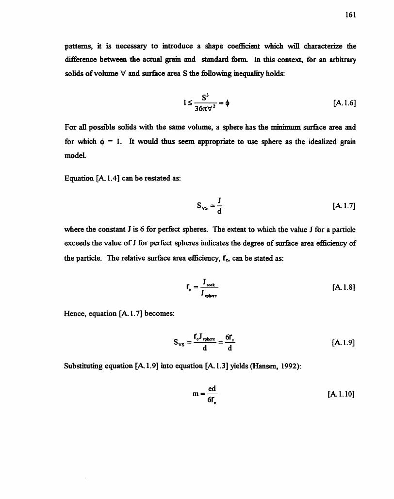
patterns, it is necessary to mtroduce a shape coefficient which wïii characterize the
difference between the acninl grain and standard f o m In this conte* for an arbiaary
solids of vohune V and surfàce area S the foilowing inequality holds:
For al1 possible soli& wirh the same volume, a sphere has the mmmium d c e area and
for which + = 1. It would thus seem appropriate to use sphere as the idealized grain
mode1
Equation [A 1.41 can be restated as:
where the constant J is 6 for perfect spheres. The extent to which the vahie J for a particle
exceeds the value of J for perfect spheres indicates the degree of surface area efficiency of
the particle. The relative surface area efficiency7 T, cm be stated as:
Hence, equation [A. 1.7 becomes:
Substituthg equation [A 1.93 mto equation [A 1.31 yields (Hansen, 1992):

Appendir 2
DERIVATION OF 1-D DYNAMIC EQUATION FOR
STEADY n o w THROUGH BURIED STREAMS
The total head, H, above a datum at any croswection of a buried stream, in geierai, cm
be represented by (Figure A2.1):
where:
z : vertical distance of the stream bed above datum,
d : depth of water measured perpendicularty fiom the water surface,
8 : bed dope angle,
a : khetic energy correction factor,
UV : velocity of flow through the void spaces of buried stream,
g : gravitational constant.
It is assumed that 0 and a are constant throughout the reach under consideration. T a b g
the stream bed as the x-axk and differentiating equation rA.2.11 with respect to length x
of the water surface profile, the following equation is obtained:


dd dy F o r d e , c o s h 1, d=y, and -=-
y : depth of water measured verticaily.
Thus, equation [A. 2.23 becomes:
It should be noted that the slope is defined as the sine of the slope angle and it is assumed
positive ifit descends in the direction of flow and negative ifit ascends. Unless energy is
added fiom outside to the flow, the fiction loss dH is a negative quanMy m the direction
of flow and the change in the bottom elewation dz is a negative quantity when the dope
descends.
Hence, fiction slope,
dz and dope of the channel bed, S, = --
dx
Substituthg these dopes m equation rA2.31:
a d =-UV- a du (u,) = -u- g h gn2 du

where:
U : bulk velocity = nUv
u d Substitutmg the expression for - - (ut) into equation [A2.5] yields:
2g dx
Aswming Q to be constant m the reach considered and dA = Tdy (where: T is the top
width)
Substituting equation rA.2.71 into equation IA2.61 yieids:
dy S a - % - -- - s o - Sf dx b- aUQT - ~ Q ' T
gn2A2 1--
@'A3
The t e m a m equation [A2.9] allows for n o n - d o m velocity distn'bution and has not
been established for r o c W . An assumption of a = 1 is within the accuracy which can be
expected (Stephenson, 1979). Therefore, equation rA2.91 becomes:
Let us denote the pore Froude number, k p as:

Substinrtmg equation [A2.11] into equation [A 1.101 yields:
Equation [A.2.12] is the general differential equation for gradua&-varied flow through
buied strearns under steady state condition, which demies the variation of the depth of
flow m a Stream of arbitrary shape with respect to longitudinal distance.

Appendix 3
CHARACTERIZING INDIVIDUAL PARTICLES
Table A.3.1 Dimensions of the rock particles dong a, b, and c axes.
Aris a (mm) 35.00 33.00 40.00 32.00 2 1.00 39.00 3 1-00 42.00 34.00 45.00 33.00 40.00 42.00 19.00 23.00 30.00 28.50 34.00 29.50 30.00 33.00 30.00 35.50 40.00 28.00 45.00 3 1.50 30.00 24.00 35.00 30.00
kxk b (mm) 19.00 23.00 2 1.00 2 1.00 17.00 17.00 20.00 29.00 21.00 22.00 16.00 12.00 23.00 15.00 21.00 16.00 20.00 26.00 20.00 15.00 27.00 13.00 15-00 16.00 25.00 20.00 17.00 28.00 23.00 21.50 19.00
Axh c (mm) 9.00 12.50 13.00 20.00 16.00 12.00 20.00 12.50 9.00 6.50 13.50 1 1.00 16.50 5.00 13.00 13.00 6.00 14.00 7.50 14.00 13.50 5.50 12.00 10.00 7.00 11-50 7.00 12.00 14.50 18.00 9.00

Table A.3.l (Contmued).

Table A3.1 (Continueci).


Appendix 5
DERIVATION OF EXPRESSION FOR
CEWITCAL REACH LENGTH (Lc)
The application of the energy equation between two adjacent sections of a buried stream
shown in Figure A 5.1 yields:
where:
S, : stream bed slope,
& : loss of head due to firidon,
y1 : depth of water at the downstream section,
y2 : depth of water at the upstream section,
UV* : void velocity at the downstream section,
Uvz : void velocity at the upstream section,
g : gravitationai constant,
L : Distance between the upstream and downstream section,
8 : Channel bed slope angle,
al : Kmetic energy correction fàctor for the downstream section,
al : Kmetic energy correction factor for the upstream section.
[AS. 11
The term a m equation [AS. 11 is used to correct the non-uaiformity of the velocity profle
across the cross-sections. For turbulent flow m open chameh with Sinple cro-sections
the value of a can be as low as 1.05. For non-Darcy flow through rock drains, it is
reasonable to assume a = 1.00, since uZvDg is very d and the deviation of the a a u a l


magnitude of a fkom imay does not affect significantly on the total magnitude of the tem
a ~ ~ ~ / 2 ~ . For ail practical pqoses, when the stream bed slope angle is s d l (ie., d e n 0
< 4 9 the vahie of cos 8 can be considered to be equal to one.
Therefore Smplincatioos Iike a = 1.00 and cos 9 = 1.00, wiü not violate the assumptions
of graduaüy-varied flow as stated m Section 2.3.1. Under such circu~llstances e q d o n
[A. 5.11 becomes:
The fiction loss term, &, m the right hand Sde of equation [A521 can be approximated b y:
where:
S f w : representative friction slope withm the reach considered.
One simple and efficient way of determinhg the magnitude of S, - is the arithmetic
average of Ectïon dopes at downstream and upstream sections, which yields:
Substitution of equation [A 5-41 mto equation [A 5.21 yields:
Differentiating equation [AS -51 with respect to downstream depth of flow, yl, yields:
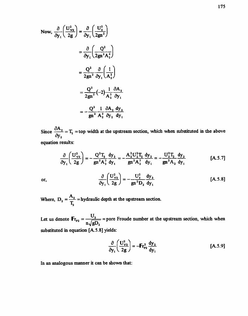
aA Smce 2 = '& =top width at the upstream section, which when substhted m the above
a y 2
equation results:
A, Where, D2 = - = hydraulic depth at the upstream section. T
Let us denote Fr, = U2 =pore Froude number at the upstream section, which d e n %/z substituted m equation [A. 5.81 yields:
In an analogous manner t can be shown that:

[AS. 101
For fidly-developed turbulent flow through rock drains, approhting fiction slope by
the Stephenson equation and differentiating the fiction slope term contained m the left
hand side of equation [A 5.51 wah respect to y1 yields:
Or,
Similarly it can be show that,
[A5 121
fA5.131
[AS. 141
[AS. 151
[A5 161
[AS. 191
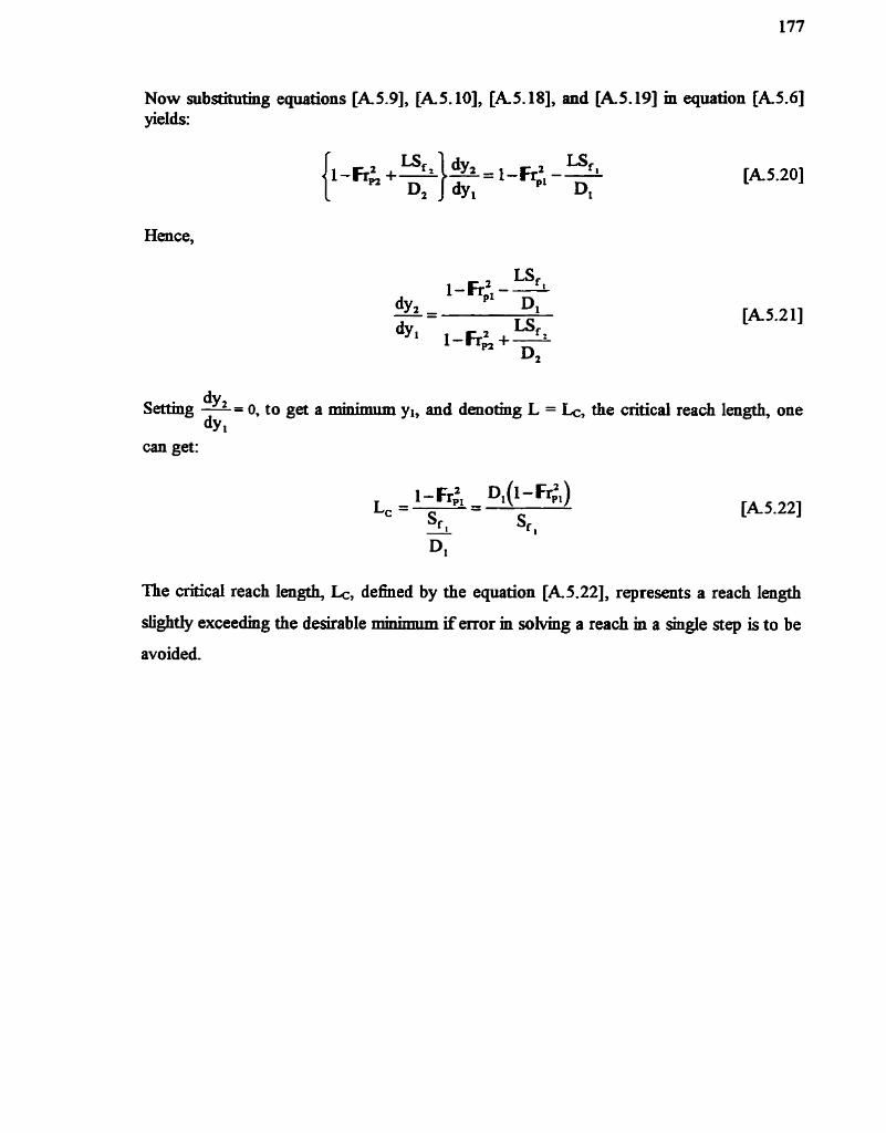
NOW substieutmg equations [A5.9], [A5.10], [A5.18], and [k5.19] m equation [A561 yields:
Hence,
can get:
The d c a l reach length, &, defined by the equation [A.5.22], represents a reach length
slightly exceednig the desirable mmmntm iferror m s o b g a reach in a Sngle step is to be
avoided-

Appendix 6
DERIVATION OF FIRST-ORDER
UNCERTAINTY EQUATIONS
A.6.1 Introduction
In order to iden* the components contnibuting to uncertainty m smnilated depths of a
non-Darcy flow, let us wnsider a rock dram of rectangular mss-section. The discharge
through such a rectangular drain can be computed as (when Wükms' equation is used):
where:
B : width of the rock drain.
Replacing the hydraulic mean radius, m, of equation LA6.11 by equation [2.6] yields:
Void ratio, e, and porosity, n, are related by the foiiowing eqilsition:
Replacing the void ratio of equation [A 6.21 by eqyation [A. 6.31 yields:

Solving equation [A 6-41 for depth of flow yields:
h an andogous way for fdly-developed turbulent flow, by ushg Stephenson's equation,
the expression for the depth of flow dong a rectanguiar rock drain can be deduced as:
The rnodels dweloped m Section 4.2 solves equation [A6.5] or [A6.6] for depths of
water at différent sections dong the rock drain, As there are no explicit çohitions of the
above two equations, an iterative numericd scherne was employed to sohe them When
Wilkins' equation is use& it cm be seen fiom equation 1416.51 that the depth of flow at
any section of a rectangular rock dram is a fimction of swen mdependent variables,
nameiy: drain width, discharge, Wilkins' constant, shape coefficient, particle diameter,
Ection dope, and porosity. Similariy, when Stephenson's equation is useci, it can be seen
fkom equation LA.6.61 that the depths of flow through a rectanguiar rock drain are
fùnctions of six mdependent variables: drain width, discharge, fiction factor, particle
diameter, fiction dope, and porosity. Therefore, uncertain@ m determinmg the exact
magnitude of these independent variables will resuh m an erroneous simulated water
surface profiles through rock drain.
Average depth of water through buried streams can be computed by applymg the first-
order uncertainty equation, equation [2.30] to equation [A6.5] and [A 6-61, which yields:
[A. 6.71
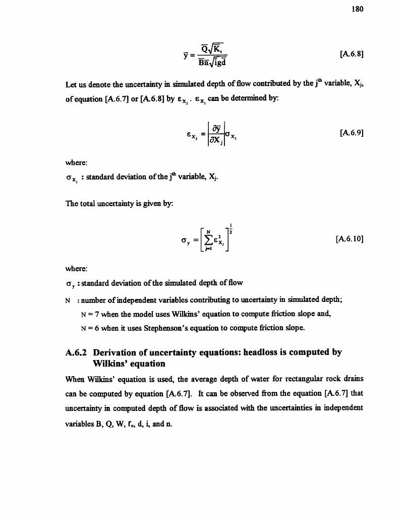
Let us denote the uncertainty in simulated depth of flow conmiuted by the j' variable, Xj,
of equation [A6.71 or [A631 by sXj . E,, can be d e t d e d by
- Exj -
where:
Ox. : standard daiation of the j" variable, Xj.
The total uncertahy is &en by:
where:
o, : standard dwiation of the sinnilated depth of flow
N : number of independent variables contributing to uncertahty m simulated depth;
N = 7 when the model uses Wilkins' equation to compute fiction slope and,
N = 6 when it uses Stephenson's equation to compute Fiction slope.
A.6.2 Derivation of uncertainty equations: headloss is computed by Wilkinsy equation
When Wilkms' equation is use& the average depth of water for rectangular rock drains
can be computed by eqyation rA.6.71. It cm be observed fiom the equation [A6.71 that
uncertainty in computed depth of flow is associated with the uncertamties in independent
variables B, Q, W, re, d, i, and n.

() Contribution of&ain widih to uncerîainty in simulated depth
The contribution of drain width to the uncertahty Ùt the computed depth of flow can be
determined fiom the fonowing equation:
where:
E : uncertainty m computed depth due to drain width,
a~ : standard deMation of the drain width.
Substitution of equation [k6.71 mto equation [k6.11] yields:
where:
CVe : coefficient of variation of drain width = 2. B
ci) Contribution of dischaqge to uncertuinty in simulated depth
The uncertainty in sirmilated depth of flow due to the uncertainty m discharge is given by:
where:

B : mcertainty m computed depth due to discharge
a, : standard deviation of the measured discharge.
Substitution of eqyation [A 6.73 into eqyation [A6.16] yields:
where:
=Q CVQ : coefficient of variation of discharge = -=- . Q
(iiq Contribution of shape coeflikient to uncertain$ in simrlated depth
The uncextainty m smnrlated depth of fiow due to the uncertahty m shape coefficient is
given by:
where:
: uncertainty m computed depth due to shape coefficient,
a, : standard devhtion of the shape coefficient.
Substitution of equation [A 6.73 mto equation [A 6.2 11 yields:

where:
CV, : coefficient of variation of r. =S. r*
(iV) Contribution of Mikins' constant to uncertainty in simuiated deprih
The uncertahty m Smulated depth of flow due to the uncertainv m Wiikms' constant is
given by:
where:
cw : uncex-tBmty m computed depth due to Wilkms constant,
G~ : standard deviation of Wilkins constant.
Substitution of eqyation [k6 .6 ] mto equation [A6.25] yields:

where:
CVw : coefficient of variation of WiIkms constant =% W'
(v) Contribution of pamkIe diameter to uncmîainty in sirnul& depth
The uncertainty m sùmdated depth of flow due to the mcertainty m particle diameter is
&en by.
where:
sd : uncertainty m computed depth due to particle diameter,
O* : standard deviation of particle diameter.
Substitution of equation [A 6.71 mto equation [A 6.291 yields:
where:
cd : unceftainty m computed depth due to partide diameter,
CVd : coefficient of variation of particle diameter =% . d
(vi) Contribution offiction dope to uncertainty in simulated depth
Uncertamty (U,) m gmulated depth of flow due to the uncertainty m hydraulic gradient is

wfiere:
s i : mcertainty m computed depth due to fiction dope,
oi : standard deviation of computed hydraulic gradient.
Substitution of equation IA6.71 mto equation [A 6.331 yields:
CVi : coefficient of variation of hydradic gradient =% . i
(vii) Contributio~ of porosity to uncertuinty in simulated depth
The uncertainty in Smulated depth of flow due to the uncertahty in porosity is &en by:
where:
E, : uncertamty m computed depth due to porosity,
un : standard deviation of the estimated porosity.
Squaring both sides of eqyation [A 6.71 yields:

Merentiating equation [A6.38] wiîh respect to porosity, n, yie1ds:
From equation [A6.37l, uncertahty due to porogty,
or,
where:
[A. 6-42]
n4 on E, = 0 . 5 0 ~ --- -- in'. i3]@-S) E [A.. 6.441

-6, CV. : coefficient of variation of porosty -y. n
A.6.3 Derivation of uncertainty equations: headloss is computed by Stephenson's equation
By using the Stephenson equation, the average depth of water through a rectangular rock
drain can be computed by eqyation IA6.71. It can be observed fiom equation [A6.71 that
the uncertainty m computed depth of flow is associated with the uncertainty m
independent variables B, Q Ki, n, i, and d.
(i) Contribution of drain widtk to unceriuinty in simulated dqth
The contribution of drain width to the uncertainv in the computed depth of flow can be
detedned fiom the foIlowing equation:
Substitution of equation [A6.8] hto equation [A6.47] yields:

GU) Conbibutiun of discliagc tu uttcertcu'ng UI simdated dqth
The mcertainty in computed depth of fîow due to the uncertamty m discharge is &en by:
SubsMuting equation [A6.8] into equation IA6.521 yields:
(iii) Coninbution offnctrgon coeflcient to uncertainty in simuluted depth
The uncertahty m sirmilated depth of flow due to the uncertainty m Stephenson constant
is &en by:
where:
e : uncertainty m computed depth due to Stephenson friction factor,
O 4 : standard deviation of fiction fàctor.
Substituthg equation [A. 6.8 ] mt O equation [A. 6.5 61 yields:

- 65 CVy : coefficient of variation of the Stephawn's constant -- . Kt
(iv) Conbibutiun offn'crion dope to uncertainty in simirlated dq th
The uncertainty m simuiated depth of flow due to the uncertamty in fiction dope is given
by:
Subdtuting equation [A 6.81 mto equation [A. 6.601 yields:
[A. 6.601
(v) Contribution of particte diameter to uncertainîy in simuluted depth
The uncertainty m Smulated depth of flow due to the unceriahty in particle diameter is
@en by:
Substihmng equation rk6.81 mto equation [A6.64] yields:

(vi) Conaibution of pmosity to uncafainty in simulotc dqth
The uncertahty in Similated depth of flow due to the uncertainty m porosity is @en by
Substituthg eqyation [A 6.81 mto equation [A 6.681 yields:

IMAbt LVALUAI IUN TEST TARGET (QA-3)
APPLIED il IMAGE. lnc - .-- 1653 East Main Street - -. , Rochester. NY 14609 USA -- --= Phone: 71 61482-0300 -- -- - - Fa : 71 61288-5989
O t993. Applied Image. lm.. Ail RighQ Reserved