Flight Test Bed for Visual Tracking of Small UAVs

Lili Ma, Vahram Stepanyan, Chengyu Cao, Imraan Faruque,

Craig Woolsey and Naira Hovakimyan

Dept. of Aerospace and Ocean Engineering, Virginia Tech, Blacksburg, VA 24061, USA.

This paper describes the development of an unmanned aerial vehicle (UAV) system,which will be used to demonstrate multiple-vehicle flight control algorithms. Planneddemonstrations include vehicle coordination experiments involving autonomous air, ground,and marine vehicles. More immediately, a system of two UAVs will be used to demonstrateadaptive visual tracking algorithms. To speed development time, critical hardware such asthe aircraft autopilots and self-stabilizing gimballed camera system are purchased commer-cially. These systems are being installed in a commonly available hobby industry airframe.This paper describes component selection and high-level integration and results from earlyflight tests. The paper also describes the vision-based target tracking algorithm to bedemonstrated using this system.

I. Introduction

Military and civilian applications of unmanned air vehicles (UAVs) have dramatically increased in recentyears. Within the spectrum of existing UAVs, small, low-cost vehicles are finding use in a number of

niche applications. Small UAVs are especially appealing for use in research projects focused on autonomousvehicle coordination because they are inexpensive to build and repair. Moreover, there are highly capable,commercially available autopilots which can transform an ordinary radio control (R/C) aircraft into a sophis-ticated flight control system test bed. Experimental systems play a crucial role in validating newly developedcontrol algorithms. This paper describes a UAV system developed by the Virginia Center for AutonomousSystems (VaCAS) at Virginia Tech. While the system was developed with a view toward flexibility, antici-pating a wide range of possible applications, an immediate objective is to implement the vision-based targettracking guidance algorithms described in Refs. 1–4. We note that these algorithms couple estimation andcontrol to achieve the control objective. Separately, an alternative control algorithm is developed at VaCASthat assumes a custom-built gimbal for the camera, the open-loop control of which enables decoupling ofestimation from feedback control 5.

Development of the VaCAS UAV system was guided, in part, by similar UAV systems developed at theNaval Postgraduate School (NPS) and Brigham Young University (BYU). The rapid flight test prototypingsystem developed by NPS, as documented in Refs. 6, 7, has served as the primary model for the VaCASUAV system. The NPS system includes: 1) a commercial off-the-shelf (COTS) autopilot system, the Piccoloautopilot from Cloud Cap Technology 8, 2) a ground control system for UAV guidance and navigation, 3)an on-board camera with a custom pan-tilt unit driven from the ground station, and 4) a COTS imageprocessing software package, called PerceptiVU 9, running on a separate ground computer. Video from theonboard camera is transmitted to the ground using a 2.4 GHz wireless data link. A 900 MHz telemetrylink operates between the autopilot and the ground control station. Development of serial communicationinterfaces is documented in Ref. 10. More details about the system setup can be found in Refs. 6, 7.

The UAV test bed developed at the MAGICC Lab at BYU is quite similar to the NPS system. TheBYU system was also developed with a view toward cooperative control experiments involving multiple vehi-cles 11,12. The setup includes components similar to the four described above for the NPS system, althoughMAGICC Lab researchers developed most of these components in-house. Developing custom hardware andsoftware gives researchers more freedom to develop and implement control algorithms and, in some cases,may lead to new commercial products. On the other hand, it takes considerable time and breadth of ex-pertise. In developing a UAV system for VaCAS, the research objectives and project time-line imposeda trade-off between system flexibility and rapid development. Ultimately, it was decided that the VaCAS

1 of 10

American Institute of Aeronautics and Astronautics

AIAA Guidance, Navigation, and Control Conference and Exhibit21 - 24 August 2006, Keystone, Colorado

AIAA 2006-6609

Copyright © 2006 by the American Institute of Aeronautics and Astronautics, Inc. All rights reserved.

system should include a COTS autopilot system and gimballed camera system. Image processing softwareis being developed in-house.

The paper is organized as follows. In Section II, we describe the system hardware and software andinclude data from preliminary test flights. Section III formulates a specific vision-based UAV trackingproblem; the control algorithm is presented in Section IV. Simulation results are described in Section V. Wegive concluding remarks and describe plans for continuing work in Section VI.

II. Test Bed

Vision-based air-to-air tracking experiments are scheduled for fall 2006. At time of writing, all majorcomponents of the UAV test bed have been selected and most of these components have been purchased andintegrated. This section describes the ongoing development effort, starting with an overview of the systemarchitecture and followed by a more detailed discussion of each key component.

II.A. Overview of the System Architecture

Observing a trade-off between ease of development and system flexibility, we have chosen to purchase COTShardware, including the airframe, autopilot system, and gimballed vision system. The architecture will besimilar to the NPS setup described in Refs. 6, 7, but possibly with a single ground station performing bothUAV guidance and navigation tasks and image processing functions. The architecture is shown in Figure 1.A modified R/C scale fix-wing aircraft houses an autopilot and a gimballed camera as its primary payloads.Video from the onboard camera is transmitted to the ground station for processing via a 2.4 GHz wirelesslink. Images are processed on the ground station, generating essential information about the target, suchas its centroid and estimated dimensions. This information is passed to the the guidance and navigationmodule, which then calculates the desired aircraft trajectory. The appropriate guidance commands arepassed to the UAV through a ground-based telemetry and control system purchased with the autopilot.The servo-actuated gimbal for the video camera is automatically adjusted from the ground based on locallycomputed information about the relative motion of the target with respect to the follower. The gimbal iscontrolled through a separate communication channel which is independent of the autopilot system. Forsafety, the autopilot system allows a human supervisor to intervene and take manual control of the vehicle.

Gimbaled Camera

2.4 GHz Video Link Gimbal Commands

Piccolo Autopilot

Piccolo Manual Control Piccolo Ground Station

Operator Interface

Ground Station

Serial Link

900 MHz Piccolo Protocol

Full duplex serial Full duplex serial

Figure 1. Flight test setup.

If early field tests indicate that the image processing algorithms are too computationally expensive to beimplemented along with the control algorithm in a single computer, the configuration shown in Figure 1 canbe easily modified to include a separate ground-based image-processing computer. Outputs from the imageprocessing module can be provided to the control module through direct ethernet or serial link.

II.B. Airframe and Propulsion

The aerial vehicle is built around a commercial R/C airframe known as the Sig Rascal 110. This is a high-wing, box-fuselage aircraft with a wing span of 110 inches. The airframe is pictured in Figure 2. Thisairframe was selected for several reasons, but chiefly for its size and payload capability. The Rascal 110 isone of the largest R/C airplanes available. With the standard R/C configuration weight of approximately

2 of 10

American Institute of Aeronautics and Astronautics

13 to 14 pounds (depending on the amount of fuel remaining in the tank), the aircraft has a wing loading ofonly 19 to 22 oz/ft2, which is reflected by its relatively slow flight. Because it is so large, the dynamic modesare significantly slower than those of a smaller UAV, a fact which is advantageous for control algorithmsthat require extensive processing.

Figure 2. Sig Rascal 110 base airframe.

Model airplanes and many small UAVs are normally powered by a mixture of methanol (70 ∼ 90% byvolume), nitromethane (2 ∼ 15% by volume), and castor oil (18 ∼ 23% by volume). These engines are knownas “glow engines” because a glow plug is used to ignite the mixture. The fuel consumption is relatively high,however. For this airframe and payload, the aircraft would be required to carry significant fuel reserves orwould be constrained to short flight durations. To circumvent this problem for aircraft of this size, manyR/C pilots use small gasoline “chainsaw-type” engines . These engines have a longer runtime, but are slightlyheavier and use a spark plug-based ignition system that can create radio interference.

A less common propulsion method involves using diesel fuel. Although two-stroke diesel engines can bemessy, they boast a high torque output and no spark or glow plugs. One may typically use an engine with2/3 the displacement of a comparable glow or gasoline engine, significantly reducing weight. The UAVs inthe test bed described here use an OS MAX engine with a 1.08 in3 displacement. The engine is actually aglow engine which has been converted to use diesel fuel by swapping the standard head for one manufacturedby Davis Diesel Development 13. The converted engine generates ample power with a significantly reducedpropulsion system weight. An additional advantage is that diesel engines are less sensitive to back pressure,which allows the exhaust to be ducted through the interior of the airplane and vented out the tail. Sincetwo-stroke engines (whether, glow, gasoline, or diesel) normally vent a significant amount of oil throughtheir exhaust, there is a tremendous advantage to locating the engine exhaust downstream of sensors andactuators, particularly a gimballed video system.

II.C. Avionics

Cloud Cap Technology’s Piccolo Plus avionics suite was selected as the onboard autopilot. The systemcomprises a vehicle-mounted computer and sensor suite and a ground station which provides GPS positioncorrection and a user interface. The on-board unit is highly integrated, combining three angular rate gyros,three accelerometers, a GPS unit, pitot/static air pressure sensors, a 40 MHz PowerPC processor, and a UHFdata modem in a ruggedized enclosure. The manufacturer also makes its autopilot source code available forpurchase, allowing a user to load a newly developed controller in place of the factory-supplied controller.

At the time of writing, the avionics package has been integrated into the airframe and motion data havebeen collected for several manual and autonomous flights in order to verify the sensing system’s accuracy.Figure 3 shows plots of data logs, including 3-D position, from GPS, pressure and GPS altitude, airspeedand acceleration. The simple test flight included a takeoff, downwind leg, and landing. Significant events(such as take-off and landing) are obvious from the data. The data in Figure 3 (a) were taken from theonboard GPS receiver. Latitude/longitude data were converted to a local right-handed (East-North-up)coordinate frame with distances measured in feet from the starting location. In Figure 3 (b), two altitudeplots are shown; one is based on static pressure, relative to the standard atmosphere, while the other is GPS-measured altitude. The plot illustrates the inherent noise in GPS altitude measurements, but the trends showreasonable agreement. Altitude measurements are Kalman filtered with a much higher degree of confidencein barometric altitude (i.e., low noise covariance) as compared with GPS. The coarse GPS altitude readingsare therefore not a significant performance handicap. Having demonstrated the sensing system’s accuracy,a careful, well-planned procedure is now being followed to transition the UAV to autonomous flight.

Earlier it was mentioned that this aircraft flies slowly in comparison to smaller, more common R/Caircraft. The airspeed plot in Figure 3 (c) shows an average airspeed of approximately 9 m/s (roughly 20mph). Figure 3 (d) shows the recorded accelerometer data, expressed in traditional body-fixed stability axes.

3 of 10

American Institute of Aeronautics and Astronautics

−400

−300

−200

−100

0

100

−100

0

100

200

300

1950

2000

2050

FeetFeet

Alti

tude

, ft

(a) 3-D trajectory

0 10 20 30 40 50 60 70580

590

600

610

620

630

640

Time, seconds

Alt

abov

e S

L, m

eter

s

Altitude above SL with respect to time

Pressure AltitudeGPS Altitude

(b) Altitude

0 10 20 30 40 50 60 70−2

0

2

4

6

8

10

12

14

Time, seconds

TA

S[m

/s]

Airspeed wrt time

(c) Airspeed

0 10 20 30 40 50 60 70−30

−20

−10

0

10

20

30

40

Time, seconds

Acc

eler

atio

n, m

/s2

Accelerometer measurements

X accelerometerY accelerometerZ accelerometerTotal

(d) Accelerometer

Figure 3. Data logs for an example flight.

These flight data were collected before all of the sensors were zeroed; a steady state bias was removed duringpost-processing for the data shown in Figure 3 (c).

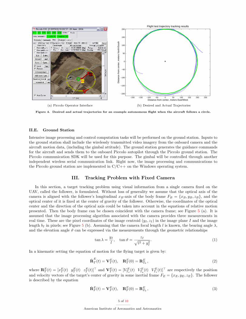
Multiple autonomous flights have also been achieved on a day-to-day basis, where the given flight planshave included circles, rectangles, and user-specified way points. Figure 4 (a) shows a screen shot of thePiccolo operator interface during one example autonomous flight when the aircraft follows a circle, wherethe small green circle indicates the location of the ground station, the number “99” indicates the center ofthe circle, and the vector from “99” to “98” shows the radius of the circle. The desired trajectory is shownvia the yellow circle. The red arrow indicates the position of the aircraft at the time of the screen shot.Figure 4 (b) shows the desired and actual trajectories with the desired trajectory plotted in green and theactual plotted in blue.

II.D. Onboard Vision System

To save time and effort in developing the test bed, we have focused on purchasing COTS gimbal products.The search for small, light-weight, automatically stabilized gimbal systems led to three viable options:the Controp D-STAMP 14, the Tenix 15, and the Cloud Cap Technology TASE gimbal systems 16. Aftercomparing features and cost, it was determined that the Cloud Cap system best suits the needs of thisproject. The device is expected to become commercially available in late summer 2006. The Cloud CapTASE gimbal is designed to have an overall package size of 5× 4× 7 inches. It weighs less than 1Kg and has360◦ continuous azimuth and 23◦-up and 203◦-down tilt. The gimbal will be controlled through a stand-aloneserial communication link (using wireless modems), which is independent of the Piccolo autopilot link usedfor motion data telemetry and for guidance and navigation. At the same time, to progress in our project,several Black Widow AV 600mw Brown Bag Kits 17 have been purchased, and one has been installed/fixedon the aircraft for computer vision algorithm development.

4 of 10

American Institute of Aeronautics and Astronautics

(a) Piccolo Operator Interface

−200 −150 −100 −50 0 50 100 150 200 250

−200

−150

−100

−50

0

50

100

150

200

Distance from center, meters East/West

Dis

tanc

e fr

om c

ente

r, m

eter

s N

orth

/Sou

th

Flight test trajectory tracking results

(b) Desired and Actual Trajectories

Figure 4. Desired and actual trajectories for an example autonomous flight when the aircraft follows a circle.

II.E. Ground Station

Intensive image processing and control computation tasks will be performed on the ground station. Inputs tothe ground station shall include the wirelessly transmitted video imagery from the onboard camera and theaircraft motion data, (including the gimbal attitude). The ground station generates the guidance commandsfor the aircraft and sends them to the onboard Piccolo autopilot through the Piccolo ground station. ThePiccolo communication SDK will be used for this purpose. The gimbal will be controlled through anotherindependent wireless serial communication link. Right now, the image processing and communications tothe Piccolo ground station are implemented in C/C++ on the Windows operating system.

III. Tracking Problem with Fixed Camera

In this section, a target tracking problem using visual information from a single camera fixed on theUAV, called the follower, is formulated. Without loss of generality we assume that the optical axis of thecamera is aligned with the follower’s longitudinal xB-axis of the body frame FB = {xB , yB , zB}, and theoptical center of it is fixed at the center of gravity of the follower. Otherwise, the coordinates of the opticalcenter and the direction of the optical axis could be taken into account in the equations of relative motionpresented. Then the body frame can be chosen coincident with the camera frame; see Figure 5 (a). It isassumed that the image processing algorithm associated with the camera provides three measurements inreal time. These are the pixel coordinates of the image centroid (yI , zI) in the image plane I and the imagelength bI in pixels; see Figure 5 (b). Assuming that the camera focal length l is known, the bearing angle λ,and the elevation angle ϑ can be expressed via the measurements through the geometric relationships

tanλ =yI

l, tanϑ =

zI√l2 + y2

I

. (1)

In a kinematic setting the equation of motion for the flying target is given by:

RE

T (t) = VET (t), RE

T (0) = RET0

, (2)

where RET (t) = [xE

T (t) yET (t) zE

T (t)]> and VET (t) = [V E

Tx(t) V E

Ty(t) V E

Tz(t)]> are respectively the position

and velocity vectors of the target’s center of gravity in some inertial frame FE = {xE , yE , zE}. The followeris described by the equation

REF (t) = VE

F (t), REF (0) = RE

F0, (3)

5 of 10

American Institute of Aeronautics and Astronautics

where REF (t) = [xE

F (t) yEF (t) zE

F (t)]> and VEF (t) = [V E

Fx(t) V E

Fy(t) V E

Fz(t)]> are respectively the follower’s

position and velocity vectors in the same inertial frame FE .We assume that the follower can measure its own states in addition to the visual measurements, but does

not have any knowledge about the target’s size or state, other than the camera image. The target’s relativeposition with respect to the follower is given by the inertial vector

RE = RET −RE

F , (4)

and the relative motion is:

RE(t) = VET (t)−VE

F (t), RE(0) = R0 , (5)

where the initial condition is given by RE0 = RE

T0−RE

F0. The objective is to find a guidance law VE

F (t) forthe follower in order to maintain a pre-specified relative position described by Rc(t), λc(t), ϑc(t) given inthe body frame FB . This is a challenging control problem, since the relative range R(t) = ‖RE(t)‖ is notmeasured directly. It is related to the image plane measurements (yI(t), zI(t), bI(t)) via the equation

R =b

bI

√l2 + y2

I + z2I

∆= baI . (6)

Here b > 0 is the size of the target that is assumed to be constant but otherwise unknown to the follower.

(a) Coordinate frames and angles definition (b) Camera frame and measurements

Figure 5. Coordinate illustrations.

It is worth noting that the dynamic equation (5) is written in the inertial frame FE , the referencecommands Rc(t), λc(t), ϑc(t) are given in the body frame FB and the visual measurements are taken inthe image plane. To unify all the quantities of interest we introduce the scaled relative position vectorrE(t) = RE(t)

b , the dynamics of which are written as

rE(t) =1b

[VE

T (t)−VEF (t)

], rE(0) = rE

0 , (7)

where rE0 = RE

0b . Using the coordinate transformation matrix LFB/E from the inertial frame FE to the body

frame FB , we can write rE = LF>B/ErB , where components of rB are related to the visual measurements viathe following algebraic expressions:

rBx = aI cos ϑ cos λ,

rBy = aI cos ϑ sinλ,

rBz = −aI sinϑ . (8)

Hence the vector rE is available for feedback. Similarly, the reference commands Rc(t), λc(t), ϑc(t) can betranslated to the inertial frame as rE

xc(t)rEyc(t)

rEzc(t)

=Rc(t)b(t)

L>B/E

cos ϑc(t) cos λc(t)cos ϑc(t) sinλc(t)

− sinϑc(t)

, (9)

6 of 10

American Institute of Aeronautics and Astronautics

Here we notice that for the given bounded commands Rc(t), λc(t) and ϑc(t) the reference vector ξc =[ rE

xc(t) rEyc(t) rE

zc(t) ]> is bounded.The problem is reduced to designing a guidance command u(t) = VE

F (t) for the follower, using theavailable signal ξ(t) = rE(t), such that the trajectories of the system

ξ(t) =1b[−u(t) + VE

T (t)] , (10)

asymptotically track the bounded reference command ξc, regardless of the realization of the target’s motion.Thus we have a simultaneous tracking and disturbance rejection problem for a multi-input multi-output linearsystem (10), with positive but unknown high frequency gain in each control channel, that has to be solvedfor a reference signal ξc(t) that depends on the unknown parameter b via the expressions in equation (9).

IV. Guidance Law

The problem formulated above has been solved in Ref. 4 when the target’s velocity is subject to thefollowing assumption.

Assumption 1 Assume that the target’s inertial velocity VET (t) is a bounded function of time and has

bounded time derivative, i.e. VET (t), VE

T (t) ∈ L∞. Further, assume that any maneuver made by the target issuch that the velocity returns to some constant value in finite time or asymptotically in infinite time with arate sufficient for the integral of the magnitude of velocity change to be finite, that is VE

T (t) = Vs +∆VT (t),where Vs is a constant and ∆VT (t) ∈ L2.

Since b is a constant, this assumption can be formulated for the function d(t) = 1b(t)V

ET (t) as follows:

d(t) = ds + δ(t) , (11)

where ds ∈ R3 is an unknown but otherwise constant vector, and δ(t) ∈ L2 is an unknown time-varyingterm. Applying the corollary of Barbalat’s lemma from Ref. 18 (p.19), we conclude that

δ(t) → 0, t →∞ . (12)

It is interesting to notice that obstacle avoidance maneuvers by the target verify this assumption, providedthat after the maneuvers the target velocity returns to a constant in finite time or asymptotically in infinitetime subject to L2 constraint. The guidance law derived in Ref. 4 is given by the equation

u(t) = b(t)g(t)

g(t) = ke(t) + d(t)− ˙ξc(t)

˙b(t) = σProj(b(t), e>(t)g(t)), b(t0) = b0 > 0˙d(t) = GProj(d(t), e(t)), d(t0) = d0 , (13)

where e(t) = ξ(t)−ξc(t) ∈ R3 is the tracking error, b(t) ∈ R and d(t) ∈ R3 are the estimates of the unknownparameter b and the nominal disturbance d respectively, k > 1/4, σ > 0 are constants (adaptation gain), Gis a positive definite matrix (adaptation gain), and Proj(·, ·) is the Projection operator 19, that guaranteesknown conservative bounds 0 < bmin ≤ b(t) ≤ bmax, and ‖d(t)‖ ≤ d∗. In equation (13), ξc is the estimatedreference command given by

ξc =

ξcx(t)ξcy(t)ξcz(t)

=Rc(t)

b(t)

cos(ϑc(t)) cos(λc(t))cos(ϑc(t)) sin(λc(t))

− sin(ϑc(t))

. (14)

The guidance law u(t) in equation (13) guarantees asymptotic tracking of the reference trajectory ξc(t). Ithas been shown that in the case of formation flight with constant commands Rc, λc, ϑc the true referencecommand ξc(t) is guaranteed to be tracked asymptotically in the presence of the excitation signal thatis added to relative range command Rc, when also the parameter estimates converge to the true values.

7 of 10

American Institute of Aeronautics and Astronautics

The amplitude of the excitation signal can be controlled according to the intelligent excitation techniqueintroduced in Ref. 1. It is done by choosing the amplitude dependent upon tracking error. Below insimulations we incorporate this technique to ensure parameter convergence.

In the case of target interception, parameter convergence is not required since the reference command isξc(t) = ξc(t) = 0. Therefore, the guidance law u(t) in equation (13) always guarantees target interception.

V. Simulation

In simulations, the tracking error is formed by using aI and angles λ, ϑ that relate to the measurements(yI(t), zI(t), bI(t)) via the equations (1) and (6). The reference command is formulated according toequation (14), where the signal b(t) is generated according to the adaptive law in equation (13) with theinitial estimation of b(0) = 1.5ft. The excitation signal is introduced following Ref. 1 with the followingamplitude:

a(t) =

k1, t ∈ [0, T )

min{k2

∫ t

t−Te>(τ)e(τ)dτ, k1 − k3}+ k3, t ≥ T ,

where e(t) is the tracking error, T = 2πω is the period of the excitation signal a(t) sin(ωt), ki > 0, i = 1, 2, 3

are design constants set to T = 3sec, k1 = 0.4, k2 = 500, k3 = 0.0002. In the simulation scenario a targetof length b = 3ft starts moving with the constant velocity VTx = 30ft/sec, VTy = VTz = 0 and follows thevelocity profile displayed in Figure 7 (b) (the analytic expressions are not presented). The target’s velocitycan be represented as VT (t) = b(d+ d(t)), where d = [10 0 0]>ft/sec is a constant term and d(t) is a time-varying term that captures all the maneuvers and the asymptotically decaying perturbations and satisfiesthe inequalities ‖d(t)‖∞ ≤ 40, ‖ ˙d(t)‖∞ ≤ 7.5π and d(t) ∈ L2. We recall that ˙d(t) represents the targetacceleration, and, hence, during the maneuvers it is bounded. The follower is commanded to maintain arelative range of Rc = 15ft, bearing angle of λc = 15o and relative elevation of ϑc = 0o. Initial conditionsare chosen to be xB0 = 36ft, yB0 = 21ft, zB0 = −15ft. The guidance law is implemented accordingto equation (13) with k = 3.5. Simulation results are shown in Figures 6, 7, and 8. Figure 6 shows thesystem output convergence, where (b) is the zoomed version of the tracking performance over a time periodwhen excitation is active. The parameter convergence is shown in Figure 7 (a). Figure 7 (b) shows thatthe guidance law is able to capture the target’s velocity profile with a certain lag, which disappears whenthe target returns to the nominal velocity. The large fluctuations in the estimation of d0 are due to thepresence of target acceleration during the maneuvers. We note that the magnitude of the velocity varies in[−40 40]ft/sec. The target’s size estimation gradually converges to the true value. The range discrepancyis visible only during the target’s maneuvers and vanishes as the target returns to its nominal motion. Thebearing angle has big fluctuations due to the target’s turning maneuvers, which are assumed to stay in thefield of view of the aerial vehicle during the entire task. Figure 8 demonstrates the amplitude of intelligentexcitation. As it can be seen from the figure, excitation is activated only during the target maneuvers andvanishes as the target returns to its nominal motion.

VI. Concluding Remarks

An automated vision-based target tracking system is introduced. The flight test bed is still being devel-oped; data from preliminary flight tests are included here. This flexible UAV system test bed will provide theability to implement and test a variety of UAV flight control tasks, including multiple-vehicle coordinationexperiments and vision-based flight control. Experiments involving autonomous visual tracking of manuallypiloted UAV are ongoing. The vision-based target tracking algorithm that will be implemented was firstpresented in an earlier paper, but is revisited here, along with new simulation results illustrating its viability.Of course, the algorithm can not be directly implemented as presented because the camera is assumed to befixed with respect to the airframe. Ongoing efforts include the adaptation of the visual tracking algorithmpresented here to a camera which is mounted on a servo-actuated 2-axis gimbal.

8 of 10

American Institute of Aeronautics and Astronautics

0 10 20 30 40 50 600

20

40

60Outputs, R in ft, λ and θ in deg

0 10 20 30 40 50 60−20

0

20

40

0 10 20 30 40 50 60−40

−20

0

20

40

t

R(t)R

c(t)

Λ(t)Λ

c(t)

Θ(t)Θ

c(t)

(a) Outputs convergence

18 20 22 24 26 28 30 32 34 3624

25

26

27Outputs, R in ft, λ and θ in deg

18 20 22 24 26 28 30 32 34 3610

12

14

16

18

18 20 22 24 26 28 30 32 34 36−2

−1

0

1

2

t

Θ(t)Θ

c(t)

Λ(t)Λ

c(t)

R(t)R

c(t)

(b) Zoomed output tracking

Figure 6. System output convergence.

Acknowledgments

The authors gratefully acknowledge the advice and guidance of V. Dobrokhodov of NPS. This work wassponsored in part by ONR Grant #N00014-05-1-0828 and AFOSR MURI subcontract F49620-03-1-0401.

References

1Cao, C. and Hovakimyan, N., “Vision-Based Aerial Tracking Using Intelligent Excitation,” American Control Conference,Portland, OR, USA, June 8-10 2005, pp. 5091–5096.

2Cao, C. and Hovakimyan, N., “Vision-Based Aerial Tracking using Intelligent Excitation,” Submitted to Automatica,2005.

3Stepanyan, V. and Hovakimyan, N., “A Guidance Law for Visual Tracking of a Maneuvering Target,” American ControlConference, Minneapolis, Minnesota, June 14-16 2006, pp. 2850–2855.

4Stepanyan, V. and Hovakimyan, N., “Adaptive Disturbance Rejection Guidance Law for Visual Tracking of a ManeuveringTarget,” AIAA Guidance, Navigation, and Control Conference and Exhibit , San Francisco, CA, Aug. 15-18 2005.

5Cao, C., Hovakimyan, N., and Evers, J., “Active Control of Visual Sensor for Aerial Tracking,” AIAA Guidance, Navi-gation, and Control Conference and Exhibit , Keystone, Colorado, USA, Aug. 21-24 2006.

6Wang, I. H., Dobrokhodov, V. N., Kaminer, I. I., and Jones, K. D., “On Vision-Based Target Tracking and RangeEstimation for Small UAVs,” AIAA Guidance, Navigation, and Control Conference and Exhibit , San Francisco, CA, Aug.15-18 2005.

7Kaminer, I. I., Yakimenko, O. A., Dobrokhodov, V. N., and Jones, K. D., “Rapid Flight Test Prototyping System andthe Fleet of UAV’s and MAVs at the Naval Postgraduate School,” AIAA 3rd “Unmanned Unlimited” Technical Conference,Workshop and Exhibit , Chicago, Illinois, Sep. 20-23 2004.

8“Cloud Cap Piccolo,” http://www.cloudcaptech.com/piccolo.htm.9“PerceptiVU,” http://www.perceptivu.com/.

10Dobrokhodov, V. and Lizarrage, M., “Developing Serial Communication Interfaces for Rapid Prototyping of Navigationand Control Tasks,” AIAA Modeling and Simulation Technologies Conference and Exhibit , San Francisco, CA, Aug. 15-182005.

11Quigley, M., Goodrich, M. A., Griffiths, S., Eldredge, A., and Beard, R. W., “Target Acquisition, Localization, andSurveillance using a Fixed-Wing Mini-UAV and Gimbaled Camera,” IEEE International Conference on Robotics and Automa-tion, Barcelona, Spain, Apirl 18-22 2005.

12McLain, T. and Beard, R., “Unmanned Air Vehicle Testbed for Cooperative Control Experiments,” American ControlConference, Boston, MA, June 30-July 2 2004, pp. 5327–5331.

13“Davis Diesel Development,” http://davisdieseldevelopment.com/.14“Controp D-STAMP,” http://www.controp.com/PRODU CTS/SPSproducts/Products-SPS-d-stamp.asp.15“Tenix,” http://www.tenix.com/PDFLibrary/274.pdf.16“Cloud Cap Gimbal,” http://www.cloudcaptech.com/gimbal.htm.17“Black Widow AV,” http://www.blackwidowav.com/brownbagkits.html.18Sastry, S. and Bodson, M., Adaptive Control: Stability, Convergence, and Robustness, Prentice-Hall, 1989.

9 of 10

American Institute of Aeronautics and Astronautics

0 10 20 30 40 50 601.5

2

2.5

3

Parameters, b in ft, d0 in ft/sec

0 10 20 30 40 50 60−20

−10

0

10

20

30

t

hat d0x

(t)hat d

0y(t)

hat d0z

(t)

hat b(t)b

(a) Parameters convergence

0 10 20 30 40 50 60−50

0

50

100

150Velocities, ft/sec

0 10 20 30 40 50 60−50

0

50

100

0 10 20 30 40 50 60−60

−40

−20

0

20

t

uc(t)

VTx

(t)

vc(t)

VTy

(t)

wc(t)

VTz

(t)

(b) The follower’s velocity vs the target’s velocity

Figure 7. Parameters convergence and tracking velocities.

0 10 20 30 40 50 600

0.05

0.1

0.15

0.2

0.25

0.3

0.35

0.4Excitation amplitude

t

Figure 8. Amplitude of the intelligent excitation.

19Pomet, J.-B. and Praly, L., “Adaptive Nonlinear Regulation: Estimation from the Lyapunov Equation,” IEEE Transac-tions on Automatic Control , Vol. 37, No. 6, June 1992.

10 of 10

American Institute of Aeronautics and Astronautics