1

CENTER for SATELLITE APPLICATIONS and

ALGORITHM THEORETICAL BASIS DOCUMENT

Flight Icing Threat

NOAA NESDIS CENTER for SATELLITE APPLICATIONS and

RESEARCH

ALGORITHM THEORETICAL BASIS DOCUMENT

Flight Icing Threat William L. Smith Jr., NASA LaRC

Patrick Minnis, NASA LaRC Cecilia Fleeger, SSAI

Version 1.0

June 7, 2011

CENTER for SATELLITE APPLICATIONS and

ALGORITHM THEORETICAL BASIS DOCUMENT

2

TABLE OF CONTENTS 1 INTRODUCTION ........................................................................................................ 9

1.1 Purpose of This Document..................................................................................... 9 1.2 Who Should Use This Document .......................................................................... 9

1.3 Inside Each Section ................................................................................................ 9 1.4 Related Documents ................................................................................................ 9 1.5 Revision History .................................................................................................. 10

2 OBSERVING SYSTEM OVERVIEW....................................................................... 10

2.1 Products Generated .............................................................................................. 10 2.1.1 Product Requirements ................................................................................... 10

2.2 Instrument Characteristics ................................................................................... 11 3 ALGORITHM DESCRIPTION.................................................................................. 12

3.1 Algorithm Overview ............................................................................................ 12 3.2 Processing Outline ............................................................................................... 13 3.3 Algorithm Input ................................................................................................... 13

3.3.1 Primary Sensor Data ..................................................................................... 13 3.3.2 Ancillary Data ............................................................................................... 13 3.3.3 Derived Data ................................................................................................. 14

3.4 Theoretical Description ........................................................................................ 15 3.4.1 Physics of the Problem.................................................................................. 16

3.4.2 Mathematical Description ............................................................................. 17

3.4.2.1 Icing Mask ............................................................................................. 18

3.4.2.2 Icing Severity ......................................................................................... 19

3.4.2.3 Icing Probability..................................................................................... 23

3.5 Algorithm Output ................................................................................................. 24 4 TEST DATA SETS AND OUTPUTS ........................................................................ 26

4.1 Simulated/Proxy Input Data Sets ......................................................................... 26 4.1.1 SEVIRI Data ................................................................................................. 26 4.1.2 Current GOES Data ...................................................................................... 27

4.1.3 MODIS Data ................................................................................................. 28 4.1.4 PIREPS Data ................................................................................................. 29 4.1.5 TAMDAR Data ............................................................................................. 29 4.1.6 NIRSS Data ................................................................................................... 30

4.2 Output from Simulated/Proxy Input Data Sets .................................................... 31

4.2.1 Precision and Accuracy Estimates ................................................................ 33

4.2.1.1 Comparisons with Icing PIREPS ........................................................... 35

4.2.1.2 Comparisons with TAMDAR ................................................................ 36

4.2.1.3 Comparisons with NIRSS ...................................................................... 37

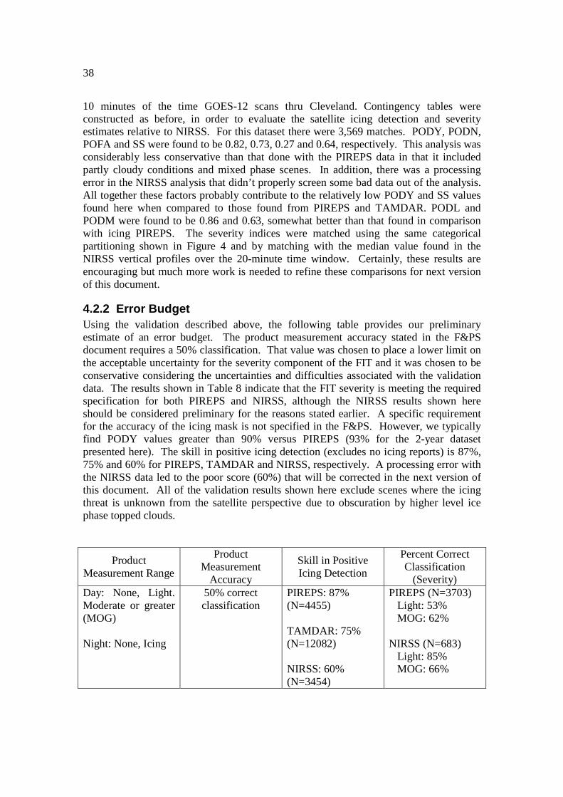
4.2.2 Error Budget.................................................................................................. 38 5 PRACTICAL CONSIDERATIONS ........................................................................... 39

5.1 Numerical Computation Considerations .............................................................. 39

5.2 Programming and Procedural Considerations ..................................................... 39

5.3 Quality Assessment and Diagnostics ................................................................... 39

5.4 Exception Handling ............................................................................................. 39 5.5 Algorithm Validation ........................................................................................... 39

3

6 ASSUMPTIONS AND LIMITATIONS .................................................................... 39

6.1 Performance ......................................................................................................... 39 6.2 Assumed Sensor Performance ............................................................................. 40

6.3 Pre-Planned Product Improvements .................................................................... 40

6.3.1 Estimating the Super-cooled Fraction of Total LWP ................................... 40

6.3.2 Mixed Phase Cloud Effects on the Flight Icing Threat................................. 43

4

LIST OF FIGURES

Figure 1: High level flowchart of the Flight Icing Threat algorithm illustrating the main processing sections............................................................................................................ 15 Figure 2: Ice accreted from super-cooled water droplets on the wing leading edge of a research aircraft while in cloud (Left) and after ascending above cloud (Right). Photo credits: NASA Glenn Research Center. ............................................................................ 17 Figure 3: Cloud phase (Left) derived from GOES-E and GOES-W using the NASA LaRC cloud algorithm and the corresponding icing mask (Right) determined with the ABI FIT algorithm at 1745 UTC on November 8, 2008 .................................................. 19

Figure 4: PIREPS icing intensity for two winter periods (Nov-Mar, 2006/2007 and 2007/2008) over the CONUS and motivation for two-category satellite severity estimate............................................................................................................................................ 20

Figure 5: Relative frequency of icing vs GOES-derived LWP for two winter periods (Nov-Mar, 2006/2007 and 2007/2008) over the CONUS. ............................................... 21

Figure 6: Re-normalized probability of in-cloud aircraft icing as a function of satellite-derived LWP and model fit for two values of Re. ............................................................ 24 Figure 7: The flight icing threat index at 1745 UTC, color coded in McIDAS (Left) and icing severity reported by Pilots (Right) from 16 – 20 UTC on November 8, 2008. ....... 25

Figure 8: SEVIRI RGB image (Left) and results from the ABI cloud phase algorithm (Right) from 12 UTC on November 25, 2005 (courtesy of Michael Pavolonis, NOAA/NESDIS/STAR). .................................................................................................. 27 Figure 9: Cloud liquid water path and effective radius derived from GOES-10 and GOES-12 on November 8, 2008 are critical inputs to the ABI FIT algorithm. These data were derived using the LaRC cloud retrieval algorithm. .................................................. 28 Figure 10: Depiction of the jet routes for the TAMDAR instruments deployed on MESABA Airlines regional jets in early 2005. ................................................................ 30 Figure 11: Example of the icing hazard product produced using NIRSS data at Cleveland’s Hopkins International airport. ....................................................................... 31 Figure 12: Cloud top phase derived from SEVIRI data taken at 1400 UTC on October 19, 2009 using the LaRC algorithm (Left) and the AWG ABI cloud algorithm (Right). 31 Figure 13: Cloud Effective Radius (Re) derived from SEVIRI data taken at 1400 UTC on October 19, 2009 using the LaRC algorithm for liquid clouds (Left) and the AWG ABI cloud algorithm for all clouds (Right). ............................................................................. 32 Figure 14: Cloud water path derived from SEVIRI data taken at 1400 UTC on October 19, 2009 using the LaRC algorithm for liquid clouds (Left) and the AWG ABI cloud algorithm for all clouds (Right). ....................................................................................... 32 Figure 15: The ABI flight icing threat derived from SEVIRI data taken at 1400 UTC on October 19, 2009 using the LaRC cloud products (Left) and the AWG ABI cloud products (Right). ............................................................................................................... 33 Figure 16: Comparison of GOES-derived flight icing threat to TAMDAR icing indicators. Large squares represent the TAMDAR observations while the small squares represent GOES. ............................................................................................................... 37 Figure 17: Mean cloud water content shape factors derived from CloudSat data taken over the CONUS as a function of altitude below cloud top and for different CWP’s and

5

cloud thicknesses. The profiles were derived during the months of November-April in 2007/2008 and 2008/2009 for clouds with top tmperatures between 253K and 273K. ... 41

Figure 18: The flight icing threat at 1745 UTC on November 8, 2008 derived using the current (version 3) ABI FIT algorithm (Left) and a new profiling concept being considered for version shown as a cross-section (Right). ................................................. 42 Figure 19: A McIDAS-V 3-D rendition of icing severity profiles derived from GOES-12 at 1745 UTC on Nov. 8, 2008. .......................................................................................... 43

6

LIST OF TABLES

Table 1: GOES-R flight icing threat product requirements. ............................................. 11

Table 2: ABI channel numbers and wavelengths. The channels used to generate the ABI cloud products used as input to the Flight Icing Threat algorithm are indicated in the right column............................................................................................................................... 12

Table 3: Logic table for mapping the ABI cloud phase and optical depth products to the icing mask. ........................................................................................................................ 18

Table 4(a)-(d): Mean and standard deviation found for satellite-derived cloud parameters matched with Icing PIREPS in three categories: (0 - no icing; 1 – light icing; 2 – moderate or greater icing). Results are shown for the entire matched dataset in (a) and (b) and for the filtered dataset in (c) and (d). .................................................................... 22 Table 5: Table describing the icing probability index output from the ABI FIT algorithm............................................................................................................................................ 24

Table 6: Table describing the icing intensity index output from the ABI FIT algorithm. 25 Table 7: Table describing the FIT index output from the ABI FIT algorithm. ................ 25

Table 8: Two-by-two contingency table used to estimate FIT algorithm skill. ................ 34

Table 9: Frequency of yes/no icing reports found for matched GOES/PIREPS dataset constructed over two winter seasons................................................................................. 35 Table 10: Frequency of two-category icing severity index found for matched GOES/PIREPS dataset constructed over two winter seasons. .......................................... 35

Table 11: Preliminary error budget for the ABI FIT algorithm when applied to the LaRC GDCP using current GOES. ............................................................................................. 39

7

LIST OF ACRONYMS ABI - Advanced Baseline Imager AIT - Algorithm Integration Team ATBD - Algorithm Theoretical Basis Document AWG - Algorithm Working Group CAT – Cloud Algorithm Team CERES Clouds and the Earth’s Radiant Energy System COD – Cloud Optical Depth CONUS – Continental U.S. CPS – Cloud Particle Size CWP – Cloud Water Path DCOMP – Daytime Cloud Optical and Microphysical Properties DPC – Data Processing Center DOE – Department of Energy F&PS - Functional and Performance Specification FAR – False Alarm Ratio FIT – Flight Icing Threat FRAMEWORK – NOAA/NESDIS/STAR GOES-R AIT processing framework GLFE – Great Lakes Fleet Experiment GOES - Geostationary Operational Environmental Satellite GDCP – GOES-Derived Cloud Products GS – Ground System ID - Identification LaRC – Langley Research Center LWC – Liquid Water Content LWP – Liquid Water Path McIDAS – Man-Computer Interactive Data Access System MODIS - Moderate Resolution Imaging Spectroradiometer MOG – Moderate or Greater (icing severity) MSG - Meteosat Second Generation NASA - National Aeronautics and Space Administration NCOMP – Nighttime Cloud Optical and Microphysical Properties NESDIS - National Environmental Satellite, Data, and Information Service NOAA - National Oceanic and Atmospheric Administration NWP - Numerical Weather Prediction PIREPS – Pilot Reports POD – Probability of Detection PODY – Probability of Detection Yes observations PODN – Probability of Detection No observations Re – Effective radius SEVIRI - Spinning Enhanced Visible and Infrared Imager SLW – Super-cooled liquid water STAR - Center for Satellite Applications and Research SZA – Solar Zenith Angler TAMDAR – Tropospheric Airborne Meteorological Data Reporting

8

UW – University of Wisconsin

9

INTRODUCTION

1.1 Purpose of This Document The following algorithm theoretical basis document (ATBD) provides a high level description of and the physical basis for a methodology to infer aircraft flight icing conditions using images taken by the Advanced Baseline Imager (ABI) flown on the GOES-R series of NOAA geostationary meteorological satellites. This document will describe the required inputs, the theoretical foundation of the algorithm, the sources and magnitudes of the errors involved, practical considerations for implementation, and the assumptions and limitations associated with the product and provide a high level description of the physical basis for the detection of the flight icing threat.

1.2 Who Should Use This Document The intended users of this document are those interested in understanding the physical basis of the algorithm and how to use the output of this algorithm to assess the flight icing threat. This document also provides information useful to anyone maintaining or modifying the original algorithm.

1.3 Inside Each Section This document is broken down into the following main sections.

• System Overview: Provides relevant details of the ABI and provides a brief description of the products generated by the algorithm.

• Algorithm Description : Provides all the detailed description of the algorithm

including its physical basis, its input and its output.

• Assumptions and Limitations: Provides an overview of the current limitations of the approach and gives the plan for overcoming these limitations with further algorithm development.

1.4 Related Documents This document relates to other GOES-R ABI product documents:

• GOES-R ABI ATBD for Daytime Cloud Optical and Microphysical Properties (DCOMP)

• GOES-R ABI ATBD for Nighttime Cloud Optical and Microphysical Properties(NCOMP)

• GOES-R ABI ATBD for Cloud Mask • GOES-R ABI ATBD for Cloud Phase • GOES-R ABI ATBD for Cloud Height

10

1.5 Revision History • 12/2008 - Version 0.1 of this document was created by William L. Smith Jr.

Version 1.0 represents the first draft of this document. • 08/2010 - Version 1.0 of this document was created by William L. Smith Jr. In

this revision, version 0.1 was revised to meet 80 % delivery standards. • TBD - Version 2.0 of this document will be created by William L. Smith Jr. In

this revision, version 1.0 will be revised to meet 100 % delivery standards.

2 OBSERVING SYSTEM OVERVIEW This section describes the products generated by the ABI flight icing threat algorithm and the requirements they place on the sensor.

2.1 Products Generated The flight icing threat (FIT) algorithm utilizes ABI derived cloud products to make a determination of the potential existence and location for aircraft icing to the extent it can be detected from satellite observations under certain cloud conditions. The first component of the FIT is an icing mask, to identify which pixels are composed of clouds that pose an icing threat based on the presence of super-cooled liquid water (SLW) at cloud top and the magnitude of the clouds optical depth. The icing mask, determined during the daytime and nighttime, also denotes which pixels contain no icing (‘none’) and pixels where icing is possible but undetectable from the satellite perspective (‘unknown’). In addition, the current icing threat design calls for a 2-category estimate of intensity during the daytime. These categories are denoted as light and moderate or greater (MOG). Thus, during daytime the FIT has an additional component to determine the likelihood of icing and the potential intensity based on the satellite-derived cloud microphysical parameters. During the nighttime, the product output is limited to the icing mask since the ABI infrared channels have little sensitivity to variations in liquid cloud microphysical properties for optically thick clouds and thus, the icing intensity can not be estimated. Thus, the formulation described here provides an icing mask at all times of day and daytime only estimates of the probability of icing occurring in two intensity categories.

2.1.1 Product Requirements The F&PS spatial, temporal, and accuracy requirements for the GOES-R flight icing threat are shown below in Table 1.

11

Nam

e

User &

P

riority

Geographic C

overage (G

, H, C

, M)

Vertical R

es.

Horiz. R

es. M

apping Accuracy

Msm

nt. R

ang M

smnt.

Accuracy

Refresh

Rate/C

overage Tim

e O

ption (Mode 3)

Refresh R

ate Option

(Mode 4)

Data

Latency

Long-

Term

S

tability

Product M

easurement

Precision

Aircraft Icing Threat

GOES-R

FD Cloud Top

2 km

5 km

Day: None, Light, Moderate Or Greater (MOG) Night: None, Possible Icing

50% Correct Classification

60 min

5 min

806 sec

TBD NA

Nam

e

User &

P

riority

Geographic

Coverage

(G, H

, C, M

)

Tem

pral C

overage Q

ualifiers

Product

Extend

Qua

lifiers C

loud Co

ver C

onditions Q

ualifiers

Product

Statistics

Qua

lifier

Aircraft Icing Threat

GOES-R FD Day and night

Quantitative out to at least 60 degrees LZA and qualitative beyond

Clear conditions down to cloud top associated with threshold accuracy

Over specified geographic area

Table 1: GOES-R flight icing threat product requirements.

2.2 Instrument Characteristics The FIT algorithm will be executed for each pixel determined to have a high probability of SLW. Specifically, these are cloudy pixels with cloud top temperatures found by the ABI Cloud Height algorithm to be below freezing and that the ABI Cloud Phase algorithm has determined to be composed of water droplets or mixed phase. Table 2 summarizes the ABI channels that will be used to generate the ABI cloud products needed to run the FIT algorithm. Because the FIT algorithm utilizes cloud products generated by other ABI cloud algorithms, any instrument-related artifacts in those products may be passed along to the FIT. The performance of the algorithm will be sensitive to such issues as sensor or imagery artifacts, instrument noise and imperfections in the knowledge of the sensor response functions to the extent that these affect the ABI cloud products. Calibrated observations are critical because in general, the ABI cloud product algorithms utilize the observed values in conjunction with calculations from a radiative transfer model where accurate radiances are assumed.

12

Channel Number Wavelength (µm) Used in Cloud Product Algorithms

1 0.47 2 0.64 � 3 0.86 4 1.38 5 1.61 6 2.26 � 7 3.9 � 8 6.15 9 7.0 10 7.4 � 11 8.5 � 12 9.7 13 10.35 14 11.2 � 15 12.3 � 16 13.3 �

Table 2: ABI channel numbers and wavelengths. The channels used to generate the ABI cloud products used as input to the Flight Icing Threat algorithm are indicated in the right column.

3 ALGORITHM DESCRIPTION

3.1 Algorithm Overview The FIT algorithm is a straightforward formulation that utilizes a suite of GOES-R ABI cloud products in order to discriminate areas of possible aircraft icing. During the daytime, the probability of encountering icing in one of two intensity categories is also estimated. The formulation is similar to that reported in Minnis et al. (2004a) but the algorithm coefficients and thresholds have been updated using a significantly expanded development dataset. The ABI Cloud Phase and Cloud Optical Depth (COD) products form the basis for the icing mask by indicating the locations of optically thick clouds with tops composed of super-cooled liquid water (SLW). The cloud liquid water path (LWP) is the primary indicator of icing intensity. The cloud particle size (CPS) and LWP are used to estimate the icing probability. The FIT algorithm is classified as an “Option 2” algorithm within the GOES-R GS F&PS document. The algorithm requires the following input to determine the flight icing threat:

• Cloud Phase • Cloud Optical Depth • Liquid Water Path • Cloud Particle Size

13

• Cloud Top Temperature • Cloud Top Height • GFS NWP Model Freezing Level

The FIT algorithm derives the following ABI products listed in the F&PS:

• Icing mask • 2-category icing intensity (daytime only)

In addition, the algorithm determines the following products that are not included in F&PS:

• Icing probability (daytime only) • Top and base altitude of icing layer

3.2 Processing Outline The processing outline of the FIT algorithm is summarized in Figure 1. The current FIT algorithm is implemented within the NOAA/NESDIS/STAR GOES-R AIT framework (FRAMEWORK). FRAMEWORK routines are used to provide all of the necessary ABI derived products and ancillary data.

3.3 Algorithm Input This section describes the inputs needed to process the FIT algorithm. The algorithm is run at the pixel level.

3.3.1 Primary Sensor Data The list below contains the primary sensor data used by the OT and ATC algorithm package. By primary sensor data, we mean information that is derived solely from the ABI observations and geolocation information.

• Solar zenith angle • Sensor viewing zenith angle

3.3.2 Ancillary Data The following data lists and briefly describes the ancillary data required to run the FIT algorithm. By ancillary data, we mean required data that is not directly provided by the ABI observations or geolocation data.

• Numerical Weather Prediction (NWP) Freezing Level The freezing level is needed to provide a lower altitude boundary for the flight icing threat.

14

3.3.3 Derived Data Specific ABI cloud products developed by the cloud algorithm team (CAT) required to run the FIT algorithm include:

• ABI cloud phase output (product developed by cloud team) • ABI cloud optical depth output (product developed by cloud team) • ABI cloud particle size output (product developed by cloud team) • ABI cloud liquid water path output (product developed by cloud team) • ABI cloud top temperature output (product developed by cloud team) • ABI cloud top altitude output (product developed by cloud team)

15

Figure 1: High level flowchart of the Flight Icing Threat algorithm illustrating the main processing sections.

3.4 Theoretical Description Flight icing threat detection from satellite involves the detection of SLW pixels since SLW is a prerequisite for aircraft icing. The FIT algorithm chosen for the GOES-R ABI is a theoretically based method since it utilizes theoretically based cloud parameters derived from satellite radiance data. It is designed to work as a standalone algorithm

16

based solely on passive satellite data. Not all SLW clouds can be detected from passive satellite techniques since they are sometimes obscured by higher cloud layers.

3.4.1 Physics of the Problem It is natural for clouds to contain liquid water droplets at altitudes where the air temperature is below freezing. When SLW comes in contact with a hard surface such as the frame of an aircraft, it freezes, thereby icing the airframe as shown for example in Figure 2. As ice accumulates on an aircraft it alters the airflow, which can increase drag and reduce the ability of the airframe to create lift, leading to control problems with potentially disastrous consequences. A significant percentage of weather-related aviation accidents over the last half-century have been attributed to icing. Typically, the flight icing threat to aircraft is reduced by either protecting the aircraft with de-icing and/or anti-icing equipment or by avoidance, particularly for unprotected aircraft. However, severe icing can overwhelm an aircraft’s icing protection system. Icing conditions can be highly variable, often occurring in small areas that cannot be resolved with current icing diagnosis and forecasting methods, which tend to overestimate the areal coverage of the flight icing threat. Thus, avoidance can be expensive, resulting in significant increases in flight time or delays on the ground. While there have been improvements in systems to mitigate aircraft icing, no phase of aircraft operations is immune to the threat. Icing severity is sensitive to temperature, the cloud liquid water content and the drop size distribution (Rasmussen et al., 1992). Since it is possible to infer these parameters, or closely related parameters, from satellite data (Minnis et al., 1995, 1998, 2004b) and because SLW is often found to accumulate in the top several hundred meters of cloud layers (Rauber and Tokay, 1991), satellite data can be used advantageously to diagnose icing conditions (Ellrod and Nelson, 1995, Smith et al., 2000, 2003, Ellrod and Bailey, 2007). Complicating its definition, however, is the fact that icing also depends on characteristics of the aircraft and other flight parameters such as the type and weight of the aircraft, the duration of exposure to SLW and the accretion rate of ice on the airframe. These aircraft-related factors can not be accounted for explicitly in a satellite-based icing algorithm.

Although it can form anywhere, aircraft icing is most commonly found in two geographical regions over North America (Bernstein et al., 2006). The first includes the Pacific Northwest, western British Columbia, and Alaska. The second is from the Canadian Maritimes and stretching west and southwest to encompass the Great Lakes Region, Ohio River Valley, and Hudson Bay. Much of this area is within the GOES observation domain. Currently, model forecasts and pilot reports (PIREPS) constitute much of the database available to pilots for assessing the icing conditions in a particular area. Such data are often uncertain or sparsely available. The advanced design of GOES-R provides the information needed to quantitatively estimate important properties of clouds, including those that help determine the flight icing threat, such as cloud

17

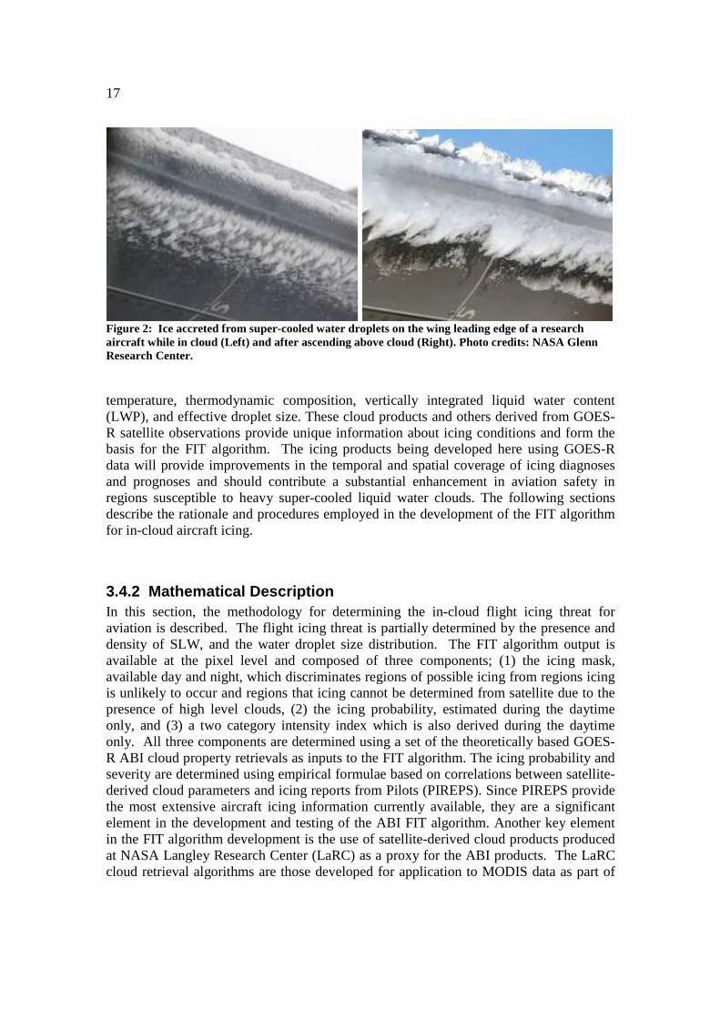
Figure 2: Ice accreted from super-cooled water droplets on the wing leading edge of a research aircraft while in cloud (Left) and after ascending above cloud (Right). Photo credits: NASA Glenn Research Center.

temperature, thermodynamic composition, vertically integrated liquid water content (LWP), and effective droplet size. These cloud products and others derived from GOES-R satellite observations provide unique information about icing conditions and form the basis for the FIT algorithm. The icing products being developed here using GOES-R data will provide improvements in the temporal and spatial coverage of icing diagnoses and prognoses and should contribute a substantial enhancement in aviation safety in regions susceptible to heavy super-cooled liquid water clouds. The following sections describe the rationale and procedures employed in the development of the FIT algorithm for in-cloud aircraft icing.

3.4.2 Mathematical Description In this section, the methodology for determining the in-cloud flight icing threat for aviation is described. The flight icing threat is partially determined by the presence and density of SLW, and the water droplet size distribution. The FIT algorithm output is available at the pixel level and composed of three components; (1) the icing mask, available day and night, which discriminates regions of possible icing from regions icing is unlikely to occur and regions that icing cannot be determined from satellite due to the presence of high level clouds, (2) the icing probability, estimated during the daytime only, and (3) a two category intensity index which is also derived during the daytime only. All three components are determined using a set of the theoretically based GOES-R ABI cloud property retrievals as inputs to the FIT algorithm. The icing probability and severity are determined using empirical formulae based on correlations between satellite-derived cloud parameters and icing reports from Pilots (PIREPS). Since PIREPS provide the most extensive aircraft icing information currently available, they are a significant element in the development and testing of the ABI FIT algorithm. Another key element in the FIT algorithm development is the use of satellite-derived cloud products produced at NASA Langley Research Center (LaRC) as a proxy for the ABI products. The LaRC cloud retrieval algorithms are those developed for application to MODIS data as part of

18

the Clouds and the Earth’s Radiant Energy System (CERES) experiment (Minnis et al., 1995, 1998). The algorithms have been adapted for application to geostationary satellites and are routinely applied to GOES-11 and 12 data, Meteosat SEVIRI, and other satellites, thus providing a significant test-bed for the FIT algorithm.

3.4.2.1 Icing Mask The first step in the FIT algorithm is to construct the icing mask for each geo-located pixel with valid GOES-R radiance data and for which the cloud algorithms have been properly executed and returned valid retrievals. The purpose of the icing mask is to determine which cloudy pixels pose an icing threat to aircraft based on the retrieved cloud properties and to differentiate these pixels from clear and cloudy pixels that pose no icing threat, and from cloudy pixels for which the icing threat cannot be determined (e.g. optically thick pixels composed of high level ice phase clouds). Thus, the output of the icing mask is an index that denotes each valid pixel to be either an icing, no icing, or unknown pixel. The ABI cloud phase product and the cloud optical depth products from DCOMP (for solar zenith angles less than 82°) and NCOMP (for solar zenith angles greater than or equal to 82°) are used to construct the icing mask. The logic is shown in Table 3. In the current version, mixed phase clouds are considered to be an icing threat which is a conservative approach adopted until a better understanding is developed between the mixed phase radiative signals and aircraft icing. This will be explored further when the ABI cloud phase product becomes available over regions where icing validation data are available. For SLW and mixed phase clouds, an optical depth threshold of 1.0 is chosen to eliminate the very thinnest clouds associated with very low LWC values from the icing threat. For ice phase topped clouds, an optical depth threshold of 6.0 is used to eliminate thin clouds from the icing threat that are unlikely to overlap SLW clouds, while the icing threat for thicker clouds, which may or may not overlap SLW clouds, is considered to be unknown. Descriptions of the theoretical basis for determining cloud phase and optical depth can be found in the appropriate ATBD’s developed by the GOES-R ABI CAT. An example of the icing mask is shown in Figure 3

Cloud Phase Cloud Optical Depth Icing Mask Clear NA No Icing Water ALL No Icing

SLW τvis > 1.0 Icing τvis ≤ 1.0 No Icing

Mixed τvis > 1.0 Icing τvis ≤ 1.0 No Icing

ICE τvis ≤ 6.0 No Icing τvis > 6.0 Unknown

Table 3: Logic table for mapping the ABI cloud phase and optical depth products to the icing mask. along with the cloud phase product derived from GOES-E and GOES-W using the NASA LaRC cloud algorithm at 1745 UTC on November 8, 2008. For this case, a large area of clouds over the mid-western states, the Ohio valley and southern Canada, associated with

19

a mid-latitude cyclone, were found to contain SLW in the satellite analysis which contribute to the icing threat as depicted by the cyan colors in the icing mask image. Areas where there is no icing and that the icing threat cannot be determined are denoted by the gray and white colors, respectively. It should be pointed out that a significant

Figure 3: Cloud phase (Left) derived from GOES-E and GOES-W using the NASA LaRC cloud algorithm and the corresponding icing mask (Right) determined with the ABI FIT algorithm at 1745 UTC on November 8, 2008

advance in the accuracy of the icing mask will be realized with the GOES-R ABI due to the additional spectral information and sensitivity to cloud top phase not available on current GOES satellites, particularly at night and during the day/night transition. The fact that the ABI cloud phase algorithm is based on the use of infrared channels only offers consistency in the retrieval of cloud phase and the icing mask for all times of day, unlike methods designed for use with current GOES data which work best during the daytime using solar reflectance channels.

3.4.2.2 Icing Severity The potential for in-cloud aircraft icing and its severity depends on many factors related to the particular aircraft and the weather conditions. Some aircraft will accumulate ice in certain conditions while other aircraft will remain ice-free in the same cloud. These aircraft-related factors are not considered here. Meteorological factors that contribute to icing severity include the concentration of super-cooled water droplets and the droplet sizes. Generally, larger droplets, and/or larger concentrations of droplets or higher liquid water content (LWC) contribute to more severe icing. The satellite-derived effective radius (Re) is sensitive to the cloud droplet sizes and the derived LWP is sensitive to the concentration since it is a measure of the vertically integrated LWC. It may be possible to estimate the LWC profile from the liquid water path (LWP) and the cloud thickness (∆Z) but would require simplifying assumptions. This concept is being explored for a future version of the FIT algorithm and is described below in Section 6.3. The current version of the FIT algorithm has been developed by assuming that LWP serves as a reliable proxy for LWC such that larger values of LWP are associated with larger values of LWC and thus, more severe icing. Development of a two-category severity estimate for the FIT algorithm is based on correlations between satellite-derived cloud parameters and icing PIREPS. The motivation for a two-category scheme is illustrated in figure 4,

20

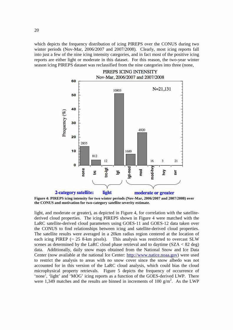
which depicts the frequency distribution of icing PIREPS over the CONUS during two winter periods (Nov-Mar, 2006/2007 and 2007/2008). Clearly, most icing reports fall into just a few of the nine icing intensity categories, and in fact most of the positive icing reports are either light or moderate in this dataset. For this reason, the two-year winter season icing PIREPS dataset was reclassified from the nine categories into three (none,

Figure 4: PIREPS icing intensity for two winter periods (Nov-Mar, 2006/2007 and 2007/2008) over the CONUS and motivation for two-category satellite severity estimate. light, and moderate or greater), as depicted in Figure 4, for correlation with the satellite-derived cloud properties. The icing PIREPS shown in Figure 4 were matched with the LaRC satellite-derived cloud parameters using GOES-11 and GOES-12 data taken over the CONUS to find relationships between icing and satellite-derived cloud properties. The satellite results were averaged in a 20km radius region centered at the location of each icing PIREP (~ 25 8-km pixels). This analysis was restricted to overcast SLW scenes as determined by the LaRC cloud phase retrieval and to daytime (SZA < 82 deg) data. Additionally, daily snow maps obtained from the National Snow and Ice Data Center (now available at the national Ice Center: http://www.natice.noaa.gov) were used to restrict the analysis to areas with no snow cover since the snow albedo was not accounted for in this version of the LaRC cloud analysis, which could bias the cloud microphysical property retrievals. Figure 5 depicts the frequency of occurrence of ‘none’, ‘light’ and ‘MOG’ icing reports as a function of the GOES-derived LWP. There were 1,349 matches and the results are binned in increments of 100 g/m2. As the LWP

21

increases, the number of negative and light icing reports decreases while the number of moderate or greater reports increases. Despite the aforementioned uncertainties associated with icing PIREPS and the fact that they are superimposed on a highly variable cloud field such as the GOES-derived LWP, the results in Figure 5 are encouraging and physically realistic.

Figure 5: Relative frequency of icing vs GOES-derived LWP for two winter periods (Nov-Mar, 2006/2007 and 2007/2008) over the CONUS.

Tables 4a-4d list the results of a statistical analysis performed on the matched satellite and icing PIREPS dataset. The mean and standard deviation for a number of satellite-derived cloud parameters is shown. The values in Table 3(a) and (b) are computed with all the matched data (1,349 points), while the values in Table 3(c) and (d) are computed with a filtered dataset that attempts to reduce some of the ambiguity associated with temporal and spatial errors in the PIREPS data (1,139 points). In the filtering procedure, a set of conservative LWP thresholds are set for specific PIREPS icing intensities based on the assumption that the two are positively correlated as shown in Figure 5. Thus, in the filtered dataset, the matched data are eliminated for the following scenarios: (a) all positive icing reports if LWP < 50 g/m2, (b) all positive icing reports with moderate or greater icing intensity if LWP < 200 g/m2, (c) all icing reports if the intensity is less than light if the LWP > 750 g/m2, and (d) all light icing intensity reports if LWP > 1000 g/m2. Only about 15% (210 points) of the original matched data is eliminated in the filtered dataset. The results in Table 3a ad other analyses (not shown) indicate that there is little dependency found between icing intensity PIREPS and Re. It’s not yet clear weather this is natural behavior or a result of uncertainties in the Re retrievals. The scattering phase function for cloud hydrometeors is extremely sensitive to droplet size when the solar angles and satellite viewing geometry are such that strong

22

backscatter occurs which results in larger uncertainties in the Re retrievals. This phenomenon may occur in the late morning (early afternoon) for GOES-E (GOES-W) over the CONUS in the fall and winter months when icing is most prevalent. More work is needed in this area, using other satellites and multiple-wavelength Re retrievals to better understand the relationship between Re and aircraft icing. A stronger dependence is found for the LWP, but there is not much separation between the mean LWP found for

Table 4(a)-(d): Mean and standard deviation found for satellite-derived cloud parameters matched with Icing PIREPS in three categories: (0 - no icing; 1 – light icing; 2 – moderate or greater icing). Results are shown for the entire matched dataset in (a) and (b) and for the filtered dataset in (c) and (d). the ‘light’ and ‘MOG’ categories when using all of the data. Much stronger sensitivity to LWP is found in the filtered dataset (Table 3c). Also note that the filtered dataset generally produces much lower LWP standard deviations, which implies that the correlation between the icing intensity and the LWP has increased. The weighted average of the mean LWP values shown in Table 3c for the light and MOG categories is found to be 488 g/m2. Based on these results, the current version of the FIT algorithm uses this value as a threshold for icing severity and classifies pixels with LWP > 488 g/m2 as MOG. Icing pixels with LWP ≤ 488 g/m2 are classified as light icing.

23

3.4.2.3 Icing Probability Using the data in Figure 5, the probability of icing was computed and is shown in Figure 6 along with best fit curves for two values of Re intended to represent the upper and lower limits. These relationships were developed by first normalizing the negative icing reports to account for the sampling bias relative to positive icing reports that is apparent in Figure 4. The fact that Pilot’s naturally lack the incentive to report ‘no icing’ is an inherent bias in icing PIREPS that must be accounted for in algorithm development and validation. The probability of icing was then computed and binned as a function of LWP as in Figure 5. Those values were multiplied by the probability of icing found from the data for values of Re = 5 µm (comprised of data with Re < 8 µm) and Re = 16 µm (comprised of data with Re ≥ 16 µm). These two sets of data were then normalized to yield a 100% probability of icing at 1050 g/m2 for Re = 16 µm. The results shown in figure 6 are consistent with our theoretical understanding of icing, indicating an increased likelihood of icing with increased LWP and Re. Based on these results, the icing probability (IP) is formulated in the FIT algorithm as

(1) IP = 0.244ln(LWP) + 0.026, for Re = 5 µm, and

(2) IP = 0.32ln(LWP) + 0.034, for Re = 16 µm. Linear interpolation between the results of (1) and (2) are used for pixels with Re between 5 and 16 µm. Pixels with larger or smaller values of Re are assigned the appropriate extreme value. Values of IP < 0.4 are classified as low probability. For values between 0.4 and 0.7, pixels are classified as medium probability and values exceeding 0.7 are classified as high probability.

24

Figure 6: Re-normalized probability of in-cloud aircraft icing as a function of satellite-derived LWP and model fit for two values of Re.

3.5 Algorithm Output The final output of the flight icing threat (FIT) algorithm includes three sets of indices, which are shown in Tables 5 – 7. The icing probability index and the icing intensity index shown in Tables 5 and 6 are combined into a single FIT index, shown in Table 7, which can be color coded for display purposes. An example of the FIT index output in a McIDAS display is shown in Figure 7 for the same case shown in Figure 3, along with corresponding icing PIREPS near the same time, which confirms the ABI flight icing

Icing Probability Index

Description

-7 No Retrieval/bad data 0 No icing

1 Icing Possible (Nighttime only: SZA ≥ 82°) 2 Low probability of icing (Daytime only: SZA < 82°) 3 Medium probability of icing (Daytime only: SZA < 82°) 4 High probability of icing (Daytime only: SZA < 82°)

Table 5: Table describing the icing probability index output from the ABI FIT algorithm.

Icing Intensity Index

Description

25

-7 No Retrieval/bad data0 No icing1 Unknown2 Light 3 Moderate or greater (MOG) icing (Daytime only: SZA < 82

Table 6: Table describing the icing intensity index output from the ABI FIT algorithm.

FIT Index

-7 No Retrieval/bad data-9 Missing data/other0 No icing1 Unknown2 Low probability of light icing (Daytime only: SZA < 823 Medium probability of light icing (Daytime only: SZA < 824 High probability of light icing (Daytime only: SZA < 825 High probability of MOG 6 Icing Possible (Nighttime only: SZA

Table 7: Table describing the FIT index output from the ABI FIT algorithm. threat. Generally, there is good correspondence between the FIT output and the icing severity PIREPS. It’s apparent how much more information the current FIT product will provide during the daytime compared to a binary yes/no icing product (e.g. Figure 3). The current approach appears to resolve some of the natural variability in the flight icing threat to a significant degree, but of course needs to be validated to the extent possible. This will be discussed further in the validation section below. In additidescribed above, the icing layer boundaries will also be output and are planned to be included in the quality control flags since they are not specifically required in the F&PS requirements.

Figure 7: The flight icing threat index at 1745 UTC, color coded in McIDAS (Left) and icing severity reported by Pilots (Right) from 16

No Retrieval/bad data No icing Unknown Light icing (Daytime only: SZA < 82°) Moderate or greater (MOG) icing (Daytime only: SZA < 82

: Table describing the icing intensity index output from the ABI FIT algorithm.

Description

No Retrieval/bad data Missing data/other No icing Unknown Low probability of light icing (Daytime only: SZA < 82Medium probability of light icing (Daytime only: SZA < 82High probability of light icing (Daytime only: SZA < 82High probability of MOG icing (Daytime only: SZA < 82Icing Possible (Nighttime only: SZA ≥ 82°)

: Table describing the FIT index output from the ABI FIT algorithm.

. Generally, there is good correspondence between the FIT output and the icing severity PIREPS. It’s apparent how much more information the current FIT product will provide during the daytime compared to a binary yes/no icing product (e.g. Figure 3).

current approach appears to resolve some of the natural variability in the flight icing threat to a significant degree, but of course needs to be validated to the extent possible. This will be discussed further in the validation section below. In additidescribed above, the icing layer boundaries will also be output and are planned to be included in the quality control flags since they are not specifically required in the F&PS

ight icing threat index at 1745 UTC, color coded in McIDAS (Left) and icing severity reported by Pilots (Right) from 16 – 20 UTC on November 8, 2008.

Moderate or greater (MOG) icing (Daytime only: SZA < 82°) : Table describing the icing intensity index output from the ABI FIT algorithm.

Low probability of light icing (Daytime only: SZA < 82°) Medium probability of light icing (Daytime only: SZA < 82°) High probability of light icing (Daytime only: SZA < 82°)

icing (Daytime only: SZA < 82°)

. Generally, there is good correspondence between the FIT output and the icing severity PIREPS. It’s apparent how much more information the current FIT product will provide during the daytime compared to a binary yes/no icing product (e.g. Figure 3).

current approach appears to resolve some of the natural variability in the flight icing threat to a significant degree, but of course needs to be validated to the extent possible. This will be discussed further in the validation section below. In addition to the indices described above, the icing layer boundaries will also be output and are planned to be included in the quality control flags since they are not specifically required in the F&PS

ight icing threat index at 1745 UTC, color coded in McIDAS (Left) and icing severity

26

4 TEST DATA SETS AND OUTPUTS

4.1 Simulated/Proxy Input Data Sets The data used to test the ABI FIT algorithm include cloud parameters derived from current GOES, Aqua/Terra MODIS, and SEVIRI. Ideally, the goal is to validate the algorithm using the cloud products produced by the ABI cloud algorithm team. SEVIRI provides the best source of proxy data for the ABI cloud algorithms since the spectral coverage is most similar to that of the ABI. Unfortunately, there are few icing validation data available in the SEVIRI field of view. MODIS is also a good proxy in terms of the spectral coverage but the temporal coverage is limited to just a few times per day. Before this document is finalized, it is expected that a significant effort will be made to test the FIT algorithm on ABI cloud products derived from MODIS over the CONUS but it is uncertain if enough data for icing conditions will be made available to robustly quantify the algorithm performance. To date, most of the quantitative validation of the FIT algorithm has been performed using cloud products derived from current GOES data with the NASA LaRC cloud algorithms over the CONUS where much more icing validation data is available. The results of these efforts are reported here. The LaRC cloud algorithms are also run routinely with SEVIRI data. In the event that a suitable sample of ABI cloud products derived from MODIS, coincident with icing observations, are not made available for quantifying the FIT algorithm uncertainties, we will have to rely on the uncertainty analyses conducted with the LaRC GDCP. In addition, the level of agreement between the LaRC and ABI cloud products will need to be quantified using SEVIRI data. The FIT algorithm will be run using the ABI cloud products from SEVIRI in the Framework and compared to the LaRC results to assure the algorithm is working properly and to test the output for consistency with the LaRC icing product. The FIT algorithm is validated using icing PIREPS, the Tropospheric Airborne Meteorological Data Reporting (TAMDAR) sensor, and data from the NASA Icing Remote Sensing System (NIRSS). These datasets will be described briefly below.

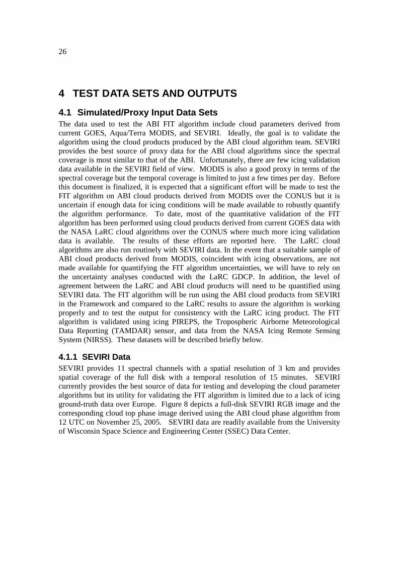
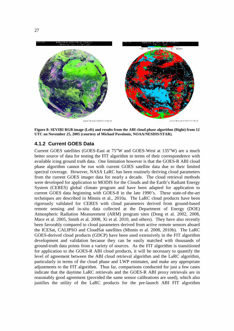
4.1.1 SEVIRI Data SEVIRI provides 11 spectral channels with a spatial resolution of 3 km and provides spatial coverage of the full disk with a temporal resolution of 15 minutes. SEVIRI currently provides the best source of data for testing and developing the cloud parameter algorithms but its utility for validating the FIT algorithm is limited due to a lack of icing ground-truth data over Europe. Figure 8 depicts a full-disk SEVIRI RGB image and the corresponding cloud top phase image derived using the ABI cloud phase algorithm from 12 UTC on November 25, 2005. SEVIRI data are readily available from the University of Wisconsin Space Science and Engineering Center (SSEC) Data Center.

27

Figure 8: SEVIRI RGB image (Left) and results from the ABI cloud phase algorithm (Right) from 12 UTC on November 25, 2005 (courtesy of Michael Pavolonis, NOAA/NESDIS/STAR).

4.1.2 Current GOES Data Current GOES satellites (GOES-East at 75°W and GOES-West at 135°W) are a much better source of data for testing the FIT algorithm in terms of their correspondence with available icing ground truth data. One limitation however is that the GOES-R ABI cloud phase algorithm cannot be run with current GOES satellite data due to their limited spectral coverage. However, NASA LaRC has been routinely deriving cloud parameters from the current GOES imager data for nearly a decade. The cloud retrieval methods were developed for application to MODIS for the Clouds and the Earth’s Radiant Energy System (CERES) global climate program and have been adapted for application to current GOES data beginning with GOES-8 in the late 1990’s. These state-of-the-art techniques are described in Minnis et al., 2010a. The LaRC cloud products have been rigorously validated for CERES with cloud parameters derived from ground-based remote sensing and in-situ data collected at the Department of Energy (DOE) Atmospheric Radiation Measurement (ARM) program sites (Dong et al. 2002, 2008, Mace et al. 2005, Smith et al. 2008, Xi et al. 2010, and others). They have also recently been favorably compared to cloud parameters derived from active remote sensors aboard the ICESat, CALIPSO and CloudSat satellites (Minnis et al. 2008, 2010b). The LaRC GOES-derived cloud products (GDCP) have been used extensively in the FIT algorithm development and validation because they can be easily matched with thousands of ground-truth data points from a variety of sources. As the FIT algorithm is transitioned for application to the GOES-R ABI cloud products, it will be necessary to quantify the level of agreement between the ABI cloud retrieval algorithm and the LaRC algorithm, particularly in terms of the cloud phase and LWP estimates, and make any appropriate adjustments to the FIT algorithm. Thus far, comparisons conducted for just a few cases indicate that the daytime LaRC retrievals and the GOES-R ABI proxy retrievals are in reasonably good agreement (provided the same sensor calibrations are used), which also justifies the utility of the LaRC products for the pre-launch ABI FIT algorithm

28

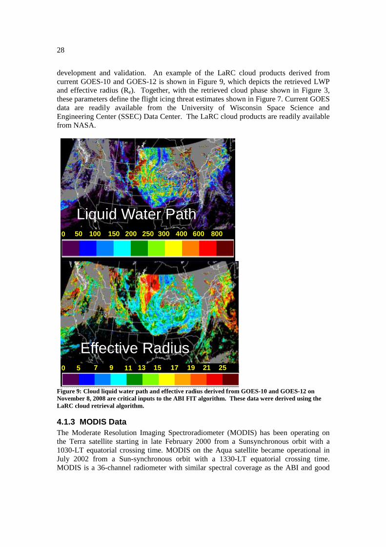
development and validation. An example of the LaRC cloud products derived from current GOES-10 and GOES-12 is shown in Figure 9, which depicts the retrieved LWP and effective radius (Re). Together, with the retrieved cloud phase shown in Figure 3, these parameters define the flight icing threat estimates shown in Figure 7. Current GOES data are readily available from the University of Wisconsin Space Science and Engineering Center (SSEC) Data Center. The LaRC cloud products are readily available from NASA.

Figure 9: Cloud liquid water path and effective radius derived from GOES-10 and GOES-12 on November 8, 2008 are critical inputs to the ABI FIT algorithm. These data were derived using the LaRC cloud retrieval algorithm.

4.1.3 MODIS Data The Moderate Resolution Imaging Spectroradiometer (MODIS) has been operating on the Terra satellite starting in late February 2000 from a Sunsynchronous orbit with a 1030-LT equatorial crossing time. MODIS on the Aqua satellite became operational in July 2002 from a Sun-synchronous orbit with a 1330-LT equatorial crossing time. MODIS is a 36-channel radiometer with similar spectral coverage as the ABI and good

5 7 11 13 17 15 19 21 25 9 0

Effective Radius

0 50 100 150 200 300 250 400 600 800

Liquid Water Path

29

spatial coverage over the CONUS where most of the icing validation data have been collected. Thus, MODIS is a suitable platform to serve as a proxy for testing the FIT algorithm with cloud products derived using the ABI cloud algorithms. This effort is planned for the next version of this document and involves running the ABI cloud algorithm to generate the required cloud product inputs needed for testing the FIT algorithm against the validation data described below. MODIS data are available from the NASA Goddard Space Flight Center Distributed Active Archive Center.

4.1.4 PIREPS Data Pilot reports (PIREPS) constitute the most widely available information on in-flight icing conditions, particularly over the CONUS, but have known deficiencies when used for validation (Kane et al. 1998). They are spatially and temporally biased and the biases are not systematic. PIREPS include severity reports, which should be useful for validating the FIT algorithm severity estimates. However, the severity reports are subjective, based on pilot experience, as well as airframe and flight characteristics, so their accuracy is difficult to characterize. A typical distribution of icing severity PIREPS shown in Fig. 4 for two winter periods over the CONUS indicates that most of the positive reports fall into only two of the eight possible severity categories and there are relatively few negative (‘no icing’) reports. Icing PIREPS have been found to be particularly useful for validating icing detection (Smith et al. 2000) but are inappropriate to compute standard measures of over-warning, such as the False Alarm Ratio (FAR; Brown and Young 2000). Icing PIREPS used in the FIT algorithm development and validation, are easily acquired from the University of Wisconsin Space Science and Engineering Center (SSEC) Data Center.

4.1.5 TAMDAR Data TAMDAR is the Tropospheric Airborne Meteorological Data Reporting sensor currently deployed on approximately 400 commercial aircraft operating over the CONUS, Alaska and Canada. TAMDAR is a low-cost sensor that was developed by AirDat, LLC for NASA. It is designed to measure and report winds, temperature, humidity, turbulence and icing from regional commercial aircraft (Daniels et al., 2002). The TAMDAR icing sensor contains two independent infrared emitter/detector pairs mounted on the probe to detect ice accretion. The accretion of at least 0.5 millimeters of ice on the leading edge surface will block the beams and result in a positive detection. When ice is detected, internal heaters mounted within the probe melt the ice and the measurement cycle repeats. The heaters are powered for at least one minute and the de-icing cycle occurs each time ice is detected. The icing data are given as yes (icing) or no (no icing) reports. Thus, TAMDAR provides a direct, objective measure of in-cloud icing. TAMDAR data are useful for validating icing detection but can not be used reliably to validate the null case or FAR due to difficulties in ascertaining whether the negative icing reports are in cloud or clear air since this is not specifically reported. Attempts to use satellite-derived cloud boundaries matched with the aircraft altitude (which is reported with the icing data) have not sufficiently rectified this problem due to the inaccuracies in the satellite retrievals. TAMDAR data can be acquired from AIRDAT, LLC. Data collected during the Great Lakes Fleet Experiment (GLFE) in 2005 have already been obtained by NASA and are included in the current ABI FIT validation arsenal. Figure 10 shows the Mesaba

30

Airlines regional jet routes for TAMDAR during the GLFE. The current TAMDAR deployment has shifted to the western states and Alaska. These data should also prove useful for validation.

Figure 10: Depiction of the jet routes for the TAMDAR instruments deployed on MESABA Airlines regional jets in early 2005.

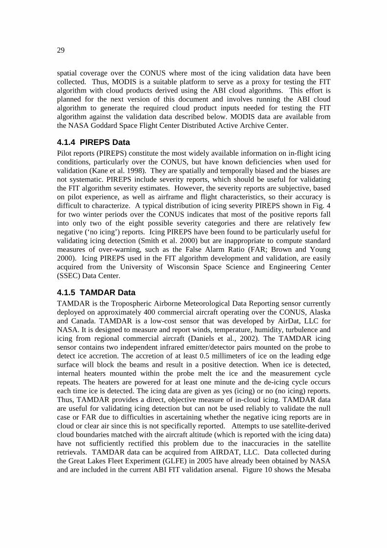
4.1.6 NIRSS Data The NASA Icing Remote Sensing Experiment (NIRSS) has been collecting valuable information on icing conditions that can be used for FIT algorithm testing and validation. The NIRSS has been operating since 2005 at NASA Glenn Research Center in Cleveland, Ohio. This location is well situated for observing icing conditions as it lies in the heart of a climatological icing bulls-eye (Bernstein et al. 2007). The NIRSS was developed to demonstrate a ground-based remote sensing system concept that could provide accurate detection and warning of in-flight icing conditions in the near-airport environment. The system fuses data from radar, lidar, and multi-frequency microwave radiometer sensors to quantify the icing environment and compute the icing hazard (Reehorst et al. 2009) based upon the expected ice accretion severity for the measured environment (Politovitch 2003). Figure 11 shows an example of the icing hazard computed using NIRSS data over a six-hour period. Although the system does not measure icing directly, this remote sensing concept appears to be robust enough to use as a satellite validation tool. For example, it appears that these unique data could also help quantify the FIT algorithm FAR, which cannot be done reliably with any other currently available validation data. Analyses of NIRSS data have just begun for FIT algorithm validation.

Mesaba Airlines Regional Jet Routes

Great Lakes Fleet Experiment (GLFE)

- Dec’04 to May’05

31

Figure 11: Example of the icing hazard product produced using NIRSS data at Cleveland’s Hopkins International airport.

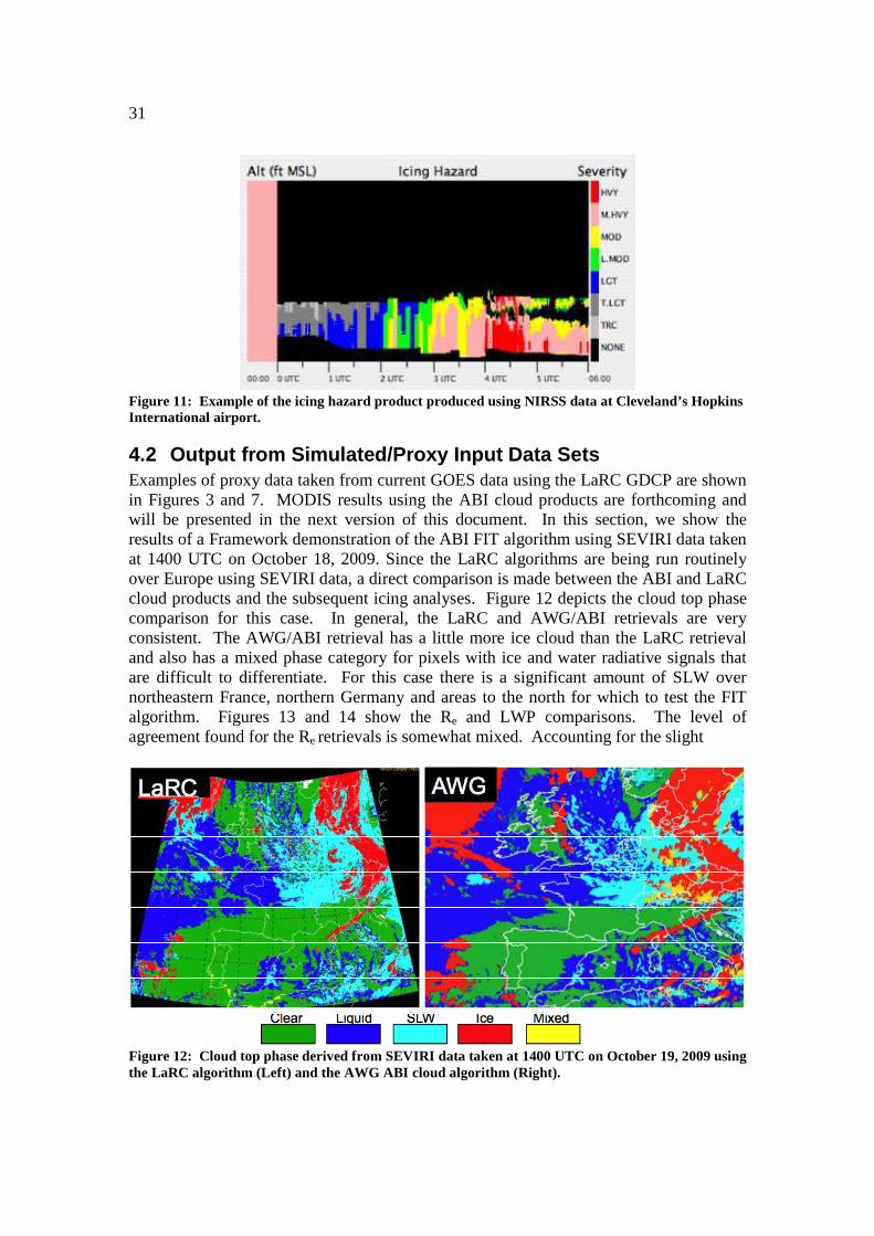
4.2 Output from Simulated/Proxy Input Data Sets Examples of proxy data taken from current GOES data using the LaRC GDCP are shown in Figures 3 and 7. MODIS results using the ABI cloud products are forthcoming and will be presented in the next version of this document. In this section, we show the results of a Framework demonstration of the ABI FIT algorithm using SEVIRI data taken at 1400 UTC on October 18, 2009. Since the LaRC algorithms are being run routinely over Europe using SEVIRI data, a direct comparison is made between the ABI and LaRC cloud products and the subsequent icing analyses. Figure 12 depicts the cloud top phase comparison for this case. In general, the LaRC and AWG/ABI retrievals are very consistent. The AWG/ABI retrieval has a little more ice cloud than the LaRC retrieval and also has a mixed phase category for pixels with ice and water radiative signals that are difficult to differentiate. For this case there is a significant amount of SLW over northeastern France, northern Germany and areas to the north for which to test the FIT algorithm. Figures 13 and 14 show the Re and LWP comparisons. The level of agreement found for the Re retrievals is somewhat mixed. Accounting for the slight

Figure 12: Cloud top phase derived from SEVIRI data taken at 1400 UTC on October 19, 2009 using the LaRC algorithm (Left) and the AWG ABI cloud algorithm (Right).

32

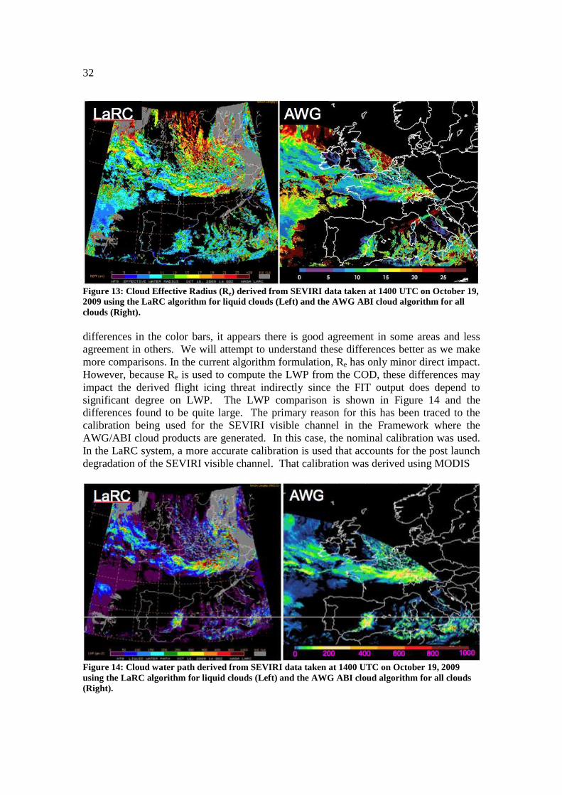
Figure 13: Cloud Effective Radius (Re) derived from SEVIRI data taken at 1400 UTC on October 19, 2009 using the LaRC algorithm for liquid clouds (Left) and the AWG ABI cloud algorithm for all clouds (Right). differences in the color bars, it appears there is good agreement in some areas and less agreement in others. We will attempt to understand these differences better as we make more comparisons. In the current algorithm formulation, Re has only minor direct impact. However, because Re is used to compute the LWP from the COD, these differences may impact the derived flight icing threat indirectly since the FIT output does depend to significant degree on LWP. The LWP comparison is shown in Figure 14 and the differences found to be quite large. The primary reason for this has been traced to the calibration being used for the SEVIRI visible channel in the Framework where the AWG/ABI cloud products are generated. In this case, the nominal calibration was used. In the LaRC system, a more accurate calibration is used that accounts for the post launch degradation of the SEVIRI visible channel. That calibration was derived using MODIS

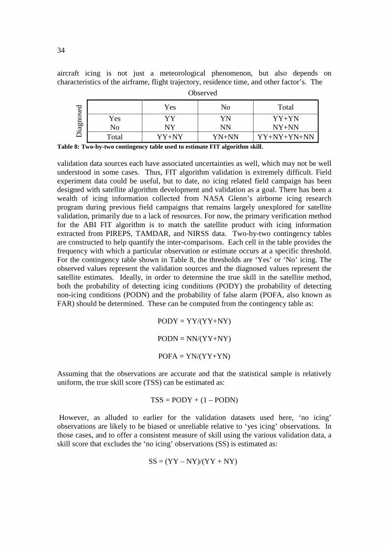
Figure 14: Cloud water path derived from SEVIRI data taken at 1400 UTC on October 19, 2009 using the LaRC algorithm for liquid clouds (Left) and the AWG ABI cloud algorithm for all clouds (Right).

33

data for which the visible channel is well characterized using on-board calibration targets. This explains why the AWG/ABI cloud LWP values are considerably lower than those derived using the LaRC algorithm. Also note that this version of the AWG/ABI cloud algorithm (DCOMP) was not run for SZA > 70°. A future version will run this out to 82° since that is the current plan for operations by the CAT. The flight icing threat derived from the two sets of cloud products is shown in Figure 15. As expected, there are significant differences but this is primarily due to the calibration issue. There were a few icing PIREPS near the same time as this analysis that confirm the satellite-derived flight icing threat. Icing PIREPS are not normally reported over Europe, however these were obtained from Dr. Thomas Hauf at the University of Hannover in Germany as part of a special operations field campaign being conducted by European icing research teams. Despite the differences found between the ABI and LaRC cloud products, this exercise indicates that the ABI FIT algorithm is working as expected in the Framework. The Framework version should yield results that are much more consistent with the LaRC results once the nominal calibration for the visible channel on SEVIRI is replaced with something more accurate, such as the LaRC calibration. In another offline study, COD values from the AWG/ABI algorithm have been compared to the LaRC values for liquid clouds over the eastern Pacific ocean and found to agree quite well. Thus, it appears that the LaRC GDCP could serve as a suitable proxy for characterizing the FIT algorithm uncertainties in lieu of the ABI cloud products should they not be made available with coincident icing observations for testing with MODIS before the GOES-R launch. Clearly, more work is needed to understand the cloud product differences and the possible impacts on the accuracy of the FIT algorithm.

Figure 15: The ABI flight icing threat derived from SEVIRI data taken at 1400 UTC on October 19, 2009 using the LaRC cloud products (Left) and the AWG ABI cloud products (Right).

4.2.1 Precision and Accuracy Estimates To estimate the precision and accuracy of the FIT algorithm, icing information from PIREPS, TAMDAR and NIRSS are used. They each have unique advantages and disadvantages as described briefly in Section 4.1. It’s important to emphasize again that

34

aircraft icing is not just a meteorological phenomenon, but also depends on characteristics of the airframe, flight trajectory, residence time, and other factor’s. The

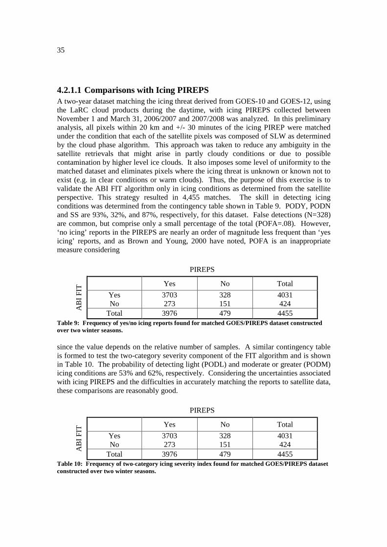
Observed

Dia

gn

osed

Yes No Total

Yes YY YN YY+YN No NY NN NY+NN

Total YY+NY YN+NN YY+NY+YN+NN Table 8: Two-by-two contingency table used to estimate FIT algorithm skill. validation data sources each have associated uncertainties as well, which may not be well understood in some cases. Thus, FIT algorithm validation is extremely difficult. Field experiment data could be useful, but to date, no icing related field campaign has been designed with satellite algorithm development and validation as a goal. There has been a wealth of icing information collected from NASA Glenn’s airborne icing research program during previous field campaigns that remains largely unexplored for satellite validation, primarily due to a lack of resources. For now, the primary verification method for the ABI FIT algorithm is to match the satellite product with icing information extracted from PIREPS, TAMDAR, and NIRSS data. Two-by-two contingency tables are constructed to help quantify the inter-comparisons. Each cell in the table provides the frequency with which a particular observation or estimate occurs at a specific threshold. For the contingency table shown in Table 8, the thresholds are ‘Yes’ or ‘No’ icing. The observed values represent the validation sources and the diagnosed values represent the satellite estimates. Ideally, in order to determine the true skill in the satellite method, both the probability of detecting icing conditions (PODY) the probability of detecting non-icing conditions (PODN) and the probability of false alarm (POFA, also known as FAR) should be determined. These can be computed from the contingency table as:

PODY = YY/(YY+NY)

PODN = NN/(YY+NY)

POFA = YN/(YY+YN) Assuming that the observations are accurate and that the statistical sample is relatively uniform, the true skill score (TSS) can be estimated as:

TSS = PODY + (1 – PODN) However, as alluded to earlier for the validation datasets used here, ‘no icing’ observations are likely to be biased or unreliable relative to ‘yes icing’ observations. In those cases, and to offer a consistent measure of skill using the various validation data, a skill score that excludes the ‘no icing’ observations (SS) is estimated as: SS = (YY – NY)/(YY + NY)

35

4.2.1.1 Comparisons with Icing PIREPS A two-year dataset matching the icing threat derived from GOES-10 and GOES-12, using the LaRC cloud products during the daytime, with icing PIREPS collected between November 1 and March 31, 2006/2007 and 2007/2008 was analyzed. In this preliminary analysis, all pixels within 20 km and +/- 30 minutes of the icing PIREP were matched under the condition that each of the satellite pixels was composed of SLW as determined by the cloud phase algorithm. This approach was taken to reduce any ambiguity in the satellite retrievals that might arise in partly cloudy conditions or due to possible contamination by higher level ice clouds. It also imposes some level of uniformity to the matched dataset and eliminates pixels where the icing threat is unknown or known not to exist (e.g. in clear conditions or warm clouds). Thus, the purpose of this exercise is to validate the ABI FIT algorithm only in icing conditions as determined from the satellite perspective. This strategy resulted in 4,455 matches. The skill in detecting icing conditions was determined from the contingency table shown in Table 9. PODY, PODN and SS are 93%, 32%, and 87%, respectively, for this dataset. False detections (N=328) are common, but comprise only a small percentage of the total (POFA=.08). However, ‘no icing’ reports in the PIREPS are nearly an order of magnitude less frequent than ‘yes icing’ reports, and as Brown and Young, 2000 have noted, POFA is an inappropriate measure considering

PIREPS

AB

I F

IT Yes No Total

Yes 3703 328 4031 No 273 151 424

Total 3976 479 4455 Table 9: Frequency of yes/no icing reports found for matched GOES/PIREPS dataset constructed over two winter seasons. since the value depends on the relative number of samples. A similar contingency table is formed to test the two-category severity component of the FIT algorithm and is shown in Table 10. The probability of detecting light (PODL) and moderate or greater (PODM) icing conditions are 53% and 62%, respectively. Considering the uncertainties associated with icing PIREPS and the difficulties in accurately matching the reports to satellite data, these comparisons are reasonably good.

PIREPS

AB

I FIT

Yes No Total

Yes 3703 328 4031 No 273 151 424

Total 3976 479 4455 Table 10: Frequency of two-category icing severity index found for matched GOES/PIREPS dataset constructed over two winter seasons.

36

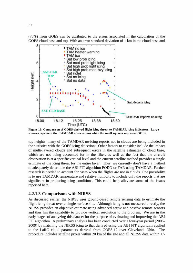
4.2.1.2 Comparisons with TAMDAR Daytime GOES-12 data from April 1-26, 2005 were analyzed with the LaRC cloud algorithm and compared to TAMDAR data taken during the GLFE (Nguyen et al. 2006). The TAMDAR icing data consist of six indices: “I” signifies that icing is occurring and the probe heater is on; “F” indicates an ice-detector fault; “D” means that no icing is indicated; ”H” signifies no icing and the probe heater is on; “L” indicates that icing is occurring and the heater is about to turn on; and “C” means that the heater has shut-off and the probe is cooling down. The post-processed April 2005 data obtained from AirDat contains only the “I”, “D”, and “H” indicators. There were 440,542 observations, of which 13,321 reports indicated icing, 8,951 indicated that the heater was on so icing was not detectable at that time and the rest indicated that no icing was observed. When the TAMDAR probe detects icing, it reports immediately and then at a minimum of every minute thereafter. During aircraft ascent and descent, the probes report more frequently, providing as many as 6 observations per minute to obtain vertical sounding profiles. During level flight, the probes report every 3 minutes. Unlike the few PIREPS reports that are reported (most of which are reported during icing conditions), TAMDAR takes continuous data. Therefore the TAMDAR reports are dominated by 95% no icing indicator. Thus, the GOES and TAMDAR comparison statistics in the results will be biased towards the TAMDAR no-icing category if filters are not properly applied to remove insignificant reports (e.g. from cloud free areas). The pixel-level icing parameters derived from GOES are averaged, by spatially weighting the 4 closest pixels to each TAMDAR observation taken within +/- 15 minutes of the satellite observation. In order to compare the TAMDAR data with GOES without biasing the results, only TAMDAR reports at altitudes within the GOES-derived cloud base and top and in a cloudy condition as defined by GOES were compared. The GOES filters reduced the total number of daytime TAMDAR reports to 32,260 cases. Out of the 32,260 cases, TAMDAR reported 13% icing, 6% heater on, and 81% no ice flags while GOES reported 26% icing, 22% no icing, and 52% unknown (or indeterminate). Figure 16 shows an example of satellite-derived icing indices compared with the TAMDAR icing indicators on a Mesaba flight (with TAMDAR serial number 247) on 22 April 2005 between 18:00-18:30 UTC. This single-layer case shows good agreement between the satellite and TAMDAR. Satellite-derived cloud base and top (small squares) and TAMDAR icing indices (large squares) are plotted as functions of altitude. During the majority of the flight segment, the aircraft was inside the GOES-defined cloud and reported icing which corresponds well with the GOES analysis. During the descent below cloud base, the TAMDAR no longer reported icing while GOES still detected icing. This illustrates the need to properly filter out reports that would bias the TAMDAR and GOES statistics. When TAMDAR detects icing, GOES also detected icing 28% of the time. When TAMDAR indicated no icing, the GOES detected no icing 26% of the time. However, if we exclude the 52% of the GOES ‘unknown’ cases, and consider only cases when TAMDAR detected icing conditions, the probability of a positive detection (PODY) by GOES is 88%. When TAMDAR and GOES both detected no icing, the probability of a null detection (PODN) is 50%. Thus, of the 13% TAMDAR icing detections, GOES missed the icing detection (false negative) in only 4% of these cases. However, the GOES detected icing and TAMDAR detected no icing (false positive) in 75% of the GOES icing cases or 19% of all cases. The high false positive detection

37

(75%) from GOES can be attributed to the errors associated in the calculation of the GOES cloud base and top. With an error standard deviation of 1 km in the cloud base and

Figure 16: Comparison of GOES-derived flight icing threat to TAMDAR icing indicators. Large squares represent the TAMDAR observations while the small squares represent GOES. top heights, many of the TAMDAR no-icing reports not in clouds are being included in the statistics with the GOES icing detections. Other factors to consider include the impact of multi-layered clouds and subsequent errors in the satellite estimates of cloud base, which are not being accounted for in the filter, as well as the fact that the aircraft observation is at a specific vertical level and the current satellite method provides a single estimate of the icing threat for the entire layer. Thus, we currently don’t have a method to adequately determine the ABI FIT algorithm PODN or FAR using TAMDAR. Further research is needed to account for cases when the flights are not in clouds. One possibility is to use TAMDAR temperature and relative humidity to include only the reports that are significant in producing icing conditions. This could help alleviate some of the issues reported here.

4.2.1.3 Comparisons with NIRSS As discussed earlier, the NIRSS uses ground-based remote sensing data to estimate the flight icing threat over a single surface site. Although icing is not measured directly, the NIRSS provides an objective estimate using advanced active and passive remote sensors and thus has the capability to provide vertical resolution to the problem. We are in the early stages of analyzing this dataset for the purpose of evaluating and improving the ABI FIT algorithm. A preliminary analysis has been conducted over a four-year period (2006-2009) by matching the NIRSS icing to that derived using the ABI FIT algorithm applied to the LaRC cloud parameters derived from GOES-12 over Cleveland, Ohio. The procedure includes satellite pixels within 20 km of the site and all NIRSS data within +/-

38

10 minutes of the time GOES-12 scans thru Cleveland. Contingency tables were constructed as before, in order to evaluate the satellite icing detection and severity estimates relative to NIRSS. For this dataset there were 3,569 matches. PODY, PODN, POFA and SS were found to be 0.82, 0.73, 0.27 and 0.64, respectively. This analysis was considerably less conservative than that done with the PIREPS data in that it included partly cloudy conditions and mixed phase scenes. In addition, there was a processing error in the NIRSS analysis that didn’t properly screen some bad data out of the analysis. All together these factors probably contribute to the relatively low PODY and SS values found here when compared to those found from PIREPS and TAMDAR. PODL and PODM were found to be 0.86 and 0.63, somewhat better than that found in comparison with icing PIREPS. The severity indices were matched using the same categorical partitioning shown in Figure 4 and by matching with the median value found in the NIRSS vertical profiles over the 20-minute time window. Certainly, these results are encouraging but much more work is needed to refine these comparisons for next version of this document.

4.2.2 Error Budget Using the validation described above, the following table provides our preliminary estimate of an error budget. The product measurement accuracy stated in the F&PS document requires a 50% classification. That value was chosen to place a lower limit on the acceptable uncertainty for the severity component of the FIT and it was chosen to be conservative considering the uncertainties and difficulties associated with the validation data. The results shown in Table 8 indicate that the FIT severity is meeting the required specification for both PIREPS and NIRSS, although the NIRSS results shown here should be considered preliminary for the reasons stated earlier. A specific requirement for the accuracy of the icing mask is not specified in the F&PS. However, we typically find PODY values greater than 90% versus PIREPS (93% for the 2-year dataset presented here). The skill in positive icing detection (excludes no icing reports) is 87%, 75% and 60% for PIREPS, TAMDAR and NIRSS, respectively. A processing error with the NIRSS data led to the poor score (60%) that will be corrected in the next version of this document. All of the validation results shown here exclude scenes where the icing threat is unknown from the satellite perspective due to obscuration by higher level ice phase topped clouds.

Product Measurement Range

Product Measurement

Accuracy

Skill in Positive Icing Detection

Percent Correct Classification

(Severity) Day: None, Light. Moderate or greater (MOG) Night: None, Icing

50% correct classification

PIREPS: 87% (N=4455) TAMDAR: 75% (N=12082) NIRSS: 60% (N=3454)

PIREPS (N=3703) Light: 53% MOG: 62% NIRSS (N=683) Light: 85% MOG: 66%

39

Table 11: Preliminary error budget for the ABI FIT algorithm when applied to the LaRC GDCP using current GOES.

5 PRACTICAL CONSIDERATIONS

5.1 Numerical Computation Considerations The ABI FIT algorithm is implemented sequentially. Because it relies on the results of other cloud algorithms, the cloud phase, and cloud optical properties from DCOMP and NCOMP, must be run before the FIT algorithm. In addition, an estimate of the freezing level will be required to estimate the lower altitude boundary of the icing threat. That can be obtained from an NWP analysis or forecast.

5.2 Programming and Procedural Considerations The ABI FIT algorithm is run at the pixel level.

5.3 Quality Assessment and Diagnostics The following procedures are recommended for diagnosing the performance of the AI FIT algorithm.

• Maintain database of Icing PIREPS in the GOES-R geographic domain • Apply signal detection theory using PIREPS as truth on a weekly or monthly

basis. • Maintain a close collaboration with the teams developing and validating the cloud

phase and cloud optical properties.

5.4 Exception Handling The FIT algorithm will check the quality and validity of the require cloud parameter inputs before processing. The algorithm also expects the main processing framework to flag any pixels with missing geo-location or viewing geometry information.

5.5 Algorithm Validation See section 4 above.

6 ASSUMPTIONS AND LIMITATIONS The following sections describe the current limitations and assumptions in the current version of the ABI FIT algorithm.

6.1 Performance The following assumptions have been made in developing and estimating the performance of the ABI FIT algorithm. The following list contains the current assumptions (numbered) and proposed mitigation strategies (lettered).

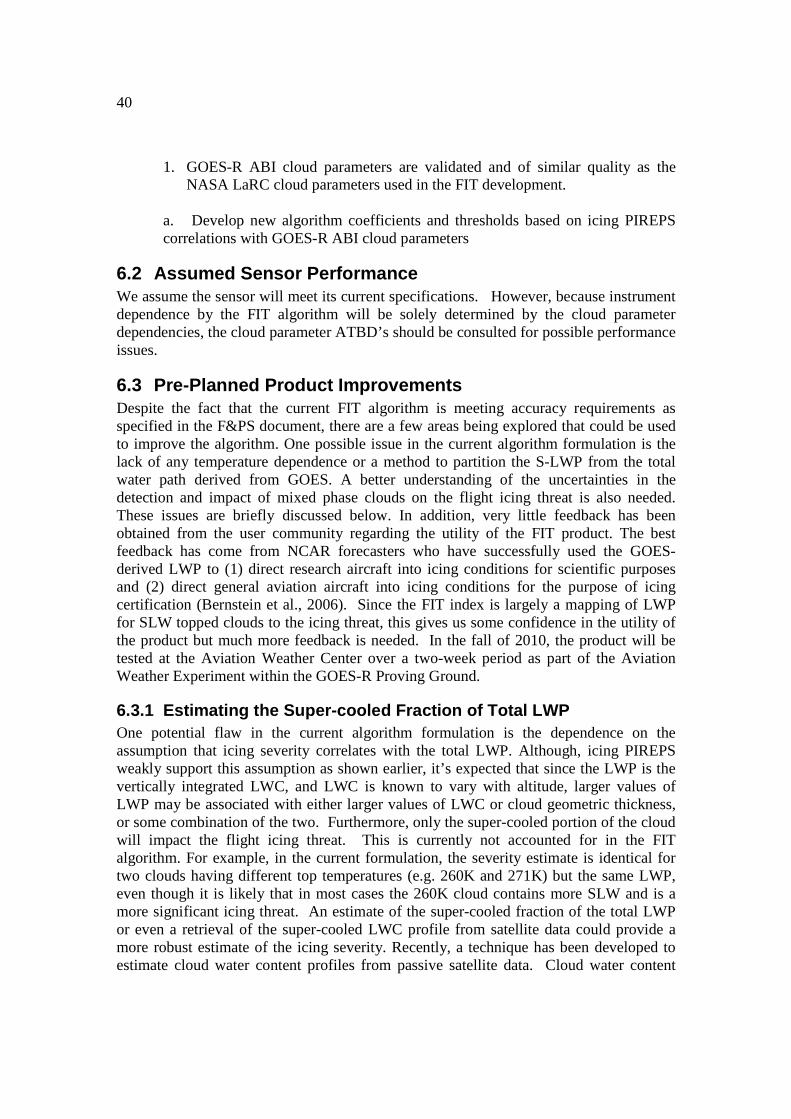
40

1. GOES-R ABI cloud parameters are validated and of similar quality as the

NASA LaRC cloud parameters used in the FIT development. a. Develop new algorithm coefficients and thresholds based on icing PIREPS correlations with GOES-R ABI cloud parameters

6.2 Assumed Sensor Performance We assume the sensor will meet its current specifications. However, because instrument dependence by the FIT algorithm will be solely determined by the cloud parameter dependencies, the cloud parameter ATBD’s should be consulted for possible performance issues.

6.3 Pre-Planned Product Improvements Despite the fact that the current FIT algorithm is meeting accuracy requirements as specified in the F&PS document, there are a few areas being explored that could be used to improve the algorithm. One possible issue in the current algorithm formulation is the lack of any temperature dependence or a method to partition the S-LWP from the total water path derived from GOES. A better understanding of the uncertainties in the detection and impact of mixed phase clouds on the flight icing threat is also needed. These issues are briefly discussed below. In addition, very little feedback has been obtained from the user community regarding the utility of the FIT product. The best feedback has come from NCAR forecasters who have successfully used the GOES-derived LWP to (1) direct research aircraft into icing conditions for scientific purposes and (2) direct general aviation aircraft into icing conditions for the purpose of icing certification (Bernstein et al., 2006). Since the FIT index is largely a mapping of LWP for SLW topped clouds to the icing threat, this gives us some confidence in the utility of the product but much more feedback is needed. In the fall of 2010, the product will be tested at the Aviation Weather Center over a two-week period as part of the Aviation Weather Experiment within the GOES-R Proving Ground.

6.3.1 Estimating the Super-cooled Fraction of Total LWP One potential flaw in the current algorithm formulation is the dependence on the assumption that icing severity correlates with the total LWP. Although, icing PIREPS weakly support this assumption as shown earlier, it’s expected that since the LWP is the vertically integrated LWC, and LWC is known to vary with altitude, larger values of LWP may be associated with either larger values of LWC or cloud geometric thickness, or some combination of the two. Furthermore, only the super-cooled portion of the cloud will impact the flight icing threat. This is currently not accounted for in the FIT algorithm. For example, in the current formulation, the severity estimate is identical for two clouds having different top temperatures (e.g. 260K and 271K) but the same LWP, even though it is likely that in most cases the 260K cloud contains more SLW and is a more significant icing threat. An estimate of the super-cooled fraction of the total LWP or even a retrieval of the super-cooled LWC profile from satellite data could provide a more robust estimate of the icing severity. Recently, a technique has been developed to estimate cloud water content profiles from passive satellite data. Cloud water content

41

profiles for ice and liquid clouds derived from the Cloud Profiling Radar (CPR) on CloudSat are used to develop climatological profiles, or vertical profile shape factors, for different cloud types. The shape factors are then used to distribute the GOES-derived cloud water path in the vertical, which results in a retrieval of the vertical profile of cloud water content. Examples of the shape factors derived from CloudSat for clouds assumed to be composed of SLW between 250K and 273K are shown in Figure 17 as a function of cloud thickness and water path. With knowledge of the freezing level

Figure 17: Mean cloud water content shape factors derived from CloudSat data taken over the CONUS as a function of altitude below cloud top and for different CWP’s and cloud thicknesses. The profiles were derived during the months of November-April in 2007/2008 and 2008/2009 for clouds with top tmperatures between 253K and 273K. obtained from an NWP analysis, these profiles could be used to scale the satellite-derived total water path to estimate the S-LWP. The FIT algorithm could then be reformulated using the S-LWP in the same manner it was originally developed using the total LWP, and re-evaluated to determine if the accuracy has been improved. This is being explored for a future version of the ABI FIT algorithm. Furthermore, this profiling concept for GOES has some similarity to the NIRSS concept with the main exception being that NIRSS uses coincident radar observations to help characterize the vertical distribution of cloud water, whereas this satellite method uses a climatology from CloudSat. Climatologies from other radar and aircraft based observing programs are also being explored for use with this method. NIRSS also has accurate observations of the cloud base from a ceilometer while the passive satellite (i.e. GOES) method utilizes a cloud thickness parameterization to estimate cloud base. Nevertheless, early inter-comparison

∆Z > 3 km ∆Z=1-2 km ∆Z=2-3 km ∆Z=0-1 km

Mean Water Content Shape Factor

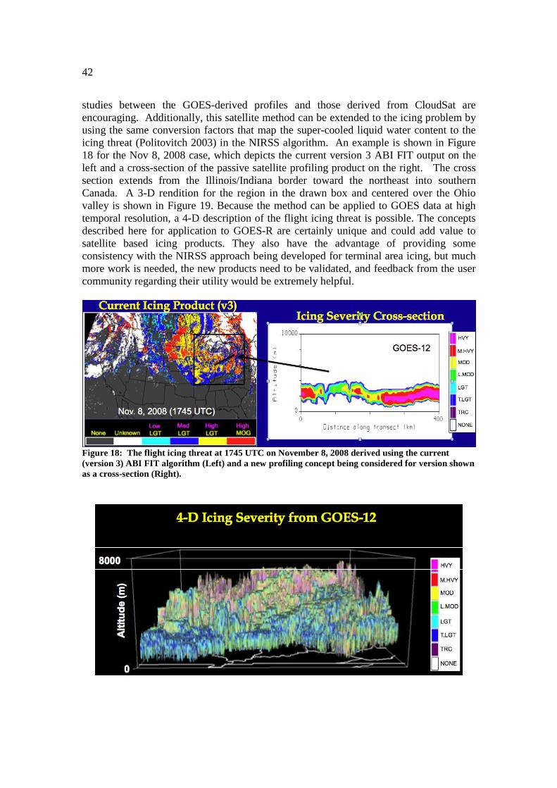
42

studies between the GOES-derived profiles and those derived from CloudSat are encouraging. Additionally, this satellite method can be extended to the icing problem by using the same conversion factors that map the super-cooled liquid water content to the icing threat (Politovitch 2003) in the NIRSS algorithm. An example is shown in Figure 18 for the Nov 8, 2008 case, which depicts the current version 3 ABI FIT output on the left and a cross-section of the passive satellite profiling product on the right. The cross section extends from the Illinois/Indiana border toward the northeast into southern Canada. A 3-D rendition for the region in the drawn box and centered over the Ohio valley is shown in Figure 19. Because the method can be applied to GOES data at high temporal resolution, a 4-D description of the flight icing threat is possible. The concepts described here for application to GOES-R are certainly unique and could add value to satellite based icing products. They also have the advantage of providing some consistency with the NIRSS approach being developed for terminal area icing, but much more work is needed, the new products need to be validated, and feedback from the user community regarding their utility would be extremely helpful.

Figure 18: The flight icing threat at 1745 UTC on November 8, 2008 derived using the current (version 3) ABI FIT algorithm (Left) and a new profiling concept being considered for version shown as a cross-section (Right).

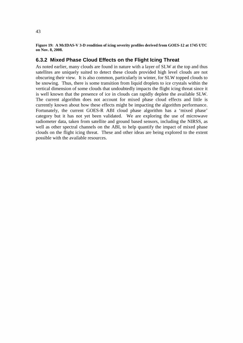
43

Figure 19: A McIDAS-V 3-D rendition of icing severity profiles derived from GOES-12 at 1745 UTC on Nov. 8, 2008.

6.3.2 Mixed Phase Cloud Effects on the Flight Icing Threat As noted earlier, many clouds are found in nature with a layer of SLW at the top and thus satellites are uniquely suited to detect these clouds provided high level clouds are not obscuring their view. It is also common, particularly in winter, for SLW topped clouds to be snowing. Thus, there is some transition from liquid droplets to ice crystals within the vertical dimension of some clouds that undoubtedly impacts the flight icing threat since it is well known that the presence of ice in clouds can rapidly deplete the available SLW. The current algorithm does not account for mixed phase cloud effects and little is currently known about how these effects might be impacting the algorithm performance. Fortunately, the current GOES-R ABI cloud phase algorithm has a ‘mixed phase’ category but it has not yet been validated. We are exploring the use of microwave radiometer data, taken from satellite and ground based sensors, including the NIRSS, as well as other spectral channels on the ABI, to help quantify the impact of mixed phase clouds on the flight icing threat. These and other ideas are being explored to the extent possible with the available resources.

44

REFERENCES

Bernstein, B.C., F. McDonough, C.A. Wolff, M.K. Politovich, G. Cunning, S. Mueller and S. Zednik, 2006: The new CIP icing severity product. Proc. AMS 12th Conf. on Aviation, Range and Aerospace Meteorology, Atlanta GA, 29 Jan - 2 Feb, Amer. Meteor. Soc. Preprint available on CD-rom. Bernstein, B.C., C.A. Wolff and F. McDonough, 2007; An Inferred climatology of icing conditions aloft, including supercooled large drops. Part I: Canada and the Continental United States. J. Appl. Meteor. Clim., 46, 1857-1878. Bernstein, B. C. , C. A. Wolff, and P. Minnis, 2006: Practical application of NASA-Langley advanced satellite products to in-flight icing nowcasts. Proc. 44th AIAA Aerospace Sci. Mtg. & Exhibit, Reno, NV, January 9-12, AIAA-2006-1220, 18 pp. Daniels, T. S., 2002: Tropospheric airborne meteorological data reporting (TAMDAR) sensor development, 2002-02-153, SAE General Aviation Technology Conference and Exposition, Wichita, KS, 16 – 18 April. Dong, X., P. Minnis, G. G. Mace, W. L. Smith, Jr., M. Poellot, R. T. Marchand, and A. D. Rapp, 2002: Comparison of stratus cloud properties deduced from surface, GOES, and aircraft data during the March 2000 ARM Cloud IOP. J. Atmos. Sci., 59, 3256-3284. Dong, X., P. Minnis, B. Xi, S. Sun-Mack, and Y. Chen, 2008: Comparison of CERES-MODIS stratus cloud properties with ground-based measurements at the DOE ARM Southern Great Plains site, J. Geophys. Res., 113, D03204, doi:10.1029/2007JD008438. Ellrod, G. and J. P. Nelson, 1996: Remote Sensing of Aircraft Icing Regions Using GOES Multispectral Imager Data, Proc. AMS 15th Conf. Weather Anal. & Forecasting, 19-23 August, Norfolk, VA, 9-12. Ellrod, G. and A. P. Bailey, 2007: Assessment of Aircraft Icing Potential and Maximum Icing Altitude from Geostationary Meteorological Satellite Data. Wea. Forecasting, 22, 160-174. GOES-R Series Ground Segment (GS) Project Functional and Performance Specification (F&PS) [G417-R-FPS-0089]

GOES-R Acronym and Glossary (P417-R-LIST-0142) Kane, T. L., B.G. Brown, and R. Bruintjes, 1998: Characteristics of pilots reports of icing. Preprints: AMS 14th Conference on Probability and Statistics, 11-16 January, Phoenix, p. 90-95. Mace, G. G., Y. Zhang, S. Platnick, M. D. King, P. Minnis, and P. Yang, 2005: Evaluation of cirrus cloud properties from MODIS radiances using cloud properties

45

derived from ground-based data collected at the ARM SGP site. Journal of Applied Meteorology, 44, 221-240. Minnis, P.; Kratz, D. P.; Coakley, J. A., Jr.; King, M. D.; Garber, D.; Heck, P.; Mayor, S.; Young, D. F. and Arduini, R., 1995: Cloud Optical Property Retrieval (Subsystem 4.3). "Clouds and the Earth's Radiant Energy System (CERES) Algorithm Theoretical Basis Document, Volume III: Cloud Analyses and Radiance Inversions (Subsystem 4)", NASA RP 1376 Vol. 3, edited by CERES Science Team, 135-176. Minnis, P.; Garber, D. P.; Young, D. F.; Arduini, R. F.; and Takano, Y., 1998: Parameterization of reflectance and effective emittance for satellite remote sensing of cloud roperties. Journal of Atmospheric Sciences, 55, 3313-3339. Minnis, P., W. L. Smith, Jr., L. Nguyen, D. A. Spangenberg, P. W. Heck, R. Palikonda, J. K. Ayers, C. Wolff, and J. J. Murray, 2004a: Near-real time cloud properties and aircraft icing indices from GEO and LEO satellites. Proc. SPIE 49th Ann. Mtg., Weather and Environ. Satellites Conf., Denver, CO, August 2-3 5549, 145-155. Minnis, P., L. Nguyen, W. L. Smith, Jr., M. M. Khaiyer, R. Palikonda, D. A. Spangenberg, D. R. Doelling, D. Phan, G. D. Nowicki, P. W. Heck, and C.A. Wolff, 2004b: Real-time cloud, radiation, and aircraft icing parameters from GOES over the USA. Proc. 13th AMS Conf. Satellite Oceanogr. and Meteorol., Norfolk, VA, Sept. 20-24, CD-ROM, P7.1. Minnis, P., C. R. Yost,S. Sun-Mack, and Y. Chen 2008: Estimating the top altitude of optically thick ice clouds from thermal infrared satellite observations using CALIPSO data. Geophys. Res. Lett., L12801, doi:10.1029/2008GL033947. Minnis, P., S. Sun-Mack, D. F. Young, P. W. Heck, D. P. Garber, Y. Chen, D. A. Spangenberg, R. F. Arduini, Q. Z. Trepte, W. L.Smith, Jr., J. K. Ayers, S. C. Gibson, W. F. Miller, V. Chakrapani, Y. Takano, K.-N. Liou, and Y. Xie, 2010a: CERES Edition 2 cloud property retrievals using TRMM VIRS and Terra and Aqua MODIS data: Part I: Algorithms, Submitted to IEEE Trans. Geosci. Remote Sens. Minnis, P., S. Sun-Mack, Y. Chen, M. M. Khaiyer, Y. Yi, J. K. Ayers, R. R. Brown, X. Dong, S. C. Gibson, P. W. Heck, B. Lin, M. L. Nordeen, L. Nguyen, R. Palikonda, W. L. Smith, Jr., D. A. Spangenberg, Q. Z. Trepte, and B. Xi, 2010b: CERES Edition-2 cloud property retrievals using TRMM VIRS and Terra and Aqua MODIS data, Part II: Examples of average results and comparisons with other data. Submitted to IEEE Trans. Geosci. Remote Sens. Nguyen, L., J. J. Murray, P. Minnis, D. P. Garber, J. K. Ayers, D. A. Spangenberg, and M. L. Nordeen, 2006: "Comparison of TAMDAR GLFE icing reports with NASA Advanced Satellite Aviation-weather Products (ASAP) in-flight icing parameters." Proc. AMS 10th Symp. Integr. Observing and Assimil. Systems for Atmos., Oceans, and Land Surf. (IOAS-AOLS), Atlanta, GA, 29 Jan. - 2 Feb., CD-ROM, P9.14.

46

Politovich, M.K., 2003: Predicting inflight aircraft icing intensity. J. Aircraft, 40, 639-644.

Rasmussen, R., and Coauthors, 1992: Winter Icing and Storms Project (WISP). Bull.

Amer. Meteor. Soc., 73, 951-974.

Rauber, R., and A. Tokay, 1991: An explanation for the existence of supercooled water at the top of cold clouds. J. Atmos. Sci., 48, 1005-1023 Reehorst, A., D. Brinker, M. Politovich, D.Serke, C. Ryerson, A. Pazmany, F. Solheim, "Progress Towards the Remote Sensing of Aircraft Icing Hazards". Report NASA/TM-2009-215828,�2009. Smith, W. L., Jr., P. Minnis, and D. F. Young, An icing product derived from operational satellite data. Proc. AMS 9th Conf. Aviation, Range, and Aerospace Meteorol., Orlando, FL, 11-15 Sept., 256-259, 2000. Smith, W. L., Jr., P. Minnis, B. C. Bernstein, A. D. Rapp, and P. W. Heck, 2002: Super-cooled liquid water cloud properties derived from GOES: Comparisons with in situ aircraft measurements. 10th AMS Conf. Aviation, Range, and Aerospace Meteorol., Portland, OR, May 13-16, 89-92. Smith, W. L., Jr., P. Minnis, B. C. Bernstein, F. McDonough, and M. M. Khaiyer, 2003: Comparison of super-cooled liquid water cloud properties derived from satellite and aircraft measurements. Proc. FAA In-Flight Icing/De-icing International Conference, Chicago, IL, June 16-20, CD_ROM, 2003-01-2156. Smith W. L., Jr., P. Minnis, H. Finney, R. Palikonda, and M. M. Khaiyer, 2008: An evaluation of operational GOES derivedsingle-layer cloud top heights with ARSCL over the ARM Southern Great Plains site, Geophys. Res.Lett., vol. 35, L13820, doi:10.1029/2008GL034275. Xi, B., X. Dong, P. Minnis, and M. M. Khaiyer, 2010: A 10-year climatology of cloud cover and vertical distribution derived from both surface and GOES observations over the DOE ARM SGP site. J. Geophys. Res., 115, D12124, doi: 10.1029/2009JD012800.