flight dynamics and simulation of a generic aircraft for ... · este simulador de voo permite...

Flight dynamics and simulation of a generic aircraft foraeroservoelastic design

Pedro Tomás Marques Martins Margarido

Thesis to obtain the Master of Science Degree in

Aerospace Engineering

Supervisor: Prof. André Calado Marta

Examination Committee

Chairperson: Prof. João Manuel Lage de Miranda LemosSupervisor: Prof. André Calado Marta

Member of the Committee: Prof. Agostinho Rui Alves da Fonseca

November 2016

”The dawn mist glowing,

The water flowing,

The endless river,

Forever and ever”

David Gilmour

iii

Acknowledgments

The process of writing a dissertation is exhaustive and arduous - and it is certainly not done single-

handedly.

I want to thank my supervisor, Professor Andre Calado Marta. Thank you Professor, for all your help,

support and specially enthusiasm. I believe that I am tremendously fortunate to have worked with an

outstanding scholar and excellent person.

I would like to thank my parents, Maria and Fernando that helped me become everyday a better

version of myself, and to their sacrifice and dedication over my life, I dedicate them my biggest achieve-

ment, the Master’s. As the oldest brother, I am also deeply thankful to my brothers, Luis and Ines, whose

presence enlightened me and made me more responsible throughout all these years.

I am deeply grateful to my maternal grandparents, Angela and Joao, who cared for me and played

an important role in the development of my identity and shaping the individual that I am today. I was also

extremely fortunate in my life to have paternal grandparents who have shown me unconditional love and

kindness through their life, and I am sorry that they are not present to see me graduate.

I must thank my girlfriend Sara, who gave me strength in the days when I was not in mood of writing

or researching. Through her and her smile I found an easier path for concluding my Master’s, and for

that I am entirely grateful.

Finally, I want to thank all the friends I made throughout this five year journey. Their help and pres-

ence inspired me to reach this goal and without them it would have been certainly been tougher.

v

Resumo

Com o mercado emergente do sector aeronautico, comeca a aparecer a necessidade de ferramentas

que estudem o comportamento aeroservoelastico de uma aeronave. Existem modelos matematicos

para este estudo, porem sao complicados e muitos deles usam o domınio da frequencia.

Nesta dissertacao foram desenvolvidas as equacoes de movimento aeroservoelasticas de uma

aeronave geral para condicoes de equilıbrio no domınio do tempo. Foi desenvolvido um programa pro-

duzido em C++ que integra estas mesmas equacoes, e que no futuro podera ser incluıdo noutros projec-

tos como uma peca de conexao entre diversas areas da aeronautica, como aerodinamica, dinamicas

estruturais e controlo de voo. Para desenvolver esta ferramenta varios metodos de integracao foram

inspecionados e consequentemente encontrando a utilidade de cada um. Consequencias da aeroelas-

ticidade foram tambem discutidas e utilizadas para introduzir o controlo optimo.

Foi tambem realizado um simulador de voo em MATLAB R© utilizando controlo optimo. O compor-

tamento do controlo optimo, mais consequentemente o regulador quadratico linear, nas dinamicas de

voo foi tambem estudado. Este simulador de voo permite simular o movimento de uma aeronave geral,

adoptando um conjunto de derivadas aerodinamicas de aeronaves na literatura, em regimes turbulentos

e em casos de falha de motor em aeronaves com ate cinco motores. O estudo das simulacoes feito

nesta dissertacao teve mais em conta que a aeronave consiga garantir equilıbrio e rumo em situacoes

crıticas, como as acima referidas.

Palavras-chave: dinamica de voo, controlo optimo, aeroservoelasticidade, simulacao de

voo, integracao

vii

Abstract

The emerging market of the aviation sector begins to request the need for tools to study the aeroservoe-

lastic behaviour of an aircraft. There are mathematical models for this kind of study, but its interpretation

is not easy and many use the frequency domain.

In this thesis the aeroservoelastic equations of motion of a general aircraft for equilibrium conditions

in time domain were developed. A program was also developed, produced in C++ R©, which integrates

these same equations, and that in the future may be included in other projects as an interconnection tool

between different fields of aeronautics, such as aerodynamics, structural dynamics and flight control. To

develop this tool, various integration methods were inspected and consequently the utility of each one

was found. Aeroelasticity consequences were also discussed and used to introduce the optimal control.

It was also carried out a flight simulator in MATLAB R© using optimal control. The optimal control

behaviour, more specifically the linear quadratic regulator, in the flight dynamics was also studied. This

flight simulator allows the simulation of the motion for a general aircraft, adopting a set of aerodynamics

derivatives of general aircraft from the literature, on turbulent air flows and in engine failure cases in

aircraft up to five engines. The simulation study in this thesis had more in mind to ensure that the aircraft

maintains its equilibrium and course in critical situations, as referred above.

Keywords: flight dynamics, optimal control, aeroservoelasticity, flight simulation, integration

ix

Contents

Acknowledgments . . . . . . . . . . . . . . . . . . . . . . . . . . . . . . . . . . . . . . . . . . . v

Resumo . . . . . . . . . . . . . . . . . . . . . . . . . . . . . . . . . . . . . . . . . . . . . . . . . vii

Abstract . . . . . . . . . . . . . . . . . . . . . . . . . . . . . . . . . . . . . . . . . . . . . . . . . ix

List of Tables . . . . . . . . . . . . . . . . . . . . . . . . . . . . . . . . . . . . . . . . . . . . . . xv

List of Figures . . . . . . . . . . . . . . . . . . . . . . . . . . . . . . . . . . . . . . . . . . . . . xvii

Nomenclature . . . . . . . . . . . . . . . . . . . . . . . . . . . . . . . . . . . . . . . . . . . . . . xix

Glossary . . . . . . . . . . . . . . . . . . . . . . . . . . . . . . . . . . . . . . . . . . . . . . . . xxv

1 Introduction 1

1.1 Motivation . . . . . . . . . . . . . . . . . . . . . . . . . . . . . . . . . . . . . . . . . . . . . 1

1.2 Topic Overview . . . . . . . . . . . . . . . . . . . . . . . . . . . . . . . . . . . . . . . . . . 2

1.3 Objectives . . . . . . . . . . . . . . . . . . . . . . . . . . . . . . . . . . . . . . . . . . . . . 3

1.4 Thesis Outline . . . . . . . . . . . . . . . . . . . . . . . . . . . . . . . . . . . . . . . . . . 4

2 Theoretical Background 5

2.1 Flight Simulators . . . . . . . . . . . . . . . . . . . . . . . . . . . . . . . . . . . . . . . . . 5

2.1.1 Types of Simulators . . . . . . . . . . . . . . . . . . . . . . . . . . . . . . . . . . . 6

2.1.2 Structure of a Simulator . . . . . . . . . . . . . . . . . . . . . . . . . . . . . . . . . 6

2.2 Aeroelasticity . . . . . . . . . . . . . . . . . . . . . . . . . . . . . . . . . . . . . . . . . . . 7

2.2.1 Static Aeroelasticity . . . . . . . . . . . . . . . . . . . . . . . . . . . . . . . . . . . 7

2.2.2 Dynamic Aeroelasticity . . . . . . . . . . . . . . . . . . . . . . . . . . . . . . . . . . 8

2.3 Aeroservoelasticity . . . . . . . . . . . . . . . . . . . . . . . . . . . . . . . . . . . . . . . . 9

2.3.1 Flutter Control System . . . . . . . . . . . . . . . . . . . . . . . . . . . . . . . . . . 10

2.4 Mathematical Modeling Techniques . . . . . . . . . . . . . . . . . . . . . . . . . . . . . . . 12

2.4.1 P-Transform Technique . . . . . . . . . . . . . . . . . . . . . . . . . . . . . . . . . 12

2.4.2 FAMUSS . . . . . . . . . . . . . . . . . . . . . . . . . . . . . . . . . . . . . . . . . 12

2.4.3 Rational Function Approximation . . . . . . . . . . . . . . . . . . . . . . . . . . . . 13

3 Dynamics Model 15

3.1 Reference Frames and Angles . . . . . . . . . . . . . . . . . . . . . . . . . . . . . . . . . 15

3.1.1 Euler Angles . . . . . . . . . . . . . . . . . . . . . . . . . . . . . . . . . . . . . . . 17

3.1.2 Aerodynamic Angles . . . . . . . . . . . . . . . . . . . . . . . . . . . . . . . . . . . 17

xi

3.1.3 Angular Velocities . . . . . . . . . . . . . . . . . . . . . . . . . . . . . . . . . . . . 18

3.2 Rigid Body Flight Dynamics . . . . . . . . . . . . . . . . . . . . . . . . . . . . . . . . . . . 18

3.2.1 Equations of Motion . . . . . . . . . . . . . . . . . . . . . . . . . . . . . . . . . . . 18

3.2.2 Control Surfaces . . . . . . . . . . . . . . . . . . . . . . . . . . . . . . . . . . . . . 20

3.2.3 Applied Forces and Moments . . . . . . . . . . . . . . . . . . . . . . . . . . . . . . 20

3.2.4 Small Disturbance Theory . . . . . . . . . . . . . . . . . . . . . . . . . . . . . . . . 22

3.2.5 Steady States . . . . . . . . . . . . . . . . . . . . . . . . . . . . . . . . . . . . . . 22

3.2.6 Decoupled Equations . . . . . . . . . . . . . . . . . . . . . . . . . . . . . . . . . . 24

3.2.7 Engine Contribution . . . . . . . . . . . . . . . . . . . . . . . . . . . . . . . . . . . 26

3.3 Elastic Aircraft Consideration . . . . . . . . . . . . . . . . . . . . . . . . . . . . . . . . . . 28

3.3.1 Dynamics of a Flexible Aircraft . . . . . . . . . . . . . . . . . . . . . . . . . . . . . 28

3.3.2 Mathematical Representation of the Dynamics of a Flexible Aircraft . . . . . . . . . 29

4 Flight Dynamics Model Implementation 31

4.1 Flight Dynamics Model Integrator . . . . . . . . . . . . . . . . . . . . . . . . . . . . . . . . 31

4.1.1 Inputs and Outputs . . . . . . . . . . . . . . . . . . . . . . . . . . . . . . . . . . . . 32

4.1.2 Dynamic Equations . . . . . . . . . . . . . . . . . . . . . . . . . . . . . . . . . . . 33

4.1.3 Integration . . . . . . . . . . . . . . . . . . . . . . . . . . . . . . . . . . . . . . . . 33

4.1.4 Type of Steppers . . . . . . . . . . . . . . . . . . . . . . . . . . . . . . . . . . . . . 34

4.2 Stepper Comparison . . . . . . . . . . . . . . . . . . . . . . . . . . . . . . . . . . . . . . . 36

4.3 Aircraft Dynamics . . . . . . . . . . . . . . . . . . . . . . . . . . . . . . . . . . . . . . . . . 37

5 Flight Control and Simulation domain 41

5.1 Simulation Domain . . . . . . . . . . . . . . . . . . . . . . . . . . . . . . . . . . . . . . . . 41

5.2 Sensors and Actuators . . . . . . . . . . . . . . . . . . . . . . . . . . . . . . . . . . . . . . 41

5.3 State-space Systems . . . . . . . . . . . . . . . . . . . . . . . . . . . . . . . . . . . . . . 42

5.3.1 Longitudinal State-space Equations . . . . . . . . . . . . . . . . . . . . . . . . . . 43

5.3.2 Lateral State-space Equations . . . . . . . . . . . . . . . . . . . . . . . . . . . . . 43

5.4 Variable Control . . . . . . . . . . . . . . . . . . . . . . . . . . . . . . . . . . . . . . . . . 43

5.4.1 Coupled Motion . . . . . . . . . . . . . . . . . . . . . . . . . . . . . . . . . . . . . . 44

5.4.2 Longitudinal mode . . . . . . . . . . . . . . . . . . . . . . . . . . . . . . . . . . . . 44

5.4.3 Lateral Mode . . . . . . . . . . . . . . . . . . . . . . . . . . . . . . . . . . . . . . . 45

5.4.4 Heading . . . . . . . . . . . . . . . . . . . . . . . . . . . . . . . . . . . . . . . . . . 46

5.4.5 Flying and Handling Qualities . . . . . . . . . . . . . . . . . . . . . . . . . . . . . . 46

5.5 Atmospheric Perturbations . . . . . . . . . . . . . . . . . . . . . . . . . . . . . . . . . . . 48

5.5.1 Influence on the Model . . . . . . . . . . . . . . . . . . . . . . . . . . . . . . . . . 49

5.5.2 SIMULINK Wind Turbulence Model . . . . . . . . . . . . . . . . . . . . . . . . . . . 50

5.5.3 Disturbances State-space Form . . . . . . . . . . . . . . . . . . . . . . . . . . . . 50

5.6 SIMULINK State-Space model . . . . . . . . . . . . . . . . . . . . . . . . . . . . . . . . . 52

xii

6 Optimal Control and Computational Implementation 53

6.1 Optimal Control Technique - Linear Quadratic Regulator . . . . . . . . . . . . . . . . . . . 53

6.1.1 Aeroservoelastic Optimal Control . . . . . . . . . . . . . . . . . . . . . . . . . . . . 53

6.1.2 Open Loop Aeroservoelastic Problem . . . . . . . . . . . . . . . . . . . . . . . . . 55

6.1.3 Linear Quadratic Regulator . . . . . . . . . . . . . . . . . . . . . . . . . . . . . . . 56

6.1.4 Closed Loop Aeroservoelastic Problem . . . . . . . . . . . . . . . . . . . . . . . . 57

6.1.5 Linear Quadratic Regulator Concerns and Conclusions . . . . . . . . . . . . . . . 59

6.2 Flight Control Coupled Model . . . . . . . . . . . . . . . . . . . . . . . . . . . . . . . . . . 60

6.2.1 Schematic of the Flight Controller Model . . . . . . . . . . . . . . . . . . . . . . . . 60

6.2.2 SIMULINK R© Flight Controller Model . . . . . . . . . . . . . . . . . . . . . . . . . . 62

6.3 Linear Quadratic Regulator Script . . . . . . . . . . . . . . . . . . . . . . . . . . . . . . . . 62

6.3.1 Flying Qualities Evaluator . . . . . . . . . . . . . . . . . . . . . . . . . . . . . . . . 63

6.3.2 Applicable Bryson’s method . . . . . . . . . . . . . . . . . . . . . . . . . . . . . . . 63

7 Flight Simulation 67

7.1 Open-Loop Dynamics . . . . . . . . . . . . . . . . . . . . . . . . . . . . . . . . . . . . . . 67

7.2 Engine Failure . . . . . . . . . . . . . . . . . . . . . . . . . . . . . . . . . . . . . . . . . . 68

7.3 Turbulence . . . . . . . . . . . . . . . . . . . . . . . . . . . . . . . . . . . . . . . . . . . . 72

8 Conclusions 77

8.1 Achievements . . . . . . . . . . . . . . . . . . . . . . . . . . . . . . . . . . . . . . . . . . . 77

8.2 Future Work . . . . . . . . . . . . . . . . . . . . . . . . . . . . . . . . . . . . . . . . . . . . 78

Bibliography 79

A Reference Frames, Stability Derivatives, Flying Qualities and Trim condition Aircraft data 81

A.1 Rotation Matrices . . . . . . . . . . . . . . . . . . . . . . . . . . . . . . . . . . . . . . . . . 81

A.1.1 East North Up Reference Frame . . . . . . . . . . . . . . . . . . . . . . . . . . . . 82

A.2 Stability Derivatives . . . . . . . . . . . . . . . . . . . . . . . . . . . . . . . . . . . . . . . 83

A.3 Flying and Handling Qualities . . . . . . . . . . . . . . . . . . . . . . . . . . . . . . . . . . 83

A.3.1 Aircraft Classes . . . . . . . . . . . . . . . . . . . . . . . . . . . . . . . . . . . . . . 83

A.3.2 Flight Phases . . . . . . . . . . . . . . . . . . . . . . . . . . . . . . . . . . . . . . . 84

A.3.3 Aircraft Data . . . . . . . . . . . . . . . . . . . . . . . . . . . . . . . . . . . . . . . 85

B Aircraft Simulation Data 87

B.1 LQR Q and R Matrices . . . . . . . . . . . . . . . . . . . . . . . . . . . . . . . . . . . . . . 87

B.2 LQR Gain Matrix . . . . . . . . . . . . . . . . . . . . . . . . . . . . . . . . . . . . . . . . . 89

xiii

List of Tables

4.1 Inputs for the flight dynamics integrator scheme . . . . . . . . . . . . . . . . . . . . . . . . 32

4.2 Outputs of the flight dynamics integrator scheme . . . . . . . . . . . . . . . . . . . . . . . 33

4.3 Boost c© and SIMULINK R© types of steppers . . . . . . . . . . . . . . . . . . . . . . . . . . 35

5.1 Aircraft level of perfomance . . . . . . . . . . . . . . . . . . . . . . . . . . . . . . . . . . . 48

7.1 Open-loop dynamic modes eigenvalues for Airbus A400M and Dassault Falcon 7X flight

conditions . . . . . . . . . . . . . . . . . . . . . . . . . . . . . . . . . . . . . . . . . . . . . 67

7.2 A400M - closed loop poles for ε = 10, ε = 40 and ε = 80 . . . . . . . . . . . . . . . . . . . 68

7.3 Falcon 7X - closed loop poles for ε = 2, ε = 20 and ε = 200 . . . . . . . . . . . . . . . . . . 72

A.1 Aircraft classes . . . . . . . . . . . . . . . . . . . . . . . . . . . . . . . . . . . . . . . . . . 83

A.2 Flight phases . . . . . . . . . . . . . . . . . . . . . . . . . . . . . . . . . . . . . . . . . . . 84

A.3 Phugoid flying qualities . . . . . . . . . . . . . . . . . . . . . . . . . . . . . . . . . . . . . 84

A.4 Short period flying qualities . . . . . . . . . . . . . . . . . . . . . . . . . . . . . . . . . . . 84

A.5 Spiral flying qualities . . . . . . . . . . . . . . . . . . . . . . . . . . . . . . . . . . . . . . . 84

A.6 Rolling flying qualities . . . . . . . . . . . . . . . . . . . . . . . . . . . . . . . . . . . . . . 85

A.7 Dutch roll flying qualities . . . . . . . . . . . . . . . . . . . . . . . . . . . . . . . . . . . . . 85

A.8 Aircraft general parameters . . . . . . . . . . . . . . . . . . . . . . . . . . . . . . . . . . . 86

A.9 Aircraft trim derivatives . . . . . . . . . . . . . . . . . . . . . . . . . . . . . . . . . . . . . . 86

xv

List of Figures

1.1 Aeroelasticity . . . . . . . . . . . . . . . . . . . . . . . . . . . . . . . . . . . . . . . . . . . 1

1.2 Aeroservoelasticity model . . . . . . . . . . . . . . . . . . . . . . . . . . . . . . . . . . . . 2

1.3 Dynamics model purpose . . . . . . . . . . . . . . . . . . . . . . . . . . . . . . . . . . . . 3

2.1 VMS NASA simulator . . . . . . . . . . . . . . . . . . . . . . . . . . . . . . . . . . . . . . 5

2.2 Flight simulator structure . . . . . . . . . . . . . . . . . . . . . . . . . . . . . . . . . . . . . 7

2.3 Divergence graphic . . . . . . . . . . . . . . . . . . . . . . . . . . . . . . . . . . . . . . . . 8

2.4 Flutter graphic . . . . . . . . . . . . . . . . . . . . . . . . . . . . . . . . . . . . . . . . . . 8

2.5 Tacoma bridge flutter . . . . . . . . . . . . . . . . . . . . . . . . . . . . . . . . . . . . . . . 8

2.6 Aeroservoelastic interactions . . . . . . . . . . . . . . . . . . . . . . . . . . . . . . . . . . 9

2.7 Aeroservoelasticity block diagram . . . . . . . . . . . . . . . . . . . . . . . . . . . . . . . . 10

2.8 Binary flutter system with a control surface . . . . . . . . . . . . . . . . . . . . . . . . . . 11

3.1 Fixed and relative reference frame . . . . . . . . . . . . . . . . . . . . . . . . . . . . . . . 15

3.2 Euler reference frame rotation . . . . . . . . . . . . . . . . . . . . . . . . . . . . . . . . . . 17

3.3 Control surfaces deflection conventions . . . . . . . . . . . . . . . . . . . . . . . . . . . . 20

3.4 Applied forces on a general aircraft . . . . . . . . . . . . . . . . . . . . . . . . . . . . . . . 20

4.1 Dynamic response of Dassault Falcon 7X flight condition . . . . . . . . . . . . . . . . . . . 36

4.2 Embraer E120 dual flight condition trajectory in the ENU reference frame . . . . . . . . . 38

4.3 Embraer E120 dual flight condition trajectory, XY and YZ planes in the ENU reference frame 38

4.4 Dynamic response of Embraer E120 . . . . . . . . . . . . . . . . . . . . . . . . . . . . . . 40

5.1 Control surfaces actuators model implemented in SIMULINK R© . . . . . . . . . . . . . . . 42

5.2 SIMULINK wind turbulence model . . . . . . . . . . . . . . . . . . . . . . . . . . . . . . . 50

5.3 State-Space in SIMULINK . . . . . . . . . . . . . . . . . . . . . . . . . . . . . . . . . . . . 52

6.1 Airfoil model used in the aeroservoelastic simulation . . . . . . . . . . . . . . . . . . . . . 54

6.2 Below flutter velocity V = 289.6 m/s on open-loop . . . . . . . . . . . . . . . . . . . . . . . 55

6.3 Flutter velocity V = Vflutter = 297.4 m/s on open-loop . . . . . . . . . . . . . . . . . . . . 55

6.4 Over flutter velocity V = 304.8 m/s on open-loop . . . . . . . . . . . . . . . . . . . . . . . 56

6.5 Flutter velocity V = Vflutter = 297.4 m/s on closed-loop with LQR . . . . . . . . . . . . . . 58

6.6 Over flutter velocity V = 304.8 m/s on closed-loop with LQR . . . . . . . . . . . . . . . . . 58

xvii

6.7 Schematic of the control law . . . . . . . . . . . . . . . . . . . . . . . . . . . . . . . . . . . 61

6.8 Flight controller model in SIMULINK . . . . . . . . . . . . . . . . . . . . . . . . . . . . . . 62

6.9 Schematic used for applying Bryson’s method . . . . . . . . . . . . . . . . . . . . . . . . . 64

7.1 A400M’s dynamic responses of the control input variables (δE ,δA,δR) for three different

control penalty parameters (ε = 10, ε = 40 and ε = 80) . . . . . . . . . . . . . . . . . . . . 69

7.2 A400M’s dynamic responses of the non-malfunctioning engines (δT3,δT4

) for three different

control penalty parameters (ε = 10, ε = 40 and ε = 80) . . . . . . . . . . . . . . . . . . . . 70

7.3 A400M’s dynamic responses of the controllable states (u,γ,λ) for three different control

penalty parameters (ε = 10, ε = 40 and ε = 80) . . . . . . . . . . . . . . . . . . . . . . . . . 71

7.4 A400M’s flight trajectory seen in XYENU and Y ZENU planes for three different control


7.5 Falcon 7X’s dynamic responses of the controllable states (u,γ,λ) for three different control


7.6 Falcon 7X’s dynamic responses of the input variables (δE ,δA,δR) for three different control


7.7 Falcon 7X’s dynamic responses of the engines (δT1,δT2

,δT3) for three different control


7.8 Falcon 7X’s Turbulent flight trajectory seen in XYENU and Y ZENU planes for three differ-

ent control penalty parameters (ε = 2, ε = 20 and ε = 200) . . . . . . . . . . . . . . . . . . 75

A.1 Rotation matrix axis system . . . . . . . . . . . . . . . . . . . . . . . . . . . . . . . . . . . 81

xviii

Nomenclature

Greek symbols

α Angle of attack

β Angle of side-slip

χi Velocity of the asymmetrical ith vibration mode

∆t Time interval

δA Aileron deflection

δE Elevator deflection

δR Rudder deflection

δTi Engine throttle relative to the ith engine

ε Control penalty parameter

ηij Structural derivative of the ith symmetrical vibration mode in respect to j

γ Flight path angle

κ Eigenvalue

λ Heading angle

λi Displacement of symmetrical ith vibration mode

Ω Angular speed of the fixed reference frame relatively to the body reference frame

µij Structural derivative of the ith asymmetrical vibration mode in respect to j

ν Plunge angle

ω Natural frequency

ωn Undamped natural frequency

φ Roll angle

π Pi constant

xix

ψ Yaw angle

ρ Density

σi Velocity of the symmetrical ith vibration mode

τi Displacement of asymmetrical ith vibration mode

θ Pitch angle

ξ Damping ratio

Roman symbols

Mi i indirectly induced moment derivative on the y-axis

aij Acceleration on the i-axis in the j reference frame

cg Center of gravity

CDi Drag coefficient derivative with respect to i

cji Coefficient j (j = 1, j = 2 and j = 3) of the ith generalized coordinate

CLi Lift coefficient derivative with respect to i

Cli Rolling moment coefficient derivative with respect to i

Cmi Pitching moment coefficient derivative with respect to i

Cni Yawing moment coefficient derivative with respect to i

CYi Side slip moment coefficient derivative with respect to i

FB Body reference frame

FE Fixed reference frame

Fai Aerodynamic forces on the reference frame i

Fgi Weight force on the reference frame i

Fpi Propulsive forces on the reference frame i

Iθ Wing section static moment about elastic axis

Iij Moment of inertia on the ij axis

Kδ Linear spring constant for torsion stiffness

Kν Linear spring constant for wing bending

L′i i asymmetrical induced moment derivative on the x-axis

Lδ Control induced lift

xx

Lθ Induced aerodynamic lift forces

Li i symmetrical induced moment derivative on the x-axis

Lij Rotation matrix from reference frame j to reference frame i

Mδ Control induced moment

Mθ Motion-induced moment

Mi i directly induced moment derivative on the y-axis

N ′i i asymmetrical induced moment derivative on the z-axis

Ni i symmetrical induced moment derivative on the z-axis

Neng Number of engines

Nsteps Number of integration steps

pdF Flutter dynamic pressure

qi Generalized coordinate

Sθ Wing static moment

u Longitudinal velocity

ui Longitudinal velocity in the reference frame i

v Lateral velocity

vi Lateral velocity in the reference frame i

VFlutter Flutter Velocity

w Vertical velocity

wi Vertical velocity in the reference frame i

Xi i induced force derivative on the x-axis

xi x position in the reference frame i

Yi i induced force derivative on the y-axis

yi y position in the reference frame i

Zi i induced force derivative on the z-axis

zi z position in the reference frame i

Ai Aerodynamic force matrix coefficient with respect to i

ALat Lateral state coefficient matrix

xxi

ALongλs Lateral state coefficient matrix including λ and integrator states

ALong Longitudinal state coefficient matrix

ALQR LQR state coefficient matrix

ALongγ Longitudinal state coefficient matrix including γ state

ALongλ Lateral state coefficient matrix including λ state

ALonguγs Longitudinal state coefficient matrix including γ and integrator states

Bcoupled Engine coupled driving matrix with the updated states

Bini Initial engine coupled driving matrix

BLat Lateral driving matrix

BLongλs Lateral driving matrix including λ and integrator states

BLong Longitudinal driving matrix

BLQR LQR driving matrix

BLongγ Longitudinal driving matrix including γ state

BLongλ Lateral driving matrix including λ state

BLonguγs Longitudinal driving matrix including γ and integrator states

B Damping matrix

dcoupled Disturbance states vector

ei Unit vector in the reference frame i

Ecoupled Associated disturbance influence matrix

F Generalized force; resultant of all external forces

H Total moment

I Inertia tensor matrix; identity matrix

Ks Stiffness matrix

Ki Gain matrix associated with the ith variable

KLQR Gain matrix associated with the LQR method

M Mass matrix; resultant external moment

pi Position vector in the reference frame i

Q State weighting matrix

xxii

q Motion vector

R Control cost matrix

ucoupled Longitudinal and Lateral coupled input vector

uLat Lateral input vector

uLong Longitudinal input vector

v True airspeed

w Angular velocity vector

xLat Lateral state vector

xLongλs Lateral state vector including λ and integrator states

xLong Longitudinal state vector

xLQR LQR state vector

xLongγ Longitudinal state vector including γ state

xLongλ Lateral state vector including λ state

xLonguγs Longitudinal state vector including γ and integrator states

x Generalized deflection; state vector

A Generalized aerodynamic influence coefficient

b Wing span

c Cord

g Gravitational constant

h Height

L Total moment on the x-axis

M Total moment on the x-axis

M Wing section mass

m Mass

N Total moment on the x-axis

p Roll rate

q Pitch rate

r Yaw rate

xxiii

S Wing area

V Flight velocity

X Total force on the X-axis

Y Total force on the x-axis

Z Total force on the x-axis

Subscripts

x, y, z Cartesian components.

0 Equilibrium state

a Aerodynamic force

B Body reference frame

dr Dutch roll dynamic mode

E Fixed reference frame

g Gust

i Dummy index

max Maximum

p Propulsive force

phu Phugoid dynamic mode

ref Reference

roll Roll dynamic mode

sp Short period dynamic mode

spi Spiral dynamic mode

W Wind

Superscripts

* Augmented

T Transpose

xxiv

Glossary

AFC Automatic Flight Controller

AIC Aerodynamic influence coefficient

ASE Aeroservoelasticity

CM Center of mass

DCM Direct cosine matrix

ECEF Earth-Centered Earth-Fixed

ENU East-North-Up

EOM Equations of motion

FAMUSS Flexible Aircraft Modeling Using State Space

FCS Flight Control System

LLH Latitude-Longitude-Height

LQR Linear Quadratic Regulator

NED North-East-Down

ODE Ordinary differential equations

RFA Rational Function Approximation

RPM Rotor rotation speed

RPY Roll-Pitch-Yaw

STL Standard Template Library

TAS True airspeed

xxv

Chapter 1

Introduction

1.1 Motivation

With the increasing growth of high-performance and cheap aircraft, the need for more realistic flight

simulators also grows. One of the crucial aspects on making the flight simulator more realistic is the

consideration of aircraft’s elastic properties (aeroelasticity).

Aeroelasticity has been defined as a science which studies mutual interactions between aerodynamic

forces and elastic forces, and the influence of these interactions on airplane design. Some of the most

rough phenomena on aircraft’s structure happen because of the aircraft’s elastic properties. These

physical phenomena, as they will be described later, can be, for example, flutter, control reversal and

others.[1].

Figure 1.1: Aeroelasticity (adapted from [2])

Traditionally, aeroelasticians utilize frequency domain to model the aeroelastic aircraft, which brings

several concerns since the modern control theory is based primarily on the state-space approach, in

which it requires the aircraft to be modeled in the time domain. The coordinate system on which each

1

scientific area works on, also changes. The flight control engineer usually works in a body axis coordi-

nate system while the aeroelastician works in a mean axis system [3].

This dissertation is about reaching a consensus around these two problems by formulating a mathe-

matical numerical model and then implementing a flight dynamics integrator of the equations of motion,

for a future use in an aeroservoelastic model of a generic aircraft. A flight controller with the possibility

of being embedded in the aeroservoelastic model in the future, was also developed.

1.2 Topic Overview

The focus of this dissertation is firstly the formulation of the equations of motion of a generic elastic

aircraft, in which several areas like Flight dynamics, Aerodynamics, Aeroelasticity will be reviewed. Af-

terwards in order to implement the control laws on the model, Optimal Control laws will also be studied

concerning the implemented law, LQR (Linear Quadratic Regulator). On the basis of this model an au-

tomatic pilot was created, with the possibility of controlling the longitudinal velocity, the flight path angle

and the heading angle.

Figure 1.2: Aeroservoelasticity Model (altered from [4])

The goal is developing an aeroservoelastic model, like in Figure 1.2, for a generic aircraft. Initially

the model, in order to start the simulation, will use a certain aircraft’s aerodynamic and structural model

to form a modal database. The integrated cycle of the model will take in consideration several effects,

like the ones seen in the Figure 1.2, applying a minor update in the aeroservoelastic model. In this

project, only control and gust effects will be taken in consideration since the intention of this dissertation

is to reach the elastic aircraft decoupled equations and create a flight controller and a flight dynamics

integrator. All the simulation of the real-time aeroelastic effects, to be integrated to the flight controller,

could be a possible dissertation work for future students.

2

1.3 Objectives

The main objective of this thesis is the mathematical formulation and respective numerical implemen-

tation of the longitudinal and lateral equations of motion (EOM) of an aircraft, to be embedded in a

aeroservoelasticity analysis and to become an optimization tool in the future. To this end, principles of

flight dynamics, flight control and aeroelasticity will be used to model the system.

Once the system is defined, it should allow the modeling of the aircraft motion in time domain for sim-

ulation purposes. The flight simulator will be done in a MATLAB R© environment and the flight dynamics

integrator will be written in C/C++ R© for computational resource optimization and to facilitate integration

with other tools.

For the flight simulation tool, the control of flight path angle, the heading angle and the longitudinal

velocity, will be applied utilizing the LQR optimal control technique. This flight simulation tool will be of a

generic aircraft, adopting a set of aerodynamics derivatives of aircraft of interest from the literature.

As seen in Figure 1.3, the goal of the flight dynamics integration tool is to guarantee future integration

with aerodynamics, structures, flight control and engine model programs to simulate a generic aircraft

dynamics during a time interval (∆t). The grey highlighted boxes are the programs done and described

throughout this thesis.

Figure 1.3: Purpose behind the flight dynamics integrator

To create these modules, several steps were carried out, namely:

• formulation mathematical of the equations of motion for an elastic aircraft;

• implementation of the flight dynamics model on C/C++;

• interpretation of the several possible integration types;

• implementation of control laws on the mathematical model;

• implementation of the numerical model on MATLAB R© and SIMULINK;

• flight simulation of a generic aircraft on several environments;

3

1.4 Thesis Outline

This thesis is structured in eight Chapters.

The first Chapter introduces the study that will be developed and it has the purpose of contextualizing.

Beyond that, objectives are announced.

The second Chapter contains theoretical background and in it, flight simulators structure and its

different types and functionalities are presented. Then the following concepts of aeroelasticity, including

its two types and different phenomena, and aeroservoelasticity, the capacity of using control inputs to

prevent this phenomena, are introduced. Finally to end the Chapter, different types of mathematical

modelling techniques for aeroservoelastic models are discussed.

The flight dynamics model used is demonstrated on the third Chapter. Firstly, the reference frames

are described and explained, alongside with the Euler angles, aerodynamic angles and angular veloci-

ties. Secondly, rigid body equations of motion are deduced, and by utilizing the small disturbance theory,

two set of equations characterizing the aircraft motion emerge. Single engine contribution is specified for

these equations, generating a set of equations coupled by engine thrust. To conclude the Chapter, the

final trim condition aeroservoelastic set of equations are defined by adding structural bending modes.

The fourth Chapter contains the flight dynamics model implementation, starting by the description of

the process that formulates a C++ integrator program that is capable of integrating the final equations of

Chapter three. The type of integration, what integration stepper to use, outputs and inputs are discussed

throughout this Chapter.

The fifth one is relative to flight control and the simulation domain utilized. The state-space form is

introduced as the domain used for the flight controller. So, the set of equations of motion of Chapter three

is now defined into state-space form. Then, the desired controllable states are introduced into the state-

spaces. Actuators and sensors of the flight controller are discussed here. Flying and handling qualities,

as an important concept of defining realistic flight simulations, are here announced. The atmospheric

perturbations influence on the model is brought in by the end of the Chapter.

The sixth Chapter refers to optimal control and computational implementation of the problem in ques-

tion. The optimal control technique - linear quadratic regulator - is here explained by adopting a classic

aeroelastic foil. Then, it is adopted to this thesis flight controller by being applied to a general aircraft

using the Bryson’s method. In the end of this Chapter, the final flight simulator SIMULINK model and the

script that is used to guarantee level one flight qualities are shown and deliberated upon.

The seventh Chapter yields the flight simulation results. This Chapter is devoted to discussing the

results of two simulations in two different scenarios, engine failure and turbulent flight, for two completely

different aircraft, Airbus A400M and Dassault Falcon 7X. The linear quadratic regulator influence on

these simulations is the prime discussion factor of this Chapter.

The eighth Chapter is where the final conclusions are drawn and future work to be implemented is

defined.

4

Chapter 2

Theoretical Background

In this Chapter, several topics will be studied, such as: Flight simulation, in order to know how this

dissertation project can be embedded in a flight simulator; Aeroelasticity to learn the aeroelastic effects

that need to be prevented; Aeroservoelasticity to control those aeroelastic phenomena; Mathematical

and numerical methods to simulate unsteady aerodynamics and structural dynamics.

2.1 Flight Simulators

Flight simulation is basically a way to recreate the conditions of a real flight. Several aeronautical areas

such as flight dynamics, navigation and aeroelasticity behavior can be studied in an artificial computa-

tional environment.

Figure 2.1: VMS, simulator build by NASA in Ames, California USA

From actually large built simulators, as seen in Figure 2.1, to flight simulator games, flight simulation

has found its use for both professional and casual purposes. One of the most useful traits of flight

simulation is to enable military or civil pilots to train. Being in a simulated environment allows the training

of life-treating maneuvers, practicing of complex missions and, of course, the enhancement piloting skills

[5]. The benefits of flight simulation are:

1. Safety: As said before, flight simulation allows pilots to face dangerous situations that may happen

5

in a real flight. It also allows inexperienced pilots to gather motor skills and the basic procedures

of flight. Simulators are also used as testing devices for new designed aircraft, therefore they may

allow foreseeing design failures.

2. Cost: Though building a simulator may be expensive, it is very affordable when compared to

building a new aircraft. For flight crew training, fuel is preserved when using flight simulators.

Finally all of the safety traits are cost beneficial, allowing companies to save millions on potential

aircraft flaws or human inexperience errors.

2.1.1 Types of Simulators

Types of flight simulators vary according to their purpose. Several application areas can be recognized

as [6]:

• Engineering Simulators: Used generally to test an aircraft characteristics. When a new aircraft

is being developed, simulators are utilized in the design phase to detect possible design flaws and

they also allow a much smoother transition to real flight. One of the crucial characteristics being

tested in this type of simulators is the aircraft response to aeroelastic effects, as they might be

catastrophic if not corrected in the design phase.

• Research Simulators: These kind of simulators are more used to test the human/aircraft inter-

action and the investigation of human perspective. As the name suggests, it is also used for

breakthrough research in several areas as navigation, aeroservoelasticity, flight control, among

others. One of the most important uses of this kind of simulators is accident investigation.

• Training Simulators: Used for pilot training in either dexterity (manual control) or procedures

(flight management). They also permit pilots to transition from one airplane type to another or to

have their skills evaluated. Zero flight-time training is begining to emerge in aeronautics and, in the

future, companies plan to use solely simulators for the training of their newly-recruited pilots. When

completed, these pilots will have the skills to fly a transporting aircraft without real flight-time.

2.1.2 Structure of a Simulator

As seen in Figure 2.2, a flight simulator is composed by several modules. The crucial module of a

simulator is the dynamics module and in a general way, all the other modules are inputs or outputs of this

major module. The inputs of the central module may be a weather model, engine model, an aerodynamic

model, a gear model, among others. The outputs are basically those which interact with the user, as for

example: visual system, sound system, motion system, instrument displays and navigation systems.

This dissertation has the objective of creating this significant module, containing the structural dy-

namics of the aircraft. Then it may be used, when paired with a flight controller, to control the harmful

aeroelastic effects that may occur (aeroservoelasticity). Therefore it may be used in the future as a

module in a flight simulator.

6

Figure 2.2: General structure from a flight simulator (adapted from [5])

2.2 Aeroelasticity

Aeroelasticity is the mutual interactions of several areas as it is seen in the classic Collar aeroelastic

triangle [2], Figure 1.1. Stability and control; structural dynamics and static aeroelasticity - each one of

these major disciplines are a product from two of three types of force. When all the three types of force

are interacting, dynamic aeroelastic phenomena occur. [7]

Harmful aeroelastic phenomena grow when structure deformation causes additional aerodynamic

forces. Eventually, these additional forces may produce more structural deformation, resulting in even

greater aerodynamic forces. These adverse phenomena usually occur when there is an interaction

between the three forces (dynamic aeroelastic phenomena), and an interaction between aerodynamic

and elastic forces (static aeroelastic). [1].

2.2.1 Static Aeroelasticity

Static aeroelasticity phenomena, which can lead potentially to structural failure, is the result of interac-

tions between aerodynamic and elastic forces. Some of the most adverse phenomena of these type

are:

• Divergence: A static instability of a lifting surface of an aircraft in flight, at a speed called the

divergence speed, where the elasticity of the lifting surface plays an essential role in the instability.

In Figure 2.3, it is possible to see how the deformation plays out through time.

• Control reversal: A condition that occurs in flight, at a speed called the control reversal speed, at

which the intended effects of displacing a given component of the control system are completely

7

Figure 2.3: Evolution of deformation through time, Divergence (Adapted from [8])

nullified by elastic deformations of the structure.

2.2.2 Dynamic Aeroelasticity

Dynamic aeroelasticity phenomena is the result of interactions amid inertial, aerodynamic and elastic

forces. Usually the difference from the static aeroelastic phenomena are the oscillatory effects of the

aeroelastic interactions. Static aeroelasticity considers the non oscillatory aerodynamic forces on the

flexible aircraft structure [7] . Some of the harmful dynamic phenomena are:

• Flutter: As seen in Figure 2.4, flutter is an aeroelastic self-excited unstable vibration in which the

airstream energy is absorbed by the lifting surface. The motion involves both bending and torsional

components which are basically simple harmonic oscillations with an unique flutter frequency.

Figure 2.4: Oscillatory effects of flutter through time (adapted from [8])

Flutter effects can be catastrophic, as seen in Figure 2.5:

Figure 2.5: Flutter catastrophic phenomenon in Tacoma Narrows bridge, Washington USA

8

• Buffeting: Transient vibrations of aircraft structural components due to aerodynamic impulses

produced by the wake behind wings, nacelles, fuselage pods, or other components of the airplane.

• Dynamic Response: Transient response of aircraft structural components produced by rapidly

applied loads due to gusts, landing, gun reactions, abrupt control motions, moving shock waves,

or other dynamic loads.

2.3 Aeroservoelasticity

Aeroservoelasticity (ASE), as seen in Figure 2.6, is the discipline of the aeronautical science that deals

with the interaction of aircraft structural, aerodynamic, and control systems. Though there were early

sucesses in creating active flutter suppression systems and load alleviation systems, ASE still remains

a vast experimental area and has still not reached operational status on any aircraft [9]. This mainly

happens due to the difficulty of designing a control system, which is robust enough for uncertainties in

the unsteady aerodynamic model.

Figure 2.6: Aeroservoelastic interaction between structure, inertia, aerodynamics, control, and thermaleffects and associated phenomena. [10]

A possible block diagram for the aeroservoelasticy is seen in Figure 2.7. Deformation happens or is

usually increased when there are gusts (disturbance input) or control surface deflection, as seen in the

aeroelasticity plant from Figure 2.7. Deformation induces changes on the aerodynamic forces acting on

the aircraft, hence the aerodynamic feedback loop. Therefore this cycle needs to be controlled, or in

extreme cases, it may lead to one of many catastrophic phenomena as explained Section 2.2. Knowing

these deformation rates and the aeroelastic phenomena, it is possible to generate a control model to

prevent these phenomena from happening. This control model needs sensors, to calculate relatively

important variables and also actuators which induce the changes on the control surfaces according to

9

Figure 2.7: General aeroservoelastic block diagram (adapted from [9])

the control laws. The aeroelastic phenomena control are an extra function to the Flight Control Sys-

tem (FCS). Aeroservoelastic models such as active flutter suppression or gust load alleviation must be

integrated in the FCS, as a secondary task, in order to prevent catastrophic aeroelastic events from

happening and to ensure a more pleasant flight.

2.3.1 Flutter Control System

Of all the phenomena shown, flutter is by far the least desirable effect. Thus keeping this effect from

happening is perhaps the most important factor in aeroservoelasticity control systems. A remarkable

person who did significant work in the flutter subject was Theodore Theodorsen, a Norwegian-American

theoretical physicist. He published his famous Theodorsen’s function that laid the foundation for flutter

analysis and control [10]. This equation determined a set of complex frequency-response functions,

which has as inputs, vertical translation, angle of attack and aileron rotation angle, and as outputs,

unsteady lift, pitching moment and aileron hinge moment. However, as his equation is for unsteady

aerodynamic forces and its complexity overwhelms the reach of this dissertation, another form of flutter

control equation will be demonstrated.

Aeroservoelastic Equation for Flutter Analysis and Control

Let us start by using a two-dimensional airfol section with a control surface embedded in a flowing fluid

with velocity V .

This binary aeroelastic system, shown in Figure 2.8, is composed of a uniform rigid rectangular wing

with pitch θ and plunge ν motion. It also includes a control surface, that has infinite stiffness but can be

10

Figure 2.8: Binary flutter system with a control surface (adaptated from [7])

moved angle δ. The control surface basically only acts as a excitation device. θ and ν may also represent

(nose-up positive) elastic torsion and elastic bending deflection (downward positive) of elastic axis. The

linear equations of motion for small perturbations can be written as the sum of inertia and elastic forces

and moments to be equal to the corresponding externally applied forces and moments [11]

Md2

dt2ν + Sθ

d2

dt2θ +Kνν = −Lθ(t)− Lδ(t) , (2.1)

Sθd2

dt2ν + Iθ

d2

dt2θ +Kθθ = Mθ(t) +Mδ(t) , (2.2)

where, in equation (2.1), M is the wing section mass, Sθ is the wing static moment about elastic axis, the

terms d2

dt2 θ and d2

dt2 ν are pitch and plunge accelerations, Lθ(t) represents time-dependent induced aero-

dynamic lift forces, Lδ(t) time-dependent control induced lift and finally Kν is the linear spring constant

for wing bending (Kνν represents the linear elastic restoring force). For equation (2.2), Iθ is the wing

section static moment about elastic axis, Mθ is motion-induced moment, Mδ control induced moment

and Kθ is the linear spring constant for torsion stiffness (Kθθ represents the resisting moment). Using

quasi-steady aerodynamics, utilizing the Lagrange’s equation across the entire semi-span of the wing

and considering motion in the control surface. Equations (2.1) and (2.2), condense to

Msd2

dt2q + ρVA1

d

dtq + (ρV 2A2 + Ks)q + ρV 2Aδδ = 0 , (2.3)

where Ks is the generalized stiffness matrix, the motion vector q = [ν θ]T has two degrees of freedom,

Ms is the matrix containing the terms of second order time derivatives from equations (2.1) and (2.2).

A1, A2 and Aδ are aerodynamic force matrix coefficients and its contribution depends on the air density

(ρ) and the flight velocity (V ). Equation (2.3) represents the fundamental aeroservoelastic open-loop

equation for flutter analysis and control. If δ = 0 above a certain flutter dynamic pressure (pdF ), the

solution to these equations can become unbounded. The solution of equation (2.3) corresponds then

to a non-damped harmonic solution. Basically the binary aeroelastic system undergoes large diverging

oscillation that may lead to structural failure. The flutter dynamic pressure (pdF ) has an associated speed

called flutter speed

pdF =1

2ρVFlutter

2 . (2.4)

Goal of an aeroservoelastic model, is to close the loop in order to increase the velocity in which flutter

11

happens. Closing the loop means implementing a control law that, aided by data provided from sen-

sors, the control actuators change the stability characteristics of the open-loop, therefore increasing the

closed-loop flutter speed.

2.4 Mathematical Modeling Techniques

According to [3], there are three main classes of time domain mathematical modeling techniques which

are used to model structural dynamics and unsteady aerodynamics. Integrating these models with

a non-linear rigid body and static aeroelastic equations of motion, results in an universal aeroelastic

simulation model to be used by both aeroelasticians and flight control engineers.

2.4.1 P-Transform Technique

This technique consists of three major steps:

1. Defining the frequency-domain equations of motion of the aircraft,

[Ms2 + (B − ρcv

4Aik ) + (Ks −

ρv2

2Ar)]x(s) = F (s) , (2.5)

where M , B, and K are the mass, damping and stiffness matrices. A is the generalized Aerody-

namic Influence Coefficient (AIC), x is the generalized deflection, F is the generalized force and s

is the Laplace variable;

2. Find the eigenvalues and eigenvectors utilizing a flutter solution technique;

3. Using the eigenvalues and eigenvectors to build a time domain state-space model (see Section

5.1).

This method is especially accurate for low-damped modes and can accurately capture the correct

mode shapes, frequency, and damping values of rigid and elastic modes. Its roots are consistent with the

analytical flutter models. The major setback of this technique is the convergence problems associated

with the p-k type of a flutter solution technique.

This technique was used by Boeing to develop aeroelastic models for production aircraft programs.

It was used in the development program of several aircraft as the DC-10, Boeing C-13 and MD-11.

2.4.2 FAMUSS

FAMUSS (Flexible Aircraft Modeling Using State Space) technique was developed by Pitt and Goodman

at Boeing, in St.Louis. It was used mainly for development programs of vibration control, maneuver and

gust load alleviation, and flutter suppression systems.

This tool needed as input polynomials of the frequency response and the aeroelastic roots. Fre-

quency response data was usually generated by traditional frequency-domain tools used for flutter or

12

dynamic loads, then the FAMUSS input polynomials were created using least mean squares fit. Aeroe-

lastic roots were calculated using a traditional p-k type of flutter solution. This technique was very robust,

had a very user friendly code and had a better convergence, in several cases, than the early P-Transform

technique, although its accuracy was not as good as P-Transform’s.

2.4.3 Rational Function Approximation

Rational Function Approximation (RFA) techniques are used to represent unsteady aerodynamic forces

in aeroelastic analytic models. These forces are generated in modal coordinates and represented by a

rational function in frequency. Also the aircraft equations of motion can be formulated using a modal ap-

proach to represent structural dynamics. Since these functions are in frequency domain, transformation

to time domain, using Laplace techniques, is possible. After being in the time domain, these equations

can be formulated and cast in state-space form.

The main problem about this aeroelastic model generated by RFA techniques is its size, which affects

real-time simulation (control purpose) and quick studies. On the other hand, the accuracy of this model

is very high and its robustness is indeed remarkable.

13

Chapter 3

Dynamics Model

In this Chapter the equations of motion (EOM) of a generic elastic aircraft will be defined.

3.1 Reference Frames and Angles

When working with a flight dynamics’ problem it is crucial to choose a proper reference frame that

specifies the needs of the problem.

Figure 3.1: Fixed reference frame, FE , and aircraft reference frame, FB [12]

In any dynamics’ problem there must be an inertial reference frame (FE), which means that the refer-

ence frame must be fixed. On that frame, applying Newton’s second law of motion on a particle shouldn’t

be a problem. The reference frames, or coordinate systems, consist of three mutually orthogonal axes.

Before advancing to the equations of motion (EOM) of this project, several reference frames will be

presented. According to [13], the most used systems are:

• ECEF System (Earth-Centered, Earth-Fixed): The origin of this frame is in the center of mass

of the Earth (Earth-Centered). Its x-axis passes by the intersection between the equator line and

the Greenwich meridian (0o Latitude, 0o Longitude) , the z-axis is along the spin axis of the Earth,

15

pointing to the north pole and finally the y-axis has its direction and orientation defined by the right

hand rule. The position vector in the ECEF frame is denoted by

pECEF = [xECEF [m], yECEF [m], zECEF [m]] . (3.1)

• LLH System (Latitude-Longitude-Height): Just like ECEF system, this coordinate system also has

its center in the Earth’s center of mass. The First Meridian and the Equator are references from

which latitude and longitude are defined. Geodetic latitude is characterized by the angle between

the equatorial plane and the normal to the surface of the reference ellipsoid. Geodetic longitude is

the angle between the plane defined by First Meridian and another meridian. Finally the geodetic

height is the distance from the surface ellipsoid to a point in a normal direction of the ellipsoid. The

position vector in the LLH frame is denoted by

pLLH = [Latitude[o], Longitude[o], H[m]] . (3.2)

• NED System (North-East-Down): The local NED coordinate system is also known for navigation

or ground coordinate system. The origin is arbitrarily fixed to a point on the Earth’s surface. The

x-axis points towards the ellipsoid north (geodetic north), y-axis points to ellipsoid east (geodetic

east) and finally, the z-axis points downward along the ellipsoid normal. Another related coordinate

system is ENU (East-North-Up), the transformation from the NED reference frame to the ENU

reference frame is in Appendix A.1.1. The position vector in the NED frame is denoted by

pNED = [xNED[m], yNED[m], zNED[m]] , (3.3)

and in the ENU frame is,

pENU = [xENU [m], yENU [m], zENU [m]] , (3.4)

• RPY System (Roll-Pitch-Yaw): System whose axes are fixed on a vehicle. The origin is located

at the center of gravity (cg) of the flying vehicle. The x-axis (Roll) of the RPY system points in the

forward direction of the vehicle movement, the y-axis (Pitch) is starboard (the right side of the flying

vehicle) and finally the z-axis (Yaw) is pointed downward. This system is also referred to as the

vehicle axis system or body axis system.

For this dissertation two reference frames will be used: one fixed and another one relative. The fixed

reference frame utilized is the NED system while in the relative one it is the RPY system. The NED

system facilitates the positioning analysis of the aircraft. Also this reference frame can be considered

inertial, where Newton’s laws are applied , as the Earth’s rotational speed can be neglected.

The aircraft positioning can be defined by a combination of rotations and translations, from a refer-

ence position on the RPY system. This reference position coincides with the fixed reference frame, the

NED system. With this result velocities and accelerations (both linear or angular) relative to the fixed

16

frame can be expressed on the local reference frame (RPY). Angular orientation of the aircraft is defined

by a set of rotations of the fixed reference frame, the Euler angles.

3.1.1 Euler Angles

In flight dynamics the orientation of any reference frame relative to another can be given by three angles,

Euler angles (φ,θ,ψ). A function of these angles allow the mutual transformation from a fixed reference

frame (NED coordinate system, FE) to the local reference frame (vehicle body frame, FB) [14]. For small

angles, each of the Euler angles has the following designation:

• Roll angle: φ ∈ [-π,π] (rad) ,

• Yaw angle: ψ ∈ [0,2π] (rad) ,

• Pitch angle: θ ∈ [-π2 ,π2 ] (rad) .

In order to move from one reference frame to another, a sequence of rotations has to be done.

Figure 3.2: Rotations used to define the yaw, pitch and roll angle, respectively (ψ, θ,φ) [12]

As seen in Figure 3.2, yaw angle (ψ) is defined by the rotation over the zE axis. Pitch angle (θ) is

then defined by the rotation over the y1 axis, that appeared from the first rotation. Finally the roll angle

(φ) is defined by the rotation over the x2 axis, from the second rotation.

However the Euler angles have a setback, the singularities. These happen for ψ = ±π2 and φ = 0, π

[15]. As an alternative to Euler angles, the quaternions have the advantage of not having singularities

and having simpler derivatives. Although quaternions’ physical meaning is less intuitive than Euler

angles. So in this dissertation, as the simulation should not have problems with these singularities,

Euler angles will be the choice for reference frames transformation.

3.1.2 Aerodynamic Angles

The vehicle motion relative to the atmosphere vB (true airspeed, TAS) can be expressed by its three

orthogonal components (vx,vy,vz) in the body axis system. Alternatively, two suitable angles can be

used to define these velocities. These angles are of the most importance to characterize aerodynamic

forces that act on the vehicle, and these angles are:

• Angle of attack (α [rad]):

α = tan−1vzvx, (3.5)

17

• Sideslip angle (β [rad]):

β = sin−1vy|vB|

. (3.6)

Linear velocity components of the aircraft can be expressed using these aerodynamic angles,

u = |vB|cos(β)cos(α) , (3.7)

v = |vB|sin(β) , (3.8)

w = |vB|cos(β)sin(α) . (3.9)

3.1.3 Angular Velocities

From now on until the end of this dissertation variables depending on time will be represented as u

(u = ddtu). Angular velocity of an aircraft is usually defined in the aircraft’s reference frame,

w = wxexB + wyeyB + wzezB . (3.10)

On the other hand, from the definition of Euler angles it follows that angular velocity can be written

as function of the angular rates ψ, θ, φ. The relation of these angular rates with the angular speed

components comes from the Euler angles definition,

w = (φ− ψsin(θ))exB + (ψcos(θ)sin(φ) + θcos(φ))eyB + (ψcos(θ)cos(φ)− θsin(φ))ezB , (3.11)

Or, wx = φ− ψsin(θ)

wy = ψcos(θ)sin(φ) + θcos(φ)

wz = ψcos(θ)cos(φ)− θsin(φ)

. (3.12)

Now that the project reference frames are determined, development of the equations of motion may

begin.

3.2 Rigid Body Flight Dynamics

In order to reach the elastic body lateral and longitudinal equations, first the rigid body ones will be

demonstrated, and then further adjustments will be done in pursuance of the elastic body flight dynamics

mathematical model.

3.2.1 Equations of Motion

The equations of motion are a result from the application of Newton-Euler formulation in classic me-

chanics to the flight vehicle, in the fixed reference frame (subscript E). Applying these, and considering

for now constant mass and constant inertia throughout time, two crucial equations emerge.

18

One for linear moment

F = m ˙vE , (3.13)

where F represents the resultant of all external forces applied on the aircraft, m is the aircraft’s mass,

vE the vehicle linear motion vector relative to the fixed reference frame.

And finally the angular moment equation

M = HE = ˙[Iw]E = IwE , (3.14)

where M represents the resultant external moment, H is the total moment relative to the aircraft’s center

of mass. The inertia tensor matrix I is defined as

I =

Ix −Ixy −Ixz−Iyx Iy −Iyz−Izx −Izy Iz

=

A −F −E

−F B −D

−E −D C

. (3.15)

Both notations for the elements of I given in (3.15) are in current use in flight dynamics, however through

this project the American nomenclature will be utilized.

Since writing the equations of motion in the local reference frame is the objective, applying a ref-

erence frame transformation [16] from the fixed reference frame to the body axis reference frame, the

external force equation, (3.13) is altered to

FB =d

dt[mvE ]B = m[ ˙vB + Ω× (vE)B ] = m[ ˙vB + wB × vB] , (3.16)

where Ω is the angular speed of the fixed reference frame relatively to the body reference frame, in this

case wB.

And the angular moment equation (3.14) is now expressed as

MB =d

dt[HE ]B = HB + Ω×HEB = IwB + wB × IwB , (3.17)

and as previously, Ω has the same meaning as in the (3.16).

The vectors and matrix from equations, (3.16) and (3.17) are now going to be defined following the

traditional (American) nomenclature:

• external force: FB = [X,Y, Z]TB ;

• air velocity (TAS): vB = [u, v, w]TB ;

• external moment: MB = [L,M,N ]TB ;

• angular speed: wB = [p, q, r]TB .

The subscript B indicates that these vectors are defined in the body axis reference frame.

19

3.2.2 Control Surfaces

Every conventional aircraft have control surfaces which, with the aid of control laws, produce forces and

moments required to generate the desired accelerations for the action specified [17].

Figure 3.3: Control Surfaces deflection conventions

In Figure 3.3, it is shown the primary control surfaces and the deflection convention used in this

project. One of the traits of flight control is the simultaneously use of these to perform actions and

compensate external disturbances.

When considering decoupled motion, demonstrated in Section 3.2.6, it is safe to say that two control

surfaces are responsible for longitudinal motion and other two for lateral motion.

For longitudinal motion these two are, the elevator deflection (δE) and the change in thrust (δT ). For

this particular project it is considered the change in thrust for each engine δT i, so the convention used to

enumerate the engines is left to right looking from backwards of the aircraft, as it is seen in Figure 3.3.

In the lateral motion it is the ailerons deflection (δA) and the rudder deflection (δR).

3.2.3 Applied Forces and Moments

Before moving to the force and moment body axis equations, it is necessary to characterize the applied

forces on the aircraft. As see in Figure 3.4 the external force vector in flight consists of three types of

forces:

Figure 3.4: Applied forces on a general aircraft (adapted from [18])

20

• Aerodynamic forces,

Fa,B = f(v, α, β, p, q, r, δE , δA, δR, ...) , (3.18)

all types of these force are represented in this equation (3.18). Drag, lift and side force are a

function of several variables. Principal causes inflicting changes in the aerodynamic forces listed

above are movement of the aircraft through air, angular rates and control surfaces positioning;

• Propulsive forces (Thrust),

Fp,B = f(v, α, β, h, δT , RPM, ...) , (3.19)

depend especially on, rotor rotation speed (RPM), engine throttle (δT ), velocity of the aircraft (v)

and height (h);

• Weight force,

Fg,B = LBEFg,E = LBE

0

0

mg

= mg

−sinθ

cosθsinφ

cosθcosφ

, (3.20)

is a constant on the fixed reference frame and it is expressed on the body axis reference frame by

a Euler transformation. This expression of the weight on the body axis (Fg,B), is obtained by the

multiplication of the reference frame rotation matrix (Appendix A.1, equation (A.5)) with the weight

on the fixed reference frame (Fg,E).

Having the equations of motion on the body axis reference frame, (3.16) and (3.17), and by knowing the

external forces applied on the aircraft, the following six equations of motion for the body reference frame

emerge. Expanding equation (3.16) in its components yieldsX = m[u+ qw − rv]

Y = m[v + ur − pw]

Z = m[w + vp− uq]

, (3.21)

and by discriminating aerodynamic, propulsive and weight forcesXa +Xp −mgsinθ = m[u+ qw − rv]

Ya + Yp +mgcosθsinφ = m[v + ur − pw]

Za + Zp +mgcosθcosφ = m[w + vp− uq]

. (3.22)

Expanding equation (3.17) by applying cross product, considering symmetry in the aircraft (Iyz = Ixy =

0) and discriminating aerodynamic and propulsive moments, yields for its componentsLa + Lp = Ixp− Ixz(r + pq) + qr(Iz − Iy)

Ma +Mp = Iy q + Ixz(p2 − r2) + pr(Ix − Iz)

Na +Np = Iz r + Ixz(qr − p) + pq(Iy − Ix)

. (3.23)

21

3.2.4 Small Disturbance Theory

For control purposes, the resolution of the nine equations of motion (3.22), (3.23) and (3.12), usually

passes through its linearization, obtained from the small disturbance theory.

The small disturbance theory is a powerful tool with a wide range of applications, being stability and

control response two of those. Two of the reasons why this theory is widely used are: in many cases

the aerodynamic effects act as linear functions of the state variables and disturbed flight (gusts) can

correspond to relatively small changes in the linear and angular velocities. However it is not suitable for

applications that inflict large variations on state variables and for certain flight movements like spinning

[19].

A non-linear function f(X,Y, ...) can be approximated, in a certain reference point (X0,Y0,...), by the

tangent linear function through Taylor’s first order expansion [14]

f(X,Y, ...) = f(X0, Y0, ...) +∂f

∂X|0(X −X0) +

∂f

∂Y|0(Y − Y0) + ... . (3.24)

Each variable (X) is then expressed as the sum of a equilibrium state term (X0), where the subscript 0

means equilibrium state, with a small disturbance term (x)

X = X0 + x . (3.25)

In flight dynamics, the equilibrium point (X0) is usually defined as a trim flight with constant air velocity.

The linearized equations for small disturbances are now obtained around this equilibrium point, simpli-

fying the representation of aerodynamic and propulsive - forces and moments.

3.2.5 Steady States

Rigid aircraft motion equations are non-linear, therefore in order to get the decoupled longitudinal and

lateral motion equations, it is needed to search particular linear solutions of the rigid body equations.

These linear solutions happen for steady flight states. In a typical flight mission, an aircraft is usually in a

steady flight state. Descent, climb, cruise flight are some of these states. Their importance is immense

because they allow the study of dynamic stability for small disturbances.

For the matter of this dissertation only two of these steady flight states are going to be discussed,

the rectilinear flight and the coordinated turn flight.

22

Rectilinear Flight

In this state, angular velocities and angular rates are despised due to rectilinear and trim flight conditions,

respectively. Systems (3.16) and (3.17) are altered to

X0 = mgsin(θ0)

Y0 = mgcos(θ0)sin(φ0)

Z0 = mgcos(θ0)cos(φ0)

L0 = M0 = N0

p0 = q0 = r0

. (3.26)

With φ0 = 0 and implying the non-existence of wind, the flight has null roll and no lateral force, simplifying

the system to

X0 = mgsin(θ0)

Y0 = 0

Z0 = mgcos(θ0)

L0 = M0 = N0

p0 = q0 = r0

. (3.27)

Coordinated Turn Flight

In the coordinated turn flight, all time derivatives are null, except for the yaw rate which is constant,

dψ

dt= const . (3.28)

Kinetic equations (3.12) change to p = −ψsin(θ0)

q = ψcos(θ0)sin(φ0)

r = ψcos(θ0)cos(φ0)

. (3.29)

Coordinated turn corresponds to a uniform circular flight where the lateral force is null, altering the

system (3.22) to X0 = mgsin(θ0)

Y0 = m(u0ψcos(φ0)− gsin(φ0)) = 0

Z0 = m(−u0ψsin(φ0)− gcos(φ0)

→ ψ =g

u0tan(φ0) . (3.30)

With the expanded general equations of motion, defined on the body axis reference frame, and with a

defined steady state, it is possible to begin the decoupling of these equations for lateral and longitudinal

movement.

23

3.2.6 Decoupled Equations

A rectilinear flight state, which has no slideslip, with leveled wings will be utilized for this demonstration.

The purpose is to reach the main consequence of the linearization on rectilinear flight which is the

decoupled movement equations for longitudinal and lateral motion.

Using the steady state flight described above and applying linearization, several variables can be

neglected: linear accelerations (u0 = v0 = w0 = 0), angular velocities (p0 = q0 = r0 = 0), roll angle

(φ0 = 0), climb and lateral velocity (v0 = h0 = 0) and angle of attack (α = 0). If the linearization process

is applied to the angular moment equations (3.23), Euler angles kinetic equations (3.12), to the force

equations (3.22) and considering the rectilinear flight, these three systems result inx = m[u+ qw0 + gsin(θ0)θ]

y = m[v + u0r − pw0 − gcos(θ0)φ]

z = m[w − u0q + gsin(θ0)θ]

, (3.31)

l = Ixp− Ixz r

m = Iy q

n = Iz r − Ixz p

, (3.32)

p = φ− ψsin(θ0)

q = θ

r = ψcos(θ0)

. (3.33)

If equations, (3.31), (3.32) and (3.33) are reorganized two decoupled modes emerge:

1. Longitudinal: Depending on the following variables, u, w, q, and θ;

x = m[u+ qw0 + gsin(θ0)θ]

z = m[w − u0q + gsin(θ0)θ]

m = Iy q

q = θ

. (3.34)

2. Lateral: Depending on the following variables, v, p, r, φ and ψ.

y = m[v + u0r − pw0 − gcos(θ0)φ]

l = Ixp− Ixz r

n = Iz r − Ixz p

p = φ− ψsin(θ0)

r = ψcos(θ0)

. (3.35)

Now, in order to expand these equations, forces and moments need to be linearized.

24

Linearized Forces and Moments

When linearizing forces and moments, it is important to keep in mind that longitudinal forces and mo-

ments only depend on the longitudinal variables, and the same for lateral forces and moments. In favour

of easing the problem, forces and moments only depend linearly with the state variables. The notation

used to define forces and moments for partial derivatives is the stability derivative. Let F be a scalar

representing a force vector component in an axis, and the subscript i a variable. The stability derivative

of F with respect to i is

Fi =1

m

∂F

∂i. (3.36)

Let M be a scalar representing a moment vector component in an axis, and the subscript i a variable.

The stability derivative of M with respect to i is

Mi =1

Ii

∂M

∂i. (3.37)

Therefore after this introduction to stability derivatives, the expansion of longitudinal forces and moments

is xm = Xuu+Xuu+Xww +Xww +Xqq +Xq q +XδEδE +XδT δT

zm = Zuu+ Zuu+ Zww + Zww + Zqq + Zq q + ZδEδE + ZδT δT

mIy

= Muu+Muu+Mww +Mww +Mqq +Mq q +MδEδE +MδT δT

, (3.38)

usually the forces on the xB and zB axis, depending on the state variables, such as q and w, can be

neglected. Forces and moments depending on u and q, are not relevant for the longitudinal force and

moment system, so they are also neglected. So the system (3.38) transforms intoxm = Xuu+Xww +XδEδE +XδT δT

zm = Zuu+ +Zww + ZδEδE + ZδT δT

mIy

= Muu+Mww +Mww +Mqq +MδEδE +MδT δT

. (3.39)

Lateral forces and moments equations solely depend on state variables v, p and rym = Yvv + Ypp+ Yrr + YδAδA + YδRδR

lIx

= Lvv + Lpp+ Lrr + LδAδA + LδRδR

nIy

= Nvv +Npp+Nrr +NδAδA +NδRδR

. (3.40)

Linearized Decoupled Equations

Now, substituting longitudinal forces and moments from the system (3.39) in (3.34). The final decoupled

system representing the longitudinal motion for a rigid aircraft is

u = Xuu− w0q +Xww − gcos(θ0)θ +XδEδE +XδT δT

w = Zuu+ u0q + Zww − gsin(θ0)θ + ZδEδE + ZδT δT

q = Muu+Mww +Mww +Mqq +MδEδE +MδT δT

θ = q

. (3.41)

25

Doing the same substitution of the system (3.40) in (3.35), the final decoupled system for lateral

motion is

v = Yvv + p(Yp + w0) + r(Yr − u0) + gcos(θ0)φ+ YδAδA + YδRδR

p = IxzIxr + Lvv + Lpp+ Lrr + LδAδA + LδRδR

r = IxzIzp+Nvv +Npp+Nrr +NδAδA +NδRδR

φ = p+ tan(θ0)r

ψ = rcos(θ0)

. (3.42)

All stability derivatives of (3.42) and (3.41) are in Appendix A.2. After substituting w on the third equation

of system (3.41)

u = Xuu− w0q +Xww − gcos(θ0)θ +XδEδE +XδT δT

w = Zuu+ u0q + Zww − gsin(θ0)θ + ZδEδE + ZδT δT

q = Muu+ Mww + Mqq + Mθθ + MδEδE + MδT δT

θ = q

. (3.43)

The new coefficients of the third equation (q), are defined as

Mu = Mu +MwZu Mw = Mw +MwZw Mq = Mq +Mwu0 , (3.44)

Mθ = −Mwgsin(θ0) MδE = MδE +MwZδE MδT = MδT +MwZδT . (3.45)

As for the lateral mode, the system (3.42) reaches its final form after substituting the p and r terms of

the second and third equations

v = Yvv + p(Yp + w0) + r(Yr − u0) + gcos(θ0)φ+ YδAδA + YδRδR

p = L′vv + L′pp+ L′rr + L′δAδA + L′δRδR

r = N ′vv +N ′pp+N ′rr +N ′δAδA +N ′δRδR

φ = p+ tan(θ0)r

ψ = rcos(θ0)

. (3.46)

The introduced stability derivatives are

L′v = Lv +IxzIxNv L′p = Lp +

IxzIxNp L′r = Lr +

IxzIxNr , (3.47)

N ′v = Nv +IxzIzLv N ′p = Np +

IxzIzLp N ′r = Nr +

IxzIzLr . (3.48)

3.2.7 Engine Contribution

Engine failure is one of the major causes of accident, especially on take-off and landing [20]. So in this

model, instead of considering the engine contribution as a whole, the systems are redefined to have

each individual engine contribution. By having the individual engine influence on the dynamics model, it

will be possible to simulate adverse situations where an engine is unavailable and therefore observe the

26

aircraft dynamic behaviour. The individual engine force contribution can be specified as

ZδT =

Neng∑i=1

ZδT i ⇒ ZδT = NengZδT i ⇒ ZδT i =ZδTNeng

, (3.49)

XδT =

Neng∑i=1

XδT i ⇒ XδT = NengXδT i ⇒ XδT i =XδT

Neng, (3.50)

YδT i = 0 , (3.51)

where, Neng represents the total number of engines the aircraft have and the stability derivatives with the

subscript i are due to each engine contribution, as see in Figure 3.3. It is considered, in this project, that

the engines thrust have only components on the xB axis and, depending on the case, on the zB axis.

Although it may not be entirely true, since single turboprop engine aircraft maybe have thrust induced

lateral force to provide equilibrium. The individual engine moment contribution is

LδT = −Neng∑i=1

LδT i ⇒ LδT = −Neng∑i=1

yiZδT i ⇒ LδT i = −yiZδT i , (3.52)

MδT =

Neng∑i=1

MδT i ⇒MδT =

Neng∑i=1

(ziXδT i − xiZδT i)⇒MδT i = (ziXδT i − xiZδT i) , (3.53)

NδT =

Neng∑i=1

NδT i ⇒ NδT =

Neng∑i=1

yiXδT i ⇒ NδT i = yiXδT i , (3.54)

where the coordinates (xi, yi, zi) are the engine i coordinates in the body axis system and (LδT i ,MδT i , NδT i )

are the torque induced on the aircraft by that engine. If an aircraft has only one engine, a single engine

aircraft it will have LδT = 0 and NδT = 0, because its position in the y-axis from the body axis system is

null. In this project the maximum number of engines considered for an aircraft is five.

The lateral and longitudinal equations that once were completely decoupled, now are coupled by

the engine change thrust (δTi ). Assuming the aircraft has Neng engines, adding the engine moment

contributions and using the lateral velocity (v) and vertial velocity (w) approximations

v ≈ u0β w0 ≈ u0α0 , (3.55)

equations (3.43) and (3.46) can be rewritten as

u = Xuu− w0q +Xww − gcos(θ0)θ +XδEδE +∑Nengi=1 XδT iδT i

w = Zuu+ u0q + Zww − gsin(θ0)θ + ZδEδE +∑Nengi=1 ZδT iδT i

q = Muu+ Mww + Mqq + Mθθ + MδEδE +∑Nengi=1 δT i(ziXδT i − xiZδT i)

θ = q

, (3.56)

27

β = Yββ + p(Ypu0

+ α0) + r(Yru0− 1) + gcos(θ0)

u0φ+

YδAu0δA +

YδRu0δR

p = L′ββ + L′pp+ L′rr + L′δAδA + L′δRδR −∑Nengi=1 yiZδT iδT i

r = N ′ββ +N ′pp+N ′rr +N ′δAδA +N ′δRδR +∑Nengi=1 yiXδT iδT i

φ = p+ tan(θ0)r

ψ = rcos(θ0)

, (3.57)

where

L′β = Lβ +IxzIxNβ , N ′β = Nβ +

IxzIzLβ . (3.58)

After the demonstration of the longitudinal and lateral motion equations coupled by individual engine

contribution, now the main goal is to define the alterations to be made in order to incorporate elastic

aircraft behaviour.

3.3 Elastic Aircraft Consideration

The current design adopted for new military and commercial aircraft have one final goal that is preserve

fuel. In order to reach that goal such aircraft configurations have required the use of thin lifting surfaces,

long and slender fuselages, low mass fraction structures, high stress design levels and low dynamic load

factors. The addiction of all these traits result in aircraft which are structurally light and flexible [21]. Such

aircraft can develop large values of displacement and acceleration as a result of structural deflection.

So, aeroelastic effects can noticeably alter the ”rigid-body” dynamics of a vehicle, especially when the

aircraft is susceptible to pilot inputs and/or atmosphere turbulence [22].

3.3.1 Dynamics of a Flexible Aircraft

One of the primary effects of flexibility is that the center of mass (CM) of the aircraft is continuously

changing, and for that reason is not advisable to use the CM of the rigid aircraft as the origin of the

reference frame. The reference frame used by aeroelasticians is the mean axis system. It decouples the

equations of motion for flight dynamics from the equations for structural dynamics for small deformations

[23]. Demonstration of this mean axis system is presented in [24].

When aeroelastic effects are taken into account, new state variables and their respective equations,

representing a set of generalized coordinates associated with the vibration (bending, torsion, mixed,

among others) modes need to be added to the flight dynamics equations system, (3.56) and (3.57).

These normal modes of vibration can be represented using generalized coordinates

c1iqi + c2iqi + c3iqi = Fi , (3.59)

where Fi is a generalized force, c1i, c2i and c3i are coefficients of the ith generalized coordinate (qi)

28

and of its rates [21]. It is possible to represent the vibration mode by two first order, linear, differential

equations [25]

x1 = qi , x2 = qi , (3.60)

where

x1 = x2

x2 =−c2ic1i

x2 −c3ic1ix1 +

1

c1iFi . (3.61)

The pair of first order differential equations (3.61) representing the vibration mode can be used to aug-

ment the rigid body dynamics. Usually, the convention for enumerating vibration modes is such that

mode 1 corresponds to the mode with lowest vibration frequency. So as the mode number increases, its

associated frequency increases. The biggest concern, for flight control designers, is how many structural

vibration modes need to be considered to represent the aeroelastic effect in flight dynamics.

There are two methods that approach the problem in different ways [21]:

• Quasi-static: the motions of the structure are assumed to be inphase with the rigid mody motion.

It is a good method when there is a wide separation between the natural frequencies of the rigid

body from those of the elastic motion;

• Model truncation: the deleted modes of residual stiffness modes are not represented by any

correction factor.

Further discussion and other methods can be found in [21] and [25]. The methods discussed are the

most used in aircraft flight control system (AFCS) design.

3.3.2 Mathematical Representation of the Dynamics of a Flexible Aircraft

Assuming the conditions of the flight dynamics system (3.56) and (3.57), the flexibility effects of a general

aircraft, for n vibration modes, with the state vectors for longitudinal and lateral motions represented in

equation (3.62) and (3.63) respectively

xlong =[u w q θ λ1 σ1 ... λn σn

]T, (3.62)

xlat =[β p r φ ψ τ1 χ1 ... τn χn

]T, (3.63)

29

can be represented as

u = Xuu− w0q +Xww − gcos(θ0)θ +XδEδE +∑Nengi=1 XδT iδT i +Xλ1λ1 +Xσ1σ1 + ...+Xλnλn +Xσnσn

w = Zuu+ u0q + Zww − gsin(θ0)θ + ZδEδE +∑Nengi=1 ZδT iδT i + Zλ1

λ1 + Zσ1σ1 + ...+ Zλnλn + Zσnσn

q = Muu+ Mww + Mqq + Mθθ + MδEδE +∑Nengi=1 δT i(ziXδT i − xiZδT i) +Mλ1

λ1 +Mσ1σ1

+...+Mλnλn +Mσnσn

θ = q

λ1 = σ1

σ1 = −(2ξ1ω1 + η1σ1 )σ1 + (−ω12 + η1λ1 )λ1 + η1uu+ η1ww + η1qq + η1δE δE +

∑Nengi=1 η1δT i δT i + ...+ η1σnσn

+η1λnλn

...

λn = σn

σn = −(2ξnωn + ηnσn )σn + (−ωn2 + ηnλn )λn + ηnuu+ ηnww + ηnqq + ηnδE δE +∑Nengi=1 ηnδT i δT i + ηnσ1σ1+

ηnλ1λ1 + ...+ ηnσn−1σn−1 + ηnλn−1

λn−1

,

(3.64)

β = Yββ + p(Ypu0

+ α0) + r(Yru0− 1) + gcos(θ0)

u0φ+

YδAu0δA +

YδRu0δR + Yτ1τ1 + Yχ1χ1 + ...+ Yτnτn + Yχnχn

p = L′ββ + L′pp+ L′rr + L′δAδA + L′δRδR −∑Nengi=1 yiZδT iδT i + Lτ1τ1 + Lχ1χ1 + ...+ Lτnτn + Lχnχn

r = N ′ββ +N ′pp+N ′rr +N ′δAδA +N ′δRδR +∑Nengi=1 yiXδT iδT i +Nτ1τ1 +Nχ1

χ1 + ...+Nτnτn +Nχnχn

φ = p+ tan(θ0)r

ψ = rcos(θ0)

τ1 = χ1

χ1 = −2ξAωAχ1 +−ωA2τ1 + µ1ββ + µ1pp+ µ1rr + µ1δAδA + µ1δR

δR + ...+ µ1χnχn + µ1τn

τn

...

τn = χn

χn = −2ξZωZχn +−ωZ2τn + µnββ + µnpp+ µnrr + µnδA δA + µnδR δR + µnχ1χ1 + µnτ1 τ1

+...+ µnχn−1χn−1 + µnτn−1

τn−1

,

(3.65)

where λ and τ represent the displacement of symmetrical and asymmetrical vibration modes, µnτ and

ηnλ correspond to the structural derivatives with respect to the nλ and nτ vibration modes. Variables χ

and σ are used to facilitate interpretation and maintain the system as a first order differential equations

system. The variables ξ and ω correlate to the damping ratio and natural frequency.

30

Chapter 4

Flight Dynamics Model

Implementation

One of the goals of this thesis, besides the flight controller, is the implementation of a standalone aircraft

flight dynamics client. This client will trade information with other modules and therefore simulate the

dynamics during a time interval (∆t). The objective is to supply the other modules with the aircraft’s

trajectory, velocities and accelerations during that time interval. In this Chapter two simulations, one to

test the integration steppers and another to test the flight dynamics equations, were made.

4.1 Flight Dynamics Model Integrator

The idea behind this program is to define the most important piece of a possible flight simulator, as seen

in Figure 1.3. The C++ R© language was the programming language chosen for this program since it has

powerful and useful libraries. The extensibility and readability of this programming language is also an

additional reason of this choice.

The flight dynamics integrator program receives structural, aerodynamic, control and propulsion data.

During a certain time interval (∆t) chosen by the user, it integrates the dynamic equations assuming

these received values are constant. Amid the initial and final time (∆t) defined by the user, the program

outputs the integration results of the aircraft dynamics system (first order ordinary differential equations

(ODE)).

When the other standalone modules receive information about the aircraft’s position, velocity and

acceleration, data on the structural, aerodynamics and control will be updated. Afterwards this up-

dated data is given to the flight dynamics integrator, closing the cycle and therefore forming a complete

aeroservoelastic simulation.

This flight dynamics integrator gives the freedom to test several flight condition possibilities. If this

program was to be used by a flight control engineer, he would for example, ignore the structural data and

consider the aerodynamic inputs constant throughout the simulation and therefore concentrate on the

importance of the control variables. The same applies if this program was to be used by an aeroelastic

31

engineer, that would focus on the aerodynamic and structural part of the flight dynamics integrator.

4.1.1 Inputs and Outputs

Inputs

In order for the program to work it needs several key variables as inputs from other interconnected

modules. These are seen in Table 4.1.

Type Symbol Description

General

parametersu0, α0, θ0, c, S, ρ, m, b Trim condition variables.

Aerodynamics

CDu , CD0, CDα Drag coefficient derivatives .

CL0 , CLα , CLu , CLq , CLδE Lift coefficient derivatives .

Cmu , Cmα , Cmq , Cmα ,CmδEPitching moment

coefficient derivatives.

CYβ , CYp , CYr , CYδA , CYδRSideslip angle

stability derivatives.

Clβ , Clp , Clr , ClδA , ClδRRolling moment


Cnβ , Cnp , Cnr ,,CnδA ,CnδRYaw moment


StructuresIxx,Iyy,Izz,Ixy,Ixz,Iyz Moments of inertia in all axis .

µij , ηij , ξi, ωiAsymmetric and symmetric

vibration modes information and force derivatives.

Control δE , δA, δR, δTi

Control surfaces deflections

(elevator, ailerons and rudder, respectively)

and each engine throttle.

Engine Model. xei ,yei ,zei , XδTi,ZδTi

Engine positions and each engine

thrust force derivatives

for longitudinal and

vertical axis (X,Z).

Table 4.1: Inputs for the flight dynamics integrator program

Outputs

The program outputs the integrated state variables that are seen in Table 4.2.

32

Output Variables Description

(xE , yE , zE) Positions of the aircraft

(uB , vB , wB) Velocities of the aircraft

(axB , ayB , azB) Accelerations of the aircraft

(φ,ψ,θ) Euler angles (roll,yaw,pitch)

(p, q, r) Angular rates

Table 4.2: Outputs of the flight dynamics integrator program

4.1.2 Dynamic Equations

The structural problem needs to be tackled in some particular cases in which the data is gathered by

a specialized structural simulation program, thus the simulations of Chapters 4, 6 and 7 will not include

vibration modes as state variables. The dynamic equations used in the flight dynamics integrator are

(3.56) for longitudinal motion and (3.57) for lateral motion. Nevertheless it is possible to augment flight

dynamics equations to include more states variables, such as structural vibration modes, just as in (3.64)

and (3.65).

4.1.3 Integration

The center piece of the program is its integration function. This integration function comes from the

Boost c© C++ R© library, an open-source extensive used library that provides a wide range of platform ag-

nostic functionality that STL (Standard Template Library) missed [26]. The version of Boost c© used was

the 1.61.

i n t e g r a t e ( system , x0 , t0 , t1 , dt , observer )

Listing 4.1: Boost c© integrate function

The integration function of Listing 4.1 is the common integration function of Boost c©. It performs the

time evolution, for each time step dt, of the ordinary differential system from some starting time t0 to a

given end time t1 and a starting state x0.

In the used library, there are five types of integration function, although only two are of the interest of

this project’s flight dynamics integrator.

i n t e g r a t e c o n s t ( stepper , system , x0 , t0 , t1 , dt , observer )

Listing 4.2: Boost c© integrate const function

Almost the same as the function in Listing 4.1, but this function has an additional argument, stepper,

that is nothing more than the mathematical method used during the integration. This function also has

the benefit of calling the observer at equidistant times separated by dt.

33

i n t e g r a t e a d a p t i v e ( stepper , system , x0 , t0 , t1 , dt , observer )

Listing 4.3: Boost c© integrate adaptive function

Exactly the same of the integration function in Listing 4.2, however it does not necessarily call the

observer at equidistant times. It is basically an upgrade to the function described in Listing 4.2, opening

the door to controlled steppers which do not act in constant time steps.

4.1.4 Type of Steppers

Ordinary differential equations (ODEs) are usually solved iteratively, that is for a given state of an ordinary

differential equation is iterated forward (x(t) → x(t + dt) → x(t + 2dt)). The steppers in odeint library,

an included library in the Boost c© library for numerically solving Ordinary Differential Equations, are

responsible for performing each time step (dt) integration. [26]

stepper . do step ( system , i n , t , out , d t )

Listing 4.4: do step function

In Listing 4.4, there is the function executed by the integration that performs the step. The first

parameter is the system function - a function describing the ODE. The second argument is the state of

the ODE at time t, the third argument is t, the fourth argument is the approximate solution at time t+ dt

which is filled by do step and the fifth argument is the time step, dt. The stepper before the function call

is relative to the type of stepper used during the do step function call. [26]

The stepper is the mathematical model used during the step integration. There are plenty of steppers

and each one has its purpose and use. For this type of ODE problem there are three kinds of steppers:

• Basic steppers: As the name enunciates, these are the normal steppers. Some of them are euler

and runge kutta cash karp54;

• Error steppers: Steppers that provide an error estimation. This kind of steppers are needed to

construct the controlled steppers. Besides also being a basic stepper, runge kutta cash karp54

provides also an error estimation;

• Controlled steppers: Built on error steppers, this kind of stepper may decide to modify the integra-

tion time step if an error criteria finds the suggested time step inadequate. As runge kutta cash karp54

will be used in the tests, controlled runge kutta will be considered, since it is a controlled stepper

of Runge Kutta.

Each of the integration steppers announced are exposed with more details in Table 4.3 and will

be then experimented in order to find the most appropriate stepper to use in the aircraft dynamics

integration. Alongside with these steppers, the usual stepper used for ODEs in SIMULINK R© will also be

considered as a tool of comparison. Any complementary information about the mathematical schemes

used can be found in [27].

In the standard integration solver used in SIMULINK R©, the Dormand-Price, the step size varies dy-

namically based on the local error, just as controlled steppers. Although it is possible to change the time

34

step in SIMULINK R© by switching in the Model Configuration Parameters, V ariableStep to FixedStep

and determining a value for the time step.

Algorithm Stepper Function OrderError

EstimationRemarks

Boost c©

C++ R©

Stepper

Euler euler 1 No

Very Simple.

Used only for

demonstration purposes.

Cash-

Karprunge kutta cash karp54 5

Yes,

4th order

General scheme

used in most

applications.

Has the peculiarity of

also being an error stepper.

Controlled

Runge-Kuttacontrolled runge kutta depends Yes

Requires an error

stepper to work.

Changes time steps.

SIMULINK R©

Solver

Dormand-

Prince- 5

Yes,

4th order

Deviation of the

Runge Kutta (4,5).

It is the auto solver

for SIMULINK R©

Table 4.3: Boost c© and SIMULINK R© Types of steppers

35

4.2 Stepper Comparison

The SIMULINK R© integration method for the results shown in Figure 4.1 are with V ariableStep dynamic

size, with a 0.2 seconds maximum time step. For the stepper comparison test, trim condition stability

derivatives data from the three engine Dassault Falcon 7X present in Appendix A.3.3, was used.

0 2 4 6 8 10tseconds

-0.4

-0.3

-0.2

-0.1

0

v (m

/s)

Lateral velocity v (m/s)

Euler - 51Controlled Kutta - 53Runge-Kutta - 51Dormand-Prince

Stepper - time steps (dt)


-0.15

-0.1

-0.05

0

p (r

adia

ns/s

)

Roll rate p (radians/s)


2

4

6

8

10

w (

m/s

)

Vertical velocity w (m/s)


-0.15

-0.1

-0.05

0

0.05

q (m

/s)

Pitch rate q (radians/s)

Figure 4.1: Dynamic responses of the Dassault Falcon 7X (v,p,w,q)

In Figure 4.1, it is exposed the integration results of the Dassault Falcon 7X in a certain flight condition

(Dassault Falcon 7X δA = 5o, δR = 0o, δE = 5o, no engine throttle and null initial state conditions (x0=0)).

The time of the integration is ten seconds and the time step (dt) for Euler and Runge-Kutta is 0.2

seconds. The plan is to spot the differences between integration steppers and eventually choose one

for the flight dynamics integration problem.

The Euler method possesses significant accuracy problems as it only corresponds to the two first

terms in the Taylor series, that are visible to see in both w and q plots. As its error propagation grows

with the number of time steps and their size, it can become divergent in some cases as in the v and

p plots. Euler method is the simplest integration method and in most cases it is only used for learning

purposes. It was included in the demonstration of the flight dynamics in order to show that a higher order

stepper is needed to have better results. [27]

The 4th order Runge-Kutta integration scheme shows suitable results for the dynamics of this flight

condition. Although if the system has certain initial conditions or states for the control variables, it can

overshoot. In those cases, if time step of the basic stepper is large, it might have accuracy problems

even being a 4th order stepper. As such, a controlled stepper is also considered.

The controlled Kutta stepper internally varies the time step size, adapting the integration to the prob-

36

lem in question. By doing that, it decreases significantly the integration accuracy errors. On the plots of

Figure 4.1, Euler and basic Runge-Kutta steppers have done 51 steps during the integration,

Nsteps =tintegration

dt+ 1⇒ 10

0.2+ 1 = 51 , (4.1)

where plus 1, accounts for the first step at 0 seconds. However, the number of steps the controlled

stepper utilized was 53 for all tested variables. As a result of the experimented variables overshooting

(q) or having high variations in small time intervals (v), the controlled stepper finds the necessity of de-

creasing slightly the time step. Appropriately and autonomously it decreases the time step and therefore

increases the number of steps, for better results.

All results point to the controlled stepper as being the integration method to choose, however it has a

setback to take into account. The considerable setback is that the user has no power in the choice of the

controlled stepper time step. As the flight dynamics integrator goal is to interconnect to other software

infrastructures, it needs to have a well defined time step in order to synchronize correctly.

In the light of these results, the flight dynamics integrator default stepper is the Runge-Kutta stepper

of 4th order. Nevertheless with the usage of the integrate adaptive function, the option of using a

controlled stepper or another basic stepper is open to the user. The need of a controlled stepper might

appear, especially, for aircraft that have overshooting responses.

4.3 Aircraft Dynamics

On the aircraft dynamic analysis, trim condition stability derivatives data, from the twinned engine

(Neng = 2) Embraer E120 present in Appendix A.3.3, was used.

In Figure 4.4 it is possible to see two different dynamic responses. In both cases the integration

time was 10 seconds with a time step of 0.2 seconds and each point corresponds to the integrated

state variables for both, longitudinal and lateral modes, on each time step. In order to ease visual

interpretation, the results were linearly interpolated.

For both simulations, the initial state conditions (x0) were null and the control surface deflections

were

δE = 5o, δR = 0o, δA = 0o . (4.2)

It is visible in Figure 4.4 that each plot corresponds to a variation in time of a state variable (longitu-

dinal state variables on the left column and lateral state variables on the right column) and that each

state variable plot has two sets of points. The blue asterisk curves match to state variables dynamics

responses where both engines have the trim condition throttle (δT1= δT2

= δT0, which in this case is 0.2

or 20%), whereas the red circle curves are also dynamic responses, but with the right engine turned off

(δT1 = δT0 , δT2 = 0). Angular sense for the control surfaces and engine nomenclature is explained in the

Section 3.2.2.

For the curves that possess equal trimmed engine throttle (δT0), dynamic responses of both modes

are consistent. As ailerons and rudder deflections are null (δA = 0, δR = 0), there is no change in lateral

37

12500 1500

1300

1350

1400

200 1000

z EN

U (

m)

Trajectory

xENU

(m) yENU

(m)

1450

1500

400 500

1550

600 0

δt1

= throttle0, δ

t2 = throttle

0

δt1

= throttle0, δ

t2 = 0

Figure 4.2: Embraer E120 dual flight condition trajectory seen in East-North-Up fixed frame

0 100 200 300 400 500 600

xENU

(m)

0

200

400

600

800

1000

1200

1400

y EN

U(m

)

XY plane

δt1

= throttle0, δ

t2 = throttle

0

δt1

= throttle0, δ

t2 = 0

0 200 400 600 800 1000 1200 1400

yENU

(m)

1250

1300

1350

1400

1450

1500

1550

z EN

U (

m)

YZ plane

δt1

= throttle0, δ

t2 = throttle

0

δt1

= throttle0, δ

t2 = 0

Figure 4.3: Plane XY and YZ cuts from Figure 4.2

state variables. As for longitudinal state variables, the aircraft starts gaining longitudinal speed due to

the fact that it is in descent. The descent is the result of the positive deflection on the elevator (δE = 5o).

The pitch angle (θ), vertical speed (w), the pitch rate (q), seem to be highly dependent on the deflection

elevator, and thus have elevated negative values after integration is over.

Considering now the curves of the unequal engine thrust, where an engine is turned off and the

other is operating with trimmed throttle (δT1= δT0

). The longitudinal state variables dynamic responses

are adequate, slightly lower especially on the longitudinal speed (u) due to less produced total thrust

38

by engines. Pitch angle (θ), pitch rate (q) and vertical speed (w) dynamic responses are similar to the

case of the equal trimmed engine. These have slightly deviations due to the longitudinal velocity not

increasing so fast and having less engine throttle.

The lateral states variables dynamic responses are the purpose of this simulation, since having an

engine shut off completely unbalances the state variables. The shut engine influences directly the yaw

angular speed (r) by creating a clockwise moment and therefore also highly affecting the other states

of the lateral mode (β,p,φ). As it is possible to see in Figure 4.4, the proportion in which, for example,

the yaw rate (r) and the roll rate (p), are increasing is not viable and unrelated to the results obtained for

the longitudinal mode. After all, the mathematical model is still decoupled in the longitudinal and lateral

state variables or, in another words, the longitudinal state variables do not affect lateral state variables

and vice-versa. From the aircraft’s trajectory in Figure 4.2, and the respective YZ and XY plane cuts in

Figure 4.3, it is clearly visible the influence of having an engine which provides no thrust on during the

simulation.

For this pure mathematical demonstration case, the integration time (∆t) is too large and for better

physical results it would need several aerodynamic coefficient updates, in order to refresh the stability

derivatives of the dynamic equations. For a better study of the dynamics in an engine loss situation, a

non-linear flight dynamics model is preferred since the model utilized above it is for small disturbances.

East-North-Up was the reference frame used in Figure 4.2, transformation from the body axis system to

this reference frame is in A.1.1.

The need for a controller to send suitable control surface deflections and engine thrust throttle is well

presented in the problem of the lateral mode above. With correct deflections it is possible to maintain an

aircraft’s stability even when there are discrepancies between engines throttles.

39


115

120

125

130

135

u (

m /

s)

Longitudinal velocity u (m / s)

δt1

= throttle0, δ

t2 = throttle

0

δt1

= throttle0, δ

t2 = 0

Control surfaces ( Nengines

= 2 )


-3

-2

-1

0

1

2

3

w (

m /

s)

Vertical velocity w (m / s)

0 2 4 6 8 10

-0.6

-0.4

-0.2

0

β (

radi

ans)

Slideslip angle β (radians)

δt1

= throttle0, δ

t2 = throttle

0

δt1

= throttle0, δ

t2 = 0

Control surfaces ( Nengines

= 2 )


0

0.5

1

1.5

p (r

adia

ns /

s)

Roll rate p (radians / s)


-0.12

-0.1

-0.08

-0.06

-0.04

-0.02

0

q (r

adia

ns /

s)

Pitch rate q (radians / s)


-0.4

-0.3

-0.2

-0.1

0

θ (

radi

ans)

Pitch angle θ (radians)


-0.5

0

0.5

1

1.5

r (r

adia

ns /

s)

Yaw rate r (radians / s)


0

2

4

6

8

10

12

φ (

rads

)

Roll angle φ (radians)

Figure 4.4: Longitudinal (left column) and Lateral (right column) dynamic responses of Embraer E120(Neng = 2, u0 = 116.98 m/s w0 = 2.31 m/s)

40

Chapter 5

Flight Control and Simulation domain

In this Chapter the requirements for flight control are introduced, disturbances and the desired states for

control are added into the state-space form. The final model to be used in the simulation is given. Some

of the SIMULINK R© modules used, such as the state-space, sensors and actuators are introduced.

5.1 Simulation Domain

The flight controller of this project will be represented in state-space form, x = Ax + Bu

y = Cx + Du. (5.1)

The first equation in (5.1) is the state equation. This equation is a first order, vector differential equation,

where the x represents the state vector, u the control vector, A the state coefficient matrix and B

the driving matrix. The second equation in (5.1) is the output equation, which is merely an algebraic

equation that solely depends upon the state vector. Where y is the output vector, and the matrices C

and D the output and direct matrix respectively [21]. The stability of the system is verified by looking at

the eigenvalues of the state coefficient matrix A. If these eigenvalues have negative real part, then it is

safe to say that the system, x = Ax(t) is asymptotically stable.

5.2 Sensors and Actuators

To ensure control of a flying aircraft, there are three main components to consider. First, the sensors

which obtain the important flight data and then, through control laws, the automatic flight controller (AFC)

sends signals to the actuators with the needed variations on the control surfaces.

Sensors and actuators have an important role in aerospace. They are partly responsible for the

growing in size and especially autonomy of aircraft. Sensors are needed to measure unknown signals

and parameters of an engineering system and its environment. This knowledge will then be useful to

41

control and monitor the system in question [17]. Actuators receive the control signal, which usually is a

low energy, and then convert this energy into mechanic motion.

In this project, as the flight dynamics integrator and flight controller are designed for dynamics anal-

ysis of a general aircraft, for now, realistic models for sensors were not implemented and therefore

considered ideal. On the other hand as seen in Figure 5.1, realistic models for actuators, which are

Figure 5.1: Control surfaces actuators model implemented in SIMULINK R© for an aircraft with two en-gines (Neng = 2)

the mechanism needed to perform the control action, were implemented. The model is composed of

4 blocks. The first block defines the actuator’s frequency, while the second block determines the max-

imum and minimum allowed velocities to the actuators movement. The third block sets the maximum

and minimum deflection the actuator can have, and finally the fourth block is the dynamics block which

defines the linear model of the actuator’s movement. The saturation parameters, which are considered

to be essential in this dissertation, are contained in the ’.mat’ file containing the aircraft trim condition

data. Other parameters as the actuator’s frequency and movement linear model will be set with a default

value.

5.3 State-space Systems

For purposes of control, the longitudinal and lateral equations demonstrated in Chapter 3 need to be in

the state-space form.

42

5.3.1 Longitudinal State-space Equations

The longitudinal set of first order equations from the system (3.56) can be presented in the state-space

form, equation (5.1)

xLong = ALongxLong + BLonguLong =Xu Xw −w0 −gcos(θ0)

Zu Zw u0 −gsin(θ0)

Mu Mw Mq Mθ

0 0 1 0

xLong +

XδE XδT 1

... XδTNeng

ZδE ZδT 1... ZδTNeng

MδE (z1XδT 1− x1ZδT 1

) ... (zNengXδTNeng− xNengZδTNeng )

0 0 ... 0

uLong ,

(5.2)

The state and input vector (x and u, respectively) are

xLong =[u w q θ

]T, (5.3)

uLong =[δE δT 1 ... δTNeng

]T. (5.4)

5.3.2 Lateral State-space Equations

The lateral set of first order equations from the system (3.57) can be presented in the state-space form,

equation (5.1)

xLat = ALatxLat + BLatuLat =

YβYpu0

+ α0Yru0− 1 gcos(θ0)

u00

L′β L′p L′r 0 0

N ′β N ′p N ′r 0 0

0 1 tan(θ0) 0 0

0 0 1cos(θ0)

0 0

xLat +

YδAu0

0 ... 0YδRu0

L′δA −y1ZδT 1... −yNengZδTNeng L′δR

N ′δA y1XδT 1... yNengXδTNeng

N ′δR

0 0 ... 0 0

0 0 ... 0 0

uLat ,

(5.5)

The state and input vector (x and u, respectively) are

xLat =[β p r φ ψ

]T, (5.6)

uLat =[δA δT 1 ... δTNeng δR

]T. (5.7)

5.4 Variable Control

The flight control will be done in both longitudinal and lateral modes.

43

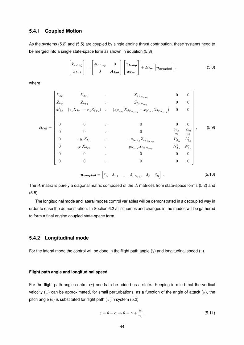
5.4.1 Coupled Motion

As the systems (5.2) and (5.5) are coupled by single engine thrust contribution, these systems need to

be merged into a single state-space form as shown in equation (5.8)xLongxLat

=

ALong 0

0 ALat

xLongxLat

+ Bini

[ucoupled

], (5.8)

where

Bini =

XδE XδT 1... XδTNeng

0 0

ZδE ZδT 1... ZδTNeng 0 0


) ... (zNengXδTNeng− xNengZδTNeng ) 0 0

0 0 ... 0 0 0

0 0 ... 0YδAu0

YδRu0

0 −y1ZδT 1... −yNengZδTNeng L′δA L′δR

0 y1XδT 1... yNengXδTNeng

N ′δA N ′δR

0 0 ... 0 0 0

0 0 ... 0 0 0

, (5.9)

ucoupled =[δE δT 1 ... δTNeng δA δR

]. (5.10)

The A matrix is purely a diagonal matrix composed of the A matrices from state-space forms (5.2) and

(5.5).

The longitudinal mode and lateral modes control variables will be demonstrated in a decoupled way in

order to ease the demonstration. In Section 6.2 all schemes and changes in the modes will be gathered

to form a final engine coupled state-space form.

5.4.2 Longitudinal mode

For the lateral mode the control will be done in the flight path angle (γ) and longitudinal speed (u).

Flight path angle and longitudinal speed

For the flight path angle control (γ) needs to be added as a state. Keeping in mind that the vertical

velocity (w) can be approximated, for small perturbations, as a function of the angle of attack (α), the

pitch angle (θ) is substituted for flight path (γ )in system (5.2)

γ = θ − α→ θ = γ +w

u0. (5.11)

44

The longitudinal space state form transforms now to

xLongγ = ALongγxLongγ + BLongγuLong =Xu Xw − gcos(θ0)

u0−w0 −gcos(θ0)

Zu Zw − gsin(θ0)u0

u0 −gsin(θ0)

Mu Mw + Mθ

u0Mq Mθ

−Zuu0−Zwu0

+ gsin(θ0)u20

0 gsin(θ0)u0

u

w

q

γ

+

XδE XδT 1

... XδTNeng




−ZδEu0

−ZδT 1

u0...

−ZδT Nengu0

uLong . (5.12)

The model in which, longitudinal speed will be controlled is the (5.12), because longitudinal speed is

already an incorporated state in that state-space form.

Final Longitudinal Model

With the expectation of preventing static error on the longitudinal controllable states, two new integrator

states are added.

xu =

∫u dt , xγ =

∫γ dt . (5.13)

These new states, xu and xγ , are respectively integrator states of the longitudinal velocity (u) and flight

path angle (γ). So, the space state (5.12) is now

xLonguγs = ALonguγsxLonguγs + BLonguγsuLong =

Xu Xw − gcos(θ0)u0

−w0 −gcos(θ0) 0 0

Zu Zw − gsin(θ0)u0

u0 −gsin(θ0) 0 0

Mu Mw + Mθ

u0Mq Mθ 0 0

−Zuu0−Zwu0

+ gsin(θ0)u20

0 gsin(θ0)u0

0 0

1 0 0 0 0 0

0 0 0 1 0 0

u

w

q

γ

xu

xγ

+





−ZδEu0

−ZδT 1

u0...

−ZδT Nengu0

0 0 ... 0

0 0 ... 0

uLong . (5.14)

5.4.3 Lateral Mode

Finally, for the lateral mode the control will be done in heading angle (λ).

45

5.4.4 Heading

Only one variable will be controlled in the lateral mode, the heading angle (λ). It can be defined as the

sum of slide slip angle (β) with the yaw angle (ψ)

λ = β + ψ → ψ = λ− β . (5.15)

This will be the fifth lateral state substituting the yaw angle (ψ). The lateral state-space form (5.5) is now

xLatλ = ALatλxLatλ + BLatλuLat =

YβYpu0


u00

L′v L′p L′r 0 0

N ′v N ′p N ′r 0 0

0 1 tan(θ0) 0 0

YβYpu0

+ α01

cos(θ0)+ Yr

u0− 1 gcos(θ0)

u00

β

p

r

φ

λ

+

YδAu0

0 ... 0YδRu0



N ′δR

0 0 ... 0 0YδAu0

0 ... 0YδRu0

uLat .

(5.16)

As in the longitudinal state-space (5.14), a new integrator state is added in order to prevent static error

xλ =

∫λ dt . (5.17)

So state-space form (5.16) transforms into

xLatλs = ALatλsxLatλs + BLatλsuLat =

YβYpu0


u00 0

L′v L′p L′r 0 0 0

N ′v N ′p N ′r 0 0 0

0 1 tan(θ0) 0 0 0

YβYpu0

+ α01

cos(θ0)+ Yr

u0− 1 gcos(θ0)

u00 0

0 0 0 0 1 0

β

p

r

φ

λ

xλ

+

YδAu0

0 ... 0YδRu0



N ′δR

0 0 ... 0 0YδAu0

0 ... 0YδRu0

0 0 ... 0 0

uLat .

(5.18)

5.4.5 Flying and Handling Qualities

Aircraft flying qualities are defined by a number of parameters in the complex frequency domain. In

equation (5.19) there are two of these important parameters, damping ratio (ξ) and undamped natural

frequency (ωn). These parameters depend on the eigenvalue (κ) and having knowledge of these allows

a flight control engineer to imagine the nature of the aircraft’s response to any command or disturbance

[21]. The damping ratio is a dimensionless variable and the natural frequency has its units expressed in

46

radians per second

ωn = |κ|

ξ = −cos(∠κ)(5.19)

On the other hand handling qualities describe the ease with which a pilot can manage an aircraft with

a particular set of flying qualities on a certain mission. It is possible to imagine that the pilot handling

qualities not only depend upon flight qualities but also upon flying controls, the display of flight information

available in the cockpit and among others.

In this dissertation project it is needed to ensure that for a certain mission, the aircraft has the best

flying qualities. The specification used is the MIL-F-8785, Military Specification - Flying Qualities of

Piloted Airplanes published in 1980. The level of flying qualities on this specification depend upon the

aircraft class and flight phase [28].

From the A matrix of state-space systems defined above for both longitudinal and lateral modes

((5.2) and (5.5)), it is possible to establish knowledge of the dynamic stability through its eigenvalues

[21]

det[κI −A] = 0→ |κI −A| = 0 . (5.20)

The I is an identity matrix of the same size of A, the coefficient matrix.

Longitudinal Dynamic Modes

If the eigenvalue equation is applied to the longitudinal coefficient matrix A, a fourth degree polynomial

eigenvalue emerges

κ4 + κ3a1 + κ2a2 + κa3 = 0 . (5.21)

In order to test for the longitudinal dynamic stability of an aircraft, its eigenvalues (κi) must have negative

real parts. If the real part of an eigenvalue is zero or positive, the system’s response to a perturbation

is unstable due to growing oscillations. The equation (5.21) can be factorized into two quadratic factors

such as

(κ2 + 2ξphuωphuκ+ 2ωphu)(κ2 + 2ξspωspκ+ 2ωsp) = 0 . (5.22)

The first factor is relative to a mode of motion which is characterized by an oscillation of long period.

This mode of motion is referred to as the phugoid. It has low frequency (ωphu) and its damping (ξphu) it

is usually low. The second factor is relative to a mode of motion, which is rapid and well-damped. It is

nominated as the short period.

Lateral Dynamic Modes

In the same way of the longitudinal motion, by applying the eigenvalue equation (5.20) to the lateral

coefficient matrix A

κ5 + κ4d1 + κ3d2 + κ2d3 + κd4 = 0 , (5.23)

47

this stability fifth degree equation can be factorized into

κ(κ+ e)(κ+ f)(κ2 + 2ξdrwdrκ+ 2wdr) = 0 . (5.24)

As it is possible to see, κ = 0 is a root of the characteristic equation and that term corresponds to the

heading mode. This means that if the heading is perturbed, there would be no natural tendency for the

aircraft to restore its equilibrium heading. By this is said that an aircraft has neutral heading stability.

The quadratic term in the equation (5.24) is denoted as dutch roll. It usually has a low damping ratio

(ξdr) so that its motion is oscillatory.

The term (κ + e) is referred to spiral mode, which is usually a very slow motion corresponding to a

long term tendency either to maintain the wings level [21].

Finally, the term (κ+ f) is related to the rolling mode which usually is fast.

Level of Flying Qualities

As seen in Table 5.1, there are three levels of performance in the MIL-F-8785, these levels categorize if

the flight qualities are adequate for the mission flight phase,

Level

1 Flying qualities clearly adequate for the mission flight phase

2 Flying qualities adequate to accomplish the mission flight phase, with some increase in pilot

workload or degradation of mission effectiveness

3 Flying qualities such that the aircraft can be controlled safely, but pilot workload is excessive

or mission effectiveness is inadequate

Table 5.1: Aircraft level of perfomance [21]

For this project, it is stipulated that any aircraft for a certain mission must have level 1 of performance

for any mode. In the Chapter 6 it is explained how this goal is achieved.

5.5 Atmospheric Perturbations

An aircraft flying in the atmosphere behaves as a stochastic system due to the system’s noise, external

disturbances and control orders. [12]

Control orders either from the manual pilot or from the automatic flight controller (AFC), noise from

control elements, like sensors, make the system unpredictable and therefore, it is considered stochastic.

Gust perturbations are the external disturbances included in this project. When the air stream is

flowing through the aircraft it’s movements affect the aircraft movement. These disturbances are non-

deterministic and frequently unpredictable. Wind shears, abrupt unpredictable variations of wind speed

through the aircraft, are not having an use in this essay.

48

5.5.1 Influence on the Model

Considering an aircraft entering a zone where there is wind with a given distribution , that is constant

through time but varies in space

ug = ug(x) , (5.25)

vg = vg(x) , (5.26)

wg = wg(x) . (5.27)

The space distribution is transformed through the aircraft displacement in a time distribution

∂v

∂x=

∂v∂t∂x∂t

=1

u0

∂v

∂t. (5.28)

The perturbed motion of the aircraft will result from aerodynamic forces induced by the relative velocity.

Now the air speed (vB), defined in Chapter 3 has to take into account the effect of the wind speed (vW )

vB = v − vW → vB =

u− ugv − vgw − wg

. (5.29)

In the same way, velocity distribution throughout the body of the aircraft also induces an angular velocity

distribution

wB =

p− pgq − qgr − rg

. (5.30)

49

5.5.2 SIMULINK Wind Turbulence Model

The SIMULINK block used to generated wind turbulence is in Figure 5.2. This model generates con-

Figure 5.2: SIMULINK Wind Turbulence Model

tinuous wind turbulence with Dryden velocity spectra. The Dryden turbulence model is mathematically

simplier than von Karman model and it is extensively used in the simulation environment. More informa-

tion about this model is in [29] or in [14]. Inputs for this function are the DCM (NED Direct Cosine Matrix,

A.5), aircraft’s altitude (m) and the magnitude of the velocity vector in the fixed frame. The function also

requires wingspan parameter (b) and allows the user to define the sign of the turbulence angular rates

(q,r). The model outputs the disturbance states for lateral and longitudinal motions (equations (5.32)

and (5.33)).

5.5.3 Disturbances State-space Form

To include the disturbances described above a new state matrix is added into the aircraft dynamics

state-space form (5.1)

x = Ax + Bu + Ed , (5.31)

where d represents the disturbance states and E the associated disturbance influence matrix. Distur-

bance states are distributed according to the mode they belong to, for longitudinal

dLong =[ug wg qg

]T, (5.32)

and for lateral

dLat =[vg pg rg

]T. (5.33)

For the coupled matrix the disturbance states will be

dcoupled =[dLong dLat

]T=

[ug wg qg vg pg rg

]T. (5.34)

The final flight controller state-space with gust disturbances will then be

xcoupled = Acoupledxcoupled + Bcoupleducoupled + Ecoupleddcoupled , (5.35)

50

where

xcoupled =

xLongγxLatλ

, Acoupled =

ALongγ 0

0 ALatλ

. (5.36)

The Bcoupled represents now a 9 × (Neng + 3) driving matrix, being basically a variation of Bini that

includes the driving’s matrix substituted states contribution (ψ for λ and θ for γ)

Bcoupled =


0 0




−ZδEu0

−ZδT 1

u0...

−ZδT Nengu0

0 0

0 0 ... 0YδAu0

YδRu0



N ′δA N ′δR

0 0 ... 0 0 0

0 0 ... 0YδAu0

YδRu0

. (5.37)

The associated disturbance influence 9× 6 matrix for coupled motion, Ecoupled, is

Ecoupled =

−Xu −Xw −Xq 0 0 0

−Zu −Zw −Zq 0 0 0

−Mu −Mw −MwZq 0 0 0

0 0 0 0 0 0

0 0 0 −Yβ −Yp −Yr0 0 0 −L′β −L′p −L′r0 0 0 −N ′β −N ′p −N ′r0 0 0 0 0 0

0 0 0 0 0 0

. (5.38)

51

5.6 SIMULINK State-Space model

The common state-space SIMULINK model could not be used for this project because it does not include

the associated disturbance influence matrix, E. The model in Figure 5.3, satisfies the state-space

equation (5.31). The matrices in Figure 5.3 are the matrices representing the coupled state-space in

Figure 5.3: State-Space model implemented in SIMULINK

equation 5.35. The output matrix, C, is an identity matrix of the same size as the state coefficient matrix,

A, and the direct matrix, D, is a zero matrix of the same size as B.

52

Chapter 6

Optimal Control and Computational

Implementation

In this chapter, the optimal control technique used for the flight controller will be introduced by using an

example of flutter suppression on a two-dimensional aeroelastic airfoil. Then, the approach in which LQR

is going to be utilized in the flight controller is explained. The flight controller module in SIMULINK R© is

demonstrated. At the end of this chapter two important functions that evaluate the level of flying qualities,

are interpreted. The process of choosing an appropriate optimal gain matrix for a general aircraft to be

used in the flight simulation is also described.

6.1 Optimal Control Technique - Linear Quadratic Regulator

Since the flight control problem will be addressed as a linear quadratic problem, an aeroelastic plant with

a LQR (Linear Quadratic Regulator) will be studied. With this study, LQR will be presented and ready

for use on the final flight control problem.

6.1.1 Aeroservoelastic Optimal Control

To introduce the linear quadratic regulator (LQR), a flutter suppression controller of a two-dimensional

aeroelastic airfoil represented in Figure 6.1, will be demonstrated.

53

Figure 6.1: The 2-D cross-section of a airfoil [30]

Though there’s a problem concerning the two-dimensional aeroelastic airfoil equations shown in

Chapter 2. The fundamental equations of this problem are second order, and state-space form first

equation is a first order equation. The mathematical transformation and demonstration of this model is

explained in [30]. The final state space first equation of this model is

x =

A11 A12 A13

A21 A22 A23

A31 A32 A33

Y (t)

Y (t)

xA(t)

+ Bu(t) ,

where the state matrix A is composed of smaller matrices that when complemented form a 10 × 10

matrix. The driving vector B is a 10× 1 matrix, and the state vector is

x =[Y (t) Y (t) xA(t)

]T, (6.1)

where

Y (t) =[h(t)b α(t) β(t)

]T, xA(t) =

[B1(t) B2(t) A1(t) A2(t)

]T. (6.2)

The states are, plunge (h) over time divided by a normalizing constant (b), the pitch over time (α), the

flap angle over time (β), and the aerodynamic lag states (A1(t), A2(t), B1(t), B2(t)). All demonstration of

the sub matrices (Aij) contained in the state coefficient matrix A, aerodynamic lag states and driving

matrix B are in [30], the results were reproduced using the SIMULINK R© tool.

In order to show the effectiveness of the LQR, only the results of the variations over time of the pitch

and the flap angle are going to be considered.

This is a typical aeroservoelastic problem, when the airspeed increases the elastic airfoil starts de-

flecting and therefore increasing the aerodynamic forces acting on it, leading to bigger deflections and

as, a result, bigger oscillations. There is an airspeed limit, called flutter velocity, for marginally stable

oscillations. Depending on the airfoil material, it may lead to a catastrophic structural failure.

54

6.1.2 Open Loop Aeroservoelastic Problem

In this example the flutter velocity (VFlutter) for this airfoil is 297.4 m/s. In order to begin the simulation,

it is considered that there is an initial condition for the state variables (x0).

0 0.5 1 1.5 2 2.5-0.1

-0.05

0

0.05

0.1

Rad

ians

(ra

ds)

Pitch angle α V<Vflutter

Open-loop

0 0.5 1 1.5 2 2.5

Time (s)

-0.05

0

0.05

Rad

ians

(ra

ds)

Flap angle β V<Vflutter

Open-loop

Figure 6.2: Pitch and flap angle variation over time considering (V = 289.6 m/s) on open-loop

Below the flutter velocity, Figure 6.2, it is visible that the larger amplitude oscillations last for about

one second, the system is stable for this airspeed (V ) of 289.6 m/s, all A eigenvalues have real negative

part.

0 0.5 1 1.5 2 2.5-0.1

0

0.1

Rad

ians

(ra

ds)

Pitch angle α V=Vflutter

Open-loop

0 0.5 1 1.5 2 2.5

Time (s)

-0.05

0

0.05

Rad

ians

(ra

ds)

Flap angle β V=Vflutter

Open-loop

Figure 6.3: Pitch and flap angle variation over time considering flutter velocity (V = Vflutter = 297.4 m/s)

on open-loop

If the airspeed is exactly the flutter velocity (V = VFlutter = 297.4 m/s) as in Figure 6.3, the system

remains marginally stable throughout all simulation. Marginally stable means that the matrix A has at

least one eigenvalue with zero real part.

55

0 0.5 1 1.5 2 2.5-0.1

-0.05

0

0.05

0.1

Rad

ians

(ra

ds)

Pitch angle α V>Vflutter

Open-loop

0 0.5 1 1.5 2 2.5

Time (s)

-0.05

0

0.05

Rad

ians

(ra

ds)

Flap angle β V>Vflutter

Open-loop

Figure 6.4: Pitch and flap angle variation over time considering (V = 304.8 m/s) on open-loop

Over the flutter velocity (V = 304.8) m/s, Figure 6.4, the system is clearly unstable, leading the os-

cillations to grow bigger through time. The main cause of the instability of the system is the matrix A

having real positive part eigenvalues. Now the goal is to implement a control law, with the objective to

suppress flutter. This will be done by inducing a feedback gain, calculated by the linear quadratic regu-

lator (LQR), into the system and therefore increasing the system’s flutter velocity. The linear quadratic

regular is used because of its efficient application and utility. There are other more robust control laws,

such as H∞ [31].

6.1.3 Linear Quadratic Regulator

There are two great advantages when solving a linear quadratic problem. Firstly, the control is a full

state linear feedback law

uo = −Kx , (6.3)

and secondly, this resulting feedback control law will ensure the system in closed-loop is stable and ro-

bust, but only if the system is controllable and stabilizable.[21]. This method is based in the optimization

and minimization of the system’s performance index J

J =1

2

∫ ∞0

(xTQx + εuTRu) dt . (6.4)

The equation (6.4) represents a trade-off between, x, u and two matrices Q and R. The state vector x

behaves as a constrain to the minimization of the performance index, J.

Matrices Q and R are square and symmetric matrices and they can be time-dependent. The state

weighting matrix Q is a positive definite matrix and the control cost matrix R is a positive semi-definite

matrix. The objective of these matrices is to regulate the importance of states and inputs variables in the

considered problem. The ε is a parameter that determines the relative weights given to control action

and perturbations in the state variable. It is designated as control penalty parameter.

The resolution of the performance index minimization leads to an optimal gain matrix given by equa-

tion (6.3). This gain affects all states and is considered optimal, given certain matrices Q and R. The

56

demonstration and resolution of the minimization can be seen in [32] or in [14].

In this dissertation, both in this flutter suppression problem and in the final flight controller, MATLAB R©

will be used to generate and solve this linear quadratic problem, using the function lqr. This function uses

the matrix A and B from the state-space form’s first equation, the state weighting matrix Q, the control

cost matrix R and then generates the optimal feedback gain K, known as the gain matrix. This will be

the control method utilized in this project for stabilizing the model and closing the loop.

6.1.4 Closed Loop Aeroservoelastic Problem

In this particular aeroservoelastic case, LQR was applied as a control method in the pursuance of

finding a control function u(t) to stabilize the system. This control function will have the form presented

in equation (6.3)

u(t) = −KLQRx(t) , (6.5)

and the closed loop system

x(t) = Ax(t) + Bu(t) → x(t) = (A−BKLQR)x(t) → x(t) = A∗x(t) , (6.6)

where A∗ is the the augmented plant matrix. The values of the entries of matrices Q and R ((6.7) and

(6.8), respectively) are given through trial and error. The lqr MATLAB R© function retrieves the associated

full state feedback gain accordingly to the system matrices (A and B).

Q =

1000 0 0 0 0 0 0 0 0 0

0 1 0 0 0 0 0 0 0 0

0 0 100 0 0 0 0 0 0 0

0 0 0 1000 0 0 0 0 0 0

0 0 0 0 1 0 0 0 0 0

0 0 0 0 0 100 0 0 0 0

0 0 0 0 0 0 0.1 0 0 0

0 0 0 0 0 0 0 0.1 0 0

0 0 0 0 0 0 0 0 0.1 0

0 0 0 0 0 0 0 0 0 0.1

, (6.7)

R =V 2

1000000. (6.8)

Considering the flutter velocity (Vflutter) as 297.4 m/s, linear quadratic regulator feedback gain for this

arguments will be

KLQR =[0.547 −1.529 0.6858 −38.6409 −39.4681 −27.4179 0.0017 0.0349 0.0001 0.0173

],

(6.9)

and the closed loop pitch and flap angle dynamic response is presented in Figure 6.5.

57

0 0.5 1 1.5 2 2.5-0.1

-0.05

0

0.05

0.1

Rad

ians

(ra

ds)

Pitch angle α V=Vflutter

Closed-loop LQR

0 0.5 1 1.5 2 2.5

Time (s)

-0.05

0

0.05

Rad

ians

(ra

ds)

Flap angle β V=Vflutter

Closed-loop LQR

Figure 6.5: Pitch and flap angle variation over time considering flutter velocity (V = Vflutter = 297.4 m/s)

on closed-loop

It is possible to see that closing the loop stabilized the system. This system that once was marginally

stable on the open-loop, now is completely stable having its oscillations ending after about one and a

half seconds. The full state feedback gain made the zero real part eigenvalues of open-loop, translate

to real negative part eigenvalues in the closed loop.

Applying the same method but for an airspeed of 304.8 m/s, that in the open loop would make the

system unstable. The full state feedback gain will be

KLQR =[9.8 −39.9 −1.6 −1279.7 −804 −650.2 0.1 0.9 0 0.1

], (6.10)

and the following closed loop pitch and flap angle dynamic response is presented in Figure 6.6.

0 0.5 1 1.5 2 2.5-0.1

-0.05

0

0.05

0.1

Rad

ians

(ra

ds)

Pitch angle α V>Vflutter

Closed-loop LQR

0 0.5 1 1.5 2 2.5

Time (s)

-0.05

0

0.05

Rad

ians

(ra

ds)

Flap angle β V>Vflutter

Closed-loop LQR

Figure 6.6: Pitch and flap angle variation over time considering (V = 304.8 m/s) on closed-loop

This open-loop unstable system is now stable in the closed loop having its oscillations end after

about one second. The closed loop eigenvalues both in this case and on the case above, all have real

negative parts.

58

6.1.5 Linear Quadratic Regulator Concerns and Conclusions

However through these two examples it is possible to see that suppressing flutter for higher airspeed

using the LQR method implies higher gain matrices, or in this case, gain vectors. There is also one

final thought to add to this particular problem, there is not a control variable in it. This is a merely

mathematical demonstration of the LQR virtues, the control vector (u) in this problem is always the

feedback gain from LQR.

Summing up, LQR control is tempting but unrealistic. Firstly because it needs all states to be known

at all times in order to use state feedback. In this particular case it would be impractical since some

of the states, as aerodynamic lag states (A1(t), A2(t), B1(t) and B2(t)), are not physical and therefore

cannot be detected by sensors. Secondly, for higher airspeed, LQR produces higher gains, and in the

real world, actuators may not be able to deal with these higher gains, resulting in saturation. However,

it is an easy implementable and robust control tool, and it will be the control method adopted in this

dissertation’s flight controller.

One of the problems for this thesis project is the definition of the LQR weight matrices (Q and R). In

the flutter suppression problem, these matrices were defined arbitrarily, through trial and error, with the

objective to have the best possible full state feedback gain [30]. Although in the flight controller, as it will

be for a generic aircraft on a given flight condition, a method for obtaining appropriate state weighting

(Q) and control cost (R) matrices is required.

Bryson’s Method

Since the definition of matrices Q and R can be arbitrary, there is a method called Bryson’s method

in which it suggests that each term of the diagonal matrices, Q and R, is the inverse square of the

maximum value expected for the variable on the simulation time. As it follows

Q = diag(Qi)⇒ Qi =1

x2imax, R = diag(Ri)⇒ Ri =

1

u2imax. (6.11)

In the flight control system, u2imax and x2imax are the values indicating the extreme of the perturbations

wanted for ui or xi for the closed loop during a maneuver. This method is a good starting point to define

these matrices and will be used in the flight control problem. [14]

59

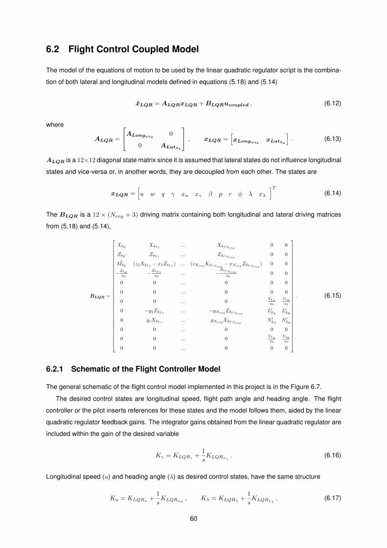
6.2 Flight Control Coupled Model

The model of the equations of motion to be used by the linear quadratic regulator script is the combina-

tion of both lateral and longitudinal models defined in equations (5.18) and (5.14)

xLQR = ALQRxLQR + BLQRucoupled , (6.12)

where

ALQR =

ALonguγs 0

0 ALatλs

, xLQR =[xLonguγs xLatλs

]. (6.13)

ALQR is a 12×12 diagonal state matrix since it is assumed that lateral states do not influence longitudinal

states and vice-versa or, in another words, they are decoupled from each other. The states are

xLQR =[u w q γ xu xγ β p r φ λ xλ

]T(6.14)

The BLQR is a 12 × (Neng + 3) driving matrix containing both longitudinal and lateral driving matrices

from (5.18) and (5.14),

BLQR =


0 0




−ZδEu0−ZδT 1

u0... −

ZδT Nengu0

0 0

0 0 ... 0 0 0

0 0 ... 0 0 0

0 0 ... 0YδAu0

YδRu0



N ′δA N ′δR

0 0 ... 0 0 0

0 0 ... 0YδAu0

YδRu0

0 0 ... 0 0 0

. (6.15)

6.2.1 Schematic of the Flight Controller Model

The general schematic of the flight control model implemented in this project is in the Figure 6.7.

The desired control states are longitudinal speed, flight path angle and heading angle. The flight

controller or the pilot inserts references for these states and the model follows them, aided by the linear

quadratic regulator feedback gains. The integrator gains obtained from the linear quadratic regulator are

included within the gain of the desired variable

Kγ = KLQRγ +1

sKLQRxγ

. (6.16)

Longitudinal speed (u) and heading angle (λ) as desired control states, have the same structure

Ku = KLQRu +1

sKLQRxu

, Kλ = KLQRλ +1

sKLQRxλ

. (6.17)

60

Figure 6.7: Schematic of the control law

The integrator states variables eliminate constant input values and also helps to stabilize the system. All

of these gains are optimal and are calculated using the Bryson’s method explained in Section 6.1.5. The

non-desired control state gains, Kw,q,β,p,r,φ, are included in the outer feedback loop, as seen in Figure

6.7

Kw,q,β,p,r,φ =[KLQRw KLQRq KLQRβ KLQRp KLQRr KLQRφ

]T. (6.18)

The input vector will then be

u = −[Ku Kγ Kλ

]u− urefγ − γrefλ− λref

− [KLQRw KLQRq KLQRβ KLQRp KLQRr KLQRφ

]

w

q

β

p

r

φ

(6.19)

61

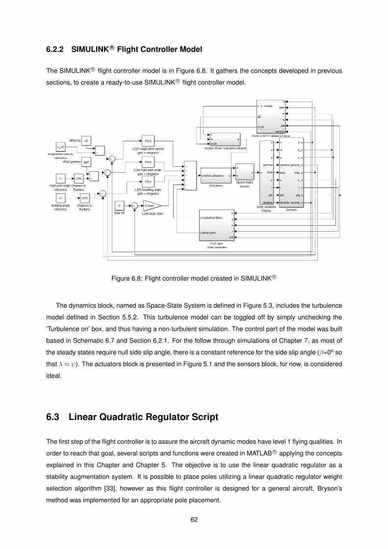
6.2.2 SIMULINK R© Flight Controller Model

The SIMULINK R© flight controller model is in Figure 6.8. It gathers the concepts developed in previous

sections, to create a ready-to-use SIMULINK R© flight controller model.

Figure 6.8: Flight controller model created in SIMULINK R©

The dynamics block, named as Space-State System is defined in Figure 5.3, includes the turbulence

model defined in Section 5.5.2. This turbulence model can be toggled off by simply unchecking the

’Turbulence on’ box, and thus having a non-turbulent simulation. The control part of the model was built

based in Schematic 6.7 and Section 6.2.1. For the follow through simulations of Chapter 7, as most of

the steady states require null side slip angle, there is a constant reference for the side slip angle (β=0o so

that λ ≈ ψ). The actuators block is presented in Figure 5.1 and the sensors block, for now, is considered

ideal.

6.3 Linear Quadratic Regulator Script

The first step of the flight controller is to assure the aircraft dynamic modes have level 1 flying qualities. In

order to reach that goal, several scripts and functions were created in MATLAB R© applying the concepts

explained in this Chapter and Chapter 5. The objective is to use the linear quadratic regulator as a

stability augmentation system. It is possible to place poles utilizing a linear quadratic regulator weight

selection algorithm [33], however as this flight controller is designed for a general aircraft, Bryson’s

method was implemented for an appropriate pole placement.

62

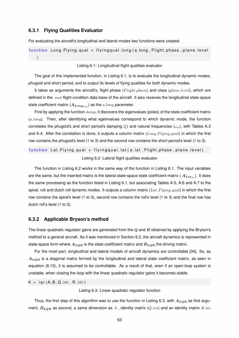
6.3.1 Flying Qualities Evaluator

For evaluating the aircraft’s longitudinal and lateral modes two functions were created.

f u n c t i o n Long F ly ing qua l = f l y i n g q u a l l o n g ( a long , F l igh t phase , p l a n e l e v e l

)

Listing 6.1: Longitudinal flight qualities evaluator

The goal of this implemented function, in Listing 6.1, is to evaluate the longitudinal dynamic modes,

phugoid and short period, and to output its levels of flying qualities for both dynamic modes.

It takes as arguments the aircraft’s, flight phase (Flight phase) and class (plane level), which are

defined in the .mat flight condition data base of the aircraft. It also receives the longitudinal state-space

state coefficient matrix (ALonguγs ) as the a long parameter.

First by applying the function damp, it discovers the eigenvalues (poles) of the state coefficient matrix

(a long). Then, after identifying what egeinvalues correspond to which dynamic mode, the function

correlates the phugoid’s and short period’s damping (ξ) and natural frequencies (ωn), with Tables A.3

and A.4. After the correlation is done, it outputs a column matrix (Long F lying qual) in which the first

row contains the phugoid’s level (1 to 3) and the second row contains the short period’s level (1 to 3).

f u n c t i o n L a t F l y i n g q u a l = f l y i n g q u a l l a t ( a l a t , F l igh t phase , p l a n e l e v e l )

Listing 6.2: Lateral flight qualities evaluator

The function in Listing 6.2 works in the same way of the function in Listing 6.1. The input variables

are the same, but the inserted matrix is the lateral state-space state coefficient matrix ( ALatλs ). It does

the same processing as the function listed in Listing 6.1, but associating Tables A.5, A.6 and A.7 to the

spiral, roll and dutch roll dynamic modes. It outputs a column matrix (Lat F lying qual) in which the first

row contains the spiral’s level (1 to 3), second row contains the roll’s level (1 to 3) and the final row has

dutch roll’s level (1 to 3).

6.3.2 Applicable Bryson’s method

The linear quadratic regulator gains are generated from the Q and R obtained by applying the Bryson’s

method to a general aircraft. As it was mentioned in Section 6.2, the aircraft dynamics is represented in

state-space form where ALQR is the state coefficient matrix and BLQR the driving matrix.

For the most part, longitudinal and lateral models of aircraft dynamics are controllable [34]. So, as

ALQR is a diagonal matrix formed by the longitudinal and lateral state coefficient matrix, as seen in

equation (6.13), it is assumed to be controllable. As a result of that, even if an open-loop system is

unstable, when closing the loop with the linear quadratic regulator gains it becomes stable.

K = l q r (A,B, Q in i , R i n i )

Listing 6.3: Linear quadratic regulator function

Thus, the first step of this algorithm was to use the function in Listing 6.3, with ALQR as first argu-

ment, BLQR as second, a same dimension as A , identity matrix (Q ini) and an identity matrix R ini

63

with dimension equal to the columns of BLQR (number of control variables). The augmented plant

matrix (closed loop) of equation (6.20)

A∗LQR = ALQR −BLQRK , (6.20)

is guaranteed to be stable. The A∗LQR and BLQR matrices are then used as the state coefficient matrix

and driving matrix, respectively, in the state-space of Figure 6.9. It was chosen for the impulses of the

control surfaces in Figure 6.9, 10% of the maximum surface deflections, as it represents, for a general

aircraft, the control surface deflection used in a typical manoeuvre. The Bryson’s method Rfinal matrix

will be a diagonal matrix composed of the inverse-square of these values ( 1u2imax

).

Figure 6.9: SIMULINK R© schematic used for applying Bryson’s Method (Neng = 2)

Covering all combinations of impulses on the control surfaces, the script saves the state maximum

values obtained by the various simulations for each state variable. Those values (ximax ) are then used

to create the Bryson’s method Qfinal matrix, which will be a diagonal state matrix with entries, 1x2imax

,

that are relative to each state.

With these new Qfinal and Rfinal matrices, there’s a cycle, that tests for each iteration the flying

qualities of the aircraft in the closed loop. In each iteration the Rfinal matrix is multiplied by a certain

control penalty parameter (ε varies from 0.1 to 1000) and then submitted to the lqr function of Listing

6.4. The cycle breaks when the script finds an augmented matrix

A∗LQR = ALQR −BLQRKLQR , (6.21)

64

that has level 1 qualities in all dynamic modes. Therefore for each iteration, functions in Listings 6.2 and

6.1 are consecutively called to check the augmented matrix lateral and longitudinal dynamics’ modes

levels. Briefly, when the cycle breaks it means the optimal gain matrix (KLQR) to use in the flight

controller is found.

K LQR = l q r (A LQR, B LQR, Q f i na l , R f i n a l ∗ rho )

Listing 6.4: Linear quadratic regulator function cycle

65

Chapter 7

Flight Simulation

Besides the flight dynamics integrator program created in C++ R©, an optimal flight controller using LQR

on MATLAB R© was also developed. This program made of the MATLAB R© scripts and SIMULINK mod-

ules, seen over Chapters 6 and 5, will allow the study of certain flight conditions from a flight engineer

point of view.

Initially, open-loop dynamics of the flight conditions for the Airbus A400M and the Dassault Falcon

7X aircraft will be analysed. Then, the goal is to use the flight controller to follow a reference in the case

of engine failure and turbulence.

7.1 Open-Loop Dynamics

The aircraft used for the engine failure test is the four engines Airbus A400M and the aircraft to be tested

in turbulent flow is the Dassault Falcon 7X . These aircraft trim data is in Appendix A.3.3.

AircraftDassault Falcon 7X Airbus A400M

Longitudinalmotion

Phugoid κphu1= -0.0579 + 0.231i

κphu2=-0.0579 - 0.231i

κphu1= -0.066 +0.0883i

κphu2= -0.066 - 0.0883i

Short period κsp1 = -0.7270 + 1.5iκsp2 = -0.7270 + 1.5i

κsp1= -7.47 + 3.23iκsp1 = -7.47 - 3.23i

Lateralmotion

Spiral κspi =-0.0138 κspi = 0.0840Roll κroll = -2.35 κroll = -1.26

Dutch Roll κdr1 = -0.314 + 4.18iκdr2 = -0.314 - 4.18i

κdr1 = -0.141 + 1.82iκdr2 = -0.141 - 1.82i

Heading mode κλ = 0 κλ = 0

Table 7.1: Open-loop dynamic modes eigenvalues

By first applying equation (5.19) and then correlating the damping and the natural frequency of

A400M dynamic modes, contained in Table 7.1, with Tables A.3, A.4, A.6, A.5 and A.7. It is possi-

ble to conclude that the phugoid has level three and the short period has level two. In the lateral motion,

the spiral mode is stable and thus level one, roll is also level one and dutch roll is categorized as level

two. The pole at the origin is due to the heading mode (λ), seen in Section 5.4.5. Overall, the longitudinal

and lateral motions of the aircraft do not have the level one flying qualities requirement.

67

When categorizing the dynamic modes of the Dassault Falcon 7X, utilizing the same method as

above, phugoid is level one and the short period is also level one. As for the lateral dynamic modes,

spiral is a positive real number making it level three, however roll is level one and dutch roll is level two.

Dynamic modes of this Falcon 7X’s flight condition are unstable.

The LQR script of Chapter 6 must place the poles of these dynamic modes, in order that the level

one flying qualities of the aircraft are satisfied.

7.2 Engine Failure

In this section, the left engines of the four engine Airbus A400M (δT1and δT2

) are malfunctioning and

therefore providing no thrust to the aircraft

δT1= 0 , δT2

= 0 . (7.1)

The control surfaces available for the aircraft are then δT3, δT4

, δE , δA and δR. The goal is to perform

a climb (γref = 1o) while maintaining heading (λref = 0o). The reference for longitudinal velocity is

maintained at the trim velocity (uref = u0).

First, the state coefficient matrices (Acoupled to be used in the state-space and ALQR in the linear

quadratic regulator script) and driving matrices (Bcoupled to be used in the state-space and BLQR in the

linear quadratic regulator script) need to be defined by utilizing the A400M trim condition data contained

in Appendix A.3.3.

The script is then called and proceeds to find level one flying qualities for a control penalty parameter

of ε = 10. In the gain matrix associated with this value (B.9), the two rows composed of zeros correspond

to engine one (δT1 ) and engine two (δT2 ), which are not functioning.

Control penalty parameter (ε) 10 40 80

Longitudinal

motion

Phugoid

(κphu1,2)

-0.597 ± 0.252i -0.414 ± 0.36i -0.369 ± 0.36i

Short period

(κsp1,2 )-11.3 ± 4.37i -6.86 ± 5.23i -5.39 ± 4.92i

Lateral

motion

Spiral

(κspi)-0.631 -0.603 -0.569

Roll

(κroll)-3.36 -2.54 -2.28

Dutch roll

(κdr1,2 )-1.98 ± 2.65i -1.33 ± 2.41i -1.08 ± 2.26i

Table 7.2: Closed loop poles for ε = 10, ε = 40 and ε = 80

The closed-loop dynamic mode poles are represented in Table 7.2. Upon initial inspection, the poles

are moving to the right side of the complex plane as the control penalty paramenter (ε) is increasing.

68

Thus, this parameter, as it is penalizing the control input, when assigned high values can make the

open-loop and closed-loop dynamic responses be virtually identical.

The model’s dynamic responses of a thirty five seconds simulation on SIMULINK are presented in

Figures 7.1, 7.2 and 7.3. The position of the aircraft in the ENU frame is defined in Figure 7.4. Three

different control penalty parameters were tested, in order to see its influence in the aircraft dynamics.

Therefore, for each plot there are three sets of curves and the markers for each curve are only to

ease identification. In Figures 7.1 and 7.2, the effects of the control penalty parameter on the control

0 5 10 15 20 25 30 35tseconds

-10

0

10

δE (

º)

Elevator angle ( δE) (º)

ǫ = 10ǫ = 40ǫ = 80

0 5 10 15 20 25 30 35tseconds

-5

0

5

δR

(º)

Rudder angle ( δR

) (º)

0 5 10 15 20 25 30 35tseconds

-4

-2

0

2

4

δA (

º)

Aileron angle ( δA

) (º)

Figure 7.1: Dynamic responses of the control input variables (δE ,δA,δR) for three different control penaltyparameters

surfaces dynamic responses are evident. Dynamic responses of engines 1 and 2 (δT1 and δT2 ) are not

represented as their response is zero over the whole simulation. When the system has reached an

equilibrium state, the constant negative deflections in the rudder and ailerons generate a positive yaw

and clockwise roll moments used to stabilize the aircraft due to the loss of the two left engines. As

the aircraft also needs to climb (γref = 1o), after the initial variations, the elevator deflection finds its

equilibrium state at a negative value. As the functioning engines have influence in the longitudinal and

lateral motion, the outer engine throttle (δT4) tends to decrease because of its higher influence in the yaw

moment, and the inner engine (δT3 ) increases its thrust in such a way that the three reference states are

achievable and an equilibrium state is found.

Increasing the control penalty parameter makes the system utilize less the control surfaces, therefore

69

0 5 10 15 20 25 30 35tseconds

0

20

40

60

80

100δ

T3

(%

)

Throttle (δT

3

) (%)

ǫ = 10ǫ = 40ǫ = 80

0 5 10 15 20 25 30 35tseconds

0

10

20

30

40

δT

4

(%

)

Throttle (δT

4

) (%)

Figure 7.2: Dynamic responses of the non-malfunctioning engines (δT3,δT4

) for three different controlpenalty parameters

reaching the desirable state in a higher time. However, higher values also attenuates the overshooting

deflections when requested to follow a reference, making the system more realistic, because high over-

shooting deflections in control surfaces in short periods of time may have rough effects in the aircraft

structural dynamics. These overshooting control surfaces deflections also may not be physically possible

due to the actuator dynamics.

When the system allows for higher control deflections (ε = 10), the reference state is reached faster

than when the control action is more limited (ε = 80). However, for reasonable values of ε and assuming

the system is stable, this final reference state is eventually reached as seen in Figure 7.3.

The representation of the states transformed into positions on the XYENU and Y ZENU planes are

shown in 7.4. The aircraft’s trajectory is represented in the ENU reference frame, to facilitate visual

interpretation of the results. Initially the lack of thrust in the left engines make the aircraft deviate to the

left (negative xENU ) but eventually through the control surfaces deflections the heading is stabilized.

For this case in specific the handling qualities might arise due to ωphuωsp

being always less than 0.1,

however the reason for this is the malfunctioning of the two engines. For this trim condition data after

level one flying qualities is achieved (ε = 10), the result of that division is always decreasing for higher ε

values, making it impossible to reach.

70

0 5 10 15 20 25 30 35tseconds

0

0.5

1

γ (

º)

Flight path angle, γ (º)

ǫ = 10ǫ = 40ǫ = 80

0 5 10 15 20 25 30 35tseconds

-3

-2

-1

0

λ (

º)

Heading angle, λ (º)

0 5 10 15 20 25 30 35tseconds

140.8

141

141.2

u (m

/s)

Velocity u (m/s)

Figure 7.3: Dynamic responses of the controllable states (u,γ,λ)

0 500 1000 1500 2000 2500 3000 3500 4000 4500 5000y

ENU (m)

-80

-60

-40

-20

0

x EN

U (

m)

XY Plane

ǫ = 10ǫ = 40ǫ = 80

0 500 1000 1500 2000 2500 3000 3500 4000 4500 5000y

ENU (m)

1000

1020

1040

1060

1080

1100

z EN

U

YZ Plane

Figure 7.4: Flight trajectory seen in XYENU and Y ZENU planes (γref = 1o, λref = 0o and uref = u0)

71

7.3 Turbulence

In this Section the three engined Dassault Falcon 7X aircraft is flying in a turbulent flow. The aircraft is

required to maintain its heading and flight path angle (λref = γref = 0o), all of the three engines are

functioning. The state coefficient (A) and driving (B) matrices are determined by utilizing the aircraft’s

trim condition data contained in Appendix A.3.3.

The first control penalty parameter for which the script found level one flying qualities was for ε = 20.

The gain matrix represented in equation B.10, has the particularity of its middle engine only affecting

the longitudinal mode, as it is situated under the elevator and thus, has no influence in the yaw and roll

moment.

Alongside with the control penalty parameter found by the script, two more dynamic responses pro-

duced by other two control parameters are analysed. This time, a higher and lower order of magnitude

values were used. The high order value (ε = 200) has level one flying qualities and the lower order value

does not have level one flying qualities.

Control penalty (ε) 2 20 200

Longitudinal

motion

Phugoid

(κphu1,2)

κphu1=-2.34

κphu2=-0.591

-0.306 ± 0.241i -0.266 ± 0.424i

Short period

(κsp1,2 )-8.28 ± 0.65i -2.82 ± 3.52i -1.71 ± 1.99i

Lateral

motion

Spiral

(κspi)-0.792 -0.620 -0.435

Roll

(κroll)-4.40 -2.75 -2.45

Dutch roll

(κdr1,2 )

κdr1 =-14.7

κdr2 =-2.54-2.83 ± 3.51i -0.951 ± 4.11i

Table 7.3: Closed loop poles for ε = 2, ε = 20 and ε = 200

In Table 7.3, the poles for different control penalty parameters are represented. For the lower value

of control penalty the phugoid and dutch roll dynamic modes are critically damped, such value is not

adequate for a realistic and practical system. Overall the poles behave the same way with the control

penalty parameter as in Table 7.2.

Just as in Section 7.2, there are three curves for each plot, each representing a control penalty value.

In Figures 7.5, 7.6 and 7.7 there are the dynamic responses and Figure 7.8 has the positions during the

thirty five seconds simulation.

In Figure 7.5, as the objective is the aircraft maintaining its altitude (γref = 0o) and heading (λref =

0o), for the values of control penalty parameter computed, the goal is achieved. The control penalty

analysis is somewhat similar to the engine failure situation of Section 7.2, for higher values its control

system is weighting heavily in the performance index, making the aircraft having larger deviations due

to turbulence.

72

0 5 10 15 20 25 30 35tseconds

-4

-2

0

2

γ (

º)

Flight path angle, γ (º)

ǫ = 20ǫ = 2ǫ = 200

0 5 10 15 20 25 30 35tseconds

-2

0

2

λ (

º)

Heading angle, λ (º)

0 5 10 15 20 25 30 35tseconds

46.5

47

47.5

48

u (m

/s)

Velocity u (m/s)

Figure 7.5: Dynamic responses of the controllable states (u,γ,λ)

The interpretation of Figures 7.6 and 7.7 is also identical to the control surfaces deflections in Section

7.2. With higher values of control penalty parameter, the control surfaces are susceptible of having

higher deflections to reach its reference state. On the other hand, for lower values it is more sensitive

and tends to saturate its control inputs more often (δT1and δT3

).

The level of turbulence used in the Dryden model was categorized as ”Moderate” and its turbulence

angular rates (q,r) are characterized as positive. The reference frame used was also the ENU. During

the flight trajectory, the aircraft is seriously effected by turbulence, having its route oscillate significant

values. For this aircraft’s flight condition and for ε = 20 or ε = 200, there should not be a problem with

handling qualities as ωphuωsp

is greater than 0.1 for both cases. The lower order of magnitude ε = 2 has

critically damped modes and so it was concluded that for lower control penalty parameter values (ε) the

dynamic responses are impractical and unrealistic.

Summing up, it is safe to say that for the less penalized control system, as it weighs less in the

performance index, it has a better overall dynamic response but at a higher control cost. As this script

is supposed to work for any general engined aircraft, it finds the less penalized, by performance index,

control system which has level one flying qualities. Sometimes it can be adequate to the aircraft flight

condition, sometimes it cannot.

73

0 5 10 15 20 25 30 35tseconds

-4

-2

0

2

4

δE (

º)

Elevator angle ( δE) (º)

ǫ = 20ǫ = 2ǫ = 200

0 5 10 15 20 25 30 35tseconds

-2

0

2

δR

(º)

Rudder angle ( δR

) (º)

0 5 10 15 20 25 30 35tseconds

-4

-2

0

2

4

δA (

º)

Aileron angle ( δA

) (º)

Figure 7.6: Dynamic responses of the input variables (δE ,δA,δR)

74

0 5 10 15 20 25 30 35tseconds

60

80

100δ

T1

(%

)Throttle (δ

T1

) (%)

ǫ = 20ǫ = 2ǫ = 200

0 5 10 15 20 25 30 35tseconds

60

80

100

δT

2

(%

)

Throttle (δT

2

) (%)

0 5 10 15 20 25 30 35tseconds

60

80

100

δT

3

(%

)

Throttle (δT

3

) (%)

Figure 7.7: Dynamic responses of the engines (δT1,δT2

,δT3)

0 200 400 600 800 1000 1200 1400 1600y

ENU (m)

-5

0

5

x EN

U (

m)

XY Plane

ǫ = 20ǫ = 2ǫ = 200

0 200 400 600 800 1000 1200 1400 1600y

ENU (m)

1490

1495

1500

1505

1510

1515

z EN

U (

m)

YZ Plane

Figure 7.8: Turbulent flight trajectory seen in XYENU and Y ZENU planes (γref = 1o, λref = 0o anduref = u0)

75

Chapter 8

Conclusions

This dissertation not only developed a crucial piece for a future aeroservoelastic tool but also a flight

controller that can possibly be embedded into it.

The integrator results depend highly on the stepper used. For aircraft with low and medium ma-

noeuvrability, an error stepper is recommended, although for high manoeuvrability aircraft a controlled

stepper is the one to use as a result of overshooting responses and high variations in short periods of

time.

The defined trim condition aeroservoelastic mathematical equations of motion are also left in a gen-

eral state, as it is difficult to define the number of vibration modes required. This number of vibration

modes rely upon not only on the approximation needed to define the structural influence on flight dy-

namics, but also on the aircraft to be studied.

The flight controller simulations and mathematical model results were as expected. However, the

linear quadratic regulator as the control law is not always practical, serving nevertheless good use when

designing a control tool for a general aircraft as in this dissertation. The flight simulator realizes the

simulation based on the first control penalty parameter (ε) found that has level one flying qualities. For

certain flight conditions it might not be the most appropriate, as it might cause overshooting and therefore

create unrealistic simulations.

8.1 Achievements

During the present work I was able to accomplish the majority of the proposed objectives. The math-

ematical elastic equations of motion were successfully demonstrated for a equilibrium condition of a

general aircraft.

Then, these equations were implemented as a C++ R© program which integrates these equations for

a time interval (∆t), different integration techniques were also analysed for a practical case.

The flight simulator was successfully built, the implementation of control laws on the dynamics model.

However, it was not possible to simulate using structural vibration modes due to lack of data about

these. Two different simulations for two different aircraft were carried out in MATLAB R© and SIMULINK R©

77

environments, and with these simulations significant results, about the control method used and flight

dynamics, were obtained.

8.2 Future Work

There is no doubt that the purpose of this work is to have continuation. The flight dynamics integrator

is going to work as a fundamental role by functioning as a bridge between several disciplines such as

aerodynamics, structures and control. The way these connections are going to be made is open to the

user. The flight dynamics integrator observer argument has many possible diverse uses, in the manner

that it can be used to write on a file, for interprocess communication, serial port writing, among others.

The flight dynamics integrator is ready to receive the necessitated values of other programs, however

it is only doing one integration. The future use that is given to the flight dynamics integrator needs to

take into account the recursivity, the program is left in its simplest state, only realizing one integration, to

allow the future user to change it according to his objectives.

The flight dynamics integrator stepper was used based on one flight condition integration. When

using it, it is important to take in consideration the stepper and the integration time interval, in order to

gather adequate results.

The mathematical trim equations of motion for an aeroservoelastic model were also deduced, giving

the possibility to be included in other projects or developed even more.

The idea of building a flight controller and a flight dynamics integrator for a general aircraft, made

this dissertation a bit generalist and hard to, for instance, include sensors and structural data into the

simulations. So, a future idea is also to concentrate on a certain aircraft, and build a full aeroservoelastic

flight controller with different missions and manoeuvres by embedding the aeroelasticity characteristics

in this flight control simulation tool.

Another interesting concept is create general structural dynamics and aerodynamics models and

through the flight dynamics integrator test new aircraft designs and possibilities, in such way, the aeroser-

voelastic simulator would work as a research simulator.

78

Bibliography

[1] R. Bisplinghoff and H. Ashley. Principles of Aeroelasticity. Dover Phoenix Editions, 2002.

[2] A. R. Collar. The first fifty years of aeroelasticity, 1978.

[3] M. L. Baker, P. J. Goggin, and B. A. Winther. Aeroservoelastic modeling, analysis, and design

techniques for transport aircraft. In Structural Aspects of Flexible Aircraft Control, 2000.

[4] M. Karpel. Procedures and models for aeroservoelastic analysis and design. ZAMM - Journal of

Applied Mathematics and Mechanics, 2001.

[5] D. Allerton. Principles of flight simulation. Wiley, 2009.

[6] S. K. Advani. The Kinematic Design of Flight Simulator Motion-Bases. Delf University Press, 1998.

[7] J. R. Wright and J. E. Cooper. Introduction to Aircraft Aeroelasticiy and Loads. Wiley, 2007.

[8] D. L. York. Analysis of flutter and flutter suppression via an energy method. Master’s thesis, Virgina

Polytechnic Institute and State University, 1980.

[9] A. Tewari. Aeroservoelasticity Modeling and Control. Springer, 2015.

[10] R. Blockley and W. Shyy. Encyclopedia of Aerospace Engineering. Wiley, 2010.

[11] Y. C. Fung. An Introduction to the theory of aeroelasticity. John Wiley and Sons, 1955.

[12] J. Oliveira. Apontamentos de estabilidade de voo. Instituto Superior Tecnico, 2013.

[13] H. Farrell and M. Barth. The Global Positioning System and Inertial Navigation. McGraw, 1999.

[14] J. Azinheira. Apontamentos de controlo de voo. Instituto Superior Tecnico, 2013.

[15] P. Singla, D. Mortari, and J. Junkins. How to avoid singularity when using euler angles? Available

online: http://lairs.eng.buffalo.edu/pdffiles/pconf/C10.pdf.

[16] F. P. Beer and E. R. Johnston. Vector Mechanics for Engineers Dynamics. McGraw-Hill, 2006.

[17] C. W. de Silva. Sensors and Actuators: Engineering System Instrumentation. CRC Press, 2015.

[18] E. Haskel. http://code7700.com/drag.html. Code 7700.

[19] B. Etkin. Dynamics of Atmosferic Flight. Dover Phoenix Editions, 2005.

79

[20] E. D. Achtmann. A critical review of world jet transport safety. Master’s thesis, Massachusetts

Institute of Technology, 1995.

[21] D. McClean. Automatic Flight Control Systems. Granada Publishing Limited, 1979.

[22] M. R. Waszak, J. B. Davidson, and D. K. Schmidt. A Simulation Study of the Flight Dynamics of

Elastic Aircraft. NASA, 1987.

[23] R. D. Milne. Dynamics of the deformable aeroplane. Technical report, British Aeronautical Research

Council, 1964.

[24] B. Raghavan. Flight Dynamics and Control of Highly Flexible Flying-Wings. PhD thesis, Faculty of

the Virginia Polytechnic Institute and State University, 2009.

[25] R. C. Schwanz. Formulations of the equations of motion of an elastic aircraft for stability and flight

control applications. Technical report, Airforce Flight Dynamics Laboratory, 1972.

[26] K. Ahnert and M. Mulansky. http://www.boost.org/doc/libs/. Boost C++ libraries.

[27] A. Klein and A. Godunov. Introductory Computational Physics. Cambridge University Press, 2006.

[28] MIL-F-8785. Military Specification - Flying Qualities of Piloted Airplanes. American Department of

Defense, 1980.

[29] M. V. Cook. Flight Dynamics Principles: A Linear Systems Approach to Aircraft Stability and Control.

Butterworth-Heinemann, 2013.

[30] S. D. Olds. Modeling and lqr control of a two-dimensional airfoil. Master’s thesis, Virgina Polytechnic

Institute and State University, 1997.

[31] J. Theis. Robust control design for active flutter suppression. Master’s thesis, University of Min-

nesota, 2016.

[32] A. Tewari. Modern Control Design With MATLAB and SIMULINK. Wiley, 2002.

[33] J. D. Robinson. A linear quadratic regulator weight selection algorithm. Master’s thesis, Air Force

Institute of Technology, 1990.

[34] R. Stengel. Flight Dynamics. Princeton University Press, 2004.

[35] J. Azinheira. Controlo de voo, enunciado dos projectos 2013-2014. Controlo de Voo, 2014.

80

Appendix A

Reference Frames, Stability

Derivatives, Flying Qualities and Trim

condition Aircraft data

A.1 Rotation Matrices

In order to be able to relate vectors from one reference frame to another, rotation matrices have to be

introduced. Basically rotation matrices transform the components of a vector from a axis system to

another.

In this section A.1, first the rotation matrices of three generalized axis sytem, and three angles will

be defined. After this step is done the goal is reaching the final rotation matrix.

Figure A.1: Rotations around each of the generalized axis systems [12]

For one rotation of an angle α over the x-axis, the rotation matrix Lx is,

Lx(α) =

1 0 0

0 cos(α) sin(α)

0 −sin(α) cos(α)

, (A.1)

rotation of an angle β over the y-axis, the rotation matrix Ly is,

81

Ly(β) =

cos(β) 0 −sin(β)

0 1 0

sin(β) 0 cos(β)

, (A.2)

and finally the rotation of an angle γ over the z-axis, the rotation matrix Lz is,

Lz(γ) =

cos(γ) sin(γ) 0

−sin(γ) cos(γ) 0

0 0 1

. (A.3)

The rotation matrix of the fixed reference frame,FE , to the body reference frame, FB , is the multiplica-

tion (right to left) of the single rotation matrices corresponding to the Euler angles (Lx(φ),Ly(θ),Lz(ψ)).

LBE = Lx(φ)Ly(θ)Lz(ψ) (A.4)

LBE =

cos(θ)cos(ψ) cos(θ)sin(ψ) −sin(θ)

sin(φ)sin(θ)cos(ψ)− cos(φ)sin(ψ) sin(φ)sin(θ)sin(ψ) + cos(φ)cos(ψ) sin(φ)cos(θ)

cos(φ)cos(θ)cos(ψ) + sin(φ)sin(ψ) cos(φ)sin(θ)sin(ψ)− sin(φ)cos(ψ) cos(φ)cos(θ)

(A.5)

To obtain a vector in the earth fixed frame (NED) from the body axis system,

vEB = LEBvBE = LBE−1vBE , (A.6)

where,

LEB = LBE−1 =

cos(θ)cos(ψ) sin(θ)sin(ψ)cos(ψ)− cos(φ)sin(ψ) sin(θ)cos(ψ)cos(φ) + sin(φ)sin(ψ)

sin(ψ)cos(θ) sin(φ)sin(θ)sin(ψ) + cos(φ)cos(ψ) cos(φ)sin(θ)sin(ψ)− sin(φ) cos(ψ)

−sin(θ) sin(φ)cos(θ) cos(φ)cos(θ)

(A.7)

A.1.1 East North Up Reference Frame

To facilitate the visualization of data, East-North-Up (ENU) reference frame is better than North-East-

Down (NED). The ENU reference frame is achievable when multiplying the body axis frame vector by,

LEENUB =

sin(ψ)cos(θ) sin(φ)sin(θ)sin(ψ) + cos(φ)cos(ψ) cos(φ)sin(θ)sin(ψ)− sin(φ) cos(ψ)

cos(θ)cos(ψ) sin(θ)sin(ψ)cos(ψ)− cos(φ)sin(ψ) sin(θ)cos(ψ)cos(φ) + sin(φ)sin(ψ)

+sin(θ) −sin(φ)cos(θ) −cos(φ)cos(θ)

(A.8)

82

A.2 Stability Derivatives

In this Section, lateral and longitudinal stability derivatives will be exposed according to [14]. The follow-

ing lists resume the relation between stability derivatives and dimensionless coefficients. (Parameter,

µ = mρSV0

, is introduced to simplify the representation. µ units is seconds.)

Longitudinal derivatives:

Xu = −(CDu + 2CD0)

1

2µZu = −(CLu + 2CL0

)1

2µMu = Cmu

mc

2µIy(A.9)

Xw = −(CDα − CL0)

1

2µZw = −(CLα + CD0

)1

2µMw = Cmα

mc

2µIy(A.10)

Zw = −CLαc

4µU0Zq = −CLq

c

4µU0Mq = Cmq

mc2

4µIy(A.11)

Mw = Cmαmc2

4µU0IyZδE = −CLδE

U0

2µMδE = −CmδE

mU0c

2µIy(A.12)

Lateral derivatives:

Yv = CYβ1

2µLβ = Clβ

mU0b

2uIxNβ = Cnβ

mU0b

2µIz(A.13)

Yp = CYpb

4µLp = Clp

mb2

4µIxNp = Cnp

mb2

4µIz(A.14)

Yr = CYrb

4µLr = Clr

mb2

4µIxNr = Cnr

mb2

4µIz(A.15)

Yδ = CYδU0

2µLδ = Clδ

mU0b

2µIxNδ = Cnδ

mU0b

2µIz(A.16)

A.3 Flying and Handling Qualities

In order to evaluate the level of flying qualities of a general aircraft’s longitudinal and lateral dynamics

modes, there are several factors to take in mind.

A.3.1 Aircraft Classes

There are four aircraft classes that an aircraft is considered to belong to, as seen in Table A.1.

Class Aircraft characteristics

I Small, light aircraft (max. weight <5 000 kg)

II Aircraft of medium weight and moderate manoeuvrability (weight between 5 000 kg and 30 000 kg)

III Large, heavy aircraft with moderate manoeuvrability (weight >30 000 kg)

IV Aircraft with high manoeuvrability

Table A.1: Aircraft classes [21]

83

A.3.2 Flight Phases

There are three flight phases in which an aircraft can be during a mission. These phases are in Table

A.2.

Flight phase

A All the non-terminal phases of flight, such require rapid manoeuvring, precision tracking

and control of the flight path. (e.g., air-to-air combat, close reconnaissance, close formation flying)

B Non-terminal phases of flight with gradual manoeuvres which do not require precision

tracking. (e.g., climb, cruise, descent)

C Terminal phases of flight, usually accomplished by gradual manoeuvres, but requiring

accurate flight path control. (e.g., take-off, landing, approach)

Table A.2: Flight phases [21]

The simplified tables defining the necessary damping ratio and/or natural frequencies for every level

of performance according to the MIL-F-8785 [21] are the following:

For longitudinal motion:

Level ξph

1 >0.04

2 >0

3 Period >55s

Table A.3: Phugoid flying qualities

Flight phase Level 1 Level 2 Level 3

A 0.35 <ξ< 1.3 0.25 <ξ<2 ξ> 0.1

B 0.3 <ξ< 2.0 0.2 <ξ< 2 ξ>0.1

C 0.35 <ξ< 1.3 0.35 <ξ< 2 ξ> 0.25

Table A.4: Short period flying qualities

For lateral motion:


A,C >12 s >8 s >5 s

B >20 s >8 2 >5 s

Table A.5: Spiral flying qualities

Although if the spiral has a negative real part, it is automatically considered stable and therefore the

mode level 1.

84


A I,IV 1.0 1.4 10

A II,III 1.4 3.0 10

B 1.4 3.0 10

C I,IV 1.0 1.4 10

C II,III 1.4 3.0 10

Table A.6: Rolling flying qualities

Level 1 Level 2 Level 3

Flight phase ξ ξwn wn ξ ξwn wn ξ ξwn wn

A I,IV 0.19 0.35 1.0

A II,III 0.19 0.35 0.5

B 0.08 0.15 0.5 0.02 0.05 0.5 0.02 - 0.4

C I,IV 0.08 0.15 1.0

C II,III 0.08 0.1 0.5

Table A.7: Dutch roll flying qualities

A.3.3 Aircraft Data

These trim condition stability derivatives were taken from [35]. Some of the stability data for three aircraft

are presented here. These aircraft are:

• Airbus A400M: a very large, four-engined, cargo jet aircraft;

• Dassault Falcon 7X: a three-engined, executive jet aircraft;

• Embraer E120: a two-engined, small passenger jet aircraft;

85

Table A.8: Aircraft general parametersAircraft

Parameters Dassault Falcon 7X Embraer E120 Airbus A400MAltitude (m) 500 1500 1000u0 (m/s) 47.33 116.98 141.16α0 (o) 12.02 1.13 0.72δT0

85% 22% 29%m (kgs) 116315 6501 111377

Ixx (kgm2) 5152111 87466 7842288Iyy (kgm2) 1700195 74625 4655576Izz (kgm2) 1965940 130077 10554844Ixz (kgm2) 50000 1566 0

b (m) 51.66 17.42 42.39δEmin/max (o) -21/28 -15/17 -20/20δAmin/max (o) -19/19 -18/18 -20/20δRmin/max (o) -23/23 -30/30 -20/20

Neng 3 2 4

engine positionsrelative to c.m.

(x, y, z)i (m) (estimatives)

(−5, 1.5,−0.0644)1(−5, 0, 1)2

(−5,−1.5,−0.0644)3

(0, 2.5,−0.0132)1(0,−2.5,−0.0132)2

(0, 12.86, 0.26)1(0, 6.7,−0.24)2

(0,−6.73,−0.24)3(0,−12.86, 0.26)4

γ0 (o) 0 0 0

Table A.9: Aircraft trim derivativesAircraft

Parameters Dassault Falcon 7X Embraer E120 Airbus A400MXu -0.0990 -0.0285 -0.0133Xw 0.1370 0.0277 0.0609XδE 0 0 0XδT 3.616 5.679 2.452Zu -0.3995 -0.1683 -0.1389Zw -0.5014 -0.0168 -0.9069Zq -7.3078 -4.7616 -3.3658ZδE -0.838 -12.498 22.933ZδT 0 0 0Mu 0 0 0Mw -0.0752 -0.1366 -0.0634Mq -1.5326 -0.6368 -2.2674Mw -0.0436 -0.0018 0.0119MδE -3.128 -5.977 -3.577MδT 0.105 -0.075 -0.098Yβ -0.0416 -0.1571 -0.1213Yp 0.0012 0 0Yr 0.0169 0.0071 0.0081YδA 0 0 0YδR -0.013 -0.025 -0.029Nβ 17.6847 4.0971 3.2053Np -0.0622 -0.0631 0Nr -0.4575 -0.2543 -0.2130NδA 0 0 0.182NδR -1.623 -1.407 -1.710Lβ -0.8563 -4.0621 -5.4558Lp -2.4016 -1.1486 -1.7601Lr 0.4745 0.4538 -0.0292LδA -2.029 -7.353 -2.547LδR -0.043 -0.630 0.041

86

Appendix B

Aircraft Simulation Data

B.1 LQR Q and R Matrices

The engine failure LQR matrices are submitted to the linear quadratic script of 6.3 providing the xmax

and umax values, and therefore the Qfinal matrix,

xmax =[

0.0169 0.0330 0.0025 0.0015 0.0650 0.0071 0.0470 0.0433 0.0923 0.0622 0.0181 0.0826]T

,

(B.1)

Qfinal =

3510 0 0 0 0 0 0 0 0 0 0 0

0 920 0 0 0 0 0 0 0 0 0 0

0 0 163220 0 0 0 0 0 0 0 0 0

0 0 0 455760 0 0 0 0 0 0 0 0

0 0 0 0 240 0 0 0 0 0 0 0

0 0 0 0 0 19580 0 0 0 0 0 0

0 0 0 0 0 0 450 0 0 0 0 0

0 0 0 0 0 0 0 530 0 0 0 0

0 0 0 0 0 0 0 0 120 0 0 0

0 0 0 0 0 0 0 0 0 260 0 0

0 0 0 0 0 0 0 0 0 0 3050 0

0 0 0 0 0 0 0 0 0 0 0 150

, (B.2)

and the Rfinal matrix,

umax =[0.0349 0.1000 0.1000 0.1000 0.1000 0.0349 0.0349

]T, (B.3)

87

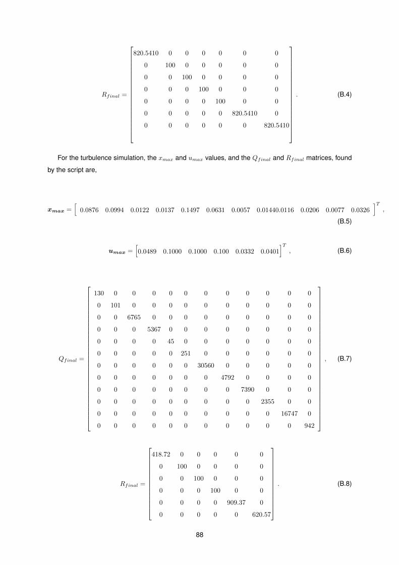
Rfinal =

820.5410 0 0 0 0 0 0

0 100 0 0 0 0 0

0 0 100 0 0 0 0

0 0 0 100 0 0 0

0 0 0 0 100 0 0

0 0 0 0 0 820.5410 0

0 0 0 0 0 0 820.5410

. (B.4)

For the turbulence simulation, the xmax and umax values, and the Qfinal and Rfinal matrices, found

by the script are,

xmax =[

0.0876 0.0994 0.0122 0.0137 0.1497 0.0631 0.0057 0.01440.0116 0.0206 0.0077 0.0326]T

,

(B.5)

umax =[0.0489 0.1000 0.1000 0.100 0.0332 0.0401

]T, (B.6)

Qfinal =

130 0 0 0 0 0 0 0 0 0 0 0

0 101 0 0 0 0 0 0 0 0 0 0

0 0 6765 0 0 0 0 0 0 0 0 0

0 0 0 5367 0 0 0 0 0 0 0 0

0 0 0 0 45 0 0 0 0 0 0 0

0 0 0 0 0 251 0 0 0 0 0 0

0 0 0 0 0 0 30560 0 0 0 0 0

0 0 0 0 0 0 0 4792 0 0 0 0

0 0 0 0 0 0 0 0 7390 0 0 0

0 0 0 0 0 0 0 0 0 2355 0 0

0 0 0 0 0 0 0 0 0 0 16747 0

0 0 0 0 0 0 0 0 0 0 0 942

, (B.7)

Rfinal =

418.72 0 0 0 0 0

0 100 0 0 0 0

0 0 100 0 0 0

0 0 0 100 0 0

0 0 0 0 909.37 0

0 0 0 0 0 620.57

. (B.8)

88

B.2 LQR Gain Matrix

The engine failure gain matrix associated with the value the script found (ρ = 10) utilizing the matrices

(B.2) and (B.2) is,

KLQR =

0.4015 −0.2383 −6.4192 −22.2477 0.0664 −1.6801 0.0313 0.0104 0.0220 0.0243 0.0559 0.0023

0 0 0 0 0 0 0 0 0 0 0 0

0 0 0 0 0 0 0 0 0 0 0 0

2.2125 −0.1379 −2.7448 −15.1224 0.4291 1.9008 0.7640 −0.1407 −0.1431 −0.1801 −1.0060 −0.1232

−0.7070 0.1320 2.5032 9.7677 −0.1128 −0.7113 1.5885 −0.4390 −0.6906 −0.6607 −3.1044 −0.3490

−0.1092 0.0008 −0.0394 1.8940 −0.0181 −0.0582 0.1099 −0.0700 −0.0246 −0.0788 −0.2115 −0.0221

−0.2127 0.0010 −0.0658 3.1405 −0.0392 −0.0330 0.0501 −0.0192 −0.0365 −0.0370 −0.2408 −0.0278

,

(B.9)

The control penalty parameter for which the script first found level one flying qualities, in the turbu-

lence simulation, was for ρ = 20. The computed gain matrix for this case is, taking in account matrices

(B.7) and (B.8),

KLQR =

0.1311 −0.0311 −1.1820 −1.9993 0.0578 −0.1048 0 0 0 0 0 0

0.1704 0.0059 −0.3148 −0.1317 0.0644 0.1929 −0.4609 0.0833 1.3167 0.2392 1.1593 0.1684

0.0078 0.1384 2.3626 −0.0199 0.0070 0.0723 0 0 0 0 0 0

0.1704 0.0059 −0.3148 −0.1317 0.0644 0.1929 0.4609 −0.0833 −1.3167 −0.2392 −1.1593 −0.1684

0 0 0 0 0 0 −0.4194 −0.5271 −0.0144 −0.8739 −1.5349 −0.2092

0 0 0 0 0 0 0.0069 −0.0527 −0.1918 −0.1024 −0.3518 −0.0516

.

(B.10)

89

flight dynamics and simulation of a generic aircraft for ... · este simulador de voo permite...

Documents