Flight Dynamics and Control Lecture 5:

Solution of the Equations of Motion

G. Dimitriadis University of Liege

Solution of the Equations of Motion

•  We have seen that the equations of motion of a rigid aircraft can be of the form:

•  This is state space form, , where x are the system states and u are the system inputs

!v!p!r!ϕ!ψ

#

$

%%%%%%

&

'

((((((

=

−0.0565 29.072 −175.610 9.6783 1.6022−0.0601 −0.7979 0.2996 0 0

9.218 ×10−3 −0.0179 −0.1339 0 00 1 0 0 00 0 1 0 0

#

$

%%%%%%

&

'

((((((

vprϕ

ψ

#

$

%%%%%%

&

'

((((((

+

−0.2678 2.00924.6982 0.77030.0887 −1.35750 00 0

#

$

%%%%%%

&

'

((((((

ξ

ς#

$%&

'(

!x = Ax + Bu

x = [ v p r ϕ ψ ]T , u = [ ξ ς ]T

How to solve

•  The equations can be re-written in the form

•  And pre-multiplied by yielding

•  The left-hand side of these equations is in fact , so that

!x − Ax = Bu

e−At

e−At !x − e−AtAx = e−AtBu

ddt

e−Atx( )ddt

e−Atx( ) = e−AtBu

General Solution

•  In this form, the state space equations are ‘variables separable’ so that they can be easily integrated as

•  So that

•  And, finally,

d e−Atx( )0

t

∫ = e−AτBu τ( )dτ0

t

∫

e−Atx t( ) − e−A0x 0( ) = e−AτBu τ( )dτ0

t

∫ or e−Atx t( ) = x 0( ) + e−AτBu τ( )dτ0

t

∫

x t( ) = eAtx 0( ) + eA t−τ( )Bu τ( )dτ0

t

∫

Evaluating the general solution

•  The evaluation of the general solution is not trivial. There are two major difficulties: – The matrix exponential – The input function integral

•  The matrix exponential is usually called the ‘state transition matrix’

•  First we will discuss some properties of matrix exponentials

eAt

eA t−τ( )Bu τ( )dτ0

t

∫

Matrix exponentials •  A matrix exponential is not equal to the

exponential of all the elements of the matrix. •  If , then

•  However, if , i.e. it is diagonal, then

•  In general, the matrix exponential can be calculated either using an eigensolution or a series approximation

E =1 23 4!

"#$

%&eE ≠

e1 e2

e3 e4"

#$%

&'

E =1 00 4!

"#$

%&

eE =e1 00 e4

!

"#$

%&

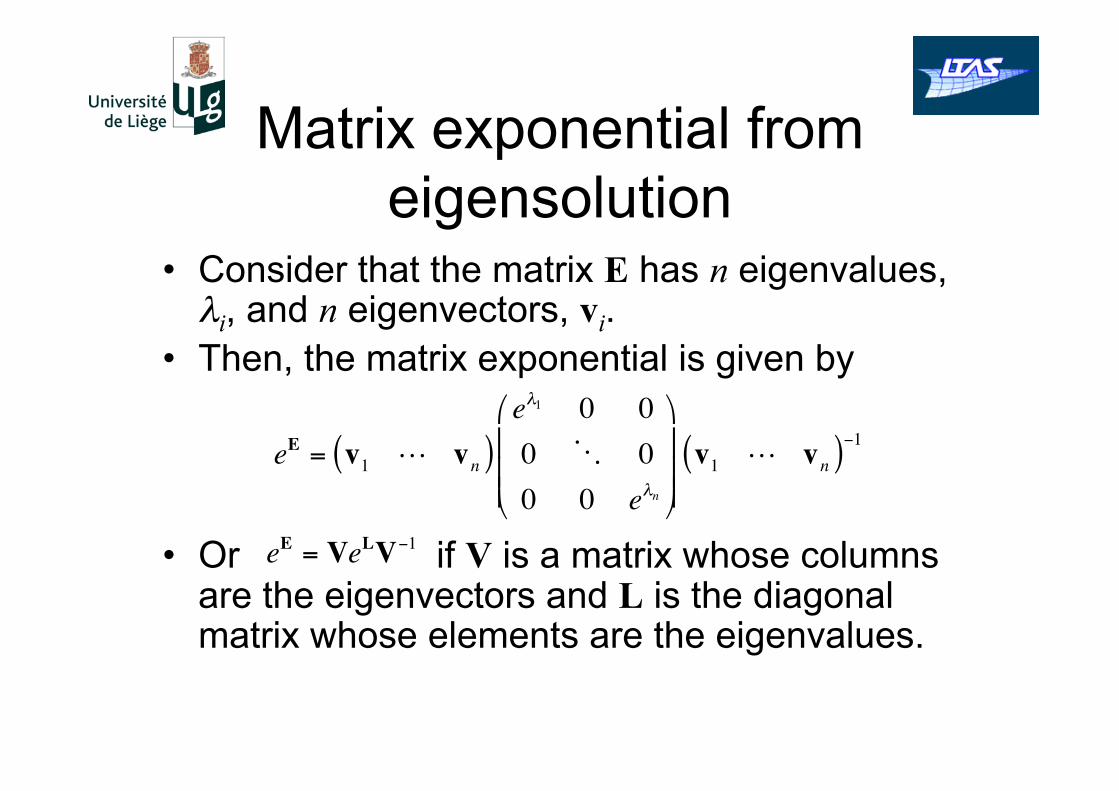
Matrix exponential from eigensolution

•  Consider that the matrix E has n eigenvalues, λi, and n eigenvectors, vi.

•  Then, the matrix exponential is given by

•  Or if V is a matrix whose columns are the eigenvectors and L is the diagonal matrix whose elements are the eigenvalues.

eE = v1 ! vn( )eλ1 0 00 " 00 0 eλn

"

#

$$$

%

&

'''v1 ! vn( )−1

eE = VeLV−1

Example

•  Consider the state space system

•  Let

•  Calculate the state transition matrix

!x =

0 1−1 0"

#$%

&'x

A =0 1−1 0#

$ %

&

' (

eAt

Solution •  The eigenvalues of A are i and -i and

the eigenvectors are

•  The eigenvalues of At are it and -it and the eigenvectors are those of A.

•  Then,

•  or

V =1 1i −i"

#$%

&'

eAt =1 1i −i"

#$%

&'eit 00 e− it

"

#$%

&'1 1i −i"

#$%

&'

−1

=1 1i −i"

#$%

&'eit 00 e− it

"

#$%

&'1 / 2 −i / 21 / 2 i / 2"

#$%

&'

eAt =cos t sin t− sin t cos t"

#$%

&'

Series form

•  In cases where the input is zero, i.e. u(t)=0, the expression for the solution of the state space equations can be written in a series form as:

•  or

•  Where ci is the ith element of vector c=V-1x(0).

x t( ) = v ieλi tci

i=1

n

∑

x t( ) = VeLtV−1x 0( ) = VeLtc

Input Integral •  The form of the input integral depends on the

form of the function u(t). There can be no general expression for it

•  As was done with the unforced solution, the expression for the integral can be written in series form in the following way:

•  Or

•  Where di(τ) is the ith element of vector d=V-1Bu(τ)

eA t−τ( )Bu τ( )dτ0

t

∫ = v ieλi t−τ( )di τ( )dτ

0

t

∫i=1

n

∑

eA t−τ( )Bu τ( )dτ0

t

∫ = VeL t−τ( )V−1Bu τ( )dτ0

t

∫ = VeL t−τ( )d τ( )dτ0

t

∫

Full response

•  Therefore, the full response of the aircraft can be written in series form as

•  where ci is the ith element of c=V-1x(0) and di(τ) is the ith element of d=V-1Bu(τ).

•  Of course u(t) must be selected in order to calculate the full response.

•  The usual choices are elementary input functions: step, ramp, impulse

x t( ) = vii=1

n

∑ eλ i tci + vieλ i t−τ( )di

0

t

∫ τ( )dτi=1

n

∑

Step response

•  If the input signal is a constant u(t)=u(0) and x(0)=0 then the response of the system is called the ‘step response’.

•  The input integral becomes

•  So that the full solution is

eA t−τ( )Bu τ( )dτ0

t

∫ = v ieλi t−τ( )di 0( )dτ

0

t

∫i=1

n

∑

= v idi 0( )−λii=1

n

∑ eλi t−τ( )τ =0

τ = t= − v i

di 0( )λii=1

n

∑ 1− eλi t( )

x = − v idi 0( )λii=1

n

∑ 1− eλi t( )

Step response of F4 longitudinal equations

The response is 0 at t=0. A short period (high frequency) response is damped out quickly, followed by a long period (low frequency) response that lasts 10 minutes

Step response of F4 lateral equations

The response is 0 at t=0. There is no long period response, only a short period (high frequency) response that lasts under 1 minute

Ramp Response •  If the input increases linearly from zero

and x(0)=0 the system’s response is called the ramp response.

•  Write the input as u=mt. •  The input integral becomes

•  Where d=V-1Bm, so that

eA t−τ( )Bu τ( )dτ0

t

∫ = v ieλi t−τ( )diτdτ0

t

∫i=1

n

∑

= v idiλi2

i=1

n

∑ −λiτ −1( )eλi t−τ( )( )τ =0

τ = t= − v i

diλi2

i=1

n

∑ 1+ λit − eλi t( )

x = − v idiλi2

i=1

n

∑ 1+ λit − eλi t( )

What exactly is a ramp? •  Step inputs can result

in unwanted short period oscillations.

•  A ramp input can have the same effect as a step input but this effect is achieved gradually (over t0 seconds)

t

u

t0

Ramp Step

Important point about ramp response

•  A ramp response that keeps rising makes no sense.

•  A ramp response is usually followed by a step

•  The force input is of the form

•  The solution of the equations of motion must be evaluated in these intervals

u =mt if t ≤ t0mt0 if t > t0"#$

Solution to ramp followed by step

•  The solution is of the form

•  Where, in this case, c=V-1x(t0) and d=V-1Bm.

x =− vi

diλi

2i=1

n

∑ 1+λit − eλit( ) if t ≤ t0

vieλi t−t0( )ci

i=1

n

∑ − vidit0λii=1

n

∑ 1− eλi t−t0( )( ) if t > t0

⎧

⎨

⎪⎪

⎩

⎪⎪

Ramp response of F4 longitudinal equations

The response is 0 at t=0. This time there is no short period oscillation, just a gentle increase up to t0=20s. The long period oscillation is as long as before but the amplitude is slightly smaller.

Ramp response of F4 lateral equations

The response is 0 at t=0. The short period response is replaced by a gentle almost linear rise. When the short period response does occur, it has a very low amplitude.

Impulse Response

•  An impulse response is usually defined as the response of a system to the Dirac delta function, δ(t).

•  The Dirac delta is defined as:

•  And has the properties that:

δ t( ) =∞ if t = 00 if t ≠ 0

$%&

δ t( )dt−∞

∞

∫ = 1 and f t( )δ t( )dt−∞

∞

∫ = f 0( )

Solution to impulsive input •  The initial conditions are still zero, i.e. x(0)=0

•  The input is of the form u=mδ(t). •  The input integral becomes:

•  Where d=V-1Bm and m=[1 0]T or m=[0 1]T . •  Impulse responses should only be applied

to one input at a time.

eA t−τ( )Bu τ( )dτ0

t

∫ = v ieλi t−τ( )diδ τ( )dτ

0

t

∫i=1

n

∑

= v idii=1

n

∑ eλi t

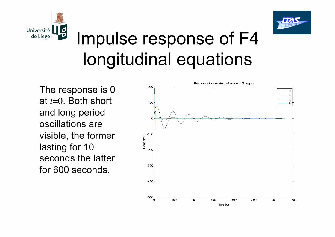
Impulse response of F4 longitudinal equations

The response is 0 at t=0. Both short and long period oscillations are visible, the former lasting for 10 seconds the latter for 600 seconds.

Impulse response of F4 lateral equations

The response is 0 at t=0. A short period vibratory response dies away after 50 seconds. A non-vibratory response flattens out (at a non-zero steady state) after 300 seconds.

Modes of vibration

•  The longitudinal and lateral results demonstrate several modes of vibration: –  Longitudinal modes:

•  Short Period Oscillation •  Phugoid

–  Lateral modes: •  Spiral mode •  Roll subsidence •  Dutch roll

Phugoid oscillations

•  Notice that the application of ramp input only removed the short period oscillations and did not affect the long period ones.

•  These oscillations are termed phugoids and they occur only in the longitudinal direction.

•  Phugoid periods: –  Microlight aircraft: 15-25s –  Light aircraft: over 30s –  Jet aircraft: minutes

•  Phugoids are neutralized by re-trimming the aircraft in the new flight condition.

Phugoid Videos

Cause of Phugoids •  Phugoids are direct results of elevator

deflection around a trimmed position. •  The resulting pitch change will cause the

aircraft to tip either nose up or nose down. •  If it tips nose down it will gain speed,

therefore lift and tip nose up again. •  If it tips nose up it will loose speed, therefore

lift and tip nose down. •  The angle of attack does not change - the

aircraft remains tangent to the flight path. •  The oscillation has very low damping and can

last for a long time

Phugoid mode approximation

•  Lanchester model: – Aircraft initially in steady flight – Total energy of aircraft remains the same – The incidence is constant – The thrust balances the drag – The motion is slow so that pitch rate effects

can be ignored

Lanchester model

12mV0

2 =12mV 2 + mgh = const.Energy conservation:

So that: V2=V0

2-2gh

Lift coefficient conservation: L=mg-ρghSCL

Lanchester model (2)

•  Therefore, the total force in the horizontal direction is given by:

•  Substituting from the lift equation yields:

•  The frequency of the phugoid is then

m˙ ̇ h = Lcosθ − mg ≈ L − mg

m˙ ̇ h + ρgSCL

m# $

% &

h = 0

ω p =ρgSCL

m=g 2V0

Better approximation

•  A better approximation can be obtained from the longitudinal equations of motion.

•  Only the equations for u and θ are retained, along with the conditions

•  Then ,

˙ w = ˙ q = 0

ζ pω p =gCD

CLV0

, ω p =g 2V0

More about Phugoids •  Phugoid period

increases with airspeed. Phugoid damping increases with airspeed.

•  Compressibility effects •  Period and damping

for a Boeing 747 at several altitudes and Mach numbers

Nhalf= number of periods until the amplitude is halved

Effect of static stability margin

Small static margins decrease the period and decrease the damping of Phugoids. The choice of static margin must be balanced also with the desired degree of static stability

Short period oscillations

•  Short period oscillations are driven by the angle of attack (in french they are called oscillations d’incidence).

•  Speed changes are negligible, u=0. •  It is essentially a 2-DOF mechanism

involving w and q. •  They occur after abrupt input changes.

Slower input changes do not cause significant short period oscillations

Short period approximation •  The longitudinal equations of motion

during a short period oscillation can be simplified to:

•  Where zw, mw etc are constants. •  We can further simplify by assuming that

changes in θ do not affect the derivatives in q and w:

˙ w ˙ q ˙ θ

#

$

% % %

&

'

( ( (

=

zw zq zθmw mq mθ

0 1 0

#

$

% % %

&

'

( ( (

wqθ

#

$

% % %

&

'

( ( (

+

zηmη

0

#

$

% % %

&

'

( ( (

η

˙ w ˙ q

"

# $ %

& ' =

zw zq

mw mq

"

# $

%

& '

wq"

# $ %

& ' +

zηmη

"

# $

%

& ' η

Short period approximation

•  Substituting from the longitudinal equations of motion yields:

•  If was assume:

˙ w ˙ q

"

# $ %

& ' =

˜ Z wm − ˜ Z ˙ w

˜ Z q + mUe

m − ˜ Z ˙ w ˜ M wIy

˜ M qIy

"

#

$ $ $ $

%

&

' ' ' '

wq"

# $ %

& ' +

˜ Z ηm − ˜ Z ˙ w

˜ M ηIy

"

#

$ $ $ $

%

&

' ' ' '

η

˜ Z q << mUe and ˜ Z ˙ w << m

˙ w ˙ q

"

# $ %

& ' =

˜ Z wm

Ue

˜ M wIy

˜ M qIy

"

#

$ $ $ $

%

&

' ' ' '

wq"

# $ %

& ' +

˜ Z ηm˜ M ηIy

"

#

$ $ $ $

%

&

' ' ' '

η

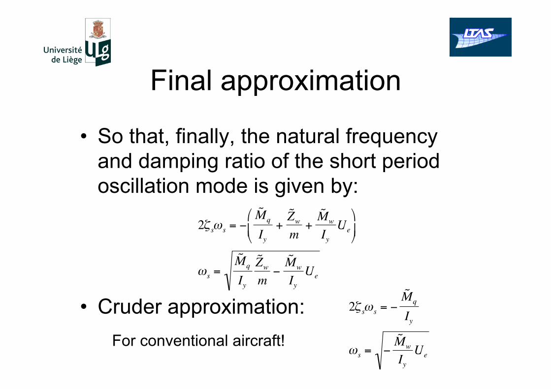
Final approximation

•  So that, finally, the natural frequency and damping ratio of the short period oscillation mode is given by:

•  Cruder approximation:

2ζ sωs = −˜ M qIy

+˜ Z wm

+˜ M wIy

Ue

%

& '

(

) *

ωs =˜ M qIy

˜ Z wm−

˜ M wIy

Ue

2ζ sωs = −˜ M qIy

ωs = −˜ M wIy

UeFor conventional aircraft!

Short Period Dependencies •  The period generally

decreases with airspeed. The damping can either decrease or increase

•  Compressibility effects •  Period and damping

for a Boeing 747 at several altitudes and Mach numbers

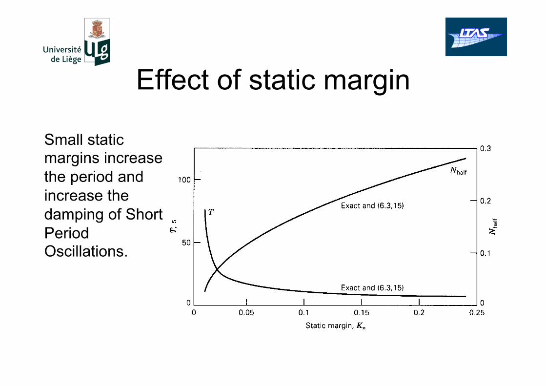
Effect of static margin

Small static margins increase the period and increase the damping of Short Period Oscillations.

Spiral mode •  This mode is quite visible in the impulse

response of the lateral equations •  It is the non-oscillatory mode with large time

constant •  It is mainly a yaw movement with a little roll •  This mode can be stable or unstable. It is

unstable quite often but that is not a problem because of its large time constant

•  The typical half-life of a spiral mode is of the order of a minute.

•  The spiral movement is usually stopped by a corrective control input

Spiral Mode Video

Roll subsidence

•  An impulsive aileron input will start the aircraft rolling.

•  In general, the aircraft will stop rolling with time (i.e. the roll rate becomes zero after sufficient time)

•  The aircraft will find itself at a roll angle which depends on how fast the roll rate tends to zero.

•  This phenomenon is called roll subsidence.

Roll Subsidence Video

Dutch Roll •  The name Dutch Roll is due to the fact that

the phenomenon resembles an ice skating figure called Dutch Roll.

•  The centre of gravity remains on a straight trajectory while the roll and yaw angles oscillate.

•  The roll velocity also oscillates but the yaw velocity is very low.

•  The Dutch roll damping increases with airspeed while its period first increases and then decreases with airspeed.

•  The typical period of a Dutch roll is in the order of 5 to 10 seconds.

Dutch Roll graphic Imagine all drawings on a single straight line

Dutch Roll Videos

Dutch Roll approximation •  There is little consensus on how to simplify the Dutch Roll

mode. •  In fact there is little consensus on what the Dutch Roll

mode involves for a generic airplane. •  Cook states that ‘it is probably true for most airplanes that

the roll to yaw ratio is less than one’. –  ‘… in some cases (it) may be much less than one’. –  Using this assumption, a simplification of the equations of

motion can be carried out. •  McCormick states that the roll and yaw motions have

approximately the same magnitude. He backs it up with results from the Piper Cherokee aircraft. –  He states that the Dutch Roll motion is characterized by roll,

yaw and sideslip. –  In this case, no real simplification can be carried out.

Cook’s Dutch Roll approximation

•  Use the longitudinal equations of motion with the assumptions:

•  So that,

•  and

˙ p = p = ˙ φ = φ = 0

˙ v ˙ r "

# $ %

& ' =

˜ Y vm

V0

˜ N vIz

˜ N rIz

"

#

$ $ $ $

%

&

' ' ' '

vr"

# $ %

& '

2ζ dωd = −˜ N rIz

+˜ Y vm

%

& '

(

) *

ωs =˜ N rIz

˜ Y vm−

˜ N vIz

V0

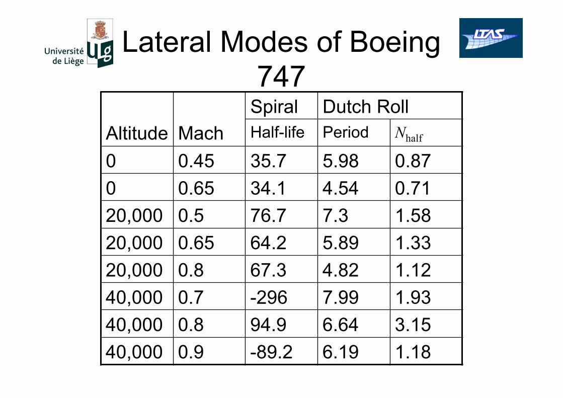
Lateral Modes of Boeing 747

Altitude

Mach

Spiral Dutch Roll Half-life Period Nhalf

0 0.45 35.7 5.98 0.87 0 0.65 34.1 4.54 0.71 20,000 0.5 76.7 7.3 1.58 20,000 0.65 64.2 5.89 1.33 20,000 0.8 67.3 4.82 1.12 40,000 0.7 -296 7.99 1.93 40,000 0.8 94.9 6.64 3.15 40,000 0.9 -89.2 6.19 1.18

Stability Analysis

•  The stability of the equations of motion is analysed as usual

•  The stability depends on the eigenvalues of the matrix A

•  If all of the eigenvalues have negative real parts the system is stable

•  If at least one eigenvalues has a positive real part the system is unstable

•  If at least one of the eigenvalues has a zero real part the system is neutrally stable

Lateral Equations stability •  The lateral equations are usually almost

neutrally stable. •  Example: F4 lateral equations have these

eigenvalues: -0.1602 + 1.8141i, -0.1602 - 1.8141i, -0.6506, -0.0172, -0.000.

•  The -0.000 eigenvalue is due to the fact that aircraft have little or no restoring force in the roll direction.

•  Fighter aircraft, like the F4, are designed to have no restoring force in roll and some aircraft, like the F104, were designed to be unstable in roll.