flexible structure impact modeling with a particle method - nathan donald obringer

ABSTRACT

OBRINGER, NATHAN DONALD. Flexible Structure Impact Modeling With a Particle Method. (Under the direction of Jeffrey W. Eischen).

The purpose of this research was to develop the capability to handle flexible structure

impact problems using the particle method. A MATLAB computer code that implemented

the particle-based formulation capable of handling stretch and bend forces, external forces,

and contact was created and thoroughly tested. The computer code was validated where

possible using classical beam and plate theories. After developing a MATLAB computer

code particle model, the particle model is to be embedded in the computational fluid dynamic

code produced at North Carolina State University termed, the Room Simulator. In order to

do so, the particle model had to be capable of reading and writing STL (stereo-lithography)

files to use as input and output. The particle model is three-dimensional and can handle

internal and external forces. Internal forces include in-plane membrane forces, out-of-plane

bending forces, and absolute damping forces. External forces include all external applied

loads, gravitational forces, and effective forces due to pressure. The MATLAB computer

code was equipped with a contact detection and update algorithm with a point-to-plane

collision detection and a velocity update scheme. In order to produce simulations involving

actual materials, the procedure to measure actual material properties has been documented.

Also, the procedure to convert from experimentally determined fabric mechanical properties

to effective stiffness values useful in the MATLAB computer code is described. Seven

simulations were used to demonstrate the utility of the MATLAB computer code.

Flexible Structure Impact Modeling With a Particle Method

by Nathan Donald Obringer

A thesis submitted to the Graduate Faculty of North Carolina State University

in partial fulfillment of the requirements for the degree of

Master of Science

Mechanical Engineering

Raleigh, North Carolina

2010

APPROVED BY:

_______________________________ ______________________________ Dr. Jack R. Edwards Dr. Arkady Kheyfets

________________________________ Dr. Jeffrey W. Eischen

Committee Chair

ii

DEDICATION

To my parents, Tim and Patty Obringer.

You have loved and cared for me,

And you have been there from day one.

I hope you cherish all the memories

And are proud of the man I have become!

To my brother, Adam Obringer.

As you have begun to mature into a fine young man,

The bond we share has grown tighter than ever before!

Thank you for the support!

To the one and only, Lauren Boris.

I am glad you found me on that summer day.

While times have been tough being apart from you,

I hope this brings a smile to your face

And signifies a new chapter in the book we write together!

You deserve more credit than I can offer,

But let me just say thank you for being there when times were rough

And I needed you more than you knew!

iii

BIOGRAPHY

Nathan Obringer was born in September 1985 in Pittsburgh, Pennsylvania to Tim and Patty

Obringer. Five years later, in August 1990, his brother Adam became a part of his life!

Nathan attended school in the Baldwin-Whitehall School District before graduating from

Baldwin High School in 2003. Nathan went on to pursue his Bachelor’s Degree in

Mechanical Engineering at Penn State University. After obtaining his degree from Penn

State University in May 2008, he enrolled at North Carolina State University where he

pursued his Master’s Degree in Mechanical Engineering. His time in North Carolina

concluded with the successful defense of his thesis on June 4, 2010. Nathan is returning to

Pittsburgh to continue to explore life’s many challenges while using his skills and knowledge

to contribute to a world which has given him so much!

iv

ACKNOWLEDGMENTS

This thesis would not have been possible had it not been for the guidance and support of a

few very important people. I express my sincere gratitude to:

Dr. Jeffrey W. Eischen, who stuck with me when times were tough, and through your

help and support, we were able to make huge strides, culminating with the completion

of my part of this project. I appreciate all of your help and the knowledge I have

gained under your guidance.

Dr. Jung-Il Choi, you were the one I turned to when I had programming questions.

Thank you for your help, suggestions, and for the contributions you made to this

project.

I would like to thank Dr. Jack Edwards and Dr. Arkady Kheyfets for serving on my

research committee.

I would like to thank the Naval Surface Warfare Center for providing the grant which

made this research possible.

To my family, you were there for me and offered me encouragement when I was

down; you reminded me that this would be an accomplishment I would cherish for the

rest of my life!

Laur, you were my rock when I needed support and you always knew what to do or

what to say to brighten my day; I appreciate you putting up with me and listening to

me describe my project to you day-in and day-out; you are the best!

v

TABLE OF CONTENTS LIST OF TABLES ............................................................................................................... viii

LIST OF FIGURES ............................................................................................................... ix

1 Introduction ..................................................................................................................... 1

1.1 Background and Objective of Research ................................................................. 1

1.2 Literature Review ..................................................................................................... 3

2 Particle Method Formulation ......................................................................................... 9

2.1 One-Dimensional Formulation................................................................................ 9

2.1.1 One-Dimensional Stretch Formulation ........................................................... 9

2.1.2 One-Dimensional Bend Formulation ............................................................ 14

2.1.3 Damping Force ................................................................................................ 18

2.1.4 One-Dimensional Equation of Motion .......................................................... 19

2.1.5 One-Dimensional Validation with Beam Theory ......................................... 19

2.2 Three-Dimensional Formulation .......................................................................... 26

2.2.1 Three-Dimensional Stretch Formulation ...................................................... 26

2.2.2 Three-Dimensional Bend Formulation ......................................................... 28

2.2.3 Boundary Conditions ...................................................................................... 35

2.2.4 Initially Curved Surfaces ............................................................................... 36

2.2.5 Gravitational Forces ....................................................................................... 36

2.2.6 Effective Force due to Pressure ..................................................................... 36

2.2.7 Damping Force ................................................................................................ 37

2.2.8 Equations of Motion ....................................................................................... 38

2.2.9 Three-Dimensional Validation with Plate Theory ....................................... 38

3 Contact Formulation ..................................................................................................... 51

3.1 Contact Detection ................................................................................................... 51

3.2 Contact Update ....................................................................................................... 65

vi

3.3 Contact Algorithm: Efficiency Improvement Methods ...................................... 69

4 Fabric Material Properties ........................................................................................... 72

4.1 Cantilever Bending Test ........................................................................................ 72

4.2 Obtaining the k0 Stiffness Coefficient ................................................................... 76

4.3 Example: Canvas Tent Material ........................................................................... 77

4.4 Obtaining the Bending Stiffness Coefficient kb.................................................... 78

5 Results ............................................................................................................................. 83

5.1 Case 1: Single Impactor Triangle ......................................................................... 84

5.2 Case 2: Multiple Impacts ....................................................................................... 91

5.3 Case 3: Glancing Blow ........................................................................................... 95

5.4 Case 4: Sphere Passing through a Plate with a Slit ............................................. 99

5.5 Case 5: Soldier Moving into Full Tent, No Pressure ......................................... 104

5.5.1 Comparing Particle Model Results with LS-DYNA .................................. 109

5.6 Case 6: Soldier Moving into Full Tent, with Pressure ...................................... 116

5.7 Case 7: Soldier on a Gurney ................................................................................ 119

6 Conclusions and Recommendations .......................................................................... 124

6.1 Conclusions ........................................................................................................... 124

6.2 Recommendations for Future Research ............................................................. 125

REFERENCES .................................................................................................................... 126

APPENDIX .......................................................................................................................... 128

A Equations of Motion Matlab Function Code ......................................................... 129

B Runge-Kutta Matlab Function Code ..................................................................... 136

C 11 x 11 Mesh Input File ........................................................................................... 137

D Cantilever Bending Test Spreadsheet Results ....................................................... 157

E Case 1 Main Matlab Code ....................................................................................... 158

F Case 2 Main Matlab Code (Input Parameters Only) ........................................... 172

vii

G Case 2 Multiple Impactor Sample Input File ........................................................ 173

H Case 3 Main Matlab Code (Input Parameters Only) ........................................... 174

I Case 4 Main Matlab Code (Input Parameters Only) ........................................... 175

J Case 5 Main Matlab Code (Input Parameters Only) ........................................... 176

K Case 6 Main Matlab Code (Input Parameters Only) ........................................... 177

L Case 7 Main Matlab Code (Input Parameters Only) ........................................... 178

viii

LIST OF TABLES

Table 2.1. Particle Model Stiffness Coefficient Values ...................................................... 20 Table 2.2. Comparison Results: Large Deflection Theory vs. 40 Particle Model ........... 24 Table 2.3: Square Plate, Deflection Results, Comparing Particle Model with Plate

Theory .................................................................................................................. 41 Table 3.1. Contact Algorithm Variables ............................................................................. 61 Table 4.1. Measured Properties ........................................................................................... 77 Table 4.2. Calculated Properties .......................................................................................... 78 Table 4.3. Data for kb vs. P .................................................................................................. 81

ix

LIST OF FIGURES

Figure 2.1. Stretching Elements ........................................................................................... 10 Figure 2.2. Single Spring Model of a Bar ............................................................................ 11 Figure 2.3. Multiple Spring Model of a Bar ....................................................................... 12 Figure 2.4. Fixed Displacement Boundary Condition for Particle 1 ................................ 13 Figure 2.5. Free Edge Boundary Condition for Particle n ................................................ 13 Figure 2.6. Bending Stiffness Element ................................................................................ 15 Figure 2.7. Fixed Displacement Boundary Condition for Particle 1 ................................ 17 Figure 2.8. Free Edge Boundary Condition for Particle n ................................................ 18 Figure 2.9. Standard Small Deflection Beam Theory Parameters ................................... 19 Figure 2.10. Bending Model vs. Small Deflection Beam Theory ...................................... 21 Figure 2.11. Large Deflection Beam Theory Parameters .................................................. 22 Figure 2.12. PL2/EI vs. δv/L .................................................................................................. 24 Figure 2.13. PL2/EI vs. δh/L .................................................................................................. 25 Figure 2.14. 3D Stretching Elements ................................................................................... 27 Figure 2.15. Triangular Mesh with Emphasis on Two Elements Sharing Common

Edge ................................................................................................................... 28 Figure 2.16. 3D Triangular Mesh- Undeformed and Deformed Elements ...................... 29 Figure 2.17. Applied Uniform Pressure on Element 1-2-4 ................................................ 37 Figure 2.18. Flexible Structure: Triangular Mesh ............................................................. 39 Figure 2.19. Simply Supported on all Four Sides, Center Point Load ............................. 40 Figure 2.20. δz/Lx vs. x: Particle Model Compared with First 11 Terms of Plate

Theory (for y = 0.5) .......................................................................................... 42 Figure 2.21. δz/Lx vs. kb, Point Load, 4 Simply Supported Edges, Center Particle ......... 43 Figure 2.22. Simply Supported on Two Edges with a Center Point Load ....................... 44 Figure 2.23. Simply Supported on Two Edges with a Line Load ..................................... 46 Figure 2.24. Simply Supported on all Four Edges with a Center Point Load ................. 47 Figure 2.25. Simply Supported on all Four Edges with a Line Load ............................... 49 Figure 3.1. Defining the Ultimate Goal of the Contact Algorithm ................................... 52 Figure 3.2. Possible Contact Situations ............................................................................... 53 Figure 3.3. Plane ijk .............................................................................................................. 54 Figure 3.4. Closest Projection of Point P onto the Plane ................................................... 56 Figure 3.5. Before and After Configurations used to Define Contact .............................. 57 Figure 3.6. Point Q Projected Inside Element i-j-k ............................................................ 58 Figure 3.7. Point Q Lying Outside Triangle ijk .................................................................. 59 Figure 3.8. Multiple Contact Detections for Element i-j-k ................................................ 63

x

Figure 3.9. Current and Predicted Impactor and Structural Element Vertex Positions .............................................................................................................. 66

Figure 3.10. Velocity Update Applied at Contact Vertices ............................................... 68 Figure 3.11. Front View of the Distance Check Method ................................................... 70 Figure 3.12. Front-View of the Box Method ....................................................................... 71 Figure 4.1. Cantilever Bending Test Apparatus ................................................................ 73 Figure 4.2. Overhang Length of the Fabric ........................................................................ 74 Figure 4.3. Simply Supported Rectangular Plate Used for the Tuning Approach ......... 79 Figure 4.4. Particle Mesh Used for Bending Stiffness Tuning .......................................... 80 Figure 4.5. kb vs. P ................................................................................................................. 82 Figure 5.1. Case 1 Initial Flexible Structure and Impactor Configuration ..................... 85 Figure 5.2. Forces and Velocity versus Time Plot .............................................................. 86 Figure 5.3. Single Impactor Triangle Animation Sequence .............................................. 88 Figure 5.4. Time-History Plot for Structural Element Vertex 276 ................................... 89 Figure 5.5. Time-History Maximum Penetration .............................................................. 90 Figure 5.6. Case 2 Initial Flexible Structure and Impactor Configuration ..................... 92 Figure 5.7. Multiple Impacts with Flexible Structure Animation Sequence ................... 94 Figure 5.8. Case 3 Initial Flexible Structure and Impactor Configuration ..................... 96 Figure 5.9. Single Impactor Triangle, Glancing Blow Animation Sequence ................... 98 Figure 5.10. Case 4 Initial Flexible Structure and Sphere Configuration ..................... 100 Figure 5.11. Forces and Velocity versus Time Plot .......................................................... 101 Figure 5.12. Sphere Through Plate Slit Animation Sequence ........................................ 103 Figure 5.13. Initial Configuration of Soldier and Full Hexagonal-shaped Tent ........... 105 Figure 5.14. Pan View of Initial Soldier and Tent Configuration .................................. 106 Figure 5.15. Single Soldier Entering Full Hexagonal-Shaped Tent Animation

Sequence.......................................................................................................... 108 Figure 5.16. Location of Vertex 1872 ................................................................................ 110 Figure 5.17. Particle Model Comparison with LS-DYNA Vertex 1872 ......................... 111 Figure 5.18. Comparison Between Particle Model and LS-DYNA Animation

Sequence.......................................................................................................... 112 Figure 5.19. Single Soldier Entering Full Tent with Pressure Animation Sequence .... 118 Figure 5.20. Soldier on Gurney Entering Full Tent Animation Sequence .................... 121 Figure 5.21. Time-History Plot for Structural Element Vertex 1872 ............................. 122 Figure 5.22. Time-History Plot of the Maximum Penetration ........................................ 123

1

1 Introduction

1.1 Background and Objective of Research

The long term goal of this research project was to produce computational simulations of

human ingress/egress events into flexible structures located in chemically contaminated

areas, while tracking the concentration of toxic species during such events. In a chemically

contaminated environment, it is known that certain gas species may be transported from one

location to another via human motion. This transportation can cause the infiltration of a

previously safe environment with harmful pollutants. In an attempt to understand how this

transportation occurs, the immediate goal of this research project was to create a structural

particle-based computer code capable of producing realistic results aimed at studying the

deformation of flexible structures accounting for contact with models of moving humans.

Through recent work, Dr. Jack Edwards’s research group at North Carolina State University

has developed a Room Simulator computational fluid dynamics (CFD) code. The Room

Simulator solves the time-dependent, incompressible Navier-Stokes equations, expanded to

include gas-phase heat conduction and gas-phase agent transport. The Room Simulator

combines large-eddy simulation techniques for turbulent wake resolution with immersed-

boundary methods to account for the effects of moving features. This approach embeds a

surface mesh consisting of structured or unstructured elements within a flow. The surface

meshes may be closed or of zero-thickness and can consist of multiple parts which can be

separately animated. The framework of the Room Simulator is highly suited for a detailed

examination of ingress/egress events into flexible structures. A long-term goal is for Room

2

Simulator to be updated to incorporate pre-programmed, mission-specific human activity and

to link with existing urban airflow models that will provide external environmental

conditions. Also, there is a need to add a particle model for fabric structural response to

enable realistic simulations of flexible or semi-rigid entryways. The contribution of this

research project stems from this need to add a particle model.

The response of a flexible structure is crucial when studying ingress/egress events.

Depending on the type of door, entry/exit into these structures can cause deformation of a

flexible or semi-rigid fabric structure. The door opening/closing event itself can cause

separation and reconstitution of fabric panels and fabric deformation can occur due to impact

loads. The effects of gravity and pressure can also cause fabric deformation, ultimately

affecting the structural response. This motion of the fabric may affect the local

hydrodynamics and thus can influence agent transport. While shell-based finite-element

methods can be used to account for these effects, the matrix algebra necessary to solve the

time-dependent deformation problem can be substantial, and very difficult to embed in a

CFD code. Particle method coding is a far simpler alternative. External forces and

impact/collision events act on the particle model to produce internal strains (out-of-plane

bending, in-plane extension and shear). Implementing a contact algorithm allows the particle

model to handle fabric/surface collisions, such as human entry into a tent. The benefit to

using a particle model is that the surface meshes are directly analogous to the zero-thickness

immersed bodies used by the Room Simulator to simulate door motions. As a result, the

particle model could be incorporated into the Room Simulator to influence the local flow

3

field near the door. Two-way coupling of the Room Simulator and particle code has not yet

been completed but the capability to do so is available.

1.2 Literature Review

The interest in physically-based models for cloth animation goes back over two decades. A

physical model is one which provides physically realistic simulations based on the laws of

physics. Research on these topics is very closely related to the textile and computer graphics

industries. Early models were kinematic until Terzopoulos et al. (1987) began creating a

physical model based on the theory of elasticity. The development of a physically-based

model continued with Terzopoulos and Fleischer (1988), who saw the importance in using

inelastically deformable models.

Particle models use particles arranged in triangular or quadrilateral elements to model a given

fabric. Membrane stiffness can be modeled using interaction between a given particle and its

nearest neighbors while bending stiffness can be modeled employing common edges between

two elements. When dealing with large deformation drape response of fabrics, buckling is

another important behavior which must be accounted for through bending stiffness. In

addition to buckling behavior, collision detection is critical for accurate particle models and

has been handled many different ways. This discussed in more detail below.

In the textile and apparel industries, the drape of a fabric is very important. Breen et al.

(1994) explicitly represents the microstructure of woven cloth with interacting particles.

Using a Kawabata fabric testing device, they are able to tune their model to represent the

4

original material. Eischen et al. (1996) used finite-element modeling to simulate 3D motions

related to the real fabric manufacturing process used in the textile and apparel industries.

The issues they discussed are nonlinear material response, fabric contact with rigid surfaces,

and adaptive arc-length control. Furthermore, Fontana et al. (2004) present a physical model

which simulates multi-layered fabric for virtual prototyping applications. Their research

follows from the woven material fabric and the use of a Kawabata bending test as described

by Breen et al. (1994). Fontana et al. use a computer-aided design (CAD)-oriented system to

make their contribution to the apparel manufacturing industry more useful.

Collision detection is one of the most difficult problems to deal with when modeling clothing

or fabric drape. The most significant limitation with incorporating collision detection is the

computation time and cost. There are generally two steps to the collision process, collision

detection and collision correction. After a collision is detected, a method to correct the

detected collision must be implemented. Along with the two steps in the collision process,

there are generally two types of collision, cloth/solid and cloth/cloth self-collisions. The

latter presents additional problems beyond basic cloth/solid collisions. Key research efforts

guided toward improvements in computation time and realism focus on the methods of

solving particle model differential equations and more efficient collision detection. Namely,

explicit or implicit integration methods can be used to solve the differential equations

necessary when using a particle method. With explicit integration such as a fourth-order

Runge-Kutta method, the time-step must be less than the critical time-step for a stable

solution whereas, an implicit method is unconditionally stable. As a result, with an implicit

method, a larger time-step can be used which results in faster computing times. Baraff and

5

Witkin (1998) were one of the first to successfully implement large time-steps in cloth

simulation. Their contribution was to couple a new technique for constraining individual

cloth particles with a modified conjugate gradient method to solve the linear system

generated by the implicit integrator. Their simulation stably handles large time-steps.

Another way to speed up the computational time for collision detection is to incorporate a

more efficient searching and detection scheme. Zhang and Yuen (2000) use a voxel-based

collision detection method for clothed human animation. An assumption they use is cloth

and human models are represented by triangular meshes. Then, they only treat edge-to-

triangle collisions: an edge of a triangle intersects another triangle. A voxel is a uniform

spatial subdivision of the object space. Collision triangles are limited to the voxels

associated with that edge of the triangle. As a result, the number of potential collision

regions is limited and potential collision regions can be located quickly.

Bigliani and Eischen (2000) presented a method for collision detection and handling for cloth

modeling. They present a node-to-triangle collision detection algorithm in which all possible

node-triangle pairs are checked. If collision is detected, the position and velocity of the

collision node are updated according to the momentum conservation law and integrated in

the subsequent step. In order to make the collision detection more efficient, a spatial

enumeration method is used. The 3D space is broken up into volume elements or boxes.

Collision detection is checked only for nodes of the network which fall in the same box.

Volino and Thalman (2000) adopted use of the modified conjugate gradient method used by

Baraff and Witkin (1998) with added improvements to realism and simplicity. In order to

increase the collision detection searching efficiency, the hierarchical method described in

6

Volino and Thalman (1994) was used. After collision is detected, they implement a

correction on the particle acceleration rather than directly correcting the state of the system.

In order to improve collision resolution in cloth simulations, Huh et al. (2001) introduce a

collision detection scheme using swept-volumes which are volumes made up of two sets of

positional entities at a face; one at time t and one at time t + Δt. Detected collisions are saved

in a data structure known as, “zones of impact”. Then, to resolve collisions they use a cloth

collision resolution method to simultaneously solve collisions while ensuring the

conservation of momentum.

Choi and Ko (2002) introduce a semi-implicit cloth simulation which produces stable and

responsive cloth. With their technique, they can stably use a large time-step while producing

realistic results. Significant improvements to the stability and realism of the simulations

were made possible by their ability to introduce a way to overcome the post-buckling

instability resulting in a major contribution to the field of study. Choi and Ko implement a

voxel-based collision detection method similar to that proposed by Zhang and Yuen (2000).

Cloth/cloth collision response is very important in simulations involving production character

animation used by companies such as Pixar Animation Studios. Previous attempts to handle

these collisions involve history-based methods to decide whether cloth regions have

interpenetrated. History-based methods present a problem with production character

animation because their bodies often times intersect and cloth becomes pinched in these

areas. The cloth self-intersects and becomes tangled when the body parts separate. To

handle this problem, Baraff et al. (2003) present a history-free method capable of untangling

7

cloth after pinching based on a global intersection analysis of the cloth. They also present a

method called flypapering, to handle pinches caused by cloth/solid collisions.

To improve drape simulation speed, Sul and Kang (2004) use a height and radial constraint to

detect collisions. This includes cloth/cloth and cloth/human collisions. The fabric patterns

were made into finite elements and given a local area number; only elements within a certain

area can contact. The result is faster collision detection resulting in improved drape

simulation speed.

More recently, Zink and Hardy (2007) have proposed a method of using geometry images in

cloth simulation. Geometry images allow for the representation of a triangulated mesh as a

regular 2D image file. Geometry images were introduced by Gu et al. (2002) to store surface

geometry in a completely regular structure. Improvements to existing methods were

achieved through the use of an implicit/explicit integration scheme by utilizing the regular

structure of geometry images to improve performance. The demand for simulating real-time

cloth motion is increasing and this method can provide this real-time simulation.

After detecting collisions, it is necessary to correct the collisions. A few ways to handle the

collision resolution were described earlier, including updating positions and velocities or

updating accelerations. Another very popular collision resolution technique is the penalty

method described in the LS-DYNA Theory Manual (2006). Each slave node is checked for

penetration through the surface of the master surface. If there is no penetration, nothing is

done. If penetration does occur, an interface force is applied between the slave node and the

contact point on the master surface. The magnitude is proportional to the amount of

8

penetration. This method is very common and works well although violations of the penalty

method are possible.

There has been an extensive amount of research done involving particle models, finite

element analysis and collision detection/resolution for the textile and computer graphics

industries. Free-falling cloth, the draping of cloth over solid objects (i.e. tables, chairs,

blocks, balls, etc.) and modeling clothing on the human body are some of the most common

examples. Other examples include flags waving and drapes blowing in the wind. One

interesting case done by Huh et al. (2001) involves cloth draped over a solid ring; a ball is

dropped on the cloth so both the ball and the cloth fall through the ring. Also, research done

by O’Brien et al. (1997) introduces the combination of active and passive simulations for

secondary motion. Some interesting examples examined through their simulations are: a

gymnast on a trampoline, a bungee jumper, a gymnast vaulting on a mat, a girl swinging

while wearing a skirt, and kites in the air. The primary contribution of the work is to

examine three types of coupling: full, partial and one-way which they describe through the

example of a basketball going through the net.

Although there has been a lot of research done in the area of clothing and cloth drape,

human/cloth interaction has been limited to clothing resting on the human body. While our

research takes many of the same ideas discussed with stretching and bending stiffness and

collision detection/resolution, we apply these principles for a much different application.

Using a human to produce a contact scenario with a flexible structure is something, which to

the best of our knowledge, has not been documented.

9

2 Particle Method Formulation

This chapter contains the development of the stretch and bend forces used in the particle

method. In order to do so, these forces were first formulated in one-dimension and validated

using beam theory. Then, these forces were formulated in three-dimensions and validated

using plate theory. Additional forces which were assembled in the equations of motion

include: gravitational forces, damping forces, external forces, and the effective force due to

pressure.

2.1 One-Dimensional Formulation

As a logical first step, a simple one-dimensional treatment of the particle method accounting

for stretch, bend, damping, and external forces is introduced. Then, to validate the

MATLAB computer code, results comparing the code to beam theory are presented.

2.1.1 One-Dimensional Stretch Formulation

An arrangement of particles along a line (x-direction) interconnected with simple linear

springs can be termed one-dimensional. Forces acting on the particles were assumed to be in

the x-y plane and result in deformations in the x-y plane. Stretching was accounted for in the

model through the use of simple linear springs between neighboring particles.

10

Figure 2.1. Stretching Elements

Figure 2.1 shows the undeformed and deformed configurations of particle i and its nearest

neighbors. Unit vectors directed along the x and y coordinate directions are denoted ex and

ey. The position vectors of the three particles under consideration are xi, xi-1, and xi+1.

yixii eyexx (2.1)

y1ix1i1i eyexx (2.2)

y1ix1i1i eyexx (2.3)

The stretching forces shown acting on particle i due to particles i-1 and i+1 are the forces,

fi,i-1 and fi,i+1, respectively. The force on particle i due to particle j (j is either i-1 or i+1 in

Figure 2.1) was taken from Choi and Ko (2002) and given as

ij

ijijs

si x

xhxkf (2.4)

where ks is the spring constant and

11

ijij xxx (2.5)

where |xij| is the magnitude of xij and h is the distance or natural length between particles i

and j in the undeformed configuration, defined as

0ijxh (2.6)

In equation 2.6, the superscript 0 refers to the particle coordinates in the undeformed

configuration. Then, ks in equation 2.4 is replaced by k0/h and written as

ij

ijij

0si x

xhx

h

kf (2.7)

The stretching stiffness coefficient (which is mesh size dependent) value k0/h was determined

by the following procedure:

Figure 2.2. Single Spring Model of a Bar

12

Figure 2.2 shows a single spring particle model of a classical bar element. The spring

constant k = AE/L, where A is the cross-sectional area, E is the modulus of elasticity, and L is

the length of the bar. The force-deflection response of the spring model (or the bar) is

L

AEkF (2.8)

Figure 2.3 shows the case where multiple springs have been used to model the same bar. The

spring constant for each of the springs is ks.

Figure 2.3. Multiple Spring Model of a Bar

Figure 2.3 shows the spring model with three springs (as an example) where ks is the

effective spring constant (equivalent to the particle spring). It is then desired to have equal

deflection δ for the single and multiple spring models. For a particle model with n number of

springs, the force-deflection response is

n

kF s (2.9)

Then, to match deflections, solving for the effective spring constant ks,

k

n

ks (2.10)

or

13

h

k

nL

kL

L

Lnknkk 0

s /

(2.11)

Note again that h is the particle spacing.

Then, boundary conditions require special considerations.

Figure 2.4. Fixed Displacement Boundary Condition for Particle 1

Figure 2.4 shows a fixed displacement boundary condition when the particle being examined

is particle 1. When particle 1 is in question, there is a force on particle 1 due to particle 2,

s

12f . An auxiliary particle (fixed position, no position update during simulation) must be

placed at position x = y = 0 during calculation of the force ( s

10f ) on particle 1 due to the fixed

displacement boundary condition.

Figure 2.5. Free Edge Boundary Condition for Particle n

14

Figure 2.5 shows a free edge boundary condition when the particle being examined is particle

n, the last particle. In this case, since there are no particles following particle n, the only force

accumulated on particle n is from particle n-1, s

1nnf

,.

2.1.2 One-Dimensional Bend Formulation

In order for a particle mesh to resist bending deformation, the curvature of the particle mesh

must be considered. Curvature can be related to the incremental angle change between

neighboring particles, as shown in Figure 2.6. The one-dimensional model was developed to

include bend forces that resist bending deformation. The bending model has the ability to

handle large deflections, as well as small deflections, with small relative rotation. When

talking about small relative rotation, this refers to the angle Δφ in Figure 2.6. In order to

calculate Δφ, the unit vectors ti-1,i, ti,i+1 and ti-1,i+1 must be calculated in terms of the particle

coordinates. In order to say that the natural length between particles in the deformed

configuration was equal to that in the undeformed configuration, the assumption was made

that there is small stretching deformation. The bending model to be presented next assumes a

uniform particle spacing h.

15

Figure 2.6. Bending Stiffness Element

Figure 2.6 shows a schematic of the bend forces applied to particles i-1, i, and i+1 that resist

the bending deformation. In order to find the forces, b1i

f

, bi

f , and b1i

f

, the following unit

vectors ti-1,i, ti,i+1 and ti-1, i+1 are defined as:

i1i

y1iix1iiyiy1ixix1ii1i

t

eyyexxetett

,,,,

(2.12)

1ii

yi1ixi1iyy1iixx1ii1ii

t

eyyexxetett

,,,, (2.13)

1i1i

y1i1ix1i1i

yy1i1ixx1i1i1i1it

eyyexxetett

,,,, (2.14)

where

16

212

1,1 iiiiii yyxxt (2.15)

212

11, iiiiii yyxxt (2.16)

2112

111,1 iiiiii yyxxt (2.17)

The vector ni-1,i+1 is normal to the ti-1,i+1 vector and is computed using a cross product

yx1i1ixy1i1i1i1iz1i1i etetten ,,,, (2.18)

where ez = ex × ey.

Referring to Figure 2.6, Δφ is the angle between the vectors ti,i+1 and ti-1,i and is referred to as

the bend angle.

iy1iy1ii tt ,, arcsinarcsin (2.19)

The curvature at particle i is then approximated using

hi

(2.20)

Then, the bend forces are taken from Bigliani and Eischen (2000) given by

1i1i

ib

b

1in

hk2f

,

(2.21)

1i1i

ib

b

in

hk4f ,

(2.22)

1i1i

ib

b

1in

hk2f

,

(2.23)

where b1i

f

, bi

f , and b1i

f

are the forces on the corresponding particles and kb is termed the

bending stiffness coefficient.

17

Similar to handling stretching, bending also requires special consideration at boundaries.

Figure 2.7. Fixed Displacement Boundary Condition for Particle 1

Figure 2.7 shows how a mirror particle and an auxiliary particle must be added to the model

when the particle being examined is particle 1, and a fixed edge is present (zero deflection

and slope). The reason for this is the bend forces assembled for particle 1 depend on κ0, κ1

and κ2. In order to find κ0, the equations given above must be used with the mirror particle,

auxiliary particle, and particle 1. When examining particle 2, this case differs from the

general case because it depends on κ1. Therefore, the auxiliary particle needs to be used when

examining particle 2 as well.

18

Figure 2.8. Free Edge Boundary Condition for Particle n

Figure 2.8 shows a particle at a free end with an applied external force. The curvature, κn at

the free end is set to zero. As a result, the only force assembled on particle n is due to the

curvature at particle n-1, κn-1. Particle n-1 also does not accumulate the three forces b1i

f

, bi

f ,

and b1i

f

but simply b1i

f

and bi

f since κn = 0, b1i

f

= bn

f = 0.

2.1.3 Damping Force

A velocity dependent force was included in the formulation to enable damping of structural

motions, if desired. An absolute damping approach was used and the damping force is

calculated according to

19

i

di

vcf (2.24)

where c is the damping coefficient and vi is the velocity vector at particle i.

2.1.4 One-Dimensional Equation of Motion

Once the stretch, bend, and damping forces have been accumulated for all particles, an

equation of motion for the typical particle i can be written as

i

ext

i

d

i

b

i

s

iamffff (2.25)

where exti

f is the external force applied at particle i, m is the mass of particle i, and ai is the

acceleration vector of particle i. A similar equation of motion is written for each particle. In

this work it has been assumed that the particle mass m was the same for each particle.

2.1.5 One-Dimensional Validation with Beam Theory

To validate the particle model, the results were compared with several classical deflection

solutions based on small and large deflection theory.

Figure 2.9. Standard Small Deflection Beam Theory Parameters

20

Figure 2.9 shows the parameters used in standard small deflection beam theory for the

deflection of a cantilever beam with a tip load P. The equation for the deflection curve is

given as,

xL

EI

Pxy 3

6

2

(2.26)

The tip deflection for beam theory was fixed at max = 0.1 using P = 1, L = 1, EI = 3.333. The

deflection curve for beam theory was plotted and used as the baseline for comparison in

Figure 2.10. The stiffness coefficient values that were required to match the beam theory tip

deflection are shown in Table 2.1.

Table 2.1. Particle Model Stiffness Coefficient Values

# Particles k0 kb

5 4000 2.16 10 4000 1.89 20 4000 1.76 40 4000 1.69

Then, using m = 1, c = 5, and the stiffness values in Table 2.1 the particle model deflections

using 5, 10, 20 and 40 particles were computed and compared with small deflection beam

theory in Figure 2.10.

21

Figure 2.10. Bending Model vs. Small Deflection Beam Theory

Figure 2.10 shows the entire deflection curve for beam theory and the particle method for

four different particle meshes. The deflection curve predicted by the particle model

converged to the small deflection theory between the ends of the beam.

After finding the model agreed with standard small deflection beam theory, it was validated

by large deflection beam theory as well.

0.000

0.020

0.040

0.060

0.080

0.100

0.120

0.000 0.200 0.400 0.600 0.800 1.000 1.200

yP

osit

ion

x Position

Particle Model vs. Small Deflection Beam Theory

Beam Theory

5 Particle

10 Particle

20 Particle

40 Particle

22

Figure 2.11. Large Deflection Beam Theory Parameters

Figure 2.11 shows the parameters used in large deflection beam theory where δh is the

longitudinal tip deflection, δv is the transverse tip deflection, θb is the tip rotation, P is the

applied load, and L is the length of the beam. This is based on the formulation presented in

Mechanics of Materials by Gere and Timoshenko (1997). For large deflection beam theory,

,)(

2

kFkFEI

PL (2.27)

where

2

sin1 bk

(2.28)

and

2

1sin 1

k (2.29)

The complete elliptic integral of the 1st kind is defined as,

2

0 22 sin1

tk

dtkF (2.30)

The incomplete elliptic integral of the 1st kind is defined as,

23

0 22 sin1

,tk

dtkF (2.31)

The dimensionless transverse tip deflection δv/L is

,

41

2kEkE

PL

EI

Lv (2.32)

where E(k) is the complete elliptic integral of the 2nd kind

2

0

22 sin1

tdtkkE (2.33)

and E(k,φ) is the incomplete elliptic integral of the 2nd kind

0

22 sin1, tdtkkE (2.34)

The dimensionless longitudinal tip deflection δh/L is

2

sin21

PL

EI

Lbh

(2.35)

As a result, given the values θb and PL2/EI, the deflections δv/L and δh/L can be obtained

from large deflection beam theory. If PL2/EI is known, the corresponding load which must

be applied to the particle model can be determined since L and EI are also known. Then,

after calculating the load which must be applied, it was possible to obtain deflection values,

δv/L and δh/L from the particle model. The stiffness values used for the particle model with

large deflection beam theory are the same values shown in Table 2.1 for small deflection

theory.

24

The comparison results for δv/L and δh/L between large deflection beam theory and the 40

particle model are shown in Table 2.2. The data used for the comparison was the same data

used for small deflection theory validation.

Table 2.2. Comparison Results: Large Deflection Theory vs. 40 Particle Model

Large Deflection Theory 40 Particle Model

θb δh δv δx % Error δv % Error 0.785 0.16213 0.49551 0.166 2.6% 0.505 1.9% 1.12 0.32912 0.67011 0.336 2.1% 0.682 1.8% 1.41 0.53935 0.80286 0.548 1.7% 0.818 1.9%

The results in Table 2.2 show the percent error values between the deflection values for large

deflection theory and the 40 particle model are all less than 2.6 %. This shows that using the

k0 and kb values tuned for small deflection theory worked for large deflection theory as well.

Figure 2.12. PL2/EI vs. δv/L

0

1

2

3

4

5

6

7

8

9

10

0 0.2 0.4 0.6 0.8 1

PL2/EI

δv/L

PL2/EI vs. δv/L

Beam Theory

5 Particle

10 Particle

20 Particle

40 Particle

25

Figure 2.12 displays PL2/EI versus δv/L for the large deflection beam theory and the four

particle model meshes. As the number of particles increased, the particle model converged to

the beam theory curve. This is representative of the deflection values presented in Table 2.2.

Figure 2.13. PL2/EI vs. δh/L

Figure 2.13 shows the results of PL2/EI versus δh/L for large deflection beam theory and the

four particle model meshes. Again, as the number of particles increased, the particle model

results converged to the beam theory results. From the results in Figure 2.10, Table 2.2 and

Figures 2.12 and 2.13, the particle model has been shown to agree with small deflection

theory as well as large deflection theory.

0

1

2

3

4

5

6

7

8

9

10

0 0.1 0.2 0.3 0.4 0.5 0.6 0.7

PL2/EI

δh/L

PL2/EI vs. δh/L

Beam Theory

5 Particle

10 Particle

20 Particle

40 Particle

26

2.2 Three-Dimensional Formulation

In this section, the forces used in the three-dimensional MATLAB computer code are

formulated. Additional forces added to the model which were not included in the one-

dimensional formulation are: gravitational forces and the effective force due to pressure. In

the three-dimensional formulation, a triangular mesh data structure was used by the particle

model. The motivation for this mesh structure was the desire to read STL files as input and

write STL files as output. STL files use a triangular data structure where the normal to the

element and the coordinates of each triangular element vertex are provided. Each vertex for

a given triangular element represents a particle on the flexible structure mesh. Using a

triangular mesh data structure lends itself well to working with STL files.

2.2.1 Three-Dimensional Stretch Formulation

An arrangement of particles in a general three dimensional arrangement will be treated next.

It was assumed that the particle mesh was contained in a plane in the initial undeformed

configuration. The formulation of the stretching forces is the same in three dimensions as it is

in one dimension, with the difference being the number of particles which contribute forces

on particle i. In the one-dimensional case, the stretching forces assembled for particle i were

due only to neighboring particles i+1 and i-1. In the three-dimensional case, particle i has an

arbitrary number (n) of neighbor particles, all of which contribute forces to particle i.

27

Figure 2.14. 3D Stretching Elements

Figure 2.14 shows the forces on particle i from a general number (n) of neighbor particles.

The force s

if is then the force on particle i due to particle j and is given by

n

1jij

ijij

0s

i x

xhx

h

kf (2.36)

where k0 = ksh is the mesh size dependent stretch stiffness coefficient and

ziyixii ezeyexx (2.37)

zjyjxjj ezeyexx (2.38)

whereas before

28

ijij xxx (2.39)

And again |xij| is the magnitude of xij and h is the spacing between particles i and j in the

initial undeformed configuration.

0ijxh (2.40)

2.2.2 Three-Dimensional Bend Formulation

The three-dimensional bend formulation is a direct extension of the one-dimensional case.

Figure 2.15 shows an arbitrary triangular mesh with a zoomed-in view on two typical

elements which share a common edge.

Figure 2.15. Triangular Mesh with Emphasis on Two Elements Sharing Common Edge

By definition, when using a triangular mesh, neighboring elements share one common edge

(edge 2-4 in Figure 2.15). Bending deformation is present when the two adjoining planar

elements rotate relative to one another around this common edge (axis). The objective is then

29

to compare the angle change between element 1-2-4 and element 2-3-4. The notation 1-2-4

and 2-3-4 indicates the vertex node numbers of the two elements under consideration. This

angle change is termed the bend angle, Δφ. Figure 2.16 shows element 1-2-4 and element

2-3-4 in the undeformed and deformed configurations in which bending occurs along the

common edge 2-4. The vectors and unit normal vectors needed to find Δφ are also shown in

Figure 2.16.

Figure 2.16. 3D Triangular Mesh- Undeformed and Deformed Elements

30

In order to compute the required normal vectors, several auxiliary vectors are needed. The

unit vector directed along the edge between vertices 1 and 2 is

zz12yy12xx1212 etetett (2.41)

where the components of t12 are

12

1212 t

xxt x

(2.42)

12

1212 t

yyt y

(2.43)

12

1212 t

zzt z

(2.44)

and

212

122

122

1212 zzyyxxt

(2.45)

The unit vector directed along the edge between vertices 1 and 4 is



14

14x14 t

xxt

(2.47)

14

14y14 t

yyt

(2.48)

14

14z14 t

zzt

(2.49)

and

31

212

142

142

1414 zzyyxxt (2.50)

Then, the unit normal vector to element 1-2-4 is computed using a cross product according to

zz124yy124xx124

1412

1412124 enenen

tt

ttn

(2.51)

where

zx14y12y14x12yz14x12x14z12xy14z12z14y121412 ettttettttetttttt (2.52)

and

212x14y12y14x12

2z14x12x14z12

2y14z12z14y121412 tttttttttttttt (2.53)

Finally, the components of n124 are

1412

y14z12z14y12x124 tt

ttttn

(2.54)

1412

z14x12x14z12y124 tt

ttttn

(2.55)

1412

x14y12y14x12z124 tt

ttttn

(2.56)

A similar calculation is required to construct the unit normal vector for element 2-3-4. The

vector directed along the edge between vertices 2 and 3 is



32

23

23x23

t

xxt

(2.58)

23

23y23

t

yyt

(2.59)

23

23z23

t

zzt

(2.60)

where

212

232

232

2323 zzyyxxt (2.61)

The unit vector directed along the edge between vertices 2 and 4 is



24

24x24

t

xxt

(2.63)

24

24y24

t

yyt

(2.64)

24

24z24

t

zzt

(2.65)

where

212

242

242

2424 zzyyxxt (2.66)

Then, the unit normal vector to element 2-3-4 is

33

zz234yy234xx234

2423

2423234 enenen

tt

ttn

(2.67)

where

zx24y23y24x23yz24x23x24z23xy24z23z24y232423 ettttettttetttttt (2.68)

and

212

x24y23y24x232

z24x23x24z232

y24z23z24y232423 tttttttttttttt

(2.69)

Finally, the components of n234 are

2423

y24z23z24y23x234

tt

ttttn

(2.70)

2423

z24x23x24z23y234

tt

ttttn

(2.71)

2423

x24y23y24x23z234

tt

ttttn

(2.72)

The vector bisecting the angle between n124 and n234 is simply the average of n124 and n234

z

z234z124y

y234y124x

x234x124avg e

2

nne

2

nne

2

nnn

(2.73)

where

2

12

z234z124

2y234y124

2x234x124

avg 2

nn

2

nn

2

nnn

(2.74)

Defining the unit vector along navg as n24 gives

34

zz24yy24xx2424 enenen

n

nn

avg

avg (2.75)

where the components of n24 are

avg

x234x124

x24n

2

nn

n

(2.76)

avg

y234y124

y24n

2

nn

n

(2.77)

avg

z234z124

z24n

2

nn

n

(2.78)

Referring to Figure 2.16, the angle between the unit normal vectors n124 and n234 (bend angle)

is

2341241

23412 nnntsign cos)(

)(cos)( z234z124y234y124x234x1241

23412 nnnnnnntsign

(2.79)

The sign term accounts for the relative rotation of element 2-3-4 with respect to element

1-2-4, i.e. a positive angle change is counter-clockwise rotation while negative angle change

is clockwise rotation. The characteristic arc-length 013h used to approximate the curvature is

half the distance between vertices 1 and 3 in the undeformed configuration (see Figure 2.16).

203

01

203

01

203

01

013 zzyyxx

2

1h (2.80)

35

It has been assumed that negligible stretch exists and that the distance between vertices 1 and

3 changes very little during deformation. So, the curvature defined by the relative rotation

between the elements is,

013h

(2.81)

Finally, the bend forces are constructed following the one-dimensional treatment, with an

adjustment to account for the fact that they are directed along n24

240

13b

b

1n

hk2f

(2.82)

240

13b

b

2n

hk2f

(2.83)

240

13b

b

3n

hk2f

(2.84)

240

13b

b

4n

hk2f

(2.85)

2.2.3 Boundary Conditions

The three-dimensional bending stiffness formulation was equipped with the capability of

enforcing boundary conditions at a given particle where this particle can either be fixed

(simply supported) or free. If the particle was simply supported, displacement but not

rotation of this particle was prohibited. Therefore, if all the particles on a given edge were

simply supported, this edge was essentially hinged since a hinge prevents displacement but

not rotation. Fixed (clamped or cantilever) boundary conditions were not treated.

36

2.2.4 Initially Curved Surfaces

For a flexible structure which begins as a curved surface or its elements meet at a curved

junction, an initial curvature was computed. The initial curvature for each bend element was

stored. Then, the bend forces depend on the difference between the current and the initial

curvature.

2.2.5 Gravitational Forces

In order to produce realistic results, a gravitational force was incorporated in the formulation.

The gravitational force is given simply as,

zziyyixxizgzygyxgx

g

iegmegmegmefefeff (2.86)

where mi is the particle mass and either gx, gy, or gz is equal to the gravitational acceleration

constant g, depending on the direction in which gravity acts.

2.2.6 Effective Force due to Pressure

The ability to handle pressure loading was another important effect that needed to be treated

in the particle method formulation. Figure 2.17 shows a typical element (assume vertex

numbers 1-2-4) with unit normal vector n124 and uniform pressure p.

37

Figure 2.17. Applied Uniform Pressure on Element 1-2-4

As the unit normal vector and the pressure are oriented in Figure 2.17, the effective forces

acting on the element vertices are calculated according to

124

p

in

3

pAf (2.87)

where A is the element area. If the pressure and unit normal vectors are oriented in opposite

directions, a negative sign would be introduced in equation 2.87.

2.2.7 Damping Force

As with the one-dimensional formulation, a velocity dependent force was included in the

three-dimensional formulation to enable damping of structural motions, if desired. An

absolute damping approach was used and the damping force was calculated according to

i

di

vcf (2.88)

where c is the damping coefficient and vi is the velocity vector at particle i.

38

2.2.8 Equations of Motion

The equation of motion for particle i can be written as

ii

ext

i

d

i

p

i

g

i

b

i

s

iamffffff (2.89)

where mi is the mass of particle i and ai is the acceleration vector for particle i.

MATLAB has been used to implement the particle element formulation algorithm.

Appendix A contains the MATLAB particle code that accumulates the equations of motion

for all of the particles. An explicit fourth-order Runge-Kutta method (Abramowitz &

Stegun, 1972) was employed to solve the equations of motion. Refer to Appendix B for the

fourth-order Runge-Kutta MATLAB code.

2.2.9 Three-Dimensional Validation with Plate Theory

To validate the particle model, results obtained from the particle model were compared with

the results from classical plate theory (Timoshenko & Woinowsky-Krieger, 1959). To obtain

results, an initially flat, square flexible structure with dimensions Lx = Ly = 1 (arbitrary units)

was discretized with an 11 x 11 mesh of particles (121 total particles with 200 triangular

elements) shown in Figure 2.18. Refer to Appendix C to view the input file read by the

MATLAB computer code to obtain coordinate and connectivity information for the mesh.

39

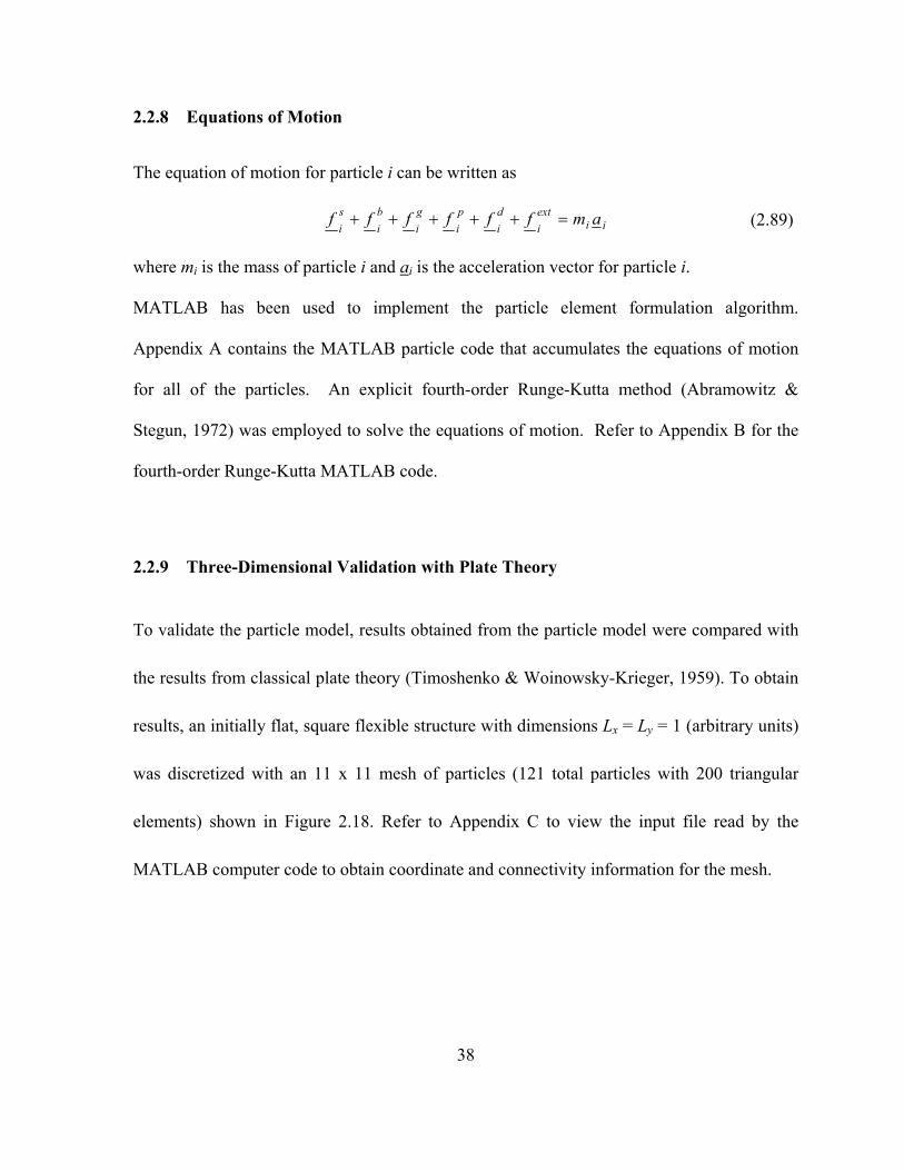
Figure 2.18. Flexible Structure: Triangular Mesh

The flexible structure was simply supported on all four edges. A point load P was applied at

the center, shown in Figure 2.19.

40

Figure 2.19. Simply Supported on all Four Sides, Center Point Load

The formula for the deflection of such a square plate from the classical theory is

terms

1m

terms

1n y

y

x2

2y

2

2x

2

yx

yx4z L

yLn

L

xm

L

n

L

m

L

n

L

m

DLL

P4 # # )(sinsin

sinsin

(2.90)

where D is the bending/flexural rigidity of the plate, ζ is the x-location of the load point, η is

the y-location of the load point, while x and y are the coordinates of the point in question. For

the maximum deflection at the center, equation 2.90 reduces to

terms

1m

terms

1n2224

2x

znm

1

D

PL4 # #

(2.91)

The data used for the particle model was: P = 1, m =1, c = 0.5, Lx = Ly = 1, k0 = 1, kb = 0.0345

(arbitrary units). The value of k0 was chosen arbitrarily while the kb value was chosen to limit

41

the maximum particle model deflection to 0.1 ≤ 0.001 for the given applied load P. The

value of D was adjusted in computation of the theoretical deflection so that the center

deflection predicted by plate theory matched the particle model result (both giving δz =

0.1004). The required value for D was 0.11509.

Table 2.3 shows the results of the particle model deflection compared with the theoretical

results.

Table 2.3: Square Plate, Deflection Results, Comparing Particle Model with Plate Theory

Particle Model Plate Theory

x y δz δz % Error

0 0.5 0.0000 0.0000 0.0% 0.1 0.5 0.0232 0.0221 4.8% 0.2 0.5 0.0474 0.0540 12.2% 0.3 0.5 0.0704 0.0796 11.5% 0.4 0.5 0.0902 0.0952 5.3% 0.5 0.5 0.1004 0.1004 0.0% 0.6 0.5 0.0902 0.0952 5.3% 0.7 0.5 0.0704 0.0796 11.5% 0.8 0.5 0.0474 0.0540 12.2% 0.9 0.5 0.0232 0.0221 4.8% 1 0.5 0.0000 0.0000 0.0%

Table 2.3 shows the deflection values for the particles along the line y = 0.5. Since the

deflection at the center was forced to be equal for plate theory and the particle model, a 0.0 %

error is shown in Table 2.3 at the center of the plate. Also, since all four edges were simply

supported, the deflection of the two edge particles located along the line y = 0.5 was also

zero. The maximum error occurs at x = 0.2 and x = 0.8 with just over 12 % error. One major

42

assumption with plate theory is it is based solely on bending stiffness; membrane (stretching)

stiffness is neglected. When attempting to use the particle model with k0 = 0, the model did

not produce favorable results. Therefore, stretching stiffness was included in the model

which may provide an explanation for the discrepancies between plate theory and the particle

model. Figure 2.20 shows a graphical representation of the comparison of the deflection

curves shown in Table 2.3.

Figure 2.20. δz/Lx vs. x: Particle Model Compared with First 11 Terms of Plate Theory (for y = 0.5)

Figure 2.20 shows the particle model curve matches the plate theory curve between the edges

very closely. The points on the curves which do not match exactly are highlighted by the

percent error values reported in Table 2.3.

0

0.02

0.04

0.06

0.08

0.1

0.12

0 0.2 0.4 0.6 0.8 1 1.2

δz /Lx

x

δz /Lx vs. x

Plate Theory 11 Terms

Particle Model

43

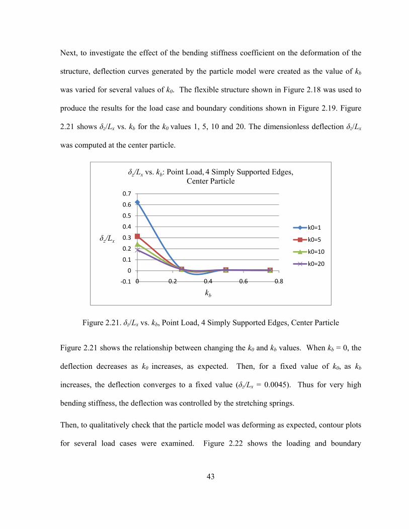
Next, to investigate the effect of the bending stiffness coefficient on the deformation of the

structure, deflection curves generated by the particle model were created as the value of kb

was varied for several values of k0. The flexible structure shown in Figure 2.18 was used to

produce the results for the load case and boundary conditions shown in Figure 2.19. Figure

2.21 shows δz/Lx vs. kb for the k0 values 1, 5, 10 and 20. The dimensionless deflection δz/Lx

was computed at the center particle.

Figure 2.21. δz/Lx vs. kb, Point Load, 4 Simply Supported Edges, Center Particle

Figure 2.21 shows the relationship between changing the k0 and kb values. When kb = 0, the

deflection decreases as k0 increases, as expected. Then, for a fixed value of k0, as kb

increases, the deflection converges to a fixed value (δz/Lx = 0.0045). Thus for very high

bending stiffness, the deflection was controlled by the stretching springs.

Then, to qualitatively check that the particle model was deforming as expected, contour plots

for several load cases were examined. Figure 2.22 shows the loading and boundary

‐0.1

0

0.1

0.2

0.3

0.4

0.5

0.6

0.7

0 0.2 0.4 0.6 0.8

δz/Lx

kb

δz/Lx vs. kb: Point Load, 4 Simply Supported Edges, Center Particle

k0=1

k0=5

k0=10

k0=20

44

conditions along with the contour plot of the final deformed mesh for the given load-case.

The parameters used were: P = 1, Lx = Ly = 1.

Figure 2.22. Simply Supported on Two Edges with a Center Point Load

Examining the final deformed shape of the particle mesh makes it easier to visualize how the

mesh deforms due to an applied point load. For a center point load applied in the positive z-

45

direction with two simply supported edges, Figure 2.22 shows the contour plot of the final

deformed shape of the mesh. The largest deflection (shown in red) occurred at the point of

the applied load, as expected. The deformation of the mesh was symmetric, with the smallest

deflection occurring at the two simply supported edges (shown in blue).

In the next case, the particle mesh was simply supported on two edges with a line load along

x = 0.5 in the positive z-direction. Figure 2.23 shows the loading and boundary conditions

along with the contour plot of the final deformed mesh for this case. The parameters used

were: P = 1, Lx = Ly = 1.

46

Figure 2.23. Simply Supported on Two Edges with a Line Load

Figure 2.23 shows the maximum deflection occurred along the line of applied load where the

deflection was also uniform as expected. Again, the minimum deflection occurs at the two

simply supported edges and the deformation of the mesh was symmetric.

47

Then, the next load-case was used to validate the particle model with plate theory. The mesh

was simply supported on all four edges with a center point load applied in the positive z-

direction. Figure 2.24 shows the loading and boundary conditions along with the final

contour plot of the deformed mesh for this case. The parameters used were: P = 1,

Lx = Ly = 1.

Figure 2.24. Simply Supported on all Four Edges with a Center Point Load

48

As expected, the largest deflection occurred at the point of the applied load and the

deformation of the mesh was symmetric. The smallest deflection occurred at all four simply

supported edges.

Finally, the last case was a mesh simply supported on all four edges with a line load applied

at x = 0.5 in the positive z-direction. Figure 2.25 shows the loading and boundary conditions

along with the contour plot of the final deformed mesh for this case. The parameters used

were: P = 1, Lx = Ly = 1.

49

Figure 2.25. Simply Supported on all Four Edges with a Line Load

Figure 2.25 shows the largest deflection occurred for three particles along the line of the

applied load but deflection was limited near the edges due to the simply supported condition.

The deflection differs in Figure 2.25 from that of Figure 2.24 because the load was

distributed along the line x = 0.5, rather than applying the full magnitude of the load at the

50

center particle. This qualitative analysis showed that for a set of load-cases, the particle

model deformed as expected.

51

3 Contact Formulation

One of the project goals was to account for the interaction between a rigid impactor, modeled

as a moving surface meshed with triangular elements, with a flexible structure, also modeled

with a triangular mesh of particles. The positions of the impactor vertices are tracked to

detect whether they have crossed any elements on the flexible structure. The flexible

structure was modeled with the particle method formulation discussed in the previous

chapter. The basic contact detection scheme must determine whether the impactor vertices

have pierced structural elements, and if so, appropriate action must be taken.

Contact is often times a very difficult, yet very important issue. When speaking of contact,

there are generally two steps to every contact algorithm, contact detection and contact

correction. The algorithm described in this chapter uses a point-to-plane contact detection

scheme with an update made to the velocity of the element vertices when contact has been

detected.

3.1 Contact Detection

The contact algorithm uses a point (impactor vertices)-to-plane (structural element) detection

scheme. In order to detect contact between the impactor vertices and the flexible structure

elements, it must first be determined which particle element, if any, an impactor vertex has

crossed. In terms of computer programming, the contact algorithm is computationally

demanding; requiring a loop over all possible flexible structure contact elements within a

loop over all impactor vertices. The nearest projection of an impactor vertex onto a structural

52

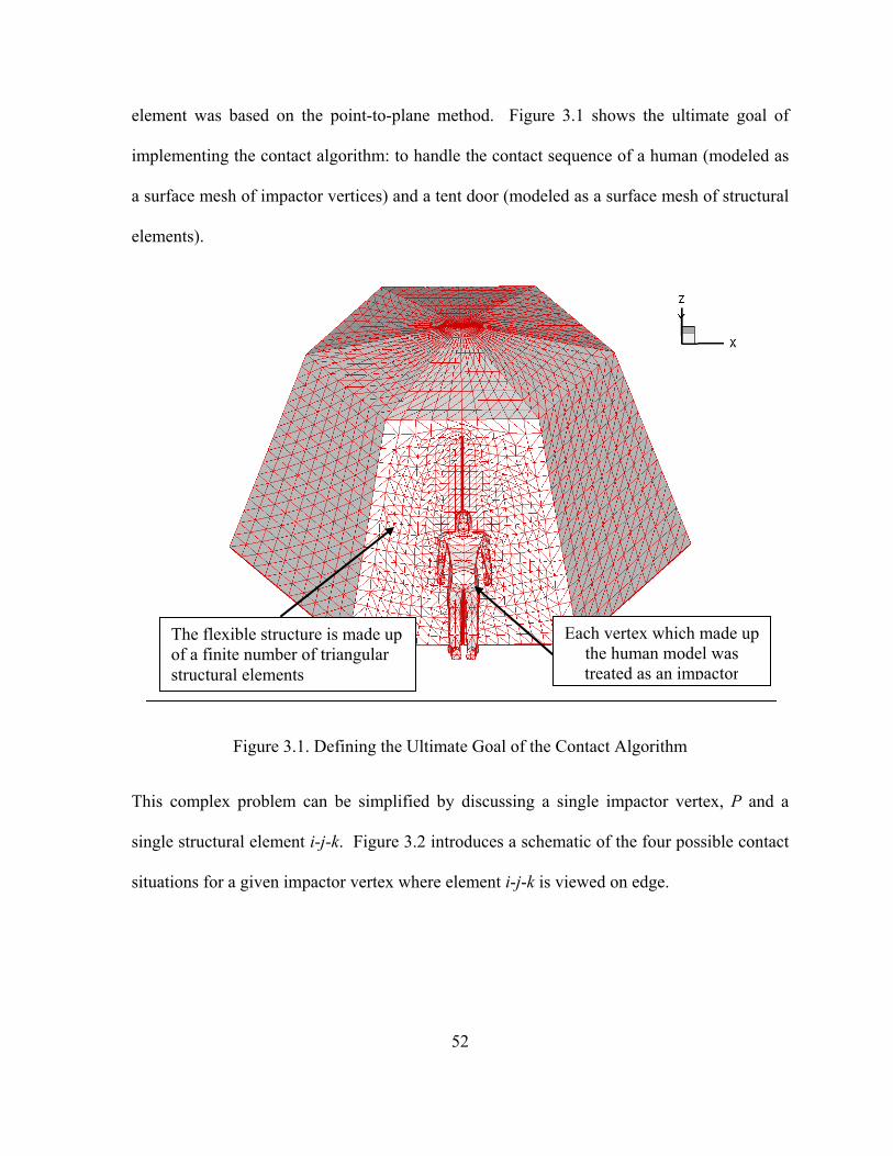
element was based on the point-to-plane method. Figure 3.1 shows the ultimate goal of

implementing the contact algorithm: to handle the contact sequence of a human (modeled as

a surface mesh of impactor vertices) and a tent door (modeled as a surface mesh of structural

elements).

Figure 3.1. Defining the Ultimate Goal of the Contact Algorithm

This complex problem can be simplified by discussing a single impactor vertex, P and a

single structural element i-j-k. Figure 3.2 introduces a schematic of the four possible contact

situations for a given impactor vertex where element i-j-k is viewed on edge.

Each vertex which made up the human model was treated as an impactor

The flexible structure is made up of a finite number of triangular structural elements

53

Figure 3.2. Possible Contact Situations

Figure 3.2.a. shows a typical impactor vertex approaching the structural element i-j-k. The

projection of this vertex would lie within a structural element on the flexible structure mesh.

At this point, since the impactor has not yet crossed the element, contact should not be

detected. At some later time, after having crossed the element this impactor vertex would be

at a position as in Figure 3.2.b. Again, the projection of this vertex would lie within a

structural element on the flexible structure mesh and contact should be detected.

Determining whether contact has occurred will be described in more detail in Section 3.2.

Then, at some time later than that of Figure 3.2.b. the impactor vertex would be at a position

as in Figure 3.2.c. At this time, the projection of the impactor vertex would not lie within a

structural element on the flexible structure mesh; contact should no longer be detected.

Finally, Figure 3.2.d. shows an impactor vertex whose projection does not lie within a

structural element on the flexible structure mesh and whose projection will never lie within a

structural element. As a result, contact should never be detected. Figure 3.2 illustrates the

54

possible contact situations which had to be accounted for when developing the contact

algorithm.

Figure 3.3 shows vertices i, j, and k of a typical structural element. By definition these three

vertices lie in a plane, shown in grey in the figure.

Figure 3.3. Plane ijk

Plane ijk is the plane defined by element i-j-k in the xyz-coordinate system. The position

vectors of points i, j, and k are xi, xj, and xk, respectively where

ziyixii ezeyexx (3.1)

zjyjxjj ezeyexx (3.2)

55

zkykxkk ezeyexx (3.3)

The position vector of impactor vertex P is P where

zzyyxx ePePePP (3.4)

Then, v1 is a vector which points from vertex i to j, v2 is a vector which points from vertex i

to k, and v3 is a vector which points from vertex j to k, i.e.

zijyijxijij1 ezzeyyexxxxv )()()( (3.5)

zikyikxikik2 ezzeyyexxxxv )()()( (3.6)

zjkyjkxjkjk3 ezzeyyexxxxv )()()( (3.7)

The unit normal to element i-j-k, pnorm, is found by taking the cross product of v1 and v2. Note

that the unit normal pnorm discussed here in the contact development chapter is equivalent to

n124 or n234 developed in the three-dimensional bend formulation (Section 2.2.2).

21

21znormzynormyxnormxnorm vv

vvepepepp

21

zx2y1y2x1yz2x1x2z1xy2z1z2y1

norm vv

evvvvevvvvevvvvp

)()()(

(3.8)

Figure 3.4 illustrates the closest projection of point P on the plane defined by element i-j-k.

This point on the plane is denoted Q.

56

Figure 3.4. Closest Projection of Point P onto the Plane

The vector viP which points from vertex i to point P is calculated according to

zizyiyxixiiP ezPeyPexPxPv )()()( (3.9)

Then, the vector which points from Q to P along the normal direction pnorm is

normiPnormzQPzyQPyxQPxQP pvpevevevv )( (3.10)

The position vector of point Q can be obtained from

QPvPQ (3.11)

The point Q does not necessarily lie within element i-j-k, only in the plane defined by

element i-j-k.

Before continuing with the development of the contact algorithm, it is useful to illustrate the

contact detection sequence. Figure 3.5 shows the before and after configurations of the

impactor vertex and the structural element during a typical contact detection sequence.

Providing a visual representation of the contact algorithm is helpful in improving the

understanding of the basic idea which defines contact.

57

Figure 3.5. Before and After Configurations used to Define Contact

Contact is defined when the relative orientation of the unit normal vector, pnorm and the

vector vQP changes. When this occurs, the impactor vertex is said to have “penetrated” the

structural element. Up until this point, it has not yet been defined in which structural element

58

contact occurs. It is necessary to determine which structural element, if any, contains the

projection Q of a given impactor vertex. Therefore, determining whether or not point Q lies

within element i-j-k is the next issue.

In order to do so, the distance from each vertex in element i-j-k to point Q is calculated.

zizyiyxixi ezQeyQexQxQiQ )()()( (3.12)

and

zjzyjyxjxj ezQeyQexQxQjQ )()()( (3.13)

and

zkzykyxkxk ezQeyQexQxQkQ )()()( (3.14)

Figure 3.6 shows the case when point Q is contained inside element i-j-k with vectors iQ, jQ,

and kQ defined along with the subdivided areas A1, A2, and A3.

Figure 3.6. Point Q Projected Inside Element i-j-k

The total area A for element i-j-k can be conveniently calculated with a cross product

59

zx2y1y2x1yz2x1x2z1xy2z1z2y121 evvvvevvvvevvvv

2

1vv

2

1A )()()( (3.15)

The three sub-areas defined by point Q and vertices i, j, k are

zxy1yx1yzx1xz1xyz1zy111 eiQviQveiQviQveiQviQv

2

1iQv

2

1A )()()( (3.16)

and

zx2yy2xyz2xx2zxy2zz2y22 eviQviQeviQviQeviQviQ2

1viQ

2

1A )()()( (3.17)

and

zxy3yx3yzx3xz3xyz3zy333 ejQvjQvejQvjQvejQvjQv2

1jQv

2

1A )()()( (3.18)

When point Q lies within element i-j-k, the total area A must be the same as the sum of the

sub-areas, i.e.

321 AAAA (3.19)

Figure 3.7 shows the case when point Q does not lie inside element i-j-k.

Figure 3.7. Point Q Lying Outside Triangle ijk

60

Now, area A1 is defined by triangle ijQ, A2 by triangle ikQ, and A3 by triangle jkQ. Then,

when point Q lies outside element i-j-k, the sum of the sub-areas is generally greater than A,

i.e.

AAAA 321 (3.20)

Before moving forward, it is necessary to determine which impactor vertices may be in

contact with which structural elements. In order to do so, the sub-areas defined by equations

3.16, 3.17, and 3.18 are compared with the total area given by equation 3.15. For a given

impactor vertex P, a search over the number of structural elements on the flexible structure

mesh is executed. The conditions which must be checked are:

1. If for impactor vertex P, A1+A2+A3 > A for all the structural elements, this impactor

vertex will not be in contact with any structural elements; the algorithm stops

checking the given impactor vertex for contact.

2. If for impactor vertex P, A1+A2+A3 > A, but all structural elements have not been

checked, the next structural element was checked.

3. If for impactor vertex P, A1+A2+A3 < A for a given structural element, then this

structural element was determined to be a potential contact element for the given

impactor vertex. If this was the case, the algorithm must continue checking for

contact.

Next, Table 3.1 describes several important variables used in the contact algorithm which

was coded using MATLAB. Provided are the variable name, the initial value, the index range

(for array variables), the possible range of values the variable can have, and a short

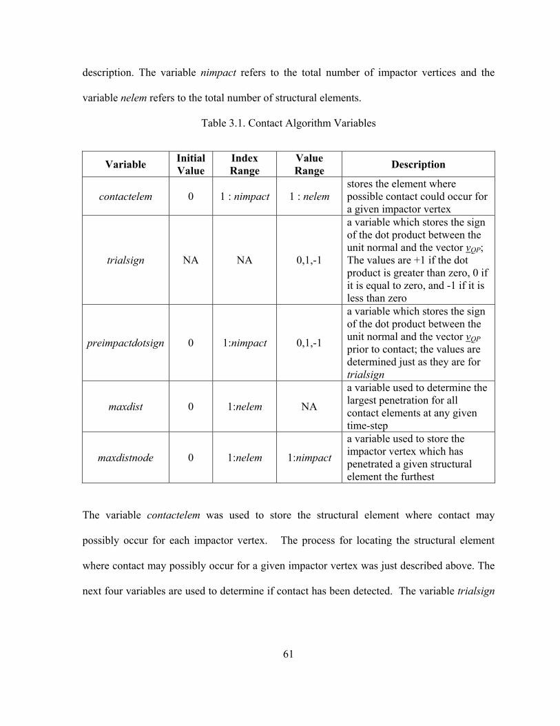
61

description. The variable nimpact refers to the total number of impactor vertices and the

variable nelem refers to the total number of structural elements.

Table 3.1. Contact Algorithm Variables

Variable Initial Value

Index Range

Value Range

Description

contactelem 0 1 : nimpact 1 : nelem stores the element where possible contact could occur for a given impactor vertex

trialsign NA NA 0,1,-1

a variable which stores the sign of the dot product between the unit normal and the vector vQP; The values are +1 if the dot product is greater than zero, 0 if it is equal to zero, and -1 if it is less than zero

preimpactdotsign 0 1:nimpact 0,1,-1

a variable which stores the sign of the dot product between the unit normal and the vector vQP prior to contact; the values are determined just as they are for trialsign

maxdist 0 1:nelem NA

a variable used to determine the largest penetration for all contact elements at any given time-step

maxdistnode 0 1:nelem 1:nimpact

a variable used to store the impactor vertex which has penetrated a given structural element the furthest

The variable contactelem was used to store the structural element where contact may

possibly occur for each impactor vertex. The process for locating the structural element

where contact may possibly occur for a given impactor vertex was just described above. The

next four variables are used to determine if contact has been detected. The variable trialsign

62

was assigned the value of the sign (+1, -1, 0) of the dot product between the unit normal

vector, pnorm and the vector vQP. Then, preimpactdotsign (stores the sign of the dot product

between the unit normal vector, pnorm and the vector vQP prior to contact; shown in the before

contact configuration of Figure 3.5) was compared to trialsign to determine whether an

impactor vertex has penetrated a structural element in any given time-step. If this was the

case, contact has been detected. Once contact had been detected, it was important to locate

the impactor vertex which had penetrated a given structural element the furthest. This was

done using the variable, maxdist, which was assigned the value of the distance from point Q

to point P, | vQP | for the impactor vertex which has penetrated the structural element the

furthest. The final variable, maxdistnode, was assigned the index value of the impactor

vertex which has penetrated the structural element the furthest. These variables are used to

determine which impactor vertices are in contact with which structural elements.

After determining the projection Q of impactor vertex P lies within element i-j-k, pnorm∏ vQP

was calculated and stored at each time-step.

)()()( QPznormzQPynormyQPxnormxQPnormvpvpvpvp (3.21)

The variable trialsign is simply the sign of the above dot product

QPnormvpsigntrialsign (3.22)

Then, the following conditions are checked to determine if contact has been detected:

Condition 1. If preimpactdotsign for impactor vertex P is equal to zero, the value of trialsign

is assigned to preimpactdotsign. There is no contact detected so the algorithm

continues checking the next impactor vertex.

63

Condition 2. If preimpactdotsign equals trialsign for impactor vertex P, there is no contact

detected so the algorithm continues checking the next impactor vertex.

Condition 3. If preimpactdotsign does not equal trialsign for impactor vertex P, contact has

been detected.

Note that multiple impactor vertices can make contact with a given element i-j-k. Figure 3.8

shows a schematic of this contact situation where element i-j-k is viewed on edge.

Figure 3.8. Multiple Contact Detections for Element i-j-k

As a result of the situation described by Figure 3.8, a sequence of checks was required to

determine which impactor vertex had penetrated element i-j-k the furthest. The checks

proceed in the following order,

a. If maxdistnode for element i-j-k is equal to zero (i.e. maxdistnode has not been

overwritten yet), maxdistnode for element i-j-k is set equal to impactor vertex

P and maxdist for element i-j-k is set equal to | vQP |. At this time, impactor

64

vertex P is the only impactor vertex to make contact with element i-j-k (since

maxdistnode was still equal to zero). The algorithm continues checking the

next impactor vertex, unless P is the final impactor vertex.

b. If | vQP | is less than maxdist for element i-j-k, another impactor vertex has

penetrated further than impactor vertex P. As a result, contact from impactor

vertex P will not be treated by the contact algorithm. The algorithm continues

checking the next impactor vertex, unless impactor vertex P is the final

impactor vertex.

c. If | vQP | is greater than maxdist for element i-j-k, maxdistnode for element

i-j-k is set equal to impactor vertex P and maxdist for element i-j-k is set equal

to | vQP |. At this time, impactor vertex P has penetrated element i-j-k the

furthest. The algorithm continues checking the next impactor vertex, unless

impactor vertex P is the final impactor vertex.

The algorithm described above identifies which impactor vertices are in contact with which

structural elements. Also, the impactor vertex which penetrates a given structural element

the furthest has been identified.

65

3.2 Contact Update

After determining which impactor vertices were in contact with which structural elements, it

was necessary to incorporate a contact update scheme. The correction scheme used by the

contact algorithm was one which updates the velocity components of the vertices i, j, k

depending on the impactor velocity. The basic idea of the contact update scheme used by the

contact algorithm was that collisions were inelastic and frictionless. As a result, only the

normal component of the impactor vertex velocity, termed vnorm, was used for updating

structural element velocities. Only structural elements which were found to have a

penetrating impactor vertex were updated. If a structural element had multiple penetrating

impactor vertices, only the impactor vertex which penetrated the structural element the

furthest was used to update velocities. The component of the impactor velocity vector along

the contacted element normal direction is

normnormimpactznormzynormyxnormxnorm ppvevevevv )( (3.23)

where vimpact is the velocity vector of the relevant impactor vertex.

The next step was to update the vertex velocities of contacted element i-j-k to account for the

interaction with the impactor vertex. Since the collisions were inelastic and frictionless,

contact with a structural element did not affect the motion of the impactor vertices. Also,

contact was only detected after an impactor vertex had penetrated a structural element, so the

position of the structural element would always lag behind that of the impactor vertex.

Therefore, an adjustable parameter b was used to enforce the compatibility of positions of the

impactor and structural element vertices at t = t + Δt. Figure 3.9 shows ttinx , , the predicted

66

position of the impactor vertex, ttsnx

, the predicted position of the structural element vertex,

tinx , the current position of the impactor vertex, t

snx , the current position of a structural

element vertex, and pnorm is the unit normal vector to structural element i-j-k. The time-step is

denoted Δt. A coordinate along the normal direction is denoted xn. The structural element

shown in Figure 3.9 is viewed on edge.

Figure 3.9. Current and Predicted Impactor and Structural Element Vertex Positions

The predicted positions of the impactor and structural element vertex are given by

67

tvxx normt

intt

in ,, (3.24)

and

tvbxx normt

sntt

sn ,, (3.25)

Since the impactor vertex moves at constant velocity its updated position can be predicted

exactly, while the calculation of the updated position of the structural vertex is influenced by

the mass and stiffness of surrounding elements and is hence only an approximation.

Equating the positions of the impactor vertex and the structural element vertex using

equations 3.24 and 3.25 gives

tvbxtvx normt

snnormt

in ,,

(3.26)

And it follows that

1bvtxx normt

snt

in ,, (3.27)

Finally

1

tv

xxb

norm

tsn

tin

,,

(3.28)

or,

1

tv

maxdistb

norm

(3.29)

Given the situation when there was almost solely sliding contact (i.e. the unit normal was

almost perpendicular to the impactor velocity); b can get very large and cause stability issues.

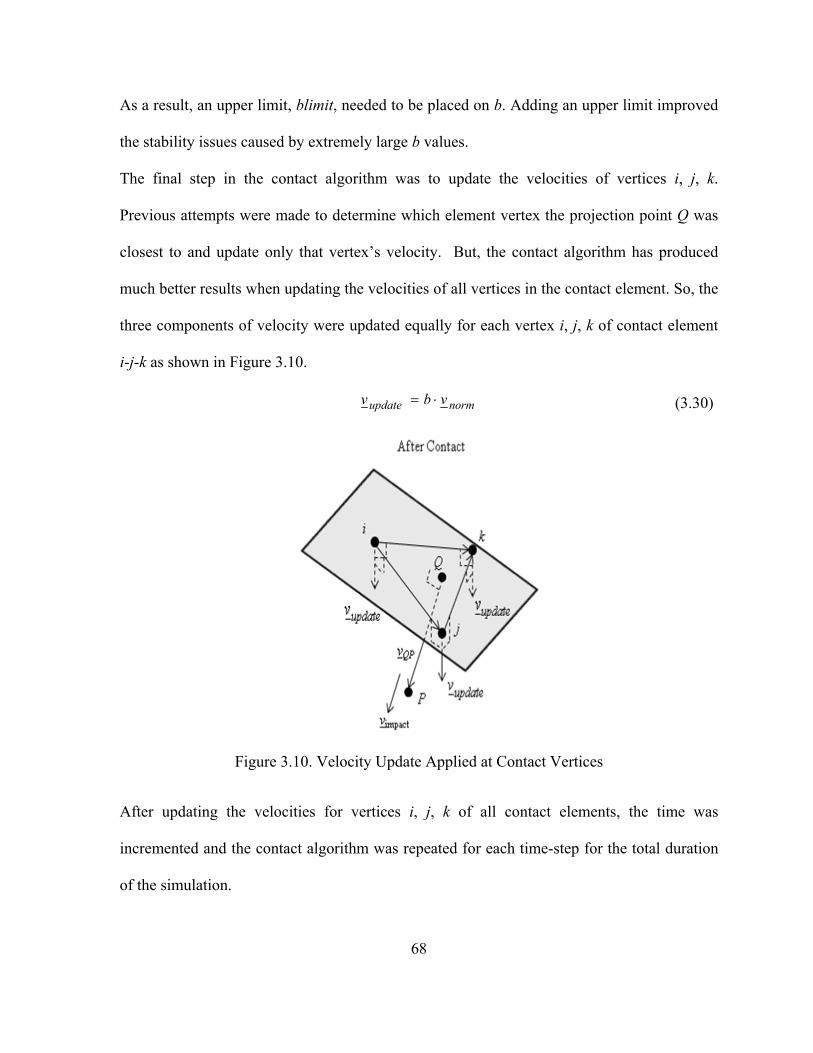
68

As a result, an upper limit, blimit, needed to be placed on b. Adding an upper limit improved

the stability issues caused by extremely large b values.

The final step in the contact algorithm was to update the velocities of vertices i, j, k.

Previous attempts were made to determine which element vertex the projection point Q was

closest to and update only that vertex’s velocity. But, the contact algorithm has produced

much better results when updating the velocities of all vertices in the contact element. So, the

three components of velocity were updated equally for each vertex i, j, k of contact element

i-j-k as shown in Figure 3.10.

normupdate vbv (3.30)

Figure 3.10. Velocity Update Applied at Contact Vertices

After updating the velocities for vertices i, j, k of all contact elements, the time was

incremented and the contact algorithm was repeated for each time-step for the total duration

of the simulation.

69

3.3 Contact Algorithm: Efficiency Improvement Methods

Computation times were greatly affected by the contact detection algorithm. The more

structural elements the algorithm had to check on a flexible structure, the more time it took to

complete. With that idea in mind, it is useful to refer back to Figure 3.1 which shows the

overall goal of the contact algorithm: to handle a contact sequence between a human and a

tent door. From Figure 3.1, as the human traverses the tent door, the impactor vertices will

not make contact with structural elements not located on the tent door. Although the contact

detection algorithm described above can handle checking all structural elements on the

flexible structure mesh, it is highly inefficient to do so. As a result, two methods are

described which limit the possible contact elements the contact algorithm must check. The

first method, referred to as “distance check method”, involves checking the distance from the

impactor vertex P to the centroid c of element i-j-k. The position vector c of the centroid of a

typical structural element i-j-k is

zzyyxx

kjiececec

3

xxxc

3

ezzzeyyyexxxc

zkjiykjixkji

(3.31)

Then, the distance Pcent from the impactor vertex P to c is

2zz2

yy2

xx cPcPcPPcent (3.32)

If this distance was greater than a specified distance referred to as distcheck, element i-j-k

was not a candidate for contact. To help simplify the explanation of this distance check

method, only the tent door from Figure 3.1 has been used to show the contact radius r (where

70

r = distcheck) in Figure 3.11. This method is not limited to the geometry shown in Figure

3.11 but this door is merely used to help clarify the method. Also, for simplification, a circle

rather than a sphere is used to describe the distance check method.

Figure 3.11. Front View of the Distance Check Method

If a structural element is not located within this circle, it is not a potential contact element.

Therefore, this method actually serves two purposes. It limits the number of potential contact

elements for a given impactor vertex while also forcing an impactor vertex to be located

within this radius before the algorithm begins to consider it for contact.

The second method, referred to as “the box method”, involves placing a three-dimensional

box around a contact location. If all three vertices i, j, k of element i-j-k were not located

71

within this box, element i-j-k was not considered as a potential contact element. If a set of

coordinate limits were not specified, it was assumed the box was infinite in that coordinate

direction. Figure 3.12 shows a front view used to describe the box method.

Figure 3.12. Front-View of the Box Method

Figure 3.12 shows how the box method limits possible contact elements by putting an upper

and lower limit on the three coordinate directions, x, y, and z.

Adding these two efficiency improvement methods to the contact algorithm has significantly

cut down on computation time while not compromising the simulation results.

72

4 Fabric Material Properties

This chapter outlines the procedure to convert experimentally determined fabric mechanical

properties to effective stiffness values useful to the particle model. It was desirable to model

actual fabric materials in the MATLAB computer code simulations. The benefits to doing so

were the units were no longer arbitrary and the simulations could model actual fabric

materials. The necessary properties which must be input to the MATLAB computer code are

the mass per unit area *, the mesh size dependent stretching stiffness coefficient k0, and the

bending stiffness coefficient kb. In order to measure the mechanical properties of the fabric,

a cantilever bending test was used. While it was possible to directly obtain * from the test,

the procedure to convert the mechanical property obtained from the cantilever bending test to

the useful k0 stiffness coefficient is described. Then, as an example, the procedure was

carried out for a military grade canvas material and the results are provided. It was not

possible to obtain the kb value directly from performing the cantilever bending test. As a

result, the procedure to set the value of the bending stiffness is also described.

4.1 Cantilever Bending Test

For the validation cases discussed in Chapter 2, arbitrary mass, stiffness, damping, and

external force values were used to validate the MATLAB computer code. In doing so, the

time, length, and force units were also arbitrary. Although a consistent set of units was

implied, it was desirable to incorporate the capability to model actual fabric materials with

actual values for mechanical properties. A sample of military grade canvas material was

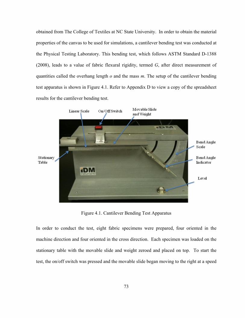
73

obtained from The College of Textiles at NC State University. In order to obtain the material

properties of the canvas to be used for simulations, a cantilever bending test was conducted at

the Physical Testing Laboratory. This bending test, which follows ASTM Standard D-1388

(2008), leads to a value of fabric flexural rigidity, termed G, after direct measurement of

quantities called the overhang length o and the mass m. The setup of the cantilever bending

test apparatus is shown in Figure 4.1. Refer to Appendix D to view a copy of the spreadsheet

results for the cantilever bending test.

Figure 4.1. Cantilever Bending Test Apparatus

In order to conduct the test, eight fabric specimens were prepared, four oriented in the

machine direction and four oriented in the cross direction. Each specimen was loaded on the

stationary table with the movable slide and weight zeroed and placed on top. To start the

test, the on/off switch was pressed and the movable slide began moving to the right at a speed

74

of 120 mm/min. The machine was stopped by pressing the on/off switch when the fabric

touched the bend angle indicator as shown in Figure 4.2.

Figure 4.2. Overhang Length of the Fabric

The value measured for each specimen was the overhang length, o (units millimeters). Four

overhang lengths were recorded for each specimen, specifically both ends, top, and bottom.

The overhang length was obtained by directly reading the value on the linear scale shown in

Figure 4.1 after the specimen first made contact with the bend angle indicator. Note that as

required by the ASTM standard, the bend angle indicator was set to an angle of 41.5°. These

four overhang lengths were averaged for each specimen to obtain the measured overhang

length.

After finding the overhang lengths, the eight specimens were placed on a scale and weighed

to the nearest thousandth of a gram. The total area of the specimens was 64 in2. In order to

calculate G, a mass per unit area value W was needed to be expressed in mg/cm2 units.

Therefore, the mass of the fabric divided by the area expressed in g/in2 was converted to

mg/cm2. The resulting value was W = 37.79 mg/cm2.

75

The bending length, c, is defined by

2

oc (4.1)

After obtaining the mass per unit area and the bending length, the flexural rigidity G was

computed according to the ASTM standard by means of

3cWG (4.2)

A flexural rigidity value was computed for each specimen in both fabric directions. These

four values were then averaged to yield a final flexural rigidity value of the fabric for each

machine direction.

After calculating the flexural rigidity, the interest was in converting to the more useful

parameter E, the elastic modulus (or Young’s modulus). Young’s modulus was used to tune

the stiffness values used in the MATLAB computer code.

Using the large deflection theory for a cantilever beam based on Rohde’s (1953) article, the

bend angle θ during the ASTM test corresponds to

L

L

x

ytan (4.3)

where yL and xL are the vertical and horizontal positions of the deflected beam, respectively.

Using the chart on page 338 of the Rohde paper, the ratio of yL/xL is equal to tan (41.5°) when

8

EI

wL 3

(4.4)

where w is the weight per unit length, L is the beam length, and EI is the bending stiffness.

For the cantilever bending test, L = o and o = 2c. Plugging 2c into equation 4.4 yields

76

1

EI

wc 3 (4.5)

where wc3 is the flexural rigidity, since w = W when the sample width is 1 inch. Therefore,

3wcEI (4.6)

where I is the moment of inertia of the test strips ( rectangular cross-section b × t). Therefore,

12

btI

3

(4.7)

where b is the specimen width and t is the thickness. Finally,

I

wcE

3 (4.8)

Thus, it is possible to convert from a measured flexural rigidity value G to Young’s modulus

E.

4.2 Obtaining the k0 Stiffness Coefficient

The particle stretch and bend stiffness coefficients, k0 and kb, cannot be obtained directly

from the test specimen or from the cantilever bending test. Instead, an indirect calculation

approach was employed.

After using the cantilever bending test to obtain Young’s modulus, the equation

AE

FL (4.9)

was used to determine the axial deflection of the test specimen. F is the applied axial load, L

is the length of the specimen, A is the cross sectional area, and E is Young’s modulus. After

77

determining the deflection for a given load, this same load and deflection were used to solve

for the stretching stiffness,

L

AEFk

(4.10)

The stretching stiffness coefficient used in the MATLAB computer code, k0 was calculated

according to

khk0 (4.11)

Thus a procedure has been developed to convert an experimentally measured mechanical

fabric property to the useful stretch stiffness coefficient used in the MATLAB computer

code.

4.3 Example: Canvas Tent Material

For the canvas material provided, the measured values obtained from the cantilever bending

test are shown in Table 4.1.

Table 4.1. Measured Properties

Property Value Force

(chosen arbitrarily) F = 1 lb

Length L = 8 in Width b = 1 in

Thickness t = 0.038 in Mass m = 15.6 g Area A = 0.038 in2

Mass per unit area * = 0.0024 slug/ft2 Flexural rigidity

(result of material test) G = wc3 = 0.002627 lb∏in

78

Then, the values calculated through the procedure described in Section 4.2 are provided in

Table 4.2.

Table 4.2. Calculated Properties

Property Equation Value Moment of Inertia (4.7) I = 4.57267E-6 in4

Young’s modulus (4.8) E = 574.5 lb/in2

Deflection (4.9) δ = 0.3665 in Stretch Coeff. (Actual) (4.10) k = 2.7285 lb/in Stretch Coeff. (Code) (4.12) k0 = 21.83 lb

The mass per unit area and the stretching stiffness coefficient are two of the properties

required to model fabric material using the particle method. These values were used in the

MATLAB computer code. The procedure to set the value of the bending stiffness, kb,

required to fully model the canvas material is outlined in Section 4.4.

4.4 Obtaining the Bending Stiffness Coefficient kb

After calculating k0 to be used in the MATLAB computer code, the final property needed to

model the canvas material is the bending stiffness, kb. In order to obtain this value, the

bending deflection was forced to match classical plate theory using a “tuning” approach. The

simply supported plate configuration used for the tuning approach is shown in Figure 4.3.

79

Figure 4.3. Simply Supported Rectangular Plate Used for the Tuning Approach

The deflection equation for plate theory (Timoshenko & Woinowsky-Krieger, 1959) is based

on rectangular plates. Figure 4.4 shows the particle mesh used to model a flat, flexible fabric

structure with dimensions Lx = 5.833 ft and Ly = 6.75 ft. The plate was discretized with a

23 x 23 mesh of particles, 529 total particles with 968 triangular elements.

80

Figure 4.4. Particle Mesh Used for Bending Stiffness Tuning

Plate theory provides an equation for transverse deflection of the plate.

terms

1m

terms

1n y

y

x2

2y

2

2x

2

yx

yx4z L

yLn

L

xm

L

n

L

m

L

n

L

m

DLL

P4 # # )(sinsin

sinsin

(4.12)

Using the first four terms of the series with the plate dimensions, equation 4.12 reduces to

81

D

P43360.max (4.13)

where P is the applied load and D is the bending/flexural rigidity of the plate defined as

)( 2

3

112

EtD

(4.14)

where E is Young’s modulus and t is the plate thickness, both obtained from the cantilever

bending test. Poisson’s ratio ν was assumed to be 0.3.

The only remaining unknown variable in equation 4.13 was the applied load P. For a number

of applied loads, the maximum deflection at the center of the mesh was calculated. A

convergence analysis was conducted to tune the kb value so the deflection of the MATLAB

computer code matched that of plate theory. Table 4.3 shows the data used to create Figure

4.5 which shows a plot of kb versus P for the six different cases.

Table 4.3. Data for kb vs. P

P (lb) kb (lb∏ft2) wcode (ft) wplate (ft)

0.00000075 0.0000046 0.001434 0.001352 0.0000005 0.000005 0.000897 0.000901 0.00000025 0.0000053 0.000447 0.00045 0.0000001 0.0000054 0.00018 0.00018

0.000000075 0.0000054 0.000135 0.000135 0.00000005 0.0000054 0.00009 0.00009

82

0.0000045

0.0000046

0.0000047

0.0000048

0.0000049

0.000005

0.0000051

0.0000052

0.0000053

0.0000054

0.0000055

0 0.0000002 0.0000004 0.0000006 0.0000008

k b(lb∏f

t2 )

P (lb)

kb vs. P

Convergence Analysis Kb value

Figure 4.5. kb vs. P

Figure 4.5 shows that as P decreases, the kb value approaches a constant value. From the

convergence study, kb = 0.0000054 lb∏ft2. One explanation for the very small applied loads

required to force the kb value to converge is the major assumption with plate theory which is

that it is based solely on bending stiffness; membrane (stretching) stiffness is neglected.

Therefore, in order to make the effect of the membrane stiffness negligible during a

simulation, a very small force must be applied. It is assumed then that the converged value is

the appropriate value to use in the particle model simulations to correctly model the bending

stiffness of the actual fabric material.

83

5 Results

This chapter presents the results obtained from seven simulations used to demonstrate the

utility of the MATLAB particle method code. Each of the seven cases was used to study a

different function of the code. A description of these seven cases follows:

Case 1: contact from a single impactor triangle with a hinged plate

Case 2: contact from multiple impactor triangles with a hinged plate

Case 3: a glancing blow contact event with a hinged plate

Case 4: contact of a sphere with a plate containing a slit

Case 5: a single soldier entering a full tent model without pressure

Case 6: a single soldier entering a full tent model with pressure

Case 7: three soldiers entering a full tent model without pressure

These cases range from the simplest contact event to a very complex contact interaction

including large structural deformations. All of the trial cases used the parameters reported in

Chapter 4 to model the actual canvas material. Since there are no clear cut forms of

validation, the results are presented qualitatively through snapshots of the animation

sequences and for the first and last cases, quantitatively as well in the form of plots and

figures.

84

5.1 Case 1: Single Impactor Triangle

The first case was the simplest case used to demonstrate the utility of the MATLAB

computer code. With the computer code having been configured to read and write STL files,

a triangle is the simplest possible impactor since STL files are presented in terms of triangles.

A single impactor triangle (dimensions lx = 0.3 ft, ly = 0.3 ft) made contact with a flexible

structure (Lx = 5.833 ft, Ly = 6.75 ft) discretized with a 23 x 23 mesh of particles, 529 total

particles with 968 triangular elements and hinged along the top edge. Refer to Appendix E

for the MATLAB code for this case. The x and y coordinates of the four corners of the

flexible structure and the vertices of the impactor triangle in the initial undeformed

configuration are shown in Figure 5.1. The initial configuration of the flexible structure was

located in the xy-plane. The impactor was moving in the negative z-direction with a constant

velocity vimpact.

85

Figure 5.1. Case 1 Initial Flexible Structure and Impactor Configuration

Figure 5.2 shows the input gravitational force (fgy), effective force due to pressure ( p

if ), and

velocity (vimpact) versus time for a given animation sequence. The gravitational force was

applied as a step function at time t = 0. The effective force due to pressure was applied as a

ramp function starting at time t = tp,start and ending at time t = tp,end, then held constant

thereafter. The impactor started to move stepwise at time t = tlag.

86

Figure 5.2. Forces and Velocity versus Time Plot

The numerical values of the parameters in the MATLAB particle code were: * = 0.0024

slug/ft2, k0 = 21.828 lb, kb = 0.0000054 lb∏ft2, c = 0.0005 lb∏s/ft, vimpact = -0.4 ft/s, gy =

-32.174 ft/s2. There was no effective force due to pressure applied for this simulation, p = 0

lb/ft2. The simulation had a total duration of 10 seconds with a time-step of Δt = 0.0004 s.

The time lag on the impactor was tlag = 0.1 s. STL files were output every 250 time-steps or

at a time interval of 0.1 s. Contact checking on the flexible mesh was only done in the range

-0.5 ft < y < 3 ft, for all x and z values (i.e. a horizontal strip). The distance check limit for

this simulation was distcheck = 1.5 ft. The final parameter was the limit on the adjustable

parameter, blimit = 40.

87

The simulation produced the time-lapse results shown in Figure 5.3. At t = 0 s, the initial

configuration of the impactor and flexible structure is shown. Gravity was activated during

the first time-step and the effects of this force are observed to damp to a steady-state value at

approximately t = 0.5 s. Then, at t = 1.2 s, the impactor first contacts the flexible structure.

In the images 3.6 s < t < 7.3 s contact is present. At some time after t = 7.3 s, contact is lost

and the impactor slides off the fabric. Finally, at t = 10 s the structure has returned to the

steady-state position under the influence of gravity only.

88

Figure 5.3. Single Impactor Triangle Animation Sequence

Then, Figure 5.4 shows the time-history plot for the x, y, z positions and velocities of the

mid-side of the bottom edge (vertex 276 with coordinates x = 2.9165, y = 0, z = 0). This

figure was included to provide a quantitative result for the animation sequence shown in

Figure 5.3. The results in Figure 5.4 coincide with Figure 5.3.

st 0 st 5.0

st 6.3st 2.1

st 10st 3.7

89

Figure 5.4. Time-History Plot for Structural Element Vertex 276

Also of interest was the maximum penetration value over the total duration of the simulation.

The results are shown in Figure 5.5.

90

Figure 5.5. Time-History Maximum Penetration

Note that the scale on the penetration axis is very small. Using as a characteristic length for a

triangular element, the max edge length, l = 0.4 ft. Figure 5.5 shows the maximum

penetration for the simulation was 4.38x10-4 ft. This value is 0.1% of the element size which

amounts to a very small penetration. The goal was to limit violations of the contact algorithm

and this case was able to achieve that goal. This case, involving a single impactor triangle

was used to initially demonstrate the utility of the MATLAB particle code. The results

provided valuable information about the code’s ability to handle a contact event.

91

5.2 Case 2: Multiple Impacts

Following a single impact event, this case looked at the ability of the MATLAB particle code

to handle multiple impacts from multiple impactors. This case used the same flexible

structure and material properties as Case 1. The use of impactor triangles was still present in

this case where five impactors moved with five different constant velocities in the negative z-

direction: vimpact1, vimpact2, vimpact3, vimpact4, and vimpact5. The x and y coordinates of the four

corners of the flexible structure and the vertices of the five impactor triangles in the initial

undeformed configuration are shown in Figure 5.6. Refer to Appendix F for the inputs to the

MATLAB computer code for this case and Appendix G for the impactor input file read by

the MATLAB computer code.

92


Referencing Figure 5.2 provides a better understanding of how the listed forces and velocities

were applied during the simulation.


slug/ft2, k0 = 21.828 lb, kb = 0.0000054 lb∏ft2, c = 0.0005 lb∏s/ft, vimpact1 = 0.55 ft/s, vimpact2 =

0.5 ft/s, vimpact3 = 0.4 ft/s, vimpact4 = 0.3 ft/s, vimpact5 = 0.1 ft/s, gy = -32.174 ft/s2. There was no

effective force due to pressure applied for this simulation, p = 0 lb/ft2. The simulation had a

total duration of 12 s with a time-step of Δt = 0.0004. The time lag on the impactors was tlag

93

= 0.1 s. STL files were output every 300 time-steps or at a time interval of 0.12 s. Contact

checking on the flexible mesh was only done in the range -0.5 ft < y < 1.8 ft, for all x and z

values (i.e. a horizontal strip). The distance check limit for this simulation was distcheck =

1.5 ft. The final parameter was the limit on the adjustable parameter, blimit = 40.


configuration of the impactors and flexible structure is shown. Gravity was activated during


approximately t = 0.5 s. At some time just prior to t = 1.32 s, impactors 1 and 2 make contact

with the flexible structure. Then, at t = 2.28 s, contact continues with all five impactors

making contact with the flexible structure. At approximately t = 4.56 s, impactor 1 slides off

the fabric but contact continues with the other four impactors. Then, at approximately t = 6.6

s, impactor 2 slides off the fabric and contact continues with the remaining three impactors.

Then, at some time before t = 7.08 s, the remaining impactors have slid off the fabric and

contact is lost. Finally, at t = 12 s the structure has returned to the steady-state position under

the influence of gravity only.

94

Figure 5.7. Multiple Impacts with Flexible Structure Animation Sequence

st 0 st 5.0

st 32.1 st 28.2

st 56.4 st 6.6

st 08.7 st 12

95

5.3 Case 3: Glancing Blow

After completing simulations involving single and multiple contacts, the next case looked at

a glancing blow provided by a single impactor triangle (same dimensions as Cases 1 and 2).

This case was important in determining whether the MATLAB particle code could handle

sliding contact. Again, this case used the same flexible structure and material properties as

Cases 1 and 2. The x and y coordinates of the four corners of the flexible structure and the

vertices of the impactor triangle in the initial undeformed configuration are shown in Figure

5.8. Refer to Appendix H for the inputs to the MATLAB computer code for this case.

96


The desired impact location for this case was 1 ft away from the initial impactor

configuration in the negative x-direction and 0.3 ft away in the negative z-direction. With the

respective distances to the impact location, the impactor was given constant velocities, vimpact1

in the negative x-direction and vimpact2 in the negative z-direction, forcing contact to occur at

this desired location to produce a glancing blow effect.


slug/ft2, k0 = 21.828 lb, kb = 0.0000054 lb∏ft2, c = 0.0005 lb∏s/ft, vimpact1 = 0.8 ft/s, vimpact2 =

97

0.24 ft/s, gy = -32.174 ft/s2. There is no effective for due to pressure applied for this

simulation, p = 0 lb/ft2. The simulation had a total duration of 8 s with a time-step of Δt =

0.0004. The time lag on the impactor was tlag = 0.1 s. STL files are output every 200 time-

steps or at a time interval of 0.08 s. Contact checking on the flexible mesh was only done in

the range -0.5 ft < y < 1.0 ft, for all x and z values (i.e. a horizontal strip). The distance check

limit for this simulation was distcheck = 1.2 ft. The final parameter was the limit on the

adjustable parameter, blimit = 75.


configuration of the impactor and flexible structure is shown. Gravity was activated during


approximately t = 0.5 s. Then, at t = 1.52 s, the impactor first contacts the flexible structure.

In the images 3.12 s < t < 4.8 s contact is present. At some time after t = 4.8 s contact is lost

and the impactor slides off the fabric. Finally, at t = 8 s, the structure has returned to the

steady-state position under the influence of gravity only.

98

Figure 5.9. Single Impactor Triangle, Glancing Blow Animation Sequence

This case was used to demonstrate the utility of the MATLAB particle code’s ability to

handle contact events involving sliding contact.

st 0 st 5.0

st 52.1 st 12.3

st 8.4 st 8

99

5.4 Case 4: Sphere Passing through a Plate with a Slit

For this case, a quadrilateral plate with a slit in the middle was created. The coordinates and

dimensions of the flexible structure in the initial undeformed configuration are shown in

Figure 5.10. The area and average element size of the quadrilateral plate were equivalent to

the flexible structure used in Cases 1 - 3. The plate was simply supported on all four edges,

allowing a sphere to pass through the slit. The importance of this simulation was it forced

the code to handle multiple impactors in the form of primitive shapes. Refer to Appendix I

for the inputs to the MATLAB computer code for this case.

100

Figure 5.10. Case 4 Initial Flexible Structure and Sphere Configuration

The quadrilateral plate tapers in width from the bottom edge to the top edge (dimensions Lxb

= 7 ft, Lxt= 4.66 ft, Lz = 6.75 ft). It is important to point out the orientation of the coordinate

system has changed for this case from that of Cases 1, 2, and 3. In this case, the plate was

slanted and was therefore located in all three planes, with the z-axis being the vertical axis.

The slit was centered along the line, x = 0, with a slit width, Lxs = 0.05 ft and a slit height Lzs

= 6.23 ft.

101

Since the orientation of the coordinate system has changed, Figure 5.2 has been replaced with

Figure 5.11 to reflect this change. Figure 5.11 shows the gravitational force (fgz), effective

force due to pressure ( p

if ), and velocity (vimpact) versus time for a given animation sequence.

Figure 5.11. Forces and Velocity versus Time Plot

The sphere moved with a constant velocity vimpact in the positive y-direction. The values used

for the parameters in the MATLAB particle code were: * = 0.0024 slug/ft2, k0 = 21.828 lb,

kb = 0.0000054 lb∏ft2, c = 0.0005 lb∏s/ft, vimpact = 0.5 ft/s, gz = 0 ft/s2. There was no effective

for due to pressure applied for this simulation, p = 0 lb/ft2. The simulation had a total

duration of 10 s with a time-step of Δt = 0.0002. The time lag on the sphere was tlag = 0.1 s.

102

STL files were output every 500 time-steps or at a time interval of 0.1 s. Contact checking

on the flexible mesh was only done in the range -0.4 ft < x < 0.4 ft, for all y and z values (i.e.

a vertical strip matching the slope of the plate). The distance check limit for this simulation

was distcheck = 0.7 ft. The final parameter was the limit on the adjustable parameter, blimit =

75.


configuration of the sphere and flexible structure is shown. The gravitational force was not

activated in this simulation therefore, there was no time lag needed for the effects of the

gravity force to damp to a steady-state value. The sphere was only delayed until t = 0.1 s,

when it begins to move. At t = 1.8 s, the sphere first contacts the flexible structure. In the

images 2.6 s < t < 3.9 s contact is present. At some time after t = 3.9 s, contact is lost and the

sphere passes through the slit. The image t = 4.2 s, shows the flexible structure returning to

its initial configuration. Finally, at t = 8 s, the structure has returned to its initial

configuration.

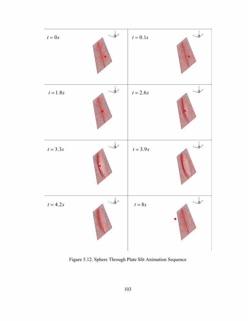
103

Figure 5.12. Sphere Through Plate Slit Animation Sequence

st 0

st 6.2

st 8

st 1.0

st 3.3 st 9.3

st 2.4

st 8.1

104

5.5 Case 5: Soldier Moving into Full Tent, No Pressure

The previous cases were used to demonstrate the utility of the contact algorithm, with the

goal to ultimately produce the results presented here in Case 5. This case presents a single

soldier impactor (referred to simply as “the soldier”) moving into the flexible fabric

hexagonal tent-like structure. The soldier model was represented as an STL surface mesh.

In the subsequent simulations, the soldier model was non-articulating, rather, all vertices on

the surface mesh moved with a constant velocity vimpact in the positive y-direction. The

overall soldier and tent dimensions are shown in Figure 5.13. These dimensions are merely

representative – they do not represent any particular human or conceived tent design. They

were chosen for illustrative purposes only. The coordinates of the corner base nodes, the

corner nodes at the top of the side panels, and at the peak of the tent are shown in Figure

5.14. In order to allow entry into the tent, one of the side panels was the slit quadrilateral

plate described in Case 4 (Figure 5.10). Refer to Appendix J for the inputs to the MATLAB

computer code for this case.

105

Figure 5.13. Initial Configuration of Soldier and Full Hexagonal-shaped Tent

7 ft

106

Figure 5.14. Pan View of Initial Soldier and Tent Configuration

Referring to Figure 5.11 provides a better understanding of when the given forces and

velocities were applied with respect to time.

The numerical values for the parameters used in the MATLAB particle code were: r* =

0.0024 slug/ft2, k0 = 21.828 lb, kb = 0.0000054 lb∏ft2, c = 0.0005 lb∏s/ft, vimpact = 0.8 ft/s, gz =

-32.174 ft/s2. There was no effective force due to pressure applied for this simulation, p = 0

lb/ft2. The simulation had a total duration of 10 s with a time-step of Δt = 0.0002. The time

107

lag on the soldier was tlag = 2.6 s. STL files were output every 500 time-steps or at a time

interval of 0.1 s. Contact checking on the flexible mesh was only done in the range -0.96 ft <

x < 1.02 ft, for all y and z values (i.e. a vertical strip matching the slope of the door). The

distance check limit for this simulation was distcheck = 0.7 ft. The final parameter was the

limit on the adjustable parameter, blimit = 75.


configuration of the soldier and the tent is shown. Gravity was activated during the first time-

step and the effects of this force are observed to damp to a steady-state value at

approximately t = 2.6 s, when the soldier begins moving toward the tent. Contact is first

made between the soldier and the tent at t = 5.3 s. In the images 5.8 s < t < 6.8 s contact is

present. At approximately t = 7 s, contact is lost and the soldier has completely traversed the

door and is inside the tent. Then, the image t = 7.4 s shows the door returning to its initial

position. Finally, at t = 10 s, the tent has returned to the steady-state position under the

influence of gravity only.

The animation sequence provided in Figure 5.15 qualitatively shows the MATLAB particle

code produced very realistic deformations during the contact sequence. Since the tent was

not pre-tensed, a sagging effect was created when gravity was activated. Note the sharp

indentations at the mid-sides of the tent’s straight edges reflect the effects of gravity on the

structural elements surrounding a simply supported edge vertex. Modeling the tent this way

was chosen to provide some rigidity to the tent frame. The frame rigidity can be changed by

varying the number of edge vertices which are simply supported.

108

Figure 5.15. Single Soldier Entering Full Hexagonal-Shaped Tent Animation Sequence

st 0 st 6.2

st 3.5 st 8.5

st 8.6 st 7

st 4.7 st 10

109

5.5.1 Comparing Particle Model Results with LS-DYNA

After completing Case 5, it was desirable to compare the results obtained from the particle

model with results obtained from the finite-element program, LS-DYNA. In order to do so,

the same soldier and flexible structure geometry shown in Figures 5.13 and 5.14 were used.

Since LS-DYNA reads and writes STL files, it was possible to directly import the soldier and

flexible structure STL files into the program. Then, the necessary fabric properties used in

Case 5 were directly input into LS-DYNA. The numerical values for the parameters used in

LS-DYNA were: mass density ρ = 0.757 slug/ft3, E = 82,728 lb/ft2, t = 0.00317 ft. The time

sequence for applying the gravity load and the human model motion were the same as Case

5. One property which was not directly analogous was the damping coefficient c. The global

damping coefficient value input in LS-DYNA was c = 0.9. LS-DYNA was executed in

explicit mode, whereby the time-step was controlled automatically. Figure 5.16 shows the

location of vertex 1872.

110

Figure 5.16. Location of Vertex 1872

Figure 5.17 provides a comparison of the position and velocity of vertex 1872 using a

position and velocity versus time plot from the MATLAB code (top) above the y-position

(middle) and y-velocity (bottom) versus time plots from LS-DYNA. For the MATLAB plot,

it was only the y-position (red solid line) and the y-velocity (red dotted line) which was

compared to the two LS-DYNA plots of the y-position and y-velocity. In Figure 5.17, the

general overall shape of the y-position and y-velocity curves were very similar. The LS-

DYNA curves were not as smooth as the particle model curves due to the difference in

111

damping coefficients. The peak of the curves and the steady-state positions were also very

similar.

Figure 5.17. Particle Model Comparison with LS-DYNA Vertex 1872

112

Figure 5.18. Comparison Between Particle Model and LS-DYNA Animation Sequence

113

st 0

st 6.2

st 3.5

st 8.5

st 0

st 6.2

st 3.5

st 8.5

114

st 8.6

st 7

st 10

st 4.7

st 8.6

st 7

st 10

st 4.7

115

The animation sequence shown in Figure 5.18 shows snapshots of the particle model

simulation (left) next to the LS-DYNA simulation (right). It is important to mention that

although these simulations used the same soldier and tent geometry and material properties,

there were some differences. First, the inability to match the damping coefficients caused

some differences during the animation sequence. Also, the flexible structure was not

constrained exactly the same in LS-DYNA as it was using the MATLAB computer code. In

LS-DYNA, the mid-sides of the bottom section of the tent were not constrained. This

eliminates what appears to be a sharp indentation in the mid-sides of the particle model

simulation. Also, at t = 7 s and t = 7.4 s, the soldier in the LS-DYNA simulation has

traversed the door earlier than in the particle model simulation. As a result, the deformation

of the flexible structure using the particle model does not appear exactly the same as the LS-

DYNA sequence. It is not exactly known why the models differ, but it may be that the LS-

DYNA model was not constrained as much as the particle model, which makes it less stiff or

it may be that LS-DYNA uses shell elements rather than the spring-mass system used by the

particle model. However, the importance of this comparison was to show that the simulation

using the MATLAB computer code produced very similar results to the LS-DYNA

simulation.

116

5.6 Case 6: Soldier Moving into Full Tent, with Pressure

Case 6 uses the same soldier and flexible structure geometry and parameters as Case 5, but

the results are presented with the addition of pressure. Referring to Figure 5.13 and Figure

5.14 provides the tent and soldier coordinates and dimensions. Applying pressure was an

important feature that the MATLAB particle code had to contain. As a result, this simulation

applied pressure while still handling a contact event. Referring to Figure 5.11 helps clarify

when the given forces and velocities were applied with respect to time. Refer to Appendix K

for the inputs to the MATLAB particle code for this case.

The numerical values for parameters used in the MATLAB particle code were: r* = 0.0024

slug/ft2, k0 = 21.828 lb, kb = 0.0000054 lb∏ft2, c = 0.0005 lb∏s/ft, vimpact = 0.8 ft/s, gz = -32.174

ft/s2. There was an effective force due to pressure applied for this simulation, p = 0.15 lb/ft2,

tp,start = 2.6 s and tp,end = 4.6 s. The simulation had a total duration of 12 s with a time-step of

Δt = 0.00015. The time lag on the soldier was tlag = 4.6 s. STL files were output every 800

time-steps or at a time interval of 0.12 s. Contact checking on the flexible mesh was only

done in the range -0.96 ft < x < 1.02 ft, for all y and z values (i.e. a vertical strip matching the

slope of the door). The distance check limit for this simulation was distcheck = 0.7 ft. The

limit on the adjustable parameter was, blimit = 75. An additional parameter was added for

this case, fixstretch = 0.75 ft. This parameter adjusted the tent peak vertex and the first ring of

vertices around the peak the value of fixstretch. This was done in the first time-step to pre-

tension the tent with the goal of limiting the stretch caused by the effective force due to

pressure.

117


configuration of the soldier and the tent is shown. Gravity was activated during the first time-

step and the effects of this force are observed to damp to a steady-state value at

approximately t = 2.6 s, when the pressure force is first applied. The pressure force reaches

its maximum value at t = 4.6 s, when the soldier begins moving toward the tent. Contact is

first made between the soldier and the tent at t = 5.2 s. In the images 7.1 s < t < 8.3 s contact

is present. At some point after t = 8.3 s, contact is lost and the soldier has completely

traversed the door and is inside the tent. The image at t = 8.8 s shows the door returning to its

position prior to contact. Finally, at t = 12 s, the tent is shown in the steady-state position

under the influence of gravity and pressure only.

In the image t = 12 s, the bottom of the tent door is shown folded over. It is desirable to

understand what is causing this result, but to this point, this cause has not been identified.

Also, with simulations involving pressure, the MATLAB particle code has an inability to

handle large pressure values. The deformation of the tent was very large even when very

small pressure values were applied. Not many simulations were conducted involving

pressure. As a result, additional simulations and analysis of how pressure is applied in the

contact algorithm would be necessary to fully understand the effective force due to pressure.

118

Figure 5.19. Single Soldier Entering Full Tent with Pressure Animation Sequence

st 0 st 6.2

st 6.4 st 2.5

st 1.7 st 3.8

st 8.8 st 12

119

5.7 Case 7: Soldier on a Gurney

The final case was the most complex contact interaction simulated by the MATLAB particle

model. The particle model had to handle large structural deformations. This case modeled

two soldiers carrying an injured soldier on a gurney; one soldier was placed at the head and

feet, respectively, of another soldier who was positioned face-up as if lying on a gurney.

Although the gurney was not modeled, this geometry replicates an entry event where two

soldiers would enter a tent carrying a third soldier on a gurney. The tent geometry and

properties used in this case were exactly the same as those used in Case 5 (Refer to Figures

5.13 and 5.14). The soldiers moved with a constant velocity vimpact in the positive y-direction.

The difference between this case and Case 5 was the use of three soldier impactors in this

case as opposed to one soldier in Case 5. Refer to Appendix L for the inputs to the MATLAB

computer code for this case.

Referring to Figure 5.11 provides a better understanding of when the given forces and

velocities were applied with respect to time.

The numerical values for parameters used in the MATLAB particle code were: r* = 0.0024

slug/ft2, k0 = 21.828 lb, kb = 0.0000054 lb∏ft2, c = 0.0005 lb∏s/ft, vimpact = 0.8 ft/s, gz = -32.174

ft/s2. There was no effective force due to pressure applied for this simulation, p = 0 lb/ft2.

The simulation had a total duration of 16 s with a time-step of Δt = 0.000125. The time lag

on the soldiers was tlag = 2.0 s. STL files were output every 1280 time-steps or at a time

interval of 0.16 s. Contact checking on the flexible mesh was only done in the range -0.96 ft

< x < 1.02 ft, for all y and z values (i.e. a vertical strip matching the slope of the door). The

120

distance check limit for this simulation was distcheck = 0.7 ft. The final parameter was the

limit on the adjustable parameter, blimit = 75.


configuration of the soldiers and the tent is shown. Gravity was activated during the first

time-step and the effects of this force are observed to damp to a steady-state value at

approximately t = 2.0 s, when the soldiers begin moving toward the tent. Contact is made

between the first soldier and the tent at t = 4.5 s. Contact continues with the first soldier until

some time after t = 6.25 s when the first soldier has completely traversed the door and is

inside the tent. As this occurs, contact is made between the second soldier, lying on his back,

and the tent. In the images 7.2 s < t < 8.8 s contact continues until some time after t = 8.8 s,

when contact with the second soldier is lost and this soldier has completely traversed the

door and is inside the tent as well. At some time after contact is lost with the second soldier,

contact is made between the third soldier and the tent. Contact continues with the third

soldier shown in the image at t = 12.8 s. At some time after t = 12.8 s, contact is lost and the

third and final soldier has completely traversed the door and is inside the tent. Finally, at t =

16 s, the tent is shown in the steady-state position under the influence of gravity only.

Qualitatively, Figure 5.20 shows the MATLAB particle code produces very realistic

deformations for the given entry event. For this event, the particle code handles a very

complex contact interaction between the tent and three soldiers which produces large

structural deformations.

121

Figure 5.20. Soldier on Gurney Entering Full Tent Animation Sequence

st 0 st 0.2

st 5.4 st 25.6

st 2.7 st 8.8

st 8.12 st 16

122

To quantitatively view the results, Figure 5.21 shows the time-history results for a mid-side

vertex located along the slit in the door (vertex 1872 with coordinates x = -0.025, y = -4.92,

z = 3.8).

Figure 5.21. Time-History Plot for Structural Element Vertex 1872

Figure 5.21 coincides with the results described in Figure 5.20. The maximum penetration

value over the total duration of the simulation is shown in Figure 5.22.

123

Figure 5.22. Time-History Plot of the Maximum Penetration

Figure 5.22 shows a long span of time when the penetration values were very small (i.e.

violations of the contact algorithm were minor). But, it is noted that the spike shown in

Figure 5.22 corresponds to a penetration value slightly larger than the element size. With the

contact algorithm used, penetration was the definition of contact. The goal was to limit this

penetration although violations do occur. This penetration value should not diminish the rest

of the result which produced very small contact violations.

124

6 Conclusions and Recommendations

6.1 Conclusions

A MATLAB computer code that implemented the particle-based formulation capable

of handling stretching and bending stiffness, external forces, and contact was created

and thoroughly tested. The computer code was validated where possible using

classical beam and plate theories.

A frictionless, inelastic collision/contact formulation was devised and implemented in

the MATLAB computer code. The contact algorithm has been tested on a wide range

of events simulating impact between rigid impactors and flexible structures and

appears to work dependably.

The computer code has been used to provide simulated ingress/egress events into a

tent-like structure.

The experimental procedure to measure actual fabric mechanical properties has been

documented.

The procedure to convert experimentally determined fabric mechanical properties to

effective stiffness values useful for the particle code simulations has been

documented.

The MATLAB code reads and writes STL files making it compatible with an

immersed boundary computational fluid dynamic code that can treat fluid-structure

interactions.

125

The results have been compared to simulations using the finite-element program, LS-

DYNA.

6.2 Recommendations for Future Research

Opportunities exist for making the code more efficient in order to seek reduced

computation time.

The stretching stiffness coefficient was successfully made independent of mesh size.

It would be very useful to determine a way to do the same with the bending stiffness

coefficient so it is not mesh-size dependent. This would eliminate the need for the

tuning approach.

It would be very interesting to take the output produced from the MATLAB computer

code and use it as input to the CFD code to obtain one-way coupled results. This was

the initial plan for this research and although the capability has now been developed,

this has not yet been completed.

Additional testing using different tent geometries, different fabric materials, and

different soldier configurations could be very valuable to the understanding of the

structural response over a range of parameters.

It is recommended that further comparisons between the particle model and LS-

DYNA be explored.

126

REFERENCES

Abramowitz, M., & Stegun, I. A. (Eds.). (1972). Handbook of Mathematical Functions with Formulas, Graphs, and Mathematical Tables. 55 , Applied Mathematics Series, 896. U.S. Department of Commerce: National Bureau of Standards. Baraff, D., & Witkin, A. (1998). Large Steps in Cloth Simulation. Computer Graphics Proceedings (SIGGRAPH 98), (pp. 43-54). Orlando. Baraff, D., Witkin, A., & Kass, M. (2003). Untangling Cloth. Annual Conference Proceedings (ACM SIGGRAPH 2003), (pp. 862-870). Bigliani, R., & Eischen, J. W. (2000). Collision Detection in Cloth Modeling. In D. H. House, & D. E. Breen, Cloth Modeling and Animation (pp. 197-217). Natick, Massachusetts: A K Peters. Breen, D. E., House, D. H., & Wozny, M. J. (1994). Predicting the Drape of Woven Cloth Using Interacting Particles. Computer Graphics Proceedings (SIGGRAPH '94) , 365-372. Choi, K.-J., & Ko, H.-S. (2002). Stable but Responsive Cloth. Computer Graphics Proceedings (SIGGRAPH), (pp. 604-611). (2006). Contact-Impact Algorithm. In LS-DYNA Theory Manual (pp. 26.1-26.46). Livermore, California: Livermore Software Technology Corporation. Eischen, J. W., Deng, S., & Clapp, T. G. (1996). Finite-Element Modeling and Control of Flexible Fabric Parts. Computer Graphics in Textiles and Apparel (IEEE Computer Graphics and Applications) , 71-80. Fontana, M., Rizzi, C., & Cugini, U. (2004). Physics-Based Modeling and Simulation of Functional cloth for Virtual Prototyping Applications. ACM Symposium on Solid Modeling and Applications (pp. 267-272). The Eurographics Association. Gere, J. M., & Timoshenko, S. P. (1997). Mechanics of Materials. Boston: PWS Publishing Co. Gu, X., Gortler, S. J., & Hoppe, H. (2002). Geometry Images. ACM Transactions on Graphics 2002, (pp. 355-361). Huh, S., Metaxas, D. N., & Badler, N. I. (2001). Collision Resolutioins in Cloth Simulation. IEEE Computer Animation Conference 2001.

127

O'Brien, J. F., Hodgins, J. K., & Zordan, V. B. (1997). Combining Active and Passive Simulations for Secondary Motion. Visual Proceedings (SIGGRAPH '97) (pp. 1-2). Los Angeles: ACM. Rohde, F. (1953). Large Deflections of a Cantilever Beam with Uniformly Distributed Load. Quart. Appl. Math. 11 , 337-338. (2008). Standard Test Method for Stiffness of Fabrics. D-1388. In ASTM International. West Conshohocken, PA: ASTM. Sul, I. H., & Kang, T. J. (2004). Improvement of Drape Simulation Speed using Constrained Fabric Collision. International Journal of Clothing Science and Technology , 43-50. Terzopoulos, D., & Fleischer, K. (1988). Modeling Inelastic Deformation: Viscoelasticity, Plasticity, Fracture. Computer Graphics (SIGGRAPH '88) vol. 22(4) (pp. 269-278). Atlanta: ACM. Terzopoulos, D., Platt, J. B., & Fleischer, K. (1987). Elastically Deformable Models. Computer Graphics (SIGGRAPH '87) vol. 21(4) (pp. 205-214). Anaheim: ACM. Timoshenko, S., & Woinowsky-Krieger, S. (1959). Simply Supported Rectangular Plates. In Theory of Plates and Shells (pp. 111-112). New York: McGraw-Hill. Volino, P., & Magnenat Thalmann, N. (2000). Implementing Fast Cloth Simulation with Collision Response. Proceedings of the Conference on Computer Graphics International (CGI-00), (pp. 257-268). Volino, P., & Magnenat-Thalmann, N. (1994). Efficient Self-Collision Detection on Smoothly Discretised Surface Animation Using Geometrical Shape Regularity. Computer Graphics Forum (Eurographics '94) (pp. 155-166). Blackwell Publishers. Zhang, D., & Yuen, M. M. (2000). Collision Detection for Clothed Human Animation. Proceedings of the 8th Pacific Graphics Conference on Computer Graphics and Application (PACIFIC GRAPHICS-00), (pp. 328-337). Zink, N., & Hardy, A. (2007). Cloth Simulation and Collision Detection using Geometry Images. Proceedings of the 5th International Conference on Computer Graphics, Virtual Reality, Visualisation and Interaction in Africa (SIGGRAPH 2007) (pp. 187-195). Grahamstown: ACM.

128

APPENDIX

129

A Equations of Motion Matlab Function Code

%Declaring variables used in both functions as global global d0 nnodes m c k0 kb fxext fyext fzext fixed coords NNM bend nconnect kap0 nelem vertex pmax tpstart tpend gx gy gz a dvdt=[]; %This must be uncommented for simulations involving pressure %for loop over the number of elements to get areas and normals used for %pressure loading % for ii=1:nelem % Ax=v(6*vertex(ii,1)-5); % Ay=v(6*vertex(ii,1)-3); % Az=v(6*vertex(ii,1)-1); % % Bx=v(6*vertex(ii,2)-5); % By=v(6*vertex(ii,2)-3); % Bz=v(6*vertex(ii,2)-1); % % Cx=v(6*vertex(ii,3)-5); % Cy=v(6*vertex(ii,3)-3); % Cz=v(6*vertex(ii,3)-1); % % v1=sqrt((Bx-Ax)^2+(By-Ay)^2+(Bz-Az)^2); % v1x=(Bx-Ax); % v1y=(By-Ay); % v1z=(Bz-Az); % % v2=sqrt((Cx-Ax)^2+(Cy-Ay)^2+(Cz-Az)^2); % v2x=(Cx-Ax); % v2y=(Cy-Ay); % v2z=(Cz-Az); % % pnorm(ii)=sqrt((v1y*v2z-v1z*v2y)^2+(v1z*v2x-v1x*v2z)^2+(v1x*v2y-

v1y*v2x)^2); % pnormx(ii)=(v1y*v2z-v1z*v2y)/pnorm(ii); % pnormy(ii)=(v1z*v2x-v1x*v2z)/pnorm(ii); % pnormz(ii)=(v1x*v2y-v1y*v2x)/pnorm(ii); % % elemarea(ii)=1/2*pnorm(ii); % end %Create a set of for loops to solve equations of motion for a number of desired particles %%%%%%%%%%%%%%%%%%%%%%%%%%%%%%%%%%%%%%%%%%%%%%%%% %Calculating the forces contributed due to stretching for ii=1:nnodes

130

ax=0; ay=0; az=0; if fixed(ii)==1 axx(ii) = 0; ayy(ii) = 0; azz(ii) = 0; continue end for jj=3:NNM(ii,2)+2 d0=sqrt((coords(NNM(ii,jj),1)-coords(NNM(ii,1),1))^2 +

(coords(NNM(ii,jj),2)-coords(NNM(ii,1),2))^2 + (coords(NNM(ii,jj),3)-coords(NNM(ii,1),3))^2);

d=sqrt((v(6*NNM(ii,jj)-5)-v(6*NNM(ii,1)-5))^2 + (v(6*NNM(ii,jj)-3)-v(6*NNM(ii,1)-3))^2 + (v(6*NNM(ii,jj)-1)-v(6*NNM(ii,1)-1))^2);

nx=(v(6*NNM(ii,jj)-5)-v(6*NNM(ii,1)-5))/d; ny=(v(6*NNM(ii,jj)-3)-v(6*NNM(ii,1)-3))/d; nz=(v(6*NNM(ii,jj)-1)-v(6*NNM(ii,1)-1))/d; fx=fxext(ii)+(m(ii)*gx) +(k0/d0)*(d-d0)*nx - c*v(6*NNM(ii,1)-

4); fy=fyext(ii)+(m(ii)*gy) +(k0/d0)*(d-d0)*ny - c*v(6*NNM(ii,1)-

2); fz=fzext(ii)+(m(ii)*gz) +(k0/d0)*(d-d0)*nz - c*v(6*NNM(ii,1)); ax=ax+(fx/m(ii)); ay=ay+(fy/m(ii)); az=az+(fz/m(ii)); end axx(ii) = ax; ayy(ii) = ay; azz(ii) = az; end %%%%%%%%%%%%%%%%%%%%%%%%%%%%%%%%%%%%%%%%%%%%%%%%%%%%%%%%%%%%%%%%%%%%%%%%%% %Calculating the forces contributed due to bending for ii=1:nconnect ax1=0; ay1=0; az1=0; ax2=0; ay2=0; az2=0;

131

ax3=0; ay3=0; az3=0; ax4=0; ay4=0; az4=0; i1= bend(ii,1); i2= bend(ii,2); i3= bend(ii,3); i4= bend(ii,4); L=(1/2)*sqrt((coords(i1,1)-coords(i3,1))^2 + (coords(i1,2)-

coords(i3,2))^2 + (coords(i1,3)-coords(i3,3))^2); if fixed(i1) && fixed(i2) && fixed(i3) || fixed(i1) &&

fixed(i3) && fixed(i4) ==1 continue end x1=v(6*i1-5); y1=v(6*i1-3); z1=v(6*i1-1); x2=v(6*i2-5); y2=v(6*i2-3); z2=v(6*i2-1); x3=v(6*i3-5); y3=v(6*i3-3); z3=v(6*i3-1); x4=v(6*i4-5); y4=v(6*i4-3); z4=v(6*i4-1); t12=sqrt((x2-x1)^2 + (y2-y1)^2 + (z2-z1)^2); t12x=(x2-x1)/t12; t12y=(y2-y1)/t12; t12z=(z2-z1)/t12; t14=sqrt((x4-x1)^2 + (y4-y1)^2 + (z4-z1)^2); t14x=(x4-x1)/t14; t14y=(y4-y1)/t14; t14z=(z4-z1)/t14; t12xt14=sqrt((t12y*t14z-t12z*t14y)^2 + (t12z*t14x-t12x*t14z)^2

+ (t12x*t14y-t12y*t14x)^2); n124x=(t12y*t14z-t12z*t14y)/t12xt14; n124y=(t12z*t14x-t12x*t14z)/t12xt14; n124z=(t12x*t14y-t12y*t14x)/t12xt14;

132

t23=sqrt((x3-x2)^2 + (y3-y2)^2 + (z3-z2)^2); t23x=(x3-x2)/t23; t23y=(y3-y2)/t23; t23z=(z3-z2)/t23; t24=sqrt((x4-x2)^2 + (y4-y2)^2 + (z4-z2)^2); t24x=(x4-x2)/t24; t24y=(y4-y2)/t24; t24z=(z4-z2)/t24; t23xt24=sqrt((t23y*t24z-t23z*t24y)^2 + (t23z*t24x-t23x*t24z)^2

+ (t23x*t24y-t23y*t24x)^2); n234x=(t23y*t24z-t23z*t24y)/t23xt24; n234y=(t23z*t24x-t23x*t24z)/t23xt24; n234z=(t23x*t24y-t23y*t24x)/t23xt24; navg=sqrt(((n124x+n234x)/2)^2 +((n124y+n234y)/2)^2 +

((n124z+n234z)/2)^2); n24x=((n124x+n234x)/2)/navg; n24y=((n124y+n234y)/2)/navg; n24z=((n124z+n234z)/2)/navg; dot=(n124x*n234x + n124y*n234y + n124z*n234z); if dot > 1 dot=1; end dphi=acos(dot); t12dotn234=(t12x*n234x + t12y*n234y + t12z*n234z); dphi=-sign(t12dotn234)*dphi; kap=dphi/L; kap=kap - kap0(ii); f1x=-2*kb*kap/L*n24x; f1y=-2*kb*kap/L*n24y; f1z=-2*kb*kap/L*n24z; f2x=2*kb*kap/L*n24x; f2y=2*kb*kap/L*n24y; f2z=2*kb*kap/L*n24z; f3x=-2*kb*kap/L*n24x; f3y=-2*kb*kap/L*n24y; f3z=-2*kb*kap/L*n24z; f4x=2*kb*kap/L*n24x;

133

f4y=2*kb*kap/L*n24y; f4z=2*kb*kap/L*n24z; if fixed(i1)==1 ax1=0; ay1=0; az1=0; else ax1=(f1x/m(i1)); ay1=(f1y/m(i1)); az1=(f1z/m(i1)); end if fixed(i2)==1 ax2=0; ay2=0; az2=0; else ax2=(f2x/m(i2)); ay2=(f2y/m(i2)); az2=(f2z/m(i2)); end if fixed(i3)==1 ax3=0; ay3=0; az3=0; else ax3=(f3x/m(i3)); ay3=(f3y/m(i3)); az3=(f3z/m(i3)); end if fixed(i4)==1 ax4=0; ay4=0; az4=0; else ax4=(f4x/m(i4)); ay4=(f4y/m(i4)); az4=(f4z/m(i4)); end axx(i1) = axx(i1) + ax1; ayy(i1) = ayy(i1) + ay1; azz(i1) = azz(i1) + az1; axx(i2) = axx(i2) + ax2; ayy(i2) = ayy(i2) + ay2; azz(i2) = azz(i2) + az2; axx(i3) = axx(i3) + ax3; ayy(i3) = ayy(i3) + ay3;

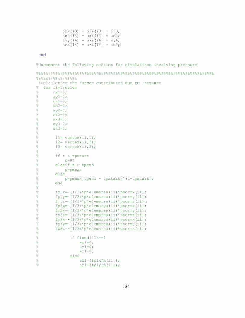
134

azz(i3) = azz(i3) + az3; axx(i4) = axx(i4) + ax4; ayy(i4) = ayy(i4) + ay4; azz(i4) = azz(i4) + az4; end %Uncomment the following section for simulations involving pressure %%%%%%%%%%%%%%%%%%%%%%%%%%%%%%%%%%%%%%%%%%%%%%%%%%%%%%%%%%%%%%%%%%%%%%%%%%%%%%%%%%%%%%%%%%% %Calculating the forces contributed due to Pressure % for ii=1:nelem % ax1=0; % ay1=0; % az1=0; % ax2=0; % ay2=0; % az2=0; % ax3=0; % ay3=0; % az3=0; % % i1= vertex(ii,1); % i2= vertex(ii,2); % i3= vertex(ii,3); % % if t < tpstart % p=0; % elseif t > tpend % p=pmax; % else % p=pmax/(tpend - tpstart)*(t-tpstart); % end % % fp1x=-(1/3)*p*elemarea(ii)*pnormx(ii); % fp1y=-(1/3)*p*elemarea(ii)*pnormy(ii); % fp1z=-(1/3)*p*elemarea(ii)*pnormz(ii); % fp2x=-(1/3)*p*elemarea(ii)*pnormx(ii); % fp2y=-(1/3)*p*elemarea(ii)*pnormy(ii); % fp2z=-(1/3)*p*elemarea(ii)*pnormz(ii); % fp3x=-(1/3)*p*elemarea(ii)*pnormx(ii); % fp3y=-(1/3)*p*elemarea(ii)*pnormy(ii); % fp3z=-(1/3)*p*elemarea(ii)*pnormz(ii); % % if fixed(i1)==1 % ax1=0; % ay1=0; % az1=0; % else % ax1=(fp1x/m(i1)); % ay1=(fp1y/m(i1));

135

% az1=(fp1z/m(i1)); % end % % if fixed(i2)==1 % ax2=0; % ay2=0; % az2=0; % else % ax2=(fp2x/m(i2)); % ay2=(fp2y/m(i2)); % az2=(fp2z/m(i2)); % end % % if fixed(i3)==1 % ax3=0; % ay3=0; % az3=0; % else % ax3=(fp3x/m(i3)); % ay3=(fp3y/m(i3)); % az3=(fp3z/m(i3)); % end % % axx(i1) = axx(i1) + ax1; % ayy(i1) = ayy(i1) + ay1; % azz(i1) = azz(i1) + az1; % axx(i2) = axx(i2) + ax2; % ayy(i2) = ayy(i2) + ay2; % azz(i2) = azz(i2) + az2; % axx(i3) = axx(i3) + ax3; % ayy(i3) = ayy(i3) + ay3; % azz(i3) = azz(i3) + az3; % % end %Accumulating forces on all structural vertices for ii=1:nnodes a(3*ii-2)=axx(ii); a(3*ii-1)=ayy(ii); a(3*ii) = azz(ii); aux1 = [v(6*ii-4); a(3*ii-2); v(6*ii-2); a(3*ii-1); v(6*ii); a(3*ii)]; dvdt = [dvdt; aux1]; end return

136

B Runge-Kutta Matlab Function Code

%Runge-Kutta Function to solve the Equations of Motion function [t,v]=RungeKutta_v2(t,v,h) dvdt = GridfunctBendTriangularRandom_v2(t, v); k1 = h*dvdt; dvdt = GridfunctBendTriangularRandom_v2(t+h/2, v+(k1')/2); k2 = h*dvdt; dvdt = GridfunctBendTriangularRandom_v2(t+h/2, v+(k2')/2); k3 = h*dvdt; dvdt = GridfunctBendTriangularRandom_v2(t+h, v+(k3')); k4 = h*dvdt; vaux = v' + (k1 + 2*k2 + 2*k3 + k4)/6; v=vaux'; return

137

C 11 x 11 Mesh Input File

121

1 0.1000000E+01 0.0000000E+00 0.0000000E+00 2 0.1000000E+01 0.1000000E+00 0.0000000E+00 3 0.9000000E+00 0.0000000E+00 0.0000000E+00 4 0.9000000E+00 0.1000000E+00 0.0000000E+00 5 0.1000000E+01 0.2000000E+00 0.0000000E+00 6 0.9000000E+00 0.2000000E+00 0.0000000E+00 7 0.1000000E+01 0.3000000E+00 0.0000000E+00 8 0.9000000E+00 0.3000000E+00 0.0000000E+00 9 0.1000000E+01 0.4000000E+00 0.0000000E+00 10 0.9000000E+00 0.4000000E+00 0.0000000E+00 11 0.1000000E+01 0.5000000E+00 0.0000000E+00 12 0.9000000E+00 0.5000000E+00 0.0000000E+00 13 0.1000000E+01 0.6000000E+00 0.0000000E+00 14 0.9000000E+00 0.6000000E+00 0.0000000E+00 15 0.1000000E+01 0.7000000E+00 0.0000000E+00 16 0.9000000E+00 0.7000000E+00 0.0000000E+00 17 0.1000000E+01 0.8000001E+00 0.0000000E+00 18 0.9000000E+00 0.8000001E+00 0.0000000E+00 19 0.1000000E+01 0.9000001E+00 0.0000000E+00 20 0.9000000E+00 0.9000001E+00 0.0000000E+00 21 0.1000000E+01 0.1000000E+01 0.0000000E+00 22 0.9000000E+00 0.1000000E+01 0.0000000E+00 23 0.8000000E+00 0.0000000E+00 0.0000000E+00 24 0.8000000E+00 0.9999999E-01 0.0000000E+00 25 0.8000000E+00 0.2000000E+00 0.0000000E+00 26 0.8000000E+00 0.3000000E+00 0.0000000E+00 27 0.8000000E+00 0.4000000E+00 0.0000000E+00 28 0.8000000E+00 0.5000000E+00 0.0000000E+00 29 0.8000000E+00 0.6000000E+00 0.0000000E+00 30 0.8000000E+00 0.7000000E+00 0.0000000E+00 31 0.8000000E+00 0.8000000E+00 0.0000000E+00 32 0.8000000E+00 0.9000001E+00 0.0000000E+00 33 0.8000000E+00 0.1000000E+01 0.0000000E+00 34 0.7000000E+00 0.0000000E+00 0.0000000E+00 35 0.7000000E+00 0.1000000E+00 0.0000000E+00 36 0.7000000E+00 0.2000000E+00 0.0000000E+00 37 0.7000000E+00 0.3000000E+00 0.0000000E+00 38 0.7000000E+00 0.4000000E+00 0.0000000E+00 39 0.7000000E+00 0.5000000E+00 0.0000000E+00 40 0.7000000E+00 0.6000000E+00 0.0000000E+00 41 0.7000000E+00 0.7000000E+00 0.0000000E+00 42 0.7000000E+00 0.8000001E+00 0.0000000E+00 43 0.7000000E+00 0.9000001E+00 0.0000000E+00

Total number of particles

x, y, z coordinate information

138

44 0.7000000E+00 0.1000000E+01 0.0000000E+00 45 0.6000000E+00 0.0000000E+00 0.0000000E+00 46 0.6000000E+00 0.1000000E+00 0.0000000E+00 47 0.6000000E+00 0.2000000E+00 0.0000000E+00 48 0.6000000E+00 0.3000000E+00 0.0000000E+00 49 0.6000000E+00 0.4000000E+00 0.0000000E+00 50 0.6000000E+00 0.5000000E+00 0.0000000E+00 51 0.6000000E+00 0.6000000E+00 0.0000000E+00 52 0.6000000E+00 0.7000000E+00 0.0000000E+00 53 0.6000000E+00 0.8000001E+00 0.0000000E+00 54 0.6000000E+00 0.9000001E+00 0.0000000E+00 55 0.6000000E+00 0.1000000E+01 0.0000000E+00 56 0.5000000E+00 0.0000000E+00 0.0000000E+00 57 0.5000000E+00 0.1000000E+00 0.0000000E+00 58 0.5000000E+00 0.2000000E+00 0.0000000E+00 59 0.5000000E+00 0.3000000E+00 0.0000000E+00 60 0.5000000E+00 0.4000000E+00 0.0000000E+00 61 0.5000000E+00 0.5000000E+00 0.0000000E+00 62 0.5000000E+00 0.6000000E+00 0.0000000E+00 63 0.5000000E+00 0.7000000E+00 0.0000000E+00 64 0.5000000E+00 0.8000001E+00 0.0000000E+00 65 0.5000000E+00 0.9000001E+00 0.0000000E+00 66 0.5000000E+00 0.1000000E+01 0.0000000E+00 67 0.4000000E+00 0.0000000E+00 0.0000000E+00 68 0.4000000E+00 0.1000000E+00 0.0000000E+00 69 0.4000000E+00 0.2000000E+00 0.0000000E+00 70 0.4000000E+00 0.3000000E+00 0.0000000E+00 71 0.4000000E+00 0.4000000E+00 0.0000000E+00 72 0.4000000E+00 0.5000000E+00 0.0000000E+00 73 0.4000000E+00 0.6000000E+00 0.0000000E+00 74 0.4000000E+00 0.7000000E+00 0.0000000E+00 75 0.4000000E+00 0.8000001E+00 0.0000000E+00 76 0.4000000E+00 0.9000001E+00 0.0000000E+00 77 0.4000000E+00 0.1000000E+01 0.0000000E+00 78 0.3000000E+00 0.0000000E+00 0.0000000E+00 79 0.3000000E+00 0.1000000E+00 0.0000000E+00 80 0.3000000E+00 0.2000000E+00 0.0000000E+00 81 0.3000000E+00 0.3000000E+00 0.0000000E+00 82 0.3000000E+00 0.4000000E+00 0.0000000E+00 83 0.3000000E+00 0.5000000E+00 0.0000000E+00 84 0.3000000E+00 0.6000000E+00 0.0000000E+00 85 0.3000000E+00 0.7000000E+00 0.0000000E+00 86 0.3000000E+00 0.8000001E+00 0.0000000E+00 87 0.3000000E+00 0.9000001E+00 0.0000000E+00 88 0.3000000E+00 0.1000000E+01 0.0000000E+00 89 0.1999999E+00 0.0000000E+00 0.0000000E+00 90 0.1999999E+00 0.9999999E-01 0.0000000E+00 91 0.1999999E+00 0.2000000E+00 0.0000000E+00 92 0.1999999E+00 0.3000000E+00 0.0000000E+00 93 0.1999999E+00 0.4000000E+00 0.0000000E+00 94 0.1999999E+00 0.5000000E+00 0.0000000E+00 95 0.1999999E+00 0.6000000E+00 0.0000000E+00 96 0.1999999E+00 0.7000000E+00 0.0000000E+00

x, y, z coordinate information continued

139

97 0.1999999E+00 0.8000001E+00 0.0000000E+00 98 0.1999999E+00 0.9000001E+00 0.0000000E+00 99 0.1999999E+00 0.1000000E+01 0.0000000E+00 100 0.9999990E-01 0.0000000E+00 0.0000000E+00 101 0.9999990E-01 0.1000000E+00 0.0000000E+00 102 0.9999990E-01 0.2000000E+00 0.0000000E+00 103 0.9999990E-01 0.3000000E+00 0.0000000E+00 104 0.9999990E-01 0.4000000E+00 0.0000000E+00 105 0.9999990E-01 0.5000000E+00 0.0000000E+00 106 0.9999990E-01 0.6000000E+00 0.0000000E+00 107 0.9999990E-01 0.7000000E+00 0.0000000E+00 108 0.9999990E-01 0.8000001E+00 0.0000000E+00 109 0.9999990E-01 0.9000001E+00 0.0000000E+00 110 0.9999990E-01 0.1000000E+01 0.0000000E+00 111 0.0000000E+00 0.0000000E+00 0.0000000E+00 112 0.0000000E+00 0.1000000E+00 0.0000000E+00 113 0.0000000E+00 0.2000000E+00 0.0000000E+00 114 0.0000000E+00 0.3000000E+00 0.0000000E+00 115 0.0000000E+00 0.4000000E+00 0.0000000E+00 116 0.0000000E+00 0.5000000E+00 0.0000000E+00 117 0.0000000E+00 0.6000000E+00 0.0000000E+00 118 0.0000000E+00 0.7000000E+00 0.0000000E+00 119 0.0000000E+00 0.8000001E+00 0.0000000E+00 120 0.0000000E+00 0.9000001E+00 0.0000000E+00 121 0.0000000E+00 0.1000000E+01 0.0000000E+00

1 2 2 3 2 4 1 3 4 5 3 4 1 2 4 23 4 6 2 3 5 6 23 24 5 4 2 4 6 7 6 6 4 5 7 8 24 25 7 4 5 6 8 9 8 6 6 7 9 10 25 26 9 4 7 8 10 11 10 6 8 9 11 12 26 27 11 4 9 10 12 13 12 6 10 11 13 14 27 28 13 4 11 12 14 15 14 6 12 13 15 16 28 29 15 4 13 14 16 17 16 6 14 15 17 18 29 30 17 4 15 16 18 19 18 6 16 17 19 20 30 31 19 4 17 18 20 21 20 6 18 19 21 22 31 32 21 3 19 20 22 22 4 20 21 32 33 23 4 3 4 24 34 24 6 4 6 23 25 34 35 25 6 6 8 24 26 35 36 26 6 8 10 25 27 36 37

nearest neighbor information for forces due to stretching

x, y, z coordinate information continued

140

27 6 10 12 26 28 37 38 28 6 12 14 27 29 38 39 29 6 14 16 28 30 39 40 30 6 16 18 29 31 40 41 31 6 18 20 30 32 41 42 32 6 20 22 31 33 42 43 33 4 22 32 43 44 34 4 23 24 35 45 35 6 24 25 34 36 45 46 36 6 25 26 35 37 46 47 37 6 26 27 36 38 47 48 38 6 27 28 37 39 48 49 39 6 28 29 38 40 49 50 40 6 29 30 39 41 50 51 41 6 30 31 40 42 51 52 42 6 31 32 41 43 52 53 43 6 32 33 42 44 53 54 44 4 33 43 54 55 45 4 34 35 46 56 46 6 35 36 45 47 56 57 47 6 36 37 46 48 57 58 48 6 37 38 47 49 58 59 49 6 38 39 48 50 59 60 50 6 39 40 49 51 60 61 51 6 40 41 50 52 61 62 52 6 41 42 51 53 62 63 53 6 42 43 52 54 63 64 54 6 43 44 53 55 64 65 55 4 44 54 65 66 56 4 45 46 57 67 57 6 46 47 56 58 67 68 58 6 47 48 57 59 68 69 59 6 48 49 58 60 69 70 60 6 49 50 59 61 70 71 61 6 50 51 60 62 71 72 62 6 51 52 61 63 72 73 63 6 52 53 62 64 73 74 64 6 53 54 63 65 74 75 65 6 54 55 64 66 75 76 66 4 55 65 76 77 67 4 56 57 68 78 68 6 57 58 67 69 78 79 69 6 58 59 68 70 79 80 70 6 59 60 69 71 80 81 71 6 60 61 70 72 81 82 72 6 61 62 71 73 82 83 73 6 62 63 72 74 83 84 74 6 63 64 73 75 84 85 75 6 64 65 74 76 85 86 76 6 65 66 75 77 86 87 77 4 66 76 87 88 78 4 67 68 79 89 79 6 68 69 78 80 89 90

nearest neighbor information for forces due to stretching continued

141

80 6 69 70 79 81 90 91 81 6 70 71 80 82 91 92 82 6 71 72 81 83 92 93 83 6 72 73 82 84 93 94 84 6 73 74 83 85 94 95 85 6 74 75 84 86 95 96 86 6 75 76 85 87 96 97 87 6 76 77 86 88 97 98 88 4 77 87 98 99 89 4 78 79 90 100 90 6 79 80 89 91 100 101 91 6 80 81 90 92 101 102 92 6 81 82 91 93 102 103 93 6 82 83 92 94 103 104 94 6 83 84 93 95 104 105 95 6 84 85 94 96 105 106 96 6 85 86 95 97 106 107 97 6 86 87 96 98 107 108 98 6 87 88 97 99 108 109 99 4 88 98 109 110 100 4 89 90 101 111 101 6 90 91 100 102 111 112 102 6 91 92 101 103 112 113 103 6 92 93 102 104 113 114 104 6 93 94 103 105 114 115 105 6 94 95 104 106 115 116 106 6 95 96 105 107 116 117 107 6 96 97 106 108 117 118 108 6 97 98 107 109 118 119 109 6 98 99 108 110 119 120 110 4 99 109 120 121 111 3 100 101 112 112 4 101 102 111 113 113 4 102 103 112 114 114 4 103 104 113 115 115 4 104 105 114 116 116 4 105 106 115 117 117 4 106 107 116 118 118 4 107 108 117 119 119 4 108 109 118 120 120 4 109 110 119 121 121 2 110 120 280 1 2 4 3 3 2 5 4 2 4 23 3 2 5 6 4 4 5 7 6 5 6 24 4 5 7 8 6

Total number of common edges for bending

connectivity information for forces resisting bending deformation

nearest neighbor information for forces due to stretching continued

142

7 8 25 6 6 7 9 8 7 9 10 8 8 9 11 10 9 10 26 8 9 11 12 10 10 11 13 12 11 12 27 10 11 13 14 12 13 14 28 12 12 13 15 14 13 15 16 14 14 15 17 16 15 16 29 14 15 17 18 16 16 17 19 18 17 18 30 16 17 19 20 18 19 20 31 18 18 19 21 20 19 21 22 20 21 22 32 20 3 4 24 23 4 24 34 23 23 4 6 24 4 6 25 24 24 6 8 25 6 25 35 24 6 8 26 25 25 8 10 26 8 26 36 25 8 10 27 26 10 27 37 26 26 10 12 27 10 12 28 27 27 12 14 28 12 28 38 27 12 14 29 28 28 14 16 29 14 29 39 28 14 16 30 29 16 30 40 29 29 16 18 30 16 18 31 30 30 18 20 31 18 31 41 30 18 20 32 31 31 20 22 32 20 32 42 31 20 22 33 32 22 33 43 32 23 24 35 34 34 24 25 35

connectivity information for forces resisting bending deformation continued

143

24 35 45 34 24 25 36 35 25 36 46 35 35 25 26 36 25 26 37 36 36 26 27 37 26 37 47 36 26 27 38 37 37 27 28 38 27 38 48 37 27 28 39 38 28 39 49 38 38 28 29 39 28 29 40 39 39 29 30 40 29 40 50 39 29 30 41 40 40 30 31 41 30 41 51 40 30 31 42 41 31 42 52 41 41 31 32 42 31 32 43 42 42 32 33 43 32 43 53 42 32 33 44 43 33 44 54 43 34 35 46 45 45 35 36 46 35 46 56 45 35 36 47 46 46 36 37 47 36 47 57 46 36 37 48 47 37 48 58 47 47 37 38 48 37 38 49 48 48 38 39 49 38 49 59 48 38 39 50 49 49 39 40 50 39 50 60 49 39 40 51 50 40 51 61 50 50 40 41 51 40 41 52 51 51 41 42 52 41 52 62 51 41 42 53 52 52 42 43 53 42 53 63 52 42 43 54 53 43 54 64 53


144

53 43 44 54 43 44 55 54 44 55 65 54 45 46 57 56 46 57 67 56 56 46 47 57 46 47 58 57 57 47 48 58 47 58 68 57 47 48 59 58 58 48 49 59 48 59 69 58 48 49 60 59 49 60 70 59 59 49 50 60 49 50 61 60 60 50 51 61 50 61 71 60 50 51 62 61 61 51 52 62 51 62 72 61 51 52 63 62 52 63 73 62 62 52 53 63 52 53 64 63 63 53 54 64 53 64 74 63 53 54 65 64 64 54 55 65 54 65 75 64 54 55 66 65 55 66 76 65 56 57 68 67 67 57 58 68 57 68 78 67 57 58 69 68 58 69 79 68 68 58 59 69 58 59 70 69 69 59 60 70 59 70 80 69 59 60 71 70 70 60 61 71 60 71 81 70 60 61 72 71 61 72 82 71 71 61 62 72 61 62 73 72 72 62 63 73 62 73 83 72 62 63 74 73 73 63 64 74 63 74 84 73


145

63 64 75 74 64 75 85 74 74 64 65 75 64 65 76 75 75 65 66 76 65 76 86 75 65 66 77 76 66 77 87 76 67 68 79 78 78 68 69 79 68 79 89 78 68 69 80 79 79 69 70 80 69 80 90 79 69 70 81 80 70 81 91 80 80 70 71 81 70 71 82 81 81 71 72 82 71 82 92 81 71 72 83 82 82 72 73 83 72 83 93 82 72 73 84 83 73 84 94 83 83 73 74 84 73 74 85 84 84 74 75 85 74 85 95 84 74 75 86 85 85 75 76 86 75 86 96 85 75 76 87 86 76 87 97 86 86 76 77 87 76 77 88 87 77 88 98 87 78 79 90 89 79 90 100 89 89 79 80 90 79 80 91 90 90 80 81 91 80 91 101 90 80 81 92 91 91 81 82 92 81 92 102 91 81 82 93 92 82 93 103 92 92 82 83 93 82 83 94 93 93 83 84 94 83 94 104 93 83 84 95 94


146

94 84 85 95 84 95 105 94 84 85 96 95 85 96 106 95 95 85 86 96 85 86 97 96 96 86 87 97 86 97 107 96 86 87 98 97 97 87 88 98 87 98 108 97 87 88 99 98 88 99 109 98 89 90 101 100 100 90 91 101 90 101 111 100 90 91 102 101 91 102 112 101 101 91 92 102 91 92 103 102 102 92 93 103 92 103 113 102 92 93 104 103 103 93 94 104 93 104 114 103 93 94 105 104 94 105 115 104 104 94 95 105 94 95 106 105 105 95 96 106 95 106 116 105 95 96 107 106 106 96 97 107 96 107 117 106 96 97 108 107 97 108 118 107 107 97 98 108 97 98 109 108 108 98 99 109 98 109 119 108 98 99 110 109 99 110 120 109 100 101 112 111 111 101 102 112 101 102 113 112 112 102 103 113 102 103 114 113 113 103 104 114 103 104 115 114 114 104 105 115 104 105 116 115 115 105 106 116 105 106 117 116


147

116 106 107 117 106 107 118 117 117 107 108 118 107 108 119 118 118 108 109 119 108 109 120 119 119 109 110 120 109 110 121 120 40

1 0.1000000E+01 0.0000000E+00 0.0000000E+00 2 0.1000000E+01 0.1000000E+00 0.0000000E+00 3 0.9000000E+00 0.0000000E+00 0.0000000E+00 5 0.1000000E+01 0.2000000E+00 0.0000000E+00 7 0.1000000E+01 0.3000000E+00 0.0000000E+00 9 0.1000000E+01 0.4000000E+00 0.0000000E+00 11 0.1000000E+01 0.5000000E+00 0.0000000E+00 13 0.1000000E+01 0.6000000E+00 0.0000000E+00 15 0.1000000E+01 0.7000000E+00 0.0000000E+00 17 0.1000000E+01 0.8000001E+00 0.0000000E+00 19 0.1000000E+01 0.9000001E+00 0.0000000E+00 21 0.1000000E+01 0.1000000E+01 0.0000000E+00 22 0.9000000E+00 0.1000000E+01 0.0000000E+00 23 0.8000000E+00 0.0000000E+00 0.0000000E+00 33 0.8000000E+00 0.1000000E+01 0.0000000E+00 34 0.7000000E+00 0.0000000E+00 0.0000000E+00 44 0.7000000E+00 0.1000000E+01 0.0000000E+00 45 0.6000000E+00 0.0000000E+00 0.0000000E+00 55 0.6000000E+00 0.1000000E+01 0.0000000E+00 56 0.5000000E+00 0.0000000E+00 0.0000000E+00 66 0.5000000E+00 0.1000000E+01 0.0000000E+00 67 0.4000000E+00 0.0000000E+00 0.0000000E+00 77 0.4000000E+00 0.1000000E+01 0.0000000E+00 78 0.3000000E+00 0.0000000E+00 0.0000000E+00 88 0.3000000E+00 0.1000000E+01 0.0000000E+00 89 0.1999999E+00 0.0000000E+00 0.0000000E+00 99 0.1999999E+00 0.1000000E+01 0.0000000E+00 100 0.9999990E-01 0.0000000E+00 0.0000000E+00 110 0.9999990E-01 0.1000000E+01 0.0000000E+00 111 0.0000000E+00 0.0000000E+00 0.0000000E+00 112 0.0000000E+00 0.1000000E+00 0.0000000E+00 113 0.0000000E+00 0.2000000E+00 0.0000000E+00 114 0.0000000E+00 0.3000000E+00 0.0000000E+00 115 0.0000000E+00 0.4000000E+00 0.0000000E+00 116 0.0000000E+00 0.5000000E+00 0.0000000E+00 117 0.0000000E+00 0.6000000E+00 0.0000000E+00 118 0.0000000E+00 0.7000000E+00 0.0000000E+00 119 0.0000000E+00 0.8000001E+00 0.0000000E+00 120 0.0000000E+00 0.9000001E+00 0.0000000E+00 121 0.0000000E+00 0.1000000E+01 0.0000000E+00

Total number of boundary nodes

boundary node coordinates


148

1 0 0 0

2 0 0 0 3 0 0 0 4 0 0 0 5 0 0 0 6 0 0 0 7 0 0 0 8 0 0 0 9 0 0 0 10 0 0 0 11 0 0 0 12 0 0 0 13 0 0 0 14 0 0 0 15 0 0 0 16 0 0 0 17 0 0 0 18 0 0 0 19 0 0 0 20 0 0 0 21 0 0 0 22 0 0 0 23 0 0 0 24 0 0 0 25 0 0 0 26 0 0 0 27 0 0 0 28 0 0 0 29 0 0 0 30 0 0 0 31 0 0 0 32 0 0 0 33 0 0 0 34 0 0 0 35 0 0 0 36 0 0 0 37 0 0 0 38 0 0 0 39 0 0 0 40 0 0 0 41 0 0 0 42 0 0 0 43 0 0 0 44 0 0 0 45 0 0 0 46 0 0 0 47 0 0 0 48 0 0 0 49 0 0 0 50 0 0 0 51 0 0 0 52 0 0 0

x, y, and z external forces for each particle

149

53 0 0 0 54 0 0 0 55 0 0 0 56 0 0 0 57 0 0 0 58 0 0 0 59 0 0 0 60 0 0 0 61 0 0 1 62 0 0 0 63 0 0 0 64 0 0 0 65 0 0 0 66 0 0 0 67 0 0 0 68 0 0 0 69 0 0 0 70 0 0 0 71 0 0 0 72 0 0 0 73 0 0 0 74 0 0 0 75 0 0 0 76 0 0 0 77 0 0 0 78 0 0 0 79 0 0 0 80 0 0 0 81 0 0 0 82 0 0 0 83 0 0 0 84 0 0 0 85 0 0 0 86 0 0 0 87 0 0 0 88 0 0 0 89 0 0 0 90 0 0 0 91 0 0 0 92 0 0 0 93 0 0 0 94 0 0 0 95 0 0 0 96 0 0 0 97 0 0 0 98 0 0 0 99 0 0 0 100 0 0 0 101 0 0 0 102 0 0 0 103 0 0 0 104 0 0 0 105 0 0 0

x, y, and z external forces for each particle continued

150

106 0 0 0 107 0 0 0 108 0 0 0 109 0 0 0 110 0 0 0 111 0 0 0 112 0 0 0 113 0 0 0 114 0 0 0 115 0 0 0 116 0 0 0 117 0 0 0 118 0 0 0 119 0 0 0 120 0 0 0 121 0 0 0

1 1 2 1 3 1 4 0 5 1 6 0 7 1 8 0 9 1 10 0 11 1 12 0 13 1 14 0 15 1 16 0 17 1 18 0 19 1 20 0 21 1 22 1 23 1 24 0 25 0 26 0 27 0 28 0 29 0 30 0 31 0 32 0 33 1 34 1 35 0

free (0) or simply supported (1) boundary conditions for each particle

x, y, and z external forces for each particle continued

151

36 0 37 0 38 0 39 0 40 0 41 0 42 0 43 0 44 1 45 1 46 0 47 0 48 0 49 0 50 0 51 0 52 0 53 0 54 0 55 1 56 1 57 0 58 0 59 0 60 0 61 0 62 0 63 0 64 0 65 0 66 1 67 1 68 0 69 0 70 0 71 0 72 0 73 0 74 0 75 0 76 0 77 1 78 1 79 0 80 0 81 0 82 0 83 0 84 0 85 0 86 0 87 0 88 1

free (0) or simply supported (1) boundary conditions for each particle continued

152

89 1 90 0 91 0 92 0 93 0 94 0 95 0 96 0 97 0 98 0 99 1 100 1 101 0 102 0 103 0 104 0 105 0 106 0 107 0 108 0 109 0 110 1 111 1 112 1 113 1 114 1 115 1 116 1 117 1 118 1 119 1 120 1 121 1 200 1 1 2 3 2 3 2 4 3 4 2 5 4 5 6 4 5 7 6 5 6 8 6 7 7 7 9 8 8 8 9 10 9 10 9 11 10 11 12 10 11 13 12 11 12 14 12 13 13 13 15 14 14 14 15 16 15 16 15 17

Total number of elements

element connectivity information for all of the elements

free (0) or simply supported (1) boundary conditions for each particle continued

153

16 17 18 16 17 19 18 17 18 20 18 19 19 19 21 20 20 20 21 22 21 4 23 3 22 24 23 4 23 4 6 24 24 24 6 25 25 25 6 8 26 8 26 25 27 10 26 8 28 27 26 10 29 10 12 27 30 27 12 28 31 28 12 14 32 14 29 28 33 16 29 14 34 30 29 16 35 16 18 30 36 30 18 31 37 31 18 20 38 20 32 31 39 22 32 20 40 33 32 22 41 34 23 24 42 24 35 34 43 25 35 24 44 36 35 25 45 25 26 36 46 36 26 37 47 37 26 27 48 27 38 37 49 28 38 27 50 39 38 28 51 28 29 39 52 39 29 40 53 40 29 30 54 30 41 40 55 31 41 30 56 42 41 31 57 31 32 42 58 42 32 43 59 43 32 33 60 33 44 43 61 34 35 45 62 45 35 46 63 46 35 36 64 36 47 46 65 37 47 36 66 48 47 37 67 37 38 48 68 48 38 49

element connectivity information for all of the elements continued

154

69 49 38 39 70 39 50 49 71 40 50 39 72 51 50 40 73 40 41 51 74 51 41 52 75 52 41 42 76 42 53 52 77 43 53 42 78 54 53 43 79 43 44 54 80 54 44 55 81 46 56 45 82 57 56 46 83 46 47 57 84 57 47 58 85 58 47 48 86 48 59 58 87 49 59 48 88 60 59 49 89 49 50 60 90 60 50 61 91 61 50 51 92 51 62 61 93 52 62 51 94 63 62 52 95 52 53 63 96 63 53 64 97 64 53 54 98 54 65 64 99 55 65 54 100 66 65 55 101 67 56 57 102 57 68 67 103 58 68 57 104 69 68 58 105 58 59 69 106 69 59 70 107 70 59 60 108 60 71 70 109 61 71 60 110 72 71 61 111 61 62 72 112 72 62 73 113 73 62 63 114 63 74 73 115 64 74 63 116 75 74 64 117 64 65 75 118 75 65 76 119 76 65 66 120 66 77 76 121 67 68 78


155

122 78 68 79 123 79 68 69 124 69 80 79 125 70 80 69 126 81 80 70 127 70 71 81 128 81 71 82 129 82 71 72 130 72 83 82 131 73 83 72 132 84 83 73 133 73 74 84 134 84 74 85 135 85 74 75 136 75 86 85 137 76 86 75 138 87 86 76 139 76 77 87 140 87 77 88 141 79 89 78 142 90 89 79 143 79 80 90 144 90 80 91 145 91 80 81 146 81 92 91 147 82 92 81 148 93 92 82 149 82 83 93 150 93 83 94 151 94 83 84 152 84 95 94 153 85 95 84 154 96 95 85 155 85 86 96 156 96 86 97 157 97 86 87 158 87 98 97 159 88 98 87 160 99 98 88 161 100 89 90 162 90 101 100 163 91 101 90 164 102 101 91 165 91 92 102 166 102 92 103 167 103 92 93 168 93 104 103 169 94 104 93 170 105 104 94 171 94 95 105 172 105 95 106 173 106 95 96 174 96 107 106


156

175 97 107 96 176 108 107 97 177 97 98 108 178 108 98 109 179 109 98 99 180 99 110 109 181 100 101 111 182 111 101 112 183 112 101 102 184 102 113 112 185 103 113 102 186 114 113 103 187 103 104 114 188 114 104 115 189 115 104 105 190 105 116 115 191 106 116 105 192 117 116 106 193 106 107 117 194 117 107 118 195 118 107 108 196 108 119 118 197 109 119 108 198 120 119 109 199 109 110 120 200 120 110 121


157

D Cantilever Bending Test Spreadsheet Results

Report for: College of Textiles North Carolina State University, Physical Testing Lab Date of Report: 12/9/2009 ASTM D1388-Stiffness of Fabrics Worksheet for Raw Data Sample Identification: Canvas Material

Bending Length

(C) Flexural Rigidity

(G) Specimen Overhang Lengths (o) c=0/2 G=W x c^3 Number units=cm (Report to nearest 0.1 cm) units=cm units=mg.cm

Warp (Machine) Filling (Cross) Warp Filling W F Specimen 1 8.1 8.5

8.7 9.3 8.3 8.4 8.6 9.3

Specimen 1 Average 8.4 8.9 4.2 4.4 2824.6 3301.8 Specimen 2 9.1 9.1

9.1 9.7 8.5 8.5 8.6 9.1


8.7 10.0 8.5 8.6 8.9 10.1


8.5 10.2 8.0 8.7 8.6 9.5

Specimen 4 Average 8.5 9.5 4.3 4.7 2900.7 4017.7 TOTAL AVERAGE 8.6 9.2 4.3 4.6 3027.2 3724.1

ASTM D3776-Mass per Unit Area (Weight) of Woven Fabric (Needed to calculate flexural rigidity.) (Weigh all 8 1" x 8" specimens before measuring stiffness.)

Total Wt. in Grams: 15.60 0.0026 0.0032 Total Area in sq. inches: 64.00 *Flexural Rigidity in units lb-in Fabric mass/area (mg/cm^2): 37.79 Fabric mass/area (oz/yd^2): 11.14

158

E Case 1 Main Matlab Code

clc clear all %Declaring variables used in both functions as global global d0 nnodes m c k0 kb fxext fyext fzext fixed coords NNM bend nconnect kap0 nelem vertex pmax tpstart tpend gx gy gz a %Defining the input parameters t=0; %initial time tfinal = 10; %final time h = 0.0004; %time-step N=tfinal/h; %total number of steps hstl=250; %number of steps between STL files mperarea=0.0024; %mass per unit area k0=21.828; %stretching stiffness coefficient input in the code kb=.0000054; %bending stiffness coefficient c= 0.0005; %damping coefficient pmax=0.0; %maximum pressure tpstart=0; %time at which pressure force begins tpend=0; %time at which pressure force = pmax gx=0.0; %acceleration due to gravity in the x-direction gy=-32.174; %acceleration due to gravity in the y-direction gz=0; %acceleration due to gravity in the z-direction neglimit = -0.5; %negative limit for box method poslimit = 3.0; %positive limit for box method contactcheckelem = []; distcheck = 1.5; %radius for the distance check method soldiertlag = 0.1; %time the impactor begins moving boostlimit = 40; %limit on the adjustable parameter b boostmax=0; boostcounter=0; vimpact1=0.4; %velocity of the impactor plotcounter=0; stlcount=1; %Open, read, and close the text file for the tent geometry fid = fopen('hextentbendstifftune_refined.txt', 'r'); nnodes = fscanf(fid, '%d',1); for i=1:nnodes nnum=fscanf(fid, '%d',1); for j=1:3 coords(nnum,j)=fscanf(fid, '%f', 1); end

159

end for i=1:nnodes nnum=fscanf(fid, '%d',1); nneighbors=fscanf(fid,'%d',1); NNM(i,1)=nnum; NNM(i,2)=nneighbors; for j=1:nneighbors NNM(nnum,j+2)=fscanf(fid,'%d',1); end end nconnect=fscanf(fid,'%d',1); for i=1:nconnect for j=1:4 bend(i,j)=fscanf(fid, '%d', 1); end end npossiblebc=fscanf(fid, '%d', 1); fixed(1:nnodes) = 0; for i=1:npossiblebc nnum=fscanf(fid, '%d', 1); for j=1:3 fixdummy=fscanf(fid, '%f', 1); end end force = zeros(nnodes,3); for i=1:nnodes nnum=fscanf(fid, '%d', 1); for j=1:3 force(nnum,j)=fscanf(fid, '%f', 1); end end %Only use this if going to leave the fixed part in the input file for i=1:nnodes nnum=fscanf(fid, '%d', 1); fixed(nnum)=fscanf(fid, '%d', 1); end nelem=fscanf(fid, '%d', 1); for i=1:nelem nnum=fscanf(fid, '%d', 1); for j=1:3 vertex(nnum,j)=fscanf(fid, '%d', 1); end end fclose(fid);

160

%Open, read, close text file for the impactor fid = fopen('single impactor point.txt', 'r'); nnodes1 = fscanf(fid, '%d',1); coords1=zeros(nnodes1,3); for i=1:nnodes1 nnum=fscanf(fid, '%d',1); for j=1:3 coords1(nnum,j)=fscanf(fid, '%f', 1); end end nelem1=fscanf(fid, '%d', 1); vertex1=zeros(nnodes1,3); for i=1:nelem1 nnum=fscanf(fid, '%d', 1); for j=1:3 vertex1(nnum,j)=fscanf(fid, '%d', 1); end end fclose(fid); m = zeros(1,nnodes); %Loop to assign the mass to each particle based on element area %Also define the range of elements which are checked for contact for ii=1:nelem m1=0; m2=0; m3=0; i1= vertex(ii,1); i2= vertex(ii,2); i3= vertex(ii,3); Ax=coords(i1,1); Ay=coords(i1,2); Az=coords(i1,3); Bx=coords(i2,1); By=coords(i2,2); Bz=coords(i2,3); Cx=coords(i3,1); Cy=coords(i3,2); Cz=coords(i3,3); %Assigning possible contact elements based on the box method limits if (neglimit < Ay && Ay < poslimit) && (neglimit < By && By <

poslimit) && (neglimit < Cy && Cy < poslimit) contactcheckelem = [contactcheckelem; ii]; end

161

v1=sqrt((Bx-Ax)^2+(By-Ay)^2+(Bz-Az)^2); v1x=(Bx-Ax); v1y=(By-Ay); v1z=(Bz-Az); v2=sqrt((Cx-Ax)^2+(Cy-Ay)^2+(Cz-Az)^2); v2x=(Cx-Ax); v2y=(Cy-Ay); v2z=(Cz-Az); pnorm=sqrt((v1y*v2z-v1z*v2y)^2+(v1z*v2x-v1x*v2z)^2+(v1x*v2y-

v1y*v2x)^2); elemarea=1/2*pnorm; m1=(1/3)*mperarea*elemarea; m2=(1/3)*mperarea*elemarea; m3=(1/3)*mperarea*elemarea; m(i1)= m(i1) + m1; m(i2)= m(i2) + m2; m(i3)= m(i3) + m3; end %If the initial surface is curved, need to define an initial kappa %Need to loop over the number of connections, just like in gridfunct, %Calculate kap0, may have to do some checks incase kap>90 or so for hh=1:nconnect i1= bend(hh,1); i2= bend(hh,2); i3= bend(hh,3); i4= bend(hh,4); L=(1/2)*sqrt((coords(i1,1)-coords(i3,1))^2 + (coords(i1,2)-

coords(i3,2))^2 + (coords(i1,3)-coords(i3,3))^2); x1=coords(i1,1); y1=coords(i1,2); z1=coords(i1,3); x2=coords(i2,1); y2=coords(i2,2); z2=coords(i2,3); x3=coords(i3,1); y3=coords(i3,2); z3=coords(i3,3); x4=coords(i4,1);

162

y4=coords(i4,2); z4=coords(i4,3); t12=sqrt((x2-x1)^2 + (y2-y1)^2 + (z2-z1)^2); t12x=(x2-x1)/t12; t12y=(y2-y1)/t12; t12z=(z2-z1)/t12; t14=sqrt((x4-x1)^2 + (y4-y1)^2 + (z4-z1)^2); t14x=(x4-x1)/t14; t14y=(y4-y1)/t14; t14z=(z4-z1)/t14; t12xt14=sqrt((t12y*t14z-t12z*t14y)^2 + (t12z*t14x-t12x*t14z)^2

+ (t12x*t14y-t12y*t14x)^2); n124x=(t12y*t14z-t12z*t14y)/t12xt14; n124y=(t12z*t14x-t12x*t14z)/t12xt14; n124z=(t12x*t14y-t12y*t14x)/t12xt14; t23=sqrt((x3-x2)^2 + (y3-y2)^2 + (z3-z2)^2); t23x=(x3-x2)/t23; t23y=(y3-y2)/t23; t23z=(z3-z2)/t23; t24=sqrt((x4-x2)^2 + (y4-y2)^2 + (z4-z2)^2); t24x=(x4-x2)/t24; t24y=(y4-y2)/t24; t24z=(z4-z2)/t24; t23xt24=sqrt((t23y*t24z-t23z*t24y)^2 + (t23z*t24x-t23x*t24z)^2

+ (t23x*t24y-t23y*t24x)^2); n234x=(t23y*t24z-t23z*t24y)/t23xt24; n234y=(t23z*t24x-t23x*t24z)/t23xt24; n234z=(t23x*t24y-t23y*t24x)/t23xt24; navg=sqrt(((n124x+n234x)/2)^2 +((n124y+n234y)/2)^2 +

((n124z+n234z)/2)^2); n24x=((n124x+n234x)/2)/navg; n24y=((n124y+n234y)/2)/navg; n24z=((n124z+n234z)/2)/navg; dot=(n124x*n234x + n124y*n234y + n124z*n234z); if dot > 1 dot=1; end

163

dphi=acos(dot); t12dotn234=(t12x*n234x + t12y*n234y + t12z*n234z); dphi=-sign(t12dotn234)*dphi; kap0(hh)=dphi/L; end %%%%Preallocation of variables ximpactinit=zeros(1,nnodes1); yimpactinit=zeros(1,nnodes1); zimpactinit=zeros(1,nnodes1); contact=zeros(1,nnodes1); preimpactdotsign=zeros(1,nnodes1); ximpact=zeros(1,nnodes1); yimpact=zeros(1,nnodes1); zimpact=zeros(1,nnodes1); vximpact=zeros(1,nnodes1); vyimpact=zeros(1,nnodes1); vzimpact=zeros(1,nnodes1); Px=zeros(1,nnodes1); Py=zeros(1,nnodes1); Pz=zeros(1,nnodes1); centroidx=zeros(1,nnodes1); centroidy=zeros(1,nnodes1); centroidz=zeros(1,nnodes1); Pcent=zeros(1,nnodes1); v1=zeros(1,nnodes1); v1x=zeros(1,nnodes1); v1y=zeros(1,nnodes1); v1z=zeros(1,nnodes1); v2=zeros(1,nnodes1); v2x=zeros(1,nnodes1); v2y=zeros(1,nnodes1); v2z=zeros(1,nnodes1); v3=zeros(1,nnodes1); v3x=zeros(1,nnodes1); v3y=zeros(1,nnodes1); v3z=zeros(1,nnodes1); pnorm=zeros(1,nnodes1); pnormx=zeros(1,nnodes1); pnormy=zeros(1,nnodes1); pnormz=zeros(1,nnodes1); vAP=zeros(1,nnodes1); vAPx=zeros(1,nnodes1); vAPy=zeros(1,nnodes1); vAPz=zeros(1,nnodes1); ndotvAP=zeros(1,nnodes1); Qx=zeros(1,nnodes1); Qy=zeros(1,nnodes1); Qz=zeros(1,nnodes1);

164

AQ=zeros(1,nnodes1); AQx=zeros(1,nnodes1); AQy=zeros(1,nnodes1); AQz=zeros(1,nnodes1); BQ=zeros(1,nnodes1); BQx=zeros(1,nnodes1); BQy=zeros(1,nnodes1); BQz=zeros(1,nnodes1); CQ=zeros(1,nnodes1); CQx=zeros(1,nnodes1); CQy=zeros(1,nnodes1); CQz=zeros(1,nnodes1); elemarea=zeros(1,nnodes1); area1=zeros(1,nnodes1); area2=zeros(1,nnodes1); area3=zeros(1,nnodes1); areatotal=zeros(1,nnodes1); contactelem=zeros(1,nnodes1); x=zeros(1,nnodes1); y=zeros(1,nnodes1); z=zeros(1,nnodes1); QPx=zeros(1,nnodes1); QPy=zeros(1,nnodes1); QPz=zeros(1,nnodes1); maxdistnode=zeros(1,length(contactcheckelem)); maxdist=zeros(1,length(contactcheckelem)); %Assigning external force values from input text file for s=1:nnodes fxext(s)=force(s,1); fyext(s)=force(s,2); fzext(s)=force(s,3); end vel = zeros(1,3*nnodes); v0 = zeros(1,6*nnodes); %for loop to store initial conditions of the mesh for r=1:nnodes aux = [coords(r,1) vel(3*r-2) coords(r,2) vel(3*r-1) coords(r,3) vel(3*r)]; v0(1,6*r-5:6*r) = aux; end %Command when using the Runge-Kutta ODE Solver v=v0; vvector=v0; tvector=t; penetrate=0; %For loop to store initial conditions of the impactor for i=1:nnodes1

165

ximpactinit(i)=coords1(i,1); yimpactinit(i)=coords1(i,2); zimpactinit(i)=coords1(i,3); end count=0; numimpact=nnodes1; %Creating STL file for Initial Conditions fOut = sprintf('SingleImpactor.%d.stl',1); fid = fopen(fOut, 'wt'); fprintf(fid,'solid object \n'); for i=1:nelem n1 = vertex(i,1); n2 = vertex(i,2); n3 = vertex(i,3); fprintf(fid,' facet normal %f %f %f\n',1.0,0.0,0.0); fprintf(fid,' outer loop \n'); vertx1 = vvector(1,6*n1-5); verty1 = vvector(1,6*n1-3); vertz1 = vvector(1,6*n1-1); vertx2 = vvector(1,6*n2-5); verty2 = vvector(1,6*n2-3); vertz2 = vvector(1,6*n2-1); vertx3 = vvector(1,6*n3-5); verty3 = vvector(1,6*n3-3); vertz3 = vvector(1,6*n3-1); fprintf(fid, ' vertex %f %f %f\n',vertx1,verty1,vertz1); fprintf(fid, ' vertex %f %f %f\n',vertx2,verty2,vertz2); fprintf(fid, ' vertex %f %f %f\n',vertx3,verty3,vertz3); fprintf(fid,' endloop \n'); fprintf(fid,' endfacet \n'); end for i=1:nelem1 fprintf(fid,' facet normal %f %f %f\n',1.0,0.0,0.0); fprintf(fid,' outer loop \n'); fprintf(fid, ' vertex %f %f %f \n'

,ximpactinit(vertex1(i,1)),yimpactinit(vertex1(i,1)),zimpactinit(vertex1(i,1)));

fprintf(fid, ' vertex %f %f %f\n' ,ximpactinit(vertex1(i,2)),yimpactinit(vertex1(i,2)),zimpactinit(vertex1(i,2)));

fprintf(fid, ' vertex %f %f %f\n' ,ximpactinit(vertex1(i,3)),yimpactinit(vertex1(i,3)),zimpactinit(vertex1(i,3)));

fprintf(fid,' endloop \n'); fprintf(fid,' endfacet \n'); end

166

fprintf(fid,'endsolid object'); fclose(fid); %Where the code actually begins, call Runge-Kutta function for i=1:N [t,v]=RungeKutta_v2(t,v,h); for k=1:numimpact if t < soldiertlag ximpact(k)=ximpactinit(k); yimpact(k)=yimpactinit(k); zimpact(k)=zimpactinit(k); vximpact(k)=0; vyimpact(k)=0; vzimpact(k)=0; else ximpact(k)=ximpactinit(k); yimpact(k)=yimpactinit(k); zimpact(k)=zimpactinit(k)-vimpact1*(t-soldiertlag); vximpact(k)=0; vyimpact(k)=0; vzimpact(k)=-vimpact1; end end maxpen=0; maxdistnode=zeros(1,length(contactcheckelem)); maxdist=zeros(1,length(contactcheckelem)); if t == soldiertlag || t > soldiertlag %Embedded for loops, k over the impactors, j over the possible contact %elements for k=1:numimpact for j=1:length(contactcheckelem) Ax(k)=v(6*vertex(contactcheckelem(j),1)-5); Ay(k)=v(6*vertex(contactcheckelem(j),1)-3); Az(k)=v(6*vertex(contactcheckelem(j),1)-1); Bx(k)=v(6*vertex(contactcheckelem(j),2)-5); By(k)=v(6*vertex(contactcheckelem(j),2)-3); Bz(k)=v(6*vertex(contactcheckelem(j),2)-1); Cx(k)=v(6*vertex(contactcheckelem(j),3)-5); Cy(k)=v(6*vertex(contactcheckelem(j),3)-3); Cz(k)=v(6*vertex(contactcheckelem(j),3)-1); Px(k)=ximpact(k);

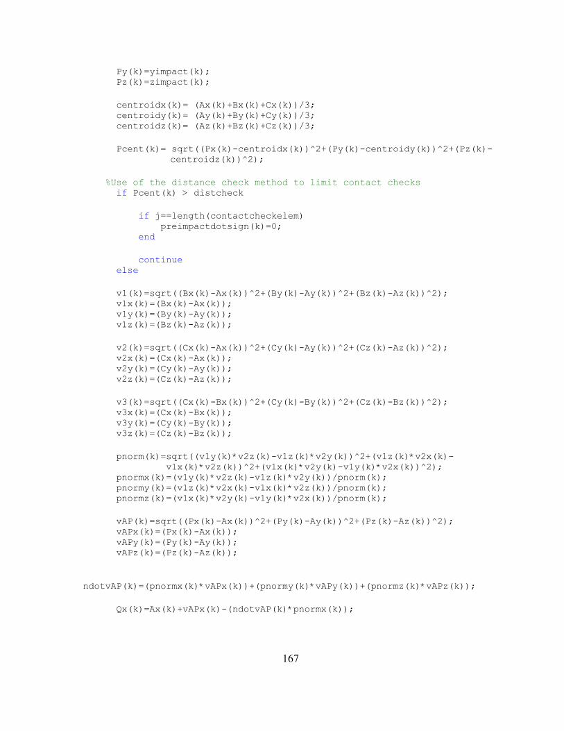
167

Py(k)=yimpact(k); Pz(k)=zimpact(k); centroidx(k)= (Ax(k)+Bx(k)+Cx(k))/3; centroidy(k)= (Ay(k)+By(k)+Cy(k))/3; centroidz(k)= (Az(k)+Bz(k)+Cz(k))/3; Pcent(k)= sqrt((Px(k)-centroidx(k))^2+(Py(k)-centroidy(k))^2+(Pz(k)-

centroidz(k))^2); %Use of the distance check method to limit contact checks if Pcent(k) > distcheck if j==length(contactcheckelem) preimpactdotsign(k)=0; end continue else v1(k)=sqrt((Bx(k)-Ax(k))^2+(By(k)-Ay(k))^2+(Bz(k)-Az(k))^2); v1x(k)=(Bx(k)-Ax(k)); v1y(k)=(By(k)-Ay(k)); v1z(k)=(Bz(k)-Az(k)); v2(k)=sqrt((Cx(k)-Ax(k))^2+(Cy(k)-Ay(k))^2+(Cz(k)-Az(k))^2); v2x(k)=(Cx(k)-Ax(k)); v2y(k)=(Cy(k)-Ay(k)); v2z(k)=(Cz(k)-Az(k)); v3(k)=sqrt((Cx(k)-Bx(k))^2+(Cy(k)-By(k))^2+(Cz(k)-Bz(k))^2); v3x(k)=(Cx(k)-Bx(k)); v3y(k)=(Cy(k)-By(k)); v3z(k)=(Cz(k)-Bz(k)); pnorm(k)=sqrt((v1y(k)*v2z(k)-v1z(k)*v2y(k))^2+(v1z(k)*v2x(k)-

v1x(k)*v2z(k))^2+(v1x(k)*v2y(k)-v1y(k)*v2x(k))^2); pnormx(k)=(v1y(k)*v2z(k)-v1z(k)*v2y(k))/pnorm(k); pnormy(k)=(v1z(k)*v2x(k)-v1x(k)*v2z(k))/pnorm(k); pnormz(k)=(v1x(k)*v2y(k)-v1y(k)*v2x(k))/pnorm(k); vAP(k)=sqrt((Px(k)-Ax(k))^2+(Py(k)-Ay(k))^2+(Pz(k)-Az(k))^2); vAPx(k)=(Px(k)-Ax(k)); vAPy(k)=(Py(k)-Ay(k)); vAPz(k)=(Pz(k)-Az(k)); ndotvAP(k)=(pnormx(k)*vAPx(k))+(pnormy(k)*vAPy(k))+(pnormz(k)*vAPz(k)); Qx(k)=Ax(k)+vAPx(k)-(ndotvAP(k)*pnormx(k));

168

Qy(k)=Ay(k)+vAPy(k)-(ndotvAP(k)*pnormy(k)); Qz(k)=Az(k)+vAPz(k)-(ndotvAP(k)*pnormz(k)); AQ(k)=sqrt((Qx(k)-Ax(k))^2+(Qy(k)-Ay(k))^2+(Qz(k)-Az(k))^2); AQx(k)=(Qx(k)-Ax(k)); AQy(k)=(Qy(k)-Ay(k)); AQz(k)=(Qz(k)-Az(k)); BQ(k)=sqrt((Qx(k)-Bx(k))^2+(Qy(k)-By(k))^2+(Qz(k)-Bz(k))^2); BQx(k)=(Qx(k)-Bx(k)); BQy(k)=(Qy(k)-By(k)); BQz(k)=(Qz(k)-Bz(k)); CQ(k)=sqrt((Qx(k)-Cx(k))^2+(Qy(k)-Cy(k))^2+(Qz(k)-Cz(k))^2); CQx(k)=(Qx(k)-Cx(k)); CQy(k)=(Qy(k)-Cy(k)); CQz(k)=(Qz(k)-Cz(k)); elemarea(k)=1/2*pnorm(k); area1(k)=1/2*sqrt((v1y(k)*AQz(k)-v1z(k)*AQy(k))^2+(v1z(k)*AQx(k)-

v1x(k)*AQz(k))^2+(v1x(k)*AQy(k)-v1y(k)*AQx(k))^2); area2(k)=1/2*sqrt((AQy(k)*v2z(k)-AQz(k)*v2y(k))^2+(AQz(k)*v2x(k)-

AQx(k)*v2z(k))^2+(AQx(k)*v2y(k)-AQy(k)*v2x(k))^2); area3(k)=1/2*sqrt((v3y(k)*BQz(k)-v3z(k)*BQy(k))^2+(v3z(k)*BQx(k)-

v3x(k)*BQz(k))^2+(v3x(k)*BQy(k)-v3y(k)*BQx(k))^2); areatotal(k)=area1(k)+area2(k)+area3(k); if areatotal(k) > elemarea(k) + 0.0001 &&

j==length(contactcheckelem) preimpactdotsign(k) = 0; break elseif areatotal(k) > elemarea(k) + 0.0001 continue else contactelem(k)=contactcheckelem(j); %put this back up here QP=sqrt((Px(k)-Qx(k))^2+(Py(k)-Qy(k))^2+(Pz(k)-Qz(k))^2); QPx(k)=(Px(k)-Qx(k)); QPy(k)=(Py(k)-Qy(k)); QPz(k)=(Pz(k)-Qz(k)); normdotQPtrial=(pnormx(k)*QPx(k))+(pnormy(k)*QPy(k))+(pnormz(k)*QPz(k)); trialsign=sign(normdotQPtrial); end if i > 1 if preimpactdotsign(k) == 0 preimpactdotsign(k) = trialsign; break elseif trialsign == preimpactdotsign(k) break else if maxdistnode(j) == 0

169

maxdistnode(j)=k; maxdist(j) = QP; break elseif QP < maxdist(j) break else maxdistnode(j)=k; maxdist(j) = QP; break end end end end end end %Loop over the possible contact elements for j = 1:length(contactcheckelem) if maxdistnode(j)==0 continue end k = maxdistnode(j); vdotnorm=(vximpact(k)*pnormx(k))+(vyimpact(k)*pnormy(k))+(vzimpact(k)*pnor mz(k)); vnormalx=vdotnorm*pnormx(k); vnormaly=vdotnorm*pnormy(k); vnormalz=vdotnorm*pnormz(k); if maxdist(j) > maxpen maxpen = maxdist(j); end contact(k)=contact(k)+1; boostaux = (maxdist(j)/(abs(vdotnorm)*h))+1; if boostaux < boostlimit boost = boostaux; else boost = boostlimit; boostcounter=boostcounter+1; end

170

if boost > boostmax boostmax = boost; end %Updating the velocities of the contact element vertices v(6*vertex(contactelem(k),1)-4) = boost*vnormalx; v(6*vertex(contactelem(k),1)-2) = boost*vnormaly; v(6*vertex(contactelem(k),1)) = boost*vnormalz; v(6*vertex(contactelem(k),2)-4) = boost*vnormalx; v(6*vertex(contactelem(k),2)-2) = boost*vnormaly; v(6*vertex(contactelem(k),2)) = boost*vnormalz; v(6*vertex(contactelem(k),3)-4) = boost*vnormalx; v(6*vertex(contactelem(k),3)-2) = boost*vnormaly; v(6*vertex(contactelem(k),3)) = boost*vnormalz; end end plotcounter=plotcounter+1; t=t+h if plotcounter==hstl vvector=[vvector; v]; tvector=[tvector; t]; penetrate=[penetrate; maxpen]; stlcount=stlcount+1; %Creating STL files while the code is running instead of waiting until it %completes for k=1:numimpact x(k)=ximpact(k); y(k)=yimpact(k); z(k)=zimpact(k); end fOut = sprintf('SingleImpactor.%d.stl',stlcount); fid = fopen(fOut, 'wt'); fprintf(fid,'solid object \n'); for ii=1:nelem n1 = vertex(ii,1); n2 = vertex(ii,2); n3 = vertex(ii,3); fprintf(fid,' facet normal %f %f %f\n',1.0,0.0,0.0); fprintf(fid,' outer loop \n'); vertx1 = vvector(stlcount,6*n1-5); verty1 = vvector(stlcount,6*n1-3); vertz1 = vvector(stlcount,6*n1-1); vertx2 = vvector(stlcount,6*n2-5);

171

verty2 = vvector(stlcount,6*n2-3); vertz2 = vvector(stlcount,6*n2-1); vertx3 = vvector(stlcount,6*n3-5); verty3 = vvector(stlcount,6*n3-3); vertz3 = vvector(stlcount,6*n3-1); fprintf(fid, ' vertex %f %f %f\n'

,vertx1,verty1,vertz1); fprintf(fid, ' vertex %f %f %f\n'

,vertx2,verty2,vertz2); fprintf(fid, ' vertex %f %f %f\n'

,vertx3,verty3,vertz3); fprintf(fid,' endloop \n'); fprintf(fid,' endfacet \n'); end for ii=1:nelem1 fprintf(fid,' facet normal %f %f %f\n',1.0,0.0,0.0); fprintf(fid,' outer loop \n'); fprintf(fid, ' vertex %f %f %f\n'

,x(vertex1(ii,1)),y(vertex1(ii,1)),z(vertex1(ii,1))); fprintf(fid, ' vertex %f %f %f\n'

,x(vertex1(ii,2)),y(vertex1(ii,2)),z(vertex1(ii,2))); fprintf(fid, ' vertex %f %f %f\n'

,x(vertex1(ii,3)),y(vertex1(ii,3)),z(vertex1(ii,3))); fprintf(fid,' endloop \n'); fprintf(fid,' endfacet \n'); end fprintf(fid,'endsolid object'); fclose(fid); plotcounter=0; end end %Plot statement to show maximum penetration vs. time figure(1),plot(tvector,penetrate); %Plot statement to show x,y,and z positions and velocities for the given %particles figure(265),plot(tvector,vvector(:,1585),'b-',tvector,vvector(:,1586),'b--',tvector,vvector(:,1587),'r-',tvector,vvector(:,1588),'r--',tvector,vvector(:,1589),'g-',tvector,vvector(:,1590),'g--'); figure(276),plot(tvector,vvector(:,1651),'b-',tvector,vvector(:,1652),'b--',tvector,vvector(:,1653),'r-',tvector,vvector(:,1654),'r--',tvector,vvector(:,1655),'g-',tvector,vvector(:,1656),'g--');

172

F Case 2 Main Matlab Code (Input Parameters Only)

%Defining the input parameters t=0; %initial time tfinal = 12; %final time h = 0.0004; %time-step N=tfinal/h; %total number of steps hstl=300; %number of steps between STL files mperarea=0.0024; %mass per unit area k0=21.828; %stretching stiffness coefficient input in the code kb=.0000054; %bending stiffness coefficient c= 0.0005; %damping coefficient pmax=0.0; %maximum pressure tpstart=0; %time at which pressure force begins tpend=0; %time at which pressure force = pmax gx=0.0; %acceleration due to gravity in the x-direction gy=-32.174; %acceleration due to gravity in the y-direction gz=0.0; %acceleration due to gravity in the z-direction neglimit = -0.5; %negative limit for box method poslimit = 1.8; %positive limit for box method contactcheckelem = []; distcheck = 1.5; %radius for the distance check method soldiertlag = 0.1; %time the impactor begins moving boostlimit = 40; %limit on the adjustable parameter b boostmax=0; boostcounter=0; vimpact1=0.55; %velocity of impactor 1 vimpact2=0.5; %velocity of impactor 2 vimpact3=0.4; %velocity of impactor 3 vimpact4=0.3; %velocity of impactor 4 vimpact5=0.1; %velocity of impactor 5

173

G Case 2 Multiple Impactor Sample Input File

15

1 0.0950000E+01 0.0000000E+01 0.0600000E+01 2 0.0800000E+01 0.0300000E+01 0.0600000E+01 3 0.0650000E+01 0.0000000E+01 0.0600000E+01 4 0.4920000E+01 0.0100000E+01 0.0600000E+01 5 0.4770000E+01 0.0400000E+01 0.0600000E+01 6 0.4620000E+01 0.0100000E+01 0.0600000E+01 7 0.2350000E+01 0.0700000E+01 0.0700000E+01 8 0.2200000E+01 0.1000000E+01 0.0700000E+01 9 0.2050000E+01 0.0700000E+01 0.0700000E+01 10 0.3750000E+01 0.0550000E+01 0.0700000E+01 11 0.3600000E+01 0.0850000E+01 0.0700000E+01 12 0.3450000E+01 0.0550000E+01 0.0700000E+01 13 0.3066500E+01 0.0650000E+01 0.0800000E+01 14 0.2916500E+01 0.0950000E+01 0.0800000E+01 15 0.2766500E+01 0.0650000E+01 0.0800000E+01

5

1 1 2 3 2 4 5 6 3 7 8 9 4 10 11 12 5 13 14 15

Total number of elements

Total number of particles

x, y, and z coordinate information for each particle

element connectivity information for each element

174

H Case 3 Main Matlab Code (Input Parameters Only)

%Defining the input parameters t=0; %initial time tfinal = 8; %final time h = 0.0004; %time-step N=tfinal/h; %total number of steps hstl=200; %number of steps between STL files mperarea=0.0024; %mass per unit area k0=21.828; %stretching stiffness coefficient input in the code kb=.0000054; %bending stiffness coefficient c= 0.0005; %damping coefficient pmax=0.0; %maximum pressure tpstart=0; %time at which pressure force begins tpend=0; %time at which pressure force = pmax gx=0.0; %acceleration due to gravity in the x-direction gy=-32.174; %acceleration due to gravity in the y-direction gz=0.0; %acceleration due to gravity in the z-direction neglimit = -0.5; %negative limit for box method poslimit = 1.0; %positive limit for box method contactcheckelem = []; distcheck = 1.2; %radius for the distance check method soldiertlag = 0.1; %time the impactor begins moving boostlimit = 75; %limit on the adjustable parameter b boostmax=0; boostcounter=0; vimpact1=0.8; %velocity of the impactor in the -x-direction vimpact2=0.24; %velocity of the impactor in the -z-direction

175

I Case 4 Main Matlab Code (Input Parameters Only)

%Defining the input parameters t=0; %initial time tfinal = 10; %final time h = 0.0002; %time-step N=tfinal/h; %total number of steps hstl=500; %number of steps between STL files mperarea=0.0024; %mass per unit area k0=21.828; %stretching stiffness coefficient input in code kb=.0000054; %bending stiffness coefficient c= 0.0005; %damping coefficient pmax=0.0; %max pressure tpstart=0; %time at which pressure begins tpend=0; %time at which pressure = pmax gx=0.0; %acceleration due to gravity in the x-direction gy=0.0; %acceleration due to gravity in the y-direction gz=0.0; %acceleration due to gravity in the z-direction neglimit = -0.4; %negative limit for the box method poslimit = 0.4; %positive limit for the box method contactcheckelem = []; distcheck = 0.7; %radius for the distance check method soldiertlag = 0.1; %time the impactor begins moving boostlimit = 75; %limit on the adjustable parameter b boostmax=0; boostcounter=0; vimpact1=0.5; %velocity of the impactor

176

J Case 5 Main Matlab Code (Input Parameters Only)

%Defining the input parameters t=0; %initial time tfinal = 10; %final time h = 0.0002; %time-step N=tfinal/h; %total number of steps hstl=500; %number of steps between STL files mperarea=0.0024; %mass per unit area k0=21.828; %stretching stiffness coefficient input in code kb=.0000054; %bending stiffness coefficient c= 0.0005; %damping coefficient pmax=0.0; %max pressure tpstart=0; %time at which pressure begins tpend=0; %time at which pressure = pmax gx=0.0; %acceleration due to gravity in the x-direction gy=0.0; %acceleration due to gravity in the y-direction gz=-32.174; %acceleration due to gravity in the z-direction neglimit = -0.96; %negative limit for box method poslimit = 1.02; %positive limit for box method contactcheckelem = []; distcheck = 0.7; %radius for the distance check method soldiertlag = 2.6; %time the impactor begins moving boostlimit = 75; %limit on the adjustable parameter b boostmax=0; boostcounter=0; vimpact1=0.8; %velocity of the impactor

177

K Case 6 Main Matlab Code (Input Parameters Only)

%Defining the input parameters t=0; %initial time tfinal = 12; %final time h = 0.00015; %time-step N=tfinal/h; %total number of steps hstl=800; %number of steps between STL files mperarea=0.0024; %mass per unit area k0=21.828; %stretching stiffness coefficient input in code kb=.0000054; %bending stiffness coefficient c= 0.0005; %damping coefficient pmax=0.15; %max pressure tpstart=2.6; %time at which pressure begins tpend=4.6; %time at which pressure = pmax gx=0.0; %acceleration due to gravity in the x-direction gy=0.0; %acceleration due to gravity in the y-direction gz=-32.174; %acceleration due to gravity in the z-direction neglimit = -0.96; %negative limit for box method poslimit = 1.02; %positive limit for box method contactcheckelem = []; distcheck = 0.7; %radius for the distance check method soldiertlag = 4.6; %time the impactor begins moving boostlimit = 75; %limit on the adjustable parameter b boostmax=0; boostcounter=0; fixstretch=0.75; %distance nodes are stretched during first time-

step vimpact1=0.8; %velocity of the impactor

178

L Case 7 Main Matlab Code (Input Parameters Only)

%Defining the input parameters t=0; %initial time tfinal = 16; %final time h = 0.000125; %time-step N=tfinal/h; %total number of steps hstl=1280; %number of steps between STL files mperarea=0.0024; %mass per unit area k0=21.828; %stretching stiffness coefficient input in code kb=.0000054; %bending stiffness coefficient c= 0.0005; %damping coefficient pmax=0.0; %max pressure tpstart=0; %time at which pressure begins tpend=0; %time at which pressure = pmax gx=0.0; %acceleration due to gravity in the x-direction gy=0.0; %acceleration due to gravity in the y-direction gz=-32.174; %acceleration due to gravity in the z-direction neglimit = -0.96; %negative limit for the box method poslimit = 1.02; %positive limit for the box method contactcheckelem = []; distcheck = 0.7; %radius for the distance check method soldiertlag = 2.0; %time the impactor begins moving boostlimit = 75; %limit on the adjustable parameter boostmax=0; boostcounter=0; vimpact1=0.8; %velocity of the impactor

flexible structure impact modeling with a particle method - nathan donald obringer

Documents

external forces

effective forces

internal forces

particle method

bend forces

gravitational forces

plane membrane forces

absolute damping forces