flexible learning approach to physics êêê · pdf fileflap p5.5 the...
TRANSCRIPT
F L E X I B L E L E A R N I N G A P P R O A C H T O P H Y S I C S
FLAP P5.5 The mathematics of oscillationsCOPYRIGHT © 1998 THE OPEN UNIVERSITY S570 V1.1
Module P5.5 The mathematics of oscillations1 Opening items
1.1 Module introduction
1.2 Fast track questions
1.3 Ready to study?
2 Oscillations and differential equations
2.1 Introducing mechanical and electrical oscillations
2.2 Mathematical models of mechanical and electricaloscillators
2.3 Second order differential equations1—1a brief review
2.4 Harmonic oscillations: simple, damped and driven
2.5 Electrical impedance
2.6 Mechanical impedance
2.7 Resonance and driven oscillations
3 Oscillations and complex numbers
3.1 Complex numbers1—1a brief review
3.2 Complex impedance
3.3 The power dissipated
4 Superposed oscillations and complex algebra
4.1 Superposition of two SHMs differing only in phase constant
4.2 Superposition of two SHMs differing in angular frequency and phase constant
4.3 Superposition of many SHMs—the diffraction grating
5 Closing items
5.1 Module summary
5.2 Achievements
5.3 Exit test
Exit module
FLAP P5.5 The mathematics of oscillationsCOPYRIGHT © 1998 THE OPEN UNIVERSITY S570 V1.1
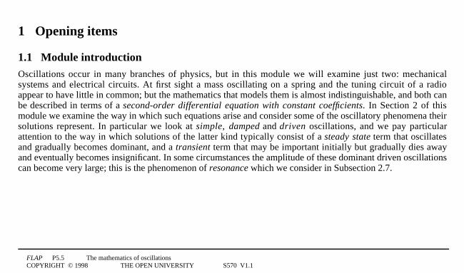
1 Opening items
1.1 Module introductionOscillations occur in many branches of physics, but in this module we will examine just two: mechanicalsystems and electrical circuits. At first sight a mass oscillating on a spring and the tuning circuit of a radioappear to have little in common; but the mathematics that models them is almost indistinguishable, and both canbe described in terms of a second-order differential equation with constant coefficients. In Section 2 of thismodule we examine the way in which such equations arise and consider some of the oscillatory phenomena theirsolutions represent. In particular we look at simple, damped and driven oscillations, and we pay particularattention to the way in which solutions of the latter kind typically consist of a steady state term that oscillatesand gradually becomes dominant, and a transient term that may be important initially but gradually dies awayand eventually becomes insignificant. In some circumstances the amplitude of these dominant driven oscillationscan become very large; this is the phenomenon of resonance which we consider in Subsection 2.7.
FLAP P5.5 The mathematics of oscillationsCOPYRIGHT © 1998 THE OPEN UNIVERSITY S570 V1.1
Very often it is only the steady state behaviour of the system that is of interest, and we may then assume that thetransient term is zero. In such cases we are able to abandon the differential equation approach, and use a muchsimpler method based on complex numbers. This technique is particularly relevant to the analysis of alternatingcurrents in electrical circuits, and in Section 3 we use it to develop a complex version of Ohm’s law. We will seethat the current and the applied voltage oscillate at the same rate, but they do not necessarily do so in phase dueto the complex impedance of the circuit concerned. In Subsection 3.3 we use complex methods to calculate thepower dissipated in an electrical circuit, and in the final section we examine how complex numbers may be usedto combine simple harmonic motions.
Study comment Having read the introduction you may feel that you are already familiar with the material covered by thismodule and that you do not need to study it. If so, try the Fast track questions given in Subsection 1.2. If not, proceeddirectly to Ready to study? in Subsection 1.3.

FLAP P5.5 The mathematics of oscillationsCOPYRIGHT © 1998 THE OPEN UNIVERSITY S570 V1.1
1.2 Fast track questions
Study comment Can you answer the following Fast track questions?. If you answer the questions successfully you needonly glance through the module before looking at the Module summary (Subsection 5.1) and the Achievements listed inSubsection 5.2. If you are sure that you can meet each of these achievements, try the Exit test in Subsection 5.3. If you havedifficulty with only one or two of the questions you should follow the guidance given in the answers and read the relevantparts of the module. However, if you have difficulty with more than two of the Exit questions you are strongly advised tostudy the whole module.
Question F1
Write down the differential equation for the current I(t) in a circuit containing a resistance R, a capacitance Cand an inductance L in series, that is driven by an applied voltage V01sin1(Ω1t). What is the general form of thesteady state solution to this equation?
FLAP P5.5 The mathematics of oscillationsCOPYRIGHT © 1998 THE OPEN UNIVERSITY S570 V1.1
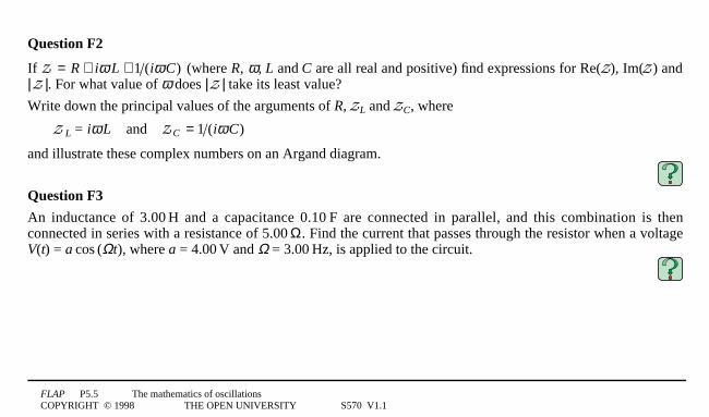
Question F2
If Z = R + iω L + 1 (iω C) (where R, ω, L and C are all real and positive) find expressions for Re(Z), Im(Z) and|1Z1|. For what value of ω does |1Z1| take its least value?
Write down the principal values of the arguments of R, ZL and ZC, where
Z1L = iω1L4and4 ZC = 1 (iω C)
and illustrate these complex numbers on an Argand diagram.
Question F3
An inductance of 3.001H and a capacitance 0.101F are connected in parallel, and this combination is thenconnected in series with a resistance of 5.001Ω. Find the current that passes through the resistor when a voltageV(t) = a1cos1(Ωt), where a = 4.001V and Ω = 3.001Hz, is applied to the circuit.
FLAP P5.5 The mathematics of oscillationsCOPYRIGHT © 1998 THE OPEN UNIVERSITY S570 V1.1
Study comment Having seen the Fast track questions you may feel that it would be wiser to follow the normal routethrough the module and to proceed directly to Ready to study? in Subsection 1.3.
Alternatively, you may still be sufficiently comfortable with the material covered by the module to proceed directly to theClosing items.

FLAP P5.5 The mathematics of oscillationsCOPYRIGHT © 1998 THE OPEN UNIVERSITY S570 V1.1
1.3 Ready to study?
Study comment This module is intended to form a link between the maths and physics strands of FLAP. It therefore makesmuch heavier mathematical demands than most modules, though it assumes less knowledge of physics. To begin the study ofthis module you will need to be familiar with the solution of second-order differential equations with constant coefficients(though we provide a brief review of this topic in Subsection 2.3), and you should also know how such equations arise fromNewton’s second law of motion. You should be able to manipulate trigonometric identities. You should also be familiar withthe Cartesian coordinate system, complex numbers, including their exponential representation (z = reiθ), the Argand diagramand the real part, imaginary part, modulus argument and complex conjugate of a complex number (although we provide youwith a short summary of the subject in Subsection 3.1). You should also be able to differentiate and integrate standardfunctions such as sin1(x0), cos1(x0) and exp1(x0). A familiarity with geometric progressions would also be useful, although notessential. It would be helpful if you have seen how oscillatory systems arise in physics, but we assume no prior knowledge inthis area. If you are unfamiliar with any of these topics you can review them by referring to the Glossary, which will indicatewhere in FLAP they are developed. The following Ready to study questions will help you to establish whether you need toreview some of the above topics before embarking on this module.

FLAP P5.5 The mathematics of oscillationsCOPYRIGHT © 1998 THE OPEN UNIVERSITY S570 V1.1
Question R1
Sketch the graph of y = 31sin1(ω1t + δ1) for
(a) ω = 21s−1 and δ = 0, (b) ω = 21s−1 and δ = −π/2.
How would the first graph you drew change if
(c) ω = 21s−1 and δ = −4, (d) ω = 21s−1 and δ = 4.
(e) Describe (without drawing a diagram) the graph of y = sin1(ω1t + π/2).
Question R2
Calculate the value of φ given that
cos φ = 2
22 + 32 and sin φ = −3
22 + 32
Use the trigonometric identity cos(A + B) = cos A cos B − sin Asin B to express 2 1cos1(ω1t) + 31sin1(ω1t) in theform R1cos1(ω1t + φ).

FLAP P5.5 The mathematics of oscillationsCOPYRIGHT © 1998 THE OPEN UNIVERSITY S570 V1.1
Question R3
Solve the quadratic equation h2 + 5h + 6 = 0.
Question R4
If z is defined by z = 4e5i1π0/04, what are the principal values of arg(z), |1z1|, Re(z) and Im(z)?
If you are unsure about any of these terms consult complex numbers in the Glossary.
Question R5
(Optional) What is the sum of the geometric series
1 + r + r02 + r3 + … + r1n−1
What is the sum for the particular case of r = i (where i12 = −1) and n = 9?

FLAP P5.5 The mathematics of oscillationsCOPYRIGHT © 1998 THE OPEN UNIVERSITY S570 V1.1
E
x0
D
x0
C
x0
B
x0
A
x0
mtim
e
Figure 14The vibrationsof a mechanical system.
2 Oscillations and differential equations
2.1 Introducing mechanical and electrical oscillationsFigure 1 shows a small body of mass m held between two stretched springs on asmooth horizontal table. Under the influence of the springs, the body is able to moveto and fro along a line that we will take to be the x-axis of a system of Cartesiancoordinates.
The equilibrium position of the body will be taken to be the point x = 0, so theposition coordinate of the body at any time t determines its displacement fromequilibrium at that time.
If the body is released from rest at a point slightly to the right of its equilibriumposition at some initial time t = 0 (diagram A), it will subsequently oscillate back andforth about its equilibrium position, as indicated in diagrams B, C, D and E.
As a result, the instantaneous position of the body will be a function of time and canbe denoted by x(t). The dashed line in Figure 1 is a graphical representation of thisfunction, although it would be more natural for us to draw the graph of x(t) with the t-axis horizontal and the x-axis vertical,
FLAP P5.5 The mathematics of oscillationsCOPYRIGHT © 1998 THE OPEN UNIVERSITY S570 V1.1
x(t)
t
amplitudeE
D
C
B
A
(a)
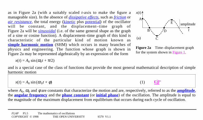
Figure 2a4Time–displacement graphfor the system shown in Figure 1.
as in Figure 2a (with a suitably scaled t-axis to make the figure amanageable size). In the absence of dissipative effects, such as friction orair resistance, the total energy (kinetic plus potential) of the oscillatorwill be constant, and the displacement–time graph ofFigure 2a will be sinusoidal (i.e. of the same general shape as the graphof a sine or cosine function). A displacement–time graph of this kind ischaracteristic of the particular kind of motion known assimple harmonic motion (SHM) which occurs in many branches ofphysics and engineering. The function whose graph is shown inFigure 2a may be represented algebraically by an expression of the form
x(t) = A01sin1(ω0t + π/2)
and is a special case of the class of functions that provide the most general mathematical description of simpleharmonic motion
x(t) = A01sin1(ω000t + φ) (1)
where A0, ω0 and φ are constants that characterize the motion and are, respectively, referred to as the amplitude,the angular frequency and the phase constant (or initial phase) of the oscillation. The amplitude is equal tothe magnitude of the maximum displacement from equilibrium that occurs during each cycle of oscillation.

FLAP P5.5 The mathematics of oscillationsCOPYRIGHT © 1998 THE OPEN UNIVERSITY S570 V1.1
The angular frequency is related to the period T (i.e. the time required for one complete oscillation such as thatfrom A to E in Figure 1) and to the frequency f by the relation
ω0 = 2π/T = 2πf
Thus the frequency (1f = 1/T) is the number of oscillations per second, and the angular frequency is just 2π timesthat value. The phase constant determines the value of x at t = 0, since x(0) = A01sin1(φ). Note that the alternativename for φ, the initial phase, arises because the quantity (ω0t + φ) which determines the stage that the oscillatorhas reached in its cycle at any time t is called the phase, and φ is simply the value of the phase at t = 0.

FLAP P5.5 The mathematics of oscillationsCOPYRIGHT © 1998 THE OPEN UNIVERSITY S570 V1.1
a difference in phasex(t)
t
(b)t0
Figure 2b4Effect of varying theiniyial phase on the time–displacement graph for the systemshown in Figure 1.
Figure 2b shows the effect of changing the initial phase of an oscillator. Theequation describing the dashed line was given above asx(t) = A01sin1(ω0t + π/2), so it corresponds to a phase constant φ = π/2. Thismay be contrasted with the equation describing the solid curve, which maybe written
x(t) = A1sin1(ω1t + π/2 − ω0t0)
and which corresponds to a phase constant φ = π/2 − ω0t0. The quantity t0indicates the extent to which the behaviour of the oscillator represented bythe solid curve lags behind that represented by the dashed curve. We cantherefore say that there is a phase difference between the two oscillators, andthat the former (represented by the solid curve) lags the latter (represented bythe dashed curve) by ω0t0.

FLAP P5.5 The mathematics of oscillationsCOPYRIGHT © 1998 THE OPEN UNIVERSITY S570 V1.1
decreasingamplitude
x(t)
t
(c)
A
B D
C
E
Figure 2c4Effect of damping on thetime–displacement graph for the systemshown in Figure 1.
In practice, an oscillating system of the kind shown in Figure 1 would besubject to friction and other dissipative effects and would lose energy toits environment. As a result of this energy transfer, the maximumdisplacement attained during each oscillation generally tends to decreasewith time, resulting in the sort of damped oscillations indicated inFigure 2c. Provided the damping is sufficiently light it is possible todescribe this kind of oscillation in a similar way to the simple harmonicoscillation described above. Of course, the description is not exactly thesame; the damping generally tends to reduce the angular frequency fromω0 to some lower value ω, and causes the amplitude to become a(decreasing) function of time A(t), but apart from these changes we canoften describe the damped oscillations by a function of the form
x(t) = A(t)1sin1(ω1t + φ) (2)

FLAP P5.5 The mathematics of oscillationsCOPYRIGHT © 1998 THE OPEN UNIVERSITY S570 V1.1
m
xrough surface
P
(a)
Figure 3a4A mass subject torestoring, damping and drivingforces.
Now consider the system shown in Figure 3a, in which a body of mass m isattached to one end of a horizontal spring, the other end of which is attachedto a fixed point P. The body can slide back and forth along a straight line,which we will again take to be the x-axis, but this time it is subject to anexternally imposed force (acting along the x-axis) in addition to the force dueto the spring and any dissipative force that may act. In this situation theexternally imposed force is called a driving force and the oscillations that ithelps to produce and sustain in the oscillator are called forced or drivenoscillations. If the driving force varies sinusoidally with time, at angularfrequency Ω , so that it may be described by an expression of the formF01sin1(Ω1t), we will eventually find that the motion of the oscillating bodyunder the influence of the driving force is described by
x(t) = A1sin1(Ω1t − δ1) (3)
where A and δ are constants whose values depend on the angular frequency of the driving force, Ω, and thecharacteristics of the oscillator, but are independent of time. The steady nature of the eventual motion shows thatin this case work done by the driving force is somehow compensating the oscillator for the energy it loses due todissipative effects.
What physical interpretation can you give to the parameters A and δ that appear in Equation 3?

FLAP P5.5 The mathematics of oscillationsCOPYRIGHT © 1998 THE OPEN UNIVERSITY S570 V1.1
Oscillations, whether simple, damped or driven are not confined to mechanical systems. All sorts of physicalsystems exhibit oscillations. Temperatures may oscillate from day to day or season to season; concentrations ofdifferent chemicals may rise and fall in oscillating chemical reactions; electric charges may oscillate back andforth in appropriately constructed electrical circuits; and so on. The properties of electrical oscillations areparticularly important and provide interesting analogies with mechanical oscillations. We will now brieflydescribe some of the situations in which electrical oscillations arise, and then investigate the reasons why suchapparently different systems should exhibit such closely similar behaviour.

FLAP P5.5 The mathematics of oscillationsCOPYRIGHT © 1998 THE OPEN UNIVERSITY S570 V1.1
R
~
C
(b)
V(t)
L
VC(t)VR(t)
I(t)
VL(t)
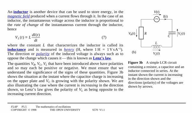
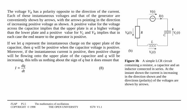
Figure 3b4A simple LCR circuitcontaining a resistor, a capacitor and aninductor connected in series. At theinstant shown the current is increasingin the direction shown and thedirections (polarity) of the voltages areshown by arrows.
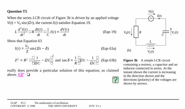
An electric circuit is a closed path around which electric charge mayflow. A typical circuit, such as that of Figure 3b, contains a number ofelectrical components that assist or retard the flow of charge and therebygive the circuit its particular characteristics. In order for the flow ofcharge to occur at all there must generally be a potential differencebetween one part of the circuit and another; this is measured in volts (V,where 11V = 11J1C−1) and is often referred to as a voltage. It might besupplied by a battery, but in the case of Figure 3b there is avoltage generator, shown by the symbol at the top of the diagram, whichproduces a time dependent potential difference V(t) between its terminals.The instantaneous rate of flow of charge at any point in the circuitconstitutes the instantaneous current I(t) at that point, and may bemeasured in amperes (A, where 11A = 11C1s−1). The conventional currentdirection is taken to be that of positive charge flow. The rest of the circuitshown in Figure 3b consists of a resistor (shown as the rectangle), acapacitor (shown as parallel bars) and an inductor (shown as the coil),connected in series, so that the same current flows through eachcomponent. Such circuits are called series LCR circuits.
FLAP P5.5 The mathematics of oscillationsCOPYRIGHT © 1998 THE OPEN UNIVERSITY S570 V1.1
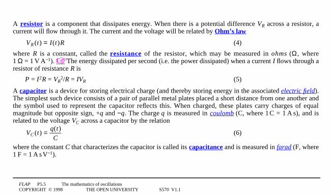
A resistor is a component that dissipates energy. When there is a potential difference VR across a resistor, acurrent will flow through it. The current and the voltage will be related by Ohm’s law
VR (t) = I(t)R (4)
where R is a constant, called the resistance of the resistor, which may be measured in ohms (Ω, where11Ω = 11V1A−1). The energy dissipated per second (i.e. the power dissipated) when a current I flows through aresistor of resistance R is
P = I02R = VR2/R = IVR (5)
A capacitor is a device for storing electrical charge (and thereby storing energy in the associated electric field).The simplest such device consists of a pair of parallel metal plates placed a short distance from one another andthe symbol used to represent the capacitor reflects this. When charged, these plates carry charges of equalmagnitude but opposite sign, +q and −q. The charge q is measured in coulomb (C, where 11C = 11A1s), and isrelated to the voltage VC across a capacitor by the relation
VC (t) = q(t)C
(6)
where the constant C that characterizes the capacitor is called its capacitance and is measured in farad (F, where11F = 11A1s1V−1).
FLAP P5.5 The mathematics of oscillationsCOPYRIGHT © 1998 THE OPEN UNIVERSITY S570 V1.1
R
~
C
(b)
V(t)
L
VC(t)VR(t)
I(t)
VL(t)
Figure 3b4A simple LCR circuitcontaining a resistor, a capacitor and aninductor connected in series. At theinstant shown the current is increasingin the direction shown and thedirections (polarity) of the voltages areshown by arrows.
An inductor is another device that can be used to store energy, in themagnetic field produced when a current flows through it. In the case of aninductor, the instantaneous voltage across the inductor is proportional tothe rate of change of the instantaneous current through the inductor,hence
VL (t) = LdI(t)
dt(7)
where the constant L that characterizes the inductor is called itsinductance and is measured in henry (H, where 11H = 11V1s1A−1).The direction or polarity of the induced voltage is always such as tooppose the change which causes it1—1this is known as Lenz’s law.
The quantities VR, VC, VL that have been introduced above have polaritiesand so may each be positive or negative. We must ensure that weunderstand the significance of the signs of these quantities. Figure 3bshows the situation at the instant where the capacitor charge is increasingon the upper plate and VC is growing with the polarity shown. We arealso illustrating the case where the current is increasing in the directionshown, so Lenz’s law gives the polarity of VL as being opposite to theincreasing current direction.
FLAP P5.5 The mathematics of oscillationsCOPYRIGHT © 1998 THE OPEN UNIVERSITY S570 V1.1
R
~
C
(b)
V(t)
L
VC(t)VR(t)
I(t)
VL(t)
Figure 3b4A simple LCR circuitcontaining a resistor, a capacitor and aninductor connected in series. At theinstant shown the current is increasingin the direction shown and thedirections (polarity) of the voltages areshown by arrows.
The voltage VR has a polarity opposite to the direction of the current.Each of these instantaneous voltages and that of the generator areconveniently shown by arrows, with the arrows pointing in the directionof increasing positive voltage as shown. A positive value for the voltageacross the capacitor implies that the upper plate is at a higher voltagethan the lower plate and a positive value for VL and VR implies that ineach case the end nearer to the generator is positive.
If we let q represent the instantaneous charge on the upper plate of thecapacitor, then q will be positive when the capacitor voltage is positive.Moreover, if the instantaneous current is positive, then positive chargewill be flowing onto the upper plate of the capacitor and q will beincreasing, this tells us nothing about the sign of q but it does ensure that
I = dq
dt(8)

FLAP P5.5 The mathematics of oscillationsCOPYRIGHT © 1998 THE OPEN UNIVERSITY S570 V1.1
R
~
C
(b)
V(t)
L
VC(t)VR(t)
I(t)
m
xrough surface
P
(a)
VL(t)
As you can see from the above discussion, the circuit shown inFigure 3b will be characterized by the relevant values of R, C and L.Given these three values and the specific form of the externally suppliedvoltage V(t), it is possible to determine the current I(t) that flows throughthe circuit, and the associated charge q(t) on the upper plate of thecapacitor. Interestingly the circuit turns out to be an electrical analogueof the driven mechanical oscillator shown in Figure 3a. In particular, ifthe external voltage is of the form V(t) = V01sin1(Ω1t), then eventually,after any transient currents have died away:
q(t) = A1sin1(Ω1t − δ1) (9)
and, consequently I(t) = dq
dt= AΩ cos(Ω t − δ ) (10)
Figure 34(a) A mass subject to restoring, damping and driving forces.(b) A simple LCR circuit containing a resistor, a capacitor and an inductorconnected in series. At the instant shown the current is increasing in the directionshown and the directions (polarity) of the voltages are shown by arrows.
FLAP P5.5 The mathematics of oscillationsCOPYRIGHT © 1998 THE OPEN UNIVERSITY S570 V1.1
If you compare Equation 9 with Equation 3
q(t) = A1sin1(Ω1t − δ1) (Eqn 9)
x(t) = A1sin1(Ω1t − δ1) (Eqn 3)
you will see that they are both of the same form. It is in this sense that the charge oscillations in the series LCRcircuit driven by an externally supplied sinusoidal voltage may be said to be analogous to the displacementoscillations of the mechanical oscillator driven by an externally supplied sinusoidal force.
In the next subsection you will see why these two very different physical systems give rise to essentiallyidentical oscillatory phenomena. The essential point is that the underlying physics of both systems is describedby very similar equations.
FLAP P5.5 The mathematics of oscillationsCOPYRIGHT © 1998 THE OPEN UNIVERSITY S570 V1.1
2.2 Mathematical models of mechanical and electrical oscillators
m
xrough surface
P
(a)
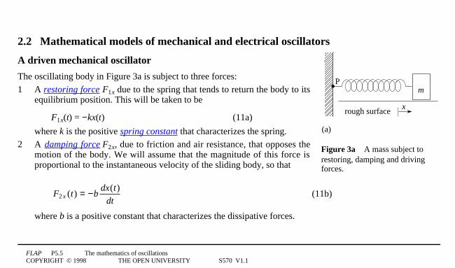
Figure 3a4A mass subject torestoring, damping and drivingforces.
A driven mechanical oscillator
The oscillating body in Figure 3a is subject to three forces:
1 A restoring force F1x due to the spring that tends to return the body to itsequilibrium position. This will be taken to be
F1x(t) = −kx(t) (11a)
where k is the positive spring constant that characterizes the spring.
2 A damping force F2x, due to friction and air resistance, that opposes themotion of the body. We will assume that the magnitude of this force isproportional to the instantaneous velocity of the sliding body, so that
F2 x (t) = −bdx(t)
dt(11b)
where b is a positive constant that characterizes the dissipative forces.
FLAP P5.5 The mathematics of oscillationsCOPYRIGHT © 1998 THE OPEN UNIVERSITY S570 V1.1
m
xrough surface
P
(a)
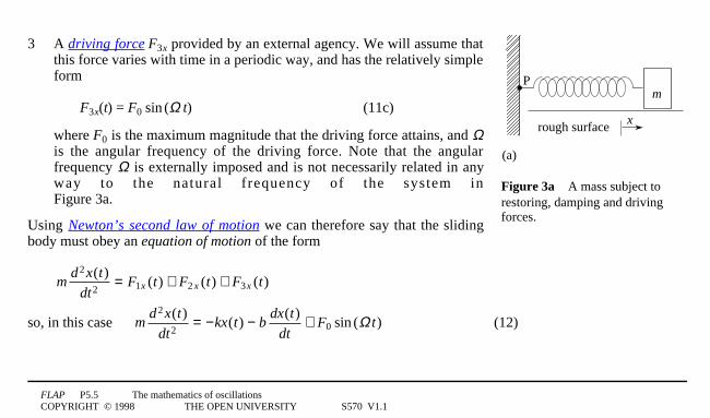
Figure 3a4A mass subject torestoring, damping and drivingforces.
3 A driving force F3x provided by an external agency. We will assume thatthis force varies with time in a periodic way, and has the relatively simpleform
F3x(t) = F01sin1(Ω1t) (11c)
where F0 is the maximum magnitude that the driving force attains, and Ωis the angular frequency of the driving force. Note that the angularfrequency Ω is externally imposed and is not necessarily related in anyway to the natural frequency of the system inFigure 3a.
Using Newton’s second law of motion we can therefore say that the slidingbody must obey an equation of motion of the form
md2 x(t)
dt2= F1x (t) + F2 x (t) + F3x (t)
so, in this case md2 x(t)
dt2= −kx(t) − b
dx(t)dt
+ F0 sin (Ω t) (12)
FLAP P5.5 The mathematics of oscillationsCOPYRIGHT © 1998 THE OPEN UNIVERSITY S570 V1.1
which can be rearranged to isolate the time-dependent driving term as follows:
md2 x(t)
dt2+ b
dx(t)dt
+ kx(t) = F0 sin (Ω t) (13)
This is known as the equation of motion of a harmonically driven linearly damped oscillator. The functionx(t) = A1sin1(Ω1t − δ01) that we introduced in Subsection 2.1 (Equation 3) to describe the steady state behaviour ofthe driven oscillator is a solution of this equation, provided we choose A and δ appropriately, as we willdemonstrate in the next subsection.

FLAP P5.5 The mathematics of oscillationsCOPYRIGHT © 1998 THE OPEN UNIVERSITY S570 V1.1
R
~
C
(b)
V(t)
L
VC(t)VR(t)
I(t)
VL(t)
Figure 3b4A simple LCR circuitcontaining a resistor, a capacitor and aninductor connected in series. At theinstant shown the current is increasingin the direction shown and thedirections (polarity) of the voltages areshown by arrows.
A series LCR circuitIn order to determine the differential equation that describes thebehaviour of the series LCR circuit of Figure 3b we need to introducetwo basic principles of circuit analysis (based on Kirchhoff’s laws):
1 In a series circuit the instantaneous current I(t) through eachcomponent is the same. The physical basis for this is the principle ofthe conservation of electric charge.
2 In a series circuit the sum of the instantaneous voltages across eachpassive component is equal to the externally supplied voltageV(t). The physical basis for this is the principle of the conservation ofenergy.

FLAP P5.5 The mathematics of oscillationsCOPYRIGHT © 1998 THE OPEN UNIVERSITY S570 V1.1
Now, we already know from Equations 4, 6 and 7 that
VR(t) = I(t)R (Eqn 4)
VC (t) = q(t)C
(Eqn 6)
VL (t) = LdI(t)
dt(Eqn 7)
So we can use the second of the two principles given above (conservation of energy.) to write
V(t) = VR(t) + VC(t) + VL(t)
Using the first principle (conservation of electric charge.), together with Equations 4, 6 and 7, this gives us
V(t) = RI(t) + q(t)C
+ LdI(t)
dt(14)
FLAP P5.5 The mathematics of oscillationsCOPYRIGHT © 1998 THE OPEN UNIVERSITY S570 V1.1
However, we also know that the current in the circuit is given by the rate of change of the charge q on the upperplate of the capacitor, so we can write
I(t) = dq(t)dt
(Eqn 8)
and hencedI(t)
dt= d2q(t)
dt2(15)
Substituting Equations 8 and 15 into Equation 14
V(t) = RI(t) + q(t)C
+ LdI(t)
dt(Eqn 14)
we see that
V(t) = Rdq(t)
dt+ 1
Cq(t) + L
d2q(t)dt2
FLAP P5.5 The mathematics of oscillationsCOPYRIGHT © 1998 THE OPEN UNIVERSITY S570 V1.1
which may be rearranged to give
Ld2q(t)
dt2+ R
dq(t)dt
+ 1C
q(t) = V(t) (16)
Finally, substituting the relevant expression for V(t) we obtain
Ld2q(t)
dt2+ R
dq(t)dt
+ 1C
q(t) = V0 sin (Ω t) (17)
Now, if you compare Equations 13 and 17
md2 x(t)
dt2+ b
dx(t)dt
+ kx(t) = F0 sin (Ω t) (Eqn 13)
you will see that they have the same form. One may be obtained from the other by making the followingsubstitutions:
q ⇔ x L ⇔ m
R ⇔ b 1/C ⇔ k V0 ⇔ F0
FLAP P5.5 The mathematics of oscillationsCOPYRIGHT © 1998 THE OPEN UNIVERSITY S570 V1.1
Note that we are not claiming some sort of mystical link between charge and displacement, or inductance andmass, but simply drawing attention to the fact that the two very different physical systems can both be describedby similar equations. It is the mathematical model that is the same in both cases, not the system it isrepresenting.
Equations 13 and 17
md2 x(t)
dt2+ b
dx(t)dt
+ kx(t) = F0 sin (Ω t) (Eqn 13)
Ld2q(t)
dt2+ R
dq(t)dt
+ 1C
q(t) = V0 sin (Ω t) (Eqn 17)
are examples (essentially the same example) of second-order differential equations with constant coefficients.(From a mathematical point of view they are also linear and inhomogeneous). Solving such equations is aninherently mathematical process, but it is of great interest to physicists since the possible solutions include thevarious forms of harmonic motion that were described in Subsection 2.1.

FLAP P5.5 The mathematics of oscillationsCOPYRIGHT © 1998 THE OPEN UNIVERSITY S570 V1.1
By differentiating Equation 16,
Ld2q(t)
dt2+ R
dq(t)dt
+ 1C
q(t) = V(t) (Eqn 16)
with respect to time, show that the instantaneous current in a series LCR circuit obeys a differential equationsimilar to that satisfied by the charge q(t).
FLAP P5.5 The mathematics of oscillationsCOPYRIGHT © 1998 THE OPEN UNIVERSITY S570 V1.1
2.3 Second-order differential equations1—1a brief reviewThis subsection describes the mathematical principles involved in solving second-order differential equationswith constant coefficients. This topic is discussed from the same point of view, but in greater detail, in the mathsstrand of FLAP.
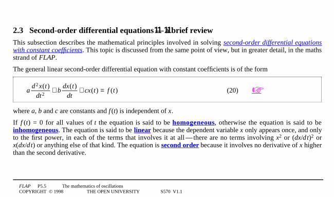
The general linear second-order differential equation with constant coefficients is of the form
ad2 x(t)
dt2+ b
dx(t)dt
+ cx(t) = f (t) (20)
where a, b and c are constants and f1(t) is independent of x.
If f1(t) = 0 for all values of t the equation is said to be homogeneous, otherwise the equation is said to beinhomogeneous. The equation is said to be linear because the dependent variable x only appears once, and onlyto the first power, in each of the terms that involves it at all1—1there are no terms involving x2 or (dx/d0t)2 orx(dx/d0t) or anything else of that kind. The equation is second order because it involves no derivative of x higherthan the second derivative.

FLAP P5.5 The mathematics of oscillationsCOPYRIGHT © 1998 THE OPEN UNIVERSITY S570 V1.1
As you can see, Equations 13 and 17
md2 x(t)
dt2+ b
dx(t)dt
+ kx(t) = F0 sin (Ω t) (Eqn 13)
Ld2q(t)
dt2+ R
dq(t)dt
+ 1C
q(t) = V0 sin (Ω t) (Eqn 17)
are both of this general form.
ad2 x(t)
dt2+ b
dx(t)dt
+ cx(t) = f (t) (Eqn 20)
In the cases that are of interest to us the constants a, b, and c are all positive, and the function f1(t) corresponds tothe external driving term.
When confronted with an equation such as Equation 20 our usual aim is to find its general solution. For such asecond-order differential equation this general solution expresses x in terms of t, the given constants that appearin the equation and two additional arbitrary constants. The values of the arbitrary constants cannot bedetermined from Equation 20 itself but must be found from supplementary conditions such as the initial values
of x and its derivative, x(0) and dx(0)
dt. These supplementary conditions are generally referred to as
boundary conditions or initial conditions as appropriate.
FLAP P5.5 The mathematics of oscillationsCOPYRIGHT © 1998 THE OPEN UNIVERSITY S570 V1.1
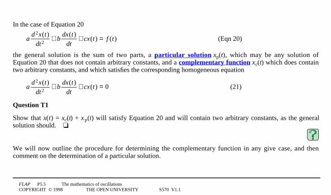
In the case of Equation 20
ad2 x(t)
dt2+ b
dx(t)dt
+ cx(t) = f (t) (Eqn 20)
the general solution is the sum of two parts, a particular solution xp(t), which may be any solution ofEquation 20 that does not contain arbitrary constants, and a complementary function xc(t) which does containtwo arbitrary constants, and which satisfies the corresponding homogeneous equation
ad2 x(t)
dt2+ b
dx(t)dt
+ cx(t) = 0 (21)
Question T1
Show that x(t) = xc(t) + xp(t) will satisfy Equation 20 and will contain two arbitrary constants, as the generalsolution should.4
We will now outline the procedure for determining the complementary function in any give case, and thencomment on the determination of a particular solution.
FLAP P5.5 The mathematics of oscillationsCOPYRIGHT © 1998 THE OPEN UNIVERSITY S570 V1.1
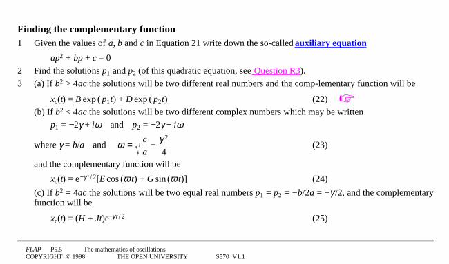
Finding the complementary function1 Given the values of a, b and c in Equation 21 write down the so-called auxiliary equation
ap2 + bp + c = 0
2 Find the solutions p1 and p2 (of this quadratic equation, see Question R3).
3 (a) If b2 > 4ac the solutions will be two different real numbers and the comp-lementary function will be
xc(t) = B1exp1(1p1t) + D1exp1(1p2t) (22) (b) If b2 < 4ac the solutions will be two different complex numbers which may be written
p1 = −2γ + iω4and4p2 = −2γ − iω
where γ = b/a4and4ω = c
a− γ 2
4(23)
and the complementary function will be
xc(t) = e−γ1t1/12[E1cos1(ω1t) + G1sin1(ω1t)] (24)
(c) If b2 = 4ac the solutions will be two equal real numbers p1 = p2 = −b/02a = −γ1/2, and the complementaryfunction will be
xc(t) = (H + Jt)e−γ1t1/12 (25)

FLAP P5.5 The mathematics of oscillationsCOPYRIGHT © 1998 THE OPEN UNIVERSITY S570 V1.1
Finding a particular solution
Determining a particular solution is generally much more difficult, and usually comes down to educatedguesswork. However, in the cases that will be of interest to us in this module the driving term f1(t) will usuallyhave the general form
f1(t) = f01sin1(Ω1t) (26)
and the particular solution will have the corresponding form
xp(t) = A1sin1(Ω1t − δ0) (27)
where A = f 0
(c a − Ω 2 )2 + (γ Ω )2 and δ = arctan
γ Ωc a − Ω 2
(28)
Note that the constants A and δ appearing in the particular solution are not arbitrary constants; their values aredetermined by the given values of a, b, c, f0 and Ω and not by any initial or boundary conditions.
Note also that for the homogeneous equation the particular solution can always be set equal to zero since f0 canthen be set equal to zero, so A = 0.
Using Equations 22 to 28 it is now possible to solve a wide a range of oscillatory problems.
FLAP P5.5 The mathematics of oscillationsCOPYRIGHT © 1998 THE OPEN UNIVERSITY S570 V1.1
Example 1 Write down the complementary function, a particular solution, and finally the general solution ofthe differential equation
Ld2q(t)
dt2+ R
dq(t)dt
+ q(t)C
= V0 sin (Ω t) (29)
when L = 1.01H, R = 5.01Ω, C = 1/61F, V0 = 0.61V and Ω = 5.01s−1.
FLAP P5.5 The mathematics of oscillationsCOPYRIGHT © 1998 THE OPEN UNIVERSITY S570 V1.1
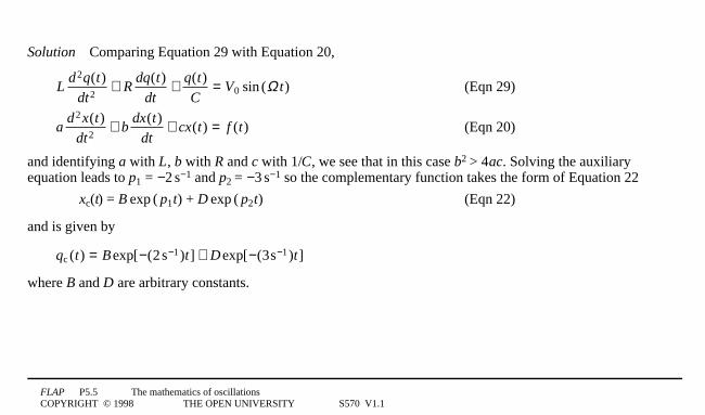
Solution4Comparing Equation 29 with Equation 20,
Ld2q(t)
dt2+ R
dq(t)dt
+ q(t)C
= V0 sin (Ω t) (Eqn 29)
ad2 x(t)
dt2+ b
dx(t)dt
+ cx(t) = f (t) (Eqn 20)
and identifying a with L, b with R and c with 1/C, we see that in this case b2 > 4ac. Solving the auxiliaryequation leads to p1 = −21s−1 and p2 = −31s−1 so the complementary function takes the form of Equation 22
xc(t) = B1exp1(1p1t) + D1exp1(1p2t) (Eqn 22)
and is given by
qc (t) = B exp[−(2 s−1)t] + Dexp[−(3s−1)t]
where B and D are arbitrary constants.
FLAP P5.5 The mathematics of oscillationsCOPYRIGHT © 1998 THE OPEN UNIVERSITY S570 V1.1
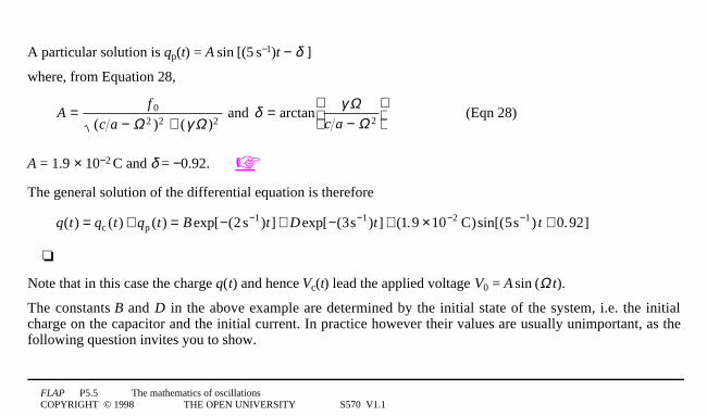
A particular solution is qp(t) = A1sin1[(51s−1)t − δ1 ]
where, from Equation 28,
A = f 0
(c a − Ω 2 )2 + (γ Ω )2 and δ = arctan
γ Ωc a − Ω 2
(Eqn 28)
A = 1.9 × 10⁻²¹C and δ = −0.92.
The general solution of the differential equation is therefore
q(t) = qc (t) + qp (t) = B exp[−(2 s−1)t] + Dexp[−(3s−1)t] + (1.9 ×10⁻² C)sin[(5s−1) t + 0.92]
4
Note that in this case the charge q(t) and hence Vc(t) lead the applied voltage V0 = A1sin1(Ω1t).
The constants B and D in the above example are determined by the initial state of the system, i.e. the initialcharge on the capacitor and the initial current. In practice however their values are usually unimportant, as thefollowing question invites you to show.

FLAP P5.5 The mathematics of oscillationsCOPYRIGHT © 1998 THE OPEN UNIVERSITY S570 V1.1
Suppose that in Example 1 we have B = 0.61C and D = 0.61C. Calculate the values of q(t), qc(t) and qp(t)when t = 01s, t = 11s, t = 31s, t = 51s and t = 81s. What do you notice about the values of q(t), qc(t) and qp(t) as tincreases? What part do B and D play in determining the eventual behaviour of q(t)?

FLAP P5.5 The mathematics of oscillationsCOPYRIGHT © 1998 THE OPEN UNIVERSITY S570 V1.1
0.08
0.10
0.060.040.02
0−0.02
54321
q/C
t/s
Figure 44The graphs of q(t) = qc(t) + qp(t) (solidcurve) and qp(t) (dashed curve) in Example 1.
Figure 4 shows the graphs of qp(t) (the dashed sinusoidalcurve) and q(t) = qc(t) + qp(t) (the solid curve). Initially theyare quite different, but for t > 4 1s they are indistinguishable.Because of this behaviour qp(t) is said to represent thesteady state behaviour, whereas qc(t) is said to represent thetransient behaviour.
The important points to notice from Example 1 are:
o the transient part of the general solution is insignificantfor large values of t, so that eventually the steady stateterm A1sin1(Ω1t − δ1) will dominate the solution;
o the constants B, D, E, G, H and J determine the initialstate of the system, but if we are only interested in whathappens for large values of t their values are irrelevant;
o the steady state term A1sin1(Ω1t − δ1) is a sinusoidal function with the same angular frequency as the drivingterm V(t).
FLAP P5.5 The mathematics of oscillationsCOPYRIGHT © 1998 THE OPEN UNIVERSITY S570 V1.1
R
~
C
(b)
V(t)
L
VC(t)VR(t)
I(t)
m
xrough surface
P
(a)
VL(t)
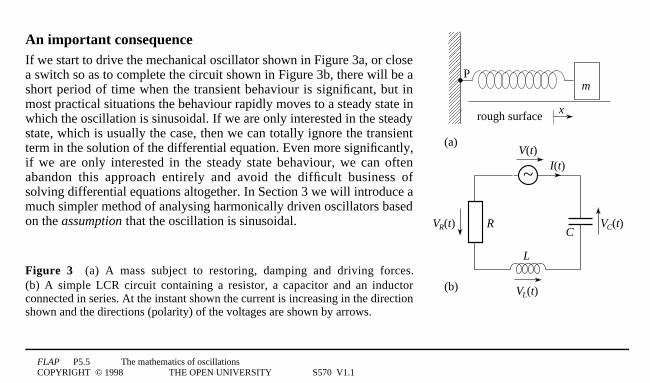
An important consequenceIf we start to drive the mechanical oscillator shown in Figure 3a, or closea switch so as to complete the circuit shown in Figure 3b, there will be ashort period of time when the transient behaviour is significant, but inmost practical situations the behaviour rapidly moves to a steady state inwhich the oscillation is sinusoidal. If we are only interested in the steadystate, which is usually the case, then we can totally ignore the transientterm in the solution of the differential equation. Even more significantly,if we are only interested in the steady state behaviour, we can oftenabandon this approach entirely and avoid the difficult business ofsolving differential equations altogether. In Section 3 we will introduce amuch simpler method of analysing harmonically driven oscillators basedon the assumption that the oscillation is sinusoidal.
Figure 34(a) A mass subject to restoring, damping and driving forces.(b) A simple LCR circuit containing a resistor, a capacitor and an inductorconnected in series. At the instant shown the current is increasing in the directionshown and the directions (polarity) of the voltages are shown by arrows.
FLAP P5.5 The mathematics of oscillationsCOPYRIGHT © 1998 THE OPEN UNIVERSITY S570 V1.1
Question T2
A mechanical oscillator satisfies the differential equation
ad2 x(t)
dt2+ b
dx(t)dt
+ cx(t) = 0
where a = 11s2, b = 41s and c = 3. Write down the auxiliary equation and solve it. Hence find the general solutionof this (homogeneous) differential equation.4
FLAP P5.5 The mathematics of oscillationsCOPYRIGHT © 1998 THE OPEN UNIVERSITY S570 V1.1
2.4 Harmonic oscillations: simple, damped and drivenIn this subsection we consider some special cases of the second-order linear differential equation
ad2 x(t)
dt2+ b
dx(t)dt
+ cx(t) = f 0 sin (Ω t) (30)
Each of the cases we consider will correspond to a particular kind of oscillatory behaviour, and may be appliedto mechanical or electrical systems (or any other system that may be similarly modelled).
b = 0, f0 = 0; the case of simple harmonic oscillation
In this case Equation 30 may be written in the form
ad2 x(t)
dt2+ cx(t) = 0 where a ≠ 0
It is conventional to rewrite this by dividing both sides by a and introducing
the natural angular frequency ω0 = c a (31)
so thatd2 x(t)
dt2+ ω0
2 x(t) = 0 (32)
FLAP P5.5 The mathematics of oscillationsCOPYRIGHT © 1998 THE OPEN UNIVERSITY S570 V1.1
In this (homogeneous) case a particular solution is xp(t) = 0. Moreover, b2 < 4ac, so the complementary function,and hence the general solution, takes the form of Equation 24 with γ = b/c = 0, and ω = c a = ω0
i.e. x(t) = E1cos1(ω00t) + G1sin1(ω00t) (33)
Show that this solution can be written in the equivalent form
x(t) = A01sin1(ω00t + φ) (34)
and hence confirm that it can be used to represent simple harmonic motion with amplitude A0, angular frequencyω0 = c a and phase constant φ.
Question T3
A simple series circuit consists of a capacitor connected in series with an inductor. If the charge on the capacitorat time t = 0 is q0, and there is no current in the circuit at that time, determine the differential equation thatdescribes the variation of q with time, write down its general solution, and show that the charge exhibits simpleharmonic oscillations with angular frequency ω0 = 1 (LC) .4
FLAP P5.5 The mathematics of oscillationsCOPYRIGHT © 1998 THE OPEN UNIVERSITY S570 V1.1
f0 = 0; the case of linearly damped oscillation
In this case Equation 30
ad2 x(t)
dt2+ b
dx(t)dt
+ cx(t) = f 0 sin (Ω t) (Eqn 30)
may be written in the form
ad2 x(t)
dt2+ b
dx(t)dt
+ cx(t) = 0 (35)
It is conventional to rewrite this by dividing both sides by a and introducing
the damping constant γ = b/a (36a)
and the natural angular frequency ω0 = c a (36b)
so thatd2 x(t)
dt2+ γ dx(t)
dt+ ω0
2 x(t) = 0 (36c)

FLAP P5.5 The mathematics of oscillationsCOPYRIGHT © 1998 THE OPEN UNIVERSITY S570 V1.1
In this case a particular solution is xp(t) = 0, and the complementary function may take any of the formsdescribed by Equations 22, 24 or 25,
xc(t) = B1exp1(1p1t) + D1exp1(1p2t) (Eqn 22)
xc(t) = e−γ1t1/12[E1cos1(ω1t) + G1sin1(ω1t)] (Eqn 24)
xc(t) = (H + Jt)e−γ1t1/12 (Eqn 25)
depending on the values of γ and ω0.
FLAP P5.5 The mathematics of oscillationsCOPYRIGHT © 1998 THE OPEN UNIVERSITY S570 V1.1
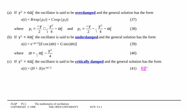
(a) If γ 2 > 4ω02 the oscillator is said to be overdamped and the general solution has the form
x(t) = B1exp1(1p1t) + C1exp 1(1p2t) (37)
where p1 = −γ2
+ γ 2
4− ω0
2 4and4 p2 = −γ2
− γ 2
4− ω0
2 (38)
(b) If γ 2 < 4ω02 the oscillator is said to be underdamped and the general solution has the form
x(t) = e−γ1t1/12[E1cos1(ω1t) + G1sin1(ω1t)] (39)
where ω = ω02 − γ 2
4(40)
(c) If γ 2 = 4ω02 the oscillator is said to be critically damped and the general solution has the form
x(t) = (H + Jt)1e−γ1t1/12 (41)
FLAP P5.5 The mathematics of oscillationsCOPYRIGHT © 1998 THE OPEN UNIVERSITY S570 V1.1
t
x(t)
t
x(t)
t
x(t)
t
x(t)
(a) (b)
(c) (d)
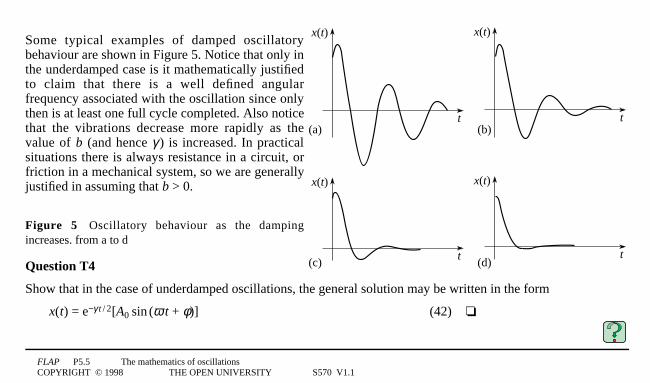
Some typical examples of damped oscillatorybehaviour are shown in Figure 5. Notice that only inthe underdamped case is it mathematically justifiedto claim that there is a well defined angularfrequency associated with the oscillation since onlythen is at least one full cycle completed. Also noticethat the vibrations decrease more rapidly as thevalue of b (and hence γ1) is increased. In practicalsituations there is always resistance in a circuit, orfriction in a mechanical system, so we are generallyjustified in assuming that b > 0.
Figure 54Oscillatory behaviour as the dampingincreases. from a to d
Question T4
Show that in the case of underdamped oscillations, the general solution may be written in the form
x(t) = e−γ1t1/12[A01sin1(ω1t + φ)] (42)4
FLAP P5.5 The mathematics of oscillationsCOPYRIGHT © 1998 THE OPEN UNIVERSITY S570 V1.1
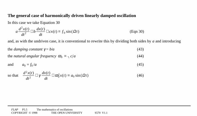
The general case of harmonically driven linearly damped oscillation
In this case we take Equation 30
ad2 x(t)
dt2 + bdx(t)
dt+ cx(t) = f 0 sin (Ω t) (Eqn 30)
and, as with the undriven case, it is conventional to rewrite this by dividing both sides by a and introducing
the damping constant γ = b/a (43)
the natural angular frequency ω0 = c a (44)
and a0 = f01/a (45)
so thatd2 x(t)
dt2+ γ dx(t)
dt+ ω0
2 x(t) = a0 sin (Ω t) (46)

FLAP P5.5 The mathematics of oscillationsCOPYRIGHT © 1998 THE OPEN UNIVERSITY S570 V1.1
In this case the general solution is the sum of a transient term (a complementary function) given by theappropriate solution to the linearly damped oscillator equation, and a steady state term (particular solution) asgiven by Equations 27 and 28
xp(t) = A1sin1(Ω1t − δ0) (Eqn 27)
A = f 0
(c a − Ω 2 )2 + (γ Ω )2 and δ = arctan
γ Ωc a − Ω 2
(Eqn 28)
with f0 replaced by a0.
Thus, in the physically important case of underdamping
x(t) = e−γ1t1/12[A01sin1(ω1t + φ)] + A1sin1(Ω1t − δ1) (47)
where A0 and φ are arbitrary constants, ω = ω02 − γ 2
4(48)
A = a0
(ω02 − Ω 2 )2 + (γ Ω )2
and δ = arctanγ Ω
ω02 − Ω 2
(49)
FLAP P5.5 The mathematics of oscillationsCOPYRIGHT © 1998 THE OPEN UNIVERSITY S570 V1.1
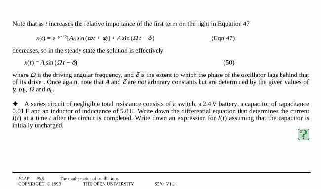
Note that as t increases the relative importance of the first term on the right in Equation 47
x(t) = e−γ1t1/12[A01sin1(ω1t + φ)] + A1sin1(Ω1t − δ1) (Eqn 47)
decreases, so in the steady state the solution is effectively
x(t) = A1sin1(Ω1t − δ) (50)
where Ω is the driving angular frequency, and δ is the extent to which the phase of the oscillator lags behind thatof its driver. Once again, note that A and δ are not arbitrary constants but are determined by the given values ofγ, ω0, Ω and a0.
A series circuit of negligible total resistance consists of a switch, a 2.41V battery, a capacitor of capacitance0.011F and an inductor of inductance of 5.01H. Write down the differential equation that determines the currentI(t) at a time t after the circuit is completed. Write down an expression for I(t) assuming that the capacitor isinitially uncharged.
FLAP P5.5 The mathematics of oscillationsCOPYRIGHT © 1998 THE OPEN UNIVERSITY S570 V1.1
R
~
(a)
V(t)I(t)
~
(b)
V(t)
L
I(t)~
(c)
V(t)
C
I(t)
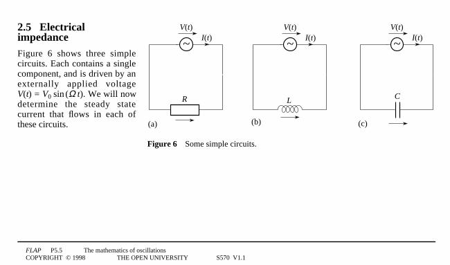
Figure 64Some simple circuits.
2.5 ElectricalimpedanceFigure 6 shows three simplecircuits. Each contains a singlecomponent, and is driven by anexternally applied voltageV(t) = V01sin1(Ω1t). We will nowdetermine the steady statecurrent that flows in each ofthese circuits.

FLAP P5.5 The mathematics of oscillationsCOPYRIGHT © 1998 THE OPEN UNIVERSITY S570 V1.1
R
~
(a)
V(t)I(t)
Figure 6a4A simplecircuit containing aresistor
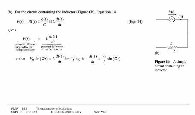
(a) For the circuit containing the resistor (Figure 6a), Equation 14
V(t) = RI(t) + q(t)C
+ LdI(t)
dt(Eqn 14)
gives
V(t) potential differencesupplied by the voltage generator
1 24 34 = RI(t) potential differenceacross the resistor
1 24 34
so that V01sin1(Ω1t) = RI(t) and therefore
I(t) = V0
Rsin (Ω t) (57)
Notice that the current I(t) and the applied voltage are in phase in this case.
FLAP P5.5 The mathematics of oscillationsCOPYRIGHT © 1998 THE OPEN UNIVERSITY S570 V1.1
~
(b)
V(t)
L
I(t)
Figure 6b4A simplecircuit containing aninductor
(b) For the circuit containing the inductor (Figure 6b), Equation 14
V(t) = RI(t) + q(t)C
+ LdI(t)
dt(Eqn 14)
gives
V(t) potential differencesupplied by the voltage generator
1 24 34 = LdI(t)
dt
potential differenceacross the inductor
1 244 344
so that V0 sin (Ω t) = LdI(t)
dt implying that
dI(t)dt
= V0
Lsin (Ω t)
FLAP P5.5 The mathematics of oscillationsCOPYRIGHT © 1998 THE OPEN UNIVERSITY S570 V1.1
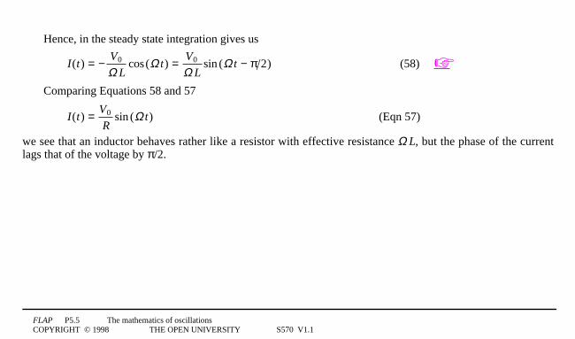
Hence, in the steady state integration gives us
I(t) = − V0
Ω Lcos(Ω t) = V0
Ω Lsin (Ω t − π 2) (58)
Comparing Equations 58 and 57
I(t) = V0
Rsin (Ω t) (Eqn 57)
we see that an inductor behaves rather like a resistor with effective resistance Ω1L, but the phase of the currentlags that of the voltage by π/2.

FLAP P5.5 The mathematics of oscillationsCOPYRIGHT © 1998 THE OPEN UNIVERSITY S570 V1.1
~
(c)
V(t)
C
I(t)
Figure 6c4A simplecircuit containing acapacitor.
(c) For the circuit containing the capacitor (Figure 6c), Equation 19
Ld2 I(t)
dt2 + RdI(t)
dt+ 1
CI(t) = dV(t)
dt(Eqn 19)
gives
I(t)C
= dV(t)dt
so that
I(t) = CdV(t)
dt= Ω CV0 cos(Ω t) = V0
1 (Ω C)sin (Ω t + π 2) (59)
Comparing Equations 59 and 57
I(t) = V0
Rsin (Ω t) (Eqn 57)
we see that a capacitor behaves rather like a resistor with effective resistance 1/(Ω 1C), but the phase of thecurrent leads that of the voltage by π/2.
FLAP P5.5 The mathematics of oscillationsCOPYRIGHT © 1998 THE OPEN UNIVERSITY S570 V1.1
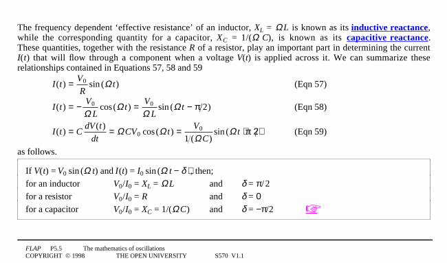
The frequency dependent ‘effective resistance’ of an inductor, XL = Ω1L is known as its inductive reactance,while the corresponding quantity for a capacitor, XC = 1/(Ω 1C), is known as its capacitive reactance.These quantities, together with the resistance R of a resistor, play an important part in determining the currentI(t) that will flow through a component when a voltage V(t) is applied across it. We can summarize theserelationships contained in Equations 57, 58 and 59
I(t) = V0
Rsin (Ω t) (Eqn 57)
I(t) = − V0
Ω Lcos(Ω t) = V0
Ω Lsin (Ω t − π 2) (Eqn 58)
I(t) = CdV(t)
dt= Ω CV0 cos(Ω t) = V0
1 (Ω C)sin (Ω t + π 2) (Eqn 59)
as follows.
If V(t) = V01sin1(Ω1t) and I(t) = I01sin1(Ω1t − δ1), then;
for an inductor V0/I0 = XL = Ω1L and δ = π0/02for a resistor V0/I0 = R and δ = 0for a capacitor V0/I0 = XC = 1/(Ω1C) and δ = −π/02
FLAP P5.5 The mathematics of oscillationsCOPYRIGHT © 1998 THE OPEN UNIVERSITY S570 V1.1
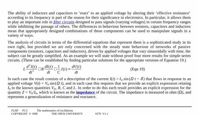
The ability of inductors and capacitors to ‘react’ to an applied voltage by altering their ‘effective resistance’according to its frequency is part of the reason for their significance in electronics. In particular, it allows themto play an important role in filter circuits designed to pass signals (varying voltages) in certain frequency rangeswhile inhibiting the passage of others. The differences in behaviour between resistors, capacitors and inductorsmean that appropriately designed combinations of these components can be used to manipulate signals in avariety of ways.
The analysis of circuits in terms of the differential equations that represent them is a sophisticated study in itsown right, but provided we are only concerned with the steady state behaviour of networks of passivecomponents (resistors, capacitors and inductors), driven by applied voltages that vary sinusoidally with time, thesubject can be greatly simplified. As an example we will state without proof four more results for simple seriescircuits. (These can be established by finding particular solutions for the appropriate versions of Equation 19.)
Ld2 I(t)
dt2 + RdI(t)
dt+ 1
CI(t) = dV(t)
dt(Eqn 19)
In each case the result consists of a description of the current I(t) = I01sin1(Ω11t − δ1) that flows in response to anapplied voltage V(t) = V01sin1(Ω11t), and in each case this requires that we provide an explicit expression relatingI0 to the known quantities V0, R, C and L. In order to do this each result provides an explicit expression for thequantity Z = V0/I0, which is known as the impedance of the circuit. The impedance is measured in ohm (Ω), andrepresents a generalization of resistance and reactance.
FLAP P5.5 The mathematics of oscillationsCOPYRIGHT © 1998 THE OPEN UNIVERSITY S570 V1.1
R
~
C
(a)
V(t)I(t)
V(t)
Figure 7a4Circuits with twocomponents: resistor andcapacitor in series.
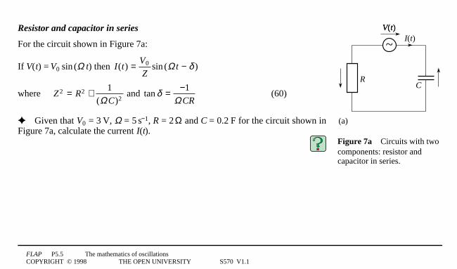
Resistor and capacitor in series
For the circuit shown in Figure 7a:
If V(t) = V01sin1(Ω1t) then I(t) = V0
Zsin (Ω t − δ )
where Z2 = R2 + 1(Ω C)2
and tan δ = −1Ω CR
(60)
Given that V0 = 31V, Ω = 51s−1, R = 21Ω and C = 0.2 1F for the circuit shown inFigure 7a, calculate the current I(t).
FLAP P5.5 The mathematics of oscillationsCOPYRIGHT © 1998 THE OPEN UNIVERSITY S570 V1.1
R
~
(b)
V(t)I(t)
V(t)
L
Figure 7b4Circuits withtwo components: resistorand inductor in series.
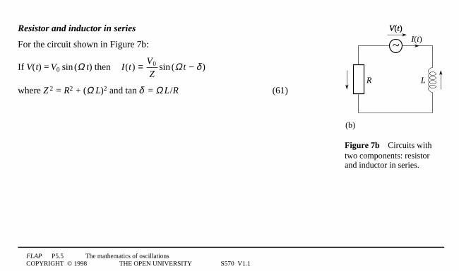
Resistor and inductor in series
For the circuit shown in Figure 7b:
If V(t) = V01sin1(Ω1t) then I(t) = V0
Zsin (Ω t − δ )
where Z12 = R2 + (Ω1L)2 and tan1δ = Ω1L0/R (61)

FLAP P5.5 The mathematics of oscillationsCOPYRIGHT © 1998 THE OPEN UNIVERSITY S570 V1.1
L
~
C
(c)
V(t)I(t)
V(t)
Figure 7c4Circuits with twocomponents: inductor andcapacitor in series.
Inductor and capacitor in series
For the circuit shown in Figure 7c:
If V(t) = V01sin1(Ω1t) then I(t) = V0
Zsin (Ω t − δ )
where
Z = 1Ω C
− Ω L and δ = π/2 if 1
Ω C< Ω L , or δ = −π/2 if
1Ω C
> Ω L (62)
FLAP P5.5 The mathematics of oscillationsCOPYRIGHT © 1998 THE OPEN UNIVERSITY S570 V1.1
R
~
C
(b)
V(t)
L
VC(t)VR(t)
I(t)
VL(t)
Figure 3b4A simple LCR circuitcontaining a resistor, a capacitor and aninductor connected in series. At theinstant shown the current is increasingin the direction shown and thedirections (polarity) of the voltages areshown by arrows.
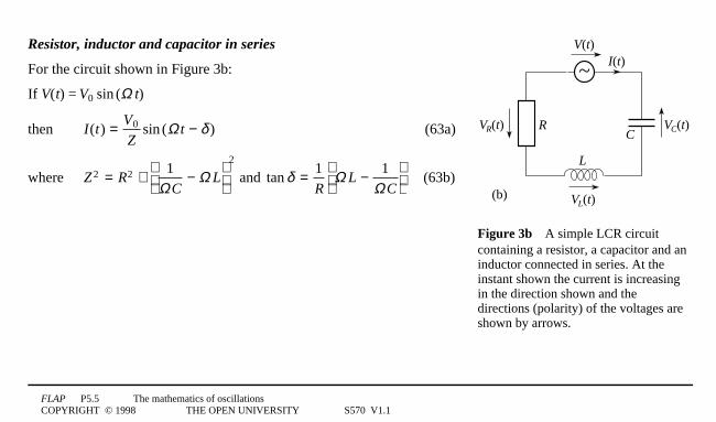
Resistor, inductor and capacitor in series
For the circuit shown in Figure 3b:
If V(t) = V01sin1(Ω1t)
then I(t) = V0
Zsin (Ω t − δ ) (63a)
where Z2 = R2 + 1Ω C
− Ω L
2
and tan δ = 1R
Ω L − 1Ω C
(63b)
FLAP P5.5 The mathematics of oscillationsCOPYRIGHT © 1998 THE OPEN UNIVERSITY S570 V1.1
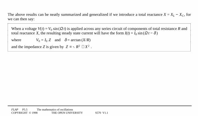
The above results can be neatly summarized and generalized if we introduce a total reactance X = XL − XC, forwe can then say:
When a voltage V(t) = V01sin1(Ω1t) is applied across any series circuit of components of total resistance R andtotal reactance X, the resulting steady state current will have the form I(t) = I01sin1(Ω1t − δ1)
where V0 = I0 Z4and4δ = arctan1(X0/R)
and the impedance Z is given by Z = R2 + X2 .

FLAP P5.5 The mathematics of oscillationsCOPYRIGHT © 1998 THE OPEN UNIVERSITY S570 V1.1
Ω L
1/Ω CR
R
(a) (b) R
δ
Z
δ
Z
(c) (d)R
(e)
δ
Z1/Ω C Ω L
Ω L
1/Ω C
Ω L= 1/Ω C
Figure 84Geometrical interpretations of Z and δ in terms of XL, XC and R.
It is possible to give a simple geometric interpretation to the relationship between impedance, resistance andreactance. This is indicated in Figure 8a, where XL is treated as a ‘vector quantity’ directed vertically upwards,XC is treated as a vector directed vertically downwards, and R is treated as a vector directed to the right.(The length of each ‘vector’ represents the relevant value of resistance or reactance.)
As Figures 8b to 8e indicate, the value of Z in each of the cases discussed above will be represented by thelength of the ‘vector sum’ of XL, XC and R, and the value of δ will be given by the angle (measured in theanticlockwise direction) from the horizontal axis to the ‘vector’ representing Z . We will return to thisgeometric interpretation of impedance in Section 3.
FLAP P5.5 The mathematics of oscillationsCOPYRIGHT © 1998 THE OPEN UNIVERSITY S570 V1.1
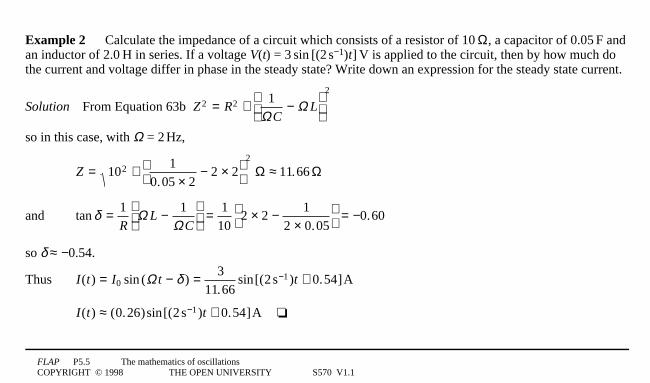
Example 2 Calculate the impedance of a circuit which consists of a resistor of 101Ω, a capacitor of 0.051F andan inductor of 2.01H in series. If a voltage V(t) = 31sin1[(21s−1)0t]1V is applied to the circuit, then by how much dothe current and voltage differ in phase in the steady state? Write down an expression for the steady state current.
Solution4From Equation 63b Z2 = R2 + 1Ω C
− Ω L
2
so in this case, with Ω = 21Hz,
Z = 102 + 10.05 × 2
− 2 × 2
2
Ω ≈ 11.66 Ω
and tan δ = 1R
Ω L − 1Ω C
= 110
2 × 2 − 12 × 0.05
= −0.60
so δ ≈ −0.54.
Thus I(t) = I0 sin (Ω t − δ ) = 311.66
sin[(2 s−1)t + 0.54]A
I(t) ≈ (0.26)sin[(2 s−1)t + 0.54]A4
FLAP P5.5 The mathematics of oscillationsCOPYRIGHT © 1998 THE OPEN UNIVERSITY S570 V1.1
R
~
C
(b)
V(t)
L
VC(t)VR(t)
I(t)
VL(t)
Figure 3b4A simple LCR circuitcontaining a resistor, a capacitor and aninductor connected in series. At theinstant shown the current is increasingin the direction shown and thedirections (polarity) of the voltages areshown by arrows.
Question T5
When the series LCR circuit of Figure 3b is driven by an applied voltageV(t) = V01sin1(Ω1t), the current I(t) satisfies Equation 19.
Ld2 I(t)
dt2 + RdI(t)
dt+ 1
CI(t) = dV(t)
dt(Eqn 19)
Show that Equation 63
I(t) = V0
Zsin (Ω t − δ ) (Eqn 63a)
Z2 = R2 + 1Ω C
− Ω L
2
and tan δ = 1R
Ω L − 1Ω C
(Eqn 63b)
really does provide a particular solution of this equation, as claimedabove. 4

FLAP P5.5 The mathematics of oscillationsCOPYRIGHT © 1998 THE OPEN UNIVERSITY S570 V1.1
Question T6
Calculate the impedance of a circuit which consists of a resistor of 5.01Ω, a capacitor of 1/6 F and an inductor of
1.01H in series.
A voltage V(t) = 35 sin[(5s − 1) t]V is applied to the circuit and the current is allowed to reach its steady state.
By how much do the steady state current and voltage differ in phase? Write down an expression for the steadystate current. Compare your answer with that of Example 1.4
FLAP P5.5 The mathematics of oscillationsCOPYRIGHT © 1998 THE OPEN UNIVERSITY S570 V1.1
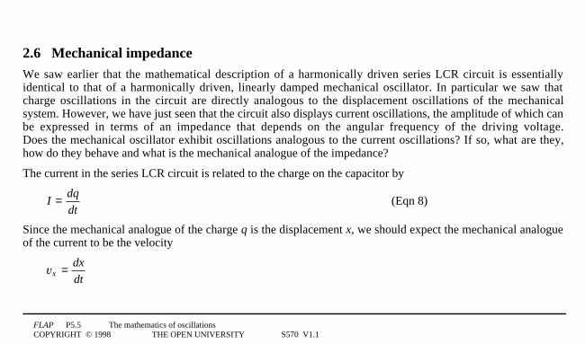
2.6 Mechanical impedanceWe saw earlier that the mathematical description of a harmonically driven series LCR circuit is essentiallyidentical to that of a harmonically driven, linearly damped mechanical oscillator. In particular we saw thatcharge oscillations in the circuit are directly analogous to the displacement oscillations of the mechanicalsystem. However, we have just seen that the circuit also displays current oscillations, the amplitude of which canbe expressed in terms of an impedance that depends on the angular frequency of the driving voltage.Does the mechanical oscillator exhibit oscillations analogous to the current oscillations? If so, what are they,how do they behave and what is the mechanical analogue of the impedance?
The current in the series LCR circuit is related to the charge on the capacitor by
I = dq
dt(Eqn 8)
Since the mechanical analogue of the charge q is the displacement x, we should expect the mechanical analogueof the current to be the velocity
vx = dx
dt

FLAP P5.5 The mathematics of oscillationsCOPYRIGHT © 1998 THE OPEN UNIVERSITY S570 V1.1
m
xrough surface
P
(a)
Figure 3a4A mass subject torestoring, damping and drivingforces.
According to Equation 19
Ld2 I(t)
dt2 + RdI(t)
dt+ 1
CI(t) = dV(t)
dt(Eqn 19)
sinusoidally driven current oscillations satisfy a differential equation of theform
Ld2 I(t)
dt2+ R
dI(t)dt
+ I(t)C
= ΩV0 cos(Ω t)
Write down the analogous differential equation that you might expectmechanical velocity oscillations to satisfy, and show that the mechanicaloscillator of Figure 3a does in fact obey such an equation.

FLAP P5.5 The mathematics of oscillationsCOPYRIGHT © 1998 THE OPEN UNIVERSITY S570 V1.1
Using the description of the current oscillations given in the last subsection, write down the correspondingdescription of the velocity oscillations in the driven mechanical oscillator, and hence identify the mechanicalimpedance Zm.
By analogy with the electrical case, it is possible to identify the mass m and the spring constant k as ‘reactive’parts of the mechanical oscillator, since their contribution to the mechanical impedance depends on the angularfrequency of the driving force.

FLAP P5.5 The mathematics of oscillationsCOPYRIGHT © 1998 THE OPEN UNIVERSITY S570 V1.1
2.7 Resonance and driven oscillationsThe displacement oscillations described by Equations 49 and 50,
A = a0
(ω02 − Ω 2 )2 + (γ Ω )2
and δ = arctanγ Ω
ω02 − Ω 2
(Eqn 49)
x(t) = A1sin1(Ω1t − δ) (Eqn 50)
and the velocity oscillations described by Equations 65 and 66,
vx = v01sin1(Ω1t − δ1) (Eqn 65)
tan δ = 1b
Ωm − k
Ω
(Eqn 66)
both have an amplitude that depends sensitively on the angular frequency Ω of the driving force. The charge andcurrent oscillations in the driven LCR circuit show a similar sensitivity to the angular frequency of the drivingvoltage.

FLAP P5.5 The mathematics of oscillationsCOPYRIGHT © 1998 THE OPEN UNIVERSITY S570 V1.1
decreasingvalues of R
Ω1LC
I0
As an example of this behaviour, Figure 9 shows the way in which the amplitudeI0 of the steady state current varies with driving frequency for fixed values of C, Land V0 at a variety of values of R. It is clear from Equation 63
I(t) = V0
Zsin (Ω t − δ ) (Eqn 63a)
Z2 = R2 + 1Ω C
− Ω L
2
and tan δ = 1R
Ω L − 1Ω C
(Eqn 63b)
that in this case, for any fixed value of R , the impedance is a minimum and thecurrent amplitude a maximum when Ω = 1 (LC) .
This is an example of the phenomenon of resonance, the production of a largeresponse in a driven oscillator by driving it at a frequency close to the naturalfrequency it would have in the absence of any driving or damping. As you can see,the smaller the value of R, the taller and narrower the peak, i.e. the sharper theresonance. In this particular case the resonant frequency at which the response isa maximum is identical to the natural frequency ω0 = 1 (LC) , but that is notalways the case.
Figure 94The amplitude of the current I0 as a function of the driving angular frequency Ω.
FLAP P5.5 The mathematics of oscillationsCOPYRIGHT © 1998 THE OPEN UNIVERSITY S570 V1.1
The current and velocity oscillations have a resonant frequency that is independent of the resistance ordamping (R and b respectively). Is the same true of the resonant frequency of the charge and displacementoscillations?If not, what is the relationship between the resonant frequency, the natural frequency and the resistance ordamping in this case?
Question T7
A radio aerial for BBC Radio 4 contains an inductor L = 0.0011H (i.e. 1.01mH) and a variable capacitor C inseries. The transmitter induces a voltage in the aerial, and produces a potential difference V(t) = V01sin1(ω1t)across the open circuit, where ω = 2π × 1981kHz. To what value should the capacitor be set in order to maximizethe amplitude of the current?4
FLAP P5.5 The mathematics of oscillationsCOPYRIGHT © 1998 THE OPEN UNIVERSITY S570 V1.1
3 Oscillations and complex numbersComplex numbers are often used in the analysis of sinusoidal oscillations. They can greatly simplify manyproblems, so much so that they constitute the standard approach in most advanced work. As you pursue yourstudies of physics it is inevitable that you will frequently encounter discussions of oscillatory phenomena basedon complex methods. This is particularly true in quantum physics, where complex numbers are not just useful,but essentially unavoidable.
3.1 Complex numbers1—1a brief review1 Any complex number, z, may be written as
z = x + iy where x and y are real numbers and i satisfies i2 = −1.
2 If z = x + iy (with x and y real) then x is known as the real part of z, written as Re(z), and y is known as theimaginary part of z, written as Im(z). Thus,
z = Re(z) + iIm(z)
3 Complex numbers obey the rules of normal algebra except that i2 can be replaced by −1 whenever itappears.
FLAP P5.5 The mathematics of oscillationsCOPYRIGHT © 1998 THE OPEN UNIVERSITY S570 V1.1
4 The complex conjugate of z (written z*) is defined by
z* = x − iy = Re(z) − iIm(z)
5 The modulus of z = x + iy (written as |1z1|) is defined by
| z | = x2 + y2 = [Re(z)]2 + [Im(z)]2
6 For arbitrary complex numbers z and w
Re(z) = 12
(z + z*) Im(z) = 12i
(z − z*)
(zw)* = z*w* (z*)* = z4and4|1z1|2 = zz*
7 A complex number, z = x + iy, is said to be in Cartesian form or a Cartesian representation.
Such a complex number may also be written in the form,
z = r1(cos1θ + i1sin1θ)
where r and θ are real numbers, in which case it is said to be in polar form or a polar representation. Whenwritten in polar form, the modulus of z is then given by |1z1| = r, and θ is referred to as the argument of z(written as arg(z)). Adding 2π to the argument of a complex number does not change that complex number.The principal value of the argument of a complex number is the value θ which lies in the range −π < θ ≤ π.
FLAP P5.5 The mathematics of oscillationsCOPYRIGHT © 1998 THE OPEN UNIVERSITY S570 V1.1
8 We can convert from Cartesian to polar form using
r = x2 + y2 , cosθ = x
x2 + y2 and sin θ = y
x2 + y2
and from polar to Cartesian form by means of
x = r1cos1θ4and4y = r1sin1θ9 A complex number can be represented by a point on an Argand diagram (complex plane) by using (x, y) as
the Cartesian coordinates or (r, θ) as the polar coordinates of the point. (By convention, θ is measuredanticlockwise from the positive x-axis.)
10 A complex number may also be written in exponential form or exponential representation by usingEuler’s formula
e0i1θ = cos1θ + i1sin1θ
If z = r1ei1θ, then |1z1| = r, arg(z) = θ and z* = r1e−i1θ.
FLAP P5.5 The mathematics of oscillationsCOPYRIGHT © 1998 THE OPEN UNIVERSITY S570 V1.1
11 Addition and subtraction of complex numbers is simplest in Cartesian form:
z + w = (x + iy) + (u + iv) = (x + u) + i0( 0y + v)
z − w = (x + iy) − (u + iv) = (x − u) + i0(0y − v)
Multiplication and division of complex numbers is simplest in exponential form:
zw = (r1e0i1θ)0(s1e0iφ) = (rs)10e0i1(θ + φ0)
z/w = (r1e0i1θ)/(s1e0i1φ) = (r/s)1ei01(θ − φ0)
The following result, known as Demoivre’s theorem is valid for any real value of n
e0n 1i1θ = (cos1θ + i1sin1θ0)n = cos1(nθ0) + i1sin1(nθ0)

FLAP P5.5 The mathematics of oscillationsCOPYRIGHT © 1998 THE OPEN UNIVERSITY S570 V1.1
3.2 Complex impedance
Study comment It is important to appreciate that in the following discussion of electrical circuits we are only interested inthe steady state, and we are therefore assuming that sufficient time has elapsed for the transient part of the current to benegligible.In this subsection when we refer to ‘the current’ we always mean the steady state current. Since we are only concerned withthe steady state, the phase of the applied voltage is unimportant1—1it is the phase difference between the applied voltage andthe current that is critical. Previously it was convenient to assume that the applied voltage was of the form V0 1sin1(Ω1t),but here it is more conventional to choose V01cos1(ω1t), and to describe the steady state current by I0 1cos1(ω1t − δ 1).The effect is minimal and serves only to make the mathematics a little easier, and more standard.
The impedance Z and phase lag δ determine the relationship between the voltage that drives the LCR circuit ofFigure 3b, and the steady state current it eventually produces. There is however a very simple method ofdetermining these quantities in terms of the values of R, C and L, and, as we will see, this new method may beused to analyse far more complicated circuits.

FLAP P5.5 The mathematics of oscillationsCOPYRIGHT © 1998 THE OPEN UNIVERSITY S570 V1.1
Ω L
1/Ω CR
R
(a) (b) R
δ
Z
δ
Z
(c) (d)R
(e)
δ
Z1/Ω C Ω L
Ω L
1/Ω C
Ω L= 1/Ω C
Figure 84Geometrical interpretations of Z and δ in terms of XL, XC and R.
We begin by referring once again to Figure 8, the geometric interpretation of impedance. If we interpret thedirection assigned to the ‘vector’ representing the resistance R as the real axis of an Argand diagram, and if weallow the heads of the various ‘vectors’ in Figure 8 to denote complex numbers, then the values of both Z and δcan be found very easily as the modulus and argument of the sum of the various complex numbers involved.
Adopting this approach, and noting that in this case we are dealing with an applied voltage with angularfrequency ω, we can identify the following complex quantities from Figure 8a
o the complex inductive reactance iω1Lo the complex capacitive reactance −0i0/ω1Co the resistance (a real quantity) R

FLAP P5.5 The mathematics of oscillationsCOPYRIGHT © 1998 THE OPEN UNIVERSITY S570 V1.1
Ω L
1/Ω CR
R
(a) (b) R
δ
Z
δ
Z
(c) (d)R
(e)
δ
Z1/Ω C Ω L
Ω L
1/Ω C
Ω L= 1/Ω C
Figure 84Geometrical interpretations of Z and δ in terms of XL, XC and R.
We can then define a new quantity, the complex impedance Z of a series LCR circuit by the relation
Z = R + iω L + −i
ω C
= R + i ω L − 1ω C
(67)
From Figures 8b to 8e it can be seen that this complex impedance has the following properties:
o its modulus is equal to the impedance, so |1Z1| = Z o its argument is equal to the phase lag, so arg(Z1) = δ
FLAP P5.5 The mathematics of oscillationsCOPYRIGHT © 1998 THE OPEN UNIVERSITY S570 V1.1
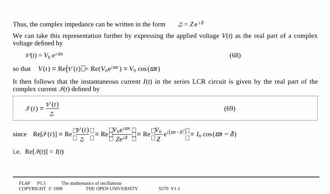
Thus, the complex impedance can be written in the form Z = Z1e 1i1δ
We can take this representation further by expressing the applied voltage V(t) as the real part of a complexvoltage defined by
V1(t) = V01e0i1ω1t (68)
so that V(t) = Re V (t)( ) = Re(V0eiω t ) = V0 cos(ω t)
It then follows that the instantaneous current I(t) in the series LCR circuit is given by the real part of thecomplex current ((t) defined by
( (t) = V (t)
Z(69)
since Re[( (t)] = Re
V (t)Z
= Re
V0eiω t
Zeiδ
= ReV0
Zei ω t −δ( )
= I0 cos(ω t − δ )
i.e. Re[((t)] = I(t)
FLAP P5.5 The mathematics of oscillationsCOPYRIGHT © 1998 THE OPEN UNIVERSITY S570 V1.1
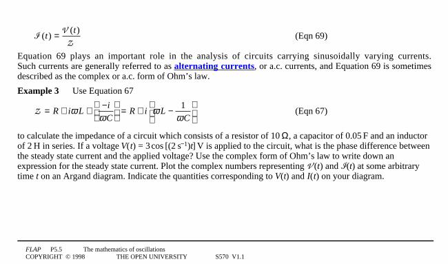
( (t) = V (t)
Z(Eqn 69)
Equation 69 plays an important role in the analysis of circuits carrying sinusoidally varying currents.Such currents are generally referred to as alternating currents, or a.c. currents, and Equation 69 is sometimesdescribed as the complex or a.c. form of Ohm’s law.
Example 3 Use Equation 67
Z = R + iω L + −i
ω C
= R + i ω L − 1ω C
(Eqn 67)
to calculate the impedance of a circuit which consists of a resistor of 101Ω, a capacitor of 0.051F and an inductorof 21H in series. If a voltage V(t) = 31cos1[(21s−1)t]1V is applied to the circuit, what is the phase difference betweenthe steady state current and the applied voltage? Use the complex form of Ohm’s law to write down anexpression for the steady state current. Plot the complex numbers representing V1(t) and ((t) at some arbitrarytime t on an Argand diagram. Indicate the quantities corresponding to V(t) and I(t) on your diagram.
FLAP P5.5 The mathematics of oscillationsCOPYRIGHT © 1998 THE OPEN UNIVERSITY S570 V1.1
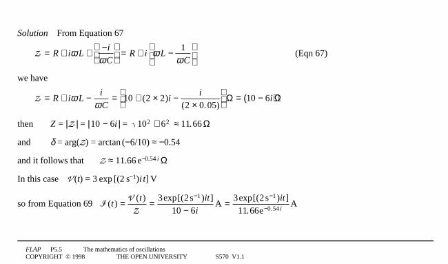
Solution4From Equation 67
Z = R + iω L + −i
ω C
= R + i ω L − 1ω C
(Eqn 67)
we have
Z = R + iω L − i
ω C= 10 + (2 × 2)i − i
(2 × 0.05)
Ω = (10 − 6i)Ω
then Z = |1Z1| = |110 − 6i1| = 102 + 62 ≈ 11.66 Ω
and δ = arg(Z) = arctan1(−6/10) ≈ −0.54
and it follows that Z ≈ 11.661e−0.541i1Ω
In this case V1(t) = 31exp1[(21s−1)0i0t]1V
so from Equation 69 ( (t) = V (t)
Z= 3exp[(2 s−1)it]
10 − 6iA = 3exp[(2 s−1)it]
11.66e−0.54 iA
FLAP P5.5 The mathematics of oscillationsCOPYRIGHT © 1998 THE OPEN UNIVERSITY S570 V1.1
φ
ωt
((t)
V (t)
((t)V (t)
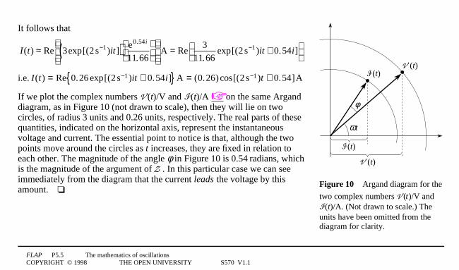
Figure 104Argand diagram for the
two complex numbers V1(t)/V and((t)/A. (Not drawn to scale.) Theunits have been omitted from thediagram for clarity.
It follows that
I(t) ≈ Re 3exp[(2 s−1)it]( ) e0.54i
11.66
A = Re
311.66
exp[(2 s−1)it + 0.54i]
i.e. I(t) = Re 0.26 exp[(2 s−1)it + 0.54i] A = (0.26)cos[(2 s−1)t + 0.54]A
If we plot the complex numbers V1(t)/V and ((t)/A on the same Arganddiagram, as in Figure 10 (not drawn to scale), then they will lie on twocircles, of radius 3 units and 0.26 units, respectively. The real parts of thesequantities, indicated on the horizontal axis, represent the instantaneousvoltage and current. The essential point to notice is that, although the twopoints move around the circles as t increases, they are fixed in relation toeach other. The magnitude of the angle φ in Figure 10 is 0.541radians, whichis the magnitude of the argument of Z . In this particular case we can seeimmediately from the diagram that the current leads the voltage by thisamount.4

FLAP P5.5 The mathematics of oscillationsCOPYRIGHT © 1998 THE OPEN UNIVERSITY S570 V1.1
Aside It is worth noting that the conversion of complex numbers from Cartesian to exponential (or polar) form that was atthe heart of this example is available as a standard function on many modern calculators. My calculator stores a complexnumber 3 + 5i as (3 5) so to check this example I keyed in:
(10, 0) for the 101Ω resistance and then stored it as R,
(0, 2 × 2) for the iω1L term and stored it as Z1,
then 0, − 12 × 0.05
for the 1/(iω1C) term and stored it as Z2.
Then I calculated 3/(R + Z1 + Z2) and finally converted it into polar form using a function labelled c → p on my calculator.You may find that you can perform similar calculations on your own calculator.
If you compare the solution to Example 3 with the solution to Example 2, you will find that the answers are thesame (apart from a change of sin to cos), but this method is simpler.

FLAP P5.5 The mathematics of oscillationsCOPYRIGHT © 1998 THE OPEN UNIVERSITY S570 V1.1
Question T8
Use Equation 67
Z = R + iω L + −i
ω C
= R + i ω L − 1ω C
(Eqn 67)
to calculate the impedance of a resistor R = 151Ω, a capacitor of C = 51µF and an inductor L = 41mH in series.Find the complex impedance, Z, and hence find 1/Z, when a voltage V(t) = 101cos1[(1041s−1)t]1V is applied to thecircuit. By how much do the steady state current and the applied voltage differ in phase?
Write down an expression for the steady state current.4
FLAP P5.5 The mathematics of oscillationsCOPYRIGHT © 1998 THE OPEN UNIVERSITY S570 V1.1
R
~
C
V(t)
L
IR(t)I(t)
IL(t)
IC(t)
Figure 114Three components inparallel.
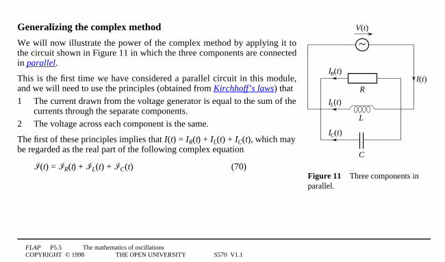
Generalizing the complex method
We will now illustrate the power of the complex method by applying it tothe circuit shown in Figure 11 in which the three components are connectedin parallel.
This is the first time we have considered a parallel circuit in this module,and we will need to use the principles (obtained from Kirchhoff’s laws) that
1 The current drawn from the voltage generator is equal to the sum of thecurrents through the separate components.
2 The voltage across each component is the same.
The first of these principles implies that I(t) = IR(t) + IL(t) + IC(t), which maybe regarded as the real part of the following complex equation
((t) = (R(t) + (L(t) + (C(t) (70)
FLAP P5.5 The mathematics of oscillationsCOPYRIGHT © 1998 THE OPEN UNIVERSITY S570 V1.1
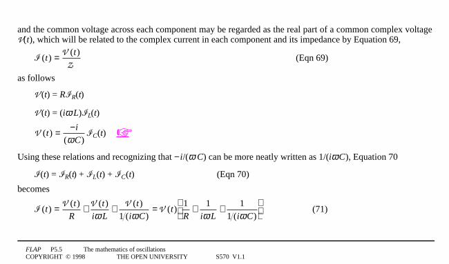
and the common voltage across each component may be regarded as the real part of a common complex voltageV(t), which will be related to the complex current in each component and its impedance by Equation 69,
( (t) = V (t)
Z(Eqn 69)
as follows
V1(t) = R(R(t)
V1(t) = (iω1L)(L(t)
V (t) = −i
(ω C)(C(t)
Using these relations and recognizing that −0i/(ω C) can be more neatly written as 1/(iω1C), Equation 70
((t) = (R(t) + (L(t) + (C(t) (Eqn 70)
becomes
( (t) = V (t)
R+ V (t)
iω L+ V (t)
1 (iω C)= V (t)
1R
+ 1iω L
+ 11 (iω C)
(71)
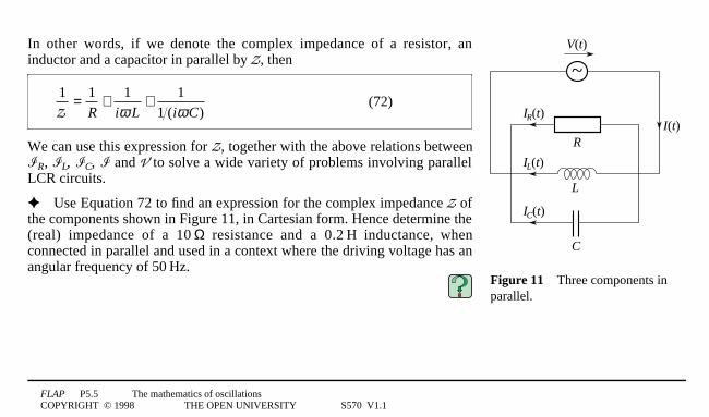
FLAP P5.5 The mathematics of oscillationsCOPYRIGHT © 1998 THE OPEN UNIVERSITY S570 V1.1
R
~
C
V(t)
L
IR(t)I(t)
IL(t)
IC(t)
Figure 114Three components inparallel.
In other words, if we denote the complex impedance of a resistor, aninductor and a capacitor in parallel by Z, then
1Z
= 1R
+ 1iω L
+ 11 (iω C)
(72)
We can use this expression for Z, together with the above relations between(R, (L, (C, ( and V to solve a wide variety of problems involving parallelLCR circuits.
Use Equation 72 to find an expression for the complex impedance Z ofthe components shown in Figure 11, in Cartesian form. Hence determine the(real) impedance of a 101Ω resistance and a 0.21H inductance, whenconnected in parallel and used in a context where the driving voltage has anangular frequency of 501Hz.
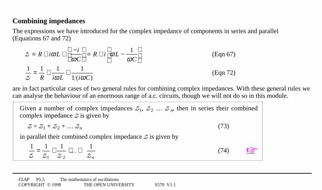
FLAP P5.5 The mathematics of oscillationsCOPYRIGHT © 1998 THE OPEN UNIVERSITY S570 V1.1
Combining impedancesThe expressions we have introduced for the complex impedance of components in series and parallel (Equations 67 and 72)
Z = R + iω L + −i
ω C
= R + i ω L − 1ω C
(Eqn 67)
1Z
= 1R
+ 1iω L
+ 11 (iω C)
(Eqn 72)
are in fact particular cases of two general rules for combining complex impedances. With these general rules wecan analyse the behaviour of an enormous range of a.c. circuits, though we will not do so in this module.
Given a number of complex impedances Z1, Z02 … Z 0n, then in series their combinedcomplex impedance Z is given by
Z = Z1 + Z02 + … Z0n (73)
in parallel their combined complex impedance Z is given by
1Z
= 1Z1
+ 1Z 2
+ … + 1Zn
(74)
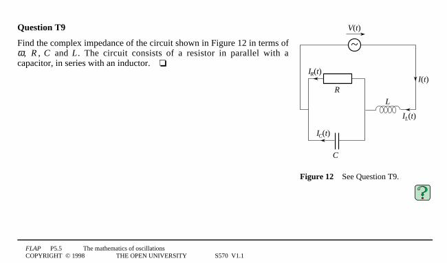
FLAP P5.5 The mathematics of oscillationsCOPYRIGHT © 1998 THE OPEN UNIVERSITY S570 V1.1
R
~
C
V(t)
L
IR(t)I(t)
IC(t)
IL(t)
Figure 124See Question T9.
Question T9
Find the complex impedance of the circuit shown in Figure 12 in terms ofω, R , C and L. The circuit consists of a resistor in parallel with acapacitor, in series with an inductor.4
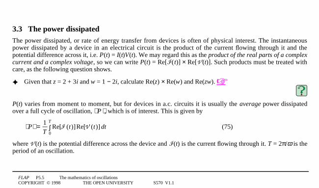
FLAP P5.5 The mathematics of oscillationsCOPYRIGHT © 1998 THE OPEN UNIVERSITY S570 V1.1
3.3 The power dissipatedThe power dissipated, or rate of energy transfer from devices is often of physical interest. The instantaneouspower dissipated by a device in an electrical circuit is the product of the current flowing through it and thepotential difference across it, i.e. P(t) = I(t)V(t). We may regard this as the product of the real parts of a complexcurrent and a complex voltage, so we can write P(t) = Re[(0(t)] × Re[V1(t)]. Such products must be treated withcare, as the following question shows.
Given that z = 2 + 3i and w = 1 − 2i, calculate Re(z) × Re(w) and Re(zw).
P(t) varies from moment to moment, but for devices in a.c. circuits it is usually the average power dissipatedover a full cycle of oscillation, ⟨ 1P1⟩, which is of interest. This is given by
⟨P⟩ = 1
TRe[( (t)]Re[V (t)]
0
T
∫ dt (75)
where V1(t) is the potential difference across the device and ((t) is the current flowing through it. T = 2π/ω is theperiod of an oscillation.

FLAP P5.5 The mathematics of oscillationsCOPYRIGHT © 1998 THE OPEN UNIVERSITY S570 V1.1
We can simplify this result by introducing two new constants which may be complex, V0 and ( 0.Any sinusoidally varying voltage may then be written as the real part of
V0(t) = V01e0i1ω1t (76)
and any sinusoidally varying current as the real part of
((t) = (01e0i1ω1t (77)
With the aid of these generalized complex expressions, it is possible to show that Equation 75
⟨P⟩ = 1
TRe[( (t)]Re[V (t)]
0
T
∫ dt (Eqn 75)
leads to the following useful result :
⟨P⟩ = 1
2Re(( 0
*V 0 ) (78)
If you are interested in knowing how this formula is obtained you can answer the following (fairly difficult)question. If not, you can simply use Equation 78 to answer Question T11.

FLAP P5.5 The mathematics of oscillationsCOPYRIGHT © 1998 THE OPEN UNIVERSITY S570 V1.1
Question T10
Prove this claim.
i.e. that ⟨P⟩ = 1
2Re(( 0
*V 0 ) (Eqn 78)
(Hint: First show that eniω t
0
T
∫ dt = 0 for any non-zero integer, n, and then use that result to derive Equation 78
from Equation 75.)
⟨P⟩ = 1
TRe[( (t)]Re[V (t)]
0
T
∫ dt (Eqn 75) 4
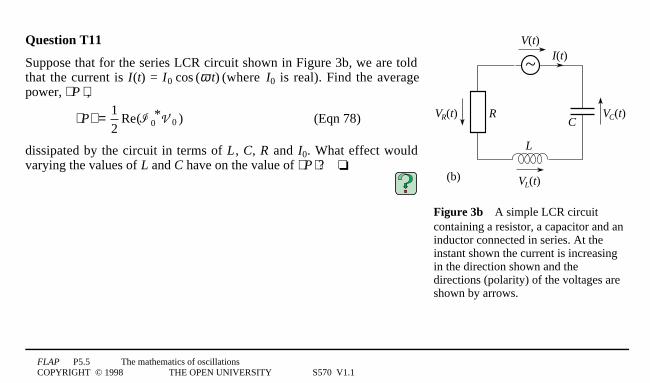
FLAP P5.5 The mathematics of oscillationsCOPYRIGHT © 1998 THE OPEN UNIVERSITY S570 V1.1
R
~
C
(b)
V(t)
L
VC(t)VR(t)
I(t)
VL(t)
Figure 3b4A simple LCR circuitcontaining a resistor, a capacitor and aninductor connected in series. At theinstant shown the current is increasingin the direction shown and thedirections (polarity) of the voltages areshown by arrows.
Question T11
Suppose that for the series LCR circuit shown in Figure 3b, we are toldthat the current is I(t) = I01cos1(ω1t) (where I0 is real). Find the averagepower, ⟨ 1P1⟩ ,
⟨P⟩ = 1
2Re(( 0
*V 0 ) (Eqn 78)
dissipated by the circuit in terms of L, C, R and I0. What effect wouldvarying the values of L and C have on the value of ⟨ 1P1⟩?4
FLAP P5.5 The mathematics of oscillationsCOPYRIGHT © 1998 THE OPEN UNIVERSITY S570 V1.1
4 Superposed oscillations and complex algebraSimple harmonic oscillation is common in nature, and situations often arise in which an oscillating system issubject to several independent influences each of which tends to promote SHM. For example, the steady statecurrent in a circuit might be the response of two independent sinusoidal voltage supplies, each of which drivesthe circuit with a characteristic amplitude, angular frequency and phase constant. In such cases, provided thecircuit concerned has the property of linearity, i.e. provided its behaviour can be modelled by linear differentialequations, the response of the circuit at any time will be the sum of the responses it would have shown to each ofthe applied voltages independently. This general feature of the behaviour of linear systems is enshrined in thesuperposition principle:
When several oscillations are added, the resulting disturbance at any time is the sum of the disturbances dueto each oscillation at that time.
In view of the wide applicability of the superposition principle it is hardly surprising that the problem of addingor rather superposing simple harmonic oscillations is frequently encountered in physics. From a mathematicalpoint of view these additions can be carried out in a number of ways (the use of phasors and of trigonometricidentities are both explored elsewhere in FLAP); however when large numbers of oscillations must be addedtogether it is often advantageous to make use of complex methods. It is this process that we will discuss in thissection.

FLAP P5.5 The mathematics of oscillationsCOPYRIGHT © 1998 THE OPEN UNIVERSITY S570 V1.1
In what follows we will make use of the following general result from the arithmetic of complex numbers.
If α1 and α2 are arbitrary real numbers, then
exp1(iα 1) + exp1(iα 02)
= exp1[i(α1 + α2)/2]1exp 1[i(α1 − α2)/2] + exp1[i(α1 + α2)/2]1exp 1[−i(α1 − α2)/2]
= exp1[i(α1 + α2)/2]1exp1[i(α1 − α2)/2] + exp1[−i(α1 − α2)/2]
= exp1[i(α1 + α2)/2]1cos1[(α1 − α2)/2] + i1sin1[(α1 − α2)/2]
+ cos1[(α1 − α2)/2] − i1sin1[(α1 − α2)/2]
i.e. exp1(iα 1) + exp1(iα2) = 21exp1[i(α1 + α2)/2]1cos1[(α1 − α2)/2] (79)
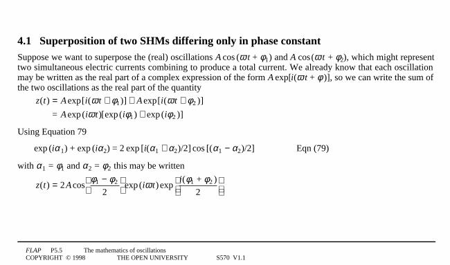
FLAP P5.5 The mathematics of oscillationsCOPYRIGHT © 1998 THE OPEN UNIVERSITY S570 V1.1
4.1 Superposition of two SHMs differing only in phase constantSuppose we want to superpose the (real) oscillations A1cos1(ω1t + φ1) and A 1cos1(ω1t + φ2), which might representtwo simultaneous electric currents combining to produce a total current. We already know that each oscillationmay be written as the real part of a complex expression of the form A1exp[i(ω1t + φ1)], so we can write the sum ofthe two oscillations as the real part of the quantity
z(t) = A exp[i(ω t + φ1)] + A exp[i(ω t + φ2 )]
= A exp(iω t)[exp (iφ1) + exp(iφ2 )]
Using Equation 79
exp1(iα 1) + exp1(iα2) = 21exp1[i(α1 + α2)/2]1cos1[(α1 − α2)/2] Eqn (79)
with α1 = φ1 and α2 = φ02 this may be written
z(t) = 2A cosφ1 − φ2
2
exp(iω t) exp
i(φ1 + φ2 )2
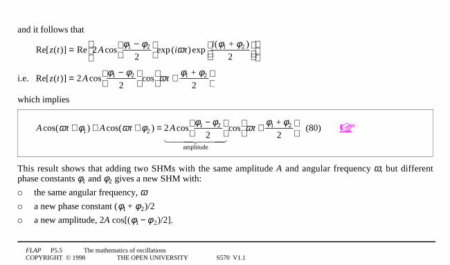
FLAP P5.5 The mathematics of oscillationsCOPYRIGHT © 1998 THE OPEN UNIVERSITY S570 V1.1
and it follows that
Re[z(t)] = Re 2A cosφ1 − φ2
2
exp(iω t) exp
i(φ1 + φ2 )2
i.e. Re[z(t)] = 2A cosφ1 − φ2
2
cos ω t + φ1 + φ2
2
which implies
A cos(ω t + φ1) + A cos(ω t + φ2 ) = 2A cosφ1 − φ2
2
amplitude1 2444 3444
cos ω t + φ1 + φ2
2
(80)
This result shows that adding two SHMs with the same amplitude A and angular frequency ω, but differentphase constants φ1 and φ2 gives a new SHM with:
o the same angular frequency, ωo a new phase constant (φ1 + φ12)/2
o a new amplitude, 2A cos[(φ1 − φ12)/2].
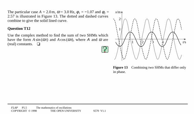
FLAP P5.5 The mathematics of oscillationsCOPYRIGHT © 1998 THE OPEN UNIVERSITY S570 V1.1
2
1
x/m
t/s4321
Figure 134Combining two SHMs that differ onlyin phase.
The particular case A = 2.01m, ω = 3.01Hz, φ1 = −1.07 and φ2 =2.57 is illustrated in Figure 13. The dotted and dashed curvescombine to give the solid lined curve.
Question T12
Use the complex method to find the sum of two SHMs whichhave the form A1sin1(ω1t) and A1cos1(ω1t), where Α and ω are(real) constants.4
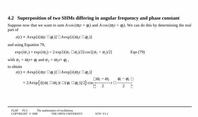
FLAP P5.5 The mathematics of oscillationsCOPYRIGHT © 1998 THE OPEN UNIVERSITY S570 V1.1
4.2 Superposition of two SHMs differing in angular frequency and phase constantSuppose now that we want to sum A1cos1(ω1t + φ1) and A1cos1(ω2t + φ2). We can do this by determining the realpart of
z(t) = A exp[i(ω1t + φ1)] + A exp[i(ω2t + φ2 )]
and using Equation 79,
exp1(iα 1) + exp1(iα2) = 21exp1[i(α1 + α2)/2]1cos1[(α1 − α2)/2] Eqn (79)
with α1 = ω01t+ φ1 and α 02 = ω12t+ φ2 ,
to obtainz(t) = A exp[i(ω1t + φ1)] + A exp[i(ω2t + φ2 )]
= 2A exp i[(ω1 + ω2 )t + (φ1 + φ2 )] 2 cosω1 − ω2
2t +
φ1 − φ2
2

FLAP P5.5 The mathematics of oscillationsCOPYRIGHT © 1998 THE OPEN UNIVERSITY S570 V1.1
Taking the real part we obtain
A1cos1(ω1t + φ1) + A1cos1(ω2t + φ2) = Re[z(t)]
= 2A cos(ω1 − ω2 )t + (φ1 − φ2 )
2
cos(ω1 + ω2 )t + (φ1 + φ2 )
2
(81)
This general expression is fairly complicated and so it is useful to consider a particular case as in the followingexercise.
Question T13
Use Equation 79
exp1(iα 1) + exp1(iα2) = 21exp1[i(α1 + α2)/2]1cos1[(α1 − α2)/2] Eqn (79)
to find the sum of two SHMs which have the form A1cos1(21ω1t + π/4) and A1cos1(23ω1t − π/4) where ω and A arereal constants. Sketch the resulting function of t and comment on the form of your result.4

FLAP P5.5 The mathematics of oscillationsCOPYRIGHT © 1998 THE OPEN UNIVERSITY S570 V1.1
4.3 Superposition of many SHMs1—1the diffraction grating
S1
S2
d θθ
D
O
Pscreen
N
Figure 144A diffraction grating.
Finally, we consider a problem that is of considerable importance in thestudy of optics. This concerns the pattern of illumination created on adistant screen when a uniform beam of light of a single colourencounters a diffraction grating. For our present purposes a diffractiongrating may be thought of as consisting of a large number of narrowparallel slits, each of which acts as a source of light. Two of these slits,S1 and S2, together with the screen are indicated in Figure 14, thoughthe figure has not been drawn to scale (D should be so much larger thand that the lines S1P and S2P are effectively parallel).
As explained elsewhere in FLAP, light may often be treated as a wavephenomenon; so at a given point P on the screen, the effect of the lightspreading out from each of the slits is to create an oscillation that maybe represented by a1cos1(ω1t + φ), where the angular frequency of theoscillation is determined by the colour of the light, and the phaseconstant φ is determined by the distance between the relevant slit andthe point P.
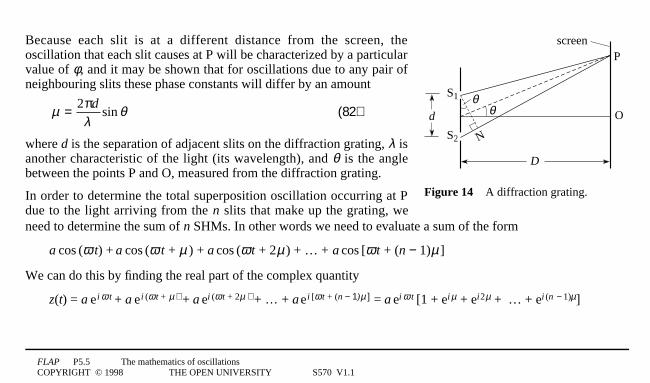
FLAP P5.5 The mathematics of oscillationsCOPYRIGHT © 1998 THE OPEN UNIVERSITY S570 V1.1
S1
S2
d θθ
D
O
Pscreen
N
Figure 144A diffraction grating.
Because each slit is at a different distance from the screen, theoscillation that each slit causes at P will be characterized by a particularvalue of φ, and it may be shown that for oscillations due to any pair ofneighbouring slits these phase constants will differ by an amount
µ = 2πd
λsin θ (82)
where d is the separation of adjacent slits on the diffraction grating, λ isanother characteristic of the light (its wavelength), and θ is the anglebetween the points P and O, measured from the diffraction grating.
In order to determine the total superposition oscillation occurring at Pdue to the light arriving from the n slits that make up the grating, weneed to determine the sum of n SHMs. In other words we need to evaluate a sum of the form
a1cos1(ω1t) + a1cos1(ω1t + µ1) + a1cos1(ω1t + 2µ1) + … + a1cos1[ω1t + (n − 1)µ1]
We can do this by finding the real part of the complex quantity
z(t) = a1e0i1ω1t + a1e0i1(ω1t + µ1) + a1ei1(ω1t + 2µ1) + … + a1e0i1[ω1t + (n − 1)µ1] = a1ei1ω1t [1 + ei1µ + ei12µ + … + ei1(n − 1)µ]

FLAP P5.5 The mathematics of oscillationsCOPYRIGHT © 1998 THE OPEN UNIVERSITY S570 V1.1
z(t) = a1e0i1ω1t + a1e0i1(ω1t + µ1) + a1ei1(ω1t + 2µ1) + … + a1e0i1[ω1t + (n − 1)µ1] = a1ei1ω1t [1 + ei1µ + ei12µ + … + ei1(n − 1)µ]
The sum in the square brackets is a geometric series with first term 1, and common ratio ei0µ and(from Question R5) this can be written as
1 + eiµ + ei2µ + … + ei(n−1)µ = 1 − einµ
1 − eiµ (83)
and the resulting expression for z(t) is
z(t) = a eiω t 1 − einµ
1 − eiµ
The terms involving µ can be rearranged as follows
1 − einµ
1 − eiµ = einµ / 2
eiµ / 2
einµ / 2 − e− inµ / 2
eiµ / 2 − e− iµ / 2
=einµ / 2 sin nµ 2( )eiµ / 2 sin µ 2( ) (84)
Substituting this in the expression for z(t) and taking the real part gives
Re[z(t)] = asin(nµ 2)sin(µ 2)
cos ω t + (n − 1)µ2

FLAP P5.5 The mathematics of oscillationsCOPYRIGHT © 1998 THE OPEN UNIVERSITY S570 V1.1
We can see from this result that:
o the angular frequency is ω;
o the phase constant is (n − 1)µ
2;
o the amplitude, A say, is given by
A = asin(nµ 2)sin(µ 2)
(85)
Substituting the value of µ from Equation 82
µ = 2πd
λsin θ (Eqn 82)
we can write this as
A = asin[nπd sin(θ ) λ ]sin[πd sin(θ ) λ ]
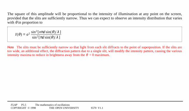
FLAP P5.5 The mathematics of oscillationsCOPYRIGHT © 1998 THE OPEN UNIVERSITY S570 V1.1
The square of this amplitude will be proportional to the intensity of illumination at any point on the screen,provided that the slits are sufficiently narrow. Thus we can expect to observe an intensity distribution that varieswith θ in proportion to
I(θ ) = a2 sin2[nπd sin(θ ) λ ]sin2[πd sin(θ ) λ ]
Note The slits must be sufficiently narrow so that light from each slit diffracts to the point of superposition. If the slits aretoo wide, an additional effect, the diffraction pattern due to a single slit, will modify the intensity pattern, causing the variousintensity maxima to reduce in brightness away from the θ = 0 maximum.
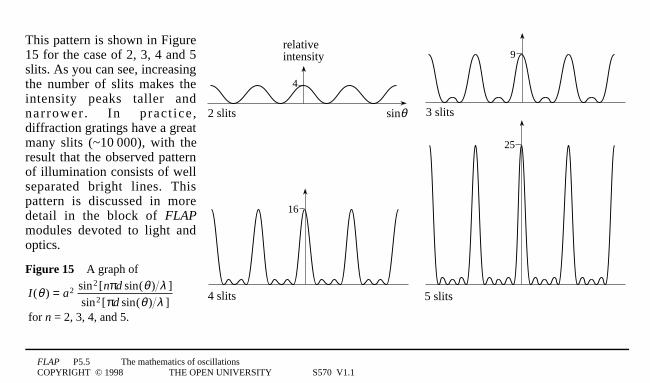
FLAP P5.5 The mathematics of oscillationsCOPYRIGHT © 1998 THE OPEN UNIVERSITY S570 V1.1
2 slits
relativeintensity
4
9
3 slits
4 slits
16
5 slits
25
sinθ
This pattern is shown in Figure15 for the case of 2, 3, 4 and 5slits. As you can see, increasingthe number of slits makes theintensity peaks taller andnarrower . In pract ice ,diffraction gratings have a greatmany slits (~101000), with theresult that the observed patternof illumination consists of wellseparated bright lines. Thispattern is discussed in moredetail in the block of FLAPmodules devoted to light andoptics.
Figure 154A graph of
I(θ ) = a2 sin2 [nπd sin(θ ) λ ]
sin2 [πd sin(θ ) λ ] for n = 2, 3, 4, and 5.
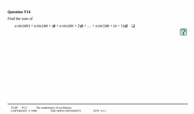
FLAP P5.5 The mathematics of oscillationsCOPYRIGHT © 1998 THE OPEN UNIVERSITY S570 V1.1
Question T14
Find the sum of
a1sin1(ω1t) + a1sin1(ω1t + φ) + a1sin1(ω1t + 2φ) + … + a1sin1[ω1t + (n − 1)φ]4

FLAP P5.5 The mathematics of oscillationsCOPYRIGHT © 1998 THE OPEN UNIVERSITY S570 V1.1
5 Closing items
5.1 Module summary1 Differential equations of second order with constant coefficients arise from many physical situations, in
particular: mechanical and electrical systems.
A mass m subject to a sinusoidal driving force F(t) = F01sin1(Ω1t), a damping force proportional to velocityand a restoring force proportional to displacement from the origin, will satisfy a differential equation of theform
md2 x(t)
dt2+ b
dx(t)dt
+ kx(t) = F0 sin (Ω t) (Eqn 13)
The charge q(t) on a capacitor in a series LCR circuit containing a resistance R, a capacitance C and aninductance L, subject to an externally applied voltage V(t) = V01sin1(Ω1t), will satisfy a similar differentialequation
Ld2q(t)
dt2+ R
dq(t)dt
+ 1C
q(t) = V0 sin (Ω t) (Eqn 17)
Both equations give rise to harmonically driven, linearly damped harmonic oscillations.
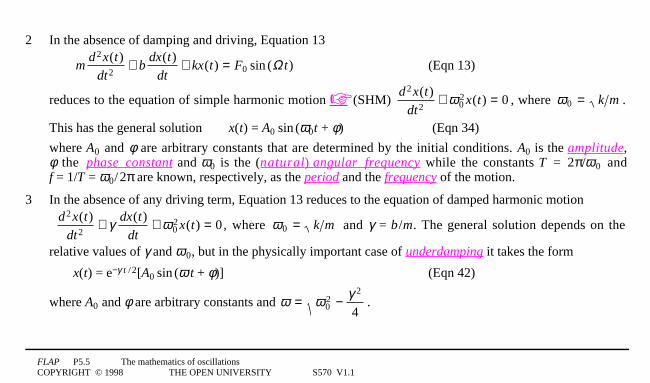
FLAP P5.5 The mathematics of oscillationsCOPYRIGHT © 1998 THE OPEN UNIVERSITY S570 V1.1
2 In the absence of damping and driving, Equation 13
md2 x(t)
dt2+ b
dx(t)dt
+ kx(t) = F0 sin (Ω t) (Eqn 13)
reduces to the equation of simple harmonic motion (SHM) d2 x(t)
dt2+ ω0
2 x(t) = 0 , where ω0 = k m .
This has the general solution x(t) = A01sin1(ω0t + φ) (Eqn 34)
where A0 and φ are arbitrary constants that are determined by the initial conditions. A0 is the amplitude,φ the phase constant and ω0 is the (natural) angular frequency while the constants T = 2π/ω00 andf = 1/T = ω00/02π are known, respectively, as the period and the frequency of the motion.
3 In the absence of any driving term, Equation 13 reduces to the equation of damped harmonic motion
d2 x(t)
dt2+ γ dx(t)
dt+ ω0
2 x(t) = 0 , where ω0 = k m and γ = b/m. The general solution depends on the
relative values of γ and ω00, but in the physically important case of underdamping it takes the form
x(t) = e−γ t /12[A01sin1(ω1t + φ)] (Eqn 42)
where A0 and φ are arbitrary constants and ω = ω02 − γ 2
4.
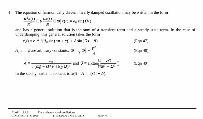
FLAP P5.5 The mathematics of oscillationsCOPYRIGHT © 1998 THE OPEN UNIVERSITY S570 V1.1
4 The equation of harmonically driven linearly damped oscillation may be written in the form
d2 x(t)dt2
+ γ dx(t)dt
+ ω02 x(t) = a0 sin (Ω t)
and has a general solution that is the sum of a transient term and a steady state term. In the case ofunderdamping, this general solution takes the form
x(t) = e−γ1t1/12[A01sin1(ω1t + φ)] + A1sin1(Ω1t − δ1) (Eqn 47)
A0 and φ are arbitrary constants, ω = ω02 − γ 2
4(Eqn 48)
A = a0
(ω02 − Ω 2 )2 + (γ Ω )2
and δ = arctanγ Ω
ω02 − Ω 2
(Eqn 49)
In the steady state this reduces to x(t) = A1sin1(Ω1t − δ1).

FLAP P5.5 The mathematics of oscillationsCOPYRIGHT © 1998 THE OPEN UNIVERSITY S570 V1.1
5 When a voltage V(t) = V01sin1(Ω1t) is applied across a series LCR circuit, the resulting steady state currenthas the form I(t) = I01sin1(Ω11t − δ1)where V0 = I0Z4and4δ = arctan1(X/R)
Z being the impedance given by
Z = R2 + X2 and X = XL − XC = Ω1L − 1/(Ω1C) the total reactance.
6 In the case of the mechanical system described by Equation 13 the mechanical impedance is defined by Zm
= F0/v0 where v0 is the amplitude of the velocity oscillation and Zm = b2 + k
Ω− Ω m
2
.
7 Resonance is the phenomenon whereby a driven oscillator exhibits large amplitude oscillations when drivenat a frequency close to the natural frequency it would have in the absence of any driving or damping.
8 When analysing a.c. circuits in their steady state, it is convenient to represent the applied voltage V(t) as thereal part of a complex quantity V1(t) =V01e0i1ω1t and the current I(t) as the real part of a complex quantity ((t)= (01e0i1ω1t, where V0 and (0 are complex constants. The complex form of Ohm’s law is then the equationV(t) = ((t) Z where Z is the complex impedance. The value Z = |1Z1| is the impedance, and δ = arg(Z) is theextent by which the phase of the current lags behind that of the driving voltage.

FLAP P5.5 The mathematics of oscillationsCOPYRIGHT © 1998 THE OPEN UNIVERSITY S570 V1.1
9 For complex impedances combined in series
Z = Z01 + Z02 + … Z0n (Eqn 73)
For complex impedances combined in parallel
1Z
= 1Z1
+ 1Z2
+ … + 1Zn
(Eqn 74)
For a single resistor, ZR = R, for a single capacitor ZC = 1/(iω1C), and for a single inductor ZL = iω1L.
10 The average power dissipated by a circuit carrying alternating current is
⟨P⟩ = 1
2Re(( 0
*V 0 ) (Eqn 78)
11 The effect of superposing harmonic oscillations may be found by adding together appropriate complexquantities and then taking the real part of the result (or the imaginary part if appropriate).

FLAP P5.5 The mathematics of oscillationsCOPYRIGHT © 1998 THE OPEN UNIVERSITY S570 V1.1
5.2 AchievementsHaving completed this module, you should be able to:
A1 Define the terms that are emboldened and flagged in the margins of the module.
A2 Use second-order differential equations to model a variety of oscillatory problems and to highlight theanalogy between mechanical and electrical systems in situations where both are modelled by similardifferential equations.
A3 To explain the significance of impedance and resonance in relation to the amplitude of the steady statesolution to the sinusoidally driven, linearly damped harmonic oscillator.
A4 Use complex numbers to solve simple problems involving LCR circuits and to display relative magnitudesand phases of currents and voltages by means of an Argand diagram.
A5 To calculate the average power dissipated by a suitable component in a simple a.c. circuit.
A6 Use complex numbers to solve problems involving SHM, including the superposition of two or moreSHMs.
Study comment You may now wish to take the Exit test for this module which tests these Achievements.If you prefer to study the module further before taking this test then return to the Module contents to review some of thetopics.

FLAP P5.5 The mathematics of oscillationsCOPYRIGHT © 1998 THE OPEN UNIVERSITY S570 V1.1
5.3 Exit testStudy comment Having completed this module, you should be able to answer the following questions each of which testsone or more of the Achievements.
Question E1
(A2)4The general solution of the differential equation
d2 x(t)dt2
+ 2qω dx(t)dt
+ (n2 + q2 )ω 2 x(t) = 0
is x(t) = e−qω t [A cos(nω t) + Bsin (nω t)]
and a particular solution of the differential equation
d2 x(t)dt2
+ 2qω dx(t)dt
+ (n2 + q2 )ω 2 x(t) = h sin (Ω t)
is xp (t) = c cos(Ω t) + d sin (Ω t)
where c = − 2qωΩ h H 4and4 d = [(q2 + n2 )ω 2 − Ω 2 ]h H
with H = q4ω 2 + 2q2ω 2 (n2 + 1) + (n2ω 2 − Ω 2 )2 and n ≠ Ω /ω.
FLAP P5.5 The mathematics of oscillationsCOPYRIGHT © 1998 THE OPEN UNIVERSITY S570 V1.1
Use this solution to write down the transient current and the steady state current in a series LCR circuitcontaining a resistor 61Ω, a capacitor 1/131F and an inductor 11H, when it is driven by an applied voltageV(t) = V01cos1(Ω1t + π), where V0 = 1.001V and Ω = 1.001s−1. Describe an analogous mechanical system.
Question E2
(A2)4What is the resonant frequency of the electrical circuit described in Question E1? What would you expectto happen when the angular frequency of the applied voltage is close to this value?
Question E3
(A4 and A5)4Calculate the complex impedance of a resistance 61Ω, a capacitor 1/131F and an inductor 11H inseries. What is the current through the circuit if a voltage V(t) = V01cos1(ω1t + π), where ω = 11s−1, is applied tothe circuit? Sketch the complex current and voltage on an Argand diagram, and calculate the average powerdissipated.
FLAP P5.5 The mathematics of oscillationsCOPYRIGHT © 1998 THE OPEN UNIVERSITY S570 V1.1
Question E4
(A6)4Use a complex representation to find the result of adding two SHMs of the form a1sin1(ω1t − kx) anda1sin1(2ω1t + 2kx).
Study comment This is the final Exit test question. When you have completed the Exit test go back to Subsection 1.2 andtry the Fast track questions if you have not already done so.
If you have completed both the Fast track questions and the Exit test, then you have finished the module and may leave ithere.