Fleet Fatality Risk Sensitivity to

Vehicle Mass/Size Change in Vehicle-to-Vehicle Crashes

Guy S. Nusholtz and Yibing Shi Chrysler Group LLC

Combined Empirical and Theoretical Modeling Parameterized Accident and other Data to form basis for a set of equations. Include the laws of physics.

—A fleet model is creAted Different from building the model from the crashing of computational cars such as in FEA

Input

Mass distribution data (5,262 vehicles) from F-F crashes from FARS [Kahane 2012]

0 2000 4000 6000 80000

0.05

0.1

0.15

0.2

Vehicle mass (lb)

Freq

uenc

y

Field dataGamma fit

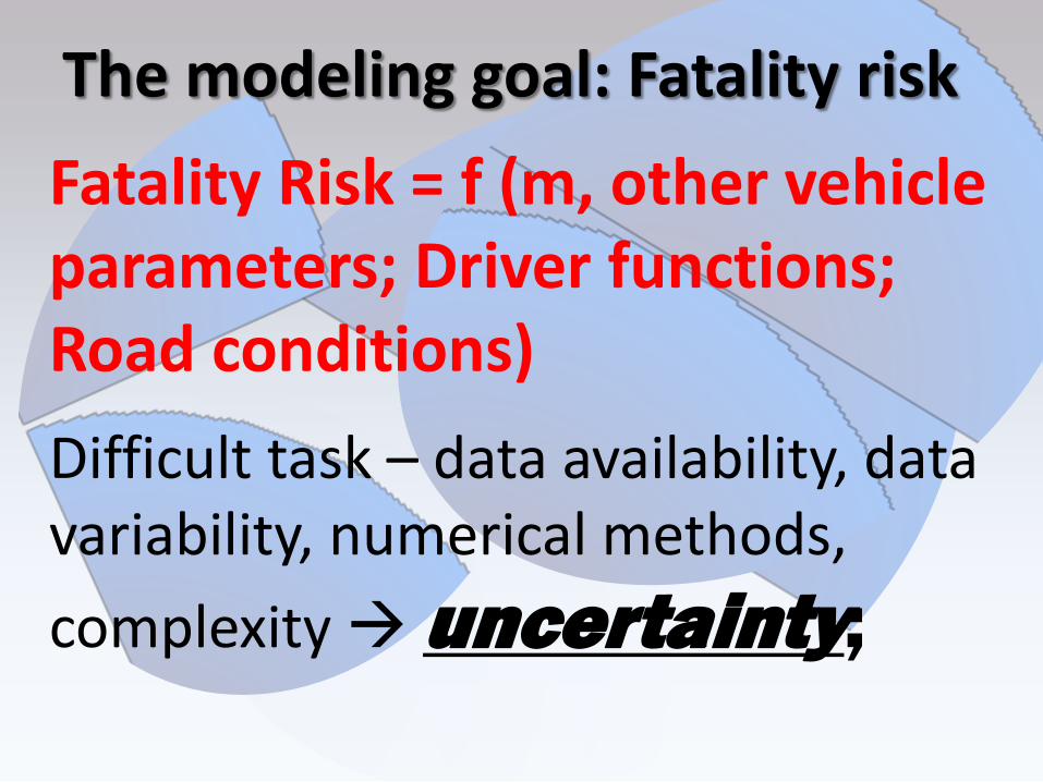
The modeling goal: Fatality risk Fatality Risk = f (m, other vehicle parameters; Driver functions; Road conditions) Difficult task – data availability, data variability, numerical methods, complexity uncertainty;

Background -- 2

Joksch Mass ( 93) Evans, et. al. Mass; Risk ratio(92)

Kahane Fatality Rate multi-regression models (‘97, ‘03, ’12) van Auken et. al. Fatality Rate multi-regression models (’02 - ’12) Padamanaban Fatality Rate multi-regression models (03-09) Shi and Nusholtz Fatality Rate multi-regression models (13)

Model Development (1) Fatality Risk Empirical Model (EM1)

𝒓 = 𝒗𝒗𝟎𝟎

𝒂

α 3.88 +- 0.19 𝒗𝟎𝟎 (mph) 70.6

(2) Fatality Risk Ratio Empirical Models-vehicle-vehicle crashes (EM2); 𝒓𝟏𝒓𝟐

=𝒎𝟐

𝒎𝟏

𝜷

[Evans 1992, etc.]

[Joksch 1993]

β 3.36;

3.58; 3.73

𝐥𝐥𝒓𝟏𝒓𝟐

= −𝟑.𝟖𝟑 𝐥𝐥𝒎𝟏

𝒎𝟐− 𝟎.𝟑𝟏𝑫𝑽𝑽𝑽𝑽𝑽𝒓𝑽𝑽𝑽 − 𝟎.𝟑𝟑𝑫𝑽𝑽𝑽𝑽𝑽𝑽𝒗

− 𝟎.𝟑𝟑𝑫𝑽𝑽𝑽𝑽𝑽𝑽𝒗 − 𝟎.𝟑𝟑𝑫𝑬𝑬𝑬 − 𝟏.𝟐𝟎𝑫𝑹𝑬𝑬𝑽_𝑼𝑬𝑬+ 𝟎.𝟎𝟎𝑫𝑨𝟏𝟑−𝟑𝟎 + 𝟎.𝟎𝟑𝑫𝑨𝟑𝟖−𝟔𝟎 + 𝟎.𝟎𝟎𝑫𝑨𝟔𝟎−𝟗𝟎

[Shi & Nusholtz 2013] (3) r = f(m; VTYP, age, rest use; ….) ?

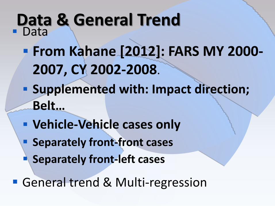
Data & General Trend Data From Kahane [2012]: FARS MY 2000-

2007, CY 2002-2008. Supplemented with: Impact direction;

Belt… Vehicle-Vehicle cases only Separately front-front cases Separately front-left cases

General trend & Multi-regression

Data & General Trend

Front-front crashes. Conditional fatality risk.

0 2000 4000 6000 80000

0.2

0.4

0.6

0.8

1

Vehicle mass (lb)

Con

ditio

n Fa

talit

y R

isk

Data & General Trend

Front-front crashes. Conditional fatality risk.

0 20 40 60 80 1000

0.2

0.4

0.6

0.8

1

Age (years)

Cond

itiona

l Risk

Belted

Unbelted

Risk Ratio -- aggregated

Front-front crashes

0 0.2 0.4 0.6 0.8 1 1.2-5

-4

-3

-2

-1

0

1

ln(mass ratio)

ln(r

isk r

atio)

Aggregated dataln(rr) = 0.14-4.57*ln(ρ)

0 0.5 1 1.5-5

-4

-3

-2

-1

0

ln(mass ratio)

ln(r

isk r

atio

)

Aggregated dataln(rr) = 0.06-4.13*ln(ρ)Weighted ln(rr) = 0.03-4.04*ln(ρ)

-1 -0.5 0 0.5 1-6

-5

-4

-3

-2

-1

0

1

ln(mass ratio)

ln(r

isk r

atio)

Aggregated dataln(rr) = -2.17-3.47*ln(ρ)

Risk Ratio -- aggregated

Front-Left crashes

-1 -0.5 0 0.5 1 1.5-6

-4

-2

0

2

4

ln(mass ratio)

ln(r

isk r

atio)

Aggregated dataln(rr) = -2.06-3.6*ln(ρ)Weighted ln(rr) = -2.09-3.65*ln(ρ)

0 10 20 30 40 50 600

0.1

0.2

0.3

0.4

0.5

0.6

Velocity (mph)

Ris

k

Power function: α = 3.83, vop = 70 mph

Logistic function: β = 4.17, vol = 63.03 mph

Discussion: Uncertainty with Risk Function

𝑟 = 1

1 + 𝑣𝑣0𝑙

−𝐵

𝑟 = 𝑣𝑣0𝑝

𝑎

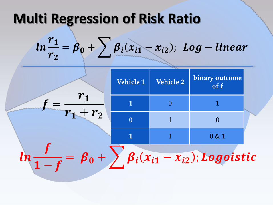
Multi Regression of Risk Ratio

𝒍𝒍𝒓𝟏𝒓𝟐

= 𝜷𝟎 + �𝜷𝒊 𝒙𝒊𝟏 − 𝒙𝒊𝟐 ; 𝑳𝑳𝑳 − 𝒍𝒊𝒍𝒍𝒂𝒓

𝒇 =𝒓𝟏

𝒓𝟏 + 𝒓𝟐

𝒍𝒍𝒇

𝟏 − 𝒇= 𝜷𝟎 + �𝜷𝒊 𝒙𝒊𝟏 − 𝒙𝒊𝟐 ;𝑳𝑳𝑳𝑳𝒊𝑽𝑽𝒊𝑽

Vehicle 1 Vehicle 2 binary outcome of f

1 0 1

0 1 0

1 1 0 & 1

Stability of Regression Result

CURBWT VTYPtruck VTYPsuv VTYPcuv ESC REST_USE

-5.000 -4.500 -4.000 -3.500 -3.000 -2.500 -2.000 -1.500 -1.000 -0.500 0.000

991 pairs 2008 pairs 2206 pairs

F-F Crashes

Stability of Regression Result

0.000

0.010

0.020

0.030

0.040

0.050

0.060

0.070

0.080

A14_30 A38_60 A60_96

991 pairs2008 pairs2206 pairs

F-F Crashes

Application: from ratio to risk

0.5 1 1.5 20

0.5

1

1.5

2

2.5

3

Normalized subject vehicle mass

Nor

m. a

ve. s

ubje

ct v

ehile

risk

Numerical Integration1st order approximation2nd order approximation

Closing Velocity Distribution �̿�1 𝑚1 = 𝑘�

1

1 + ∆2𝑣0𝑝

𝜇 2𝑚2𝑚1 + 𝑚2

𝜇 𝑝∆ ∆ ∙ 𝑝𝑚 𝑚2 𝑑∆𝑑𝑚2

0 20 40 60 80 1000

0.01

0.02

0.03

0.04

0.05

0.06

Closing velocity ∆ (mph)

Pro

babi

lity

dens

ity (1

/mph

)

p∆1(∆): µ∆ = 25.56 mph, σ∆ = 7.80 mph

p∆2(∆): µ∆ = 51.12 mph, σ∆ = 11.03 mph

Fleet Risk Sensitivity to Risk Function (and Closing Velocity Distribution)

Risk increase per 100 lb of decrease in subject vehicle mass

2000 3000 4000 5000 6000-2

0

2

4

6

Case vehicle mass (lb)

Incr

ease

in s

ocita

l ris

k (%

)

Power risk functionLogistic risk function with p∆1

Logistic risk function with p∆2

Discussion: Mass vs. length

SAE 2013-01-0466

0.5 1 1.5 20

0.2

0.4

0.6

0.8

(m1+m2)/2/mµ or (L1

2.45 + L22.45)/2/L

µ2..45

Co

nditio

na

l R

isk

-1.5 -1 -0.5 0 0.5 1 1.50

0.2

0.4

0.6

0.8

1

ln(m1/m2) or 2.45*ln(L1/L2)

Co

nditio

na

l R

isk

20

Effect of Mass on Velocity Change

)( 2121

21 vv

mmmv ++

=∆ )( 2121

12 vv

mmmv ++

=∆

. 8.20 , 2.29 , 50 and , 3500 , 2500For

21

2121

mphvmphvmphvvlbmlbm

=∆=∆

=+==

m1 m2 v1 v2

0

10

20

30

40

50

Log (massratio)

StruckDriver Age

StrikingVehicleFAW

StruckAirbag

Deployed

StruckVehicle Age

StruckDriver

Drinking

Striking LogStiff. (Ke2)x Bumper

Ht.

Pe

rce

nt o

f To

tal C

on

trib

utio

nRelative Contribution of Variables

to Odds of Fatality Car-to-Car, Frontal Crashes

Mass is the dominant vehicle factor in

car-to-car crashes

21

02468

101214161820

15 20 25 30 35 40 45 50 55

Perc

enta

ge of

fata

litie

s

Delta V (mph)

r1: lighter carDelta V1 =29.2

r2: heavier carDelta V2=20.8

Effect of Velocity Change on Fatality

22

Ratio of fatality risk ~ 4%/1.5%=2.7 Occupants in the lighter vehicle are at

2.7 times greater risk

Source: Evans 2000

Example of Kahane [2012] Analysis Result

Crash Type Point estimate (%) 95% Confidence bounds (%)

Lower Upper

1st-event Rollover -2.16 -4.65 0.33 Hit fixed object -0.68 -2.40 1.05 Hit pedestrian/bike/motorcycle 1.95 0.07 3.84 Hit heavy vehicle 2.14 -1.26 5.54 Hit car-CUV-minivan < 3,082 lb 0.68 -1.61 2.98 Hit car-CUV-minivan > 3,082 lb 0.37 -2.44 3.17 Hit truck-based LTV < 4,150 lb 1.10 -1.98 4.18 Hit truck-based LTV > 4,150 lb 5.97 3.18 8.76 All others 1.85 -0.38 4.08

100-lb Mass Reduction Cars < 3,106 lb, Holding Footprint Constant

V-V Crashes: [EM1 Conservation of Momentum EM2 ] r(m; …)

𝑣1 = 𝑚2𝑚1+𝑚2

∆ & 𝑣2 = 𝑚1𝑚1+𝑚2

∆ CE + Fully plastic:

Sub. into EM1: 𝑟1 = 2𝑚2𝑚1+𝑚2

𝛼 ∆2𝑣0𝑝

𝛼 & 𝑟2 = 2𝑚1

𝑚1+𝑚2

𝛼 ∆2𝑣0𝑝

𝛼

𝑟1𝑟2

=𝑚2

𝑚1

𝑎

𝑟1𝑟2

= 𝑘𝐷𝑉𝑉𝑉𝑉 ∙ 𝑘𝐷𝐸𝐸𝐸 ∙ 𝑘𝐷𝐵𝐵𝐵𝐵 ∙ 𝑘𝐷𝐴𝐴𝐵𝑚2

𝑚1

𝛽

𝑟1(𝑚1,𝑚2,∆;𝛽, 𝑣0𝑝; … ) = 𝑘𝐷2𝑚2

𝑚1+𝑚2

𝛽 ∆2𝑣0𝑝

𝛽

Form from EM1; mass brought in with Conservation of momentum; β (& other effects) from EM2.

Fleet average risk

�̿�1 𝑚1 = 𝑘∬ ∆2𝑣0𝑝

𝛼 2𝑚2𝑚1+𝑚2

𝛼𝑝∆ ∆ 𝑝𝑚 𝑚2 𝑑∆𝑑𝑚2

= 𝑘𝐶 ∙ ∫ 2𝑚2𝑚1+𝑚2

𝛼𝑝𝑚 𝑚2 𝑑𝑚2

Averaged over crash vel. dist. & other vehicle mass -> subject vehicle Ave. Risk

Sum of two vehicles “societal risk” �̿� 𝑚1 ≜ �̿�1 𝑚1 + �̿�2 𝑚1

= 𝐶�2𝑚1

𝑚1 + 𝑚2

𝛼

+2𝑚2

𝑚1 + 𝑚2

𝛼

𝑝𝑚 𝑚2 𝑑𝑚2

Next: Evaluate with given pm(m); compare with Kahane result

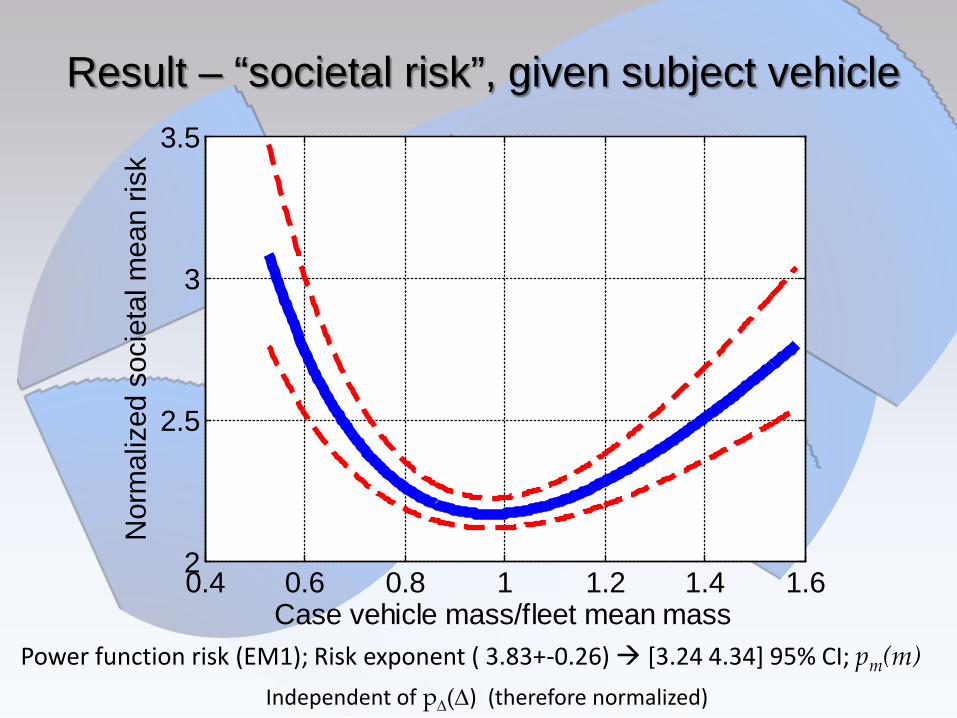
Result – “societal risk”, given subject vehicle

Power function risk (EM1); Risk exponent ( 3.83+-0.26) [3.24 4.34] 95% CI; pm(m) Independent of p∆(∆) (therefore normalized)

0.4 0.6 0.8 1 1.2 1.4 1.62

2.5

3

3.5

Case vehicle mass/fleet mean mass

Nor

mal

ized

soc

ieta

l mea

n ris

k

Reduction of Kahane Result Kahane result mainly used in the context of:

Percent increase in societal fatality rate per 100 lb decrease in subject vehicle mass

𝑅𝑅𝑅(𝑚) ≜1

�̿� 𝑚𝑑�̿� 𝑚𝑑𝑚

�̿� 𝑚 = 𝐶 �2𝑚

𝑚 + 𝑚𝑜

𝛼

+2𝑚𝑜

𝑚 + 𝑚𝑜

𝛼

𝑝𝑚 𝑚𝑜 𝑑𝑚𝑜

“Relative Rate of change of societal Risk for subject vehicle of mass m

Comparison

Increase in societal risk for 100 lb case vehicle mass reduction

2000 3000 4000 5000 6000-4

-2

0

2

4

6

Case vehicle mass (lb)

Incr

ease

in s

ocita

l ris

k (%

)

Cars >= 3,106 lb

Cars < 3,106 lb

Pickups & SUVs >= 4,594 lb

CUVs & Minivans

Pickups & SUVs < 4,594 lb

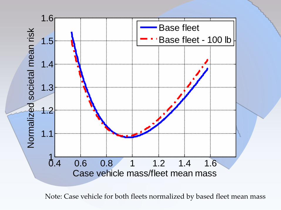
Note: Case vehicle for both fleets normalized by based fleet mean mass

0.4 0.6 0.8 1 1.2 1.4 1.61

1.1

1.2

1.3

1.4

1.5

1.6

Case vehicle mass/fleet mean mass

Nor

mal

ized

soc

ieta

l mea

n ris

k

Base fleetBase fleet - 100 lb

0 50 100 150 200 250 3000

0.5

1

1.5

2

2.5

3

3.5

Mass reduction (lb)

Incr

ease

in m

ean

fleet

risk

(%)

α= 3.83

(Upper 95% from regression)

(lower 95% from regression)

Summary & Conclusions --1

• A fleet fatality risk model has been established (again). Assuming • Conservation of momentum, energy • r(v) empirical relationship( accident data) • Current distribution of vehicle parameters

• Then • Model societal risk change due to mass

change comparable to Kahane 2012 result • Consistent r1/r2 v.s. m1/m2 (accident data)

Summary & Conclusions -- 2

• Kahane’s result appears to be in essence a manifestation of the two relationships: velocity (risk) and C.M.

• Model uncertainty examined via risk exponent; risk functional form (& velocity distribution); Result: model is stable.

• For the observed variation mass has a greater effect on risk than other parameters, such as stiffness, crush, wheel base..etc.

Summary & Conclusions -- 2 For Front-Front crashes:

Mass ratio risk exponent ~ 3.8 Consistent with existing data. Reflection of conservation of momentum and velocity risk

Belted: ~0.3x relative to unbelted

10-years age increase above the 30-38 year range (lowest fatality risk): ~ 1.5x

Summary & Conclusions -- 3

For Front-Left crashes: R_bullet: R_target ~= 1:8, when all other parameters are equal. Mass ratio risk exponent ~= 4.2, slightly larger Driver age was found to influence driver fatality risk

Summary & Conclusions -- 4

The effect of Mass on societal risk: Risk from Crash velocity Conservation of Momentum Parameter distribution: mass, stiffness, available, size crush…etc. Dictates results

The regression result may be used to model risk.

Acknowledgements The authors would like to thank: Dr. Charles Kahane of NHTSA for providing

and explaining the FARS data set Ms. Fariba Famili of Chrysler Group LLC and

Mr. Charlie Campton of UMTRI for providing the supplemental information on the FARS data Ms. Jeya Padamanaban for all the

analysis she has generated over time Dr. Jianping Wu of Chrysler Group LLC for

his insights