flavor changing neutra...to discriminate between 2hdm and supersymmetric higgs bosons. furthermore,...
TRANSCRIPT

Departament de FísicaUniversitat Autònoma de Barcelona
Grup de Física Teòrica
Flavor changing neutral decayeffects in models with
two Higgs boson doublets:Applications to LHC Physics.
Efectes de decaıments amb canvi de sabor neutres
en models amb dos doblets de bosons de Higgs:
Aplicacions a la Fısica de LHC.
Santi Bejar Latonda
Universitat Autonoma de Barcelona
Grup de Fısica Teorica
Institut de Fısica d’Altes Energies
2005/2006
Memoria presentada per a optar al grau de
Doctor en Ciencies Fısiques
Director:
Dr. Joan Sola i Peracaula
Vull agrair a en Joan Sola la seva gran dedicacio, sense el qual aquest treball no hauria
estat possible. Per la seva confianca en el meu saber fer, tant en la feina com en el temps
de compilar el resultat final. Ha estat comprensiu i un gran guia en els moments de dubte.
La seva visio sobre quins temes eren interessants estudiar de entre tots els camins que hi
ha en aquest camp i entre els que ben segur m’hauria perdut.
A en Jaume Guasch, un company infatigable i constant, disposat a resoldre dubtes i
a prendre un cafe quan ho necessitava. A mes li he d’agrair que m’acollıs com a un amic
al seu despatx tant de temps sense queixar-se. I per tot el treball que hem fet junts.
Al companys del Grup de Fısica Teorica els hi he d’agrair l’entorn que m’ha permes
seguir treballant en el camp que m’agrada i no haver perdut l’entusiasme. El treballar dia
a dia amb aquests fısics ha estat molt enriquidor. Las seves xerrades sobre fısica, sobre
els fısics, temes mundans i no tant mundans m’han ajudat a seguir treballant amb illusio
a la fısica.
Al Grup de Fısica Teorica per haver-me acollit proporcionat tots els medis necessaris
per poder treballar.
A la Ma del Carmen per escoltar i intentar entendre les meves divagacions, les meves
explicacions, tot i que la son es mes forta de vegades. Espero haver-te transmes una
miqueta de la meva passio per la fısica.
A la famılia i amics per comprendre que el ser fısic teoric no es nomes una excusa per
estar assegut dient que estas meditant sobre partıcules fonamentals, o l’origen de l’univers,
en lloc de parar la taula.
This Thesis has been written using Free Software.
The LATEX2ε Typesetting system.
Feynman graphs using feynMF.
Plots using Xmgr and Grace plotting tools.
GNU Emacs.
Running in a GNU/Linux system.
Contents
1 Introduction 1
1.1 Summary . . . . . . . . . . . . . . . . . . . . . . . . . . . . . . . . . . . . 1
1.2 Motivation . . . . . . . . . . . . . . . . . . . . . . . . . . . . . . . . . . . . 3
1.3 Today’s situation . . . . . . . . . . . . . . . . . . . . . . . . . . . . . . . . 5
2 Two Higgs Doublet Models (2HDM) 13
2.1 Introduction . . . . . . . . . . . . . . . . . . . . . . . . . . . . . . . . . . . 13
2.1.1 2HDM I . . . . . . . . . . . . . . . . . . . . . . . . . . . . . . . . . 15
2.1.2 2HDM II . . . . . . . . . . . . . . . . . . . . . . . . . . . . . . . . . 15
2.1.3 2HDM III . . . . . . . . . . . . . . . . . . . . . . . . . . . . . . . . 16
2.2 2HDM spectrum . . . . . . . . . . . . . . . . . . . . . . . . . . . . . . . . 16
2.2.1 Higgs sector . . . . . . . . . . . . . . . . . . . . . . . . . . . . . . . 16
2.3 Interactions in the mass-eigenstate basis . . . . . . . . . . . . . . . . . . . 18
2.4 Constraints . . . . . . . . . . . . . . . . . . . . . . . . . . . . . . . . . . . 20
3 The Minimal Supersymmetric Standard Model (MSSM) 23
3.1 Introduction . . . . . . . . . . . . . . . . . . . . . . . . . . . . . . . . . . . 23
3.2 Field content . . . . . . . . . . . . . . . . . . . . . . . . . . . . . . . . . . 26
3.3 Lagrangian . . . . . . . . . . . . . . . . . . . . . . . . . . . . . . . . . . . 27
3.4 MSSM spectrum . . . . . . . . . . . . . . . . . . . . . . . . . . . . . . . . 29
3.4.1 Higgs boson sector . . . . . . . . . . . . . . . . . . . . . . . . . . . 29
3.4.2 The SM sector . . . . . . . . . . . . . . . . . . . . . . . . . . . . . 32
3.4.3 Sfermion sector (Flavor-diagonal case) . . . . . . . . . . . . . . . . 33
3.4.4 Sfermion sector (Non-flavor-diagonal case) . . . . . . . . . . . . . . 34
3.5 Interactions in the mass-eigenstate basis . . . . . . . . . . . . . . . . . . . 35
3.6 Flavor changing neutral currents . . . . . . . . . . . . . . . . . . . . . . . . 37
3.7 MSSM parametrization . . . . . . . . . . . . . . . . . . . . . . . . . . . . . 42
3.7.1 MSSM parameters . . . . . . . . . . . . . . . . . . . . . . . . . . . 42
3.7.2 Constraints . . . . . . . . . . . . . . . . . . . . . . . . . . . . . . . 44
iii

4 Loop Induced FCNC Decays of the Top Quark in a General 2HDM 49
4.1 Introduction . . . . . . . . . . . . . . . . . . . . . . . . . . . . . . . . . . . 49
4.2 Relevant fields and interactions in the 2HDM . . . . . . . . . . . . . . . . 51
4.3 Numerical analysis . . . . . . . . . . . . . . . . . . . . . . . . . . . . . . . 52
4.4 Discussion and conclusions . . . . . . . . . . . . . . . . . . . . . . . . . . . 59
5 Higgs Boson FCNC Decays into Top Quark in a General 2HDM 65
5.1 Introduction . . . . . . . . . . . . . . . . . . . . . . . . . . . . . . . . . . . 65
5.2 Expected branching ratios in the SM and the 2HDM . . . . . . . . . . . . 66
5.3 Numerical analysis . . . . . . . . . . . . . . . . . . . . . . . . . . . . . . . 69
5.4 Discussion and conclusions . . . . . . . . . . . . . . . . . . . . . . . . . . . 84
6 Higgs Boson FCNC Decays into Bottom Quarks in the MSSM 87
6.1 Introduction . . . . . . . . . . . . . . . . . . . . . . . . . . . . . . . . . . . 87
6.2 Partial widths and branching ratios . . . . . . . . . . . . . . . . . . . . . . 89
6.3 Full one-loop SUSY-QCD calculation: Numerical analysis . . . . . . . . . . 91
6.4 Remarks and conclusions . . . . . . . . . . . . . . . . . . . . . . . . . . . . 102
7 Production and FCNC decay of MSSM Higgs bosons into heavy quarks
in the LHC 105
7.1 Introduction . . . . . . . . . . . . . . . . . . . . . . . . . . . . . . . . . . . 105
7.2 General setting for the numerical analysis . . . . . . . . . . . . . . . . . . . 107
7.3 Analysis of the bottom-strange channel . . . . . . . . . . . . . . . . . . . . 111
7.4 Analysis of the top-charm channel . . . . . . . . . . . . . . . . . . . . . . . 119
7.5 Discussion and conclusions . . . . . . . . . . . . . . . . . . . . . . . . . . . 123
8 Conclusions 129
A Vertex functions 133
A.1 Limit of heavy internal masses . . . . . . . . . . . . . . . . . . . . . . . . . 136
B Diagonalizing a squared mass matrix 139
List of Figures 143
List of Tables 147
Bibliography 149
iv

Chapter 1
Introduction
1.1 Summary
In this Thesis we have investigated some effects appearing in top quark and Higgs bo-
son decays with flavor changing neutral currents (FCNC) in the framework of generic
Two Higgs Doblet Models (2HDM) and the Minimal Supersymmetric Standard Model
(MSSM).
The Standard Model (SM) of Particle Physics interactions has had great success in
describing the strong, weak and electromagnetic interactions and its validity has been
tested up to the quantum level in past and present accelerators, such as the LEP at
CERN or the Tevatron at Fermilab. The last great success of the SM was the discovery
in 1994 of its last matter building block, namely the top quark, with a mass of mt =
178.0 ± 2.7 ± 3.3GeV. However, the mechanism by which all the SM particles get their
masses is still unconfirmed, since no Higgs scalar has been found yet. The fermions couple
to the Higgs bosons with a coupling proportional to their mass, so one expects that the
large interactions between top quark and Higgs boson particles would give rise to large
quantum effects. But the FCNC processes are very suppressed in the SM. So in some cases
(specially the ones we are going to deal with in this Ph.D. Thesis) the sole observation of
these FCNC processes would be instant evidence of new physics and could greatly help
to unravel the type of underlying Higgs model.
We have focused our work on two models: the generic Two Higgs Doblet Models
(2HDM) and the Minimal Supersymmetric Standard Model (MSSM). The 2HDM is like
the SM with an extra Higgs doblet, so it has more Higgs bosons and in particular some
charged. There are two types, I and II, and they differ in the way they give mass to
the fermions. The MSSM is an extension of the SM that incorporates Supersymmetry
(SUSY). Supersymmetry is an additional transformation that can be added in the action
1

2 Introduction
of Quantum Field Theory, leaving this action unchanged. The main phenomenological
consequence is that for any SM particle (p) there should exist a partner for it, which we
call sparticle (p) with different spin but with the same gauge quantum numbers. This
extension of the SM provides elegant solutions to some theoretical problems of the SM,
such as the hierarchy problem.
We have applied these two extensions to the SM to see whether they can produce new
FCNC effects. We have computed the following FCNC decays: (1) the branching ratios
(B) of the top quark to Higgs bosons and charm quark in the 2HDM; (2) B and number of
events at the LHC of the Higgs bosons to top and charm quarks in the 2HDM; (3) B of the
Higgs bosons to bottom and strange quarks in the MSSM; (4) cross section and number
of events at the LHC of the Higgs bosons to FCNC final states involving the heavy quarks
like the top and bottom quark in the MSSM. We also studied the experimental signatures
that would allow discover of the nature of these Higgs bosons in the LHC. In this study
we have applied the severe restrictions from observed low-energy FCNC processes like
b→ sγ.
Decays of the top quark induced by FCNC are known to be extremely rare events
within the SM. This is so not only for the decay modes into gauge bosons, but most
notably in the case of the Higgs channels, e.g. t → HSMc, with a branching fraction of
10−13 at most. We have found that in the 2HDM the decays of the top quark to Higgs
bosons, t → (h0, H0, A0)c, can be the most favored FCNC modes – comparable or even
more efficient than the gluon channel t → gc. In both cases the optimal results are
obtained for Type II models. However, only the Higgs channels can have rates reaching
the detectable level (10−5), with a maximum of order 10−4. Compared with previous
results obtained in the Higgs sector of the MSSM, the maximum branching ratios are
similar but have different signatures. While in the 2HDM II there is only one Higgs boson
that can reach the visible level (h0 or H0, but not both), in the MSSM all the channels
can be competitive in some region.
Similarly, Higgs boson decays mediated by FCNC are very much suppressed in the
Standard Model, at the level of 10−15 for Higgs boson masses of a few hundred GeV.
We have computed the FCNC decays of Higgs bosons into a top quark, h → tc (h =
h0, H0, A0), in a general 2HDM. The isolated top quark signature, unbalanced by any
other heavy particle, is very clean (without background noise), and should help to identify
the potential FCNC events much better than any other final state. We have computed
the maximum branching ratios and the number of FCNC Higgs boson decay events at the
LHC. The most favorable mode for production and subsequent FCNC decay is the lightest
CP-even state (h0) in the Type II 2HDM, followed by the other CP-even state (H0) if it is

1.2 Motivation 3
not very heavy, whereas the CP-odd (A0) mode can never be sufficiently enhanced. Our
calculation shows that the branching ratios of the CP-even states may reach 10−5, and
that several hundreds of events could be collected in the highest luminosity runs of the
LHC. We also point out some strategies in which to use these FCNC decays as a handle
to discriminate between 2HDM and supersymmetric Higgs bosons.
Furthermore, we analyzed the maximum branching ratios for the FCNC decays of the
neutral Higgs bosons of the MSSM into bottom quarks, h → bs (h = h0, H0, A0), giving
the maxima in the B(h → b s) ∼ 10−4 − 10−3 range. But this maximum could reach up
to ∼ 10−2 depending on whether or not it is allowed a fine-tunning in the B(b → sγ)
restriction, which for naturalness reasons we do not allow. We consider that the bulk of
the MSSM contribution to B(h → b s) should originate from the strong supersymmetric
sector, electroweak calculations are in progress. These calculations show that the FCNC
modes h → bs can be competitive with other Higgs boson signatures and could play a
helpful complementary role in identifying the supersymmetric Higgs bosons, particularly
the lightest CP-even state in the critical LHC mass region mh0 ≃ 90− 130GeV.
Finally, we have also analyzed the production and subsequent FCNC decay of the
neutral MSSM Higgs bosons to tc and bs in the LHC collider, pp → h → tc, bs and h→tc, bs (h = h0, H0, A0). Only the strongly-interacting FCNC sector has been computed
because it expected to be the most important. We determined the maximum production
rates for each of these modes and identified the relevant regions of the MSSM parameter
space. The latter are different from those obtained by maximizing only the branching
ratio, due to non-trivial correlations between the parameters that maximize/minimize
each isolated factor. The production rates for the bs channel can be huge for a FCNC
process (0.1−1 pb), but its detection can be problematic. The production rates for the tc
channel are more modest (10−3 − 10−2 pb), but its detection should be easier due to the
clear-cut top quark signature. A few thousand tc events could be collected in the highest
luminosity phase of the LHC, with no counterpart in the SM.
Our general conclusion is that the physics of the processes with flavor changing neutral
currents can be very important in seeing the physics beyond the Standard Model and to
disentangle the nature of the most adequate model. Experiments at the LHC can be
crucial to unravel signs of FCNC physics beyond the SM.
1.2 Motivation
The accepted model for the interactions between elementary particles is the Standard
Model (SM) [1–5]. This model is composed of fundamental particles with spin 1/2

4 Introduction
(fermions), spin 1 (vector bosons) and one fundamental particle with spin 0, that is
the Higgs boson, the only undiscovered particle of the SM. But there are good reasons
to think that it is not the final model for the high energy physics. There are different
models which try to explain the physics beyond the SM. The simplest model that extends
the SM is the 2HDM [6]. The extra pieces of this model are some neutral and charged
Higgs bosons. These neutral Higgs boson are those in which we are interested in order to
compare with the SM Higgs boson. In this way we can distinguish which model describes
better the future experimental results. Another not so simple model is the MSSM [7–10]1,
and which has some characteristics of the 2HDM and, as we have said, has more or less
twice the number of particles than the SM, as can be seen in chapter 2.
The top quark is the latest-discovered elementary particle of the SM. It almost com-
pletes all of the building blocks of the SM. But for theoretical and aesthetic reasons we
need to introduce a mechanism to give masses to the particles. One mechanism that
allows this is the Higgs mechanism. It is based on introducing a new (undiscovered yet)
particle of spin 0. So recently the Higgs boson has become the most wanted particle. The
top quark physics is very important in the investigation of the high energy physics. It
interacts with Higgs bosons with the highest possible strength (because it is proportional
to the mass of the quark) and therefore this property may help to discover the Higgs bo-
son. Moreover, it provides a big phase space, so it can decay in particles that the others
cannot.
The flavor changing neutral currents are a kind of processes, especially important to
test the SM. They are characterised by one quark changing its flavor in the interaction
(effective or not) with neutral particles (currents). Experimentally these processes are
very suppressed, especially for the physics of the top quark, as we have seen. In the SM
the branching ratios in the top quark case are so tiny that we cannot think of measuring
them experimentally. But we could perhaps find models that, even being depressed, can
give values nearer to our experimental possibilities.
In the near and middle future, with the upgrades of the Tevatron (Run II, TeV33), the
advent of the LHC, and the construction of an e+e− Linear Collider (LC, nowadays called
International Linear Collider ILC) [13–15], new results on top quark physics [16], and
possibly on Higgs physics, will be obtained that may be extremely helpful complementing
the precious information already collected at LEP I and II from Z and W physics. Both
types of machines, the hadron colliders and the LC will work at high luminosities and
produce large amounts of top quarks. In the LHC, for example, the production of top
quark pairs will be σ(tt) = 800 pb – roughly two orders of magnitude larger than in
1For a review see [11, 12]
1.3 Today’s situation 5
the Tevatron Run II. In the so-called low-luminosity phase (1033 cm−2s−1) of the LHC,
one expects about three t t-pairs per second (ten million t t-pairs per year!) [17]. And
this number will be augmented by one order of magnitude in the high-luminosity phase
(1034 cm−2s−1). As for a future LC running at e.g.√s = 500 GeV , one has a smaller
cross-section σ(tt) = 650 fb but a higher luminosity factor ranging from 5×1033 cm−2s−1
to 5× 1034 cm−2s−1 and of course a much cleaner environment [18]. With datasets from
LHC and LC increasing to several 100 fb−1/year in the high-luminosity phase, one should
be able to pile up an enormous wealth of statistics on top quark decays. Therefore, not
surprisingly, these machines should be very useful to analyze rare decays of the top quark
and of the Higgs boson(s), viz. decays whose branching fractions are so small (. 10−5)
that they could not be seen unless the number of collected decays is very large.
The reason for the interest in these decays is at least twofold. First, the typical
branching ratios for the rare top quark decays predicted within the Standard Model
(SM) are so small that the observation of a single event of this kind should be “instant
evidence”, so to speak, of new physics; and second, due to its large mass (mt = 178.0±2.7 ± 3.3GeV [19]), the top quark could play a momentous role in the search for Higgs
physics beyond the SM. While this has been shown to be the case for the top quark decay
modes into charged Higgs bosons, both in the Minimal Supersymmetric Standard Model
(MSSM) and in a general two-Higgs-doublet model (2HDM) [20, 21]2, we expect that a
similar situation would apply for top quark FCNC decays into non-SM neutral Higgs
bosons and for Higgs boson FCNC decays.
1.3 Today’s situation
The search for physics beyond the Standard Model (SM) is a very relevant, if not the most
important, endeavor within the big experimental program scheduled in the forthcoming
Large Hadron Collider (LHC) experiment at CERN [13, 14]. There are several favorite
searching lines on which to concentrate, but undoubtedly the most relevant one (due to
its central role in most extensions of the SM) is the physics of the Higgs boson(s) with all
its potential physical manifestations.
As we mention above, experimentally, processes involving Flavor Changing Neutral
Current (FCNC) have been shown to have rather low rates [19]. Letting aside the meson-
meson oscillations, such as K0−K0 and B0− B0, the decay processes mediated by FCNC
are also of high interest and are strongly suppressed too. For instance, we have the
2For a review of the main features of loop-induced supersymmetric effects on top quark production
an decay, see e.g. Ref. [22].

6 Introduction
radiative B-meson decays, with a typical branching ratio B(b → s γ) ∼ 10−4. But we
also have the FCNC decays with the participation of the top quark as a physical field,
which are by far the most suppressed decay modes [23,24]. Indeed, the top quark decays
into gauge bosons (t → c V ; V ≡ γ, Z, g) are well known to be extremely rare events in
the SM. The branching ratios are, according to Ref. [24]: ∼ 5 × 10⁻¹³ for the photon,
slightly above 1× 10⁻¹³ for the Z-boson, and ∼ 4× 10⁻¹¹ for the gluon channel, or even
smaller according to other estimates [25]. Similarly, the top quark decay into the SM
Higgs boson, HSM , is a very unusual decay, typically B(t→ cHSM) ∼ 10−14 [26].
SM 2HDM MSSM
B(t→ cγ) ∼ 5× 10⁻¹³ . 1× 10⁻⁷ < 1× 10⁻⁶
B(t→ cZ) & 1× 10⁻¹³ < 1× 10⁻⁶ < 1× 10⁻⁷
B(t→ cg) ∼ 4× 10⁻¹¹ . 1× 10⁻⁵ . 1× 10⁻⁵
B(t→ cH) ∼ 10−13 − 10−15 . 10−4 . 10−4
B(H → tc) ∼ 10−13(mH < 2mW ) . 10−4 . 10−4
. 10−15(mH > 2mW )
B(H → bs) . 10−7(mH < 2MW ) . 10−5 . 10−4
. 10−10(mH > mt)
Table 1.1: Rare FCNC branching ratios of the top quark and the Higgs boson decays.
The reason for this rareness is simple: for FCNC top quark decays in the SM, the loop
amplitudes are controlled by down-type quarks, mainly by the bottom quark. Therefore,
the scale of the loop amplitudes is set by m2b and the partial widths are of order
Γ(t→ V c) ∼( |V ∗
tbVbc|16π2
)2
αG2F mtm
4b F ∼
( |Vbc|16π2
)2
α2emαmt
(
mb
MW
)4
F, (1.1)

1.3 Today’s situation 7
and similarly for the FCNC Higgs boson decays
Γ(HSM → t c) ∼( |V ∗
tbVbc|16π2
)2
α3W mH
(
λSMb)4 ∼
( |Vbc|16π2
)2
αW G2F mH m
4b , (1.2)
B(HSM → t c) ∼( |Vbc|
16π2
)2
αW GF m2b ∼ 10−13 ( for mH < 2mW ) , (1.3)
B(HSM → t c) ∼( |Vbc|
16π2
)2
αW GFm4b
m2H
. 10−15 ( for mH > 2mW ) , (1.4)
B(HSM → b s) ∼( |Vts|
16π2
)2
αW GF
(
m4H
m2b
)
. 10−7 ( for mH < 2MW ) , (1.5)
B(HSM → b s) ∼( |Vts|
16π2
)2
αW GF
(
m4t
m2H
)
. 10−10 ( for mH > mt) , (1.6)
where α is αem for V = γ, Z and αs for V = g, GF is Fermi’s constant, αW = g2/4π and g
being the SU(2)L weak gauge coupling. Notice the presence of λSMb ∼ mb/MW , which is
the SM Yukawa coupling of the bottom quark in units of g. The factor F ∼ (1−m2V /m
2t )
2
results, upon neglecting mc, from phase space and polarization sums. Notice that the
dimensionless fourth power mass ratio, in parenthesis in eq. (1.1), and the fourth power
of λSMb stems from the GIM mechanism and is responsible for the ultra-large suppression
beyond naive expectations based on pure dimensional analysis, power counting and CKM
matrix elements.
The GIM mechanism [27] is related to the unitarity of the mixing matrices between
quarks. The Minimal Standard Model (SM) embeds the GIM mechanism naturally, due to
the presence of only one Higgs doublet giving mass simultaneously to the down-type and
the up-type quarks, and as a result no tree-level FCNCs interactions appear. FCNCs are
radiatively induced, and are therefore automatically small. However, when considering
physics beyond the SM, new horizons of possibilities open up which may radically change
the pessimistic prospects for FCNC decays involving a Higgs boson and the top quark.
Because of the loop-induced FCNCs effects, the SM and non-SM loops enter the FCNC
observables at the same order of perturbation theory, and new physics competes on the
same footing with SM physics to generate a non-vanishing value for these rare processes.
It may well be that the non-SM effects are dominant and become manifest. Conversely,
it may happen that they become highly constrained.
The addition of further Higgs doublets to the SM in the most general way introduces
potentially large tree-level FCNC interactions, which would predict significant FCNC rates
in contradiction with observation. However, by introducing an ad-hoc discrete symmetry
these interactions are forbidden. This gives rise to two classes of Two-Higgs-Doublet
Models (2HDM) which avoid FCNCs at the tree-level, known conventionally as type I
8 Introduction
and type II 2HDMs [6]. In Type I 2HDM (also denoted 2HDM I) one Higgs doublet, Φ1,
does not couple to fermions at all and the other Higgs doublet, Φ2, couples to fermions
in the same manner as in the SM. For more details see chapter 2. In contrast, in Type II
2HDM (also denoted 2HDM II) one Higgs doublet, Φ1, couples to down quarks (but not to
up quarks) while Φ2 does the other way around. Such a coupling pattern is automatically
realized in the framework of supersymmetry (SUSY), in particular in the MSSM, but it
can also be arranged in non-supersymmetric extensions if we impose a discrete symmetry,
e.g. Φ1 → −Φ1 and Φ2 → +Φ2 (or vice versa) plus a suitable transformation for the
right-handed quark fields, this symmetry is only violated by soft terms of dimension two.
Supersymmetry (SUSY) is certainly related to Higgs boson physics, and at the same
time it may convey plenty of additional phenomenology. Ever since its inception, SUSY
has been one of the most cherished candidates for physics beyond the SM, and as such
it will be scrutinized in great detail at the LHC. It is no exaggeration to affirm that the
LHC will either prove or disprove the existence of SUSY, at least in its most beloved low-
energy realization, namely the one which is needed to solve the longstanding naturalness
problem in the Higgs sector of the SM [8]. On the other hand, SUSY provides an appealing
extension of the SM, which unifies the fermionic and bosonic degrees of freedom of the
fundamental particles and provides a natural solution to the hierarchy problem. The
search for SUSY particles has been one of the main programs of the past experiments
in high energy physics (LEP, SLD, Tevatron) and continues to play a central role in the
present accelerator experiments (Tevatron II) and in the planning of future experimental
facilities like the LHC and the LC. The Minimal Supersymmetric Standard Model (MSSM)
is the simplest extension of the SM which includes SUSY, and for this reason its testing
will be one of the most prominent aims of these powerful experiments. If SUSY is realized
around the TeV scale, the LHC experiments shall be able to directly produce the SUSY
particles for masses smaller than a few TeV [28,29]. On the other hand, the presence of
SUSY may also be tested indirectly through the quantum effects of the supersymmetric
particles. For one thing, it has been known since long ago that SUSY particles may
produce large virtual effects on Higgs boson observables 3.
In Ref. [42] it was shown that the vector boson modes can be highly enhanced within
the context of the MSSM. This fact was also dealt with in great detail in Ref. [43] where
a dedicated study was presented of the FCNC top quark decays into the various Higgs
bosons of the MSSM (see also [44]) showing that these can be the most favored FCNC
top quark decays – above the expectations on the gluon mode t→ c g. For the 2HDM it
was proven that while the maximum rates for t→ c g were one order of magnitude more
3See e.g. [20, 30–41] and references therein. For a review see e.g. [11].

1.3 Today’s situation 9
favorable in the MSSM than in the 2HDM, the corresponding rates for t → c h0 were
comparable both for the MSSM and the general 2HDM, namely up to the 10−4 level and
should therefore be visible both at the LHC and the LC [25].
As in the 2HDM, in MSSM one has to impose some restrictions to avoid tree-level
FCNCs among the extra predicted particles, which would induce one-loop FCNC interac-
tions among the SM particles. But, in fact, MSSM requires their existence, because of the
SU(2)L gauge symmetry. Of course, low energy measurements constrain the FCNC cou-
plings (the most stringent being the B(b→ sγ)). A potentially relevant FCNC interaction
is the gluino with the squarks, not very much constrained experimentally.
Concerning the FCNC interactions of Higgs bosons with third generation quarks, it was
demonstrated long ago [43] that the leading term corresponds to a single particle insertion
approximation. This produces a flavor change in the internal squark loop propagator,
since in this case the chirality change can already take place at the squark-squark-Higgs
boson interaction vertex. Adding this to the fact that the Higgs bosons (in contrast to
gauge bosons) have a privileged coupling to third generation quarks, one might expect
that the FCNC interactions of the type quark-quark-Higgs bosons in the MSSM become
highly strengthened with respect to the SM prediction. This was already proven in the
rare decay channels Γ(t → ch) [43] (h being any of the neutral Higgs bosons of the
MSSM h ≡ h0, H0, A0) where the maximum rate of the SUSY-QCD induced branching
ratio was found to be B(t → ch) ≃ 10−5, eight orders of magnitude above the SM
expectations B(t → cHSM) ≃ 10−13. Similar enhancement factors have been found in
the (top,bottom)-quark-Higgs boson interactions in other extensions of the SM, both in
the MSSM (see chapters 6-7 and Refs. [43, 45–50]) and in the general two-Higgs-doublet
model (2HDM) (see chapters 4- 5 and Ref. [51]), and also in other extensions of the SM–
see [25] for a review.
The power of FCNC observables can be gauged e.g. by the implications of the bottom-
quark rare decay b → sγ: the experimentally measured allowed range B(b → sγ) =
(3.3 ± 0.4) × 10−4 [52–58] may impose tight constraints on extensions of the SM. For
example, it implies a lower bound on the charged Higgs boson mass mH± & 350GeV in
general type II 2HDMs [59–62].
After this panoramic view of the FCNC processes in the SM and beyond, the work
presented in this Thesis is as follows: in chapter 2 (resp. 3) we give the basic notations
of the 2HDM (resp. MSSM); in chapter 4 we compute the FCNC top quark decay in the
2HDM B(t→ ch); in chapter 5 we compute the Higgs boson production and FCNC decay
in the 2HDM σ(pp → h→ tc) at the LHC and B(h→ tc); in chapter 6 we compute the
FCNC Higgs boson decay in the MSSM B(h → bs); and in chapter 7 the Higgs boson

10 Introduction
production and decay in the MSSM σ(pp → h → tc, bs) and B(h → tc, bs). This PhD.
work is based on the following articles [63–69].
In chapter 4 we show that within the simplest extension of the SM, namely the
general two-Higgs-doublet model, the FCNC top quark decays into Higgs bosons, t →(h0, H0, A0)c, can be the most favored FCNC modes – comparable or even more efficient
than the gluon channel t→ gc. In both cases the optimal results are obtained for Type II
models. However, only the Higgs channels can have rates reaching the detectable level
10−5, with a maximum of order 10−4 which is compatible with the charged Higgs bounds
from radiative B-meson decays. We compare with the previous results obtained in the
Higgs sector of the MSSM.
In chapter 5 we consider the FCNC decays of Higgs bosons into a top quark in a
general two-Higgs-doublet model (2HDM). The isolated top quark signature, unbalanced
by any other heavy particle, should help to identify the potential FCNC events much more
than any other final state. We compute the maximum branching ratios and the number of
FCNC Higgs boson decay events at the LHC collider at CERN. The most favorable mode
for production and subsequent FCNC decay is the lightest CP-even state in the Type
II 2HDM, followed by the other CP-even state, if it is not very heavy, whereas the CP-
odd mode can never be sufficiently enhanced. Our calculation shows that the branching
ratios of the CP-even states may reach 10−5, and that several hundred events could be
collected in the highest luminosity runs of the LHC. We also point out some strategies to
use these FCNC decays as a handle to discriminate between 2HDM and supersymmetric
Higgs bosons.
In chapter 6 we analyze the maximum branching ratios for the FCNC decays of the neu-
tral Higgs bosons of the MSSM into bottom and charm quarks, h→ bs (h = h0, H0, A0).
We consistently correlate these decays with the radiative B-meson decays (b → sγ). A
full-fledged combined numerical analysis is performed of these high-energy and low-energy
FCNC decay modes in the MSSM parameter space. Our calculation shows that the avail-
able data on B(b → sγ) severely restricts the allowed values of B(h → b s). While the
latter could reach a few percent level in fine-tuned scenarios, the requirement of natural-
ness reduces these FCNC rates into the modest range B(h → b s) ∼ 10−4 − 10−3. We
expect that the bulk of the MSSM contribution to B(h→ b s) should originate from the
strong supersymmetric sector. Our results are encouraging because they show that the
FCNC modes h→ bs can be competitive with other Higgs boson signatures and could play
a helpful complementary role to identify the supersymmetric Higgs bosons, particularly
the lightest CP-even state in the critical LHC mass region mh0 ≃ 90− 130GeV.
In chapter 7 we analyze the production and subsequent decay of the neutral MSSM

1.3 Today’s situation 11
Higgs bosons (h ≡ h0, H0, A0) mediated by FCNC in the LHC collider. We have
computed the h-production cross-section times the FCNC branching ratio, σ(pp → h →qq′) ≡ σ(pp → h) × B(h → qq′), in the LHC focusing on the strongly-interacting FCNC
sector. Here qq′ is an electrically neutral pair of quarks of different flavors, the dominant
modes being those containing a heavy quark: tc or bs. We determine the maximum
production rates for each of these modes and identify the relevant regions of the MSSM
parameter space, after taking into account the severe restrictions imposed by low energy
FCNC processes. The analyses of σ(pp → h → qq′) singles out regions of the MSSM
parameter space different from those obtained by maximizing only the branching ratio, due
to non-trivial correlations between the parameters that maximize/minimize each isolated
factor. The production rates for the bs channel can be huge for a FCNC process (0.1 −1 pb), but its detection can be problematic. The production rates for the tc channel are
more modest (10−3− 10−2 pb), but its detection should be easier due to the clear-cut top
quark signature. A few thousand tc events could be collected in the highest luminosity
phase of the LHC, with no counterpart in the SM.
Chapter 2
Two Higgs Doublet Models (2HDM)
2.1 Introduction
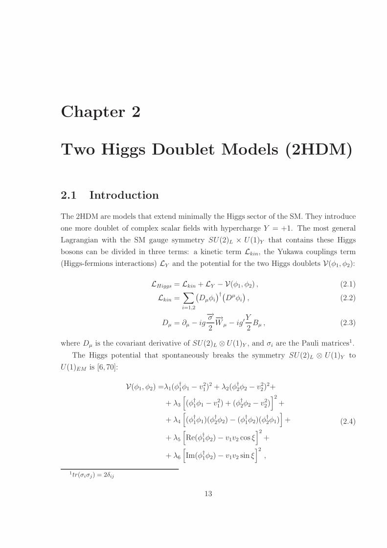
The 2HDM are models that extend minimally the Higgs sector of the SM. They introduce
one more doublet of complex scalar fields with hypercharge Y = +1. The most general
Lagrangian with the SM gauge symmetry SU(2)L × U(1)Y that contains these Higgs
bosons can be divided in three terms: a kinetic term Lkin, the Yukawa couplings term
(Higgs-fermions interactions) LY and the potential for the two Higgs doublets V(φ1, φ2):
LHiggs = Lkin + LY − V(φ1, φ2) , (2.1)
Lkin =∑
i=1,2
(
Dµφi)†(
Dµφi)
, (2.2)
Dµ = ∂µ − ig−→σ2
−→W µ − ig′
Y
2Bµ , (2.3)
where Dµ is the covariant derivative of SU(2)L ⊗ U(1)Y , and σi are the Pauli matrices1.
The Higgs potential that spontaneously breaks the symmetry SU(2)L ⊗ U(1)Y to
U(1)EM is [6, 70]:
V(φ1, φ2) =λ1(φ†1φ1 − v2
1)2 + λ2(φ
†2φ2 − v2
2)2+
+ λ3
[
(φ†1φ1 − v2
1) + (φ†2φ2 − v2
2)]2
+
+ λ4
[
(φ†1φ1)(φ
†2φ2)− (φ†
1φ2)(φ†2φ1)
]
+
+ λ5
[
Re(φ†1φ2)− v1v2 cos ξ
]2
+
+ λ6
[
Im(φ†1φ2)− v1v2 sin ξ
]2
,
(2.4)
1tr(σiσj) = 2δij
13

14 Two Higgs Doublet Models (2HDM)
where all the λi are real parameters, because the Lagrangian must be hermitic. This is the
most general Lagrangian compatible with the gauge symmetry and the discrete symmetry
φ1 → −φ1 [6, 70], this symmetry is only violated by soft terms of dimension two. We
impose this last symmetry to forbid the FCNC at tree level. Moreover, this potential
must be bounded from below, so the λi must be non-negative. But in fact, the allowed
range for the parameters λi corresponding to this minimum is a range in the parameter
space such that the square Higgs boson masses are positive and that V (0, 0) > 0.
In this context the minimum of the potential is:
〈φ1〉 ≡(
0
v1
)
, (2.5)
〈φ2〉 ≡(
0
v2eiξ
)
, (2.6)
which breaks the gauge symmetry giving U(1)EM .
We need two physical parameters in order to know their value, which are usually taken
to be:
M2W =
1
2g2(v2
1 + v22) ≡ g2v
2
2, tanβ =
v2
v1
, 0 < β <π
2. (2.7)
If we impose λ5 = λ6 (like in sypersymmetry) we can write the last two terms of
eq. (2.4) as:∣
∣
∣φ†
1φ2 − v1v2eiξ∣
∣
∣
2
. (2.8)
The phase ξ can disappear with a redefinition of the fields without affecting the others
terms of the potential (this phase will appear in other terms of the total Lagrangian).
Then, the Higgs potential is CP conserving.
At last, the final Higgs potential is:
V(φ1, φ2) =λ1(φ†1φ1 − v2
1)2 + λ2(φ
†2φ2 − v2
2)2+
+ λ3
[
(φ†1φ1 − v2
1) + (φ†2φ2 − v2
2)]2
+
+ λ4
[
(φ†1φ1)(φ
†2φ2)− (φ†
1φ2)(φ†2φ1)
]
+
+ λ5|φ†1φ2 − v1v2|2 .
(2.9)
There are different forms for the Yukawa terms of the Lagrangian to satisfy the
Glashow and Weinberg [71] theorem. The Glashow and Weinberg theorem says that
for a general SU(2)×U(1) gauge theory where we demand that the neutral-current inter-
actions conserve all quark flavor naturally the necessary and sufficient conditions are: All
quarks of fixed charge and helicity must (1) transform according to the same irreducible

2.1 Introduction 15
representations of weak SU(2), (2) correspond to the same eigenvalue of weak T3, and
(3) receive their contributions in the quark mass matrix form a single source (either from
the vacuum expectations value of a single neutral Higgs boson or from a unique gauge-
invariant bare mass term). In practice this implies that all fermions of a given electric
charge couple to no more than one Higgs doublet.
From the Lagrangian (2.4) with the potential (2.9) and the Yukawa terms we can
obtain the full 2HDM spectrum, as well as the interactions, which contain the usual SM
gauge interactions, the fermion-Higgs interactions, and the pure 2HDM interactions. A
detailed treatment of this Lagrangian, and the process of derivation of the forthcoming
results can be found in [72].
2.1.1 2HDM I
In this model one of the Higgs doublets (φ2) couple to all the fermions. The couplings
with the quarks is of the form:
L(I)Y = −
3∑
i,j=1
[
Dqij
(
q(i)L φ2
)
q(j)dR + U q
ij
(
q(i)L φ2
)
q(j)uR + h.c.
]
+ leptons , (2.10)
where
φ = iσ2φ∗ , (2.11)
q(i) =
(
q(i)u
q(i)d
)
, (2.12)
q(1) =
(
u
d
)
, q(2) =
(
c
s
)
, q(3) =
(
t
b
)
, (2.13)
and similarly for the leptonic doublets l(i) that contain the neutrinos and the leptons.
This model is very related with the minimal model (SM), being the only difference a
smaller VEV v2 < vSM (v ∼ 174GeV ) and bigger Yukawa couplings.
2.1.2 2HDM II
Now one doublet (φ1) couples to the right-handed (RH) down fermions (qdR, ldR) and is
responsible of the down masses; the other doublet (φ2) couples to the RH up fermions
(quR, luR) and is responsible of their masses. Taking any flavor base, i.e. one in which f(i)L
are isospin doublets the Lagrangian is:
L(II)Y = −
3∑
i,j=1
[
Dqij
(
q(i)L φ1
)
q(j)dR + U q
ij
(
q(i)L φ2
)
q(j)uR + h.c.
]
+ leptons . (2.14)

16 Two Higgs Doublet Models (2HDM)
The mass matrix will be proportional to the VEV of the Higgs as:
M (q,l)u = v2U
(q,l) , (2.15)
M(q,l)d = v1D
(q,l) , (2.16)
This is basically the Higgs sector required in the MSSM.
2.1.3 2HDM III
This is the most general 2HDM without FCNC at tree level, being the other two important
particular cases. The Yukawa interactions in this case, using any flavor base, is:
L(III)Y = −
3∑
i,j=1
[
Dq1,ij
(
q(i)L φ1
)
q(j)dR +Dq
2,ij
(
q(i)L φ2
)
q(j)dR+ (2.17)
+ U q1,ij
(
q(i)L φ1
)
q(j)uR + U q
2,ij
(
q(i)L φ2
)
q(j)uR + h.c.
]
+ (2.18)
+ [lHl terms] , (2.19)
where the 3× 3 matrices D1, D2, U1, U2 are such that diagonalize simultaneously with
the quark mass matrix.
2.2 2HDM spectrum
2.2.1 Higgs sector
We will use this structure for the doublets:
φi =
(
φ+i
Reφ0i + i Imφ0
i
)
i = 1, 2 . (2.20)
These fields are not physical fields, they do not have a well defined mass, as there are
bilinear terms within the scalar fields with different fields. The next thing is to diagonalize
the mass matrix. It can be seen that the mass matrix is a diagonal matrix in boxes for the
fields a) φ+1 , φ
+2 , b) Reφ0
1,Reφ02 and c) Imφ0
1, Imφ02 (the real and imaginary part can be
treated separately by CP invariance). So we have to separately diagonalize the different
boxes. If we define the rotation angle as:
R(ω) =
(
cosω sinω
− sinω cosω
)
, (2.21)
the rotations (transformations) of the fields are:

2.2 2HDM spectrum 17
(
G±
H±
)
= R(β)
(
φ±1
φ±2
)
, (2.22)
(
H0
h0
)
=√
2R(α)
(
Reφ01 − v1
Reφ02 − v2
)
, (2.23)
(
G0
A0
)
=√
2R(β)
(
Imφ01
Imφ02
)
, (2.24)
with their masses:
m2H± = λ4(v
21 + v2
2) , (2.25)
m2A0 = λ5(v
21 + v2
2) , (2.26)
m2H0,h0 =
1
2
[
M11 +M22 ±√
(M11 −M22)2 + 4M212
]
, (2.27)
where Mij are defined from the CP-even mass matrix
M =
(
4v21(λ1 + λ3) + v2
2λ5 (4λ3 + λ5)v1v2
(4λ3 + λ5)v1v2 4v22(λ2 + λ3) + v2
1λ5
)
. (2.28)
The mixing angles β and α are:
tan β =v2
v1
, (2.29)
sin 2α =2M12
√
(M11 −M22)2 + 4M212
,
cos 2α =M11 −M22
√
(M11 −M22)2 + 4M212
. (2.30)
Now we can redefine the parameters of the theory as:
4 masses : mh0 , mH0 , mA0, mH± (2.31)
2 mixing angles : α, β (2.32)
At tree level we get:
GF√2
=g2
8M2W
, (2.33)
where we find the value of v
v =√
v21 + v2
2 = 2−3/4G−1/2F ∼ 174GeV. (2.34)
18 Two Higgs Doublet Models (2HDM)
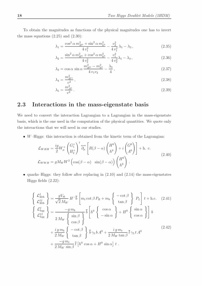
To obtain the magnitudes as functions of the physical magnitudes one has to invert
the mass equations (2.25) and (2.30):
λ1 =cos2 αm2
H0 + sin2 αm2h0
4 v21
− v22
4 v21
λ5 − λ3 , (2.35)
λ2 =sin2 αm2
H0 + cos2 αm2h0
4 v22
− v21
4 v22
λ5 − λ3 , (2.36)
λ3 = cosα sinαm2H0 −m2
h0
4 v1v2
− λ5
4, (2.37)
λ4 =m2H±
v2, (2.38)
λ5 =m2A0
v2. (2.39)
2.3 Interactions in the mass-eigenstate basis
We need to convert the interaction Lagrangian to a Lagrangian in the mass-eigenstate
basis, which is the one used in the computation of the physical quantities. We quote only
the interactions that we will need in our studies.
• W–Higgs: this interaction is obtained from the kinetic term of the Lagrangian:
LWHH =ig
2W+µ
(
G+1
H+2
)†←→∂µ
[
R(β − α)
(
H0
h0
)
+ i
(
G0
A0
)]
+ h. c.
LWWH = gMWW2(
cos(β − α) sin(β − α))
(
H0
h0
)
.
(2.40)
• quarks–Higgs: they follow after replacing in (2.10) and (2.14) the mass-eigenstates
Higgs fields (2.22):
{
LIHtbLIIHtb
}
=gVtb√2MW
H−b
[
mt cot β PR +mb
{
− cot β
tan β
}
PL
]
t+ h.c. (2.41)
{
LIhqqLIIhqq
}
=−g mb
2MW
{
sin β
cosβ
} b
[
h0
{
cosα
− sinα
}
+H0
{
sinα
cosα
}]
b
+i g mb
2MW
{
− cot β
tanβ
}
b γ5 bA0 +
i g mt
2MW tanβt γ5 t A
0
+−g mt
2MW sin βt[
h0 cosα+H0 sinα]
t .
(2.42)
2.3 Interactions in the mass-eigenstate basis 19
H±H∓H0 − gMW sin 2β
[
(m2H± −m2
A0 + 12m2H0) sin 2β cos(β − α)+
+(m2A0 −m2
H0) cos 2β sin(β − α)]
H±H∓h0 − gMW sin 2β
[
(m2H± −m2
A0 + 12m2h0) sin 2β sin(β − α)+
+(m2h0 −m2
A0) cos 2β cos(β − α)]
h0h0H0 − g cos(β−α)2MW sin 2β
[
(2m2h0 +m2
H0) sin 2α−−m2
A0 (3 sin 2α− sin 2β)]
A0A0H0 − g2MW sin 2β
[
m2H0 sin 2β cos(β − α)+
+2(m2H0 −m2
A0) cos 2β sin(β − α)]
A0A0h0 − g2MW sin 2β
[
m2h0 sin 2β sin(β − α)+
+2(m2h0 −m2
A0) cos 2β cos(β − α)]
H± −H∓ −A0 0
H± −G∓ −H0 (−ig)(m2H± −m2
H0)sin(β − α)
2MW
H± −G∓ − h0 ig(m2H± −m2
h0)cos(β − α)
2MW
H± −G∓ − A0 ±g (m2H± −m2
A0)
2MW
G± −G∓ −H0 (−ig)m2H0 cos(β − α)
2MW
G± −G∓ − h0 (−ig)m2h0 sin(β − α)
2MW
G± −G∓ − A0 0
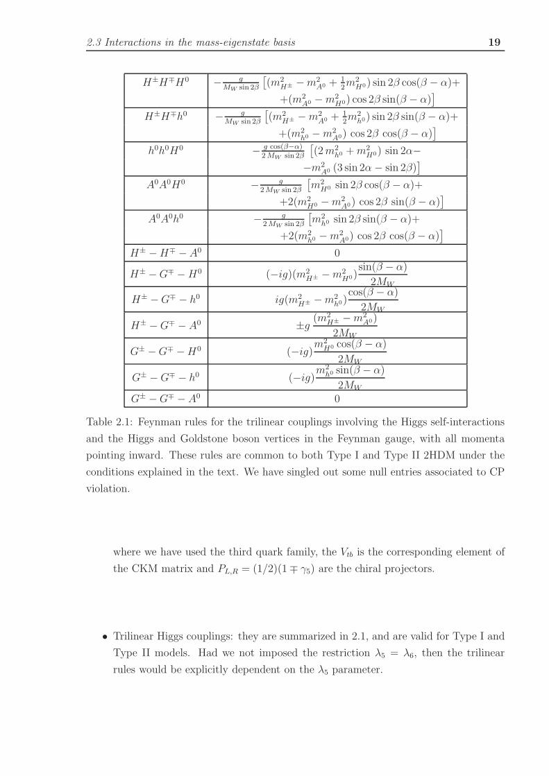
Table 2.1: Feynman rules for the trilinear couplings involving the Higgs self-interactions
and the Higgs and Goldstone boson vertices in the Feynman gauge, with all momenta
pointing inward. These rules are common to both Type I and Type II 2HDM under the
conditions explained in the text. We have singled out some null entries associated to CP
violation.
where we have used the third quark family, the Vtb is the corresponding element of
the CKM matrix and PL,R = (1/2)(1∓ γ5) are the chiral projectors.
• Trilinear Higgs couplings: they are summarized in 2.1, and are valid for Type I and
Type II models. Had we not imposed the restriction λ5 = λ6, then the trilinear
rules would be explicitly dependent on the λ5 parameter.

20 Two Higgs Doublet Models (2HDM)
2.4 Constraints
There are multiple constraints that must be imposed, obviously one of such constraints
is that they must reproduce the behaviour of the SM up to energy scales probed so far.
Analysing the perturbativity of the theory one finds that the allowed range for tan β
is:
0.1 < tan β . 60 . (2.43)
The custodial symmetry [73, 74] (SU(2)) is a good symmetry at tree level, so the
quadratic violations of this symmetry must be experimentally fixed. So, the one-loop
corrections of the parameter ρ from the 2HDM sector can not be bigger than one per mil
of the SM [75]:
|δρ2HDM| 6 0.001 . (2.44)
To be precise, the latter is the extra effect that δρ can accommodate at one standard
deviation (1 σ) from the 2HDM fields beyond the SM contribution [43]. This is a stringent
restriction that affects the possible mass splittings among the Higgs fields of the 2HDM,
and its implementation in our codes does severely prevent the possibility from playing
with the Higgs boson masses to artificially enhance the FCNC contributions.
Moreover, the charged Higgs bosons have an important indirect restriction from the
radiative decays of the B meson, specially the ratio B(B → Xs γ) – or B(b→ sγ) at the
quark level [52–58]:
B(b→ sγ) = (3.3± 0.4)× 10−4 . (2.45)
The Higgs contribution to B(b→ sγ) (that have been computed at the NLO in QCD [62])
is positive: bigger experimental ratio means that the charged Higgs mass can be smaller.
From the different analysis of the literature [59–62] we get:
mH± > 350GeV (2.46)
for virtually any tanβ & 1. This bound does not apply to Type I models because at
large tanβ the charged Higgs couplings are severely suppressed, whereas at low tan β we
recover the previous unrestricted situation of Type II models.
We can derive lower bounds for the neutral Higgs masses in these models [76, 77].
For example, using the Bjorken process e+e− → Z + h0 and the production of pairs of
Higgs boson e+e− → h0(H0) + A0 we can get the following restrictions in almost all the
parameter space [78, 79]:
mh0 +mA0
& 100GeV ∀ tan β
& 150GeV tan β > 1. (2.47)
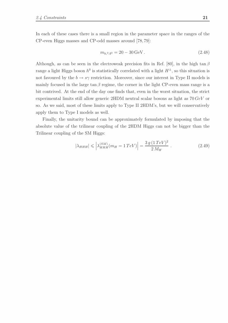
2.4 Constraints 21
In each of these cases there is a small region in the parameter space in the ranges of the
CP-even Higgs masses and CP-odd masses around [78, 79]:
mh,0A0 = 20− 30GeV . (2.48)
Although, as can be seen in the electroweak precision fits in Ref. [80], in the high tanβ
range a light Higgs boson h0 is statistically correlated with a light H±, so this situation is
not favoured by the b→ sγ restriction. Moreover, since our interest in Type II models is
mainly focused in the large tan β regime, the corner in the light CP-even mass range is a
bit contrived. At the end of the day one finds that, even in the worst situation, the strict
experimental limits still allow generic 2HDM neutral scalar bosons as light as 70GeV or
so. As we said, most of these limits apply to Type II 2HDM’s, but we will conservatively
apply them to Type I models as well.
Finally, the unitarity bound can be approximately formulated by imposing that the
absolute value of the trilinear coupling of the 2HDM Higgs can not be bigger than the
Trilinear coupling of the SM Higgs:
|λHHH | 6∣
∣
∣λ
(SM)HHH(mH = 1TeV )
∣
∣
∣=
3 g (1 TeV )2
2MW. (2.49)
Chapter 3
The Minimal Supersymmetric
Standard Model (MSSM)
3.1 Introduction
It goes beyond the scope of this Thesis to study the formal theory of Supersymmetry
[81, 82], however we would like, at least, to give a feeling on what is it. Supersymmetry
(SUSY) can be introduced in many manners.
Let us consider the symmetries of the scattering matrix S, that is, those transforma-
tions that can be reduced to an interchange of asymptotic states. Before the discovery of
Supersymmetry the only symmetries know were: the following: (1) the ones correspond-
ing to the Poincare group; (2) the so called internal global symmetries, both of them ruled
by a Lie algebra; and (3) discrete symmetries such as parity (P), charge conjugations (C)
and the time reversal (T). A 1967 theorem due to Coleman and Mandula establishes rig-
orously that, under very general conditions, these are the only symmetries allowed for S if
we do not want to induce trivial scattering (fixed angles and speeds) in 2→ 2 processes.
This theorem may be eluded relaxing some of its hypotheses. The Supersymmetry
appears precisely when assuming that the generators of the new symmetry we want to
add have a spinorial character instead of a scalar one, therefore transforming under (12, 0)
and (0, 12) representations of the Lorentz group. Fermionic spinorial generators necessarily
have an anti-commutative algebra, generically known as a graded Lie algebra. The algebra
is not closed with just the SUSY generators, thus it can not be understood as an internal
symmetry, but it rather forms an extension of the space-time symmetries of the Poincare
group.
Following this line of thought, one could relax some other hypotheses of the Coleman-
23

24 The Minimal Supersymmetric Standard Model (MSSM)
Mandula theorem in order to introduce new theories. SUSY is the only known extension
for the S matrix symmetries. Accepting as the only valid extensions of the Coleman-
Mandula theorem conditions the presence of a graded Lie algebra, one can show (Haag,
Lopuszanki and Sohnius theorem) that spinorial generators different from those of SUSY
are forbidden.
Next, we have to define the “superspace”, the supersymmetric space of the “super-
fields”. We add to the space-time coordinates x other sets of spinorial coordinates (θ, θ)
(as many sets as the dimension of the space-time) that are Grassmann variables, i.e.
they anti-commute. In the case of adding just one set it is said that we have a N = 1
Supersymmetry and a N = 1 superspace:
space − time → N = 1 Superspace
xµ → (xµ, θα, θα) (3.1)
where α = 1, 2. The supersymmetric transformations have the parameters (Λ, a, ξ, ξ),
where Λ is the Lorentz matrix, a is the translation 4-vector, and the Weyl spinors ξ, ξ.
The generators of SUSY transformations consist of are the ones of the Poincare group
and the new spinorial generators Qα and Qα, satisfying the graded Lie algebra. The
infinitesimal purely SUSY transformation of a superfield Φ(x, θ, θ) is:
Φ→ Φ + δSΦ (3.2)
δS = −i(ξαQα + ξαQα) (3.3)
The functions defined in the Superspace are polynomial functions of the (θ, θ) variables
(since θ2α = θ2
α = 0). Thus we can decompose the functions (superfields) of this Superspace
in components of θ0, θα, θα, θαθβ, . . . each of these components will be a function of the
space-time coordinates. Analogously to the space-time, we can define in the Superspace
scalar superfields, vector superfields, . . . For example in a 4-dimensional space time with
N = 1 supersymmetry a scalar superfield has 10 components.
We can define fields with specific properties with respect to the θ variables [81,82]. A
scalar chiral field in a 4D N = 1 Superspace has 4 components:
ΦL = A +√
2θψ + θθF ≡ (A,ψ, F ) (3.4)
ΦR = A∗ +√
2θψ + θθF ∗ ≡ (A∗, ψ, F ∗) (3.5)
where A is a scalar field, ψ and ψ are Weyl spinors (left-handed and right handed
Dirac fermions) and F is an auxiliary scalar field. This auxiliary field is not a dynamical
field since its equations of motion do not involve time derivatives. To this end we are left

3.1 Introduction 25
with a superfield, whose components represent an ordinary scalar field and an ordinary
chiral spinor. So if nature is described by the dynamics of this field we would find a chiral
fermion and a scalar with identical quantum numbers. That is Supersymmetry relates
particles which differ by spin 1/2. When a SUSY transformation (Q) acts on a superfield
it transform spin s particles into spin s± 1/2 particles.
Thus, for a N = 1 SUSY, we find that to any chiral fermion there should be a scalar
particle with exactly the same properties. This fact is on the basis of the absence of
quadratic divergences in boson mass renormalization, since for any loop diagram involving
a scalar particle there should be a fermionic loop diagram, which will cancel quadratic
divergences between each other, though logarithmic divergences remain.
Supersymmetric interactions can be introduced by means of generalized gauge trans-
formations, and by means of a generalized potential function, the Superpotential, which
give rise to masses, Yukawa-type interactions, and a scalar potential.
As no scalar particles have been found at the electroweak scale we may infer that, if
SUSY exists, it is broken. We can allow SUSY to be broken maintaining the property that
no quadratic divergences are allowed: this is the so called Soft-SUSY-Breaking mechanism
[83]. We can achieve this by only introducing a small set of SUSY-Breaking terms in the
Lagrangian, to wit: masses for the components of lowest spin of a supermultiplet and triple
scalar interactions. However, other terms like explicit fermion masses for the matter fields
would violate the Soft-SUSY-Breaking condition.
The MSSM is the minimal Supersymmetric extension of the Standard Model. It is
introduced by means of a N = 1 SUSY, with the minimum number of new particles. Thus
for each fermion f of the SM there are two scalars related to its chiral components called
“sfermions” (fL,R), for each gauge vector V there is also a chiral fermion: “gaugino” (v),
and for each Higgs scalar H another chiral fermion: “higgsino” (h). In the MSSM it turns
out that, in order to be able of giving masses to up-type and down-type fermions, we
must introduce two Higgs doublets with opposite hypercharge, and so the MSSM Higgs
sector is of the so called Type II 2HDM (see chapter 2, section 3.4.1 and Ref. [6]).
To build the MSSM Lagrangian we must build a Lagrangian invariant under the
gauge group SU(3)C × SU(2)L × U(1)Y , it must also include the superfields with the
particle content of the Table 3.1 and in addition it must contain the terms that breake
supersymmetry softly. But this Lagrangian violates the baryonic and leptonic number, so
we have to introduce an additional symmetry. In the case of the MSSM this symmetry
is the so-called R-symmetry. In its discrete form it relates the spin (S), the baryonic
number (B) and the leptonic number (L) in the so-called R-parity:
R = (−1)2S+L+3B (3.6)

26 The Minimal Supersymmetric Standard Model (MSSM)
so that is 1 for the SM fields and−1 for its supersymmetric partners. In the way the MSSM
is implemented R-parity is conserved, this means that R-odd particles (the superpartners
of SM particles) can only be created in pairs, also that in the final product decay of an
R-odd particle at least one SUSY particle exists, and that the Lightest Supersymmetric
Particle (LSP) is stable.
3.2 Field content
The field content of the MSSM consist of the fields of the SM plus all their supersymmetric
partners, and an additional Higgs doublet. The Table 3.1 shows all the correspondences
and all the fields. All these fields suffer some mixing, so the physical (mass eigenstates)
fields look much different from these ones, as shown in Table 3.2. The gauge fields mix up
to give the well known gauge bosons of the SM, W±µ , Z0
µ, Aµ, the gauginos and higgsinos
mix up to give the chargino and neutralino fields, and finally the Left- and Right-chiral
sfermions mix among themselves in sfermions of indefinite chirality. Letting aside the
intergenerational mixing between fermions and sfermions that give rise to the well known
Cabibbo-Kobayashi-Maskawa (CKM and superCKM) matrix.
Superfield SM particle Sparticle SU(3)C SU(2)L U(1)Y
Matter
L
Rleptons
L = (νl, l)L
R = l−L
sleptons
L = (νlL, lL)
R = l+R
1
1
2
1
−1
2
Q
U
D
quarks
Q = (u, d)L
U = ucL
D = dcL
squarks
Q = (uL, dL)
U = u∗R
D = d∗R
3
3∗
3∗
2
1
1
1/3
−4/3
2/3
H1
H2
Higgs
H1 = (H01 , H
−1 )
H2 = (H+2 , H
02 )
Higgsinos
H1 = (H01 , H
−1 )
H2 = (H+2 , H
02 )
1
1
2
2
−1
1
Gauge
G gluon gµ gluino g 8 0 0
V w (W1,W2,W3) wino (W1, W2, W3) 1 3 0
V ′ b B0 bino (B0 1 1 0
Table 3.1: Particle contents of the MSSM superfields
3.3 Lagrangian 27
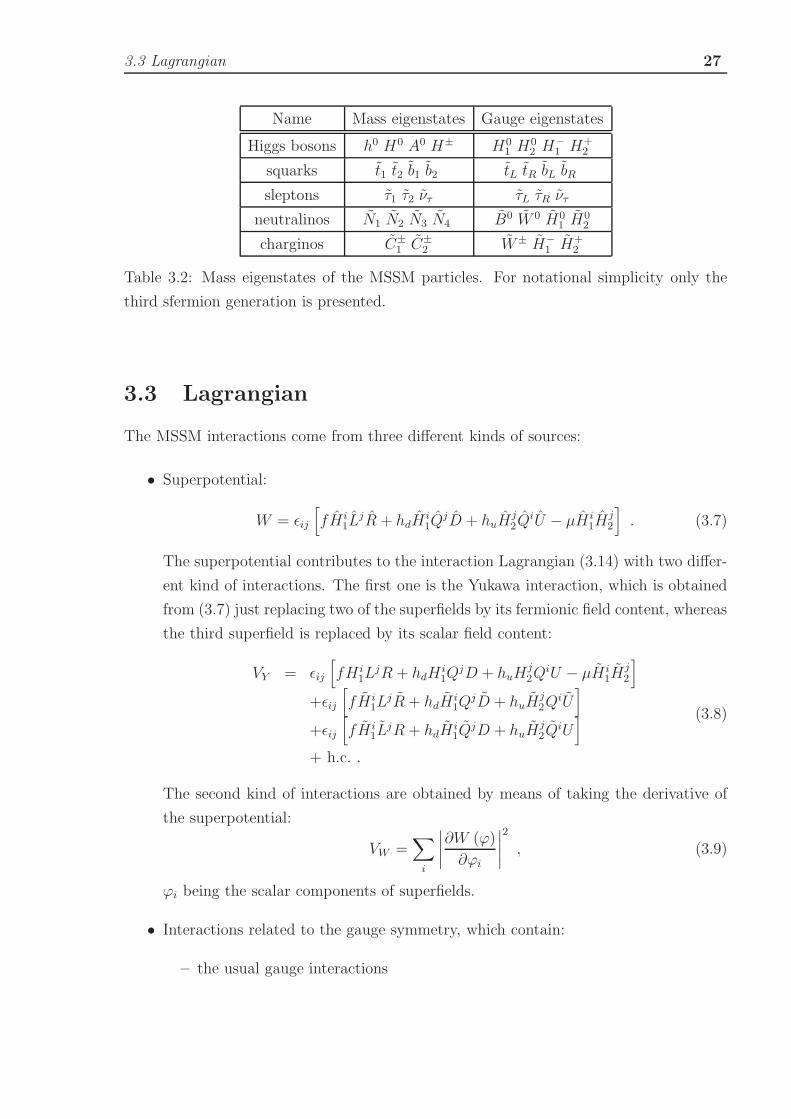
Name Mass eigenstates Gauge eigenstates
Higgs bosons h0 H0 A0 H± H01 H
02 H
−1 H+
2
squarks t1 t2 b1 b2 tL tR bL bR
sleptons τ1 τ2 ντ τL τR ντ
neutralinos N1 N2 N3 N4 B0 W 0 H01 H
02
charginos C±1 C±
2 W± H−1 H+
2
Table 3.2: Mass eigenstates of the MSSM particles. For notational simplicity only the
third sfermion generation is presented.
3.3 Lagrangian
The MSSM interactions come from three different kinds of sources:
• Superpotential:
W = ǫij
[
fH i1L
jR+ hdHi1Q
jD + huHj2Q
iU − µH i1H
j2
]
. (3.7)
The superpotential contributes to the interaction Lagrangian (3.14) with two differ-
ent kind of interactions. The first one is the Yukawa interaction, which is obtained
from (3.7) just replacing two of the superfields by its fermionic field content, whereas
the third superfield is replaced by its scalar field content:
VY = ǫij
[
fH i1L
jR+ hdHi1Q
jD + huHj2Q
iU − µH i1H
j2
]
+ǫij
[
fH i1L
jR+ hdHi1Q
jD + huHj2Q
iU]
+ǫij
[
fH i1L
jR+ hdHi1Q
jD + huHj2Q
iU]
+ h.c. .
(3.8)
The second kind of interactions are obtained by means of taking the derivative of
the superpotential:
VW =∑
i
∣
∣
∣
∣
∂W (ϕ)
∂ϕi
∣
∣
∣
∣
2
, (3.9)
ϕi being the scalar components of superfields.
• Interactions related to the gauge symmetry, which contain:
– the usual gauge interactions

28 The Minimal Supersymmetric Standard Model (MSSM)
– the gaugino interactions:
VGψψ = i√
2gaϕkλa (T a)kl ψl + h.c. (3.10)
where (ϕ, ψ) are the spin 0 and spin 1/2 components of a chiral superfield
respectively, T a is a generator of the gauge symmetry, λa is the gaugino field
and ga its coupling constant.
– and the D-terms, related to the gauge structure of the theory, but that do not
contain neither gauge bosons nor gauginos:
VD =1
2
∑
DaDa , (3.11)
with
Da = gaϕ∗i (T a)ij ϕj , (3.12)
ϕi being the scalar components of the superfields.
• Soft-SUSY-Breaking interaction terms:
V Isoft =
g√2MW cosβ
ǫij
[
mlAlHi1L
jR+mdAdHi1Q
jD −muAuHi2QU
]
+ h.c. .
(3.13)
The trilinear Soft-SUSY-Breaking couplings Af can play an important role, specially
for the third generation interactions and masses, and they are in the source of the
large value of the bottom quark mass renormalization effects.
The full MSSM Lagrangian is then:
LMSSM = LKinetic + LGauge − VGψψ − VD − VY −∑
i
∣
∣
∣
∣
∂W (ϕ)
∂ϕi
∣
∣
∣
∣
2
−V Isoft −m2
1H†1H1 −m2
2 H†2H2 −m2
12
(
H1H2 +H†1H
†2
)
−1
2mg ψ
agψ
ag −
1
2M wiwi −
1
2M ′ B0B0
−m2LL∗L−m2
RR∗R −m2
QQ∗Q−m2
UU∗U −m2
DD∗D , (3.14)
where we have also included the Soft-SUSY-breaking masses.
From the Lagrangian (3.14) we can obtain the full MSSM spectrum, as well as the
interactions, which contain the usual SM gauge interactions, the fermion-Higgs interac-
tions that correspond to a Type II Two-Higgs-Doublet Model [6], and the pure SUSY
interactions. A very detailed treatment of this Lagrangian, and the process of derivation
of the forthcoming results can be found in [84].
3.4 MSSM spectrum 29
3.4 MSSM spectrum
3.4.1 Higgs boson sector
As seen in 2.1, when a Higgs doublet is added to the SM there exist two possibilities for
incorporating it, avoiding Flavour Changing Neutral Currents (FCNC) at tree level [6].
The first possibility is not to allow a coupling between the second doublet and the fermion
fields, this is the so called Type I 2HDM. The second possibility is to allow both Higgs
doublets to couple with fermions, the first doublet only coupling to the Right-handed
down-type fermions, and the second one to Right-handed up-type fermions, this is the so
called Type II 2HDM.
The Higgs sector of the MSSM is that of a Type II 2HDM [6], with some SUSY
restrictions. After expanding (3.14) the Higgs potential reads
V = m21 |H1|2 +m2
2 |H2|2 −m212
(
ǫij Hi1H
j2 + h.c.
)
+1
8(g2 + g′2)
(
|H1|2 − |H2|2)2
+1
2g2 |H†
1 H2|2 . (3.15)
This is equivalent to the 2HDM potential (2.9) with the following restrictions:
λ1 = λ2 (3.16)
λ3 =1
8(g2 + g′2)− λ1 (3.17)
λ4 = 2λ1 −1
2g2 (3.18)
λ5 = λ6 = 2λ1 −1
2(g2 + g′2). (3.19)
The neutral Higgs bosons fields acquire a vacuum expectation value (VEV),
〈H1〉0 =
(
v1
0
)
〈H2〉0 =
(
0
v2
)
. (3.20)
We need two physical parameters in order to know their value, which are usually taken
to be MW and tan β:
M2W =
1
2g2(v2
1 + v22) ≡ g2v
2
2(3.21)
M2Z =
1
2(g2 + g′2)v2 ≡M2
W cos2 θW (3.22)
tanβ =v2
v1
, 0 < β <π
2(3.23)
tan θW =g′
g(3.24)
30 The Minimal Supersymmetric Standard Model (MSSM)
These VEV’s make the Higgs fields to mix up. There are five physical Higgs fields: a
couple of charged Higgs bosons (H±); a “pseudoscalar” Higgs (CP = −1) A0; and two
scalar Higgs bosons (CP = 1) H0 (the heaviest) and h0 (the lightest). There are also the
Goldstone bosons G0 and G±. The relation between the physical Higgs fields and that
fields of (3.2) is
(
−H±1
H±2
)
=
(
cosβ − sin β
sin β cos β
)(
G±
H±
)
, (3.25)
(
H01
H02
)
=
(
v1
v2
)
+1√2
(
cosβ − sin β
sin β cosβ
)(
H0
h0
)
(3.26)
+i√2
(
−(cos β − sin β)
sin β cosβ
)(
G0
A0
)
where α is given in (3.28) [6].
All the masses of the Higgs sector of the MSSM can be obtained with only two pa-
rameters, the first one is tan β (3.24), and the second one is a mass; usually this second
parameter is taken to be either the charged Higgs mass mH± or the pseudoscalar Higgs
mass mA0 . We will take the last option. From (3.15) one can obtain the tree-level mass
relations between the different Higgs particles,
m2H± = m2
A0 +M2W ,
m2H0,h0 =
1
2
(
m2A0 +M2
Z ±√
(
m2A0 +M2
Z
)2 − 4m2A0 M2
Z cos2 2β
)
, (3.27)
and the mixing angle between the two scalar Higgs is obtained by means of:
cos 2α = − cos 2β
(
m2A0 −M2
Z
m2H0 −m2
h0
)
, sin 2α = − sin 2β
(
m2H0 +m2
h0
m2H0 −m2
h0
)
. (3.28)
The immediate consequence of such a constrained Higgs sector, is the existence of absolute
bounds (at tree level) for the Higgs masses:
0 < mh0 < MZ < mH0 , MW < mH± . (3.29)
It must be taken into account, though, that the radiative corrections, mainly due to the
top-stop supermultiplet, and also the bottom-sbottom one, are susceptible of relaxing the
limits (3.29) in a significant manner.
A good approximation for effective mixing angle αeff including only the leading one-
loop contributions of top, stop, bottom and sbottom follows from the diagonalization of

3.4 MSSM spectrum 31
the one-loop Higgs mass matrix [85–88]:
M2Higgs =
sin 2β
2
(
cotβ M2Z + tanβ m2
A0 + σt + ωb −M2Z −m2
A0 + λt + λb
−M2Z −m2
A0 + λt + λb tanβ M2Z + cotβ m2
A0 + ωt + λb
)
.
(3.30)
where
ωt =NCGFm
4t√
2π2 sin2 β
(
log (mt1mt2
m2t
) +At(At − µ cotβ)
m2t1−m2
t2
logm2t1
m2t2
+A2t (At − µ cotβ)2
(m2t1−m2
t2)2
(
1−m2t1
+m2t2
m2t1−m2
t2
logmt1
mt2
) )
λt = − NCGFm4t√
2π2 sin2 β
(
µ(At − µ cotβ)
m2t1−m2
t2
logm2t1
m2t2
+2µAt(At − µ cotβ)2
(m2t1−m2
t2)2
(
1−m2t1
+m2t2
m2t1−m2
t2
logmt1
mt2
) )
σt =NCGFm
4t√
2π2 sin2 β
µ2(At − µ cotβ)2
(m2t1−m2
t2)2
(
1−m2t1
+m2t2
m2t1−m2
t2
logmt1
mt2
)
(3.31)
with the following substitutions for the bottom/sbottom factors:
(ωb, λb, σb)↔ (ωt, λt, σt) with
t ↔ b
sin β ↔ cosβ
At − µ cotβ ↔ Ab − µ tanβ
(3.32)
This approximate effective mixing angle αeff is determined by
tanαeff =−(m2
A0 +M2Z) tanβ + (λt + λb)(1 + tan2β)/2
M2Z +m2
A0 tan2 β + (σt + ωb −M2h0,eff)(1 + tan2β)
, (3.33)
where Mh0,eff is the solution for the light Higgs mass:
M2H0,h0, eff =
m2A0 +M2
Z + ωt + σt + ωb + σb2
±(
(m2A0 +M2
Z)2 + (ωt − σt + σb − ωb)2
4
−m2A0M2
Z cos2 2β +(ωt − σt + σb − ωb) cos 2β
2(m2
A0 −M2Z)
−(λt + λb sin 2β)
2(m2
A0 +M2Z) +
(λt + λb)2
4
)1/2
. (3.34)
In the limit where mA0 ≫ MZ , cos(β − α) = O(M2Z/m
2A0), which means that the
h0 couplings to Standard Model particles approach values corresponding precisely to the
couplings of the SM Higgs boson. There is a significant region of MSSM Higgs sector

32 The Minimal Supersymmetric Standard Model (MSSM)
50 100 500 1000m
A0 [GeV]
1e-07
1e-06
1e-05
0.0001
0.001
0.01
0.1
1
cos2 (β
−α)
tanβ = 5 tanβ = 50
MSUSY
= 1 TeV
µ = - 1 TeV
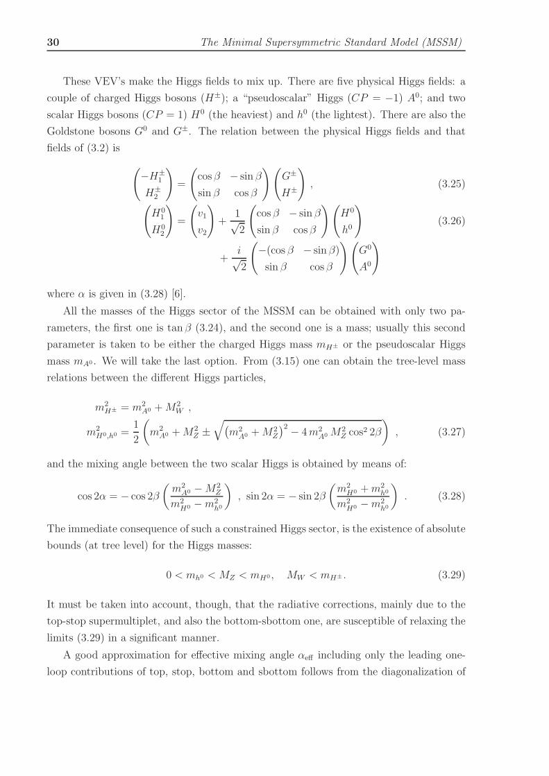
Figure 3.1: The value of cos2(β − α) is shown as a function of mA0 for two choices of
tanβ = 5 and tan β = 50. When radiative-corrections are included, one can define an
approximate loop-corrected angle α as a function ofmA0 , tan β and the MSSM parameters.
In the figures above, we have incorporated radiative corrections, assuming that MSUSY ≡mq = md = mu = 1TeV. The decoupling effect, in which cos2(β − α) ∝ M4
Z/mA04 for
mA0 ≫ mZ , continues to hold even when radiative corrections are included.
parameter space in which the decoupling limit applies, because cos(β−α) approaches zero
quite rapidly once mA0 is larger than about 200 GeV, as shown in Fig. 3.1. As a result,
over a significant region of the MSSM parameter space, the search for the lightest CP-even
Higgs boson of the MSSM is equivalent to the search for the SM Higgs boson. This result
is more general; in many theories of non-minimal Higgs sectors, there is a significant
portion of the parameter space that approximates the decoupling limit. Consequently,
simulations of the SM Higgs signal are also relevant for exploring the more general Higgs
sector.
3.4.2 The SM sector
In this section we give some expressions to obtain some MSSM parameters as a function
of the SM parametrization.
As stated above (sec. 3.4.1) the VEV’s can be obtained by means of (3.24), and the

3.4 MSSM spectrum 33
Z mass can be obtained at tree-level by the relation:
sin2 θW = 1− M2W
M2Z
.
Fermion masses are obtained from the Yukawa potential (3.8) letting the neutral Higgs
fields acquire their VEV (3.20). The up-type fermions get their masses from the H02
whereas H01 gives masses to down-type fermions, so
mu = huv2 =hu√
2MW sin β
g, md = hdv1 =
hd√
2MW cosβ
g,
and the Yukawa coupling can be obtained as
λu =hug
=mu√
2MW sin β, λd =
hdg
=md√
2MW cosβ. (3.35)
3.4.3 Sfermion sector (Flavor-diagonal case)
The sfermion mass terms are obtained from the derivative of the superpotential (3.9), the
D-terms (3.11) and the Soft-SUSY-Breaking terms (3.14) letting the neutral Higgs fields
get their VEV (3.20), and one obtain the following mass matrices:
M2q =
(
M2qL
+m2q + cos 2β(T qL3 −Qqs
2W )M2
Z mqMqLR
mqMqLR M2
qR+m2
q + cos 2β Qq s2W M2
Z
)
, (3.36)
being Q the corresponding fermion electric charge, T qL3 the third component of weak
isospin, MqL,Rthe Soft-SUSY-Breaking squark masses [7–10] (by SU(2)L-gauge invariance,
we must have MtL = MbL, whereas MtR , MbR
are in general independent parameters),
sθ = sin θW , and
MuLR = Au − µ cotβ ,
MdLR = Ad − µ tanβ . (3.37)
We define the sfermion mixing matrix as (q′a = {q′1 ≡ qL, q′2 ≡ qR} are the weak-
eigenstate squarks, and qa = {q1, q2} are the mass-eigenstate squark fields)
q′a =∑
b
R(q)ab qb,
R(q) =
(
cos θq − sin θq
sin θq cos θq
)
. (3.38)
R(q)†M2qR
(q) = diag{m2q2, m2
q1} (mq2 ≥ mq1) , (3.39)

34 The Minimal Supersymmetric Standard Model (MSSM)
tan 2θq =2mqM
qLR
M2qL−M2
qR+ cos 2β(T qL3 − 2Qqs
2W )M2
Z
. (3.40)
From eq. (3.36) we can see that the sfermion mass is dominated by the Soft-SUSY-
Breaking parameters (Mf ≫ mf for f 6= top), and that the non-diagonal terms could
be neglected, except in the case of the top squark (and bottom squark at large tanβ),
however we will maintain those terms, the reason is that, although the A parameters do
not play any role when computing the sfermion masses, they do play a role in the Higgs-
sfermion-sfermion coupling, and thus it has an effect on the Higgs self-energies. Moreover
these A parameters are constrained by the approximate (necessary) condition of absence
of colour-breaking minima,
A2q < 3 (m2
t +m2b+M2
H + µ2) , (3.41)
where mq is of the order of the average squark masses for q = t, b [89–92].
All the Soft-SUSY-Breaking parameters are free in the strict MSSM, however some
simplifications must be done to be able of making a feasible numerical analysis. As the
main subject of study are the third generation squarks we make a separation between
them and the rest of sfermions. This separation is justified by the evolution of the squark
masses from the (supposed) unification scale down to the electroweak scale [12] (see also
section 3.7.1 for a more detailed discussion).
So we will use the following approximations:
• equality of the diagonal elements of eq. (3.36)
M2qD ≡M2
q11 =M2q22 , (3.42)
for each charged slepton and each squark of the the first and second generation.
• the first and second generation squarks share the same value of the A parame-
ter (3.37) and the mass parameter (3.42)
• sleptons also share the same value for (3.42) and A parameters (3.37).
3.4.4 Sfermion sector (Non-flavor-diagonal case)
Very important for our FCNC studies is when the squark mass matrix does not diagonalize
with the same matrix as the one for the quarks. We introduce then intergenerational mass
terms for the squarks, but in order to prevent the number of parameters from being too
large, we have allowed (symmetric) mixing mass terms only for the left-handed squarks.
This simplification is often used in the MSSM, and is justified by RGE analysis [93].

3.5 Interactions in the mass-eigenstate basis 35
The flavor mixing terms are introduced through the parameters δij defined as
(M2LL)ij = m2
ij ≡ δijmimj , (3.43)
where mi is the mass of the left-handed i squark, and m2ij is the mixing mass matrix
element between the generations i and j. Thus we must diagonalize two 6 × 6 mass
matrices in order to obtain the mass-eigenstates squark fields. Generalizing the notation
in Sec. 3.4.3 we introduce the 6× 6 mixing matrices as follows:
q′α =∑
β
R(q)αβ qβ (3.44)
R(q)†M2qR = M2
qD = diag{m2q1 , . . . , m
2q6} , q ≡ u, d , (3.45)
where M2(u,d)
is the 6 × 6 square mass matrix for up-type (or down-type) squarks in
the EW basis, with indices α = 1, 2, 3, . . . , 6 ≡ uL, uR, . . . , tR for up-type squarks, and
similarly for down-type squarks. In this study we are only interested in the up-type quarks-
squarks system, so we will drop out the (q) super-index in the forthcoming expressions.
The rotation matrix R introduces gluino mediated tree-level FCNC between quarks and
squarks.
To analyze the contributions from these flavor and chiral mixed squarks we can use the
so-called mass insertion approximation. This is based on the fact that the δij parameters
are small, so instead of diagonalizing the 6 × 6 squared mass matrix we can treat them
as an interaction (see Fig. 3.2):
L ∋(
q∗iL q∗jL
)
(
p2 −m2i m2
ij
m2ji p2 −m2
j
)(
qiL
qjL
)
=(
q∗iL q∗jL
)
(
p2 −m2i 0
0 p2 −m2j
)(
qiL
qjL
)
+(
q∗iL q∗jL
)
(
0 m2ij
m2ji 0
)(
qiL
qjL
)
(3.46)
and similarly for the left-right squark matrix.
3.5 Interactions in the mass-eigenstate basis
We need to convert the MSSM interaction Lagrangian (3.14) to a Lagrangian in the mass-
eigenstate basis, which is the one used in the computation of the physical quantities. As
the expression for the full interaction Lagrangian in the MSSM is rather lengthy we quote
only the interactions that we will need in our studies.
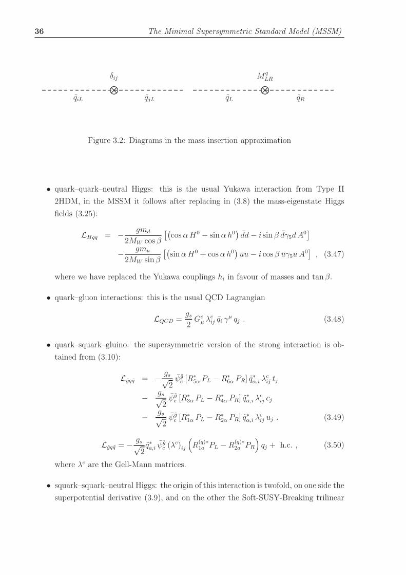
36 The Minimal Supersymmetric Standard Model (MSSM)
qiL qjL
⊗
δij
qL qR
⊗
M qLR
Figure 3.2: Diagrams in the mass insertion approximation
• quark–quark–neutral Higgs: this is the usual Yukawa interaction from Type II
2HDM, in the MSSM it follows after replacing in (3.8) the mass-eigenstate Higgs
fields (3.25):
LHqq = − gmd
2MW cosβ
[(
cosαH0 − sinαh0)
dd− i sin β dγ5dA0]
− gmu
2MW sin β
[(
sinαH0 + cosαh0)
uu− i cosβ uγ5uA0]
, (3.47)
where we have replaced the Yukawa couplings hi in favour of masses and tanβ.
• quark–gluon interactions: this is the usual QCD Lagrangian
LQCD =gs2Gcµ λ
cij qi γ
µ qj . (3.48)
• quark–squark–gluino: the supersymmetric version of the strong interaction is ob-
tained from (3.10):
Lgqq = − gs√2ψgc [R∗
5α PL −R∗6α PR] q∗α,i λ
cij tj
− gs√2ψgc [R∗
3α PL − R∗4α PR] q∗α,i λ
cij cj
− gs√2ψgc [R∗
1α PL − R∗2α PR] q∗α,i λ
cij uj . (3.49)
Lgqq = − gs√2q∗a,i ψ
gc (λc)ij
(
R(q)∗1a PL −R(q)∗
2a PR
)
qj + h.c. , (3.50)
where λc are the Gell-Mann matrices.
• squark–squark–neutral Higgs: the origin of this interaction is twofold, on one side the
superpotential derivative (3.9), and on the other the Soft-SUSY-Breaking trilinear
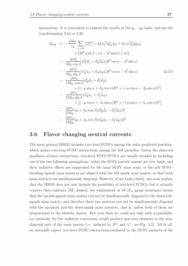
3.6 Flavor changing neutral currents 37
interactions. It is convenient to express the results in the qL− qR basis, and use the
transformation 3.44 or 3.38.
Lhqq = −gMZ
cθ
∑
i=u,d
[
(T iL3 −Qisθ2)q∗iLqiL +Qisθ
2q∗iRqiR]
×(
H0 cos(β + α)− h0 sin(β + α))
− gm2d
MW cosβ(d∗LdL + d∗RdR)(H0 cosα− h0 sinα)
− gm2u
MW sin β(u∗LuL + u∗RuR)(H0 cosα− h0 sinα) (3.51)
− gmd
2MW cosβ(d∗RdL + d∗LdR)
×[
(−µ sinα + Ad cosα)H0 + (−µ cosα− Ad sinα)h0]
− gmu
2MW sin β(u∗RuL + u∗LuR)
×[
(−µ cosα+ Au sinα)H0 + (+µ sinα + Au cosα)h0]
− igmu
2MW(µ+ Ad tan β)(d∗RdL − d∗LdR)A0
− igmu
2MW(µ+ Au cot β)(u∗RuL − u∗LuR)A0
3.6 Flavor changing neutral currents
The most general MSSM includes tree-level FCNCs among the extra predicted particles,
which induce one-loop FCNC interactions among the SM particles. Given the observed
smallness of these interactions, tree-level SUSY FCNCs are usually avoided by including
one of the two following assumptions: either the SUSY particle masses are very large, and
their radiative effects are suppressed by the large SUSY mass scale; or the soft SUSY-
breaking squark mass matrices are aligned with the SM quark mass matrix, so that both
mass matrices are simultaneously diagonal. However, if one looks closely, one soon realizes
that the MSSM does not only include the possibility of tree-level FCNCs, but it actually
requires their existence [93]. Indeed, the requirement of SU(2)L gauge invariance means
that the up-left-squark mass matrix can not be simultaneously diagonal to the down-left-
squark mass matrix, and therefore these two matrices can not be simultaneously diagonal
with the up-quark and the down-quark mass matrices, that is, unless both of them are
proportional to the identity matrix. But even then we could not take such a possibility
too seriously, for the radiative corrections would produce non-zero elements in the non-
diagonal part of the mass matrix (i.e. induced by H± and χ±, see Fig. 3.3). All in all,
we naturally expect tree-level FCNC interactions mediated by the SUSY partners of the
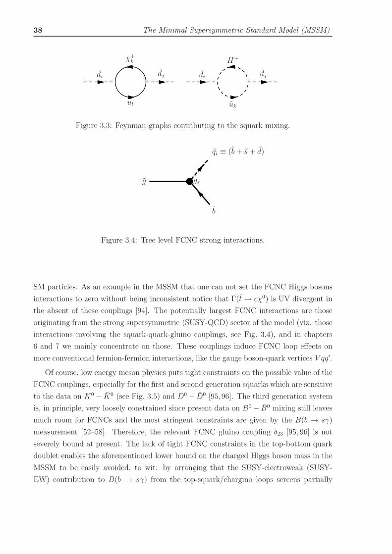
38 The Minimal Supersymmetric Standard Model (MSSM)
di
ul
χ+k
dj di
uk
H+
dj
Figure 3.3: Feynman graphs contributing to the squark mixing.
g
b
qi ≡ (b+ s+ d)
gs
Figure 3.4: Tree level FCNC strong interactions.
SM particles. As an example in the MSSM that one can not set the FCNC Higgs bosons
interactions to zero without being inconsistent notice that Γ(t→ cχ0) is UV divergent in
the absent of these couplings [94]. The potentially largest FCNC interactions are those
originating from the strong supersymmetric (SUSY-QCD) sector of the model (viz. those
interactions involving the squark-quark-gluino couplings, see Fig. 3.4), and in chapters
6 and 7 we mainly concentrate on those. These couplings induce FCNC loop effects on
more conventional fermion-fermion interactions, like the gauge boson-quark vertices V qq′.
Of course, low energy meson physics puts tight constraints on the possible value of the
FCNC couplings, especially for the first and second generation squarks which are sensitive
to the data on K0 − K0 (see Fig. 3.5) and D0− D0 [95,96]. The third generation system
is, in principle, very loosely constrained since present data on B0− B0 mixing still leaves
much room for FCNCs and the most stringent constraints are given by the B(b → sγ)
measurement [52–58]. Therefore, the relevant FCNC gluino coupling δ23 [95, 96] is not
severely bound at present. The lack of tight FCNC constraints in the top-bottom quark
doublet enables the aforementioned lower bound on the charged Higgs boson mass in the
MSSM to be easily avoided, to wit: by arranging that the SUSY-electroweak (SUSY-
EW) contribution to B(b → sγ) from the top-squark/chargino loops screens partially
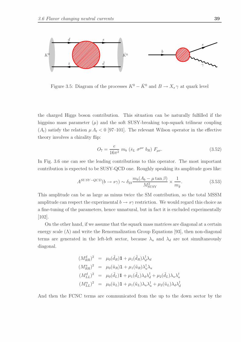
3.6 Flavor changing neutral currents 39
d
ds
s
K0 K0b
s
γ
Figure 3.5: Diagram of the processes K0 − K0 and B → Xs γ at quark level
the charged Higgs boson contribution. This situation can be naturally fulfilled if the
higgsino mass parameter (µ) and the soft SUSY-breaking top-squark trilinear coupling
(At) satisfy the relation µAt < 0 [97–101]. The relevant Wilson operator in the effective
theory involves a chirality flip:
O7 =e
16π2mb (sL σ
µν bR) Fµν . (3.52)
In Fig. 3.6 one can see the leading contributions to this operator. The most important
contribution is expected to be SUSY-QCD one. Roughly speaking its amplitude goes like:
ASUSY−QCD(b→ sγ) ∼ δ23mb(Ab − µ tanβ)
M2SUSY
× 1
mg. (3.53)
This amplitude can be as large as minus twice the SM contribution, so the total MSSM
amplitude can respect the experimental b→ sγ restriction. We would regard this choice as
a fine-tuning of the parameters, hence unnatural, but in fact it is excluded experimentally
[102].
On the other hand, if we assume that the squark mass matrices are diagonal at a certain
energy scale (Λ) and write the Renormalization Group Equations [93], then non-diagonal
terms are generated in the left-left sector, because λu and λd are not simultaneously
diagonal.
(MdRR)2 = µ0(dR)1+ µ1(dR)λ†dλd
(MuRR)2 = µ0(uR)1+ µ1(uR)λ†uλu
(MdLL)
2 = µ0(dL)1 + µ1(dL)λdλ†d + µ2(dL)λuλ
†u
(MuLL)
2 = µ0(uL)1+ µ1(uL)λuλ†u + µ2(uL)λdλ
†d
And then the FCNC terms are communicated from the up to the down sector by the

40 The Minimal Supersymmetric Standard Model (MSSM)
bR W+
t
sLbL
γ
mb
bR H+
t
sL
γ
bR χ−
tL
sL
tR
γ
mt(At − µ/ tanβ)⊗
bR
bR
sL
bL
sL
γ
mg
mb(Ab − µ tanβ) δ23⊗ ⊗
bR g
bL
sL
sL
bL
γ
δ23⊗
mb
Figure 3.6: Leading contributions to the b→ sγ Wilson operator O7.
3.6 Flavor changing neutral currents 41
CKM matrix, due to the SU(2) gauge invariant:
(MdLL)2 = V †
CKM × (MuLL)
2 × VCKM (3.54)
The FCNC gluino interactions also induce large contributions to B(b → sγ), see
Fig. 3.6. It should be noted however that the leading contributions to the V qq′ FCNC
interactions from the third quark generation correspond to a double insertion term, in
which the squarks propagating in the loop suffer a double mutation: a flavor conversion
and a chirality transition. This fact has been demonstrated in the B(b→ sγ) observable
itself [103], as well as in the FCNC rare decay width Γ(t → cg) [43]. As a consequence,
the loose limits on the third generation FCNC interactions derived under the assumption
that the leading terms contributing to b→ sγ correspond to the single particle insertion
approximation [95, 96] are not valid and more complex expressions must be taken into
account [104].
The FCNC effects in the K0−K0 system can be described with an effective Lagrangian
with a mass matrix as:(
m2K A
A m2K
)
⇒ diagonalize⇒ m2K1,2
= m2K ± A (3.55)
so the signal of FCNC can determined by the mass difference of the eigenstates:
∆mK ≡ |mK1−mK2
| (3.56)
In contrast the experimental signal for b→ sγ is directly its branching ratio. The exper-
imental measurements are [19, 53–55,57]:
B(b→ sγ) = (3.3± 0.4)× 10−4 (3.57)
∆mK = (3.483± 0.006)× 10−12 MeV (ds↔ ds) (3.58)
mK = 497.648± 0.022MeV
∆mD < 4.6× 10⁻¹¹ MeV (cu↔ cu) (3.59)
mD = 1864.6± 0.5MeV
∆mB = (3.304± 0.046)× 10−10 MeV (bd↔ bd) (3.60)
mB = 5279.4± 0.5MeV
that translated to δij restrictions they read:
δ12 . .1√mumc/500GeV
δ13 . .098√mumt/500GeV
δ23 . 8.2mcmt/(500GeV)2
(3.61)
42 The Minimal Supersymmetric Standard Model (MSSM)
3.7 MSSM parametrization
3.7.1 MSSM parameters
Since SUSY is a broken symmetry we have to deal with a plethora of Soft-SUSY-Breaking
parameters, namely
• tanβ,
• masses for Left- and Right-chiral sfermions,
• a mass for the Higgs sector,
• gaugino masses,
• triple scalar couplings for squarks and Higgs.
This set of parameters is often simplified to allow a comprehensive study. Most of
these simplifications are based on some universality assumption at the unification scale.
In minimal supergravity (mSUGRA) all the parameters of the MSSM are computed from
a restricted set of parameters at the Unification scale, to wit: tan β; a common scalar
mass m0; a common fermion mass for gauginos m1/2; a common trilinear coupling for all
sfermions A0; and the higgsino mass parameter µ. Then one computes the running of
each one of these parameters down to the EW scale, using the Renormalization Group
Equations (RGE), and the full spectrum of the MSSM is found.
We will not restrict ourselves to a such simplified model. As stated in the introduc-
tion we treat the MSSM as an effective Lagrangian, to be embedded in a more general
framework that we don’t know about. This means that essentially all the parameters
quoted above are free. However for the kind of studies we have performed there is an
implicit asymmetry of the different particle generations. We are mostly interested in the
phenomenology of the third generation, thus we will treat top and bottom supermultiplet
as distinguished from the rest. This approach is well justified by the great difference of
the Yukawa couplings of top and bottom with respect to the rest of fermions. We are
mainly interested on effects on the Higgs sector, so the smallness of the Yukawa couplings
of the first two generations will result on small effects in our final result. We include them,
though, in the numerical analysis and the numerical dependence is tested. On the other
hand, if we suppose that there is unification at some large scale, at which all sfermions
have the same mass, and then evolve these masses to the EW scale, then the RGE have
great differences [12]. Slepton RGE are dominated by EW gauge interactions, 1st and 2nd
generation squarks RGE are dominated by QCD, and for the 3rd generation squarks there
3.7 MSSM parametrization 43
is an interplay between QCD and Yukawa couplings. Also, as a general rule, the gauge
contribution to the RGE equations of left- and right-handed squark masses are similar,
so when Yukawa couplings are not important they should be similar at the EW scale.
With the statement above in mind we can simplify the MSSM spectrum by taking
an unified parametrization for 1st and 2nd generation squarks (same for sleptons). As
we have seen in Sect. 3.4.3 we will use: a common mass1 for uL and qR (mu); an unified
trilinear coupling Au for 1st and 2nd generation; a common mass for all νL and lR (mτ );
and a common trilinear coupling Aτ .
For the third generation we will use different trilinear couplings At and Ab, as these
can play an important role in the kind of processes we are studying (see chapter 6 and
7). Stop masses can present a large gap (due to its Yukawa couplings), being the right-
handed stop the lightest one. We will use a common mass for both chiral sbottoms, which
we parametrize with the lightest sbottom mass (mb), and the lightest stop quark mass
(mt), as the rest of mass inputs in this sector. This parametrization is useful in processes
where squarks only appear as internal particles in the loops (such as the ones studied in
chapters 6 and 7), as one-loop corrections to these parameters would appear as two-loop
effects in the process subject of study. Gluino mass (mg), on the other hand, is let free.
For the Higgs sector two choices are available, we can use the pseudoscalar mass mA0 ,
or the charged Higgs mass mH±. Both choices are on equal footing. As the neutral Higgs
particles are the main element for most of our studies we shall use its mass as input
parameter in most of our work.
Standard model parameters are well known, we will use present determinations of EW
observables [19]
MZ = 91.1899± 0.0021GeV
MW = 80.418± 0.054GeV
GF = (1.16639± 0.00001)× 10−5 GeV−2
α−1em(MZ) = 128.896± 0.090
(3.62)
QCD related observables are not so precise. On the other hand as the main results are
not affected by specific value of these observables we will use the following ones
mt = 175GeV
mb = 5GeV
αs(MZ) = 0.11 (3.63)
1Note that after diagonalization of the squark mass matrix the physical masses will differ slightly.
44 The Minimal Supersymmetric Standard Model (MSSM)
3.7.2 Constraints
The MSSM reproduces the behaviour of the SM up to energy scales probed so far [105].
Obviously this is not for every point of the full parameter space!
There exists direct limits on sparticle masses based on direct searches at the high
energy colliders (LEP II, SLC, Tevatron). Although hadron colliders can achieve larger
center of mass energies than e+e− ones, their samples contain large backgrounds that
make the analysis more difficult. This drawback can be avoided if the ratio signal-to-
background is improved, in fact they can be used for precision measurements of “known”
observables (see e.g. [17]). e+e− colliders samples are more clean, and they allow to put
absolute limits on particle masses in a model independent way.
No significant evidence for a Higgs signal has been detected at LEP [106]. As a result,
one can obtain bounds on the possible MSSM Higgs parameters. These limits are often
displayed in the mA0–tan β plane, see Fig. 3.7, although there is additional dependence
on various MSSM parameters that effect the radiative corrections to the Higgs masses
as discussed above. In representative scans of the MSSM parameters, the LEP Higgs
Working Group [106] finds that mh0 > 91.0 GeV and mA0 > 91.9 GeV at 95% CL.
These limits actually correspond to the large tanβ region in which Zh0 production is
suppressed, as shown in Fig. 3.7. In this case, the quoted Higgs limits arise as a result
of the non-observation of h0A0 and H0A0 production. As tan β is lowered, the limits on
mh0 and mA0 become more stringent. In this regime, the h0A0 production is suppressed
while the Zh0 production rate approaches its SM value. Thus, in this case, the SM Higgs
limit applies (mh0 & 114GeV [19]) as shown in Fig. 3.7(a). The precise region of MSSM
Higgs parameter space that is excluded depends on the values of the MSSM parameters
that control the Higgs mass radiative corrections. For example, a conservative exclusion
limit is obtained in the maximal mixing scenario, since in this case the predicted value
of mh0 as a function of mA0 and tan β is maximal (with respect to changes in the other
MSSM parameters). The excluded regions of the MSSM Higgs parameter space based
on the maximal mixing benchmark scenario of Ref. [107], are shown in Fig. 3.7, and
correspond to the exclusion of the range 0.5 < tanβ < 2.4 at the 95% CL. However, the
tanβ exclusion region can still be significantly reduced (even to the point of allowing all
tanβ values) by, e.g., taking MSUSY = 2 TeV and mt = 180 GeV, see Fig 3.8 (which
still lies within the error bars of the experimentally measured value), and allowing for the
theoretical uncertainty in the prediction of mh0max [108].
Similarly, no evidence for the charged Higgs boson has yet been found. The LEP
Higgs Working Group quotes a limit of mH± > 78.6 GeV at 95% CL [109], which holds
for a more general non-supersymmetric two-Higgs doublet model and assumes only that

3.7 MSSM parametrization 45
1
10
0 20 40 60 80 100 120 140
1
10
LEP 88-209 GeV Preliminary
mh° (GeV/c2)
tanβ
Excludedby LEP
TheoreticallyInaccessible
mh°-max
1
10
0 100 200 300 400 500
1
10
LEP 88-209 GeV Preliminary
mA° (GeV/c2)
tanβ
Excludedby LEP
mh°-max
MSUSY=1 TeVM2=200 GeVµ=-200 GeVmgluino=800 GeVStop mix: Xt=2MSUSY
Figure 3.7: LEP2 contours of the 95% CL exclusion limits for MSSM Higgs sector pa-
rameters as a function of tan β and (a) mh0 and (b) mA0 (in GeV), taken from Ref. [106].
The contours shown have been obtained for MSSM Higgs parameters chosen according to
the maximal mixing benchmark of Ref. [107].
70 80 90 100 110 120 130mh [GeV]
0.5
1.0
1.5
2.0
2.5
3.0
3.5
4.0
4.5
5.0
tan
β
mt = 174.3 GeVmt = 179.4 GeVmt = 184.5 GeV
HHW, MSUSY = 1000 GeV
µ = − 100 GeV
Figure 3.8: Theoretically exclusion limits as in Fig. 3.7 for three different values of the
top-quark mass, mt = 174.3, 179.4, 184.5GeV. Taken from Ref. [108]
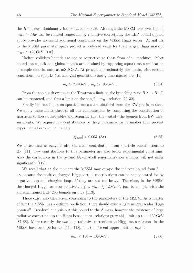
46 The Minimal Supersymmetric Standard Model (MSSM)
the H+ decays dominantly into τ+ντ and/or cs. Although the MSSM tree-level bound
mH± ≥ MW can be relaxed somewhat by radiative corrections, the LEP bound quoted
above provides no useful additional constraints on the MSSM Higgs sector. Actual fits
to the MSSM parameter space project a preferred value for the charged Higgs mass of
mH± ≃ 120GeV [110].
Hadron colliders bounds are not so restrictive as those from e+e− machines. Most
bounds on squark and gluino masses are obtained by supposing squark mass unification
in simple models, such as mSUGRA. At present approximately the limits, with certain
conditions, on squarks (1st and 2nd generation) and gluino masses are [19]
mq > 250GeV , mg > 195GeV . (3.64)
From the top quark events at the Tevatron a limit on the branching ratio B(t→ H+ b)
can be extracted, and thus a limit on the tanβ −mH± relation [20, 32].
Finally indirect limits on sparticle masses are obtained from the EW precision data.
We apply these limits through all our computations by computing the contribution of
sparticles to these observables and requiring that they satisfy the bounds from EW mea-
surements. We require new contributions to the ρ parameter to be smaller than present
experimental error on it, namely
|δρnew| < 0.003 (3σ) . (3.65)
We notice that as δρnew is also the main contribution from sparticle contributions to
∆r [111], new contributions to this parameter are also below experimental constrains.
Also the corrections in the α- and GF -on-shell renormalization schemes will not differ
significantly [112].
We recall that at the moment the MSSM may escape the indirect bound from b →s γ because the positive charged Higgs virtual contributions can be compensated for by
negative stop and chargino loops, if they are not too heavy. Therefore, in the MSSM
the charged Higgs can stay relatively light, mH± & 120GeV , just to comply with the
aforementioned LEP 200 bounds on mA0 [113].
There exist also theoretical constrains to the parameters of the MSSM. As a matter
of fact the MSSM has a definite prediction: there should exist a light neutral scalar Higgs
boson h0. Tree-level analysis put this bound to the Z mass, however the existence of large
radiative corrections to the Higgs bosons mass relations grow this limit up to ∼ 130GeV
[87, 88]. More recently the two-loop radiative corrections to Higgs mass relations in the
MSSM have been performed [114–118], and the present upper limit on mh0 is
mh0 ≤ 130− 135GeV . (3.66)

3.7 MSSM parametrization 47
Of course if the MSSM is extended in some way this limit can be evaded, though not to
values larger of ∼ 200GeV [119,120].
Another theoretical constraint is the necessary condition (3.41) on squark trilinear
coupling (A) to avoid colour-breaking minima. This constraint is easily implemented
when the A parameters are taken as inputs, but if we choose a different set of inputs
(such as the mixing angle θq) then it constrains the parameter space in a non-trivial way.
Whatever the spectrum of the MSSM is, it should comply with the benefits that SUSY
introduces into the SM which apply if the following condition is fulfilled:
MSUSY . O(1 TeV) . (3.67)
If supersymmetric particles have masses heavier than the TeV scale then problems with
GUT’s appear. This statement does not mean that SUSY would not exist, but that then
the SM would not gain practical benefit from the inclusion of SUSY.
A similar upper bound is obtained when making cosmological analyses, in these type
of analyses one supposes the neutralino to be part of the cold dark matter of the universe,
and requires its annihilation rate to be sufficiently small to account for the maximum
of cold dark matter allowed for cosmological models, while at the same time sufficiently
large so that its presence does not becomes overwhelming. Astronomical observations also
restrict the parameters of SUSY models, usually in the lower range of the mass parameters
(see e.g. [121–123]).
For the various RGE analyses to hold the couplings of the MSSM should be pertur-
bative all the way from the unification scale down to the EW scale. This implies, among
other restrictions, that top and bottom quark Yukawa couplings should be below certain
limits (h2t,b/4π < 1). In terms of tan β this amounts it to be confined in the approximate
interval
1 < tanβ . 70 . (3.68)
There are additional phenomenological restrictions that bring the lower bound on tanβ
to roughly 2.4 for the so-called maximal m0h scenario, and 10.5 for the so-called no mixing
scenario [113], the upper bound being the same [11].
In the MSSM case we use the more restrictive limits (3.68), see Fig. 3.7, whereas in
the 2HDM model the lower limit can be smaller as shown in (2.43). Any deviation from
this framework of restrictions will only be for demonstrational purpouses, and will be
explicitly quoted in the text.
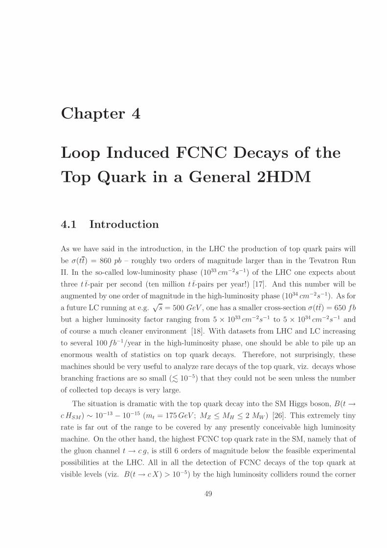
Chapter 4
Loop Induced FCNC Decays of the
Top Quark in a General 2HDM
4.1 Introduction
As we have said in the introduction, in the LHC the production of top quark pairs will
be σ(tt) = 860 pb – roughly two orders of magnitude larger than in the Tevatron Run
II. In the so-called low-luminosity phase (1033 cm−2s−1) of the LHC one expects about
three t t-pair per second (ten million t t-pairs per year!) [17]. And this number will be
augmented by one order of magnitude in the high-luminosity phase (1034 cm−2s−1). As for
a future LC running at e.g.√s = 500 GeV , one has a smaller cross-section σ(tt) = 650 fb
but a higher luminosity factor ranging from 5 × 1033 cm−2s−1 to 5 × 1034 cm−2s−1 and
of course a much cleaner environment [18]. With datasets from LHC and LC increasing
to several 100 fb−1/year in the high-luminosity phase, one should be able to pile up an
enormous wealth of statistics on top quark decays. Therefore, not surprisingly, these
machines should be very useful to analyze rare decays of the top quark, viz. decays whose
branching fractions are so small (. 10−5) that they could not be seen unless the number
of collected top decays is very large.
The situation is dramatic with the top quark decay into the SM Higgs boson, B(t→cHSM) ∼ 10−13 − 10−15 (mt = 175GeV ; MZ ≤ MH ≤ 2 MW ) [26]. This extremely tiny
rate is far out of the range to be covered by any presently conceivable high luminosity
machine. On the other hand, the highest FCNC top quark rate in the SM, namely that of
the gluon channel t → c g, is still 6 orders of magnitude below the feasible experimental
possibilities at the LHC. All in all the detection of FCNC decays of the top quark at
visible levels (viz. B(t→ cX) > 10−5) by the high luminosity colliders round the corner
49

50 Loop Induced FCNC Decays of the Top Quark in a General 2HDM
(especially LHC and LC) seems doomed to failure in the absence of new physics. Thus
the possibility of large enhancements of some FCNC channels up to the visible threshold,
particularly within the context of the general 2HDM and the MSSM, should be very
welcome. Unfortunately, although the FCNC decay modes into electroweak gauge bosons
Vew = W,Z may be enhanced a few orders of magnitude, it proves to be insufficient to raise
the meager SM rates mentioned before up to detectable limits, and this is true both in the
2HDM – where B(t→ Vew c) < 10−6 [24] – and in the MSSM – where B(t→ Vew c) < 10−7
except in highly unlikely regions of the MSSM parameter space [124]1. In this respect
it is a lucky fact that these bad news need not to apply to the gluon channel, which
could be barely visible (B(t→ g c) . 10−5) both in the MSSM [42,43] and in the general
2HDM [24]. But, most significant of all, they may not apply to the non-SM Higgs boson
channels t → (h0, H0, A0) + c either. As we shall show in the sequel, these Higgs decay
channels of the top quark could lie above the visible threshold for a parameter choice
made in perfectly sound regions of parameter space!
While a systematic discussion of these “gifted” Higgs channels was made in Ref. [43]
for the MSSM case and in other models2, to the best of our knowledge there is no similar
study in the general 2HDM. And we believe that this study is necessary, not only to assess
what are the chances to see traces of new (renormalizable) physics in the new colliders
round the corner but also to clear up the nature of the virtual effects; in particular to dis-
entangle whether the origin of the hypothetically detected FCNC decays of the top quark
is ultimately triggered by SUSY or by some alternative, more generic, renormalizable
extension of the SM such as the 2HDM or generalizations thereof. Of course the alleged
signs of new physics could be searched for directly through particle tagging, if the new
particles were not too heavy. However, even if accessible, the corresponding signatures
could be far from transparent. In contrast, the indirect approach based on the FCNC
processes has the advantage that one deals all the time with the dynamics of the top
quark. Thus by studying potentially new features beyond the well-known SM properties
of this quark one can hopefully uncover the existence of the underlying new interactions.
1Namely, regions in which there are wave-function renormalization thresholds due to (extremely for-
tuitous!) sharp coincidences between the sum of the sparticle masses involved in the self-energy loops
and the top quark mass. See e.g. Ref. [125] for similar situations already in the conventional t → W b
decay within the MSSM. In our opinion these narrow regions should not be taken too seriously.2Preliminary SUSY analysis of the Higgs channels are given in [126], but they assume the MSSM Higgs
mass relations at the tree-level. Therefore these are particular cases of the general MSSM approach given
in [43]. Studies beyond the MSSM (e.g. including R-parity violation) and also in quite different contexts
from the present one are available in the literature, see e.g. [127].

4.2 Relevant fields and interactions in the 2HDM 51
4.2 Relevant fields and interactions in the 2HDM
We will mainly focus our interest on the loop induced FCNC decays
t→ c h (h = h0, H0, A0) , (4.1)
in which any of the three possible neutral Higgs bosons from a general 2HDM can be
in the final state. However, as a reference we shall compare throughout our analysis the
Higgs channels with the more conventional gluon channel
t→ c g . (4.2)
Although other quarks could participate in the final state of these processes, their contri-
bution is obviously negligible – because it is further CKM-suppressed. The lowest order
diagrams entering these decays are one-loop diagrams in which Higgs, quarks, gauge and
Goldstone bosons – in the Feynman gauge – circulate around. While the diagrams for the
decays (4.1) are depicted in Fig. 4.1, the ones for the decay (4.2) are not shown [24].
We wish to concentrate here on Type I and Type II models of a sufficiently generic
nature, to wit, those which are characterized by the following set of free parameters:
(mh0 , mH0 , mA0, mH± , tanα, tanβ) , (4.3)
tan β is a key parameter in our analysis. The numerical analysis that we perform in the
next section does not depend in any essential way on the simplification λ5 = λ6,(2.8). In
essence we have just traded λ5 for m2A0 in these rules and so by varying with respect to
mA0 we do explore most of the quantitative potential of the general 2HDM.
Since we shall perform our calculation in the on-shell scheme, we understand that the
physical inputs are given by the electromagnetic coupling and the physical masses of all
the particles:
(e,MW ,MZ , mh0, mH0 , mA0 , mH±, mf ) . (4.4)
The remaining parameters, except the Higgs mixing angles, are understood to be given in
terms of the latter, e.g. the SU(2) gauge coupling appearing in the previous formulae and
in Table 2.1 is given by g = e/sw , where the sinus of the weak mixing angle is defined
through s2w = 1−M2
W/M2Z . It should be clear that, as there are no tree-level FCNC decays
of the top quark, there is no need to introduce counterterms for the physical inputs in
this calculation. In fact, the calculation is carried out in lowest order (“tree level”) with
respect to the effective tch and tcg couplings and so the sum of all the one-loop diagrams
(as well as of certain subsets of them) should be finite in a renormalizable theory, and
indeed it is.

52 Loop Induced FCNC Decays of the Top Quark in a General 2HDMPSfrag repla ements H�; G�t hW� dd
PSfrag repla ementsH�; G� t hW� d H�; G�H�; G�PSfrag repla ementsH�; G� t
hW� ddPSfrag repla ementsH�; G� t
hW�dH�; G�PSfrag repla ementsH�; G� t
hW�d H�; G�PSfrag repla ementsH�; G� t hW�W�d
PSfrag repla ements H�; G�t hW� dPSfrag repla ementsH�; G� t h W�dFigure 4.1: One-loop vertex diagrams contributing to the FCNC top quark decays (4.1).
Shown are the vertices and mixed self-energies with all possible contributions from the SM
fields and the Higgs bosons from the general 2HDM. The Goldstone boson contributions
are computed in the Feynman gauge.
4.3 Numerical analysis
From the previous interaction Lagrangians and Feynman rules it is now straightforward
to compute the loop induced FCNC rates for the decays (4.1) and (4.2). We shall refrain
from listing the lengthy analytical formulae as the computation is similar to the one
reported in great detail in Ref. [43]. Therefore, we will limit ourselves to exhibit the final
numerical results. The fiducial ratio on which we will apply our numerical computation
is the following:
Bj(t→ h+ c) =Γj(t→ h+ c)
Γ(t→W+ + b) + Γj(t→ H+ + b), (4.5)

4.3 Numerical analysis 53
for each Type j = I, II of 2HDM and for each neutral Higgs boson h = h0, H0, A0. While
this ratio is not the total branching fraction, it is enough for most practical purposes and
it is useful in order to compare with previous results in the literature. Notice that for
mH± > mt (the most probable situation for Type II 2HDM’s, see below) the ratio (4.5)
reduces to Bj(t → h + c) = Γj(t → h + c)/Γ(t → W+ + b), which is the one that
we used in Ref. [43]. It is understood that Γj(t → h + c) above is computed from the
one-loop diagrams in Fig. 4.1, with all quark families summed up in the loop. Therefore,
consistency in perturbation theory requires to compute Γ(t→W++b) and Γ(t→ H++b)
in the denominator of (4.5) only at the tree-level (for explicit expressions see e.g. [20]).
As mentioned in Sec. 2, we wish to compare our results for the Higgs channels (4.1) with
those for the gluon channel (4.2), so that we similarly define
Bj(t→ g + c) =Γj(t→ g + c)
Γ(t→W+ + b) + Γj(t→ H+ + b). (4.6)
We have performed a fully-fledged independent analytical and numerical calculation of
Γj(t → g + c) at one-loop in the context of 2HDM I and II. Where there is overlapping,
we have checked the numerical results of Ref. [24], but we point out that they agree with
us only if Γ(t→ H+ + b) is included in the denominator of eq. (4.6), in contrast to what
is asserted in that reference in which B(t → g + c) is defined without the charged Higgs
channel contribution.
We have performed part of the analytical calculation of the diagrams for both pro-
cesses (4.1) and (4.2) by hand and we have cross-checked our results with the help of
the numeric and algebraic programs FeynArts, FormCalc and LoopTools [128–130], with
which we have completed the rest of the calculation. In particular, the cancellation of
UV divergences in the total amplitudes was also verified by hand. In addition we have
checked explicitly the gauge invariance of the total analytical amplitude for the pro-
cess (4.2), which is a powerful test. And we have confirmed that our code reproduces the
SUSY Higgs contribution of Ref. [43] when we turn on the MSSM Higgs mass relations.
As mentioned above, a highly relevant parameter is tanβ, which must be restricted
to the approximate range (2.43) in perturbation theory3. It is to be expected from the
various couplings involved in the processes under consideration that the low tanβ region
could be relevant for both the Type I and Type II 2HDM’s. In contrast, the high tanβ
region is only potentially important for the Type II. However, the eventually relevant
3Some authors [131] claim that perturbativity allows tanβ to reach values of order 100 and beyond,
and these are still used in the literature. We consider it unrealistic and we shall not choose tan β outside
the interval (2.43). Plots versus tanβ, however, will indulge larger values just to exhibit the dramatic
enhancements of our FCNC top quark rates.

54 Loop Induced FCNC Decays of the Top Quark in a General 2HDM
regions of parameter space are also determined by the value of the mixing angle α, as we
shall see below.
Of course there are several restrictions that must be respected by our numerical anal-
ysis, see 2.4, as the ρ-parameter restriction, (2.44), and the b → sγ restriction, (2.45).
With the charge Higgs boson mass restrictions in section 2.4 4 in principle the top quark
decay t → H+ + b is still possible in 2HDM I; but also in 2HDM II, if mH± lies near
the lowest end of the previous bound, and in this case that decay can contribute to the
denominator of eqs. (4.5)-(4.6).
The combined set of independent conditions turns out to be quite effective in narrowing
down the permitted region in the parameter space, as can be seen in Figs. 4.2-4.5 where
we plot the fiducial FCNC rates (4.5)-(4.6) versus the parameters (4.3). The cuts in some
of these curves just reflect the fact that at least one of these conditions is not fulfilled.
After scanning the parameter space, we see in Figs. 4.2-4.3 that the 2HDM I (resp.
2HDM II) prefers low values (resp. high values) of tanα and tan β for a given channel,
e.g. t → h0 c. Therefore, the following choice of mixing angles will be made to optimize
the presentation of our numerical results:
2HDM I : tanα = tanβ = 1/4 ;
2HDM II : tanα = tanβ = 50 . (4.7)
We point out that, for the same values of the masses, one obtains the same maximal
FCNC rates for the alternative channel t → H0 c provided one just substitutes α →π/2− α. Equations (4.7) define the eventually relevant regions of parameter space and,
as mentioned in section 2.4, depend on the values of the mixing angles α and β, namely
β ≃ α ≃ 0 for Type I and β ≃ α ≃ π/2 for Type II.
Due to the α → π/2 − α symmetry of the maximal rates for the CP-even Higgs
channels, it is enough to concentrate the numerical analysis on one of them, but one has
to keep in mind that the other channel yields the same rate in another region of parameter
space. Whenever a mass has to be fixed, we choose conservatively the following values
for both models:
mh0 = 100GeV , mH0 = 150GeV , mA0 = mH± = 180GeV . (4.8)
Also for definiteness, we take the following values for some relevant SM parameters in our
calculation:
mt = 175GeV , mb = 5GeV , αs(mt) = 0.11 , Vcb = 0.040 , (4.9)
4At the time of this work this restriction was mH± > (165 − 200) GeV for virtually any tanβ & 1
[60, 80].

4.3 Numerical analysis 55
−0.5 −0.25 0 0.25 0.5α/π
1e−13
1e−12
1e−11
1e−10
1e−09
1e−08
h0
H0
g
Type I
PSfrag repla ements (a)10
−110
010
110
2
tan(β)
1e−16
1e−15
1e−14
1e−13
1e−12
1e−11
1e−10
1e−09
1e−08
1e−07
1e−06Type I
PSfrag repla ements (b)Figure 4.2: Evolution of the FCNC top quark fiducial ratios (4.5)-(4.6) in Type I 2HDM
versus: (a) the mixing angle α in the CP-even Higgs sector, in units of π; (b) tan β. The
values of the fixed parameters are as in eqs. (4.7) and (4.8).
and the remaining ones are as in [75]. Notice that our choice of mA0 prevents the decay
t→ A0 c from occurring, and this is the reason why it does not appear in Figs. 4.2- 4.3.
The variation of the results with respect to the masses is studied in Figs. 4.4-4.5. In
particular, in Fig. 4.4 we can see the (scanty) rate of the channel t → A0 c when it is
kinematically allowed. In general the pseudoscalar channel is the one giving the skimpiest
FCNC rate. This is easily understood as it is the only one that does not have trilinear
couplings with the other Higgs particles (Cf. Table 2.1). While it does have trilinear
couplings involving Goldstone bosons, these are not enhanced. The crucial role played by
the trilinear Higgs self-couplings in our analysis cannot be underestimated as they can
be enhanced by playing around with both (large or small) tanβ and also with the mass
splittings among Higgses. This feature is particularly clear in Fig. 4.4a where the rate of
the channel t→ h0 c is dramatically increased at large mA0 , for fixed values of the other
parameters and preserving our list of constraints. Similarly would happen for t → H0 c
in the corresponding region α→ π/2− α.
From Figs. 4.2a and 4.2b it is pretty clear that the possibility to see FCNC decays
of the top quark into Type I Higgs bosons is plainly hopeless even in the most favorable
regions of parameter space – the lowest (allowed) tanβ end. In fact, the highest rates
remain neatly down 10−6, and therefore they are (at least) one order of magnitude below
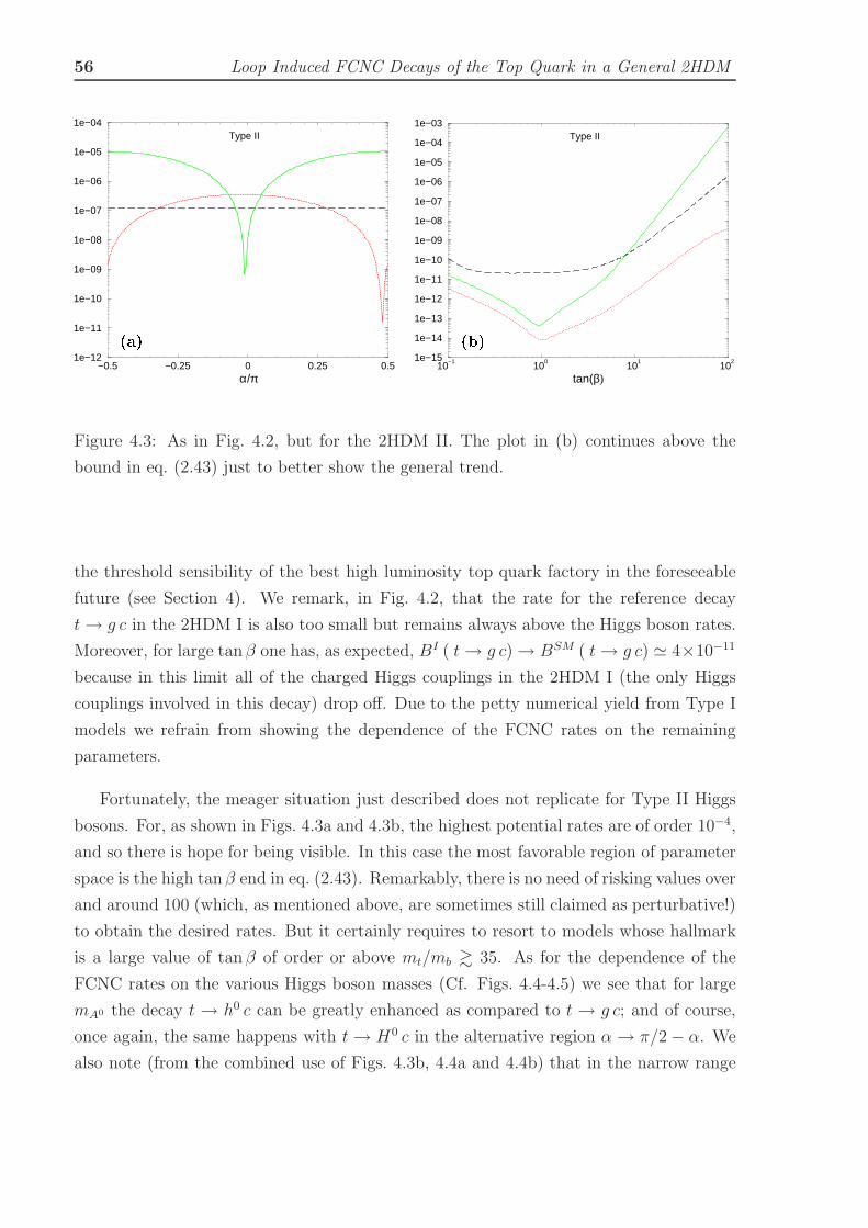
56 Loop Induced FCNC Decays of the Top Quark in a General 2HDM
−0.5 −0.25 0 0.25 0.5α/π
1e−12
1e−11
1e−10
1e−09
1e−08
1e−07
1e−06
1e−05
1e−04Type II
PSfrag repla ements (a)10
−110
010
110
2
tan(β)
1e−15
1e−14
1e−13
1e−12
1e−11
1e−10
1e−09
1e−08
1e−07
1e−06
1e−05
1e−04
1e−03Type II
PSfrag repla ements (b)Figure 4.3: As in Fig. 4.2, but for the 2HDM II. The plot in (b) continues above the
bound in eq. (2.43) just to better show the general trend.
the threshold sensibility of the best high luminosity top quark factory in the foreseeable
future (see Section 4). We remark, in Fig. 4.2, that the rate for the reference decay
t→ g c in the 2HDM I is also too small but remains always above the Higgs boson rates.
Moreover, for large tanβ one has, as expected, BI ( t→ g c)→ BSM ( t→ g c) ≃ 4×10⁻¹¹
because in this limit all of the charged Higgs couplings in the 2HDM I (the only Higgs
couplings involved in this decay) drop off. Due to the petty numerical yield from Type I
models we refrain from showing the dependence of the FCNC rates on the remaining
parameters.
Fortunately, the meager situation just described does not replicate for Type II Higgs
bosons. For, as shown in Figs. 4.3a and 4.3b, the highest potential rates are of order 10−4,
and so there is hope for being visible. In this case the most favorable region of parameter
space is the high tanβ end in eq. (2.43). Remarkably, there is no need of risking values over
and around 100 (which, as mentioned above, are sometimes still claimed as perturbative!)
to obtain the desired rates. But it certainly requires to resort to models whose hallmark
is a large value of tanβ of order or above mt/mb & 35. As for the dependence of the
FCNC rates on the various Higgs boson masses (Cf. Figs. 4.4-4.5) we see that for large
mA0 the decay t → h0 c can be greatly enhanced as compared to t → g c; and of course,
once again, the same happens with t→ H0 c in the alternative region α → π/2− α. We
also note (from the combined use of Figs. 4.3b, 4.4a and 4.4b) that in the narrow range

4.3 Numerical analysis 57
50 100 150 200 250mA0 (GeV)
1e−12
1e−11
1e−10
1e−09
1e−08
1e−07
1e−06
1e−05
1e−04
h0
H0
A0
g
Type II
PSfrag repla ements (a)125 175 225
mH+ (GeV)
1e−12
1e−11
1e−10
1e−09
1e−08
1e−07
1e−06
1e−05
1e−04Type II
PSfrag repla ements (b)Figure 4.4: Evolution of the FCNC top quark fiducial ratios (4.5)-(4.6) in Type II 2HDM
versus: (a) the CP-odd Higgs boson mass mA0 ; (b) the charged Higgs boson mass mH± .
The values of the fixed parameters are as in eqs. (4.7) and (4.8). The plot in (b) starts
below the bound mH± > 165GeV mentioned in the text to better show the general trend.
where t → H+ b could still be open in the 2HDM II, the rate of t → h0 c becomes the
more visible the larger and larger is tanβ and mA0 . Indeed, in this region one may even
overshoot the 10−4 level without exceeding the upper bound (2.43) while also keeping
under control the remaining constraints, in particular eq. (2.44). Finally, the evolution
of the rates (4.5)-(4.6) with respect to the two CP-even Higgs boson masses is shown in
Figs. 4.5a and 4.5b. The neutral Higgs bosons themselves do not circulate in the loops
(Cf. Fig. 4.1) but do participate in the trilinear couplings (Cf. Table 2.1) and so the
evolution shown in some of the curves in Fig. 4.5 is due to both the trilinear couplings
and to the phase space exhaustion.
Turning now to the light scalar and pseudoscalar corners in parameter space mentioned
above, it so happens that, after all, they prove to be of little practical interest in our case.
Ultimately this is due to the quadratic Higgs boson mass differences entering δρ which
make very difficult to satisfy the bound (2.44). The reason being that for Type II models
the limit mH± & 165GeV from b → s γ implies that the constraint (2.44) cannot be
preserved in the presence of light neutral Higgses. In actual fact the analysis shows that
if e.g. one fixes mh0 = 20−30 GeV , then the minimum mA0 allowed by δρ is 100GeV and
the maximum rate (4.5) is of order 10−6. Conversely, if one chooses mA0 = 20− 30 GeV ,

58 Loop Induced FCNC Decays of the Top Quark in a General 2HDM
0 50 100 150 200mh0 (GeV)
1e−10
1e−09
1e−08
1e−07
1e−06
1e−05
1e−04Type II
PSfrag repla ements (a)100 125 150 175 200
mH0 (GeV)
1e−12
1e−11
1e−10
1e−09
1e−08
1e−07
1e−06
1e−05
1e−04Type II
PSfrag repla ements (b)Figure 4.5: As in Fig. 4.4, but plotting versus: (a) the lightest CP-even Higgs boson mass
mh0 ; (b) the heaviest CP-even Higgs boson mass mH0 .
then the minimum mh0 allowed by δρ is 120GeV and the maximum rate (4.5) is near
10−4. Although in the last case the maximum rate is higher than in the first case, it is
just of the order of the maximum rate already obtained outside the light mass corners of
parameter space. On the other hand, these light mass regions do not help us in Type I
models either. Even though for these models we do not have the b → s γ bound on the
charged Higgs, we still have the direct LEP 200 bound mH± & 78.7GeV [132] which is of
course weaker than the CLEO bound. As a consequence the δρ constraint can be satisfied
in the 2HDM I for neutral Higgs bosons lighter than in the corresponding 2HDM II case,
and one does get some enhancement of the FCNC rates. Specifically, one may reach up
to 10−6. However, the maximal rates (4.5) for the 2HDM I Higgs bosons are so small (see
Figs. 4.2a-4.2b) that this order of magnitude enhancement is rendered immaterial. The
upshot is that the top quark FCNC processes are not especially sensitive to the potential
existence of a very light Higgs boson in either type of 2HDM.
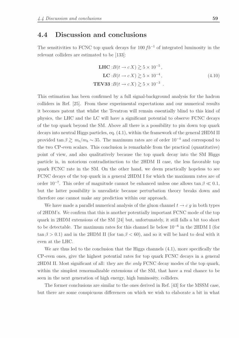
4.4 Discussion and conclusions 59
4.4 Discussion and conclusions
The sensitivities to FCNC top quark decays for 100 fb−1 of integrated luminosity in the
relevant colliders are estimated to be [133]:
LHC :B(t→ cX) & 5× 10⁻⁵ ,
LC :B(t→ cX) & 5× 10⁻⁴ , (4.10)
TEV33 :B(t→ cX) & 5× 10⁻³ .
This estimation has been confirmed by a full signal-background analysis for the hadron
colliders in Ref. [25]. From these experimental expectations and our numerical results
it becomes patent that whilst the Tevatron will remain essentially blind to this kind of
physics, the LHC and the LC will have a significant potential to observe FCNC decays
of the top quark beyond the SM. Above all there is a possibility to pin down top quark
decays into neutral Higgs particles, eq. (4.1), within the framework of the general 2HDM II
provided tanβ & mt/mb ∼ 35. The maximum rates are of order 10−4 and correspond to
the two CP-even scalars. This conclusion is remarkable from the practical (quantitative)
point of view, and also qualitatively because the top quark decay into the SM Higgs
particle is, in notorious contradistinction to the 2HDM II case, the less favorable top
quark FCNC rate in the SM. On the other hand, we deem practically hopeless to see
FCNC decays of the top quark in a general 2HDM I for which the maximum rates are of
order 10−7. This order of magnitude cannot be enhanced unless one allows tan β ≪ 0.1,
but the latter possibility is unrealistic because perturbation theory breaks down and
therefore one cannot make any prediction within our approach.
We have made a parallel numerical analysis of the gluon channel t→ c g in both types
of 2HDM’s. We confirm that this is another potentially important FCNC mode of the top
quark in 2HDM extensions of the SM [24] but, unfortunately, it still falls a bit too short
to be detectable. The maximum rates for this channel lie below 10−6 in the 2HDM I (for
tan β > 0.1) and in the 2HDM II (for tan β < 60), and so it will be hard to deal with it
even at the LHC.
We are thus led to the conclusion that the Higgs channels (4.1), more specifically the
CP-even ones, give the highest potential rates for top quark FCNC decays in a general
2HDM II. Most significant of all: they are the only FCNC decay modes of the top quark,
within the simplest renormalizable extensions of the SM, that have a real chance to be
seen in the next generation of high energy, high luminosity, colliders.
The former conclusions are similar to the ones derived in Ref. [43] for the MSSM case,
but there are some conspicuous differences on which we wish to elaborate a bit in what

60 Loop Induced FCNC Decays of the Top Quark in a General 2HDM
follows [134]. First, in the general 2HDM II the two channels t→ (h0, H0) c give the same
maximum rates, provided we look at different (disjoint) regions of the parameter space.
The t → A0 c channel is, as mentioned, negligible with respect to the CP-even modes.
Hereafter we will discard this FCNC top quark decay mode from our discussions within the
2HDM context. On the other hand, in the MSSM there is a most distinguished channel,
viz. t → h0 c, which can be high-powered by the SUSY stuff all over the parameter
space. In this framework the mixing angle α becomes stuck once tan β and the rest of the
independent parameters are given, and so there is no possibility to reconvert the couplings
between h0 and H0 as in the 2HDM. Still, we must emphasize that in the MSSM the other
two decays t→ H0 c and t→ A0 c can be competitive with t→ h0 c in certain portions
of parameter space. For example, t→ H0 c becomes competitive when the pseudoscalar
mass is in the range 110GeV < mA0 . 170GeV [43]. The possibility of having more
than one FCNC decay (4.1) near the visible level is a feature which is virtually impossible
in the 2HDM II. Second, the reason why t → h0 c in the MSSM is so especial is that it
is the only FCNC top quark decay (4.1) which is always kinematically open throughout
the whole MSSM parameter space, while in the 2HDM all of the decays (4.1) could be,
in the worse possible situation, dead closed. Nevertheless, this is not the most likely
situation in view of the fact that all hints from high precision electroweak data seem to
recommend the existence of (at least) one relatively light Higgs boson [132, 134]. This
is certainly an additional motivation for our work, as it leads us to believe that in all
possible (renormalizable) frameworks beyond the SM, and not only in SUSY, we should
expect that at least one FCNC decay channel (4.1) could be accessible. Third, the main
origin of the maximum FCNC rates in the MSSM traces back to the tree-level FCNC
couplings of the gluino [43]. These are strong couplings, and moreover they are very
weakly restrained by experiment. In the absence of such gluino couplings, or perhaps by
further experimental constraining of them in the future, the FCNC rates in the MSSM
would boil down to just the electroweak (EW) contributions, to wit, those induced by
charginos, squarks and also from SUSY Higgses. The associated SUSY-EW rate is of
order 10−6 at most, and therefore it is barely visible, most likely hopeless even for the
LHC. In contrast, in the general 2HDM the origin of the contributions is purely EW and
the maximum rates are two orders of magnitude higher than the full SUSY-EW effects in
the MSSM. It means that we could find ourselves in the following situation. Suppose that
the FCNC couplings of the gluino get severely restrained in the future and that we come
to observe a few FCNC decays of the top quark into Higgs bosons, perhaps at the LHC
and/or the LC. Then we would immediately conclude that these Higgs bosons could not
be SUSY-MSSM, whilst they could perhaps be CP-even members of a 2HDM II. Fourth,

4.4 Discussion and conclusions 61
the gluino effects are basically insensitive to tanβ, implying that the maximum MSSM
rates are achieved equally well for low, intermediate or high values of tanβ, whereas the
maximum 2HDM II rates (comparable to the MSSM ones) are attained only for high
tan β.
The last point brings about the following question: what could we possibly conclude if
the gluino FCNC couplings were not further restricted by experiment and the tagging of
certain FCNC decays of the top quark into Higgs bosons would come into effect? Would
still be possibly to discern whether the Higgs bosons are supersymmetric or not? The
answer is, most likely yes, provided certain additional conditions would be met.
There are many possibilities and corresponding strategies, but we will limit ourselves
to point out some of them. For example, let us consider the type of signatures involved in
the tagging of the Higgs channels. In the favorite FCNC region (4.7) of the 2HDM II, the
combined decay t → h c → cbb is possible only for h0 or for H0, but not for both – Cf.
Fig. 4.3a – whereas in the MSSM, h0 together with H0, are highlighted for 110GeV <
mA0 < mt, with no preferred tan β value. And similarly, t→ A0 c is also non-negligible for
mA0 . 120GeV [43]. Then the process t→ h c→ cbb gives rise to high pT charm-quark
jets and a recoiling bb pair with large invariant mass. It follows that if more than one
distinctive signature of this kind would be observed, the origin of the hypothetical Higgs
particles could not probably be traced back to a 2HDM II.
One might worry that in the case of h0 and H0 they could also (in principle) decay
into electroweak gauge boson pairs h0, H0 → VewV ew, which in some cases could be
kinematically possible. But this is not so in practice for the 2HDM II if we stick to
our favorite scenario, eq. (4.7). In fact, we recall that the decay h0 → VewV ew is not
depressed with respect to the SM Higgs boson case provided β − α = π/2, and similarly
for H0 → VewV ew if β − α = 0. However, neither of these situations is really pinpointed
by FCNC physics because we have found β ≃ π/2 in the most favorable region of our
numerical analysis, and moreover α was also seen there to be either α ≃ π/2 (for h0) or 0
(for H0), so both decays h0, H0 → VewV ew are suppressed in the regions where the FCNC
rates of the parent decays t → (h0, H0) c are maximized. Again, at variance with this
situation, in the MSSM case H0 → VewV ew is perfectly possible – not so h0 → VewV ew
due to the aforementioned upper bound on mh0 – because tan β has no preferred value in
the most favorable MSSM decay region of t → H0 c. Therefore, detection of a high pT
charm-quark jet against a VewV ew pair of large invariant mass could only be advantageous
in the MSSM, not in the 2HDM. Similarly, for tanβ & 1 the decay H0 → h0 h0 (with real
or virtual h0) is competitive in the MSSM [135,136] in a region where the parent FCNC
top quark decay is also sizeable. Again this is impossible in the 2HDM II and therefore

62 Loop Induced FCNC Decays of the Top Quark in a General 2HDM
it can be used to distinguish the two (SUSY and non-SUSY) Higgs frames.
Finally, even if we place ourselves in the high tanβ region both for the MSSM and the
2HDM II, then the two frameworks could still possibly be separated provided that two
Higgs masses were known, perhaps one or both of them being determined from the tagged
Higgs decays themselves, eq. (4.1). Suppose that tanβ is numerically known (from other
processes or from some favorable fit to precision data), then the full spectrum of MSSM
Higgs bosons would be approximately determined (at the tree level) by only knowing
one Higgs mass, a fact that could be used to check whether the other measured Higgs
mass becomes correctly predicted. Of course, the radiative corrections to the MSSM
Higgs mass relations can be important at high tanβ [114], but these could be taken into
account from the approximate knowledge of the relevant sparticle masses obtained from
the best fits available to the precision measurements within the MSSM. If there were
significant departures between the predicted mass for the other Higgs and the measured
one, we would probably suspect that the tagged FCNC decays into Higgs bosons should
correspond to a non-supersymmetric 2HDM II.
At the end of the day we see that even though the maximum FCNC rates for the
MSSM and the 2HDM II are both of order 10−4 – and therefore potentially visible – at
some point on the road it should be possible to disentangle the nature of the Higgs model
behind the FCNC decays of the top quark. Needless to say, if all the fuss at CERN [132]
about the possible detection of a Higgs boson would eventually be confirmed, this could
still be interpreted as the discovery of one neutral member of an extended Higgs model.
Obviously the combined Higgs data from LEP 200 and the possible discovery of FCNC
top quark decays into Higgs bosons at the LHC/LC would be an invaluable cross-check
of the purportedly new phenomenology.
We emphasize our most essential conclusions in a nutshell: i) Detection of FCNC top
quark decay channels into a neutral Higgs boson would be a blazing signal of physics
beyond the SM; ii) There is a real chance for seeing rare events of that sort both in
generic Type II 2HDM’s and in the MSSM. The maximum rates for the leading FCNC
processes (4.1) and (4.2) in the 2HDM II (resp. in the MSSM) satisfy the relations
B(t→ g c) < 10−6(10−5) < B(t→ h c) ∼ 10−4 , (4.11)
where it is understood that h is h0 or H0, but not both, in the 2HDM II; whereas h is
most likely h0, but it could also be H0 and A0, in the MSSM ; iii) Detection of more than
one Higgs channel would greatly help to unravel the type of underlying Higgs model.
The pathway to seeing new physics through FCNC decays of the top quark is thus
potentially open. It is now an experimental challenge to accomplish this program using

4.4 Discussion and conclusions 63
the high luminosity super-colliders round the corner.
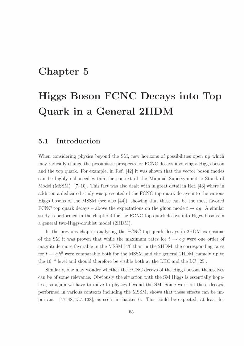
Chapter 5
Higgs Boson FCNC Decays into Top
Quark in a General 2HDM
5.1 Introduction
When considering physics beyond the SM, new horizons of possibilities open up which
may radically change the pessimistic prospects for FCNC decays involving a Higgs boson
and the top quark. For example, in Ref. [42] it was shown that the vector boson modes
can be highly enhanced within the context of the Minimal Supersymmetric Standard
Model (MSSM) [7–10]. This fact was also dealt with in great detail in Ref. [43] where in
addition a dedicated study was presented of the FCNC top quark decays into the various
Higgs bosons of the MSSM (see also [44]), showing that these can be the most favored
FCNC top quark decays – above the expectations on the gluon mode t→ c g. A similar
study is performed in the chapter 4 for the FCNC top quark decays into Higgs bosons in
a general two-Higgs-doublet model (2HDM).
In the previous chapter analysing the FCNC top quark decays in 2HDM extensions
of the SM it was proven that while the maximum rates for t → c g were one order of
magnitude more favorable in the MSSM [43] than in the 2HDM, the corresponding rates
for t → c h0 were comparable both for the MSSM and the general 2HDM, namely up to
the 10−4 level and should therefore be visible both at the LHC and the LC [25].
Similarly, one may wonder whether the FCNC decays of the Higgs bosons themselves
can be of some relevance. Obviously the situation with the SM Higgs is essentially hope-
less, so again we have to move to physics beyond the SM. Some work on these decays,
performed in various contexts including the MSSM, shows that these effects can be im-
portant [47, 48, 137, 138], as seen in chapter 6. This could be expected, at least for
65

66 Higgs Boson FCNC Decays into Top Quark in a General 2HDM
heavy quarks in the MSSM, from the general SUSY study (including both strong and
electroweak supersymmetric effects) of the FCNC vertices h t c (h = h0 , H0 , A0) made
in Ref. [43]. However, other frameworks could perhaps be equally advantageous. Here
we are particularly interested in the FCNC Higgs decay modes into top quark within a
general 2HDM, which have not been studied anywhere in the literature to our knowledge.
It means we restrict to Higgs bosons heavier than mt. From the above considerations,
and most particularly on the basis of the detailed results obtained in the previous chapter
4 one may expect that some of the decays of the Higgs bosons
h→ t c , h→ t c (h = h0 , H0 , A0) (5.1)
in a general 2HDM can be substantially enhanced and perhaps can be pushed up to
the visible level, particularly for h0 which is the lightest CP-even spinless state in these
models [6]. This possibility can be of great relevance on several grounds. On the one hand
the severe degree of suppression of the FCNC Higgs decay in the SM obviously implies
that any experimental sign of Higgs-like FCNC decay (5.1) would be instant evidence
of physics beyond the SM. On the other hand, the presence of an isolated top quark
in the final state, unbalanced by any other heavy particle, is an unmistakable carrier of
the FCNC signature. Finally, the study of the maximum FCNC rates for the top quark
modes (5.1) within the 2HDM, which is the simplest non-trivial extension of the SM,
should serve as a fiducial result from which more complicated extensions of the SM can
be referred to. Therefore, we believe there are founded reasons to perform a thorough
study of the FCNC Higgs decays in minimal extensions of the Higgs sector of the SM and
see whether they can be of any help to discover new physics.
The study is organized as follows. In Section 5.2 we summarize the 2HDM interactions
most relevant for our study and estimate the expected FCNC rates of the Higgs decays
in the SM and the general 2HDM. In Section 5.3 a detailed numerical analysis of the
one-loop calculations of the FCNC decay widths and production rates of FCNC Higgs
events is presented. Finally, in Section 5.4 we discuss the reach of our results and its
phenomenological implications, and deliver our conclusions.
5.2 Expected branching ratios in the SM and the
2HDM
Before presenting the detailed numerical results of our calculation, it may be instructive
to estimate the typical expected widths and branching ratios (B) both for the SM decay

5.2 Expected branching ratios in the SM and the 2HDM 67
HSM → t c and the non-standard decays (5.1) in a general 2HDM. This should be
especially useful in this kind of rare processes, which in the strict context of the SM are
many orders of magnitude out of the accessible range. Therefore, one expects to be able
to grossly reproduce the order of magnitude from simple physical considerations based
on dimensional analysis, power counting, CKM matrix elements and dynamical features.
By the same token it should be possible to guess at the potential enhancement factors in
the 2HDM extension of the SM. In fact, guided by the previous criteria the FCNC decay
width of the SM Higgs of mass mH into top quark is expected to be of order
Γ(HSM → t c) ∼(
1
16π2
)2
|V ∗tbVbc|2 α3
W mH
(
λSMb)4 ∼
( |Vbc|16π2
)2
αW G2F mH m
4b , (5.2)
where GF is Fermi’s constant and αW = g2/4π, g being the SU(2)L weak gauge coupling.
We have approximated the loop form factor by just a constant prefactor. Notice the
presence of λSMb ∼ mb/MW , which is the SM Yukawa coupling of the bottom quark in
units of g. The fourth power of λSMb in (5.2) gives the non-trivial suppression factor rem-
iniscent of the GIM mechanism after summing over flavors. Since we are maximizing our
estimation, a missing function related to kinematics and polarization sums, F (mt/mH) ∼(1−m2
t/m2H)2, has been approximated to one. To obtain the (maximized!) branching ratio
it suffices to divide the previous result by Γ(HSM → b b) ∼ αW(
λSMb)2mH ∼ GF mH m
2b
to obtain
B(HSM → t c) ∼( |Vbc|
16π2
)2
αW GF m2b ∼ 10−13 , (5.3)
with Vbc = 0.04, mb = 5GeV . In general this B will be even smaller, specially for higher
Higgs boson masses (mH > 2MW ) for which the vector boson Higgs decay modes HSM →W+W−(Z Z) can be kinematically available and become dominant. In this case it is easy
to see that B(HSM → t c) will be suppressed by an additional factor of m2b/m
2H , which
amounts at the very least to two additional orders of magnitude suppression, bringing it to
a level of less than 10−15. Already the optimized branching ratio (5.3) will remain invisible
to all foreseeable accelerators in the future! To obtain the corresponding maximized
estimation for the 2HDM we use the couplings from (2.42) and the trilinear couplings 2.1.
Let us now first assume large tan β and restrict to Type II models. From the interaction
Lagrangians above it is clear that we may replace λSMb → λSMb tan β in the previous
formulae for the partial width. Moreover, the leading diagrams in the 2HDM contain the
trilinear Higgs couplings λH+H− h. Therefore, the maximum B associated to the FCNC

68 Higgs Boson FCNC Decays into Top Quark in a General 2HDM
decays (5.1) in a general 2HDM II should be of order1
BII(h→ t c) ∼( |Vbc|
16π2
)2
αW GF m2b tan2 β λ2
H+H− h , (5.4)
where λH+H− h is defined here in units of g and dimensionless as compared to Table 2.1.
Clearly a big enhancement factor tan2 β appears, but this does not suffice. Fortunately,
the trilinear couplings λH+H− h for h = h0, H0 (but not for h = A0) carry two additional
sources of potential enhancement (Cf. Table 2.1) which are absent in the MSSM case.
Take e.g. h0, then we see that under appropriate conditions (for example, large tanα and
large tan β) the trilinear coupling behaves as λH+H− h0 ∼ (m2h0 −m2
A0) tan β/(MW mH±),
and in this case
BII(h0 → t c) ∼( |Vbc|
16π2
)2
αW GF m2b tan4 β
(
m2A0 −m2
h0
MW mH±
)2
. (5.5)
So finally BII(h0 → t c), and of course BII(h0 → t c), can be augmented by a huge factor
tan4 β times the square of the relative splitting among the CP-even Higgs decaying boson
mass and the CP-odd Higgs mass. Since the neutral Higgs bosons do not participate in
the loop form factors (see 4.1), it is clear that various scenarios can be envisaged where
these mass splittings can be relevant. In the next section this behaviour will be borne out
by explicit calculations showing that h0 → t c can be raised to the visible level in the case
of the Type II model. As for the Type I model the Higgs trilinear coupling enhancement
is the same, but in the charged Higgs Yukawa coupling all quarks go with a factor cot β;
hence when considering the leading terms in the loops that contribute one sees that in
the corresponding expression (5.4) the term m2b tan2 β is traded for mtmc cot2 β, which
is negligible at high tan β. Both sources of enhancement are needed, and this feature is
only tenable in the 2HDM II. Of course one could resort to the range tan β ≪ 1 for the
Type I models, but this is not theoretically appealing. For example, for tanβ . 0.1 the
top quark Yukawa coupling gt = g mt/(√
2MW sin β), which is present in the interaction
Lagrangians above, is pushed into the non-perturbative region g2t /16π2 & 1 and then
our calculation would not be justified. And what is worse: for the 2HDM I we would
actually need tanβ ≤ O(10−2) to get significant FCNC rates! In short, we consider that
BI(h → t c + t c) is essentially small (for all h), and that these decays remain always
invisible to speak of. Hereafter we abandon the study of the decays (5.1) for the 2HDM
I and restrict ourselves to the general 2HDM II.
1Here we have normalized the B with respect to the h → bb channel only, because the gauge boson
modes will be suppressed in the relevant FCNC region, Cf. Section 3.

5.3 Numerical analysis 69
5.3 Numerical analysis
Let us now substantiate the previous claims and provide the precise numerical results of
the full one-loop calculation of BII(h→ t c+ t c) 2 as well as of the LHC production rates
of these FCNC events. We refer the reader to previous chapters for more details. The
diagrams for the decays (5.1) are shown in Fig. 5.1, and the diagrams for the productions
can be seen in Fig. 5.2. In what follows we present the final results of our numerical
analysis together with a detailed discussion, interpretation and phenomenological appli-
cation. We have performed the calculations with the help of the numeric and algebraic
programs FeynArts, FormCalc and LoopTools [128–130]. The calculation must obviously
be finite without renormalization, and indeed the cancellation of UV divergences in the
total amplitudes was verified explicitly.
The input set for our numerical analysis is given by the data row
(mh0 , mH0, mA0 , mH±, tanα, tanβ) (5.6)
made out of six independent parameters in the general 2HDM. Remaining inputs as
in [75]. In practice there are some phenomenological restrictions on the data (5.6) which
were already described in the chapter 2, particularly [79]. Again, a key parameter is
tan β, with the restriction (2.43). In practice, since Type I models are not considered, the
effective range for our calculation will be the high tanβ end of (2.43).
With these restrictions in mind we have computed the number of FCNC Higgs decay
events into top quark at the LHC:
pp→ h+X → t c (t c) +X (h = h0, H0, A0) . (5.7)
The necessary cross-sections to compute the production of neutral Higgs bosons at this
collider, including all known QCD corrections, have been computed by adapting the codes
HIGLU 1.0 and HQQ 1.0 [139] – originally written for the MSSM case [140]– to the general
case of the 2HDM3. Folding the cross-sections with the one-loop branching ratios of the
processes (5.1) we have obtained the number of FCNC Higgs decay events at the LHC. Let
us first consider the branching ratios themselves. In Fig. 5.3a,b we show BII(h0 → t c+t c)
for the lightest CP-even state. In particular, Fig. 5.3a shows BII(h0 → t c + t c) versus
the charged Higgs mass mH± . In this figure we fix the values of the parameters in (5.6)
2Here and throughout we use the notation BII(h0 → t c + t c) ≡ BII(h0 → t c) + BII(h0 → t c).3We have used the default parton distribution functions and renormalization/factorization scales used
in these programs, namely GRV94 with µR = µF = mh for HIGLU, and CTEQ4L with µR = µF =√
s ≡√
(ph + pQ + pQ)2 for HQQ.
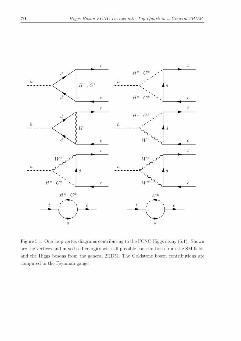
70 Higgs Boson FCNC Decays into Top Quark in a General 2HDM
h
c
d
t
H± , G±
d
h
c
H± , G±
t
d
H± , G±
h
c
d
t
W±
d
h
c
H± , G±
t
d
W±
h
c
W±
t
d
H± , G±
h
c
W±
t
d
W±
t
d
H± , G±
c t
d
W±
c
Figure 5.1: One-loop vertex diagrams contributing to the FCNC Higgs decay (5.1). Shown
are the vertices and mixed self-energies with all possible contributions from the SM fields
and the Higgs bosons from the general 2HDM. The Goldstone boson contributions are
computed in the Feynman gauge.

5.3 Numerical analysis 71
g
g
ht , b
t , b
t , bg
t , b
g t , b
t , b
h
t , b
Figure 5.2: Leading order Feynman diagrams for the Higgs boson production at the LHC
100 200 300 400 500 60010
−7
10−6
10−5
10−4
10−3
10−2
200 300 400 50010
−6
10−5
10−4
200 300 400 50010
−1
100
101
102
103
200 300 400 50010
−5
10−4
10−3
10−2
mH± [GeV ]
mh0 [GeV ]mh0 [GeV ]
mh0 [GeV ]
(a) (b)
(c) (d)
gg → h0
qq, gg → h0 + QQ
Figure 5.3: (a)BII(h0 → t c+ t c) versus mH±; (b) Idem, versus mh0 ; (c) The production
cross-section (in pb) of h0 at the LHC versus its mass; (d) δρ2HDM versus mh0, see the
text. In these figures, when a parameter is not varied it is fixed as in eq.(5.8).
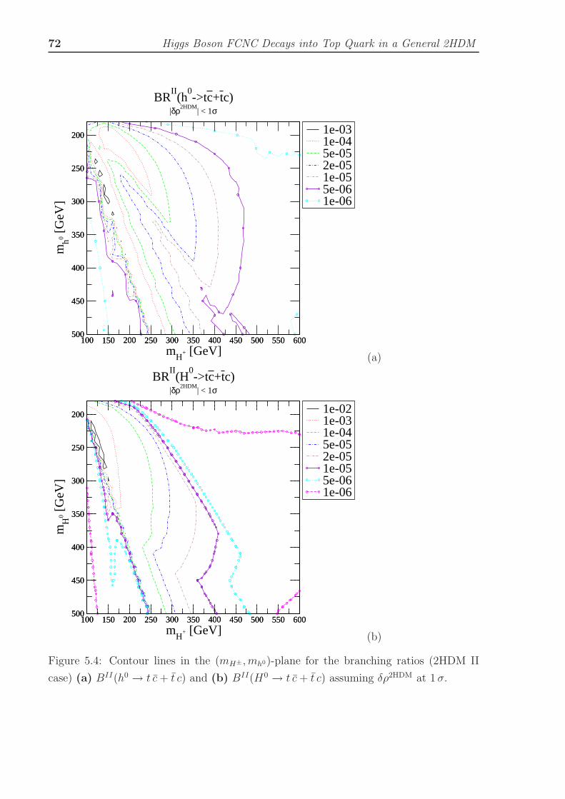
72 Higgs Boson FCNC Decays into Top Quark in a General 2HDM
100 150 200 250 300 350 400 450 500 550 600
200
250
300
350
400
450
500100 150 200 250 300 350 400 450 500 550 600
mH
+ [GeV]
200
250
300
350
400
450
500
mh0 [
GeV
]
1e-031e-045e-052e-051e-055e-061e-06
BRII(h
0->tc+tc)
|δρ2HDM| < 1σ
(a)
100 150 200 250 300 350 400 450 500 550 600
200
250
300
350
400
450
500100 150 200 250 300 350 400 450 500 550 600
mH
+ [GeV]
200
250
300
350
400
450
500
mH
0 [G
eV]
1e-021e-031e-045e-052e-051e-055e-061e-06
BRII(H
0->tc+tc)
|δρ2HDM| < 1σ
(b)
Figure 5.4: Contour lines in the (mH±, mh0)-plane for the branching ratios (2HDM II
case) (a) BII(h0 → t c+ t c) and (b) BII(H0 → t c+ t c) assuming δρ2HDM at 1 σ.

5.3 Numerical analysis 73
100 150 200 250 300 350 400 450 500 550 600
200
250
300
350
400
450
500100 150 200 250 300 350 400 450 500 550 600
mH
+ [GeV]
200
250
300
350
400
450
500
mh0 [
GeV
]500300200150100603020105
Number of events|δρ2HDM
| < 1σ
(a)
100 150 200 250 300 350 400 450 500 550 600
200
250
300
350
400
450
500100 150 200 250 300 350 400 450 500 550 600
mH
+ [GeV]
200
250
300
350
400
450
500
mh0 [
GeV
]
600550500400300250200150
mA
0 [GeV]|δρ2HDM
| < 1σ
(b)
Figure 5.5: (a) Contour lines in the (mH±, mh0)-plane for the maximum number of light
CP-even Higgs FCNC events h0 → t c + t c produced at the LHC for 100 fb−1 of inte-
grated luminosity within δρ2HDM at 1 σ; (b) Contour lines showing the value of mA0 that
maximizes the number of events.
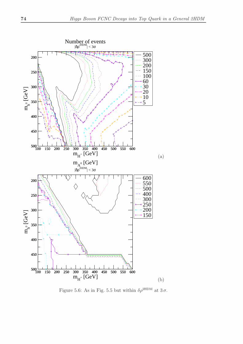
74 Higgs Boson FCNC Decays into Top Quark in a General 2HDM
100 150 200 250 300 350 400 450 500 550 600
200
250
300
350
400
450
500100 150 200 250 300 350 400 450 500 550 600
mH
+ [GeV]
200
250
300
350
400
450
500
mh0 [
GeV
]
500300200150100603020105
Number of events|δρ2HDM
| < 3σ
(a)
100 150 200 250 300 350 400 450 500 550 600
200
250
300
350
400
450
500100 150 200 250 300 350 400 450 500 550 600
mH
+ [GeV]
200
250
300
350
400
450
500
mh0 [
GeV
]
600550500400300250200150
mA
0 [GeV]|δρ2HDM
| < 3σ
(b)
Figure 5.6: As in Fig. 5.5 but within δρ2HDM at 3 σ.

5.3 Numerical analysis 75
100 150 200 250 300 350 400 450 500 550 600
200
250
300
350
400
450
500100 150 200 250 300 350 400 450 500 550 600
mH
+ [GeV]
200
250
300
350
400
450
500
mh0 [
GeV
]
0.40.30.20.10-0.1-0.2-0.3-0.4
α/π|δρ2HDM
| < 1σ
(a)
100 150 200 250 300 350 400 450 500 550 600
200
250
300
350
400
450
500100 150 200 250 300 350 400 450 500 550 600
mH
+ [GeV]
200
250
300
350
400
450
500
mh0 [
GeV
]
0.40.30.20.10-0.1-0.2-0.3-0.4
α/π|δρ2HDM
| < 3σ
(b)
Figure 5.7: Contour lines α/π = const. (α is the mixing angle in the CP-even sector)
corresponding to Figs. 5.5-5.6 for δρ2HDM at (a) 1 σ and (b) 3 σ .
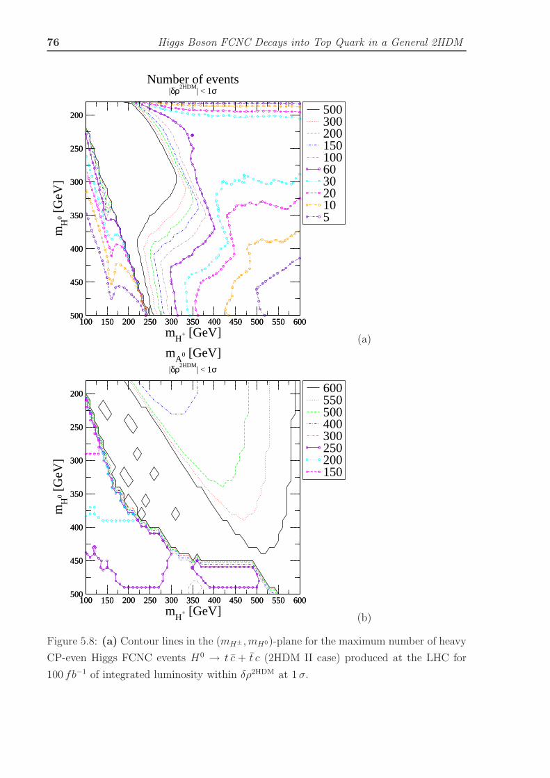
76 Higgs Boson FCNC Decays into Top Quark in a General 2HDM
100 150 200 250 300 350 400 450 500 550 600
200
250
300
350
400
450
500100 150 200 250 300 350 400 450 500 550 600
mH
+ [GeV]
200
250
300
350
400
450
500
mH
0 [G
eV]
500300200150100603020105
Number of events|δρ2HDM
| < 1σ
(a)
100 150 200 250 300 350 400 450 500 550 600
200
250
300
350
400
450
500100 150 200 250 300 350 400 450 500 550 600
mH
+ [GeV]
200
250
300
350
400
450
500
mH
0 [G
eV]
600550500400300250200150
mA
0 [GeV]|δρ2HDM
| < 1σ
(b)
Figure 5.8: (a) Contour lines in the (mH± , mH0)-plane for the maximum number of heavy
CP-even Higgs FCNC events H0 → t c + t c (2HDM II case) produced at the LHC for
100 fb−1 of integrated luminosity within δρ2HDM at 1 σ.

5.3 Numerical analysis 77
100 150 200 250 300 350 400 450 500 550 600
200
250
300
350
400
450
500100 150 200 250 300 350 400 450 500 550 600
mH
+ [GeV]
200
250
300
350
400
450
500
mH
0 [G
eV]
500300200150100603020105
Number of events|δρ2HDM
| < 3σ
(a)
100 150 200 250 300 350 400 450 500 550 600
200
250
300
350
400
450
500100 150 200 250 300 350 400 450 500 550 600
mH
+ [GeV]
200
250
300
350
400
450
500
mH
0 [G
eV]
600550500400300250200150
mA
0 [GeV]|δρ2HDM
| < 3σ
(b)
Figure 5.9: As in Fig. 5.8 but within δρ2HDM at 3 σ.
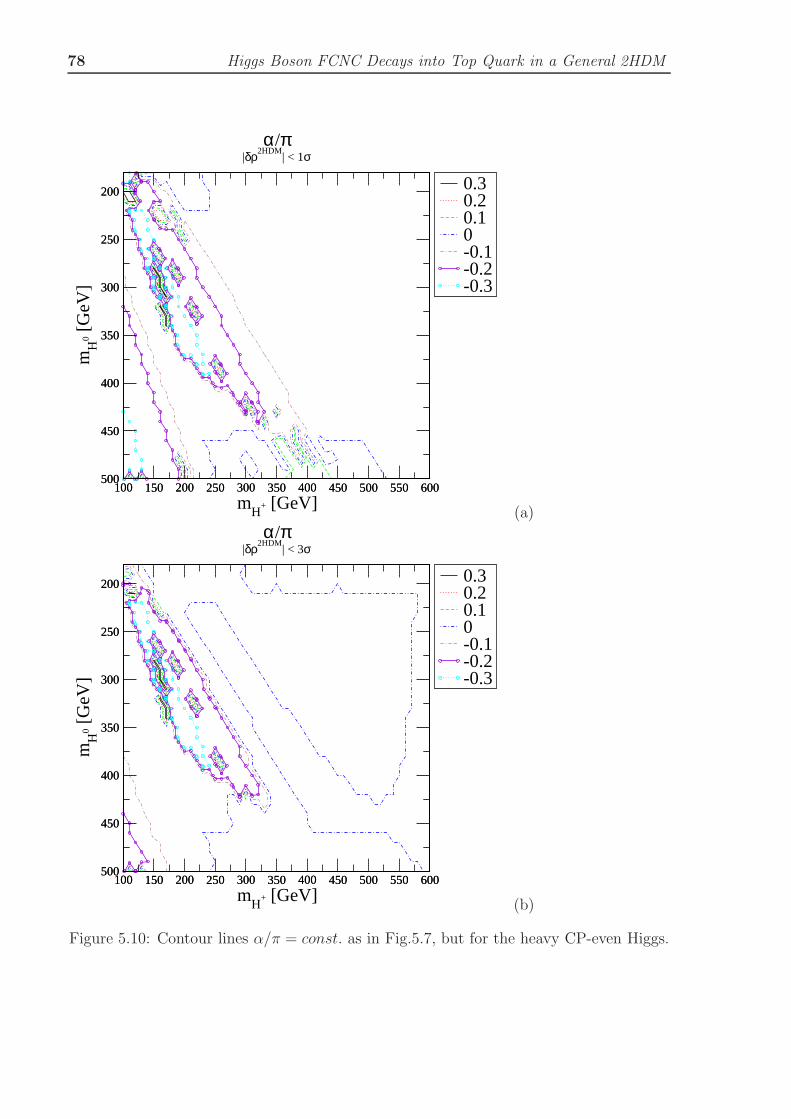
78 Higgs Boson FCNC Decays into Top Quark in a General 2HDM
100 150 200 250 300 350 400 450 500 550 600
200
250
300
350
400
450
500100 150 200 250 300 350 400 450 500 550 600
mH
+ [GeV]
200
250
300
350
400
450
500
mH
0 [G
eV]
0.30.20.10-0.1-0.2-0.3
α/π|δρ2HDM
| < 1σ
(a)
100 150 200 250 300 350 400 450 500 550 600
200
250
300
350
400
450
500100 150 200 250 300 350 400 450 500 550 600
mH
+ [GeV]
200
250
300
350
400
450
500
mH
0 [G
eV]
0.30.20.10-0.1-0.2-0.3
α/π|δρ2HDM
| < 3σ
(b)
Figure 5.10: Contour lines α/π = const. as in Fig.5.7, but for the heavy CP-even Higgs.

5.3 Numerical analysis 79
which are not varying as follows:
(mh0 = 350GeV,mH0 = 600GeV,mA0 = 550GeV,mH± = 375GeV,
tanα = 30, tanβ = 60)(5.8)
After crossing a local maximum (associated to a pseudo-threshold of the one-loop vertex
function involving the h0 H+H− coupling) the subsequently falling behavior of the B with
mH± clearly shows that the previously discussed bounds on mH± are quite relevant. The
branching ratio, however, stays within 10−6−10−5 for a wide range of heavy charged Higgs
masses extending up to mH± ≤ 600GeV in Fig. 5.3a. Hence, for mH± heavy enough to
satisfy the indirect bounds from radiative B-meson decays [62], the maximum B is still
sizeable. In Fig. 5.3c the production rate of h0 bosons at the LHC is shown as a function
of mh0 , for fixed parameters (5.6). The production cross-sections for the subprocesses
gg → h0 +X , gg, qq→ h0 +QQ , (5.9)
contributing to (5.7) in the case of the light CP-even Higgs h0 are explicitly separated in
Fig. 5.3c. The gluon-gluon fusion process proceeds at one-loop and the h0QQ associated
production proceeds at tree-level [136,141]. Similar subprocesses and results apply for H0
and A0 production. At large tanβ and the larger the Higgs boson masses the particular
associated production mechanism with the bottom quark, Q = b, i.e. h0 bb, becomes
dominant by far. All other mechanisms for Higgs boson production in Type II models
[31, 136, 140, 141], like vector-boson fusion (which contributes also to h0QQ when Q are
light quarks), vector-boson bremsstrahlung (qq → hV ) and associated t t production, are
subdominant at large tanβ and can be neglected for our purposes. Admittedly, some of
these mechanisms can be relevant for Higgs boson production in the case of the Type I
2HDM at low tan β, but we have already warned that the corresponding FCNC branching
ratios are never sufficiently high.
The control over δρ2HDM is displayed in Fig. 5.3d. Recall that δρ is not sensitive
to the mass splitting between mh0 and mH0 , because of CP -conservation in the gauge
boson sector, but it does feel all the other mass splittings among Higgs bosons, charged
and neutral. A more systematic search of B values in the parameter space is presented in
Figs. 5.4a,b corresponding to BII(h0 → t c+t c) and BII(H0 → t c+t c) respectively. Here
we have scanned independently on the parameters (5.6) while holding the δρ2HDM bound
at 1 σ. The contour lines in these figures represent the locus of points in the (mH± , mh0)-
plane giving maximized values of the B in the 2HDM II. Let us remark that the highest
value of tanβ is always preferred, and therefore all these contour lines correspond to
tan β = 60.

80 Higgs Boson FCNC Decays into Top Quark in a General 2HDM
In practice, to better assess the possibility of detection at the LHC, one has to study the
production rates of the FCNC events. These are determined by combining the production
cross-sections of neutral 2HDM II Higgs bosons at the LHC and the FCNC branching
ratios. If we just adopt the mild LEP bound mH± & 80GeV and let mH± approach the
maximum in Fig. 5.3a then the B can be as large as 10−3 and the number of FCNC
events can be huge, at the level of ten thousand per 100 fb−1 of integrated luminosity.
But of course the region near the maximum is too special. Moreover, if we switch on the
above mentioned indirect bound from b → s γ [62], then the typical B is much smaller
(of order 10−5) and the number of events is reduced dramatically, at a level of hundred
or less for the same integrated luminosity. On the other hand it may well happen that
there are regions of parameter space where B ∼ 10−5 (see Fig. 5.4) but the production
cross-section is too small because the decaying Higgs boson is too heavy. Therefore, it is
the product of the two quantities that matters.
The systematic search of the regions of parameter space with the maximum number of
FCNC events for the light CP-even Higgs is presented in the form of contour lines in the
multiple Figs. 5.5 and 5.6. For instance, each isoline in Figs. 5.5a and 5.6a corresponds to
a fixed number of produced FCNC events at the LHC while keeping the value of δρ2HDM
within 1 σ or 3 σ respectively of its central experimental value. When scanning over the
parameter space (5.6) we have found again that tanβ is preferred at the highest allowed
value (tan β = 60) – for Type II models. We have also determined (see Figs. 5.5 b and
5.6 d) the corresponding contour lines for mA0 associated to these events. The mA0-lines
are important because the FCNC processes under consideration are sensitive to the mass
splittings between mA0 and the corresponding decaying Higgs boson, see e.g. eq.(5.5)
and Table 2.1. The combined figures 5.5 and 5.6 are very useful because they give a
panoramic view of the origin of our results in the parameter space. To complete the map
of the numerical analysis we provide Fig. 5.7 in which we have projected the contour lines
of the CP-even mixing angle α associated to the previous plots. For a given contour line
α/π = const., the set of inner points have a value of α/π smaller than the one defined
by the line itself. In particular, the large domains in Figs. 5.7a,b without contour lines
correspond to α/π > 0.4 and so to relatively large (and positive) tanα. There are a few
and small neighborhoods where the FCNC rates for h0 can be sizeable also for small tanα.
Knowing that high tanα is generally preferred by h0 → t c + t c, and noting from
Figs. 5.5 and 5.6 that large mass splittings between mh0 and mA0 are allowed, we find that
the trilinear coupling λH+H− h0 can take the form λH+H− h0 ∼ (m2h0−m2
A0) tan β/(MW mH±).
Hence it provides a substantial additional enhancement beyond the tan β factor. One can
check from the approximate formula (5.5) that the maximum FCNC branching ratios

5.3 Numerical analysis 81
BII(h0 → t c+ t c) can eventually reach the 10−5 level even in regions where the charged
Higgs boson mass preserve the stringent indirect bounds from radiative B-meson de-
cays [62]. These expectations are well in agreement with the exact numerical analysis
presented in Fig. 5.4, thus showing that eq.(5.5) provides a reasonable estimate, and there-
fore a plausible explanation for the origin of the maximum contributions. As a matter of
fact, we have checked that the single (finite) Feynman diagram giving rise to the estima-
tion (5.5) – the one-loop vertex Feynman diagram with a couple of charged Higgs bosons
and a bottom quark in the loop – reproduces the full result with an accuracy better than
10% for tanβ & 10−20. At lower tan β values large deviations are possible but, as warned
before, eq. (5.5) is expected to be valid only at large tanβ. Furthermore, for low values
of tanβ . 20 the FCNC Bs are too small to be of any phenomenological interest. The
exact numerical analysis is of course based on the full expression for the branching ratio
BII(h0 → t c+ t c) =Γ(h0 → t c+ t c)
Γ(h0 → b b) + Γ(h0 → t t) + Γ(h0 → V V ) + Γ(h0 → HH), (5.10)
where all decay widths in the denominator of this formula have been computed at the
tree-level in the 2HDM II, since this provides a consistent description of eq. (5.10) at
leading order. Here we have defined
Γ(h0 → V V ) ≡ Γ(h0 →W+W−) + Γ(H0 → Z Z) , (5.11)
Γ(h0 → H H) ≡ Γ(h0 → A0A0) + Γ(h0 → H+H−) . (5.12)
We disregard the loop induced decay channels, since they have branching ratios below the
percent level all over the parameter space. The τ -lepton decay channel is also neglected,
since it is suppressed by a factor ofO(10−2) with respect the bb-channel in the whole 2HDM
parameter space. In general the effect of the gauge boson channels h0 → W+W−, ZZ
in the B (5.10) is not so important as in the SM, actually for β = α they vanish in the
h0 case because they are proportional to sin2(β − α). This is approximately the case
for large tanα and large tan β, the dominant FCNC region for h0 decay (Cf. Fig.5.7a
and 5.7b). In this region, the mode h0 → t t is, when kinematically allowed, suppressed:
B(h0 → t t) ∝ cos2 α/ sin2 β → 0 (Cf. Eq. (2.42)). On the other hand there are domains in
our plots where the decays h0 → H+H− and h0 → A0A0 are kinematically possible and
non-(dynamically) suppressed. Indeed, this can be checked from the explicit structure
of the trilinear couplings h0H+H− and h0A0A0 in Table 2.1; in the dominant region
for the decays h0 → t c + t c both of these couplings are tanβ-enhanced. Nevertheless
the decay h0 → A0A0 is only possible for mA0 < mh0/2 , and since the optimal FCNC
regions demand the largest possible values of mA0 , this decay is kinematically blocked
82 Higgs Boson FCNC Decays into Top Quark in a General 2HDM
there. On the other hand the mode h0 → H+H− is of course allowed if we just take the
aforementioned direct limits on the 2HDM Higgs boson masses. But it is never available
if we apply the indirect bound from b→ s γ on the charged Higgs mass mentioned above,
unless mh0 > 2mH± > 700GeV , in which case h0 is so heavy that its production cross-
section is too small for FCNC studies to be further pursued.
The corresponding results for the heavy CP-even Higgs boson are displayed in Figs.
5.8, 5.9 and 5.10. The exact formula for the B in this case reads
BII(H0 → t c+ t c) =Γ(H0 → t c+ t c)
Γ(H0 → b b) + Γ(H0 → t t) + Γ(H0 → V V ) + Γ(H0 → HH),
(5.13)
where we have defined
Γ(H0 → V V ) ≡ Γ(H0 →W+W−) + Γ(H0 → Z Z) , (5.14)
Γ(H0 → H H) ≡ Γ(H0 → h0 h0) + Γ(H0 → A0A0) + Γ(H0 → H+H−) . (5.15)
From the contour lines in Figs. 5.8a and 5.9a it is patent that the number of FCNC top
quark events stemming from H0 decays is comparable to the case of the lightest Higgs
boson. However, Fig. 5.10a,b clearly reveals that these events are localized in regions of
the parameter space generally different from the h0 case, namely they prefer tanα ≃ 0.
Even so, there are some “islands” of events at large tanα. This situation is complementary
to the one observed for h0 in Fig. 5.7. However, in both cases these isolated regions are
mainly concentrated in the segment mH± < 350GeV . Therefore, if the bound on mH±
from b → s γ is strictly preserved, it is difficult to find regions of parameter space where
the two CP-even states of a general 2HDM II may both undergo a FCNC decay of the
type (5.1).
In the dominant regions of the FCNC mode H0 → t c (where tanα is small and
tanβ is large), the decay of H0 into the tt final state is suppressed: B(H → t t) ∝sin2 α/ sin2 β → 0. In the same regions the gauge boson channels in (5.13) are suppressed
too because Γ(H0 → W+W−, ZZ) ∝ cos2(β − α). In principle the heavy CP-even Higgs
boson H0 also could (as h0) decay into A0A0 and H+H−. But there is a novelty here
with respect to the h0 decays, in that there could be regions where H0 could decay into
the final state h0 h0. This contingency has been included explicitly in eq.(5.15). However,
in practice, neither one of these three last channels is relevant in the optimal FCNC
domains of parameter space. First, the decay H0 → h0 h0, although it is kinematically
possible, is dynamically suppressed in the main FCNC region for H0. This can be seen
from Table 2.1, where the trilinear coupling H0 h0 h0 becomes vanishingly small at large
tanβ and small tanα. Second, the coupling H0A0A0 in Table 2.1 is non-suppressed in

5.3 Numerical analysis 83
the present region, but again the mode H0 → A0 A0 is kinematically forbidden in the
optimal FCNC domains because the latter favor large values of the CP-odd mass (see
Figs. 5.8b and 5.9b). Third, although in these domains the decay H0 → H+H− is also
non-dynamically suppressed (see the corresponding trilinear coupling in Table 2.1), it
becomes kinematically shifted to the high mass range mH0 > 700GeV if we switch on the
indirect bound from b→ s γ. Obviously, in this latter case the H0 production cross section
becomes too small and the FCNC study has no interest. All in all the contributions from
(5.11),(5.12),(5.14) and (5.15) are irrelevant for mh0, mH0 < 700GeV as their numerical
impact on BII(h0, H0 → t c+ t c) is negligible. Our formulae (5.10) and (5.13) do contain
all the decay channels and we have verified explicitly these features.
As remarked before, in general the most favorable regions of parameter space for the
FCNC decays of h0 and H0 do not overlap much. The trilinear Higgs boson self-couplings
in Table 2.1 (also the fermionic ones) are interchanged when performing the simultaneous
substitutions α → π/2 − α and mh0 → mH0 (see last chapter 4). Furthermore, the
LHC production rates of the neutral Higgs bosons fall quite fast with the masses of these
particles, as seen e.g. in Fig. 5.3b for the h0 state. As a consequence that exchange
symmetry on the branching ratios does not go over to the final event rates, so in practice
the number of FCNC events from H0 decays are smaller (for the same values of the other
parameters) as compared to those for h0; thus H0 requires e.g. lighter charged Higgs
masses to achieve the same number of FCNC events as h0. As for the CP-odd state
A0, we have seen that it plays an important indirect dynamical role on the other decays
through the trilinear couplings in Table 2.1, but its own FCNC decay rates never get a
sufficient degree of enhancement due to the absence of the relevant trilinear couplings, so
we may discard it from our analysis.
We notice that this picture is consistent with the decoupling limit in the 2HDM:
for α → β, the heaviest CP-even Higgs boson (H0) behaves as the SM Higgs boson,
whereas h0 decouples from the electroweak gauge bosons and may develop enhanced
couplings to up and down-like quarks, depending on whether tanβ is small or large
respectively; in the opposite limit (α→ β−π/2), it is h0 that behaves as HSM , while H0
decouples from gauge bosons and may develop the same enhanced couplings to quarks
as h0 did in the previous case. Indeed these are the situations that we find concerning
the FCNC decay rates. We recall that the numerical results presented in our figures
correspond to an integrated luminosity of 100 fb−1. However, the combined ATLAS and
CMS detectors might eventually accumulate a few hundred inverse femtobarn [13, 14].
Therefore, hopefully, a few hundred FCNC events (5.1) could eventually be collected in
the most optimistic scenario. Actually, the extreme rareness of these events in the SM

84 Higgs Boson FCNC Decays into Top Quark in a General 2HDM
suggests that if only a few of them could be clearly disentangled, it should suffice to claim
physics beyond the SM.
5.4 Discussion and conclusions
Detection strategies at the CERN-LHC collider for the search of the SM Higgs boson,
and also for the three spinless fields of the MSSM Higgs sector, have been described in
great detail in many places of the literature [6, 11, 13, 14, 17, 142, 143], but not so well
for the corresponding charged and neutral Higgs bosons of the general 2HDM. The result
is that the discovery of the SM Higgs boson is guaranteed at the LHC in the whole
presumed range 100GeV . mH . 1 TeV . However, the discovery channels are different
in each kinematical region and sometimes the most obvious ones are rendered useless. For
example, due to the huge irreducible QCD background from b b dijets, the decay mode
HSM → b b is difficult and one has to complement the search with many other channels,
particularly HSM → γ γ [13,14]. We have shown in this work that there are scenarios in
the 2HDM parameter space where alternative decays, like the FCNC modes h0 → t c+ t c
and H0 → t c + t c, can also be useful. For instance, in the h0 case, this situation occurs
when tanβ and tanα are both large and the CP-odd state is much heavier than the
CP-even ones. The potential enhancement is then spectacular and it may reach up to
ten billion times the SM value B(HSM → t c) ∼ 10−15, thereby bringing the maximum
value of the FCNC branching ratio B(h0 → t c) to the level of ∼ 10−5. As a matter of
fact, the enhancement would be much larger were it not because we eventually apply the
severe (indirect) lower bound on the charged Higgs mass from b → s γ [62]. Although
these decays have maximal ratios below B(h → γγ) ∼ 10−3, they should be essentially
free of QCD background 4.
While in the MSSM almost the full (mA0 , tanβ)-parameter space is covered, with
better efficiency at high tan β though, we should insist that within the general 2HDM the
tagging strategies are not so well studied and one would like to have further information
to disentangle the MSSM scenarios from the 2HDM ones. Here again the study of the
FCNC Higgs decays can play a role. Of course the statistics for the FCNC Higgs decays
is poor due to the weakness of the couplings and the large masses of the Higgs bosons
to be produced. However, in the favorable regions, which are generally characterized
by large values of tan β and of tanα, one may collect a few hundred events of the type
4Misidentification of b-quarks as c-quarks in tb production might be a source of background to our
FCNC events. However, to rate the actual impact of that misidentification one would need a dedicated
simulation of the signal versus background, which is beyond the scope of this work.

5.4 Discussion and conclusions 85
(5.1)– mainly from h0 – in the high luminosity phase of the LHC. As we have said, this
is basically due to the enormous enhancement that may undergo the FCNC decay rates,
but also because in the same regions of parameter space where the Bs are enhanced, also
the LHC production rates of the Higgs bosons can be significantly larger (one order of
magnitude) in the 2HDM II as compared to the SM.
Interestingly enough, in many cases one can easily distinguish whether the enhanced
FCNC events (5.1) stem from the dynamics of a general, unrestricted, 2HDM model, or
rather from some supersymmetric mechanisms within the MSSM. This is already obvious
from the fact that the ranges of neutral and charged Higgs boson masses in the 2HDM
case can be totally incompatible with the corresponding ones in the MSSM. But there
are many other ways to discriminate these rare events. For instance, in the 2HDM case
the CP-odd modes A0 → t c+ t c are completely hopeless whereas in the MSSM they can
be enhanced see chapter 7, [43, 47, 48]. Using this information in combination with the
masses of potentially detected Higgs bosons could be extremely useful to pinpoint the
supersymmetric or non-supersymmetric nature of them. We may describe a few specific
strategies. As it was first shown in Ref. [43], the leading SUSY-FCNC effects associated
to the h t c vertices (h = h0 , H0 , A0) come from the FCNC gluino interactions which
are induced by potentially large misalignments of the quark and squark mass matrices
[93,144]. These effects are not particularly sensitive to tanβ and they can be very sizeable
for both high and moderately low values of this parameter. This sole fact can be another
distinguishing feature between FCNC events (5.1) of MSSM or 2HDM origin. If, for
example, a few of these events were observed and at the same time the best MSSM fits to
the electroweak precision data would favor moderate values of tanβ, say in the range 10−20, then it is clear that those events could originate in the FCNC gluino interactions but
in no way within the context of the general 2HDM. In this respect it should be mentioned
that the FCNC gluino couplings became more restricted from the low-energy meson data
[104], and will presumably become further restricted in the near future. The reason being
that the same couplings are related, via SU(2) gauge invariance and CKM rotation, to
those affecting the down-like quark sector, which will most likely become constrained by
the increasingly more precise low-energy meson physics [95,96,104]. In that circumstance
the only source of FCNC Higgs decays in the MSSM will stem purely from the electroweak
interactions within the super-CKM basis. Then, in the absence of these SUSY-QCD
FCNC effects, we could judiciously conclude from the work of Ref. [43] – in which both
the SUSY-QCD and the SUSY electroweak contributions were computed for the h t c
vertices – that the FCNC rates in the MSSM should diminish dramatically (two to three
orders of magnitude). In such case we can imagine the following “provocative” scenario.

86 Higgs Boson FCNC Decays into Top Quark in a General 2HDM
Suppose that the LHC finds a light neutral Higgs boson of mass . 140GeV (suggestively
enough, in a mass range near the MSSM upper bound formh0!) and subsequently, or about
simultaneously, a charged Higgs boson and another neutral Higgs boson both with masses
around 400GeV or more. At this point one could naively suspect that a MSSM picture
out these findings is getting somehow confirmed. If, however, later on a few FCNC events
(5.1) are reported and potentially ascribed to the previously discovered heavy neutral
Higgs boson (presumably H0), then the overall situation could not correspond at all
to the MSSM, while it could be perfectly compatible with the 2HDM II. Alternatively,
suppose that the FCNC gluino couplings were not yet sufficiently restricted, but (still
following the remaining hypotheses of the previous example) a third neutral Higgs boson
(presumably A0) is found, also accompanied with a few FCNC events. Then this situation
would be incompatible with the 2HDM II, and in actual fact it would put forward strong
(indirect) evidence of the MSSM!!
We should also mention that there are other FCNC Higgs decay modes, as for example
h → b s + b s, which could be, in principle, competitive with the top quark modes (5.1).
In some cases these bottom modes can be highly enhanced in the MSSM case [47, 48].
Actually, a more complete assessment of the FCNC bottom modes in the MSSM case is
studied in the chapter 6 – namely one which takes also into account the supersymmet-
ric contributions to the highly restrictive radiative B-meson decays – shows that they
are eventually rendered at a similar level of the top modes under study in most of the
parameter space.
To summarize, the FCNC decays of the Higgs bosons into top quark final states can
be a helpful complementary strategy to search for signals of physics beyond the SM in the
LHC. Our comprehensive numerical analysis shows that the FCNC studies are feasible for
CP-even Higgs masses up to about 500GeV . While the statistics of these FCNC decays
is of course poor, the advantage is that a few tagged and well discriminated events of this
sort could not be attributed by any means to the SM, and therefore should call for various
kinds of new physics. In this work we have shown that a general 2HDM II is potentially
competitive to be ultimately responsible for these FCNC decays, if they are ever found,
and we have exemplified how to discriminate this possibility from the more restricted one
associated to the MSSM.
Chapter 6
Higgs Boson FCNC Decays into
Bottom Quarks in the MSSM
6.1 Introduction
The most general MSSM includes tree-level FCNCs among the extra predicted particles,
which induce one-loop FCNC interactions among the SM particles, as discussed in section
3.6.
Concerning the FCNC interactions of Higgs bosons with third generation quarks, it was
demonstrated long ago [43] that the leading term corresponds to a single particle insertion
approximation, which produces a flavor change in the internal squark loop propagator,
since in this case the chirality change can already take place at the squark-squark-Higgs
boson interaction vertex. Adding this to the fact that the Higgs bosons (in contrast to
gauge bosons) have a privileged coupling to third generation quarks, one might expect
that the FCNC interactions of the type quark-quark-Higgs bosons in the MSSM become
highly strengthened with respect to the SM prediction. This was already proven in the
rare decay channels Γ(t→ ch) [43] (h being any of the neutral Higgs bosons of the MSSM
h ≡ h0, H0, A0), where the maximum rate of the SUSY-QCD induced branching ratio
was found to be B(t→ ch) ≃ 10−5, eight orders of magnitude above the SM expectations
B(t → cHSM) ≃ 10−13. Similar enhancement factors have been found in the top-quark-
Higgs boson interactions in other extensions of the SM, as seen in chapters 4-7.
From the experience of the previous calculations with the top quark, we expect similar
enhancements in the FCNC interactions of the MSSM Higgs bosons with the bottom
quark. Indeed, the purpose of this work is to quantify, in a reliable way, the MSSM
87
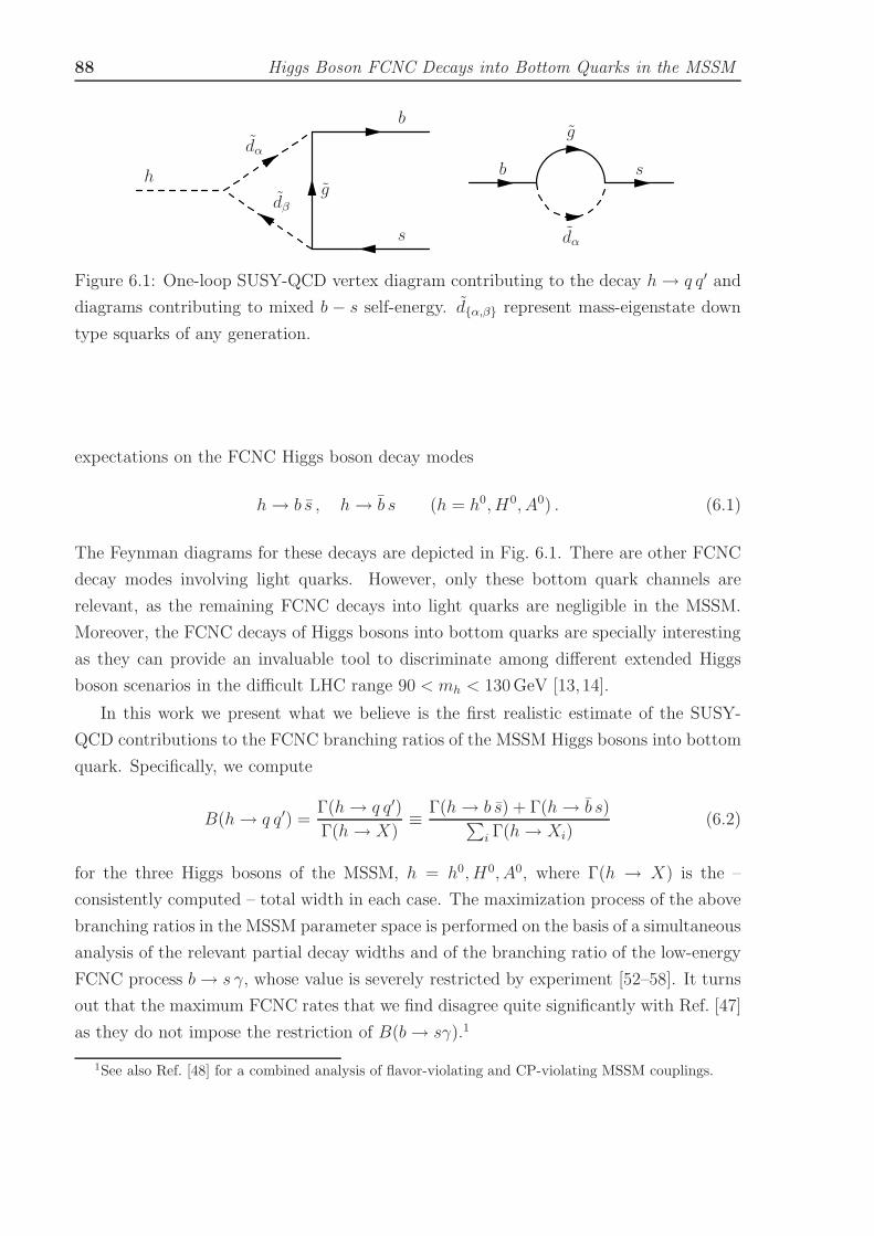
88 Higgs Boson FCNC Decays into Bottom Quarks in the MSSM
h
s
dα
b
gdβ
b
dα
g
s
Figure 6.1: One-loop SUSY-QCD vertex diagram contributing to the decay h→ q q′ and
diagrams contributing to mixed b − s self-energy. d{α,β} represent mass-eigenstate down
type squarks of any generation.
expectations on the FCNC Higgs boson decay modes
h→ b s , h→ b s (h = h0, H0, A0) . (6.1)
The Feynman diagrams for these decays are depicted in Fig. 6.1. There are other FCNC
decay modes involving light quarks. However, only these bottom quark channels are
relevant, as the remaining FCNC decays into light quarks are negligible in the MSSM.
Moreover, the FCNC decays of Higgs bosons into bottom quarks are specially interesting
as they can provide an invaluable tool to discriminate among different extended Higgs
boson scenarios in the difficult LHC range 90 < mh < 130GeV [13,14].
In this work we present what we believe is the first realistic estimate of the SUSY-
QCD contributions to the FCNC branching ratios of the MSSM Higgs bosons into bottom
quark. Specifically, we compute
B(h→ q q′) =Γ(h→ q q′)
Γ(h→ X)≡ Γ(h→ b s) + Γ(h→ b s)
∑
i Γ(h→ Xi)(6.2)
for the three Higgs bosons of the MSSM, h = h0, H0, A0, where Γ(h → X) is the –
consistently computed – total width in each case. The maximization process of the above
branching ratios in the MSSM parameter space is performed on the basis of a simultaneous
analysis of the relevant partial decay widths and of the branching ratio of the low-energy
FCNC process b→ s γ, whose value is severely restricted by experiment [52–58]. It turns
out that the maximum FCNC rates that we find disagree quite significantly with Ref. [47]
as they do not impose the restriction of B(b→ sγ).1
1See also Ref. [48] for a combined analysis of flavor-violating and CP-violating MSSM couplings.

6.2 Partial widths and branching ratios 89
The structure of the study is as follows. In Section 6.2 we estimate the expected
branching ratios and describe the structure of Eq. (6.2) in the MSSM in more detail; in
Section 6.3 we present the numerical analysis, and in Section 6.4 we deliver our conclusions.
6.2 Partial widths and branching ratios
As seen in eqs. (1.5) and (1.6) the branching ratios into bottom quark are much larger
than the Higgs boson FCNC branching ratio into top quark in the SM as seen in chapter
5. However, even in the case (1.5) it is still too small to have a chance for detection in
the LHC. It is clear that unless new physics comes to play the process HSM → b s (and
of course HSM → b s) will remain virtually invisible. Nonetheless the result (1.5) is not
too far from being potentially detectable, and one might hope that it should not be too
difficult for the new physics to boost it up to the observable level.
Consider how to estimate the potentially augmented rates for the MSSM processes
(6.1), if only within a similarly crude approximation as above. Because of the strong
FCNC gluino couplings mentioned in Section 6.1 and the tanβ-enhancement inherent to
the MSSM Yukawa couplings (see Ref. [43] for details), we may expect several orders
of magnitude increase of the branching ratios (6.2) as compared to the previous SM
result. A naive approach might however go too far. For instance, one could look at the
general structure of the couplings and venture an enhancement factor typically of order
(αs/αW )2 tan2 β |δ23/Vts|2, which for δ23 . 1 and tanβ > 30 could easily rocket the SM
result some 5 − 6 orders of magnitude higher, bringing perhaps one of the MSSM rates
(6.2) to the “scandalous” level of 10% or more. But of course only a more elaborated
calculation, assisted by a judicious consideration of the various experimental restrictions,
can provide a reliable result. As we shall see, a thorough analysis generally disproves the
latter overestimate.
The detailed computation of the SUSY-QCD one-loop partial decay widths Γ(h→ q q′)
in (6.2) within the MSSM follows closely that of Γ(t → ch) (see Ref. [43]). The rather
cumbersome analytical expressions will not be listed here as they are an straightforward
adaptation of those presented in the aforementioned references. However, there are a
few subtleties that need to be pointed out. One of them is related to the calculation
of the total widths Γ(h → X) for the three Higgs bosons h = h0, H0, A0 in the MSSM.
As long as Γ(h → q q′) in the numerator of Eq. (6.2) is computed at leading order, the
denominator has to be computed also at leading order, otherwise an artificial enhancement
of B(h→ q q′) can be generated. For example, including the next-to-leading (NLO) order
QCD corrections to Γ(h→ bb) reduces the decay width by a significant amount [145–149].
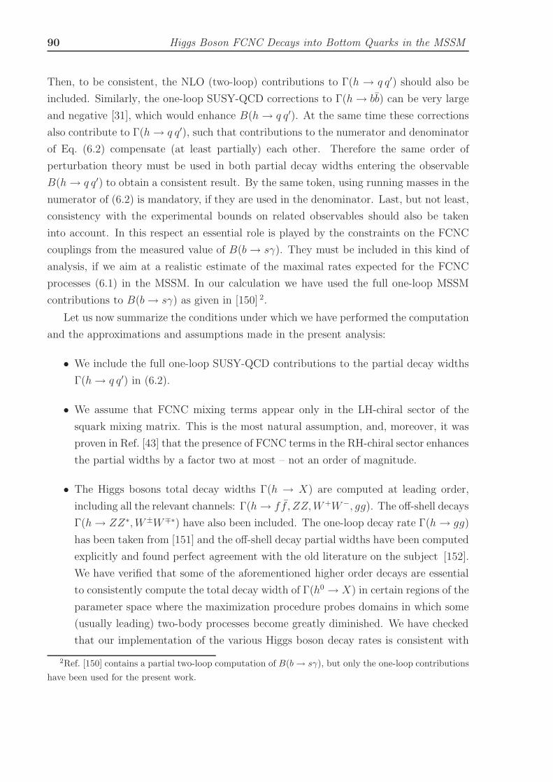
90 Higgs Boson FCNC Decays into Bottom Quarks in the MSSM
Then, to be consistent, the NLO (two-loop) contributions to Γ(h → q q′) should also be
included. Similarly, the one-loop SUSY-QCD corrections to Γ(h→ bb) can be very large
and negative [31], which would enhance B(h→ q q′). At the same time these corrections
also contribute to Γ(h→ q q′), such that contributions to the numerator and denominator
of Eq. (6.2) compensate (at least partially) each other. Therefore the same order of
perturbation theory must be used in both partial decay widths entering the observable
B(h→ q q′) to obtain a consistent result. By the same token, using running masses in the
numerator of (6.2) is mandatory, if they are used in the denominator. Last, but not least,
consistency with the experimental bounds on related observables should also be taken
into account. In this respect an essential role is played by the constraints on the FCNC
couplings from the measured value of B(b→ sγ). They must be included in this kind of
analysis, if we aim at a realistic estimate of the maximal rates expected for the FCNC
processes (6.1) in the MSSM. In our calculation we have used the full one-loop MSSM
contributions to B(b→ sγ) as given in [150] 2.
Let us now summarize the conditions under which we have performed the computation
and the approximations and assumptions made in the present analysis:
• We include the full one-loop SUSY-QCD contributions to the partial decay widths
Γ(h→ q q′) in (6.2).
• We assume that FCNC mixing terms appear only in the LH-chiral sector of the
squark mixing matrix. This is the most natural assumption, and, moreover, it was
proven in Ref. [43] that the presence of FCNC terms in the RH-chiral sector enhances
the partial widths by a factor two at most – not an order of magnitude.
• The Higgs bosons total decay widths Γ(h → X) are computed at leading order,
including all the relevant channels: Γ(h→ f f , ZZ,W+W−, gg). The off-shell decays
Γ(h→ ZZ∗,W±W∓∗) have also been included. The one-loop decay rate Γ(h→ gg)
has been taken from [151] and the off-shell decay partial widths have been computed
explicitly and found perfect agreement with the old literature on the subject [152].
We have verified that some of the aforementioned higher order decays are essential
to consistently compute the total decay width of Γ(h0 → X) in certain regions of the
parameter space where the maximization procedure probes domains in which some
(usually leading) two-body processes become greatly diminished. We have checked
that our implementation of the various Higgs boson decay rates is consistent with
2Ref. [150] contains a partial two-loop computation of B(b→ sγ), but only the one-loop contributions
have been used for the present work.
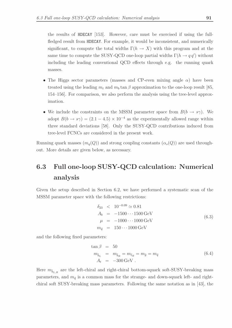
6.3 Full one-loop SUSY-QCD calculation: Numerical analysis 91
the results of HDECAY [153]. However, care must be exercised if using the full-
fledged result from HDECAY. For example, it would be inconsistent, and numerically
significant, to compute the total widths Γ(h → X) with this program and at the
same time to compute the SUSY-QCD one-loop partial widths Γ(h→ q q′) without
including the leading conventional QCD effects through e.g. the running quark
masses.
• The Higgs sector parameters (masses and CP-even mixing angle α) have been
treated using the leading mt and mb tan β approximation to the one-loop result [85,
154–156]. For comparison, we also perform the analysis using the tree-level approx-
imation.
• We include the constraints on the MSSM parameter space from B(b → sγ). We
adopt B(b → sγ) = (2.1 − 4.5)× 10−4 as the experimentally allowed range within
three standard deviations [58]. Only the SUSY-QCD contributions induced from
tree-level FCNCs are considered in the present work.
Running quark masses (mq(Q)) and strong coupling constants (αs(Q)) are used through-
out. More details are given below, as necessary.
6.3 Full one-loop SUSY-QCD calculation: Numerical
analysis
Given the setup described in Section 6.2, we have performed a systematic scan of the
MSSM parameter space with the following restrictions:
δ23 < 10−0.09 ≃ 0.81
Ab = −1500 · · ·1500GeV
µ = −1000 · · ·1000GeV
mq = 150 · · ·1000GeV
(6.3)
and the following fixed parameters:
tan β = 50
mbL= mbR
= mtR = mg = mq
At = −300GeV .
(6.4)
Here mbL,Rare the left-chiral and right-chiral bottom-squark soft-SUSY-breaking mass
parameters, and mq is a common mass for the strange- and down-squark left- and right-
chiral soft SUSY-breaking mass parameters. Following the same notation as in [43], the
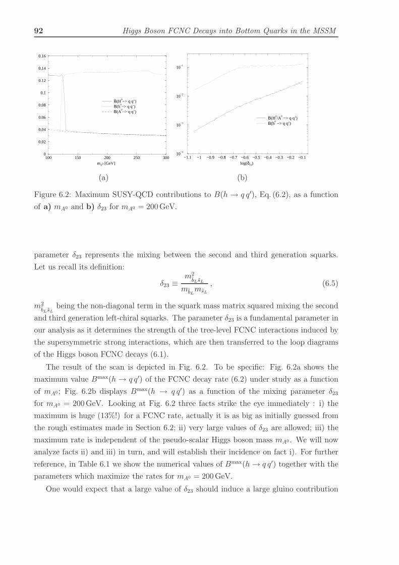
92 Higgs Boson FCNC Decays into Bottom Quarks in the MSSM
100 150 200 250 300mA0 [GeV]
0
0.02
0.04
0.06
0.08
0.1
0.12
0.14
0.16
Β(H0−> q q’)
Β(h0−> q q’)
Β(A0−> q q’)
−1.1 −1 −0.9 −0.8 −0.7 −0.6 −0.5 −0.4 −0.3 −0.2 −0.1log(δ23)
10−4
10−3
10−2
10−1
Β(H0/A
0 −> q q’)
Β(h0 −> q q’)
(a) (b)
Figure 6.2: Maximum SUSY-QCD contributions to B(h → q q′), Eq. (6.2), as a function
of a) mA0 and b) δ23 for mA0 = 200GeV.
parameter δ23 represents the mixing between the second and third generation squarks.
Let us recall its definition:
δ23 ≡m2bLsL
mbLmsL
, (6.5)
m2bLsL
being the non-diagonal term in the squark mass matrix squared mixing the second
and third generation left-chiral squarks. The parameter δ23 is a fundamental parameter in
our analysis as it determines the strength of the tree-level FCNC interactions induced by
the supersymmetric strong interactions, which are then transferred to the loop diagrams
of the Higgs boson FCNC decays (6.1).
The result of the scan is depicted in Fig. 6.2. To be specific: Fig. 6.2a shows the
maximum value Bmax(h→ q q′) of the FCNC decay rate (6.2) under study as a function
of mA0 ; Fig. 6.2b displays Bmax(h → q q′) as a function of the mixing parameter δ23
for mA0 = 200GeV. Looking at Fig. 6.2 three facts strike the eye immediately : i) the
maximum is huge (13%!) for a FCNC rate, actually it is as big as initially guessed from
the rough estimates made in Section 6.2; ii) very large values of δ23 are allowed; iii) the
maximum rate is independent of the pseudo-scalar Higgs boson mass mA0 . We will now
analyze facts ii) and iii) in turn, and will establish their incidence on fact i). For further
reference, in Table 6.1 we show the numerical values of Bmax(h→ q q′) together with the
parameters which maximize the rates for mA0 = 200GeV.
One would expect that a large value of δ23 should induce a large gluino contribution

6.3 Full one-loop SUSY-QCD calculation: Numerical analysis 93
Particle H0 h0 A0
B(h→ q q′) 3.3× 10⁻² 1.3× 10⁻¹ 3.3× 10⁻²
Γ(h→ X) 11.0GeV 1.6× 10⁻³ GeV 11.3GeV
δ23 10−0.09 10−0.1 10−0.09
mq 975GeV 975GeV 975GeV
Ab 1500GeV 730GeV 1290GeV
µ 980GeV 1000GeV 980GeV
B(b→ sγ) 4.42× 10⁻⁴ 4.23× 10⁻⁴ 4.50× 10⁻⁴
Table 6.1: Maximum values of B(h → q q′) and corresponding SUSY parameters for
mA0 = 200GeV.
Particle H0 h0 A0
B(h→ q q′) 9.1× 10⁻⁴ 3.1× 10⁻³ 9.1× 10⁻⁴
Γ(h→ X) 11.2GeV 1.4× 10⁻³ GeV 11.3GeV
δ23 10−0.43 10−0.8 10−0.43
mq 1000GeV 975GeV 1000GeV
Ab −1500GeV −1500GeV −1500GeV
µ −460GeV −1000GeV −460GeV
B(b→ sγ) 4.49× 10⁻⁴ 4.48× 10⁻⁴ 4.49× 10⁻⁴
Table 6.2: Maximum values of B(h → q q′) and corresponding SUSY parameters for
mA0 = 200GeV excluding the window region.
to B(b → sγ). In fact it does! However our automatic scanning process picks up the
corners of parameter space where the gluino contribution alone is much larger than the
SM contribution, but opposite in sign, such that both contributions destroy themselves
partially leaving a result in accordance with the experimental constraints. We exam-
ine this behaviour in Fig. 6.3, where we show the values of B(h → q q′) together with
B(b→ sγ) as a function of δ23 for the parameters which maximize the FCNC rate of the
lightest CP-even state h0 in Table 6.1. We see that, for small values of δ23, the gluino
contribution to B(b → sγ) is small, and the total B(b → sγ) prediction is close to the
SM expectation. In contrast, as δ23 steadily grows, B(b → sγ) decreases fast (mean-
ing a dramatic cancellation between the two contributions) until reaching a point where
B(b → sγ) = 0. From there on it starts to grow with a large slope, and in its race
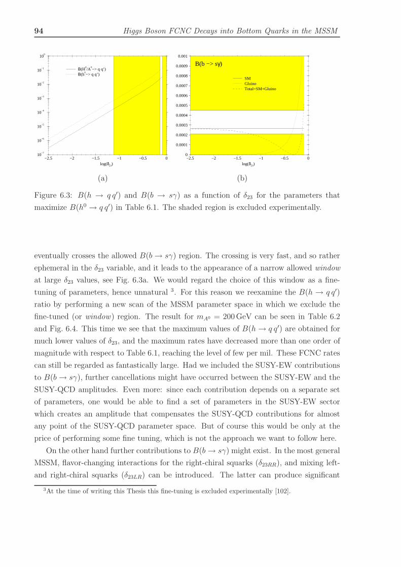
94 Higgs Boson FCNC Decays into Bottom Quarks in the MSSM
−2.5 −2 −1.5 −1 −0.5 0log(δ23)
10−7
10−6
10−5
10−4
10−3
10−2
10−1
100
Β(H0/A
0−> q q’)
Β(h0−> q q’)
−2.5 −2 −1.5 −1 −0.5 0log(δ23)
0
0.0001
0.0002
0.0003
0.0004
0.0005
0.0006
0.0007
0.0008
0.0009
0.001
SMGluinoTotal=SM+Gluino
B(b −> sγ)
(a) (b)
Figure 6.3: B(h → q q′) and B(b → sγ) as a function of δ23 for the parameters that
maximize B(h0 → q q′) in Table 6.1. The shaded region is excluded experimentally.
eventually crosses the allowed B(b→ sγ) region. The crossing is very fast, and so rather
ephemeral in the δ23 variable, and it leads to the appearance of a narrow allowed window
at large δ23 values, see Fig. 6.3a. We would regard the choice of this window as a fine-
tuning of parameters, hence unnatural 3. For this reason we reexamine the B(h → q q′)
ratio by performing a new scan of the MSSM parameter space in which we exclude the
fine-tuned (or window) region. The result for mA0 = 200GeV can be seen in Table 6.2
and Fig. 6.4. This time we see that the maximum values of B(h→ q q′) are obtained for
much lower values of δ23, and the maximum rates have decreased more than one order of
magnitude with respect to Table 6.1, reaching the level of few per mil. These FCNC rates
can still be regarded as fantastically large. Had we included the SUSY-EW contributions
to B(b→ sγ), further cancellations might have occurred between the SUSY-EW and the
SUSY-QCD amplitudes. Even more: since each contribution depends on a separate set
of parameters, one would be able to find a set of parameters in the SUSY-EW sector
which creates an amplitude that compensates the SUSY-QCD contributions for almost
any point of the SUSY-QCD parameter space. But of course this would be only at the
price of performing some fine tuning, which is not the approach we want to follow here.
On the other hand further contributions to B(b→ sγ) might exist. In the most general
MSSM, flavor-changing interactions for the right-chiral squarks (δ23RR), and mixing left-
and right-chiral squarks (δ23LR) can be introduced. The latter can produce significant
3At the time of writing this Thesis this fine-tuning is excluded experimentally [102].

6.3 Full one-loop SUSY-QCD calculation: Numerical analysis 95
100 150 200 250 300mA0
0
0.0005
0.001
0.0015
0.002
0.0025
0.003
0.0035
0.004
Β(H0−> q q’)
Β(h0−> q q’)
Β(A0−> q q’)
−2.0 −1.8 −1.6 −1.4 −1.2 −1.0 −0.8 −0.6 −0.4 −0.2 0.0log(δ23)
10−6
10−5
10−4
10−3
10−2
Β(H0/A
0 −> q q’)
Β(h0 −> q q’)
(a) (b)
Figure 6.4: Maximum value of the SUSY-QCD contributions to B(h→ q q′) as a function
of a) mA0 and b) δ23 for mA0 = 200GeV, for the scenario excluding the window regions.
contributions to B(b → sγ), changing the allowed parameter space. The introduction
of δ23LR can produce two possible outcomes: First, in certain regions of the parameter
space, the contributions of δ23LR and δ23 are of the same sign, enhancing each other. In
this situation, the maximum allowed value of δ23 is obtained for δ23LR = 0. Second, in
other regions of the parameter space the two contributions would compensate each other,
producing an overall value of B(b → sγ) in accordance with experimental constraints,
even though each contribution would be much larger. Again, we would regard these
compensations as unnatural, and would discard that region of the parameter space. In
the following we will require that the SUSY-QCD contributions induced by δ23 do not
compensate the SM ones to give an acceptable value of B(b → sγ); this is equivalent to
the condition that the SUSY-QCD amplitude represents a small contribution to the total
B(b→ sγ) value, and is therefore independent of the inclusion of the other contributions
(SUSY-EW, δ23LR).4
We turn now our view to the second fact, namely the independence of the maximum
rates with respect to mA0 . We will show that it also plays a central role as to the
enhancement of B(h → q q′). Actually, a good hint is given by the small values of the
lightest Higgs boson decay width in Tables 6.1 and 6.2, Γ(h0 → X) ∼ 2 × 10⁻³ GeV.
The maximization process of B(h0 → q q′) does not only find the parameters for which
4The analysis of Ref. [48] follows the opposite approach, that is: to find the fine-tuning conditions
imposed by low energy data that allow for the largest possible value of the FCNC parameters.

96 Higgs Boson FCNC Decays into Bottom Quarks in the MSSM
−1500 −1000 −500 0 500 1000 1500µ [GeV]
10−5
10−4
10−3
10−2
10−1
Γ(h0−> X) [GeV]
Β(H0/A
0−> q q’)
Β(h0−> q q’)
−1500 −1000 −500 0 500 1000 1500µ [GeV]
10−5
10−4
10−3
10−2
10−1
Γ(h0−> X) [GeV]
Β(H0/A
0−> q q’)
Β(h0−> q q’)
(a) (b)
Figure 6.5: B(h → q q′) and Γ(h0 → X) (inGeV) as a function of µ for a) one-loop
α angle; b) tree-level α angle, and for the parameters that maximize B(h0 → q q′) in
Table 6.1. The H0 and A0 curves coincide. The B(b→ sγ) constraint is not shown.
Γ(h0 → q q′) is maximum, but also the parameters for which Γ(h0 → X) is minimum.
Specifically, since Γ(h0 → bb) is the dominant decay decay channel of h0 for large tan β,
the maximum of B(h0 → q q′) is produced in the parameter range of the so-called small
αeff scenario [157], that is, a parameter range where the radiative corrections make the
CP-even Higgs boson mixing angle α vanish (or very small), such that the leading partial
decay width Γ(h0 → bb) is strongly suppressed. The consequences of this scenario have
been extensively studied in Ref. [158]. As advertised in Section 6.2, the possibility that
the maximization process explores these regions of the parameter space is the reason why
the leading higher order decay channels, and also the leading three-body decay modes
have to be taken into account in the computation of the total width.
In Fig. 6.5 we plot the value of the various branching ratios B(h → q q′) and of
the total width of the lightest CP-even Higgs boson, Γ(h0 → X), as a function of the
higgsino mass parameter µ, the rest of the parameters being those of the third column of
Table 6.1, i.e. the ones that maximize the branching ratio B(h0 → q q′). Fig. 6.5a shows
that Γ(h0 → X) has a deep minimum in the range of µ corresponding to the maximum of
B(h0 → q q′), which reaches the level of a few percent. If, instead of using the radiatively
corrected α value we use the tree-level expression, we obtain the result shown in Fig. 6.5b.
Here the total decay width of the Higgs boson is independent of µ, and B(h→ q q′) does
not show any peak. Actually in this case the branching ratio for h0 becomes smaller than

6.3 Full one-loop SUSY-QCD calculation: Numerical analysis 97
Particle H0 h0 A0
B(h→ q q′) 9.0× 10⁻⁴ 1.3× 10⁻⁴ 9.0× 10⁻⁴
Γ(h→ X) 11.3GeV 5.4× 10⁻³ GeV 11.3GeV
δ23 10−0.43 10−0.28 10−0.43
mq 1000GeV 1000GeV 1000GeV
Ab −1500GeV −1500GeV −1500GeV
µ −460GeV −310GeV −460GeV
B(b→ sγ) 4.49× 10⁻⁴ 4.50× 10⁻⁴ 4.49× 10⁻⁴
Table 6.3: Maximum values of B(h → q q′) and corresponding SUSY parameters for
mA0 = 200GeV, using the tree-level expressions for the Higgs sector, and excluding the
window region.
that of H0 and A0 for all µ. The maximization procedure in Fig. 6.2 selects for each value
of mA0 the MSSM parameters corresponding to the small αeff scenario for that specific
value of mA0 . Of course, this discussion regarding the h0 channels for large values of mA0
has a correspondence with the H0 channel for low values5 of mA0 .
As indicated in Section 6.2, we have used a one-loop approximation for the Higgs
sector [85, 154–156], instead of the more sophisticated complete two-loop result present
in the literature [114, 115]. However, we should stress that the exact MSSM parameters
at which the small αeff scenario is realized are not important for the sake of the present
analysis. All that matters is that some portion of the parameter space exists, for which
Γ(h0 → bb) is strongly suppressed, but Γ(h0 → q q′) is not.
To compare the maximum value of B(h0 → q q′) obtained with and without the
small αeff scenario, we have performed the maximization procedure using the tree-level
expressions for the Higgs sector parameters. The result is shown in Table 6.3 and Fig. 6.6.
In this case B(h0 → q q′) is reduced by a sizeable factor of & 20 with respect to Table 6.2,
whereby the h0 rate descends about an order of magnitude below that of the H0/A0
channels which remain basically unchanged. Notice also that Γ(h0 → X) is larger than
in previous tables. In spite of the reduction, achieving a FCNC ratio B(h0 → q q′) ∼1.3×10⁻⁴ is a remarkable result, three orders of magnitude larger than the maximum SM
rate (1.5), and only one order of magnitude below the rare decay B(h0 → γγ) ∼ 10−3. Also
5Large or low values here means mA0 > mmax
h0 or mA0 < mmax
h0 , i.e. above or below the maximum
possible value for the mass of the lightest Higgs boson h0, respectively.

98 Higgs Boson FCNC Decays into Bottom Quarks in the MSSM
100 150 200 250 300mA0 [GeV]
0
0.0002
0.0004
0.0006
0.0008
0.001
0.0012
Β(H0−> q q’)
Β(h0−> q q’)
Β(A0−> q q’)
−1.4 −1.2 −1.0 −0.8 −0.6 −0.4 −0.2 0.0log(δ23)
10−5
10−4
10−3
Β(H0/A
0 −> q q’)
Β(h0 −> q q’)
(a) (b)
Figure 6.6: Maximum value of the SUSY-QCD contributions to B(h→ q q′) as a function
of a) mA0 and b) δ23, for mA0 = 200GeV and for the scenario excluding the window
region and using the tree-level expressions for the Higgs sector parameters.
worth noticing in Fig. 6.6b (and Fig. 6.4b) is the fact that Bmax(h→ q q′) is essentially flat
in δ23 in the upper range down to δ23 ∼ 10−0.8 ≃ 0.16. The reason lies in the correlation
between B(h→ q q′) and B(b→ sγ). In order to comply with the (non-fine-tuned) value
of B(b→ sγ) for large δ23, the absolute value of the µ parameter must be small. When δ23
decreases, |µ| can grow to larger values, leaving the overall maximum rates Bmax(h→ q q′)
effectively unchanged (see Eq. (6.7) below).
The maximization process selects a squark mass scale in the vicinity of the maximum
values used in the scanning procedure. We should point out, however, that the same order
of magnitude for B(h → q q′) could be obtained with a much lower squark mass scale.
In this case the lighter squark masses induce a much larger B(b → sγ) value, and δ23 is
much more constrained. For example, if we perform a scan in the parameter space (6.3),
but fixing the squark mass scale to be mq < 500GeV, we obtain the following values for
the maximal branching ratios for mA0 = 200GeV:
Bmax(h0 → q q′) = 1.4× 10⁻⁵ , Bmax(H0/A0 → q q′) = 9.2× 10⁻⁵ , (6.6)
with δ23 ∼ 10−0.6, µ ∼ −110GeV, and we have limited ourselves to the scenario avoiding
the window regions and using the tree-level expression for the Higgs sector parameters.
These numbers have to be compared with Table 6.3.
The reason behind this scale independence admits an explanation in terms of an ef-
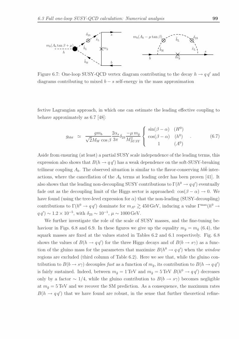
6.3 Full one-loop SUSY-QCD calculation: Numerical analysis 99
h
b
bL
bR
sL
s
mb(Ab tanβ + µ)
δ23
mg
⊗
b
bR s
bL
sL
mg
mb(Ab − µ tanβ) δ23⊗ ⊗
Figure 6.7: One-loop SUSY-QCD vertex diagram contributing to the decay h→ q q′ and
diagrams contributing to mixed b− s self-energy in the mass approximation
fective Lagrangian approach, in which one can estimate the leading effective coupling to
behave approximately as 6.7 [48]:
ghbs ≃gmb√
2MW cosβ
2αs3π
δ23−µmg
M2SUSY
sin(β − α) (H0)
cos(β − α) (h0)
1 (A0)
. (6.7)
Aside from ensuring (at least) a partial SUSY scale independence of the leading terms, this
expression also shows that B(h→ q q′) has a weak dependence on the soft-SUSY-breaking
trilinear coupling Ab. The observed situation is similar to the flavor-conserving hbb inter-
actions, where the cancellation of the Ab terms at leading order has been proven [41]. It
also shows that the leading non-decoupling SUSY contributions to Γ(h0 → q q′) eventually
fade out as the decoupling limit of the Higgs sector is approached: cos(β − α) → 0. We
have found (using the tree-level expression for α) that the non-leading (SUSY-decoupling)
contributions to Γ(h0 → q q′) dominate for mA0 & 450GeV, inducing a value Γmax(h0 →q q′) ∼ 1.2× 10⁻⁵, with δ23 ∼ 10−1, µ ∼ 1000GeV.
We further investigate the role of the scale of SUSY masses, and the fine-tuning be-
haviour in Figs. 6.8 and 6.9. In these figures we give up the equality mg = mq (6.4), the
squark masses are fixed at the values stated in Tables 6.2 and 6.1 respectively. Fig. 6.8
shows the values of B(h → q q′) for the three Higgs decays and of B(b → sγ) as a func-
tion of the gluino mass for the parameters that maximize B(h0 → q q′) when the window
regions are excluded (third column of Table 6.2). Here we see that, while the gluino con-
tribution to B(b→ sγ) decouples fast as a function of mg, its contribution to B(h→ q q′)
is fairly sustained. Indeed, between mg = 1TeV and mg = 5TeV B(h0 → q q′) decreases
only by a factor ∼ 1/4, while the gluino contribution to B(b → sγ) becomes negligible
at mg = 5TeV and we recover the SM prediction. As a consequence, the maximum rates
B(h → q q′) that we have found are robust, in the sense that further theoretical refine-
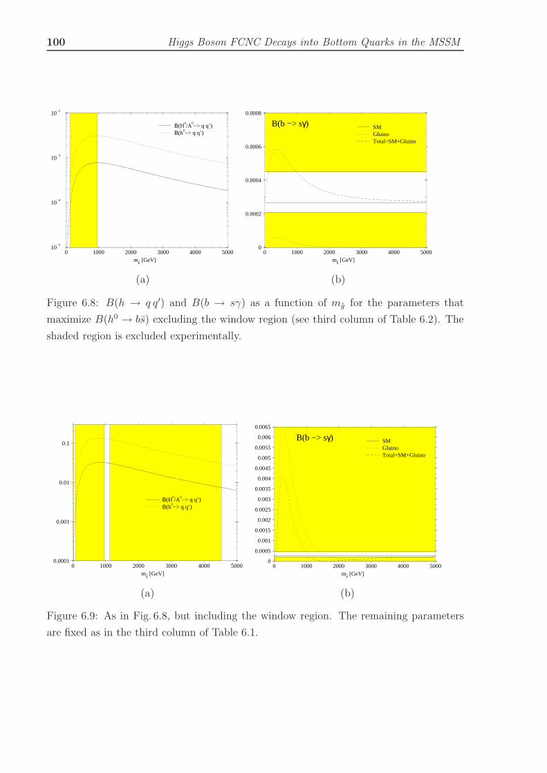
100 Higgs Boson FCNC Decays into Bottom Quarks in the MSSM
0 1000 2000 3000 4000 5000mg~ [GeV]
10−5
10−4
10−3
10−2
Β(H0/A
0−> q q’)
Β(h0−> q q’)
0 1000 2000 3000 4000 5000mg~ [GeV]
0
0.0002
0.0004
0.0006
0.0008
SMGluinoTotal=SM+Gluino
B(b −> sγ)
(a) (b)
Figure 6.8: B(h → q q′) and B(b → sγ) as a function of mg for the parameters that
maximize B(h0 → bs) excluding the window region (see third column of Table 6.2). The
shaded region is excluded experimentally.
0 1000 2000 3000 4000 5000mg~ [GeV]
0.0001
0.001
0.01
0.1
Β(H0/A
0−> q q’)
Β(h0−> q q’)
0 1000 2000 3000 4000 5000mg~ [GeV]
0
0.0005
0.001
0.0015
0.002
0.0025
0.003
0.0035
0.004
0.0045
0.005
0.0055
0.006
0.0065
SMGluinoTotal=SM+Gluino
B(b −> sγ)
(a) (b)
Figure 6.9: As in Fig. 6.8, but including the window region. The remaining parameters
are fixed as in the third column of Table 6.1.

6.3 Full one-loop SUSY-QCD calculation: Numerical analysis 101
Particle H0 h0 A0
Γ(GeV) B(h→ q q′) Γ(GeV) B(h→ q q′) Γ(GeV) B(h→ q q′)
small-αeff
window11.0 3.3× 10⁻² 1.6× 10⁻³ 1.3× 10⁻¹ 11.3 3.3× 10⁻²
tree-Higgs
window11.3 3.3× 10⁻² 5.4× 10⁻³ 4.3× 10⁻³ 11.3 3.3× 10⁻²
small-αeff
no-window11.2 9.1× 10⁻⁴ 1.4× 10⁻³ 3.1× 10⁻³ 11.3 9.0× 10⁻⁴
tree-Higgs
no-window 11.3 9.1× 10⁻⁴ 5.4× 10⁻³ 1.3× 10⁻⁴ 11.3 9.0× 10⁻⁴
tan β = 5 0.11 2.0× 10⁻³ 6.0× 10⁻³ 1.7× 10⁻⁴ 0.11 2.1× 10⁻³
tanβ = 5
tree Higgs0.12 1.9× 10⁻³ 4.4× 10⁻³ 2.6× 10⁻⁴ 0.11 2.1× 10⁻³
tanβ = 5
no-window0.15 3.8× 10⁻⁴ 9.7× 10⁻³ 1.1× 10⁻⁴ 0.11 5.1× 10⁻⁴
Table 6.4: Maximum values of B(h→ q q′) and corresponding Γ(h→ X) for the different
scenarios studied in this work.
ments and experimental results that change the allowed range of B(b → sγ) can easily
be compensated for by a slight increase of the gluino mass (mg), which would leave the
prediction for B(h → q q′) essentially unchanged. We note in Fig. 6.9 the correspond-
ing behaviour of B(h0 → q q′) and B(b → sγ) in the presence of fine-tuning, i.e. as
in Table 6.1. In contrast to the previous case, here we observe the presence of two tiny
windows in the regions mg = 25 − 75GeV and mg = 950 − 1125GeV. In the middle
region mg = 75− 950GeV, B(b→ sγ) is one order of magnitude larger than the allowed
experimental range, and in the region above mg = 1125GeV it only enters the allowed
region for mg > 4500GeV. In this region B(h0 → q q′) is still large, but at the price of
having a gluino five times heavier than the rest of the SUSY spectrum. This is another
manifestation of the large fine-tuning that governs this region of the parameter space.
Up to this point we have used the high tanβ value quoted in Eq. (6.4). But we have
also looked at the impact of varying tanβ on Bmax(h → q q′). Since the latest LEP
data restricts tanβ & 2.5, we have used a moderate value of tanβ = 5. Note that, at low
tan β, the small αeff scenario does not arise. As a consequence similar results are obtained
using either the tree-level or one-loop expressions for the Higgs sector parameters. We

102 Higgs Boson FCNC Decays into Bottom Quarks in the MSSM
find that the three branching ratios Bmax(h → q q′) at tanβ = 5 stay in the same order
of magnitude as in the scenarios with tanβ = 50 (default case) with the tree-level Higgs
sector and no-window (Cf. Table 6.2).
6.4 Remarks and conclusions
The main numbers of our analysis are put in a nutshell in Table 6.4, where we show the
results presented previously, together with some other scenarios and the low tan β case.
The computed maximum values of B(h → q q′) must not be taken as exact numbers
in practice, but order of magnitude results. The implications that can be derived from
Table 6.4 can be synthesized as follows:
1. The SUSY-QCD contributions can enhance the maximum expectation for the FCNC
decay rates B(h → q q′) enormously. This is seen by comparing the results of
Table 6.4 with the maximum value of B(HSM → bs) considered in Eq. (1.5). The
optimized MSSM branching ratios are at the very least 3 orders of magnitude bigger
than the SM result.
2. If no special circumstances apply, that is, if no fine-tuning occurs between the param-
eters contributing to B(b→ sγ) in the MSSM, and if Γ(h0 → bb) is not suppressed,
the maximum rates are Bmax(h0 → q q′) ≃ 1.3 × 10⁻⁴, Bmax(H0/A0 → q q′) ≃9× 10⁻⁴. This corresponds to the tree-Higgs/no-window scenario in Table 6.4.
3. If, however, Γ(h0 → bb) is suppressed by the radiative corrections to the CP-even
mixing angle α, then B(h0 → q q′) can be an order of magnitude larger: Bmax(h0 →q q′) ∼ 3 × 10⁻³. This corresponds to the small αeff scenario, and is indicated by
small-αeff/ no-window in Table 6.4. The FCNC branching ratio that we find for h0
in this case should be considered as the largest possible one within the conditions
of naturalness (no fine-tuning).
4. On the other hand, if fine-tuning between the gluino and the SM contributions to
B(b → sγ) is allowed, but the small-αeff scenario is not realized, then Bmax(h0 →q q′) grows one order of magnitude up to Bmax(h0 → q q′) ∼ 4 × 10⁻³, whereas
Bmax(H0/A0 → q q′) ∼ 3 × 10⁻². This corresponds to the case labelled tree-
Higgs/window in Table 6.4.
5. When both special conditions take place simultaneously, viz. fine-tuning in B(b→sγ) (triggered by a very special choice of the δ23 parameter in a narrow window

6.4 Remarks and conclusions 103
range) and small αeff scenario (independent of assumptions on δ23), we reach an
over-optimistic situation where Bmax(h0 → q q′) could reach the ∼ 10% level. This
is the case referred to as small-αeff/ window in Table 6.4.
6. If tan β is low/moderate, then Bmax(h→ q q′) lie in the lower range ∼ 10−4, which
can grow an order or magnitude for Bmax(H0/A0 → q q′) in fine-tuned scenarios
(last three rows in Table 6.4).
Although the large FCNC rates mentioned in points 4 and 5 above seem to offer
a rather tempting perspective, we will not elaborate on them any further since in our
opinion the fine-tuning requirement inherent in them is too contrived. On the other
hand, points 2 and 3 offer a moderate, but certainly much more realistic scenario, which
in no way frustrates our hopes to potentially detect the FCNC Higgs boson decays (6.1).
Indeed, in the case described in point 2, B(h → q q′) can be at most of order 10−4. But
this is still a fairly respectable FCNC branching ratio (comparable to that of b→ sγ) and
it may lead to a large number of events at a high luminosity collider as seen in chapter 7
for the MSSM and the chapter 4 for the general 2HDM. Moreover, if Γ(h→ X) becomes
suppressed (e.g. by realizing the small αeff scenario, point 3) then B(h0 → q q′) can be
enhanced by an additional order of magnitude.
Our analysis correlates the values of B(h→ q q′) with that of B(b→ sγ), taking into
account only the SUSY-QCD contributions due to flavor mixing parameters among the
left-chiral squarks. The presence of several other competing contributions to B(b → sγ)
alters the borders of the allowed parameter space:
• For the fine-tuned scenarios, the presence and position of the allowed window regions
in the parameter space depends significantly on all the contributions, and therefore
also does the maximum value of B(h → q q′). Outside the window regions, the
computed value of B(b → sγ) can only be made consistent with the experimental
range, by means of a large splitting between the squark and gluino masses.
• For the non-fine-tuned scenarios, the inclusion of further contributions to B(b→ sγ)
also alters the allowed parameter space, but the condition of non-fine-tuning ensures
precisely that the change in the allowed range of δ23 is smooth, and the corresponding
change in Bmax(h→ q q′) is not dramatic.
Of course, the question immediately arises on what will happen if the data from present
B-meson factories further constrains the δ23 parameter. In that case, we should take into
account the (charged-current induced) SUSY-EW contributions to B(h→ q q′), see [49]).
However, we can advance that the SUSY-EW effects on Bmax(h→ q q′) that we find are in

104 Higgs Boson FCNC Decays into Bottom Quarks in the MSSM
the ballpark of Bmax(h0 → q q′) ∼ 3×10⁻⁵ and Bmax(H0/A0 → q q′) ∼ 1×10⁻⁵ for a non-
fine-tuned scenario, while Bmax(h0 → q q′) ∼ 2×10⁻⁴ and Bmax(H0/A0 → q q′) ∼ 8×10⁻⁵
for a fine-tuned scenario. From the analysis of the chapter 5 we expect that even with
these impoverished MSSM rates the number of FCNC events of that sort should be non-
negligible at the LHC.
Even though we have detected the existence of corners of the MSSM parameter space
where a Higgs boson FCNC branching ratio can barely reach the 10% level (cf. the narrow
windows in Fig. 6.3 and Fig. 6.9), we insist once more that they should be considered
rather unlikely as they are associated to fine tuning of the parameters and excluded
experimentally [102]. Moreover, in contrast to Ref [47], we find that it is the lightest
CP-even state, h0, the one that could have the largest FCNC branching ratio.
To conclude, we have presented a first realistic estimate of the branching ratios of
the Higgs boson FCNC decays (6.1) within the MSSM, assuming that the SUSY-QCD
corrections can be as large as permitted by the experimental constraints on B(b → sγ).
We have carried out a systematic and self-consistent maximization of the branching ratios
(6.2) taking into account this crucial experimental constraint. At the end of the day the
results that we obtain, especially for the lightest CP-even Higgs boson of the MSSM,
are fairly large: Bmax(h0 → q q′) ∼ 10−4 − 10−3. These MSSM rates turn out to be
between three to four orders of magnitude larger than the maximum SM rate (1.5), but
not five or six orders as naive expectations indicated. Whether this branching ratio is
measurable at the LHC [13,14] or at a high energy e+e− Linear Collider [15] can only be
established by means of specific experimental analyses. However, on the basis of related
studies in the general 2HDM (chapter 5) and from the MSSM (chapter 7), we can foresee
that an important number of FCNC events (6.1) can be potentially collected at the LHC.
They could play a complementary, if not decisive, role in the identification of low-energy
Supersymmetry. In this work we have dealt only with the maximum rates induced by the
SUSY-QCD sector of the model.

Chapter 7
Production and FCNC decay of
MSSM Higgs bosons into heavy
quarks in the LHC
7.1 Introduction
The rareness of the FCNC Higgs boson decay modes, as seen in the previous chapter 6
are an ideal laboratory to look for non-standard interactions superimposed onto the SM
ones. Similar considerations apply to the FCNC processes associated to the Hbs vertex,
but in this case it is more difficult to pin down the phenomenological signatures. Some
work along these lines has already been done, both in the MSSM (see chapter 6 and
Refs. [43, 45–50]) and in the general two-Higgs-doublet model (2HDM) (see chapters 4
and 5 and Refs. [51, 64]), and also in other extensions of the SM– see [25] for a review.
Up to now, the main effort has been concentrated in computing the FCNC decay modes at
one-loop within the new physics, and also in getting a realistic estimate of the maximum
branching ratios expected. It is not enough to compute the FCNC branching ratios in, say
the MSSM, and then evaluate them in some favorable region of the parameter space, for
one has to preserve at the same time the stringent bounds on other observables in which
the same physics can be applied, like the aforementioned low-energy b→ sγ decay. This
kind of correlated study was done very carefully in chapter 6 for the specific Higgs boson
FCNC decays into bottom quarks within the MSSM, h → b s (h = h0, H0, A0). In this
work we extend the latter work by computing also the top quark Higgs boson FCNC decay
modes of the heavy MSSM Higgs bosons, h→ t c (h = H0, A0) under the same restrictions
(recall that h0 cannot participate in this decay because mh0 < mt in the MSSM [11]).
105

106 Production and FCNC decay of MSSM Higgs bosons into heavy quarks in the LHC
Furthermore, in this work we carry out an additional step absolutely necessary to make
contact with experiment, namely we combine the FCNC decay branching ratios of the
MSSM Higgs bosons (into both top and bottom quarks) with their MSSM production
cross-sections in order to estimate the maximum number of FCNC events expected at
LHC energies and luminosities. Only in this way one can assess in a practical way the
probability of detecting such processes at the LHC. This computation was done for the
general 2HDM in chapter 5, but to the best of our knowledge the corresponding calculation
in the MSSM case is not available. In this work we perform this calculation and compare
the FCNC results obtained for the MSSM and 2HDM scenarios.
The relevant observable quantity on which we shall focus hereafter is the cross-section
for the production of electrically neutral pairs of heavy quarks of different flavors at the
LHC, whose origin stems from the FCNC decays of the neutral Higgs bosons of the MSSM,
h = h0, H0, A0 [6, 11]. Thus, we aim at the quantity
σ(pp→ h→ q q′) ≡ σ(pp→ hX)B(h→ q q′) ≡ σ(pp→ hX)Γ(h→ q q′)
Γ(h→ X)
≡ σ(pp→ hX)Γ(h→ q q′ + q q′)∑
i Γ(h→ Xi)(qq′ ≡ bs or tc) . (7.1)
Here Γ(h → X) is the – consistently computed – total width in each case. In order to
asses the possibility to measure these processes at the LHC, we have performed a scan
of the MSSM parameter space to find the maximum possible value of the production
rates (7.1) under study. The computation of the combined production rate is necessary,
since the correlations among the different factors are important. For example, in chap-
ter 6 it was shown that the maximum branching ratio for the lightest MSSM Higgs boson,
B(h0 → bs), is obtained in the regions of the parameter space where the coupling h0 b b
is strongly suppressed by quantum effects. On the other hand, the associated production
σ(pp→ h0bb) is one of the leading processes for the production of the lightest MSSM Higgs
boson. It is clear then that, in the regions where B(h0 → bs) is largest, σ(pp→ h0bb) will
be suppressed. Therefore, the maximum FCNC production rate at the LHC can only be
obtained by the combined analysis of the two relevant factors in (7.1) (viz. the branching
ratio and the Higgs boson production cross-section). We will see that the effects from
each factor are different in different regions of the parameter space. Moreover, the real-
istic production FCNC rates (7.1) in the MSSM parameter space can be obtained only
by including the restrictions imposed by the simultaneous analysis of the branching ratio
of the low-energy process b → s γ, whose range of values is severely limited by experi-
ment [52–58]. As in chapter 6, in this work we limit ourselves to supersymmetric FCNC
interactions mediated by the strongly interacting sector of the MSSM, i.e. the SUSY-QCD

7.2 General setting for the numerical analysis 107
flavor-violating interactions induced by the gluinos. The corresponding analysis for the
electroweak supersymmetric FCNC effects requires a lengthy separate presentation, and
will be reported elsewhere [159].
The work is organized as follows. In Section 7.2 we describe the general setting for our
numerical analysis. In Section 7.3 we present the LHC production rates of Higgs boson
decaying into bottom quarks through supersymmetric FCNC interactions. In Section 7.4
we present the corresponding FCNC rates for the top quark channel. Finally, in Section 7.5
we compare the MSSM results with the 2HDM results, and deliver our conclusions.
7.2 General setting for the numerical analysis
We have performed the calculations with the help of the numeric programs HIGLU, PPHTT [136,
139,151,160] and LoopTools [129,161,162]. The calculation must obviously be finite with-
out renormalization, and indeed the cancellation of UV divergences using either dimen-
sional regularization or dimensional reduction – the two methods giving the same results
here – in the total amplitudes was verified explicitly. In the following we will detail the
approximations used in our computation:
• We include the full one-loop SUSY-QCD contributions to the FCNC partial decay
widths Γ(h→ q q′) in the observable (7.1).
• We assume that FCNC mixing terms appear only in the LH-chiral sector of the
6× 6 squark mixing matrix. Therefore, this matrix has only non-diagonal blocks in
the LH-LH sector. This is the most natural assumption from the theoretical point
of view [93], and, moreover, it was proven in Ref. [43] that the presence of FCNC
terms in the RH-chiral sector would enhance the partial widths by a factor two at
most – not an order of magnitude.
• The Higgs sector parameters (masses and CP-even mixing angle α) have been
treated using the leading mt and mb tan β approximation to the one-loop result [85,
154–156]. For comparison, we also perform the analysis using the tree-level approx-
imation.
• The Higgs bosons total decay widths Γ(h → X) are computed at leading order,
including all the relevant channels: Γ(h→ f f , ZZ,W+W−, gg). The off-shell decays
Γ(h → ZZ∗,W±W∓∗) have also been included. This is necessary to consistently
compute the total decay width of Γ(h0 → X) in regions of the parameter space
where the maximization of the cross-section (7.1) is obtained at the expense of
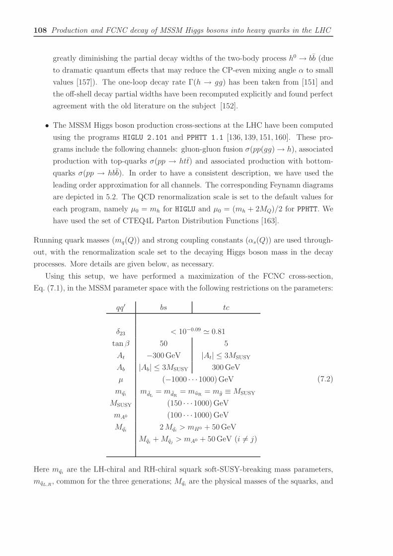
108 Production and FCNC decay of MSSM Higgs bosons into heavy quarks in the LHC
greatly diminishing the partial decay widths of the two-body process h0 → bb (due
to dramatic quantum effects that may reduce the CP-even mixing angle α to small
values [157]). The one-loop decay rate Γ(h → gg) has been taken from [151] and
the off-shell decay partial widths have been recomputed explicitly and found perfect
agreement with the old literature on the subject [152].
• The MSSM Higgs boson production cross-sections at the LHC have been computed
using the programs HIGLU 2.101 and PPHTT 1.1 [136, 139, 151, 160]. These pro-
grams include the following channels: gluon-gluon fusion σ(pp(gg)→ h), associated
production with top-quarks σ(pp → htt) and associated production with bottom-
quarks σ(pp → hbb). In order to have a consistent description, we have used the
leading order approximation for all channels. The corresponding Feynamn diagrams
are depicted in 5.2. The QCD renormalization scale is set to the default values for
each program, namely µ0 = mh for HIGLU and µ0 = (mh + 2MQ)/2 for PPHTT. We
have used the set of CTEQ4L Parton Distribution Functions [163].
Running quark masses (mq(Q)) and strong coupling constants (αs(Q)) are used through-
out, with the renormalization scale set to the decaying Higgs boson mass in the decay
processes. More details are given below, as necessary.
Using this setup, we have performed a maximization of the FCNC cross-section,
Eq. (7.1), in the MSSM parameter space with the following restrictions on the parameters:
qq′ bs tc
δ23 < 10−0.09 ≃ 0.81
tan β 50 5
At −300GeV |At| ≤ 3MSUSY
Ab |Ab| ≤ 3MSUSY 300GeV
µ (−1000 · · ·1000)GeV
mqi mdL= mdR
= muR= mg ≡MSUSY
MSUSY (150 · · ·1000)GeV
mA0 (100 · · ·1000)GeV
Mqi 2Mqi > mH0 + 50GeV
Mqi +Mqj > mA0 + 50GeV (i 6= j)
(7.2)
Here mqi are the LH-chiral and RH-chiral squark soft-SUSY-breaking mass parameters,
mqL,R, common for the three generations; Mqi are the physical masses of the squarks, and

7.2 General setting for the numerical analysis 109
mh is the mass of the decaying Higgs boson h = h0, H0, A0. These masses are fixed at the
tree-level by the values of (tanβ,mA0) and the SM gauge boson masses and couplings [6].
Due to the structure of the Yukawa couplings in the MSSM, the value of tanβ is fixed at
a high (small) value for the bottom (top) quark channel as indicated. The parameter mA0
(the mass of the CP-odd Higgs boson) is assumed to vary in the range indicated in (7.2).
At one loop these masses receive corrections from the various SUSY fields, and therefore
depend on the values of the remaining parameters in Eq. (7.2). The characteristic SUSY
mass scale MSUSY defines the typical mass of the squark and gluino masses 1. The rest
of the parameters of the squark sector are determined by this setup. For instance, by
SU(2) gauge invariance we have muL= mdL
. Following the same notation as in [43], the
parameter δ23 represents the mixing between the second and third generation of LH-chiral
squarks. Let us recall its definition:
δ23 ≡m2bLsL
mbLmsL
, (7.3)
m2bLsL
being the non-diagonal term in the squark mass matrix squared mixing the second
and third generation of LH-chiral squarks – and an equivalent definition for the up-type
quarks.2 The parameter δ23 is a fundamental quantity in our analysis as it determines
the strength of the tree-level FCNC interactions induced by the supersymmetric strong
interactions, which are then transferred to the loop diagrams of the Higgs boson FCNC
decays in Eq. (7.1). The last two restrictions in Eq. (7.2) ensure that the (heavy) Higgs
boson decay channels into a pair of squarks are kinematically forbidden. We have checked
explicitly for some of the heavy Higgs boson channels (h0 can never do it in practice)
that we obtain the same results if we remove these conditions and include the partial
widths Γ(h→ qq∗) in the denominator of (7.1). Strictly speaking this condition could be
implemented, in the case of the H0 boson, by just requiring mH0 < 2Mqi, but we have
made it stronger by including an additive term. This term is arbitrary (provided it is not
very small) and acts as a buffer, namely it impedes that by an appropriate choice of the
squark masses we can approach arbitrarily close the threshold from above, and therefore
avoids artificial enhancement effects in our loop calculations (see below). Similarly, for the
CP-odd Higgs boson, the condition expressed in (7.2) ensures that we avoid a similar kind
of enhancement. In this case, however, the condition is a bit different because the A0 qq∗
1Our programs are able to deal with completely arbitrary masses for each squark, but we are forced
to make some simplifications in order to provide a reasonable analysis within a manageable total CPU
time, see below.2Recall that the δij parameters in the up-sector are related to the corresponding parameters in the
down-sector by the Cabibbo-Kobayashi-Maskawa matrix, see e.g. [95, 96].

110 Production and FCNC decay of MSSM Higgs bosons into heavy quarks in the LHC
vertex can only exist with squarks of different chirality types (A0 qLqR∗) or, equivalently,
with different mass eigenstates (A0 qiqj∗). We have used fixed values for the soft-SUSY-
breaking trilinear couplings At and Ab for the bs and tc channels respectively. Our results
are essentially independent of these values and their signs.
The task of scanning the MSSM parameter space in order to maximize σ(pp → h →q q′) for the various Higgs bosons is quite demanding and highly CPU-time consuming,
even under the conditions imposed in Eq. (7.2). As stated in the introduction, our code
includes also the restrictions on the MSSM parameter space due to the experimental
constraint on B(b→ sγ), and therefore contains the full one-loop SUSY-QCD amplitude
for b → sγ constructed from the FCNC interactions induced by the gluinos. The scan
was carried out with the help of two entirely different methods. In the first method
we used a systematic procedure based on dividing the parameter subspace (7.2) into a
lattice which we filled with points distributed in a completely homogeneous way. The
second is a Monte-Carlo based method, first proposed in [164]. We have adapted the well-
known Vegas integration program [165] to generate a sufficient number of “interesting”
points in our parameter subspace. The total number of points used in this case was far
smaller than in the first method. Obviously the lattice procedure gives more accurate
results by increasing arbitrarily the total number of points, but the CPU time becomes
prohibitively long for the whole analysis. This is so even after factoring out in a suitable
way the phase-space integrals of the Higgs boson production processes, so that these
integrals are computed only once for every fixed Higgs boson mass and for all the MSSM
points of our scan in the parameter subspace (7.2). The second method is comparatively
much faster, but it still involves a quite respectable amount of CPU time for the whole
analysis. We found that the partial results obtained by the two methods are compatible
at the level of 10− 20%. For the study of our FCNC processes we consider that this level
of accuracy should be acceptable, and for this reason all of the plots that we present in
this work have been finally computed with the Vegas-based procedure. This also explains
the wiggling appearance observed in the profiles of the curves presented in Sections 3-4.
For any given abscissa point in each one of these curves, the corresponding value on the
vertical (ordinate) axis is somewhere within a band whose width lies around 10− 20% of
the central value.
A few words on the effects of the B(b→ sγ) constraint in our analysis are now in order.
The SUSY-QCD contribution to B(b→ sγ) can be quite large, in fact as large as the SM
one, and with any sign. This raises the possibility of “fine-tuning” between the two type
of contributions in certain (narrow) regions of the parameter space. As a consequence we
could highly optimize our FCNC rates in these regions without being in conflict with the

7.3 Analysis of the bottom-strange channel 111
experimentally measured B(b → sγ) band. We have checked that in these regions the
number of FCNC events can be artificially augmented by one or two orders of magnitude.
Our scanning procedure indeed finds automatically these fine-tuning domains. However,
we have systematically avoided them in the presentation of our analysis (for more details
see chapter 6). In all of our plots, therefore, we show the results obtained for the non-
fine-tuned case only. We adopt B(b → sγ) = (2.1 − 4.5) × 10−4 as the experimentally
allowed range within three standard deviations [19].
7.3 Analysis of the bottom-strange channel
The main result of the numerical scan for the bottom channel is shown in Fig. 7.1. To
be specific: Fig. 7.1a shows the maximum values of the production cross-sections σ(pp→h → q q′) for the three MSSM Higgs bosons h = h0, H0, A0 at the LHC, as a function of
mA0 ; Fig. 7.1b displays the cross-section as a function of tanβ. In this plot we indicate the
value of σ(pp→ h→ q q′) (in pb) in the left-vertical axis, and at the same time we track
number of FCNC events (per 100 fb−1 of integrated luminosity) on the right vertical axis.
Looking at Fig. 7.1 one can see immediately that at large tanβ: i) the maximum number
of events is remarkably high (106 events!) for a FCNC process; ii) there is a sustained
region in the h0 channel, comprising the interval 300GeV . mA0 . 900GeV, with a flat
value of 5× 10³ events; iii) the chosen value of tan β = 50 is not critical for H0 and A0 as
long it is larger than 10. In Fig. 7.1b we see that the dependence on tanβ is essentially
the same for H0 and A0, but for h0 it is quite different: in the region 10 . tan β . 30 the
cross-section remains below 10−2 pb, but for tan β > 30 it starts climbing fast up to 0.3 pb
at tanβ = 50. The number of events here reaches a few times 104 for all channels (for
fixed mA0 = 200GeV) 3. For further reference, in Table 7.1 we show the numerical values
of σ(pp → h → q q′) together with the parameters which maximize the production for
tan β = 50 and mA0 = 200GeV. We include the value of B(h→ bs) at the maximization
point of the FCNC cross-section. We notice that at this point the lightest Higgs boson h0
is the one having the smallest branching ratio. This is in contrast to the situation when
one maximizes the branching ratios independently of the number of events as in chapter 6.
In Fig. 7.2a we show the effect on σ(pp → h0 → b s), and on the total decay width
Γ(h0 → X), of using the Higgs boson sector at the tree-level or at one-loop in our com-
putation. It is well-known that the h0 couplings to quarks are particularly sensitive to
this issue, and for this reason we focus on the lightest CP-even Higgs boson for these
3As already advertised, in reading the plots and tables in this work, one must keep in mind that they
are the result of a Monte-Carlo sampling near the region of the maximal values.
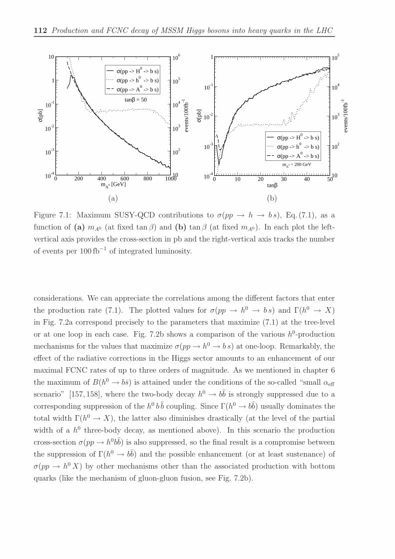
112 Production and FCNC decay of MSSM Higgs bosons into heavy quarks in the LHC
0 200 400 600 800 1000m
A0 [GeV]
10-4
10-3
10-2
10-1
1
10
σ[pb
]
10
102
103
104
105
106
even
ts/1
00fb-1
σ(pp -> H0 -> b s)
σ(pp -> h0 -> b s)
σ(pp -> A0 -> b s)
tanβ = 50
0 10 20 30 40 50tanβ
10-4
10-3
10-2
10-1
1
σ[pb
]
10
102
103
104
105
even
ts/1
00fb-1
σ(pp -> H0 -> b s)
σ(pp -> h0 -> b s)
σ(pp -> A0 -> b s)
mA
0 = 200 GeV
(a) (b)
Figure 7.1: Maximum SUSY-QCD contributions to σ(pp → h → b s), Eq. (7.1), as a
function of (a) mA0 (at fixed tanβ) and (b) tan β (at fixed mA0). In each plot the left-
vertical axis provides the cross-section in pb and the right-vertical axis tracks the number
of events per 100 fb−1 of integrated luminosity.
considerations. We can appreciate the correlations among the different factors that enter
the production rate (7.1). The plotted values for σ(pp → h0 → b s) and Γ(h0 → X)
in Fig. 7.2a correspond precisely to the parameters that maximize (7.1) at the tree-level
or at one loop in each case. Fig. 7.2b shows a comparison of the various h0-production
mechanisms for the values that maximize σ(pp→ h0 → b s) at one-loop. Remarkably, the
effect of the radiative corrections in the Higgs sector amounts to an enhancement of our
maximal FCNC rates of up to three orders of magnitude. As we mentioned in chapter 6
the maximum of B(h0 → bs) is attained under the conditions of the so-called “small αeff
scenario” [157, 158], where the two-body decay h0 → bb is strongly suppressed due to a
corresponding suppression of the h0 b b coupling. Since Γ(h0 → bb) usually dominates the
total width Γ(h0 → X), the latter also diminishes drastically (at the level of the partial
width of a h0 three-body decay, as mentioned above). In this scenario the production
cross-section σ(pp→ h0bb) is also suppressed, so the final result is a compromise between
the suppression of Γ(h0 → bb) and the possible enhancement (or at least sustenance) of
σ(pp → h0X) by other mechanisms other than the associated production with bottom
quarks (like the mechanism of gluon-gluon fusion, see Fig. 7.2b).

7.3 Analysis of the bottom-strange channel 113
h H0 h0 A0
σ(pp→ h→ q q′) 0.45 pb 0.34 pb 0.37 pb
events/100 fb−1 4.5× 10⁴ 3.4× 10⁴ 3.7× 10⁴
B(h→ bs) 9.3× 10⁻⁴ 2.1× 10⁻⁴ 8.9× 10⁻⁴
Γ(h→ X) 10.9GeV 1.00GeV 11.3GeV
δ23 10−0.62 10−1.32 10−0.44
mq 990GeV 670GeV 990GeV
Ab −2750GeV −1960GeV −2860GeV
µ −720GeV −990GeV −460GeV
B(b→ sγ) 4.50× 10⁻⁴ 4.47× 10⁻⁴ 4.39× 10⁻⁴
Table 7.1: Maximum value of σ(pp → h → q q′) (and of the number of bs events per
100 fb−1) in the LHC, for mA0 = 200GeV and tanβ = 50. Shown are also the corre-
sponding values of the relevant branching ratio B(h → bs) and of the total width of the
Higgs bosons, together with the values of the SUSY parameters. The last row includes
B(b→ sγ).
0 200 400 600 800 1000m
A0 [GeV]
10-5
10-4
10-3
10-2
10-1
1
10
102
σ[pb
] , Γ
[GeV
]
1
10
102
103
104
105
106
107
even
ts/1
00fb-1
Γ(h0-> X)
σ(pp -> h0 -> b s)
Γ(h0-> X) tree-Higgs
σ(pp -> h0 -> b s) tree-Higgs
tanβ = 50
0 200 400 600 800 1000m
A0 [GeV]
10-4
10-3
10-2
10-1
1
10
102
103
104
σ[pb
]
σ(qq,gg -> h0 bb)
σ(gg -> h0)
σ(qq,gg -> h0 tt)
tanβ = 50
(a) (b)
Figure 7.2: (a) h0 production cross-section and decay width as a function of mA0 with
the Higgs mass relations at tree-level and at one-loop. (b) Different contributions to the
h0 production cross-section as a function of mA0 corresponding to the maximization of
σ(pp→ h0 → b s) using the one-loop Higgs mass relations.

114 Production and FCNC decay of MSSM Higgs bosons into heavy quarks in the LHC
Indeed, for mA0 . 300GeV we can check in Fig. 7.2b that the most relevant factor
for maximizing the FCNC cross-section is the enhancement of the h0 production channel
in association with bottom quarks, σ(pp→ h0bb). This channel operates through the bb-
fusion vertex bb→ h0 and is highly enhanced at large tanβ. In the region mA0 . 300GeV
stays as the dominant mechanism for h0 production, although one can see that the alter-
nate gg-fusion mechanism remains all the way non-negligible. The corresponding effect
on our FCNC cross-section (7.1) is nevertheless not obvious because this same parame-
ter choice does also maximize the total width of h0, mainly through the enhancement of
Γ(h0 → b b). There is a delicate interplay of various factors here. In particular, in the
region mA0 < 300GeV the maximized partial width of the FCNC process h0 → bs (which
is a function of all the parameters in (7.2)) is larger than in the region mA0 > 300GeV,
but at the same time the total width becomes smaller in the latter region. Overall, the
result is that σ(pp → h0 → b s) is larger in the former mA0 range than in the latter.
Furthermore, when we cross ahead the limit mA0 ≃ 300GeV the dominant h0-production
channel changes turn: the associated h0-production with bottom quarks falls abruptly
down (see explanations below) and the gluon-gluon fusion mechanism takes over, so that
in this range the h0-production cross-section becomes completely dominated by gg → h0.
We note that while this mechanism is not so efficient at its maximum as the associated
production, it has a virtue: it is non-suppressed in the entire range of mA0 . As a re-
sult, in the region above mA0 & 300GeV a small value of the h0 b b coupling enhances
B(h0 → bs) while it does not dramatically suppress the total cross-section σ(pp → hX).
For mA0 > 300GeV our sampling procedure finds the maximum by selecting the points
in parameter space corresponding to the small αeff scenario, where B(h0 → bs) takes
the highest values and Γ(h0 → X) and σ(pp→ h0bb) are strongly suppressed – the latter
staying below the associated Higgs boson production with top quarks! In this way the net
Higgs boson cross-section σ(pp→ h0) is not drastically reduced thanks to the sustenance
provided by the gg-fusion channel. Most of the loop contributions to it come from the top
quark because the bottom quark contribution is suppressed and the squarks are rather
heavy. One can clearly see this sustenance feature in Fig. 7.2 in the form of a long cross-
section plateau up to around mA0 = 1TeV, beyond which the small αeff scenario cannot
be maintained and Γ(h0 → X) starts increasing and at the same time σ(pp → h0 → b s)
starts decreasing. It is remarkable that this behavior is only feasible thanks to the large
radiative corrections in the MSSM Higgs sector. When we, instead, perform the computa-
tion using the tree-level relations for the Higgs sector, the small αeff scenario is obviously
not possible and the enhancements/suppressions of σ(pp → h0bb)/Γ(h0 → X) cannot
take place. As a result the FCNC rate is some 3 orders of magnitude smaller than in the

7.3 Analysis of the bottom-strange channel 115
-2 -1.5 -1 -0.5 0log δ
23
10-3
10-2
10-1
1
σ[pb
]
102
103
104
105
even
ts/1
00fb-1
σ(pp -> H0 -> b s)
σ(pp -> h0 -> b s)
σ(pp -> A0 -> b s)
tanβ = 50 mA
0 = 200 GeV
-2 -1.5 -1 -0.5 0log δ
23
2 x 10⁻⁴
3 x 10⁻⁴
4 x 10⁻⁴
5 x 10⁻⁴
B(b
->
s γ)
BH(b -> s γ)
Bh(b -> s γ)
BA(b -> s γ)
tanβ = 50
mA
0 = 200 GeV
(a) (b)
Figure 7.3: Maximum SUSY-QCD contributions to σ(pp → h → b s), Eq. (7.1), as a
function of (a) δ23 and (b) value of b→ sγ.
previous case.
Next, we turn our attention to the FCNC mixing parameter δ23 in Eq. (6.5). The
value of δ23 at the cross-section maximum is not necessarily the maximum allowed value
of δ23 in (7.2). This is because it is a conditioned maximum, namely a maximum obtained
under the restrictions imposed by b→ sγ, as illustrated in Fig. 7.3. For further reference
in our discussion, and to better grasp some qualitative features of our results, let us write
the general form of the SUSY-QCD contribution to b → sγ. If we emphasize only the
relevant supersymmetric terms under consideration (obviating the powers of the gauge
couplings and other factors) we have
B(b→ sγ) ∼ δ223 m
2b(At − µ tanβ)2/M4
SUSY . (7.4)
Fig. 7.3a shows the maximum of σ(pp → h → q q′) as a function of δ23 for a fixed value
of the CP-odd Higgs boson mass mA0 = 200GeV, whereas Fig. 7.3b shows the computed
value of B(b → sγ) corresponding to the parameter space points where each maximum
is attained. At small δ23 the SUSY-QCD contribution to B(b → sγ) is negligible, and
the experimental restriction B(b → sγ) = (2.1 − 4.5) × 10−4 does not place constraints
on the other MSSM parameters (7.2); in other words, in this region the dependence is
σ(pp → h → q q′) ∝ (δ23)2 – the naively expected one. Here δ23 . 10−1.5 ≃ 0.03 and
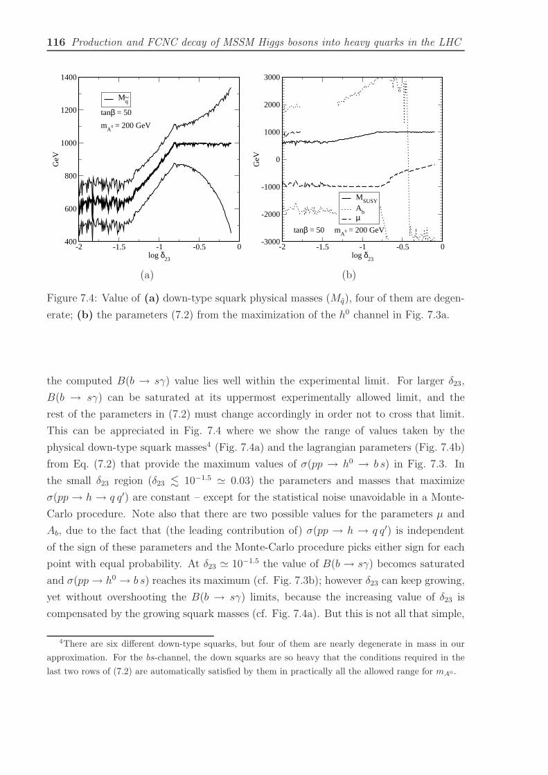
116 Production and FCNC decay of MSSM Higgs bosons into heavy quarks in the LHC
-2 -1.5 -1 -0.5 0log δ
23
400
600
800
1000
1200
1400
GeV
Mq~
tanβ = 50
mA
0 = 200 GeV
-2 -1.5 -1 -0.5 0log δ
23
-3000
-2000
-1000
0
1000
2000
3000
GeV
MSUSY
Ab
µtanβ = 50 m
A0 = 200 GeV
(a) (b)
Figure 7.4: Value of (a) down-type squark physical masses (Mq), four of them are degen-
erate; (b) the parameters (7.2) from the maximization of the h0 channel in Fig. 7.3a.
the computed B(b → sγ) value lies well within the experimental limit. For larger δ23,
B(b → sγ) can be saturated at its uppermost experimentally allowed limit, and the
rest of the parameters in (7.2) must change accordingly in order not to cross that limit.
This can be appreciated in Fig. 7.4 where we show the range of values taken by the
physical down-type squark masses4 (Fig. 7.4a) and the lagrangian parameters (Fig. 7.4b)
from Eq. (7.2) that provide the maximum values of σ(pp → h0 → b s) in Fig. 7.3. In
the small δ23 region (δ23 . 10−1.5 ≃ 0.03) the parameters and masses that maximize
σ(pp → h → q q′) are constant – except for the statistical noise unavoidable in a Monte-
Carlo procedure. Note also that there are two possible values for the parameters µ and
Ab, due to the fact that (the leading contribution of) σ(pp → h → q q′) is independent
of the sign of these parameters and the Monte-Carlo procedure picks either sign for each
point with equal probability. At δ23 ≃ 10−1.5 the value of B(b → sγ) becomes saturated
and σ(pp→ h0 → b s) reaches its maximum (cf. Fig. 7.3b); however δ23 can keep growing,
yet without overshooting the B(b → sγ) limits, because the increasing value of δ23 is
compensated by the growing squark masses (cf. Fig. 7.4a). But this is not all that simple,
4There are six different down-type squarks, but four of them are nearly degenerate in mass in our
approximation. For the bs-channel, the down squarks are so heavy that the conditions required in the
last two rows of (7.2) are automatically satisfied by them in practically all the allowed range for mA0 .
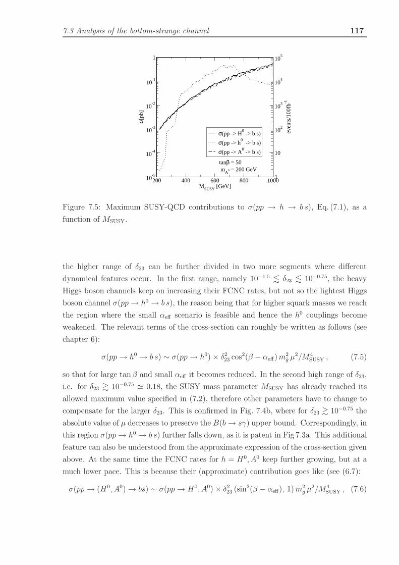
7.3 Analysis of the bottom-strange channel 117
200 400 600 800 1000M
SUSY [GeV]
10-5
10-4
10-3
10-2
10-1
1
σ[pb
]
10
1
102
103
104
105
even
ts/1
00fb-1
σ(pp -> H0 -> b s)
σ(pp -> h0 -> b s)
σ(pp -> A0 -> b s)
tanβ = 50m
A0 = 200 GeV
Figure 7.5: Maximum SUSY-QCD contributions to σ(pp → h → b s), Eq. (7.1), as a
function of MSUSY.
the higher range of δ23 can be further divided in two more segments where different
dynamical features occur. In the first range, namely 10−1.5 . δ23 . 10−0.75, the heavy
Higgs boson channels keep on increasing their FCNC rates, but not so the lightest Higgs
boson channel σ(pp→ h0 → b s), the reason being that for higher squark masses we reach
the region where the small αeff scenario is feasible and hence the h0 couplings become
weakened. The relevant terms of the cross-section can roughly be written as follows (see
chapter 6):
σ(pp→ h0 → b s) ∼ σ(pp→ h0)× δ223 cos2(β − αeff)m2
g µ2/M4
SUSY , (7.5)
so that for large tanβ and small αeff it becomes reduced. In the second high range of δ23,
i.e. for δ23 & 10−0.75 ≃ 0.18, the SUSY mass parameter MSUSY has already reached its
allowed maximum value specified in (7.2), therefore other parameters have to change to
compensate for the larger δ23. This is confirmed in Fig. 7.4b, where for δ23 & 10−0.75 the
absolute value of µ decreases to preserve the B(b→ sγ) upper bound. Correspondingly, in
this region σ(pp→ h0 → b s) further falls down, as it is patent in Fig 7.3a. This additional
feature can also be understood from the approximate expression of the cross-section given
above. At the same time the FCNC rates for h = H0, A0 keep further growing, but at a
much lower pace. This is because their (approximate) contribution goes like (see (6.7):
σ(pp→ (H0, A0)→ bs) ∼ σ(pp→ H0, A0)× δ223 (sin2(β − αeff), 1)m2
g µ2/M4
SUSY , (7.6)

118 Production and FCNC decay of MSSM Higgs bosons into heavy quarks in the LHC
similar to the h0 case but with angular dependences on αeff and β which are non-
suppressing in this region (see chapter 6). Again, any further increase of δ23 is now
partially cancelled by the b → sγ constraint, which demands smaller values of µ. This
explains the stabilization of the FCNC rates of the H0 and A0 channels in the highest δ23
range (cf. Fig. 7.3a). The profile of the squark mass curves in Fig. 7.4a implies a mixing
mass matrix with constant diagonal terms (with value MSUSY) and growing mixing terms
(δ23).
We finish our analysis of σ(pp→ h→ q q′) by looking at its behavior as a function of
the SUSY mass scale MSUSY, viz. the overall scale for the squark and gluino masses – cf.
Eq. (7.2). Fig. 7.5 shows the maximum of σ(pp → h → q q′) as a function of MSUSY for
fixed mA0 = 200GeV and tanβ = 50. The interpretation of this figure follows closely the
results of the previous ones. At small values of MSUSY the potentially large contribution
to B(b → sγ) has to be compensated – see Eq. (7.4) – by small values of δ23 and/or |µ|,resulting in a (relatively) small value of σ(pp → h → q q′). As MSUSY grows, δ23 and |µ|can take larger values without disturbing the restrictions from B(b → sγ). The leading
contribution to our FCNC cross-sections is actually independent of the overall SUSY mass
scale MSUSY, because for all Higgs boson channels we have found the general behavior
(leaving aside other terms mentioned above)
σ(pp→ h→ q q′) ∼ σ(pp→ h)× δ223 m
2g µ
2/M4SUSY (h = h0, H0, A0) . (7.7)
The last factor effectively behaves as δ223 µ
2/M2SUSY, and grows as δ2
23 for increasing MSUSY
at fixed ratio µ/MSUSY. Under the same conditions B(b→ sγ) causes no problem because
it is additionally suppressed by m2b/M
2SUSY – cf. Eq. (7.4). Therefore, we are led to a sort of
“non-decoupling behavior” of the FCNC rates with increasing MSUSY. In other words, we
find that for the heavy neutral Higgs bosons (H0, A0) the interesting region is (contrary to
naive expectations) the high MSUSY range! The lightest Higgs boson (h0) channel shows
a similar overall behavior, but it presents additional features because it is more tied to
the evolution of the CP-even mixing angle α. The most interesting region for this channel
is (cf. Fig. 7.5) the central squark mass scale MSUSY ∼ 600 − 800GeV, where the small
αeff scenario can take place.
From the combined analysis of Figs. 7.1-7.5 we arrive at the following conclusions
concerning the bs final state:
• A significant event rate of FCNC Higgs boson decays σ(pp→ h→ q q′) is expected
at the LHC, even after taking into account the limits on B(b→ sγ);
• Lightest Higgs boson case, h0:
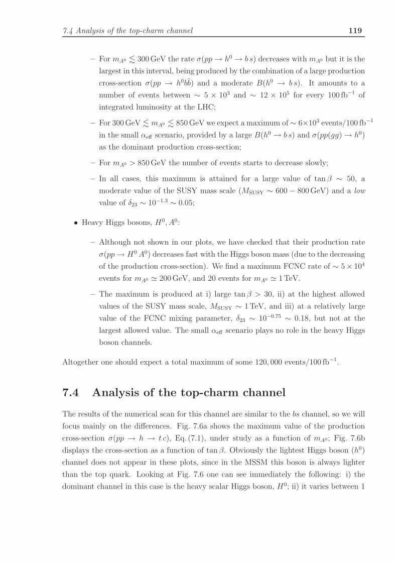
7.4 Analysis of the top-charm channel 119
– For mA0 . 300GeV the rate σ(pp→ h0 → b s) decreases with mA0 but it is the
largest in this interval, being produced by the combination of a large production
cross-section σ(pp → h0bb) and a moderate B(h0 → b s). It amounts to a
number of events between ∼ 5 × 10³ and ∼ 12 × 105 for every 100 fb−1 of
integrated luminosity at the LHC;
– For 300GeV . mA0 . 850GeV we expect a maximum of∼ 6×10³ events/100 fb−1
in the small αeff scenario, provided by a large B(h0 → b s) and σ(pp(gg)→ h0)
as the dominant production cross-section;
– For mA0 > 850GeV the number of events starts to decrease slowly;
– In all cases, this maximum is attained for a large value of tanβ ∼ 50, a
moderate value of the SUSY mass scale (MSUSY ∼ 600− 800GeV) and a low
value of δ23 ∼ 10−1.3 ∼ 0.05;
• Heavy Higgs bosons, H0, A0:
– Although not shown in our plots, we have checked that their production rate
σ(pp→ H0A0) decreases fast with the Higgs boson mass (due to the decreasing
of the production cross-section). We find a maximum FCNC rate of ∼ 5× 10⁴
events for mA0 ≃ 200GeV, and 20 events for mA0 ≃ 1TeV.
– The maximum is produced at i) large tanβ > 30, ii) at the highest allowed
values of the SUSY mass scale, MSUSY ∼ 1TeV, and iii) at a relatively large
value of the FCNC mixing parameter, δ23 ∼ 10−0.75 ∼ 0.18, but not at the
largest allowed value. The small αeff scenario plays no role in the heavy Higgs
boson channels.
Altogether one should expect a total maximum of some 120, 000 events/100 fb−1.
7.4 Analysis of the top-charm channel
The results of the numerical scan for this channel are similar to the bs channel, so we will
focus mainly on the differences. Fig. 7.6a shows the maximum value of the production
cross-section σ(pp → h → t c), Eq. (7.1), under study as a function of mA0 ; Fig. 7.6b
displays the cross-section as a function of tanβ. Obviously the lightest Higgs boson (h0)
channel does not appear in these plots, since in the MSSM this boson is always lighter
than the top quark. Looking at Fig. 7.6 one can see immediately the following: i) the
dominant channel in this case is the heavy scalar Higgs boson, H0; ii) it varies between 1
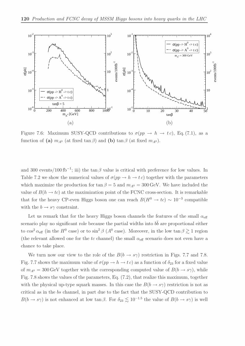
120 Production and FCNC decay of MSSM Higgs bosons into heavy quarks in the LHC
0 200 400 600 800 1000m
A0 [GeV]
10-6
10-5
10-4
10-3
10-2
σ[pb
]
10-1
1
10
102
103
even
ts/1
00fb-1
tanβ = 5
σ(pp -> H0 -> t c)
σ(pp -> A0 -> t c)
0 10 20 30 40 50tanβ
10-5
10-4
10-3
10-2
10-1
σ[pb
]
1
10
102
103
104
even
ts/1
00fb-1
σ(pp -> H0 -> t c)
σ(pp -> A0 -> t c)
mA
0 = 300 GeV
(a) (b)
Figure 7.6: Maximum SUSY-QCD contributions to σ(pp → h → t c), Eq. (7.1), as a
function of (a) mA0 (at fixed tan β) and (b) tanβ (at fixed mA0).
and 300 events/100 fb−1; iii) the tanβ value is critical with preference for low values. In
Table 7.2 we show the numerical values of σ(pp→ h→ t c) together with the parameters
which maximize the production for tanβ = 5 and mA0 = 300GeV. We have included the
value of B(h→ tc) at the maximization point of the FCNC cross-section. It is remarkable
that for the heavy CP-even Higgs boson one can reach B(H0 → tc) ∼ 10−3 compatible
with the b→ sγ constraint.
Let us remark that for the heavy Higgs boson channels the features of the small αeff
scenario play no significant role because the partial widths into bb are proportional either
to cos2 αeff (in the H0 case) or to sin2 β (A0 case). Moreover, in the low tan β & 1 region
(the relevant allowed one for the tc channel) the small αeff scenario does not even have a
chance to take place.
We turn now our view to the role of the B(b → sγ) restriction in Figs. 7.7 and 7.8.
Fig. 7.7 shows the maximum value of σ(pp→ h→ t c) as a function of δ23 for a fixed value
of mA0 = 300GeV together with the corresponding computed value of B(b→ sγ), while
Fig. 7.8 shows the values of the parameters, Eq. (7.2), that realize this maximum, together
with the physical up-type squark masses. In this case the B(b→ sγ) restriction is not as
critical as in the bs channel, in part due to the fact that the SUSY-QCD contribution to
B(b→ sγ) is not enhanced at low tanβ. For δ23 . 10−1.5 the value of B(b→ sγ) is well

7.4 Analysis of the top-charm channel 121
h H0 A0
σ(pp→ h→ t c) 2.4× 10⁻³ pb 5.8× 10⁻⁴ pb
events/100 fb−1 240 58
B(h→ tc) 1.9× 10⁻³ 5.7× 10⁻⁴
Γ(h→ X) 0.41GeV 0.39GeV
δ23 10−0.10 10−0.13
mq 880GeV 850GeV
At −2590GeV 2410GeV
µ −700GeV −930GeV
B(b→ sγ) 4.13× 10⁻⁴ 4.47× 10⁻⁴
Table 7.2: Maximum value of σ(pp → h → t c) (and of the number of tc events per
100 fb−1) in the LHC, for mA0 = 300GeV and tan β = 5. Shown are also the corre-
sponding values of the relevant branching ratio B(h → tc) and of the total width of the
Higgs bosons, together with the values of the SUSY parameters. The last row includes
B(b→ sγ).
inside the experimental limits (Fig. 7.7b), there is no restriction on the rest parameters
(Fig. 7.8b), the squark masses remain constant (Fig. 7.8a), and the maximum value of
σ(pp → h → t c) grows here in the naively expected way (δ23)2 (Fig. 7.7a). Above this
value (δ23 & 10−1.5) the parameters have to be adjusted to provide and acceptable range
for B(b→ sγ) 5. In this region the SUSY mass MSUSY grows (Fig. 7.8b), and |µ| decreases,
but not so fast as in the bs channel case (Fig. 7.4b). At the same time At increases with
increasing δ23 > 10−1.5. Most of the physical squark masses grow, but one of the up-type
squarks (stop squark) can always have the minimum allowed mass – Eq. (7.2). In this
region the observables under study grow more slowly, since their original δ223 behavior
is partially cancelled by the growing of MSUSY with δ23. In Fig. 7.9 we see, again, that
σ(pp → h → t c) grows with the SUSY mass scale (although in a way less pronounced
than in the bs channel), due to the relaxation of the b → sγ constraint for large MSUSY.
While σ(pp → h → q q′) is augmented nearly three orders of magnitude in the range
MSUSY = 200− 1000GeV (Fig. 7.5), the tc channel undergoes only an increase of roughly
5The two lines appearing in this region for BH(b→ sγ) mean that the maximum of σ(pp→ H0 → t c)
is attained either by the maximum or the minimum allowed value of B(b→ sγ), our Monte-Carlo sampling
procedure picks either choice with equal probability for each value of δ23.
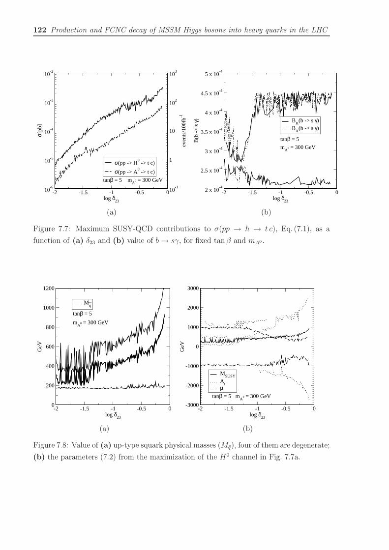
122 Production and FCNC decay of MSSM Higgs bosons into heavy quarks in the LHC
-2 -1.5 -1 -0.5 0log δ
23
10-6
10-5
10-4
10-3
10-2
σ[pb
]
10-1
1
10
102
103
even
ts/1
00fb-1
σ(pp -> H0 -> t c)
σ(pp -> A0 -> t c)
tanβ = 5 mA
0 = 300 GeV
-2 -1.5 -1 -0.5 0log δ
23
2 x 10⁻⁴
2.5 x 10⁻⁴
3 x 10⁻⁴
3.5 x 10⁻⁴
4 x 10⁻⁴
4.5 x 10⁻⁴
5 x 10⁻⁴
B(b
->
s γ) B
H(b -> s γ)
BA(b -> s γ)
tanβ = 5
mA
0 = 300 GeV
(a) (b)
Figure 7.7: Maximum SUSY-QCD contributions to σ(pp → h → t c), Eq. (7.1), as a
function of (a) δ23 and (b) value of b→ sγ, for fixed tan β and mA0 .
-2 -1.5 -1 -0.5 0log δ
23
0
200
400
600
800
1000
1200
GeV
Mq~
tanβ = 5
mA
0 = 300 GeV
-2 -1.5 -1 -0.5 0log δ
23
-3000
-2000
-1000
0
1000
2000
3000
GeV
MSUSY
At
µtanβ = 5 m
A0 = 300 GeV
(a) (b)
Figure 7.8: Value of (a) up-type squark physical masses (Mq), four of them are degenerate;
(b) the parameters (7.2) from the maximization of the H0 channel in Fig. 7.7a.
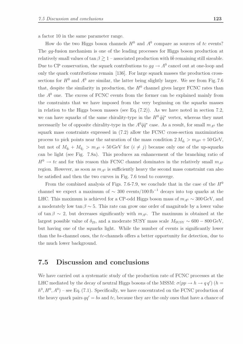
7.5 Discussion and conclusions 123
a factor 10 in the same parameter range.
How do the two Higgs boson channels H0 and A0 compare as sources of tc events?
The gg-fusion mechanism is one of the leading processes for Higgs boson production at
relatively small values of tanβ & 1 – associated production with bb remaining still sizeable.
Due to CP conservation, the squark contributions to gg → A0 cancel out at one-loop and
only the quark contributions remain [136]. For large squark masses the production cross-
sections for H0 and A0 are similar, the latter being slightly larger. We see from Fig. 7.6
that, despite the similarity in production, the H0 channel gives larger FCNC rates than
the A0 one. The excess of FCNC events from the former can be explained mainly from
the constraints that we have imposed from the very beginning on the squarks masses
in relation to the Higgs boson masses (see Eq. (7.2)). As we have noted in section 7.2,
we can have squarks of the same chirality-type in the H0 qq∗ vertex, whereas they must
necessarily be of opposite chirality-type in the A0qq∗ case. As a result, for small mA0 the
squark mass constraints expressed in (7.2) allow the FCNC cross-section maximization
process to pick points near the saturation of the mass condition 2Mqi > mH0 + 50GeV,
but not of Mqi + Mqj > mA0 + 50GeV for (i 6= j) because only one of the up-squarks
can be light (see Fig. 7.8a). This produces an enhancement of the branching ratio of
H0 → tc and for this reason this FCNC channel dominates in the relatively small mA0
region. However, as soon as mA0 is sufficiently heavy the second mass constraint can also
be satisfied and then the two curves in Fig. 7.6 tend to converge.
From the combined analysis of Figs. 7.6-7.9, we conclude that in the case of the H0
channel we expect a maximum of ∼ 300 events/100 fb−1 decays into top quarks at the
LHC. This maximum is achieved for a CP-odd Higgs boson mass of mA0 ∼ 300GeV, and
a moderately low tan β ∼ 5. This rate can grow one order of magnitude by a lower value
of tanβ ∼ 2, but decreases significantly with mA0 . The maximum is obtained at the
largest possible value of δ23, and a moderate SUSY mass scale MSUSY ∼ 600− 800GeV,
but having one of the squarks light. While the number of events is significantly lower
than the bs-channel ones, the tc-channels offers a better opportunity for detection, due to
the much lower background.
7.5 Discussion and conclusions
We have carried out a systematic study of the production rate of FCNC processes at the
LHC mediated by the decay of neutral Higgs bosons of the MSSM: σ(pp→ h→ q q′) (h =
h0, H0, A0) – see Eq. (7.1). Specifically, we have concentrated on the FCNC production of
the heavy quark pairs qq′ = bs and tc, because they are the only ones that have a chance of

124 Production and FCNC decay of MSSM Higgs bosons into heavy quarks in the LHC
200 400 600 800 1000M
SUSY [GeV]
10-5
10-4
10-3
10-2
σ[pb
]
10
1
102
103
even
ts/1
00fb-1
σ(pp -> H0 -> t c)
σ(pp -> A0 -> t c)
tanβ = 5m
A0 = 300 GeV
Figure 7.9: Maximum SUSY-QCD contributions to σ(pp → h → t c), Eq. (7.1), as a
function of MSUSY.
being detected. We have focused on the FCNC supersymmetric effects stemming from the
strongly interacting sector of the MSSM, namely from the gluino-mediated flavor-changing
interactions. We have performed a maximization of the event rates in the parameter space
under a set of conditions that can be considered “irreducible”, see Eq. (7.2), i.e. we cannot
further shorten this minimal set (e.g. by making additional assumptions on the relations
among the parameters) without potentially jeopardizing the conclusions of this study.
Even within this restricted parameter subspace the computer analysis has been rather
demanding. The numerical scan has been performed using Monte Carlo techniques which
we have partially cross-checked with more conventional methods. The maximization of the
cross-sections (7.1) has been performed by simultaneously computing the corresponding
MSSM quantum effects on the (relatively well-measured) low-energy FCNC decay b→ sγ
and requiring that the experimental limits on this observable are preserved.
To summarize our results: the total number of FCNC heavy flavor events originating
from supersymmetric Higgs boson interactions at the LHC can be large (of order 106), but
this does not mean that they can be easily disentangled from the underlying background
of QCD jets where they are immersed. For example, it is well known that the simple two-
body decay h→ b b is impossible to isolate due to the huge irreducible QCD background
from b b dijets – a result that holds for both the SM and the MSSM [13, 14]. This led a
long time ago to complement the search with many other channels, particularly h→ γ γ
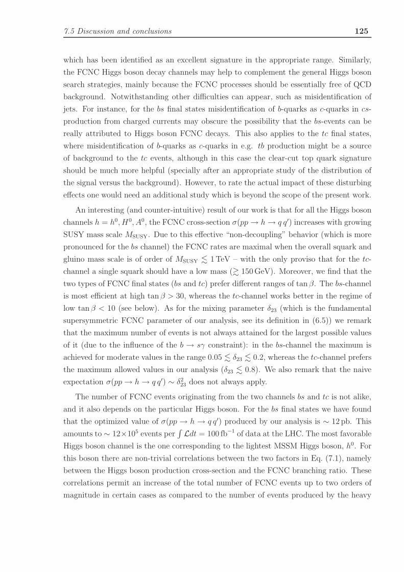
7.5 Discussion and conclusions 125
which has been identified as an excellent signature in the appropriate range. Similarly,
the FCNC Higgs boson decay channels may help to complement the general Higgs boson
search strategies, mainly because the FCNC processes should be essentially free of QCD
background. Notwithstanding other difficulties can appear, such as misidentification of
jets. For instance, for the bs final states misidentification of b-quarks as c-quarks in cs-
production from charged currents may obscure the possibility that the bs-events can be
really attributed to Higgs boson FCNC decays. This also applies to the tc final states,
where misidentification of b-quarks as c-quarks in e.g. tb production might be a source
of background to the tc events, although in this case the clear-cut top quark signature
should be much more helpful (specially after an appropriate study of the distribution of
the signal versus the background). However, to rate the actual impact of these disturbing
effects one would need an additional study which is beyond the scope of the present work.
An interesting (and counter-intuitive) result of our work is that for all the Higgs boson
channels h = h0, H0, A0, the FCNC cross-section σ(pp→ h→ q q′) increases with growing
SUSY mass scale MSUSY. Due to this effective “non-decoupling” behavior (which is more
pronounced for the bs channel) the FCNC rates are maximal when the overall squark and
gluino mass scale is of order of MSUSY . 1TeV – with the only proviso that for the tc-
channel a single squark should have a low mass (& 150GeV). Moreover, we find that the
two types of FCNC final states (bs and tc) prefer different ranges of tanβ. The bs-channel
is most efficient at high tan β > 30, whereas the tc-channel works better in the regime of
low tanβ < 10 (see below). As for the mixing parameter δ23 (which is the fundamental
supersymmetric FCNC parameter of our analysis, see its definition in (6.5)) we remark
that the maximum number of events is not always attained for the largest possible values
of it (due to the influence of the b → sγ constraint): in the bs-channel the maximum is
achieved for moderate values in the range 0.05 . δ23 . 0.2, whereas the tc-channel prefers
the maximum allowed values in our analysis (δ23 . 0.8). We also remark that the naive
expectation σ(pp→ h→ q q′) ∼ δ223 does not always apply.
The number of FCNC events originating from the two channels bs and tc is not alike,
and it also depends on the particular Higgs boson. For the bs final states we have found
that the optimized value of σ(pp → h → q q′) produced by our analysis is ∼ 12 pb. This
amounts to ∼ 12×105 events per∫
Ldt = 100 fb−1 of data at the LHC. The most favorable
Higgs boson channel is the one corresponding to the lightest MSSM Higgs boson, h0. For
this boson there are non-trivial correlations between the two factors in Eq. (7.1), namely
between the Higgs boson production cross-section and the FCNC branching ratio. These
correlations permit an increase of the total number of FCNC events up to two orders of
magnitude in certain cases as compared to the number of events produced by the heavy

126 Production and FCNC decay of MSSM Higgs bosons into heavy quarks in the LHC
Higgs bosons H0 and A0, which are essentially free of these correlations. The latter stem
from relevant quantum effects on the parameters of the Higgs boson sector at one-loop
precisely in the regions of our interest.
On the other hand, the maximum value of σ(pp → h → t c) is more moderate, to
wit: 3 × 10⁻³ pb, or ∼ 300 events/100 fb−1. For the total integrated luminosity during
the operative lifetime of the LHC, which amounts to some (300− 400) fb−1, we estimate
that a few thousand tc events could be collected in the most optimistic conditions. This
number is of course sensitive to many MSSM parameters, but most particularly to two:
mA0 and tan β. The mass of the CP-odd Higgs boson should not be heavier than mA0 ∼(400−500)GeV if one does not want to decrease the number of events below a few hundred
per 100 fb−1. On the other hand the number of events is very much dependent on the
particular range of tanβ. As we have said above, the lowest possible values are preferred
for the tc channel, but the sensitivity in this range is so high that the order of magnitude
of σ(pp → h→ t c) may change for different (close) choices of tanβ. Throughout all the
analysis of the tc channel we have fixed tanβ at an intermediate value, but the maximum
number of events per 100 fb−1 would grow from ∼ 300 (for our standard choice tanβ = 5)
up to ∼ (500, 900, 2000) if we would have chosen tanβ = (4, 3, 2) respectively. Such
lower values of tan β are usually avoided in some MSSM analyses in the literature, but
as a matter of fact there are no fully water-tight experimental bounds on tan β excluding
this lower range, apart from the more incontrovertible strict lowest limit tan β > 1. We
recall that the lower limit on tanβ is obtained indirectly from the LEP exclusion data
on the light Higgs boson search, and is therefore very sensitive to the inputs used in the
computation, specially the top quark mass [108]. Unlike the difficulties in the bs-channel,
and in spite of the substantially smaller number of events, we deem more feasible to
extract the tc signal at the LHC, due to the presence of the quark top, which carries a
highly distinguishable signature.
At this point a comparison with the previous chapter 5 is in order. In that work we
have studied in quite some detail the maximum FCNC production rates of Higgs bosons
decaying into tc final states within the general two-Higgs-doublet model. It was found that
the maximal branching ratio in the 2HDM takes place in the type II 2HDM (or 2HDM
II), and reads BII(h→ tc) ∼ 10−5, whereas in the 2HDM I it is comparatively negligible.
After a detailed computation of the event rates (including also the particular restrictions
of the b→ sγ process, which are different in the 2HDM case as compared to the MSSM)
the conclusion was that several hundred tc events could be collected at the LHC under
optimal conditions. We clearly identified which are the most relevant Higgs boson modes
for this purpose and the domains of the 2HDM II parameter space where these events

7.5 Discussion and conclusions 127
could originate from. To make it short, our conclusion in chapter 5 was that the h0 is
the most gifted decay and the ideal situation occurs when tanβ and tanα are both large,
and also when the CP-odd state A0 is much heavier than the CP-even ones (h0, H0).
Furthermore we found that in the general 2HDM the A0 state never gives any appreciable
FCNC rate into tc. It is easy to see that the mode A0 → bs is not favored either (unless
tan β is very small and mH± unusually light, both situations rather unappealing).
How it compares with the MSSM case under study? To start with, we note that here
the A0 channel gives essentially the same bs rate as the H0 one, and that both modes
can be quite relevant. At the same time the A0 rate into tc is, though not dominant, not
negligible at all. Some few hundred events of this nature per 100 fb−1 are possible. If this
is not enough, in the MSSM the most relevant tanβ region for the tc final states is not the
highest one (as in the 2HDM II case) but just the opposite: the lowest allowed one. This
is an important difference, and one that should help to discriminate between the 2HDM
and MSSM models in case that some tc events would be unambiguously tagged at the
LHC. After all there are many high precision observables that are highly sensitive to the
preferred range of tan β, so that the favorite value of tanβ could already be fixed from
other experiments by the time that some FCNC events could be detected. Apart from
the different correlation of the parameters in the non-supersymmetric and supersymmetric
model, in the latter case the maximal event rates for the tc mode are typically one order
of magnitude higher than the maximal event rates in the former.
The corresponding study for the 2HDM branching ratios into bs final states was per-
formed in [51], although in this work the cross-section and number of events were not
computed. However, from the maximum size of the expected branching ratios compatible
with b → sγ (viz. BII(h → bs) ∼ 10−6 − 10−5 in the 2HDM II) it is already pretty
obvious that the number of events can never be competitive with the supersymmetric
case where BMSSM(h → bs) ∼ 10−4 − 10−3 as seen in chapter 6. As for the 2HDM I
(which is insensitive to the b→ sγ bounds) the branching ratios can be at most of order
BI(h → bs) ∼ 10−5 − 10−3 and only so for very small values of tanβ = 0.1 − 0.5 which
are actually excluded in the MSSM.
Summing up and closing: the maximum number of FCNC events in the MSSM case
is larger than the highest expected rates both in the 2HDM I and II , the two kind of
signatures of physics beyond the SM being perfectly distinguishable because the relevant
regions of the parameter space are completely different. If a sample of FCNC events of
this kind could be collected, we should be able to ascertain which is its ultimate origin. At
the end of the day if one single thing should be emphasized is that the FCNC event rate
into bs or tc is so extremely tiny in the SM that if only a dozen events of this kind could be

128 Production and FCNC decay of MSSM Higgs bosons into heavy quarks in the LHC
captured under suitable experimental conditions it would be an undeniable signature of
new physics. From what we have seen, the odds should be heavily in favor of attributing
it to a supersymmetric origin.

Chapter 8
Conclusions
In this PhD. Thesis we have presented a monographic study of some rare Flavour Chang-
ing Neutral Currents (FCNC) induced in the Two-Higgs-Doblet-Models (of both kinds
2HDM I and II) and in the Minimal Supersymmetric Standard Model (MSSM). In par-
ticular we have studied the FCNC top quark decay in the 2HDM, t → ch, Higgs boson
production and decay in the 2HDM, pp → h + X → tc, h → tc, and the Higgs boson
production and decay in the MSSM, pp→ h+X → tc, bs and h→ tc, bs, in the context
of the LHC, where h = h0, H0, A0 are the three neutral Higgs bosons in these extended
Higgs models.
The main results obtained are the following:
• The non standard effects on the top quark FCNC decay into Higgs boson in the
2HDM II can be very important, at most ten orders of magnitude larger then in the
SM, bringing the branching ratios at the level of 10−4 or higher in some cases. Thus
there is a real chance for seeing rare decays of that sort at the LHC. The effects of
the 2HDM I, although sizeable, do not reach the visible level at the LHC.
It is useful to compare the t→ hc processes with the more conventional rare decay
t→ gc. The maximum rates for the leading FCNC processes (4.1) and (4.2) in the
2HDM II (resp. in the MSSM) satisfy the relations
B(t→ g c) < 10−6(10−5) < B(t→ h c) ∼ 10−4 , (8.1)
where it is understood that h is h0 or H0, but not both, in the 2HDM II; whereas h
is most likely h0, but it could also be H0 and A0, in the MSSM.These decay ratios
are compatible with their observation at the LHC if we compare them with the
estimations of the sensitivities for 100 fb−1 of integrated luminosity in the relevant
129

130 Conclusions
colliders [25, 133, 166]:
LHC :B(t→ cX) & 5× 10⁻⁵ ,
LC :B(t→ cX) & 5× 10⁻⁴ , (8.2)
TEV33 :B(t→ cX) & 5× 10⁻³ .
The origin of the FCNC effects from the general 2HDM contributions is purely
electroweak (namely it stems from enhanced trilinear Higgs boson couplings), in
contrast to the MSSM case where they are mainly from the strong (gluino) sector,
with the electroweak contributions one-two orders of magnitude below. This can
be important because the MSSM strong couplings are very weakly restrained from
experiment.
Although the maximum ratio is similar there are different strategies to distinguish
between the 2HDM and MSSM FCNC Higgs boson effects in the case that these
decays would be detected. A possible strategy would be to look for different sig-
natures for the process t → hc → cbb. In the favorite FCNC region (4.7) of the
2HDM II, the combined decay t → h c → cbb is possible only for h0 or for H0,
but not for both – Cf. Fig. 4.3a – whereas in the MSSM, h0 together with H0, are
highlighted for 110GeV < mA0 < mt, with no preferred tan β value. And similarly,
t→ A0 c is also non-negligible for mA0 . 120GeV [43].
• The potential enhancement of the 2HDM contributions to the Higgs boson decay into
top and charm quarks may reach up to ten billion times the SM value B(HSM →t c) ∼ 10−15, thereby bringing the maximum value of the FCNC branching ratio
B(h0 → t c) to the level of ∼ 10−5. Adding to this the 2HDM contributions of the
Higgs production (pp→ H+X) we find that the events pp→ H+X → tc+X could
be visible at the LHC, getting a few hundred events for the h0 and for the H0, but no
for the A0. Thus, theses events can be very useful to complement the Higgs boson
detection strategies, like for example those based on the decay HSM → bb (affected
with a huge QCD background) or on the decay HSM → γγ (more promising).
There are some strategies to distinguish between the 2HDM and the MSSM. An
obvious one is the detection of the channel A0 → tc that is highly suppressed in
the 2HDM but it is not so in the MSSM. Another possibility is using the fact that
the MSSM contribution to FCNC processes is mainly from the gluino, which is not
particularly sensitive to tan β, within a range of high and moderately values of this
parameter. If, for example, a few of these events were observed and at the same

Conclusions 131
time the best MSSM fits to the electroweak precision data would favor moderate
values of tan β, say in the range 10 − 20, then it is clear that those events could
originate from the FCNC gluino interactions but in no way within the context of
the general 2HDM.
• The SUSY-QCD contributions can enhance the maximum expectation for the FCNC
decay rates B(h→ q q′), where qq′ = tc or bs, reaching the level of 10−3, in particular
Bmax(h0 → q q′) ∼ 3× 10⁻³ and Bmax(H0/A0 → q q′) ≃ 9× 10⁻⁴. This corresponds
to an scenario where Γ(h0 → bb) is suppressed by radiative corrections to the CP-
even mixing angle α (the so-called small αeff scenario). When it is not the case the
maximum ratios give the same result except for the light Higgs boson Bmax(h0 →q q′) ≃ 1.3 × 10⁻⁴. So we get branching rations three to nine orders of magnitude
higher than in the SM case, depending on the q q′ channel.
The total number of FCNC heavy flavor events (tc, bs) originating from supersym-
metric Higgs boson interactions at the LHC can be large (of order 106 for bs), but
this does not mean that they can be easily disentangled from the underlying back-
ground of QCD jets where they are immersed. For the bs final state the maximum
number of events is ∼ 12× 105 for a 100 fb−1 of integrated luminosity at the LHC,
being the most favorable Higgs boson channel the lightest MSSM Higgs boson, h0.
There are some correlations in this channel that increase the number of events up
to two orders of magnitude in certain cases as compared with the other channels
H0, A0. On the other hand, for the case of tc the maximum number of events is
∼ 300 events/100 fb−1 for tanβ = 5, which amounts to few thousand tc events dur-
ing the lifetime of the LHC. This value is sensitive to the rest of the parameters,
in particular mA0 and tanβ. The mass of the CP-odd Higgs boson should not be
heavier than mA0 ∼ (400−500)GeV if one does not want to decrease the number of
events below a few hundred per 100 fb−1. On the other hand the number of events is
very much dependent on the particular range of tanβ, with a preferred low values,
and changing orders of magnitude with tiny changes in tanβ. For example for the
values tanβ = (5, 4, 3, 2) we get a number of events ∼ (300, 500, 900, 2000). Al-
though such lower values are usually avoided in the literature, they are not strictly
excluded experimentally.
We emphasize the primary differences with the 2HDM. In the MSSM, (1) the A0
and H0 channels give essentially the same bs rate, and it can be quite important;
(2) the A0 rate into tc is not negligible; (3) the relevant range in tanβ is the lowest
allowed one. In general the maximum number of FCNC events in the MSSM case

132 Conclusions
is larger than the highest expected rates both in the 2HDM I and II, the two kind
of signatures of physics beyond the SM being perfectly distinguishable because the
relevant regions of the parameter space are completely different.
Although we have shown that the FCNC events considered in this Thesis are in princi-
ple visible (namely, we have proven that the branching ratios and production cross section
are sizeable enough as compared to other rare, but detected, events), it should be empha-
sized that the final word can only be said after an appropriate signal versus background
experimental study, which is out of the scope of this theoretical investigation. However,
we consider highly encouraging that there is no theoretical a priori obstruction for these
processes not to be visible in the experimental setup of the LHC collider. In particular the
tc+ tc events, with the top quark in the final state, should be very helpful and essentially
free from background.
From these positive theoretical results we can assert that the pathway to seeing new
physics through FCNC decays of the top quark and Higgs boson is thus potentially open.
It is now an experimental challenge to accomplish this program using the high luminosity
super-colliders round the corner, in particular the Large Hadron Collider at CERN, which
is scheduled to start operating within two years from now, i.e. in 2007.
Appendix A
Vertex functions
In this appendix we briefly collect, for notational convenience, the basic vertex functions
frequently referred to in the text. In practice we have performed the calculations using
the algebraic and numerical programs FeynArts, FeynCalc and LoopTools [128–130]. The
given formulas are exact for arbitrary internal masses and external on-shell momenta.
Most of them are an adaptation to the gµν = {+ − −−} metric of the standard formulae
of Refs. [167–169]. The basic one-, two- and three-point scalar functions are:
A0(m) =
∫
dnq1
[q2 −m2], (A.1)
B0(p,m1, m2) =
∫
dnq1
[q2 −m21] [(q + p)2 −m2
2], (A.2)
C0(p, k,m1, m2, m3) =
∫
dnq1
[q2 −m21] [(q + p)2 −m2
2] [(q + p+ k)2 −m23]
; (A.3)
using the integration measure
dnq ≡ µ(4−n) dnq
(2π)n. (A.4)
The two and three-point tensor functions needed for our calculation are the following
[B0, Bµ, Bµν ](p,m1, m2) =
∫
dnq[q2, qµ, qµqν ]
[q2 −m21] [(q + p)2 −m2
2], (A.5)
[C0, Cµ, Cµν ](p, k,m1, m2, m3) =∫
dnq[q2, qµ, qµqν ]
[q2 −m21] [(q + p)2 −m2
2] [(q + p+ k)2 −m23]. (A.6)
133

134 Vertex functions
By Lorentz covariance, they can be decomposed in terms of the above basic scalar func-
tions and the external momenta:
B0(p,m1, m2) = A0(m2) +m21B0(p,m1, m2) ,
Bµ(p,m1, m2) = pµB1(p,m1, m2) ,
Bµν(p,m1, m2) = pµpνB21(p,m1, m2) + gµνB22(p,m1, m2) ,
C0(p, k,m1, m2, m3) = B0(k,m2, m3) +m21C0(p, k,m1, m2, m3) ,
Cµ(p, k,m1, m2, m3) = pµC11 + kµC12 ,
Cµν(p, k,m1, m2, m3) = pµpνC21 + kµkνC22 + (pµkν + kµpν)C23 + gµνC24 , (A.7)
where we have defined the Lorentz invariant functions:
B1(p,m1, m2) =1
2p2[A0(m1)− A0(m2)− f1B0(p,m1, m2)], (A.8)
B21(p,m1, m2) =1
2p2(n− 1)[(n− 2)A0(m2)− 2m2
1B0(p,m1, m2)
− nf1B1(p,m1, m2)], (A.9)
B22(p,m1, m2) =1
2(n− 1)[A0(m2)+2m2
1B0(p,m1, m2)+f1B1(p,m1, m2)], (A.10)
(
C11
C12
)
= Y
(
B0(p+ k,m1, m3)−B0(k,m2, m3)− f1C0
B0(p,m1, m2)− B0(p+ k,m1, m3)− f2C0
)
, (A.11)
(
C21
C23
)
= Y
(
B1(p+ k,m1, m3) +B0(k,m2, m3)− f1C11 − 2C24
B1(p,m1, m2)−B1(p+ k,m1, m3)− f2C11
)
, (A.12)
C22 =1
2[p2k2 − (pk)2]{−pk[B1(p+ k,m1, m3)− B1(k,m2, m3)− f1C12]
+p2[−B1(p+ k,m1, m3)− f2C12 − 2C24]} , (A.13)
C24 =1
2(n− 2)[B0(k,m2, m3) + 2m2
1C0 + f1C11 + f2C12] , (A.14)
the factors f1,2 and the matrix Y ,
f1 = p2 +m21 −m2
2,
f2 = k2 + 2pk +m22 −m2
3 ,
Y =1
2[p2k2 − (pk)2]
(
k2 −pk−pk p2
)
. (A.15)
The UV divergences for n→ 4 can be parametrized as
ǫ = n− 4,
∆ =2
ǫ+ γE − ln(4π) , (A.16)

Vertex functions 135
being γE the Euler constant. In the end one is left with the evaluation of the scalar
one-loop functions:
A0(m) =
( −i16π2
)
m2(∆− 1 + lnm2
µ2) , (A.17)
B0(p,m1, m2) =
( −i16π2
)[
∆ + lnp2
µ2− 2 + ln[(x1 − 1)(x2 − 1)]
+x1 lnx1
x1 − 1+ x2 ln
x2
x2 − 1
]
, (A.18)
C0(p, k,m1, m2, m3) =
( −i16π2
)
1
2
1
pk + p2ξΣ (A.19)
with
x1,2 = x1,2(p,m1, m2) =1
2+m2
1 −m22
2p2± 1
2p2λ1/2(p2, m2
1, m22), (A.20)
λ(x, y, z) = [x− (√y −√z)2][x− (
√y +√z)2] ,
and where Σ is a bookkeeping device for the following alternate sum of twelve (complex)
Spence functions:
Σ = Sp
(
y1
y1 − zi1
)
− Sp(
y1 − 1
y1 − zi1
)
+ Sp
(
y1
y1 − zi2
)
− Sp(
y1 − 1
y1 − zi2
)
− Sp
(
y2
y2 − zii1
)
+ Sp
(
y2 − 1
y2 − zii1
)
− Sp(
y2
y2 − zii2
)
+ Sp
(
y2 − 1
y2 − zii2
)
+ Sp
(
y3
y3 − ziii1
)
− Sp(
y3 − 1
y3 − ziii1
)
+ Sp
(
y3
y3 − ziii2
)
− Sp(
y3 − 1
y3 − ziii2
)
.(A.21)
The Spence function is defined as
Sp(z) = −∫ 1
0
ln(1− zt)t
dt , (A.22)
and we have set, on one hand:
zi1,2 = x1,2(p,m2, m1) ,
zii1,2 = x1,2(p+ k,m3, m1) ,
ziii1,2 = x1,2(k,m3, m2) ; (A.23)
and on the other:
y1 = y0 + ξ , y2 =y0
1− ξ , y3 = −y0
ξ, y0 = −1
2
g + hξ
pk + p2ξ, (A.24)
where
g = −k2 +m22 −m2
3 , h = −p2 − 2pk −m22 +m2
1 , (A.25)

136 Vertex functions
and ξ is a root (always real for external on-shell momenta) of
p2ξ2 + 2pkξ + k2 = 0 . (A.26)
Derivatives of some 2-point functions are also needed in the calculation of self-energies,
and we use the following notation:
∂
∂p2B∗(p,m1, m2) ≡ B′
∗(p,m1, m2). (A.27)
We can obtain all the derivatives from the basic B′0:
B′0(p,m1, m2) =
( −i16π2
){
1
p2+
1
λ1/2(p2, m21, m
22)
×[
x1(x1 − 1) ln
(
x1 − 1
x1
)
− x2(x2 − 1) ln
(
x2 − 1
x2
)]}
,(A.28)
which has a threshold for |p| = m1 +m2 and a pseudo-threshold for |p| = |m1 −m2|.
A.1 Limit of heavy internal masses
Next we will present the results when the external moments are much heavier than the
internal masses (p2 ≪ m2). The basic equations is:
1
(q + p)2 −m2=
1
q2 −m2
[
1 +p2 + 2p · qq2 −m2
]−1
=1
q2 −m2
[
1− p2 + 2p · qq2 −m2
+
(
p2 + 2p · qq2 −m2
)2
− . . .]
,
(A.29)
which we have to substitute in each of the denominators of the n-point functions. But,
all the lineal terms in the expansion become zero under the integrations∫
d4q, because
of the denominator is a spherically symmetric function. The others terms are integrals of
functions of q2 and p2/(q2 −m2)2 ≪ 1, which are negligible in this limit.
Thus the effective substitution is:
1
(q + p)2 −m2→ 1
q2 −m2, (A.30)
in the cases where p2 ≪ m2.
So in this limit the n-point functions do not depend on the moments. It allows
us to define, without ambiguities, that the n-point functions without the moments are
proportional to the complete n-point functions with the moments equals to zero. As:
C0(0, 0, m1, m2, m3) =
( −i16π2
)
C0(m1, m2, m3) , (A.31)
A.1 Limit of heavy internal masses 137
with
C0(m1, m2, m3) =1
m21 −m2
2
F (m1, m2, m3) , (A.32)
F (m1, m2, m3) = logm2
1
m22
+m2
3
m23 −m2
1
logm2
3
m21
− m23
m23 −m2
2
logm2
3
m22
=
= −F (m2, m1, m3) .
(A.33)
One can see that if, for example, m21 ≫ m2
2, m23, then the function (A.31) only depends
on this heavy mass as C0 ∝ 1m2
1
. The same is true for m22 ≫ m2
1, m23 and m2
3 ≫ m21, m
22.
The function Cµν(m1, m2, m3) is logarithmically divergent and can be easily written
as:
Cµν(m1, m2, m3) = gµν
[
1
nB0(m2, m3) +
1
4m2
1C0(m1, m2, m3)
]
. (A.34)
But we can not substitute directly the value of B0 because is divergent and divided by n.
B0(m2, m3) = ∆− 1 + logm23 −
m22
m22 −m2
1
logm2
3
m22
, (A.35)
limn→4
1
nB0(m2, m3) = lim
ǫ→0
1
4
(
1− ǫ
4
)[
∆ +B0(m2, m3)|finite
]
=1
4
[
∆− 1
2+B0(m2, m3)|finite
]
,(A.36)
where the finite part is defined as the finite part of the (A.35). The final result is:
Cµν(m1, m2, m3) =1
4gµν
[
∆ + C(m1, m2, m3)]
, (A.37)
where the normalized 3-point function is:
C(m1, m2, m3) =[
−3
2+ logm2
3 + E0(m1, m2, m3)]
, (A.38)
with
E0(m1, m2, m3) =m2
2
m23 −m2
2
logm2
3
m22
+m2
1
m21 −m2
2
F (m1, m2, m3) . (A.39)
Some frequent special cases are:
E0(M,m,m) =m2
m2 −M2−( M2
m2 −M2
)2
logm2
M2, (A.40)
E0(m,m,M) = logm2
M2+ E0(M,m,m) . (A.41)
The function C0(m1, m2, m3) is very similar to the previous one, with the result:
C0(m1, m2, m3) = B0(m2, m3) +m21C0(m1, m2, m3) = ∆ + C(m1, m2, m3) +
1
2. (A.42)
138 Vertex functions
And the last one is B1(m1, m2):
B1(m1, m2) = −1
2
[
∆ + logm22 −
1
2− m2
1
m21 −m2
2
−( m2
1
m21 −m2
2
)2
logm2
2
m21
]
. (A.43)

Appendix B
Diagonalizing a squared mass matrix
In this appendix we will show a group of formulas useful to diagonalize a 2 × 2 squared
mass matrix M (2). We will fix our convention for the orthogonal matrixes that diagonalize
M (2), showing the analytic expressions for the eigenvalues and the rotations angles, and
finally how parametrize the sector in terms of the eigenvalues.
For the mass Lagrangian in the electroweak basis
LM =1
2φ′TM (2)φ′ (B.1)
where
φ′ ≡(
φ′1
φ′2
)
(B.2)
are the electroweak eigenstates, and
M (2) ≡(
a c
c b
)
(B.3)
is the symmetric squared mass matrix that mix electroweak states. We define R as the
orthogonal matrix that diagonalize M (2):
R =
(
cosϕ sin φϕ
− sin φϕ cosϕ
)
(B.4)
RM (2)RT ≡ diag{m21, m
22} (B.5)
The new mass eigenstates will be:
φ ≡(
φ1
φ2
)
= Rφ′ (B.6)
139
140 Diagonalizing a squared mass matrix
with the mass eigenstates the Lagrangian can be written as
LM =1
2m2
1φ21 +
1
2m2
2φ22 (B.7)
The mass eigenvalues can be written in terms of the matrix elements as:
m21,2 =
1
2
[
a+ b∓√
(a− b)2 + 4c2]
(B.8)
where m21(m
22) is the lightest (heaviest) particle and in general we can said that is a
monotonic decreasing (increasing) function with the mixing term |c|. The mixing angle
that diagonalize (B.3) can be extracted from the relation:
tan(2ϕ) =2c
a− b (B.9)
to know the correct quadrant of ϕ is more useful this pair of relations:
sin(2ϕ) =2c
√
(a− b)2 + 4c2, cos(2ϕ) =
a− b√
(a− b)2 + 4c2. (B.10)
From (B.8) we can extract two relations:
m21 +m2
2 = a + b (B.11)
−m21 +m2
2 =√
(a− b)2 + 4c2 (B.12)
and from the invariant of the determinant:
m21m
22 = ab− c2. (B.13)
These relations can be very useful to reparametrize the mass sector. We have put
everything in terms of the three degrees of freedom of the matrix, i.e. a, b, c. We can
choose other sets to represent the degrees of freedom and give the rest in terms of these.
Next we will present some examples of these reparametrizations.
• Parameters m1, m2, ϕ
a =1
2
[
m21(1− cos 2ϕ) +m2
2(1 + cos 2ϕ)]
(B.14)
b =1
2
[
m21(1 + cos 2ϕ) +m2
2(1− cos 2ϕ)]
(B.15)
c = −1
2
[
(m21 −m2
2) sin 2ϕ]
(B.16)

Diagonalizing a squared mass matrix 141
• Parameters m1, a, c
b =c2
a−m21
+m21 (B.17)
m22 =
c2
a−m21
+ a (B.18)
tan 2ϕ =2c
a−m21 − c2
a−m21
(B.19)
• Parameters m1, m2, c
a =1
2
[
m21 +m2
1 ±√
(m21 −m2
2)2 − 4c2
]
(B.20)
b =1
2
[
m21 +m2
1 ∓√
(m21 −m2
2)2 − 4c2
]
(B.21)
tan 2ϕ = ± 2c√
(m21 −m2
2)2 − 4c2
(B.22)

List of Figures
3.1 The value of cos2(β − α) is shown as a function of mA0 for two choices of
tanβ = 5 and tan β = 50. When radiative-corrections are included, one can
define an approximate loop-corrected angle α as a function of mA0 , tanβ
and the MSSM parameters. In the figures above, we have incorporated
radiative corrections, assuming that MSUSY ≡ mq = md = mu = 1TeV.
The decoupling effect, in which cos2(β − α) ∝ M4Z/mA0
4 for mA0 ≫ mZ ,
continues to hold even when radiative corrections are included. . . . . . . . 32
3.2 Diagrams in the mass insertion approximation . . . . . . . . . . . . . . . . 36
3.3 Feynman graphs contributing to the squark mixing. . . . . . . . . . . . . . 38
3.4 Tree level FCNC strong interactions. . . . . . . . . . . . . . . . . . . . . . 38
3.5 Diagram of the processes K0 − K0 and B → Xs γ at quark level . . . . . . 39
3.6 Leading contributions to the b→ sγ Wilson operator O7. . . . . . . . . . . 40
3.7 LEP2 contours of the 95% CL exclusion limits for MSSM Higgs sector
parameters as a function of tanβ and (a) mh0 and (b) mA0 (in GeV), taken
from Ref. [106]. The contours shown have been obtained for MSSM Higgs
parameters chosen according to the maximal mixing benchmark of Ref. [107]. 45
3.8 Theoretically exclusion limits as in Fig. 3.7 for three different values of the
top-quark mass, mt = 174.3, 179.4, 184.5GeV. Taken from Ref. [108] . . . . 45
4.1 One-loop vertex diagrams contributing to the FCNC top quark decays
(4.1). Shown are the vertices and mixed self-energies with all possible
contributions from the SM fields and the Higgs bosons from the general
2HDM. The Goldstone boson contributions are computed in the Feynman
gauge. . . . . . . . . . . . . . . . . . . . . . . . . . . . . . . . . . . . . . . 52
4.2 Evolution of the FCNC top quark fiducial ratios (4.5)-(4.6) in Type I 2HDM
versus: (a) the mixing angle α in the CP-even Higgs sector, in units of π;
(b) tanβ. The values of the fixed parameters are as in eqs. (4.7) and (4.8). 55
143
4.3 As in Fig. 4.2, but for the 2HDM II. The plot in (b) continues above the
bound in eq. (2.43) just to better show the general trend. . . . . . . . . . . 56
4.4 Evolution of the FCNC top quark fiducial ratios (4.5)-(4.6) in Type II
2HDM versus: (a) the CP-odd Higgs boson mass mA0 ; (b) the charged
Higgs boson mass mH± . The values of the fixed parameters are as in
eqs. (4.7) and (4.8). The plot in (b) starts below the boundmH± > 165GeV
mentioned in the text to better show the general trend. . . . . . . . . . . 57
4.5 As in Fig. 4.4, but plotting versus: (a) the lightest CP-even Higgs boson
mass mh0 ; (b) the heaviest CP-even Higgs boson mass mH0 . . . . . . . . . 58
5.1 One-loop vertex diagrams contributing to the FCNC Higgs decay (5.1).
Shown are the vertices and mixed self-energies with all possible contribu-
tions from the SM fields and the Higgs bosons from the general 2HDM.
The Goldstone boson contributions are computed in the Feynman gauge. . 70
5.2 Leading order Feynman diagrams for the Higgs boson production at the LHC 71
5.3 (a)BII(h0 → t c + t c) versus mH± ; (b) Idem, versus mh0 ; (c) The pro-
duction cross-section (in pb) of h0 at the LHC versus its mass; (d) δρ2HDM
versus mh0, see the text. In these figures, when a parameter is not varied
it is fixed as in eq.(5.8). . . . . . . . . . . . . . . . . . . . . . . . . . . . . 71
5.4 Contour lines in the (mH±, mh0)-plane for the branching ratios (2HDM II
case) (a) BII(h0 → t c+ t c) and (b) BII(H0 → t c+ t c) assuming δρ2HDM
at 1 σ. . . . . . . . . . . . . . . . . . . . . . . . . . . . . . . . . . . . . . . 72
5.5 (a) Contour lines in the (mH± , mh0)-plane for the maximum number of
light CP-even Higgs FCNC events h0 → t c + t c produced at the LHC for
100 fb−1 of integrated luminosity within δρ2HDM at 1 σ; (b) Contour lines
showing the value of mA0 that maximizes the number of events. . . . . . . 73
5.6 As in Fig. 5.5 but within δρ2HDM at 3 σ. . . . . . . . . . . . . . . . . . . . 74
5.7 Contour lines α/π = const. (α is the mixing angle in the CP-even sector)
corresponding to Figs. 5.5-5.6 for δρ2HDM at (a) 1 σ and (b) 3 σ . . . . . . 75
5.8 (a) Contour lines in the (mH± , mH0)-plane for the maximum number of
heavy CP-even Higgs FCNC events H0 → t c+ t c (2HDM II case) produced
at the LHC for 100 fb−1 of integrated luminosity within δρ2HDM at 1 σ. . . 76
5.9 As in Fig. 5.8 but within δρ2HDM at 3 σ. . . . . . . . . . . . . . . . . . . . 77
5.10 Contour lines α/π = const. as in Fig.5.7, but for the heavy CP-even Higgs. 78
6.1 One-loop SUSY-QCD vertex diagram contributing to the decay h → q q′
and diagrams contributing to mixed b−s self-energy. d{α,β} represent mass-
eigenstate down type squarks of any generation. . . . . . . . . . . . . . . . 88
144
6.2 Maximum SUSY-QCD contributions to B(h → q q′), Eq. (6.2), as a func-
tion of a) mA0 and b) δ23 for mA0 = 200GeV. . . . . . . . . . . . . . . . . 92
6.3 B(h → q q′) and B(b → sγ) as a function of δ23 for the parameters that
maximize B(h0 → q q′) in Table 6.1. The shaded region is excluded exper-
imentally. . . . . . . . . . . . . . . . . . . . . . . . . . . . . . . . . . . . . 94
6.4 Maximum value of the SUSY-QCD contributions to B(h→ q q′) as a func-
tion of a) mA0 and b) δ23 for mA0 = 200GeV, for the scenario excluding
the window regions. . . . . . . . . . . . . . . . . . . . . . . . . . . . . . . . 95
6.5 B(h → q q′) and Γ(h0 → X) (inGeV) as a function of µ for a) one-
loop α angle; b) tree-level α angle, and for the parameters that maximize
B(h0 → q q′) in Table 6.1. The H0 and A0 curves coincide. The B(b→ sγ)
constraint is not shown. . . . . . . . . . . . . . . . . . . . . . . . . . . . . 96
6.6 Maximum value of the SUSY-QCD contributions to B(h→ q q′) as a func-
tion of a)mA0 and b) δ23, formA0 = 200GeV and for the scenario excluding
the window region and using the tree-level expressions for the Higgs sector
parameters. . . . . . . . . . . . . . . . . . . . . . . . . . . . . . . . . . . . 98
6.7 One-loop SUSY-QCD vertex diagram contributing to the decay h → q q′
and diagrams contributing to mixed b− s self-energy in the mass approxi-
mation . . . . . . . . . . . . . . . . . . . . . . . . . . . . . . . . . . . . . . 99
6.8 B(h → q q′) and B(b → sγ) as a function of mg for the parameters that
maximize B(h0 → bs) excluding the window region (see third column of
Table 6.2). The shaded region is excluded experimentally. . . . . . . . . . . 100
6.9 As in Fig. 6.8, but including the window region. The remaining parameters
are fixed as in the third column of Table 6.1. . . . . . . . . . . . . . . . . . 100
7.1 Maximum SUSY-QCD contributions to σ(pp → h → b s), Eq. (7.1), as
a function of (a) mA0 (at fixed tanβ) and (b) tan β (at fixed mA0). In
each plot the left-vertical axis provides the cross-section in pb and the
right-vertical axis tracks the number of events per 100 fb−1 of integrated
luminosity. . . . . . . . . . . . . . . . . . . . . . . . . . . . . . . . . . . . . 112
7.2 (a) h0 production cross-section and decay width as a function of mA0 with
the Higgs mass relations at tree-level and at one-loop. (b) Different con-
tributions to the h0 production cross-section as a function of mA0 corre-
sponding to the maximization of σ(pp → h0 → b s) using the one-loop
Higgs mass relations. . . . . . . . . . . . . . . . . . . . . . . . . . . . . . 113
7.3 Maximum SUSY-QCD contributions to σ(pp → h → b s), Eq. (7.1), as a
function of (a) δ23 and (b) value of b→ sγ. . . . . . . . . . . . . . . . . . 115
145

7.4 Value of (a) down-type squark physical masses (Mq), four of them are de-
generate; (b) the parameters (7.2) from the maximization of the h0 channel
in Fig. 7.3a. . . . . . . . . . . . . . . . . . . . . . . . . . . . . . . . . . . . 116
7.5 Maximum SUSY-QCD contributions to σ(pp → h → b s), Eq. (7.1), as a
function of MSUSY. . . . . . . . . . . . . . . . . . . . . . . . . . . . . . . . 117
7.6 Maximum SUSY-QCD contributions to σ(pp → h → t c), Eq. (7.1), as a
function of (a) mA0 (at fixed tan β) and (b) tan β (at fixed mA0). . . . . . 120
7.7 Maximum SUSY-QCD contributions to σ(pp → h → t c), Eq. (7.1), as a
function of (a) δ23 and (b) value of b→ sγ, for fixed tanβ and mA0 . . . . 122
7.8 Value of (a) up-type squark physical masses (Mq), four of them are degen-
erate; (b) the parameters (7.2) from the maximization of the H0 channel
in Fig. 7.7a. . . . . . . . . . . . . . . . . . . . . . . . . . . . . . . . . . . . 122
7.9 Maximum SUSY-QCD contributions to σ(pp → h → t c), Eq. (7.1), as a
function of MSUSY. . . . . . . . . . . . . . . . . . . . . . . . . . . . . . . . 124
146
List of Tables
1.1 Rare FCNC branching ratios of the top quark and the Higgs boson decays. 6
2.1 Feynman rules for the trilinear couplings involving the Higgs self-interactions
and the Higgs and Goldstone boson vertices in the Feynman gauge, with
all momenta pointing inward. These rules are common to both Type I and
Type II 2HDM under the conditions explained in the text. We have singled
out some null entries associated to CP violation. . . . . . . . . . . . . . . . 19
3.1 Particle contents of the MSSM superfields . . . . . . . . . . . . . . . . . . 26
3.2 Mass eigenstates of the MSSM particles. For notational simplicity only the
third sfermion generation is presented. . . . . . . . . . . . . . . . . . . . . 27
6.1 Maximum values of B(h → q q′) and corresponding SUSY parameters for
mA0 = 200GeV. . . . . . . . . . . . . . . . . . . . . . . . . . . . . . . . . . 93
6.2 Maximum values of B(h → q q′) and corresponding SUSY parameters for
mA0 = 200GeV excluding the window region. . . . . . . . . . . . . . . . . 93
6.3 Maximum values of B(h → q q′) and corresponding SUSY parameters for
mA0 = 200GeV, using the tree-level expressions for the Higgs sector, and
excluding the window region. . . . . . . . . . . . . . . . . . . . . . . . . . 97
6.4 Maximum values of B(h → q q′) and corresponding Γ(h → X) for the
different scenarios studied in this work. . . . . . . . . . . . . . . . . . . . . 101
7.1 Maximum value of σ(pp → h → q q′) (and of the number of bs events per
100 fb−1) in the LHC, for mA0 = 200GeV and tan β = 50. Shown are also
the corresponding values of the relevant branching ratio B(h→ bs) and of
the total width of the Higgs bosons, together with the values of the SUSY
parameters. The last row includes B(b→ sγ). . . . . . . . . . . . . . . . . 113
147
7.2 Maximum value of σ(pp → h → t c) (and of the number of tc events per
100 fb−1) in the LHC, for mA0 = 300GeV and tan β = 5. Shown are also
the corresponding values of the relevant branching ratio B(h→ tc) and of
the total width of the Higgs bosons, together with the values of the SUSY
parameters. The last row includes B(b→ sγ). . . . . . . . . . . . . . . . . 121
148
Bibliography
[1] Steven Weinberg. A model of leptons. Phys. Rev. Lett. 19 (1967), 1264-1266.
[2] S. L. Glashow. Partial symmetries of weak interactions. Nucl. Phys. 22 (1961),
579-588.
[3] A. Salam. Proc. of the 8th Nobel Symposium, ed. Svartholm Almqvist and Wicksells,
Stockohlm (1968), p. 367.
[4] H. Georgi and S. L. Glashow. Unity of all elementary particle forces. Phys. Rev.
Lett. 32 (1974), 438-441.
[5] Jogesh C. Pati and Abdus Salam. Lepton number as the fourth color. Phys. Rev.
D10 (1974), 275-289.
[6] John F. Gunion, Howard E. Haber, Gordon L. Kane, and Sally Dawson. The Higgs
Hunter’s Guide. Addison-Wesley, Menlo-Park, 1990. SCIPP-89-13.
[7] H. P. Nilles. Supersymmetry, supergravity and particle physics. Phys. Rept. 110
(1984), 1.
[8] Howard E. Haber and G. L. Kane. The search for supersymmetry: probing physics
beyond the Standard Model. Phys. Rept. 117 (1985), 75.
[9] A. B. Lahanas and D. V. Nanopoulos. The road to no scale supergravity. Phys.
Rept. 145 (1987), 1.
[10] S. Ferrara, editor. Supersymmetry, 1-2. North Holland/World Scientific, Singapore,
1987.
[11] Marcela Carena and Howard E. Haber. Higgs boson theory and phenomenology.
Prog. Part. Nucl. Phys. 50 (2003), 63-152. hep-ph/0208209.
[12] Stephen P. Martin. A supersymmetry primer. hep-ph/9709356.
149
[13] ATLAS Collaboration. Atlas technical proposal for a general-purpose pp experiment
at the Large Hadron Collider at CERN. Atlas Technical Design Report.
[14] CMS Collaboration. The Compact Muon Solenoid Technical Proposal. CMS Tech-
nical Proposal.
[15] J. A. Aguilar-Saavedra et al. ECFA/DESY LC Physics Working Group. TESLA
Technical Design Report Part III: Physics at an e+e- Linear Collider. also available
at http://tesla.desy.de/tdr. hep-ph/0106315.
[16] M. Beneke et al. Top quark physics. hep-ph/0003033.
[17] F. Gianotti. Precision physics at LHC. Proc. of the IVth International Symposium
on Radiative Corrections (RADCOR 98), World Scientific 1999, p. 270, ed. J. Sola.
[18] David J. Miller. Precision studies at a future linear collider. Proc. of the IVth
International Symposium on Radiative Corrections (RADCOR 98), World Scientific
1999, p. 289, ed. J. Sola. hep-ex/9901039.
[19] S. Eidelman et al. Particle Data Group. Review of particle physics. Phys. Lett.
B592 (2004), 1.
[20] J. A. Coarasa, David Garcia, Jaume Guasch, Ricardo A. Jimenez, and Joan Sola.
Quantum effects on t→ H+b in the MSSM: A window to *virtual* supersymmetry?
Eur. Phys. J. C2 (1998), 373-392. hep-ph/9607485.
[21] J. A. Coarasa, Jaume Guasch, Joan Sola, and Wolfgang Hollik. Top quark decay
into charged Higgs boson in a general two- Higgs-doublet model: Implications for
the Tevatron data. Phys. Lett. B442 (1998), 326. hep-ph/9808278.
[22] J. Guasch, W. Hollik, J. I. Illana, C. Schappacher, and J. Sola. Top-quark production
and decay in the MSSM. hep-ph/0003109.
[23] J. L. Diaz-Cruz, R. Martinez, M. A. Perez, and A. Rosado. Flavor changing radiative
decay of thf t quark. Phys. Rev. D41 (1990), 891-894.
[24] G. Eilam, J. L. Hewett, and A. Soni. Rare decays of the top quark in the standard
and two Higgs doublet models. Phys. Rev. D44 (1991), 1473-1484. G. Eilam,
J.L. Hewett, A. Soni, Phys. Rev. D 59 (1998) 039901, Erratum.
[25] J. A. Aguilar-Saavedra. Top flavour-changing neutral interactions: Theoretical ex-
pectations and experimental detection. Acta Phys. Polon. B35 (2004), 2695-2710.
hep-ph/0409342.
150

[26] B. Mele, S. Petrarca, and A. Soddu. A new evaluation of the t → c H decay width
in the standard model. Phys. Lett. B435 (1998), 401. hep-ph/9805498.
[27] S. L. Glashow, J. Iliopoulos, and L. Maiani. Weak interactions with lepton - hadron
symmetry. Phys. Rev. D2 (1970), 1285-1292.
[28] G. Weiglein et al. LHC/LC Study Group. Physics interplay of the LHC and the
ILC. hep-ph/0410364.
[29] G. Degrassi et al. SUSY particle physics summary. Acta Phys. Polon. B35 (2004),
2711-2726.
[30] Jaume Guasch, Ricardo A. Jimenez, and Joan Sola. Supersymmetric QCD correc-
tions to the charged Higgs boson decay of the top quark. Phys. Lett. B360 (1995),
47-56. hep-ph/9507461.
[31] J. A. Coarasa, Ricardo A. Jimenez, and Joan Sola. Strong effects on the hadronic
widths of the neutral Higgs bosons in the MSSM. Phys. Lett. B389 (1996), 312-320.
hep-ph/9511402.
[32] Jaume Guasch and Joan Sola. Implications on the supersymmetric Higgs sector
from top quark decays at the Tevatron. Phys. Lett. B416 (1998), 353-360. hep-
ph/9707535.
[33] J. A. Coarasa, David Garcia, Jaume Guasch, Ricardo A. Jimenez, and Joan Sola.
Heavy charged Higgs boson decaying into top quark in the MSSM. Phys. Lett. B425
(1998), 329-336. hep-ph/9711472.
[34] J. A. Coarasa, Jaume Guasch, and Joan Sola. Radiative corrections to top quark
decay into charged Higgs at the Tevatron. hep-ph/9903212.
[35] J. A. Coarasa, Jaume Guasch, and Joan Sola. Γ(H+ → tb) in the MSSM: A handle
for SUSY charged Higgs at the Tevatron and the LHC. hep-ph/9903213.
[36] J. A. Coarasa, Jaume Guasch, and Joan Sola. Top quark and charged Higgs at the
Tevatron Run II. hep-ph/9909397.
[37] Alexander Belyaev, David Garcia, Jaume Guasch, and Joan Sola. Prospects for
supersymmetric charged Higgs boson discovery at the Tevatron and the LHC. Phys.
Rev. D65 (2002), 031701. hep-ph/0105053.
151

[38] Alexander Belyaev, David Garcia, Jaume Guasch, and Joan Sola. Prospects for
heavy supersymmetric charged Higgs boson searches at hadron colliders. JHEP 06
(2002), 059. hep-ph/0203031.
[39] Alexander Belyaev, Jaume Guasch, and Joan Sola. Supersymmetric effects on heavy
charged Higgs boson production in hadron colliders. Nucl. Phys. Proc. Suppl. 116
(2003), 296. hep-ph/0210253.
[40] Jaume Guasch, Wolfgang Hollik, and Siannah Penaranda. Distinguishing Higgs
models in H → bb/H → τ+τ−. Phys. Lett. B515 (2001), 367-374. hep-ph/0106027.
[41] Jaume Guasch, Petra Hafliger, and Michael Spira. MSSM Higgs decays to bottom
quark pairs revisited. Phys. Rev. D68 (2003), 115001. hep-ph/0305101.
[42] G. M. de Divitiis, R. Petronzio, and L. Silvestrini. Flavour changing top decays in
supersymmetric extensions of the standard model. Nucl. Phys. B504 (1997), 45-60.
hep-ph/9704244.
[43] Jaume Guasch and Joan Sola. FCNC top quark decays: A door to SUSY physics
in high luminosity colliders? Nucl. Phys. B562 (1999), 3-28. hep-ph/9906268.
[44] J. L. Diaz-Cruz, Hong-Jian He, and C. P. Yuan. Soft SUSY breaking, stop-scharm
mixing and Higgs signatures. Phys. Lett. B530 (2002), 179-187. hep-ph/0103178.
[45] Jaume Guasch. FCNC top decays into Higgs bosons in the MSSM. hep-ph/9710267.
[46] Jaume Guasch and Joan Sola. Top quark decays into neutral Higgs bosons and
gluon in the MSSM. hep-ph/9909503.
[47] Ana M. Curiel, Maria J. Herrero, and David Temes. Flavour changing neutral
Higgs boson decays from squark: Gluino loops. Phys. Rev. D67 (2003), 075008.
hep-ph/0210335.
[48] Durmus A. Demir. Higgs boson couplings to quarks with supersymmetric CP and
flavor violations. Phys. Lett. B571 (2003), 193-208. hep-ph/0303249.
[49] A. M. Curiel, M. J. Herrero, W. Hollik, F. Merz, and S. Penaranda. SUSY -
electroweak one-loop contributions to flavour- changing Higgs-boson decays. Phys.
Rev. D69 (2004), 075009. hep-ph/0312135.
[50] S. Heinemeyer, W. Hollik, F. Merz, and S. Penaranda. Electroweak precision observ-
ables in the MSSM with non- minimal flavor violation. Eur. Phys. J. C37 (2004),
481-493. hep-ph/0403228.
152
[51] Abdesslam Arhrib. Higgs bosons decay into bottom-strange in two Higgs doublets
models. Phys. Lett. B612 (2005), 263-274. hep-ph/0409218.
[52] M. S. Alam et al. CLEO. First measurement of the rate for the inclusive radiative
penguin decay b→ sγ. Phys. Rev. Lett. 74 (1995), 2885-2889.
[53] R. Barate et al. ALEPH. A measurement of the inclusive b→ sγ branching ratio.
Phys. Lett. B429 (1998), 169-187.
[54] S. Ahmed et al. CLEO. b → sγ branching fraction and CP asymmetry. hep-
ex/9908022.
[55] K. Abe et al. Belle. A measurement of the branching fraction for the inclusive
B → Xsγ decays with Belle. Phys. Lett. B511 (2001), 151-158. hep-ex/0103042.
[56] S. Chen et al. CLEO. Branching fraction and photon energy spectrum for b→ sγ.
Phys. Rev. Lett. 87 (2001), 251807. hep-ex/0108032.
[57] B. Aubert et al. BaBar. Determination of the branching fraction for inclusive decays
B → Xsγ. hep-ex/0207076.
[58] K. Hagiwara et al. Particle Data Group. Review of particle physics. Phys. Rev.
D66 (2002), 010001. http://pdg.lbl.gov.
[59] Marco Ciuchini, G. Degrassi, P. Gambino, and G. F. Giudice. Next-to-leading QCD
corrections to B → Xsγ: Standard model and two-Higgs doublet model. Nucl. Phys.
B527 (1998), 21-43. hep-ph/9710335.
[60] Francesca M. Borzumati and Christoph Greub. 2HDMs predictions for B → Xsγ
in NLO QCD. Phys. Rev. D58 (1998), 074004. hep-ph/9802391.
[61] Francesca M. Borzumati and Christoph Greub. Two Higgs doublet model predic-
tions for B → Xsγ in NLO QCD. (Addendum). Phys. Rev. D59 (1999), 057501.
hep-ph/9809438.
[62] Paolo Gambino and Mikolaj Misiak. Quark mass effects in B → Xsγ. Nucl. Phys.
B611 (2001), 338-366. hep-ph/0104034.
[63] Santi Bejar, Jaume Guasch, and Joan Sola. Loop induced flavor changing neutral
decays of the top quark in a general two-Higgs-doublet model. Nucl. Phys. B600
(2001), 21-38. hep-ph/0011091.
153

[64] Santi Bejar, Jaume Guasch, and Joan Sola. FCNC top quark decays beyond the
standard model. in: Proc. of the 5th International Symposium on Radiative Cor-
rections (RADCOR 2000), Carmel, California, 11-15 Sep 2000. hep-ph/0101294.
[65] Santi Bejar, Jaume Guasch, and Joan Sola. Higgs boson flavor-changing neutral
decays into top quark in a general two-Higgs-doublet model. Nucl. Phys. B675
(2003), 270-288. hep-ph/0307144.
[66] Santi Bejar, Francesc Dilme, Jaume Guasch, and Joan Sola. Higgs boson flavor-
changing neutral decays into bottom quarks in supersymmetry. JHEP 08 (2004),
018. hep-ph/0402188.
[67] E. W. N. Glover et al. Top quark physics. Acta Phys. Polon. B35 (2004), 2671-2694.
hep-ph/0410110.
[68] Santi Bejar, Jaume Guasch, and Joan Sola. Production and FCNC decay of su-
persymmetric Higgs bosons into heavy quarks in the LHC. JHEP 10 (2005), 113.
hep-ph/0508043.
[69] Santi Bejar, Jaume Guasch, and Joan Sola. SUSY Higgs boson flavor-changing
neutral currents at the LHC. Proc. of the 7th International Symposium on Ra-
diative Corrections (RADCOR05), Shonan Village, Japan, October 2-7 2005 (in
preparation).
[70] John F. Gunion, Howard E. Haber, Gordon L. Kane, and Sally Dawson. Errata for
the Higgs hunter’s guide. hep-ph/9302272.
[71] Sheldon L. Glashow and Steven Weinberg. Natural conservation laws for neutral
currents. Phys. Rev. D15 (1977), 1958.
[72] Santi Bejar. Decaıments FCNC del quark top en models 2HDM, Master’s thesis,
Universitat Autonoma de Barcelona, 2001.
[73] M. B. Einhorn, D. R. T. Jones, and M. Veltman. Heavy particles and the rho
parameter in the Standard Model. Nucl. Phys. B191 (1981), 146.
[74] M. Veltman. Limit on mass differences in the Weinberg model. Nucl. Phys. B123
(1977), 89.
[75] D. E. Groom et al. (Particle Data Group). Review of particle physics. Eur. Phys.
J. C15 (2000), 1.
[76] Maria Krawczyk. Testing 2HDM at muon colliders. hep-ph/9803484.
154
[77] Maria Krawczyk. Constraints on the Higgs sector from processes involving photons.
Workshop on Physics at the First Muon Collider and at the Front End of the
Muon Collider, Batavia, IL, 6-9 Nov 1997 [hep-ph/9803484], Workshop on photon
interactions and the photon structure, Lund 1998. hep-ph/9812536.
[78] G. Abbiendi et al. (OPAL Collaboration). Two Higgs doublet model and model
independent interpretation of neutral Higgs boson searches. hep-ex/0007040.
[79] G. Abbiendi et al. (OPAL Collaboration). Search for Higgs bosons in e+ e- collisions
at 183-GeV. Eur. Phys. J. C7 (1999), 407. hep-ex/9811025.
[80] Piotr H. Chankowski, Maria Krawczyk, and Jan Zochowski. Implications of the
precision data for very light Higgs boson scenario in 2HDM(II). Eur. Phys. J. C11
(1999), 661. hep-ph/9905436.
[81] J. Wess and J. Bagger. Supersymmetry and supergravity. Princeton, USA: Univ.
Pr. (1992) 259 p.
[82] S. J. Gates, Marcus T. Grisaru, M. Rocek, and W. Siegel. Superspace, or one
thousand and one lessons in supersymmetry. Front. Phys. 58 (1983), 1-548. hep-
th/0108200.
[83] L. Girardello and Marcus T. Grisaru. Soft breaking of supersymmetry. Nucl. Phys.
B194 (1982), 65.
[84] J. Sola. Correccions radiatives supersimetriques als parametres electrofebles, PhD
thesis, Universitat Autonoma del Barcelona, 1985.
[85] A. Dabelstein. The One loop renormalization of the MSSM Higgs sector and its
application to the neutral scalar Higgs masses. Z. Phys. C67 (1995), 495-512. hep-
ph/9409375.
[86] Z. Kunszt and F. Zwirner. Testing the Higgs sector of the minimal supersymmetric
standard model at large hadron colliders. Nucl. Phys. B385 (1992), 3-75. hep-
ph/9203223.
[87] M. Carena, M. Quiros, and C. E. M. Wagner. Effective potential methods and
the Higgs mass spectrum in the MSSM. Nucl. Phys. B461 (1996), 407-436. hep-
ph/9508343.
[88] M. Carena, J. R. Espinosa, M. Quiros, and C. E. M. Wagner. Analytical expressions
for radiatively corrected Higgs masses and couplings in the MSSM. Phys. Lett. B355
(1995), 209-221. hep-ph/9504316.
155
[89] J. M. Frere, D. R. T. Jones, and S. Raby. Fermion masses and induction of the
weak scale by supergravity. Nucl. Phys. B222 (1983), 11.
[90] Mark Claudson, Lawrence J. Hall, and Ian Hinchliffe. Low-energy supergravity:
false vacua and vacuous predictions. Nucl. Phys. B228 (1983), 501.
[91] C. Kounnas, A. B. Lahanas, D. V. Nanopoulos, and M. Quiros. Low-energy behav-
ior of realistic locally supersymmetric Grand Unified Theories. Nucl. Phys. B236
(1984), 438.
[92] J. F. Gunion, H. E. Haber, and M. Sher. Charge / color breaking minima and
a-parameter bounds in supersymmetric models. Nucl. Phys. B306 (1988), 1.
[93] M. J. Duncan. Generalized Cabibbo angles in Supersymmetric gauge theories. Nucl.
Phys. B221 (1983), 285.
[94] Ken-ichi Hikasa and Makoto Kobayashi. Light scalar top at e+ e- colliders. Phys.
Rev. D36 (1987), 724.
[95] F. Gabbiani, E. Gabrielli, A. Masiero, and L. Silvestrini. A Complete analysis of
FCNC and CP constraints in general SUSY extensions of the standard model. Nucl.
Phys. B477 (1996), 321-352. hep-ph/9604387.
[96] Mikolaj Misiak, Stefan Pokorski, and Janusz Rosiek. Supersymmetry and FCNC
effects. in “Heavy Flavours II”, eds. A.J. Buras, M. Lindner, Advanced Series on
directions in High Energy Physics, World Scientific. hep-ph/9703442.
[97] R. Barbieri and G. F. Giudice. b→ sγ decay and supersymmetry. Phys. Lett. B309
(1993), 86-90. hep-ph/9303270.
[98] R. Garisto and J. N. Ng. Supersymmetric b→ sγ with large chargino contributions.
Phys. Lett. B315 (1993), 372-378. hep-ph/9307301.
[99] Marco Aurelio Diaz. The b→ sγ decay in supergravity with radiatively electroweak
breaking. Phys. Lett. B322 (1994), 207-212. hep-ph/9311228.
[100] F. M. Borzumati. The Decay b→ sγ in the MSSM revisited. Z. Phys. C63 (1994),
291-308. hep-ph/9310212.
[101] Stefano Bertolini and Francesco Vissani. Supersymmetric predictions for the inclu-
sive b→ sγ decay. Z. Phys. C67 (1995), 513-524. hep-ph/9403397.
156

[102] Paolo Gambino, Ulrich Haisch, and Mikolaj Misiak. Determining the sign of the
b→ sγ amplitude. Phys. Rev. Lett. 94 (2005), 061803. hep-ph/0410155.
[103] Francesca Borzumati, Christoph Greub, Tobias Hurth, and Daniel Wyler. Gluino
contribution to radiative B decays: Organization of QCD corrections and leading
order results. Phys. Rev. D62 (2000), 075005. hep-ph/9911245.
[104] Thomas Besmer, Christoph Greub, and Tobias Hurth. Bounds on flavor violating
parameters in supersymmetry. Nucl. Phys. B609 (2001), 359-386. hep-ph/0105292.
[105] W. Hollik. Precison test of the Standard Model and the Minimal Su-
persymmetric Standard Model. Lecture in Zuoz 2004 Summer School.
http://ltpth.web.psi.ch/zuoz2004.
[106] LEP Higgs Working Group. Searches for the neutral Higgs bosons of the MSSM:
Preliminary combined results using LEP data collected at energies up to 209-GeV.
hep-ex/0107030.
[107] M. Carena, S. Heinemeyer, C. E. M. Wagner, and G. Weiglein. Suggestions for
improved benchmark scenarios for Higgs- boson searches at LEP2. hep-ph/9912223.
[108] S. Heinemeyer, W. Hollik, and G. Weiglein. Constraints on tan(beta) in the MSSM
from the upper bound on the mass of the lightest Higgs boson. JHEP 06 (2000),
009. hep-ph/9909540.
[109] LEP Higgs Working Group for Higgs boson searches. Search for charged Higgs
bosons: Preliminary combined results using LEP data collected at energies up to
209- GeV. hep-ex/0107031.
[110] W. Hollik. Electroweak precision observables in the MSSM and global analyses of
precision data. hep-ph/9711489.
[111] D. Garcia. Renormalisation of the Z boson width in the Minimal Supersymmetric
Standard Model, PhD thesis, Universitat Autonoma de Barcelona, September 1997.
[112] Jaume Inglada Guasch. Supersymmetric radiative corrections to top quark and
Higgs boson physics. hep-ph/9906517.
[113] LEP Higgs Working Group. Searches for the neutral Higgs bosons of the MSSM:
Preliminary combined results using LEP data collected at energies up to 209-GeV.
hep-ex/0107030.
157
[114] M. Carena, H.E. Haber, S. Heinemeyer, W. Hollik, C.E.M. Wagner, and G. Weiglein.
Reconciling the two-loop diagrammatic and effective field theory computations of
the mass of the lightest CP-even Higgs boson in the MSSM. Nucl. Phys. B580
(2000), 29-57. hep-ph/0001002.
[115] Jose Ramon Espinosa and Ren-Jie Zhang. Complete two-loop dominant corrections
to the mass of the lightest CP-even Higgs boson in the minimal supersymmetric
standard model. Nucl. Phys. B586 (2000), 3-38. hep-ph/0003246.
[116] S. Heinemeyer, W. Hollik, and G. Weiglein. QCD corrections to the masses of
the neutral CP-even Higgs bosons in the MSSM. Phys. Rev. D58 (1998), 091701.
hep-ph/9803277.
[117] Ralf Hempfling and Andre H. Hoang. Two loop radiative corrections to the upper
limit of the lightest Higgs boson mass in the minimal supersymmetric model. Phys.
Lett. B331 (1994), 99-106. hep-ph/9401219.
[118] H. Haber. Radiative Corrections in the Higgs sector of the MSSM. Proc. of the
IVth International Symposium on Radiative Corrections (RADCOR98), Barcelona,
8-12 September 1999. World Scientific, ed. Joan Sola.
[119] M. Masip, R. Munoz-Tapia, and A. Pomarol. Limits on the mass of the lightest Higgs
in supersymmetric models. Phys. Rev. D57 (1998), 5340-5344. hep-ph/9801437.
[120] M. Masip. The light Higgs in supersymmetric models with Higgs triplets. Phys.
Lett. B444 (1998), 352-357. hep-ph/9810303.
[121] J. A. Grifols, R. N. Mohapatra, and A. Riotto. New astrophysical constraints on the
mass of the superlight gravitino. Phys. Lett. B400 (1997), 124-128. hep-ph/9612253.
[122] J.A. Peacock. The need for Cold Dark Matter. Lecture in Zuoz 2004 Summer
School. http://ltpth.web.psi.ch/zuoz2004.
[123] F. Pauss. Dark Matter Searches. Lecture in Zuoz 2004 Summer School.
http://ltpth.web.psi.ch/zuoz2004.
[124] Jorge L. Lopez, D. V. Nanopoulos, and Raghavan Rangarajan. New supersymmetric
contributions to t → c V. Phys. Rev. D56 (1997), 3100-3106. hep-ph/9702350.
[125] David Garcia, Ricardo A. Jimenez, Joan Sola, and Wolfgang Hollik. Electroweak
supersymmetric quantum corrections to the top quark width. Nucl. Phys. B427
(1994), 53-80. hep-ph/9402341.
158
[126] J. L. Hewett, T. Takeuchi, and S. Thomas. Indirect probes of new physics. SLAC-
PUB-7088 hep-ph/9603391.
[127] S. Bar-Shalom, G. Eilam, and A. Soni. The flavor changing top decay t → c
sneutrino or sneutrino → t anti-c in the MSSM without R-parity. Phys. Rev. D60
(1999), 035007. hep-ph/9812518.
[128] J. Kublbeck, M. Bohm, and A. Denner. Feyn Arts: computer algebraic generation
of Feynman graphs and amplitudes. Comput. Phys. Commun. 60 (1990), 165-180.
[129] T. Hahn and M. Perez-Victoria. Automatized one-loop calculations in four and D
dimensions. Comput. Phys. Commun. 118 (1999), 153. hep-ph/9807565.
[130] T. Hahn. FeynArts 2.2, FormCalc and LoopTools user’s guides, available from
http://www.feynarts.de.
[131] V. Barger, J. L. Hewett, and R. J. N. Phillips. New constraints on the charged
Higgs sector in two Higgs doublet models. Phys. Rev. D41 (1990), 3421.
[132] Tom Junk. (LEP). Searches at LEP. hep-ex/0101015.
[133] Raymond Frey et al. Top quark physics: Future measurements. hep-ph/9704243.
[134] K. Hagiwara. Talk at the 5th International Symposium on Radiative Corrections
(RADCOR 2000), Carmel, US, September 11-15, 2000, to appear in the (electronic)
proceedings of RADCOR 2000, ed. H.E. Haber.
[135] Joan Sola. Quantum effects in the minimal supersymmetric standard model. Pro-
ceedings, International Workshop, MSSM, Barcelona, Spain, September 9-13, 1997.
Singapore, Singapore: World Scientific (1998) 450 p, ed. Joan Sola.
[136] Michael Spira. QCD effects in Higgs physics. Fortsch. Phys. 46 (1998), 203-284.
and references therein. hep-ph/9705337.
[137] Wei-Shu Hou. Tree level t→ ch or h→ tc decays. Phys. Lett. B296 (1992), 179.
[138] Andrea Brignole and Anna Rossi. Lepton flavour violating decays of supersymmetric
Higgs bosons. Phys. Lett. B566 (2003), 217-225. hep-ph/0304081.
[139] M. Spira. HIGLU and HQQ packages: http://people.web.psi.ch/∼spira/higlu/,and http://people.web.psi.ch/∼spira/hqq/.
[140] Michael Spira. Higgs and SUSY particle production at hadron colliders. hep-
ph/0211145.
159

[141] Michael Spira. MSSM Higgs boson production at the LHC. hep-ph/9711407.
[142] Howard E. Haber. Higgs theory and phenomenology in the standard model and
MSSM. hep-ph/0212136.
[143] John F. Gunion. Extended Higgs sectors. hep-ph/0212150.
[144] M. J. Duncan. Flavor changing decays of the Z0 and supersymmetry. Phys. Rev.
D31 (1985), 1139.
[145] E. Braaten and J. P. Leveille. Higgs boson decay and the running mass. Phys. Rev.
D22 (1980), 715.
[146] N. Sakai. Perturbative QCD corrections to the hadronic decay width of the Higgs
boson. Phys. Rev. D22 (1980), 2220.
[147] Takeo Inami and Takahiro Kubota. Renormalization group estimate of the hadronic
decay width of the Higgs boson. Nucl. Phys. B179 (1981), 171.
[148] Manuel Drees and Ken-ichi Hikasa. Heavy quark thresholds in Higgs physics. Phys.
Rev. D41 (1990), 1547.
[149] Manuel Drees and Ken-ichi Hikasa. Note on QCD corrections to hadronic Higgs
decay. Phys. Lett. B240 (1990), 455. Erratum, ibid. B262, 497 (1991).
[150] Christoph Bobeth, Mikolaj Misiak, and Joerg Urban. Matching conditions for b→sγ and b → sg in extensions of the standard model. Nucl. Phys. B567 (2000),
153-185. hep-ph/9904413.
[151] M. Spira, A. Djouadi, D. Graudenz, and P. M. Zerwas. Higgs boson production at
the LHC. Nucl. Phys. B453 (1995), 17-82. hep-ph/9504378.
[152] Wai-Yee Keung and William J. Marciano. Higgs scalar decays: H →W ±X. Phys.
Rev. D30 (1984), 248.
[153] A. Djouadi, J. Kalinowski, and M. Spira. HDECAY: A program for Higgs boson
decays in the standard model and its supersymmetric extension. Comput. Phys.
Commun. 108 (1998), 56-74. hep-ph/9704448.
[154] A. Yamada. The Higgs sector of the minimal supersymmetric standard model in-
cluding radiative corrections. Z. Phys. C61 (1994), 247.
160

[155] Piotr Chankowski, Stefan Pokorski, and Janusz Rosiek. Complete on-shell renor-
malization scheme for the minimal supersymmetric Higgs sector. Nucl. Phys. B423
(1994), 437-496. hep-ph/9303309.
[156] A. Dabelstein. Fermionic decays of neutral MSSM Higgs bosons at the one loop
level. Nucl. Phys. B456 (1995), 25-56. hep-ph/9503443.
[157] M. Carena, S. Heinemeyer, C. E. M. Wagner, and G. Weiglein. Suggestions for
benchmark scenarios for MSSM Higgs boson searches at hadron colliders. Eur.
Phys. J. C26 (2003), 601-607. hep-ph/0202167.
[158] M. Carena, S. Mrenna, and C. E. M. Wagner. The complementarity of LEP, the
Tevatron and the LHC in the search for a light MSSM Higgs boson. Phys. Rev.
D62 (2000), 055008. hep-ph/9907422.
[159] Santi Bejar, Jaume Guasch, and Joan Sola. in preparation.
[160] Michael Spira. HIGLU: A Program for the Calculation of the Total Higgs Production
Cross Section at Hadron Colliders via Gluon Fusion including QCD Corrections.
hep-ph/9510347.
[161] T. Hahn. LoopTools user’s guide, available from
http://www.feynarts.de/looptools.
[162] G. J. van Oldenborgh and J. A. M. Vermaseren. New algorithms for one loop
integrals. Z. Phys. C46 (1990), 425-438.
[163] H. L. Lai et al. CTEQ. Improved parton distributions from global analysis of recent
deep inelastic scattering and inclusive jet data. Phys. Rev. D55 (1997), 1280-1296.
hep-ph/9606399.
[164] Oliver Brein. Adaptive scanning: A proposal how to scan theoretical predictions
over a multi-dimensional parameter space efficiently. hep-ph/0407340.
[165] G. Peter Lepage. A new algorithm for adaptive multidimensional integration. J.
Comput. Phys. 27 (1978), 192.
[166] J. A. Aguilar-Saavedra and G. C. Branco. Probing top flavour-changing neutral
scalar couplings at the CERN LHC. Phys. Lett. B495 (2000), 347-356. hep-
ph/0004190.
[167] Gerard ’t Hooft and M. J. G. Veltman. Scalar one loop integrals. Nucl. Phys. B153
(1979), 365-401.
161

[168] G. Passarino and M. J. G. Veltman. One loop corrections for e+ e- annihilation
into mu+ mu- in the Weinberg model. Nucl. Phys. B160 (1979), 151.
[169] Alan Axelrod. Flavor changing Z0 decay and the top quark. Nucl. Phys. B209
(1982), 349.
162