flare: flexible in-network allreduce

Flare: Flexible In-Network AllreduceDaniele De Sensi

[email protected]

ETH Zurich

Zurich, Switzerland

Salvatore Di Girolamo

[email protected]

ETH Zurich

Zurich, Switzerland

Saleh Ashkboos

[email protected]

ETH Zurich

Zurich, Switzerland

Shigang Li

[email protected]

ETH Zurich

Zurich, Switzerland

Torsten Hoefler

[email protected]

ETH Zurich

Zurich, Switzerland

ABSTRACT

The allreduce operation is one of the most commonly used com-

munication routines in distributed applications. To improve its

bandwidth and to reduce network traffic, this operation can be

accelerated by offloading it to network switches, that aggregate the

data received from the hosts, and send them back the aggregated

result. However, existing solutions provide limited customization

opportunities and might provide suboptimal performance when

dealing with custom operators and data types, with sparse data, or

when reproducibility of the aggregation is a concern. To deal with

these problems, in this work we design a flexible programmable

switch by using as a building block PsPIN, a RISC-V architecture im-

plementing the sPIN programming model. We then design, model,

and analyze different algorithms for executing the aggregation on

this architecture, showing performance improvements compared

to state-of-the-art approaches.

CCS CONCEPTS

• Networks → In-network processing; • Hardware → Net-

working hardware; • Computer systems organization→Dis-

tributed architectures.

KEYWORDS

In-Network Computing; Programmable Switch; Allreduce

ACM Reference Format:

Daniele De Sensi, Salvatore Di Girolamo, Saleh Ashkboos, Shigang Li,

and Torsten Hoefler. 2018. Flare: Flexible In-Network Allreduce. In Super-computing ’21: The International Conference for High Performance Computing,Networking, Storage, and Analysis, Nov 14–19, 2021, St. Louis, MO. ACM, New

York, NY, USA, 14 pages. https://doi.org/10.1145/1122445.1122456

1 INTRODUCTION

Allreduce is a commonly used collective operation where 𝑃 vectors,

one for each host participating in the operation, are aggregated

together. If each vector contains 𝑍 elements, the allreduce oper-

ation aggregates the 𝑃 vectors element-wise and returns to each

host a vector of 𝑍 aggregated elements. Common aggregation func-

tions include the sum of the elements, the computation of their

minimum or maximum, and others [1]. Allreduce is widely used

in many applications, including scientific applications [2, 3], deep

learning [4], graph processing [5, 6], big data analytics [7], and

SC ’21, Nov 14–19, 2021, St. Louis, MO2018. ACM ISBN XXX-X-XXXX-XXXX-X/XX/XX. . . $15.00

https://doi.org/10.1145/1122445.1122456

others, and recent studies [2] show that “MPI_Allreduce is themost significant collective in terms of usage and time”.

The simplest bandwidth-optimal allreduce algorithm is the Raben-

seifner algorithm (also known as ring allreduce) [8]. This algorithmis composed of two phases: a scatter-reduce, and an allgather phase.𝑃 hosts are arranged into a logical ring, and in each of these two

phases, each host sends to its neighbor (𝑃 − 1) messages, each

of size𝑍𝑃(where 𝑍 is the number elements to be reduced). The

total amount of data sent by each host is then 2(𝑃 − 1) 𝑍𝑃

≈ 2𝑍 .

To reduce the amount of transmitted data, and thus increase the

performance, hosts can exploit in-network compute, i.e., they can

offload the allreduce operation to the switches in the network.

To outline the advantages of performing an in-network allreduce,

we describe the general idea underlying most existing in-network

reduction approaches [9–11]. We first suppose to have the 𝑃 hosts

connected through a single switch. Each of the hosts sends its data

to the switch, that aggregates together the vectors coming from

all the hosts, and then sends them back the aggregated vector. Dif-

ferently from the host-based optimal allreduce, in the in-network

allreduce each host only sends 𝑍 elements, thus leading to a 2x

reduction in the amount of transmitted data. If the switches can

aggregate the received data at line rate, this leads to a 2x band-

width improvement compared to a host-based allreduce. Besides

improvements in the bandwidth, in-network allreduce also reduces

the network traffic. Because the interconnection network consumes

a large fraction of the overall system power (from 15% to 50% de-

pending on the system load [12]), any reduction in the network

traffic would also help in reducing the power consumption and thus

the running cost of the system.

A B

S0 S1

S2 S3

H0 H1 H2 H3

S0

S2 S3

H0 H1 H3

x0 x1 x3

C

x3

y3

S0

S2 S3

H0 H1 H3

+

D

x3

y3

S0

S2 S3

H0 H1 H3

+ + + +

Figure 1: Example of an in-network allreduce.

If the hosts participating in the reduction span across multiple

switches, the aggregation can be done recursively, as shown in

Figure 1. Let us suppose the hosts H0, H1, and H3 need to perform

an allreduce on their data, denoted through geometric figures ( A ).

First, they build a reduction tree, where the leaves are the hosts

and the intermediate nodes are a subset of the switches (S0, S2,

arX

iv:2

106.

1556

5v1

[cs

.DC

] 2

9 Ju

n 20

21

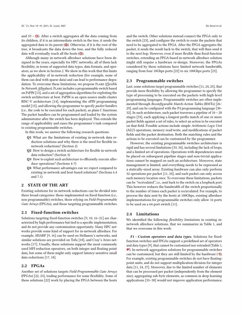
https://doi.org/10.1145/1122445.1122456

https://doi.org/10.1145/1122445.1122456

SC ’21, Nov 14–19, 2021, St. Louis, MO De Sensi et al.

and S3 – B ). After a switch aggregates all the data coming from

its children, if it is an intermediate switch in the tree, it sends the

aggregated data to its parent ( C ). Otherwise, if it is the root of the

tree, it broadcasts the data down the tree, and the fully reduced

data will eventually reach all the hosts (D ).

Although many in-network allreduce solutions have been de-

signed in the years, especially for HPC networks, all of them lack

flexibility, in terms of supported data types, data formats, and oper-

ators, as we show in Section 2. We show in this work that this limits

the applicability of in-network reduction (for example, none of

them can deal with sparse data) and can lead to performance degra-

dation. To overcome these limitations, we propose Flare (FlexibleIn-Network Allreduce). Flare includes a programmable switch based

on PsPIN [13], and a set of aggregation algorithms for exploiting the

switch architecture at best. PsPIN is an open-source multi-cluster

RISC-V architecture [14], implementing the sPIN programming

model [15], and allowing the programmer to specify packet handlers(i.e., the code to be executed for each packet), as plain C functions.

The packet handlers can be programmed and loaded by the system

administrator after the switch has been deployed. This extends the

range of applicability and eases the programmer’s task compared

to existing programmable switches.

In this work, we answer the following research questions:

Q1 What are the limitations of existing in-network data re-

duction solutions and why there is the need for flexible in-

network reductions? (Section 2)

Q2 How to design a switch architecture for flexible in-network

data reduction? (Section 3)

Q3 How to exploit such architecture to efficiently execute allre-

duce operations? (Sections 4-7)

Q4 What performance advantages can we expect compared to

existing in-network and host-based solutions? (Sections 6.4

and 7.1)

2 STATE OF THE ART

Existing solutions for in-network reductions can be divided into

three broad categories: those implemented on fixed-function (i.e.,

non programmable) switches, those relying on Field-ProgrammableGate Arrays (FPGAs), and those targeting programmable switches.

2.1 Fixed-function switches

Solutions targeting fixed-function switches [9, 10, 16–21] are char-

acterized by high performance but tied to a specific implementation,

and do not provide any customization opportunity. Many HPC net-

works provide some kind of support for in-network allreduce. For

example, SHARP [9, 16] can be used on Mellanox’s networks, and

similar solutions are provided on Tofu [18], and Cray’s Aries net-

works [17]. Usually, these solutions support the most commonly

used MPI reduction operators, on both integer and floating point

data, but some of them might only support latency-sensitive small

data reductions [17, 18].

2.2 FPGAs

Another set of solutions targets Field-Programmable Gate Arrays(FPGAs) [22, 23], trading performance for some flexibility. Some of

these solutions [22] work by placing the FPGA between the hosts

and the switch. Other solutions instead connect the FPGA only to

the switch [23], and configure the switch to route the packets that

need to be aggregated to the FPGA. After the FPGA aggregates the

packet, it sends the result back to the switch, that will then send it

to the next hop. However, even if more flexible than fixed-function

switches, extending an FPGA-based in-network allreduce solution

might still require a hardware re-design. Moreover, the FPGAs

considered by these solutions have limited network bandwidth,

ranging from four 10Gbps ports [22] to six 100Gbps ports [23].

2.3 Programmable switches

Last, some solutions target programmable switches [11, 24, 25], that

provide more flexibility by allowing the programmer to specify the

type of processing to be executed on the packets with high-level

programming languages. Programmable switches are often imple-

mented through Reconfigurable Match-Action Tables (RMTs) [26–

29], and can be configured with the P4 programming language [30–

32]. In such architecture, each packet traverses a pipeline of 10− 20

stages [33], each applying a longest-prefix match of one or more

packet fields against a set of rules, to select an action to be executed

on that field. Possible actions include simple Arithmetic Logic Unit(ALU) operations, memory read/write, and modifications of packet

fields and the packet destination. Both the matching rules and the

actions to be executed can be customized by the programmer.

However, the existing programmable switches architecture is

rigid and has several limitations [33, 34], including the lack of loops,

and a limited set of operations. Operations with dependencies must

be placed on subsequent pipeline stages and non-trivial applica-

tions cannot be mapped on such an architecture. Moreover, state

management is limited, and everything needs to be expressed as

a statically-sized array. Existing hardware can also only perform

32 operations per packet [11, 24], and each packet can only access

each memory location once. To overcome these limitations, packets

can be “recirculated”, i.e., sent back to the switch on a loopback port.

This however reduces the bandwidth of the switch proportionally

to the number of times each packet is recirculated. For example, to

process the data sent by the hosts at 100Gbps, existing allreduce

implementations for programmable switches only allow 16 ports

to be used on a 64-port switch [11].

2.4 Limitations

We identified the following flexibility limitations in existing in-

network allreduce solutions, that we summarize in Table 1, and

that we overcome in this work:

F1 - Custom operators and data types. Solutions for fixed-function switches and FPGAs support a predefined set of operators

and data types [9], that cannot be customized nor extended (Table 1,

). In-network aggregation solutions for programmable switches

can be customized, but they are still limited by the hardware ( ).

For example, existing programmable switches do not have floating-

point units, and do not support multiplication/division for integer

data [11, 24, 27]. Moreover, due to the limited number of elements

that can be processed per packet (independently from the element

size), aggregating sub-byte elements, as common in deep learning

applications [35–38] would not improve application performance.

Flare: Flexible In-Network Allreduce SC ’21, Nov 14–19, 2021, St. Louis, MO

On the other hand, Flare provides full customizability of oper-

ators and data types ( ), allowing the user to specify arbitrary

aggregation functions as sPIN handlers (Section 3).

F2 - Sparse data. Many applications need to reduce sparse

data [5, 25, 35, 39], i.e., data containing mostly null values. To save

bandwidth and improve performance, an application might only

transmit and reduce the non-null values. However, to the best

of our knowledge, none of the solutions targeting fixed-function

switches provide explicit support for sparse data ( ). Among the

programmable switches solutions, only one partially targets in-

network sparse data reduction [25]. However, it forces the appli-

cation to sparsify the data per-block, i.e., to send sparse blocks of

dense data ( ). This is however not possible for any application and,

even when possible (for example for deep learning models training),

this negatively affects the convergence of the training [25]. On the

other hand, with Flare we design the first in-network sparse allre-

duce algorithm, that does not make any assumption on the data

sparsity, and can process the data as generated by the hosts ( ),

improving application performance compared to existing solutions

(Section 7.1).

F3 - Reproducibility. Many scientific applications require the

computed results to be reproducible across different runs and for

different allocations. For example, in weather and climate model-

ing, a small difference in computation on the level of a rounding

error could lead to a completely different weather pattern evolu-

tion [40, 41]. However, some aggregation functions (e.g., floating-

point summation [42–46]) might depend on the order in which the

elements are aggregated, and the final result might change if, in

subsequent runs, packets arrive at the switch in a different order.

Many solutions for fixed-function switches ensure reproducibility,

in most cases by storing all the packets and aggregate them in a

pre-defined order only when they are all present [9, 22]. This how-

ever increases the memory occupancy of the switch, even when

this is not required by the application, for example for integer data

or for an application that might tolerate different results across

different runs ( ). Differently from existing solutions, Flare guar-

antees reproducibility only when explicitly requested by the user,

by organizing the aggregation in the switch so that associativity of

the operator is never used. Moreover, Flare reproducible allreduce

does not require storing all the packets before aggregating them

( ).

Fixed-Function Switches FPGAs Progr. Switches

[9] [16] [17] [18] [19] [21] [10] [22] [23] [24] [11] [25] Flare

F1

F2

F3 ? ? ? ?

Table 1: Comparison between existing in-network allreduce

solutions. F1: Custom operators and data types, F2: Sparse

data, F3: Reproducibility. : provided, : partially provided,

: not provided, ?: unknown.

3 SWITCH ARCHITECTURE

Figure 2 illustrates the high-level architecture of a Flare PsPIN-

based programmable switch. After a packet is received from any of

the switch ports, its headers are processed by a parser [47, 48] that,based on configurable matching rules, decides if the packet must

be processed by a processing unit (or sent directly to the routing

tables unit1), and which function must be executed on the packet.

The processing unit can modify the content of each packet, and

decide its destination. We assume that the network administrator

configures the matching rules in the parser through the control

plane [49], specifying the functions to execute for each packet,

based on the values of specific packet fields (e.g., EtherType in the

Ethernet header [50], or IP optional headers). In principle, the code

to be executed could be specified by users of the system, but this

would open security and accountability concerns that are outside

the scope of this paper.

Differently from existing programmable switches [27, 28, 30, 51,

52], that implement the processing unit through ReconfigurableMatch Action (RMT) tables [26, 29], we consider the processing unit

to be implemented as a PsPIN unit [13], highlighted in the right

part of Figure 2. PsPIN is a clustered RISC-V built on top of the

PULP [53] platform. If a packet needs to be processed, the parser

copies the packet in a 4MiB L2 packet memory and sends a request

to a packet scheduler2. The packet scheduler forwards the request

to one of multiple clusters (four in the example). A cluster-local

scheduler (CSCHED) then selects a Handler Processing Units (HPU,eight in the example, denoted with H) where the packet will be

processed, and starts a DMA copy of the packets from the L2 packet

memory to a single-cycle scratchpad 1MiB memory (L1 TCDM -

Tightly-Coupled Data Memory). The cluster scheduler also loads thecode to be executed from the 32KiB L2 programmemory to a cluster-

local 4KiB instruction cache (not shown in the figure). Each HPU

is a RISC-V RI5CY core [54] that can execute sPIN handlers [15]i.e., C functions defining how to process the content of the packet.

The handlers can use the single-cycle L1 memory also to store and

load data, that is preserved after the processing of the packet is

terminated, and until the handler is uninstalled from the control

plane. Each cluster also has a DMA engine that can be used to

access a globally shared 4MiB memory (L2 handler memory).

L2

Packet

Memory

L2

Program

Memory

L2

Handler

Memory

Packet

Scheduler

Command

Unit

Switch

Ports

Crossbar

Parser

Processing

Unit

(PsPIN)

Routing

TablesH

L1 TCDM

DMA

Cluster 0

CSCHED HHH

HH

HH

H

L1 TCDM

DMA

Cluster 1

CSCHED HHH

HH

HH

H

L1 TCDM

DMA

Cluster 3

CSCHED HHH

HH

HH

H

L1 TCDM

DMA

Cluster 2

CSCHED HHH

HH

HH

Figure 2: PsPIN switch high-level architecture.

After processing a packet, each HPU can set its destination and

send it to the routing tables unit through a command unit. After

getting the destination port, the packet is sent to a crossbar unit,

that also implements queueing and quality of service (QoS) func-

tionalities. This unit is also known as traffic manager [27], and

we assume that the implementation and functionalities of both the

routing tables unit and the crossbar are similar to those of any other

switch. When the packet is ready to be sent, it might be processed

1By doing so, packets that do not need additional processing are not further delayed.

2If the packet memory is full, the packet is dropped or congestion is notified before

filling the buffer, depending on the specific network where the switch is integrated.


again by the processing unit3. After this additional and optional

processing step, the packet can be either dropped or forwarded.

The PsPIN processing unit is clocked at 1 GHz, and a PsPIN

unit with four clusters with eight cores each (as the one shown

in the example) occupies 18.5 mm2[13] in a 22nm FDSOI process.

Half of the area in the PsPIN unit is occupied by the L2 memory,

and each cluster occupies on average 2mm2[13], most of which is

L1 memory (1.64mm2). We also add an FP32/FP16 Floating Point

Unit (FPU) [55] to each core, increasing the area of the cluster to

2.29mm2. The processing unit in programmable switches is esti-

mated to occupy up to 140mm2in a 28nm FDSOI process [56]. By

scaling the area, we set a 180mm2target area for our PsPIN unit,

and we then assume we can fit ∼64 clusters and the L2 memory in

our processing unit area budget. We assume that more clusters can

be fit in the unit by organizing them hierarchically (in principle, by

having separate units with a scheduler on the front). Moreover, it

is worth remarking that our estimation of the available area bud-

get is conservative because existing switches are manufactured in

16nm [57] to 7nm [58] processes.

4 FLARE ALLREDUCE GENERAL DESIGN

In Flare, before starting the aggregation, the application sends

a request to a network manager node [9, 16], that computes a

reduction tree, and installs the handlers on all the switches of the

tree through the control plane of the network. For each switch of

the reduction tree, the network manager also sets the number of

ports fromwhich it will receive the packets to be aggregated (i.e., its

children in the reduction tree), and the port to be used to forward

the aggregated data (i.e., the port connected to the parent in the

reduction tree). Because the structure of the reduction tree depends

on the location of the hosts participating in the reduction, this

setup phase must be done once for each subset of hosts executing an

allreduce. For example, in the case ofMPI, this must be done once for

each communicator, similarly to other existing approaches [9, 16].

Each switch can participate simultaneously in different allre-

duces (issued by the same user/application or by different ones), and

the network manager assigns a unique identifier to each allreduce,

so that only packets belonging to the same allreduce are aggregated

together. Because each allreduce consumes some memory resources

on the switch, we assume that the memory is statically partitioned

across a predefined maximum number of allreduces, as done by

most in-network reduction approaches [9, 11, 16–18, 25]. If any

switch on the reduction tree is already managing the maximum

possible number of allreduces, the network manager can try to

recompute a different reduction tree excluding that switch or just

reject the request issued by the application, which then needs to

rely on host-based allreduce [9, 16]. Because the memory is par-

titioned and the compute resources are dynamically assigned, to

simplify the analysis in the following we focus on describing what

happens for a single allreduce.

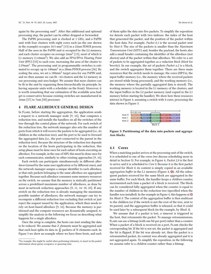
Once the setup is complete, the hosts can start sending the data

to be reduced. We assume that 𝑍 elements must be aggregated and

that each host splits its data in𝑍𝑁

packets of 𝑁 elements each. In

Figure 3 we show an example where we have three hosts, and each

3For example, this might be useful when performing telemetry, to insert in the packet

information about queue occupancy or queueing time.

of them splits the data into five packets. To simplify the exposition

we denote each packet with two indexes: the index of the host

that generated the packet, and the position of the packet within

the host data. For example, Packet 0,1 is the second packet sent

by Host 0. The size of the packets is smaller than the MaximumTransmission Unit (MTU) and, besides the payload, the hosts also

add a small header containing the identifier of the allreduce (not

shown) and of the packet within that allreduce. We refer to a set

of packets to be aggregated together as a reduction block (block for

brevity). In our example, the set of packets Packet x,2 is a block,

and the switch aggregates them together. There are three main

resources that the switch needs to manage: the cores (HPUs), the

input buffer memory (i.e., the memory where the received packets

are stored while being processed), and the working memory (i.e.,

the memory where the partially aggregated data is stored). The

working memory is located in the L1 memory of the clusters, and

the input buffers in the L2 packet memory (and copied in the L1

memory before starting the handler). We show how these resources

interact in Figure 4, assuming a switch with 4 cores, processing the

data shown in Figure 3.

NZ

Host 0 Packet 0,0

Host 1

Host 2

Packet 1,0

Packet 2,0 Packet 2,1

Packet 1,1


Packet 1,2


Packet 1,3


Packet 1,4

Packet 2,4

Block 2

Figure 3: Partitioning of the data into packets and aggrega-tion blocks.

4.1 Cores

When amatching packet arrives at the processing unit of the switch,

it is scheduled to one of the cores (we discuss scheduling more in

detail in Section 5). For example, in Figure 4, Packet 2,0 is the firstto arrive and it is scheduled to Core 0. Because it is the first packetreceived for Block 0, its content is simply copied in an available

aggregation buffer in the L1 memory (Figure 4, A ). All the subse-

quent packets received for the same block are aggregated in the

same buffer. For each block, the handler keeps a children counter,

incremented each time a packet of a block is received. The block

can be considered fully aggregated when the counter is equal to

the number of children in the reduction tree (specified when the

handler was installed). In the example in Figure 4, this happens at B

for Block 0. The content of the aggregation buffer is then multicast

to the children (or if the switch is not the root of the tree, sent to

its parent), and the aggregation buffer is released, so that it could

be used later by a subsequent block (in the example, by Block 3).We assume that if a packet is lost, a timeout is triggered in

the host, that retransmits the packet. To manage retransmissions,

Flare can use a bitmap (with one bit per port) rather than a counter.

When a packet of a block is received on a port, Flare checks the

corresponding bit. If the bit is not set, the packet is aggregated and

the bit is flipped. If the bit was already set, then the packet is a

retransmitted packet, its content was already aggregated and it is

not aggregated again. To simplify the exposition, in the following

we assume refer to a children counter rather than a bitmap.


The aggregation of the packets belonging to the same block can

be done in different ways and has a direct impact on the maximum

bandwidth that can be achieved by the switch when aggregating

data. We denote with 𝜏 the service time of a core (i.e., the num-

ber of cycles it needs to aggregate a packet). Because we have 𝐾

cores (4 in the example), if the workload is evenly distributed across

the cores (and we will show this is the case), the maximum band-

width achievable by the switch is expressed as𝐾𝜏 . We assume the

switch receives a packet every 𝛿 cycles and we can then express

the bandwidth of the switch (in packets processed per cycle) as

ℬ = min

(𝐾𝜏 ,

1

𝛿

). 𝐾 , 𝜏 , and 𝛿 are determined by the specific switch

and network design, and we show in Section 6 how to properly

organize the computation so to minimize 𝜏 .

Chunk 0Block 0

Block 1

Block 3

Time

Cores (HPUs)

and

Input Buffers

Working Memory

A B C

Packet 0,0

Packet 1,0

Packet 1,1

Packet 2,1

Packet 0,1

Packet 2,2

Packet 0,2

Packet 1,2

Packet 1,3

Packet 1,4

Packet 2,3

Core 0

Core 1

Core 3

Core 2

Packet 2,0


Packet 0,4

Block 2

Block 4

Buffer 0

Buffer 1

Buffer 2

τ

δK

ℛ

Figure 4: Utilization of input buffers, cores, and working

memory during an in-network allreduce on a switch with

4 cores, processing the data shown in Figure 3.

4.2 Input Buffers Memory

While being processed, the packets occupy input buffers memory,

for as long as the handler duration. Additionally, if there are no

cores available for scheduling the packet, the packet waits in the

input buffers memory until a core becomes available. In the example

in Figure 4, we denote this situation with a striped pattern in point

C , to indicate that the packet is sitting on a queue waiting to be

scheduled. The input buffer occupancy is thus equal to the time

the packet spends in the queue plus the time it spends while being

processed. We denote the maximum size of these queues with 𝑄 .

For example, Core 0 has𝑄 = 0 at B , and 𝑄 = 1 at C . We model and

analyze this in detail in Section 5.

4.3 Working Memory

We mentioned that the memory is partitioned among multiple

allreduces, and in the example, we assume three buffers have been

allocated to this specific reduction. For simplicity, we also assume

each block is aggregated on a single buffer. However, multiple

concurrent buffers per block could be used, for example, to reduce

contention, and in Section 6 we describe different possibilities for

organizing the working memory. To avoid running out of memory,

each host can have a number of “in-flight” blocks not larger thanthe number of aggregation buffers assigned to that allreduce. In our

example, the hosts send the fourth block only after the first block

has been fully reduced and the buffer has been released. We can

use Little’s Law [59] to determine how many aggregation buffers

should be allocated to each allreduce. Because we have 𝑃 packets

per block (three in this case, equal to the number of hosts), the

target bandwidth (in blocks per cycle), can be simply defined as

ℬ/𝑃 . We define withℒ the latency (in cycles) to process a block

(in our example, the time between A and B in Figure 4), and with

𝑀 the number of buffers needed to aggregate a block. Then, each

allreduce needs a working memory (in number of buffers) equal to

ℛ = 𝑀ℬ

𝑃ℒ.

5 PACKETS SCHEDULING AND INPUT

BUFFERS OCCUPANCY

By default, packets are scheduled to the cores with a First ComeFirst Serve (FCFS) policy, so that they are evenly distributed across

the cores. To simplify the exposition, we also assume that we size

the system so that the interarrival time to the processing unit (i.e.,

the time between the reception of two subsequent packets) is larger

or equal than its service time (i.e., the time between the sending

of two subsequent packets). Under these conditions, on average

packets will never be enqueued because they will always find an

available core. In general, however, packets might be enqueued,

waiting for a core to become available. When the queue is full, the

packet is dropped or congestion is notified before filling the queue,

depending on the specific network where the switch is integrated.

In PsPIN the L1 memory of the switch is partitioned across

multiple clusters of cores (Figure 2). This means that each of the

aggregation buffers shown in Figure 4 is allocated on the L1memory

of a specific cluster. For example, if we assume to have two cores

per cluster, and that Buffer 0 is allocated on the cluster of Cores 0and 1, then the handler running on Core 2 would need to access a

remote L1 memory. By doing so, it incurs a higher latency (up to

25x higher [13]) compared to accessing its local L1 memory.

To only have local L1 accesses and improve performance, we

restrict the processing of packets belonging to the same block to a

subset of cores (located on the same cluster). To keep the workload

balanced among all the available cores, thus still guaranteeing line-

rate processing, we adopt hierarchical FCFS scheduling. We assign

packets belonging to the same block with an FCFS policy to the

same subset of cores, and different blocks to different subsets4. Even

if in the long run this evenly distributes the packets to the cores, it

might generate short bursts of packets directed to the same core(s),

that need to be enqueued, thus increasing the occupancy of the

packets buffers memory. We analyze this more in detail in Section 5.

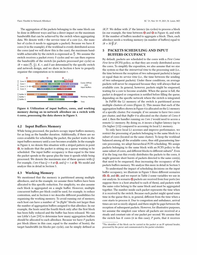
To understand the impact of scheduling decisions on the input

buffer occupancy, we illustrate in Figure 5 three different scenarios

( A , B , and C ), and we report in Table 2 some variables we use in

our analysis. In scenario A packets are received from four ports (we

suppose there is a host attached to each of them), and packets with

the same color belong to the same block and must be aggregated

together. The number inside each packet represents the time when

it is received by the switch. Because each packet might spend some

time in the queue this is, in general, different from the time when a

core starts to process it. Due to congestion and unbalance, arrival

times are not so nicely aligned, and there might be gaps between the

reception of subsequent packets. However, for illustrative purposes,

we assume the simplest case where all packets are received at a

steady and constant rate of one packet per second. We assume that

the switch has 𝐾 cores (4 in this case), 𝑃 ports, that it receives

4The identifier of the block can be carried in the packet as an IP optional header,

processed by the parser and communicated to the packet scheduler.


A1

2

3

0

5

6

7

4

9

10

11

812

13

14

15

S=4

Core 0

Core 3

Core 1

Core 2K=4

Scheduler

Queue

Execution

Time 0 1 2 3 4 5 6 7 8 9 10 11 12 13 14 15

0 0 0 0 1 1 1 1 2 2 2 2 3 3 3 3

3

2 2 3 3 3 3

1 1 1 2 2 2 2 3 3 3 3

τ=4

Q=3

0

4

8

12

1

5

9

13

3

6

10

14

2

7

11

15S=1

Scheduler

B

Core 0

Core 3

Core 1

Core 2K=4

0

1

2

3

4

5

6

7

12

13

14

15

8

9

10

11S=1

SchedulerCore 0

Core 3

Core 1

Core 2K=4C

δk=4

δk=1

4

Queue

Execution

Time 0 1 2 3 4 5 6 7 8 9 10 11 12 13 14 15

0 0 0 0τ=4

4 4 4 8 8 8 8 1212 12 12

0

1

2

3

4

5

6

7

8

9

10

11

12

13

14

15

Port 0

Port 1

Port 2

Port 3

0

1

2

3

4

5

6

7

8

9

10

11

12

13

14

15

Port 0

Port 1

Port 2

Port 3

0

1

2

3

7

4

5

6

10

11

8

9

13

14

15

12

Port 0

Port 1

Port 2

Port 3

4

Queue

Execution

Time 0 1 2 3 4 5 6 7 8 9 10 11 12 13 14 15

0 0 0 0τ=4

4 4 4 8 8 8 8 1212 12 12

Figure 5: Impact of intra-block interarrival time and hierarchical FCFS

scheduling on packets memory occupancy.

Par. Description

𝐾 Number of cores in the switch.

𝑆 Number of cores in each scheduling subset.

𝑃 Number of packets received for each block (this is

equal to the number of children of the switch in

the reduction tree).

𝒬 Maximum number of packets in the switch.

𝛿 Average interarrival time of packets.

𝛿𝑐 Average interarrival time of packets belonging to

the same block.

𝛿𝑘 Average interarrival time of packets to a core (dur-

ing a burst).

𝜏 Average service time of a core.

𝑀 Memory occupied by a block (number of elements).

Table 2: Parameters used in the scheduling mod-

eling.

one packet every 𝛿 seconds (1 in this case), and that each core has

a service time 𝜏 (4 seconds in the example). Because the service

time of the switch is𝜏𝐾

= 𝛿 , if packets are evenly distributed the

switch can process the packets at line rate. We also define 𝛿𝑐 as the

interarrival time of the packetswithin a block (𝛿𝑐 = 1 on scenario A ).

On the right part of the figure we show a detail of what happens in

Core 0. Because it receives a packet every 4 seconds, and its service

time is 4 seconds, packets are never enqueued.

On scenario B of Figure 5, packets belonging to the same block,

are instead assigned to a subset of cores (each containing one core,

i.e., 𝑆 = 1). Each core now does not receive a steady flow of packets,

but bursts of packets at regular intervals. Whereas on scenario A

each core receives one packet every 4 seconds, on scenario B each

core receives 4 packets in 4 seconds, and then nothing for 12 seconds.

Even if in both A and B each core receives on average 4 packets

every 16 seconds, on scenario B the bursts build up queues in front

of each core. On the right part of the figure, we show in detail

what happens in Core 0. The core receives 4 packets in 4 second,

thus building a queue, that will eventually be completely absorbed

before the beginning of the next burst (because we assumed to size

the system to process packets, on average, at line rate). However,

these queues increased the time a packet spent in the switch and,

thus, the input buffer occupancy.

Moreover, the intensity of the bursts (and thus the queue length)

does not only depend on the size of the subsets 𝑆 , but also on 𝛿𝑐 .

For example, in scenario C of Figure 5 we show the same scenario

as B , but now with 𝛿𝑐 = 4, that implies that packets belonging to

the same block will arrive four seconds apart one from on another.

By comparing C with B we can observe that although packets

arrive at the same rate (one packet per second in both cases), and

the scheduler assigns the packets to the same subset of cores, on

scenario C packets of the same block arrive at each core at a slower

rate and are never enqueued, as we can observe in the detail of

Core 0. In this scenario, we obtain the same locality as in scenario

B (packets belonging to the same block are assigned to the same

subset of cores), and the minimal input buffer occupancy as in

scenario A .

𝛿𝑐 depends on non-controllable factors such as application imbal-

ance [60, 61], network noise [62–66], OS noise [67, 68], and network

contention [69–74], but also on some controllable factors, such as

the order the packets are sent by the hosts. In this work, we propose

a solution called staggered sending, that consists in having each host

sending the packets in a different order so that, on average, packets

belonging to the same block can be scheduled to a specific subset

of cores, while not increasing the size of the queues and, thus, the

input buffer occupancy. Moreover, as we show in Section 6.1, stag-gered sending is also helpful in reducing contention on the shared

aggregation buffer. In general, the maximum 𝛿𝑐 we can induce with

staggered sending depends on the number of blocks to be sent. In

the example in scenario C , if we would have only 2 blocks, the 𝛿𝑐would be half of that we have when having 4 blocks. In general, we

have 𝛿 ≤ 𝛿𝑐 ≤ 𝛿 𝑍𝑁.

Input buffer occupancy. Becausewe are considering bursty arrivaltimes at the cores, we can’t use Little’s Law [59] to compute the

average number of packets in the switch, because it would consider

an average case, and would not capture differences between the

three scenarios. Instead, we first compute the interarrival time of

the packets in a burst to a specific core, that we indicate with 𝛿𝑘 .

Packets arrive to a subset of 𝑆 cores with an interarrival time 𝛿𝑐 , and

thus to each of the cores in the subset with interarrival 𝛿𝑘 = 𝑆𝛿𝑐 .

Because we on the long run packers are evenly distributed across

the cores, this can never be higher than 𝐾𝛿 , and thus we have 𝛿𝑘 =

min(𝑆𝛿𝑐 , 𝐾𝛿). Because 𝑃 packets are received for each block, a burst

can contain up to𝑃𝑆packets, and it takes 𝛿𝑘

𝑃𝑆cycles to completely

receive the burst. By that time,𝛿𝑘𝑃𝜏𝑆

packets have been processed by

the core and removed from the queue. Accordingly, we can express

the maximum queue length as𝑄 =𝛿𝑘𝑃𝛿𝑘𝑆

− 𝛿𝑘𝑃𝜏𝑆

= 𝑃𝑆

(1− 𝛿𝑘

𝜏

), and the

maximum number of packets in the switch (including those being

currently processed by each core) as:

𝒬 = (𝑄 + 1)𝐾 =𝑃𝐾

𝑆

(1 − 𝛿𝑘

𝜏

)+ 𝐾 (1)

This equation shows the relationship between the scheduling

decision and the input buffer occupancy (e.g., the smaller 𝑆 , the

higher the input buffer occupancy). It can also be used to compute

the latencyℒ to process a block and, thus, the working memory

occupancy (Section 4.3). Indeed, the latency can be computed as the

time the switch waits for all the packets of the block to be received

((𝑃 −1)𝛿𝑐 ), plus the time needed for processing the last packet. This

includes both the time spent aggregating the packet and the time

spent in the queue. In the worst case, a packet spends 𝑄𝜏 cycles in


the queue, and the latency is equal toℒ = (𝑃 − 1)𝛿𝑐 + (𝑄 + 1)𝜏 . We

use the queueing time and the latency models for estimating the

input buffer and working memory occupancy in Section 6.

6 PARALLELISM AND MEMORY

ORGANIZATION

We now describe the design of different aggregation approaches

that can be used to reduce a block of 𝑃 packets in Flare. We con-

sider different designs: aggregation on a single memory buffer

shared by all the packets of a block (Section 6.1), aggregation on

multiple buffers (Section 6.2), and asynchronous tree aggregation

(Section 6.3). We then analyze the different tradeoffs between these

alternatives in Section 6.4.

When analyzing the different aggregation approaches we model

the service time of a core 𝜏 (Section 4.1). This can then be used to

model the size of the working memory (Section 4.3); and the input

buffer occupancy (Equation 1). To model the working memory size,

we also need to model𝑀 , i.e., the number of buffers used for each

block. In our modeling, we assume to have 1KiB packets contain-

ing 256 floating-point values. We measured the time required to

aggregate a packet in the aggregation buffer by using the PsPIN

cycle-accurate simulator. On average, a core of the PsPIN unit needs

four cycles to sum two 4-bytes floating point values and to store the

result back in the aggregation buffer. Because the unit is clocked at

1GHz (Section 3), the time required to process a packet is 1ns per

byte circa, and we use this information to model 𝜏 .

6.1 Aggregation using a single buffer

The first approach we propose is the most straightforward one,

where all the packets of the same block are accumulated in the

same working memory buffer, as shown in Figure 6. We show on

the left the packets processed by each core, and how the cores

access the buffer. In this case, cores C0, C2, and C3 just sum the

content of their packets into the buffer. Cores C1 also reads back

the fully aggregated result, that will then send on a packet over the

network. On the right, we show the timeline of these operations.

For the cores, the boxes represent the duration of the handlers,

whereas for the buffer we depict for how long the buffer has been

used.

Working

Memory

Cores

B0

+++C0 C1

+C2 C3

B0

Packets P0 P1 P2 P3 Time

C0

C1

C3

C2

B0=P0

B2=P2

B0+=P1

B0

Lτ

B0+=P3

B0+=P2

Figure 6: Single buffer aggregation.

We assume the most general case where the concurrent aggrega-

tion of multiple packets in a shared aggregation buffer is executed

in a critical section. Indeed, even if in principle we could use atomic

operations [75], the computation would still be affected by severe

contention and/or performance overhead [76, 77]. Moreover, by as-

suming a critical section we cover the cases where the user function

cannot be executed by using atomic operations, and the aggregation

of sparse data that, as we will show in Section 7, requires more

complex processing and in most cases needs to be executed anyhow

in a mutually exclusive way.

To avoid expensive context switches, PsPIN handlers are never

suspended and terminate only after the packet has been processed.

Thus, if waiting to enter a critical section, theywill actively consume

compute cycles on one of the cores. For example, when a packet

arrives at C2, the core waits for the buffer to be released by C0 (wedenote this waiting time with a red box), and only then it starts

the aggregation. We define with 𝐿 the number of cycles needed

to aggregate a block after the handler enters the critical section

(i.e., in general, 𝐿 ≤ 𝜏). The probability that two handlers need to

access the same aggregation buffer concurrently depends on 𝛿𝑐 , i.e.,

the interarrival time of the packets belonging to the same block. If

𝛿𝑐 ≥ 𝐿, on average there is never more than one packet of the same

block processed concurrently. This is also true if all the packets of

a block are executed by the same core (i.e., 𝑆 = 1). However, for

𝑆 = 1 the input buffers occupancy would significantly increase, as

discussed in Section 5.

To estimate the cost of contention, we assume to have 𝐶 cores

in each cluster. Because we schedule the packets belonging to the

same block to a subset of 𝐶 cores, in the worst case we have 𝐶

concurrent packets of the same block that need to access the same

aggregation buffer in the working memory. If a handler needs 𝐿

cycles to aggregate the packet (excluding the time spent waiting to

enter the critical section), in the worst case, the first handler to be

executed needs 𝐿 cycles to aggregate the packet, the second handler

2𝐿 cycles, the third handler 3𝐿 cycles, etc. . . In general, the average

service time of a core can thus be expressed as 𝜏 =

∑𝐶𝑖=1 𝑖𝐿

𝐶=𝐿 (𝐶−1)

2.

We then have:

𝜏 ≤{𝐿, 𝑆 = 1 or 𝛿𝑐 ≥ 𝐿.𝐿 (𝐶−1)

2, otherwise.

(2)

We minimize 𝜏 for 𝑆 = 1 or 𝛿𝑐 ≥ 𝐿. As discussed in Section 5, we

can change 𝑆 by restricting the execution of the packets of the same

block to a subset of 𝑆 cores. According to equation 1, by reducing

𝜏 we would decrease the input buffers occupancy. However, this

increase might be canceled out because we are also decreasing

𝑆 . On the other hand, by increasing 𝛿𝑐 we always decrease the

input buffer occupancy, but we increase the latency required for

processing a block and, thus, the working memory occupancy.

Before showing the effect of these decisions on both bandwidth

and memory occupancy, we observe that we can increase 𝛿𝑐 by

using staggered sending, as discussed in Section 5. In a nutshell, this

means that to avoid contention there should never be two cores

working on two packets of the same block. This can only happen if

the data to be reduced is large enough to have, at any time, one block

per core. For our switch, this can only be guaranteed if the hosts use

staggered sending and if the size of the data to be reduced is larger

than 512KiB. Because small-size allreduces are a significant fraction

of the allreduce traffic [2], we propose in the next sections some

alternative approaches to address such cases. Moreover, because

we only need one buffer per block, we have𝑀 = 1.

6.1.1 Main insights. Figure 7 illustrates the modeled bandwidth,

memory occupancy of the input buffers (𝒬), and occupancy of the

working memory (ℛ). On the x-axis, we have different values of 𝑆 .


We consider restricting the execution of packets belonging to the

same block to 1 core, and 𝐶 cores (i.e., all the cores of a cluster).

First, we observe that for small messages (where we can’t suffi-

ciently increase 𝛿𝑐 ) there is a large performance drop when 𝑆 = 𝐶 .

However, having 𝑆 = 1 significantly increases the memory occu-

pancy. For larger messages, we observe good performance also

when scheduling the packets on 𝐶 cores of the same cluster, thus

decreasing the queue length and the occupancy of the input buffers

memory. The occupancy of the working memory is negligible and

around 512KiB. For large enough packets and 𝑆 = 𝐶 , the maximum

total memory occupancy is 2MiB for a single reduction. In general,

scheduling the packets belonging to the same reduction block to a

single core significantly increases the memory occupancy and, for

this reason, in the following we design alternative solutions that

can achieve a higher bandwidth and a lower memory occupancy

for smaller allreduces.

8KiB 64KiB 512KiB0

1

2

3

4

Band

. (Tb

ps)

8KiB 64KiB 512KiB0

10

20

30

Inp.

Buf

f. (M

iB)

8KiB 64KiB 512KiB0.0

0.2

0.4

Wor

k. M

em.

(MiB

)

S=1 S=C

Figure 7: Bandwidth andmemory occupancy of single buffer

aggregation.

6.2 Aggregation on multiple buffers

An extension to the previous aggregation design consists in having

𝐵 aggregation buffers for each block. In Figure 8 we show an exam-

ple with two buffers. When a handler is executed, it takes whichever

of those buffers is not currently used by any other handler. In the

example, differently from the single buffer case, when C2 receivesthe packet, it finds B0 already being used by C0, and thus aggregatesthe packet on B1. If no buffer is available, the handler needs to waitto enter a critical section, as for the single buffer aggregation (for

example, this is what happens to both C1 and C3). Because the ag-gregated data is now distributed over 𝐵 buffers, the last handler to

be executed for the block needs to aggregate together the partially

aggregated data contained in the remaining 𝐵 − 1 buffers. In the

example, the handler running on C1 is the last one to be executed

and, aggregates the content of its packet with the content of B0,and then of B1.

B0

+++C0 C1

+C2 C3

+

B1B0Working

Memory

Cores

Packets P0 P1 P2 P3Time

B0=P0

B2=P2

C0

C1

C3

C2

B0

B1

B1+=P1

B1=P2

B0+=P3 B0+=B1

Figure 8: Multiple buffer aggregation.

𝜏 can be computed starting from Equation 2, by replacing 𝛿𝑐 with

𝐵𝛿𝑐 . Indeed, when using 𝐵 buffers, the probability that two running

handlers need to access the same buffer decreases proportionally

with 𝐵. Compared to the single buffer aggregation, this solution is

less affected by contention for shorter interarrival times (and, thus,

for smaller data). Moreover, the last handler needs to aggregate the

data from the other 𝐵 − 1 buffers, and this costs (𝐵 − 1)𝐿 additional

cycles. Because 𝐵 buffers are stored for each block, we have𝑀 = 𝐵.

6.2.1 Main insights. This aggregation algorithm increases the con-

currency and the bandwidth at the cost of higher memory occu-

pancy. However, using too many buffers reduces the bandwidth,

due to the extra cost required for sequentially aggregating the par-

tially reduced data of each buffer. We analyze the tradeoffs between

bandwidth and memory occupancy in Section 6.4.

6.3 Tree aggregation

Themain drawback of themultiple buffer aggregation, is the sequen-

tial aggregation of the data contained in each of the aggregation

buffers. To avoid that cost, we can organize the computation in a

tree-like way. We illustrate this idea in Figure 9. When a core re-

ceives a packet, it allocates a buffer and copies the data into it. After

copying the data, a core might also aggregate the data contained in

some of the other buffers. The idea is to organize the aggregation

of those buffers in a pre-defined tree-like way. For example, the

data contained in B0 can only be aggregated with B1, and the resultstored back in B1 (after this aggregation step, B0 can be deallocated).Similarly, the data contained in B2 can only be aggregated with B3and stored back in B3 (and B2 deallocated). When B1 contains theresult of B0+B1, and B3 the result of B2+B3, the final aggregation of

B1+B3 can be computed.

Time

B0=P0

B2=P2

B3=P3

B1=P1

Block 4

=C0 C1 C3

B0

+

B3

+

B2B1

+= =C2

=

Working

Memory

Cores

Packets P0 P1 P2 P3

C0

C1

C3

C2

B0

B1

B2

B3

B1+=B0 B1+=B3

B3+=B2

Figure 9: Tree aggregation.

To completely avoid contention on shared aggregation buffers

(independently from 𝛿𝑐 and, thus, from the message size) the com-

putation on the next level of the tree is carried only if a core finds

available data in both buffers. For example, when C0 receives thepacket, it copies it in B0, and could aggregate B0 with B1. However,there is no available data yet in B1, and the handler is terminated.

Instead, when C1 processes its packet, it finds the data in B0 andcarries on the computation of the next level of the tree. It also finds

the result of B2+B3 in B3, and thus also computes B1+B3, and sends

the completely aggregated result on the network. To guarantee

the reproducibility of floating-point summation, a packet coming

from a port 𝑖 is always stored in a buffer 𝑗 . This forces the tree to

always have the same structure and guarantees the reproducibility

of floating-point summation across different runs.

To compute the service time, we assume that the cost of copy-

ing the data is negligible. For example, in PsPIN this can be done

through the DMA engine, at the cost of 64 cycles instead of the 1024

cycles needed for the aggregation. A total of 𝑃 − 1 aggregations are

executed, and we can compute the average number of cycles per


packet as 𝜏 =(𝑃−1)𝐿𝑃

. To compute the memory consumption, we

observe that each time two buffers are aggregated, one of them is

discarded. Because 𝑃 − 1 aggregations are performed and they are

arranged in log 𝑃 levels in the tree, on average we have𝑀 = 𝑃−1log𝑃

active buffers for each block.

6.3.1 Main insights. Differently from single and multiple buffers

aggregation, in this case, the handlers never waste cycles waiting

for entering a critical section, and this design achieves the optimal

bandwidth independently from 𝛿𝑐 and, thus, from the data size.

However, it requires more buffers per block, increasing the aver-

age memory occupancy. We analyze the bandwidth, latency, and

memory occupancy of this design in Section 6.4.

6.4 Evaluation

In Figure 10 we show the modeled maximum bandwidth and the

memory occupancy, for 𝑆 = 𝐶 and different data sizes. We observe

that the only best performing algorithm on data smaller than 128KiB

is the tree aggregation. When increasing the data size, multi-buffers

aggregation catches up, and the higher the number of buffers, the

higher the bandwidth for smaller messages. Eventually, for data

larger than 512KiB, single buffer aggregation catches up with the

other solutions.

64KiB 128KiB 256KiB 512KiBData Size

0

2

4

Band

widt

h (T

bps)

64KiB 128KiB 256KiB 512KiBData Size

0

2

4

Mem

ory

(MiB

)

Single buffer Multi buffers (2) Multi buffers (4) Tree

Figure 10: Modeled bandwidth and memory occupancy for

𝑆 = 𝐶 and different data sizes.

Regarding the memory occupancy, it is worth remarking that, in

some cases, using more buffers decreases the memory occupancy,

because the performance is higher and those buffers are used for

a shorter time. To optimize both compute and memory resources,

Flare uses single buffer aggregation if the size of the data to be

reduced is larger than 512KiB, multi buffers with 4 buffers if larger

than 256KiB, with 2 buffers if larger than 128KiB, and tree aggrega-

tion otherwise. When reproducibility of floating-point summation

is required, Flare always uses tree aggregation.

We implemented the different aggregation algorithms in the

PsPIN cycle-accurate simulator [13]. To simulate delays in the hosts

sending the data and in the network, we generate packets with a

random and exponentially distributed arrival rate. The actual PsPIN

implementation [13] only simulates 4 clusters. Because the clusters

are organized in a shared-nothing configuration, we scale the results

linearly with the number of deployed clusters. First, we report in

Figure 11 the maximum bandwidth that the switch can achieve for

the aggregation of 32-bits integers vectors of different size 𝑍 . We

compare Flare to two baselines: SwitchML [11] and SHARP [9, 16].

SwitchML runs on programmable Tofino switches [27], can only

process integer elements, and achieves a maximum bandwidth of

1.6Tbps [11]. SHARP is a solution running on Mellanox’s fixed-

function switches [78], and can process floating-point elements.

Switches supporting SHARP have 40 ports at 200Gbps. However,

to the best of our knowledge, the best available known data for

SHARP (for a single switch) shows a 3.2Tbps bandwidth [16] (32

ports at 100Gbps), and we use this as a reference.

1KiB 4KiB 512KiB 1MiBData Size

0

1

2

3

Band

wid

th (

Tb

ps) SHARP

SwitchML

int32int16 int8 floatData Type

0

1

2

3

Band

wid

th(E

lem

ents

per

sec) 1e11

SwitchML

Flare (Single Buffer) Flare (Multiple Buffers) Flare (Tree)

Figure 11: Bandwidth for different data size and data types.

We observe that, for small data, only tree aggregation provides

higher bandwidth than SwitchML. Indeed, single and multi-buffers

aggregation cannot exploit staggered sending for small data, and ex-

perience contention when accessing the aggregation buffers. More-

over, for small data, we are showing a “cold start” case, where thehandlers were not loaded yet in the instruction cache. For larger

data, single buffer aggregation efficiently exploits staggered send-

ing, achieving a higher bandwidth compared to multi-buffer and

tree aggregation. Indeed, both multi-buffer and tree aggregation

have some additional overhead caused by the management of mul-

tiple buffers. We also observe that even Flare achieves a higher

bandwidth compared to SwitchML and SHARP, while also capable

of running arbitrary computations on network packets. As we show

in Section 7.1 this leads, for example, to significant performance

improvements when dealing with sparse data.

We also report in Figure 11 the bandwidth (in elements aggre-

gated per second), for different data types, for the aggregation of

1𝑀𝑖𝐵 data. We consider 32-bits, 16-bits, and 8-bits integers, and

floating-point elements (not supported by SwitchML and by exist-

ing programmable switches in general). Programmable switches

can only process a fixed number of elements per packet. Processing

more elements per packet would require more recirculations, thusdecreasing the bandwidth accordingly. On the other hand, in Flare

the HPUs of the PsPIN unit use vectorization and can aggregate,

for example, two int16 elements in a single cycle. This leads to an

increase in the number of elements aggregated per second when

sending elements with a smaller data type. However, differently

from SHARP, Flare currently does not support the aggregation of

double-precision floating-point elements.

7 SPARSE DATA

To reduce the network traffic and increase the performance, ap-

plications dealing with sparse data might send only the non-zero

elements and their positions. In this case, each host splits the data

into blocks so that, on average, each block contains a number of

non-zero elements that would fit in a network packet. This implies

that different hosts might have a different number of elements in

each block, as shown in Figure 12. We show both the partitioning of

the data in reduction blocks and the elements carried by each packet


(packets also carry the position of each element inside the block,

not shown in the figure for the sake of clarity). The number inside

each box represents the value of that specific element. For simplic-

ity, we assume that (due to the MTU) the hosts can send at most

two elements per packet and that the data density (defined as the

average percentage of non-zero elements in each reduction block)

is 50%. Thus, on average, there will be 2 non-zero elements every 4

elements, and thus we set the span of the block to 4 elements.

005031201171000Host 0

920700000406Host 1

Packet 0 Packet 1Block 0 Block 1 Block 21710

46

53

9

121

27

Packet 2

Figure 12: Packetization of sparse data. Packets also carry

the position of the elements (not shown).

However, whereas this is true on average, this introduces the

following additional challenges compared to the dense case:

Multiple blocks per packet. Elements that belongs to two dif-

ferent blocks would be sent in the same packet (like the elements

3 and 5 in Figure 12). This implies that the handler must check,

for each element in the packet, the block it belongs to (to aggregate

it in the correct aggregation buffer), for example by dividing its

index by the number of blocks. This introduces some additional

computation for each element. To avoid this additional overhead,

we send the block identifier in the packet header (as for the dense

case), and we force the hosts to never send multiple blocks in the

same packet, and rather to send a packet even if it is not full (in our

example, a packet with only 3 ).

Block split. Elements belonging to the same block could be split

in two different packets (e.g., elements 7 2 and 9 in Figure 12).

For dense reductions, it was sufficient to keep a children counter,

incremented when a packet was received from a child, and con-

sider the reduction of the block completed when the counter was

equal to the number of children. In the sparse case, a node could

receive multiple packets for the same block, and this approach is

not sufficient anymore. To address this issue each host sends, in

the last packet of a block, a counter representing the number of

packets composing that block. For example, because node 1 splits

block 2 in two packets, it sends the packet carrying element 9 with

the counter set to 2. The handlers keep for each block an additional

shard counter for each of the 𝑃 hosts. The shard counter is incre-

mented every time a packet for that block is received from that port.

When the counter is equal to the value carried in the last packet of

the block, then all the packets for that block and from that specific

port have been received, and the children counter can be increased.

Empty blocks. In some cases, we could have all-zero blocks (for

example, block 1 sent by node 1). In those cases, we still send a

packet with no elements (and with only the header with the iden-

tifier of the block), so that the switch can increase the children

counter nevertheless. If we assume uniformly distributed zero val-

ues, this however should rarely happen.

Another difference compared to the dense case is the design of

the data structure that holds the partially aggregated data. Flare

still aggregates separate blocks in different buffers. However, whereas

for the dense case the aggregation buffer has size 𝑁 , in the sparse

case aggregating two buffers of 𝑁 elements leads, in general, to

more than 𝑁 aggregated elements (because the non-zero elements

in the two buffers might not perfectly overlap). For example, in

Figure 12, aggregating the data in the packet 10 17 with the data in

the packet 6 4 leads to 3 elements ( 6 14 17).

For sparse data, Flare stores the data and the indexes in a hash

table. To avoid expensive collision resolution, when there is a col-

lision, the colliding element is put in a spill buffer. When the spill

buffer is full, the spilled data is immediately sent to the next switch

(or to the hosts). For highly sparse data, this solution reduces mem-

ory consumption compared to storing it in a dense format. For

denser data, this however increases both the memory occupancy

(because indexes must be explicitly stored), the latency when ag-

gregating the data, and the network traffic (because more data

spills).

For denser data, Flare uses a contiguous memory buffer of the

size of the block. From a computational perspective, this is the

design with the lowest latency, because the handler simply needs

to store the element in a specific position. However, when the

reduction is completed, the buffer needs to be entirely scanned and

only the non-zero elements inserted in the packet. Moreover, the

memory consumption will be equal to that of the dense case, thus

much higher than the optimal if the buffer contains many zeros.

In general, sparse data get denser after each aggregation and,

when aggregating data on an in-network reduction tree, the data

get denser while traveling from the hosts to the root of the tree.

For this reason, Flare stores the data in hash tables in the leaves

switches, and in an array in the root switch. The “densification” ofsparse data depends on the number of non-overlapping indexes,

and we analyze these effects at scale in Section 7.1.

We can distribute the computation to the cores using the same

solutions we described in Section 6 for the dense case: single buffer,

multiple buffers, and tree aggregation. We can also use the same

models, with a few caveats. First, for sparse allreduce, the term 𝑃

(i.e., the number of packets expected for a given block) represents

the average case because, as described earlier, each block can be

composed of more or less than 𝑃 packets. Moreover, storing 𝑁

elements might require more than 𝑁 memory cells, depending on

the data structure used to store the partially aggregated data.

7.1 Evaluation

First, we report the modeled bandwidth for both the hash and array

storage in Figure 13, assuming a 10% density. We observe a lower

bandwidth for the sparse allreduce compared to the dense one, due

to the more complex operations that need to be executed by the

handler to store both the indexes and the data. However, as we

will show later, because less data is transmitted, this still allows to

obtain a performance advantage compared to both host-based and

in-network allreduce.

Then, we report the results for a 1MiB allreduce in Figure 14,

analyzing the performance when using both the hash and the array

storage, and for different data density. Deep learning applications

typically sparsify the data by only communicating the top 0.1%

or 1% elements of the original data [39], whereas some graph pro-

cessing algorithms might retain up to 20% of the data [5, 6]. We

observe that, as expected, storing the data as a contiguous array


64KiB 256KiB 512KiBData Size (Sparsified)

0.00.51.01.52.0

Band

widt

h (T

bps) Hash Storage

64KiB 256KiB 512KiBData Size (Sparsified)

0.00.51.01.52.0

Band

widt

h (T

bps) Array Storage

Single buffer Multi buffers (2) Multi buffers (4) Tree

Figure 13: Modeled bandwidth for the Flare sparse allre-

duce.

increases the bandwidth and the memory occupied by each block

compared to using a hash table. We do not report the data about

array storage with 1% density because this requires a 600KiB array

for each block (with, on average, only 6KiB non-zero elements) and

all the concurrently processed blocks do not fit in Flare memory.

Hash table storage is characterized by a constant bandwidth and

memory occupancy independently from the density. Indeed, when

data is stored in a hash table Flare always executes a number of

instructions that only depend on the size of the packet. On the other

hand, for lower density the array storage requires storing a larger

array, thus increasing the number of cycles needed to flush it when

the reduction is over.

20% 10% 1%Density

0

1

2

Band

widt

h (T

bps)

20% 10% 1%Density

0

2

4

6

Bloc

k M

em. (

KiB)

20% 10% 1%Density

0

50

100

Extra

Tra

ffic

(%)

Flare (Sparse - Hash) Flare (Sparse - Array)

Figure 14: Simulated bandwidth, memory per block, and ex-

tra generated traffic for the Flare sparse data allreduce, for

different density and storage types.

However, to avoid costly collision management, with hash stor-

age when there is a collision the element is put in a spill buffer,

that when full is sent over the network. This leads to extra network

traffic, because data is split between the hash table and the spill

buffer, and the switch might not fully aggregate the data. We re-

port the impact of spilling on the network traffic in Figure 14. For

example, we observe that for 20% data density, spilling doubles the

network traffic. On the other hand, array storage never generates

extra traffic, and packets are only sent when the block has been

fully reduced.

To analyze the performance of the Flare sparse allreduce at

scale, we extended the SST simulator [79] so that the switch can

modify in-transit packets, and we implemented both dense and

sparse Flare in-network allreduce, and also the host-based ring

allreduce. Moreover, we also implemented on top of SST the Spar-

CML host-based sparse allreduce [39]. We then tuned the simulator

parameters so that the bandwidth of the switches matches with

that obtained through the cycle-accurate PsPIN simulator. Both the

PsPIN-based simulator and the extended SST simulator are provided

in the artifact.

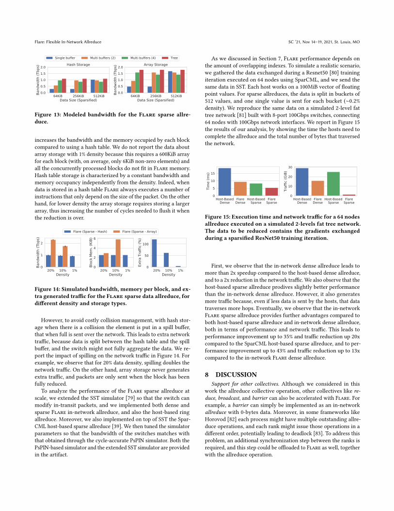
As we discussed in Section 7, Flare performance depends on

the amount of overlapping indexes. To simulate a realistic scenario,

we gathered the data exchanged during a Resnet50 [80] training

iteration executed on 64 nodes using SparCML, and we send the

same data in SST. Each host works on a 100MiB vector of floating

point values. For sparse allreduces, the data is split in buckets of

512 values, and one single value is sent for each bucket (∼0.2%density). We reproduce the same data on a simulated 2-level fat

tree network [81] built with 8-port 100Gbps switches, connecting

64 nodes with 100Gbps network interfaces. We report in Figure 15

the results of our analysis, by showing the time the hosts need to

complete the allreduce and the total number of bytes that traversed

the network.

Host-BasedDense

FlareDense

Host-BasedSparse

FlareSparse

0

5

10

15

Tim

e (m

s)

Host-BasedDense

FlareDense

Host-BasedSparse

FlareSparse

0

10

20

30

Traf

fic (G

iB)

Figure 15: Execution time and network traffic for a 64 nodes

allreduce executed on a simulated 2-levels fat tree network.

The data to be reduced contains the gradients exchanged

during a sparsified ResNet50 training iteration.

First, we observe that the in-network dense allreduce leads to

more than 2x speedup compared to the host-based dense allreduce,

and to a 2x reduction in the network traffic.We also observe that the

host-based sparse allreduce prodives slightly better performance

than the in-network dense allreduce. However, it also generates

more traffic because, even if less data is sent by the hosts, that data

traverses more hops. Eventually, we observe that the in-network

Flare sparse allreduce provides further advantages compared to

both host-based sparse allreduce and in-network dense allreduce,

both in terms of performance and network traffic. This leads to

performance improvement up to 35% and traffic reduction up 20x

compared to the SparCML host-based sparse allreduce, and to per-

formance improvement up to 43% and traffic reduction up to 13x

compared to the in-network Flare dense allreduce.

8 DISCUSSION

Support for other collectives. Although we considered in this

work the allreduce collective operation, other collectives like re-duce, broadcast, and barrier can also be accelerated with Flare. For

example, a barrier can simply be implemented as an in-network

allreduce with 0-bytes data. Moreover, in some frameworks like

Horovod [82] each process might have multiple outstanding allre-

duce operations, and each rank might issue those operations in a

different order, potentially leading to deadlock [83]. To address this

problem, an additional synchronization step between the ranks is

required, and this step could be offloaded to Flare as well, together

with the allreduce operation.


Limitations. As we shown in Section 7.1, the bandwidth achievedby the in-network sparse allreduce is lower than its dense counter-

part, due to the higher latency required for processing and aggre-

gating the sparse data. In our experiments, the lower bandwidth

was compensated by the reduction in the amount of processed data,

and the Flare in-network sparse allreduce outperformed the Spar-

CML host-based sparse allreduce. However, we believe that there is

still space for improvement, either by optimizing the handlers code

or by introducing hardware support to optimize indirect memory

accesses [84].

9 CONCLUSIONS

In this work, we introduced Flare, an architecture for flexible in-

network data reduction. Flare is based on the open-source PsPIN

RISC-V architecture, and allows running custom packet processing

handlers on network packets. Flare also includes a set of aggre-

gation algorithms with different performance and memory occu-

pancy tradeoffs. We modeled and analyzed in detail each of these

algorithms, in terms of bandwidth and memory occupancy. We

then implemented the aggregation algorithms in the PsPIN cycle-

accurate simulator, and analyzed their performance for different

allreduce sizes and datatypes, comparing them with state-of-the-art

in-network aggregation approaches such as SHARP and SwitchML.

Moreover, we also designed and implemented the first (to the best of

our knowledge) in-network sparse allreduce algorithm. We imple-

mented the algorithm in the PsPIN and SST simulators, showing per-

formance improvements and network traffic reduction compared

to in-network dense allreduce and host-based sparse allreduce.

ACKNOWLEDGMENTS

This work has been partially funded by the EPIGRAM-HS project

under grant agreement no. 801039, and the European Project RED-

SEA under grant agreement no. 955776. Daniele De Sensi is sup-

ported by an ETH Postdoctoral Fellowship (19-2 FEL-50).

REFERENCES

[1] Message Passing Forum. Mpi: A message-passing interface standard. Technical

report, USA, 1994.

[2] Sudheer Chunduri, Scott Parker, Pavan Balaji, Kevin Harms, and Kalyan Kumaran.

Characterization of mpi usage on a production supercomputer. In Proceedings ofthe International Conference for High Performance Computing, Networking, Storage,and Analysis, SC ’18. IEEE Press, 2018.

[3] Steven Gottlieb, W. Liu, William D Toussaint, R. L. Renken, and R. L. Sugar.

Hybrid-molecular-dynamics algorithms for the numerical simulation of quantum

chromodynamics. Physical review D: Particles and fields, 35(8):2531–2542, 1987.[4] Tal Ben-Nun and Torsten Hoefler. Demystifying parallel and distributed deep

learning: An in-depth concurrency analysis. ACM Comput. Surv., 52(4), August2019.

[5] H. Zhao and J. Canny. Kylix: A sparse allreduce for commodity clusters. In 201443rd International Conference on Parallel Processing, pages 273–282, 2014.

[6] Huasha Zhao and John F. Canny. Sparse allreduce: Efficient scalable communica-

tion for power-law data. CoRR, abs/1312.3020, 2013.[7] Torsten Hoefler, Andrew Lumsdaine, and Jack Dongarra. Towards efficient

mapreduce using mpi. In Matti Ropo, Jan Westerholm, and Jack Dongarra,

editors, Recent Advances in Parallel Virtual Machine and Message Passing Interface,pages 240–249, Berlin, Heidelberg, 2009. Springer Berlin Heidelberg.

[8] Pitch Patarasuk and Xin Yuan. Bandwidth optimal all-reduce algorithms for

clusters of workstations. Journal of Parallel and Distributed Computing, 69(2):117– 124, 2009.

[9] Richard L. Graham, Devendar Bureddy, Pak Lui, Hal Rosenstock, Gilad Shainer,

Gil Bloch, Dror Goldenerg, Mike Dubman, Sasha Kotchubievsky, Vladimir Koush-

nir, Lion Levi, Alex Margolin, Tamir Ronen, Alexander Shpiner, Oded Wertheim,

and Eitan Zahavi. Scalable Hierarchical Aggregation Protocol (SHArP): A Hard-

ware Architecture for Efficient Data Reduction. In Proceedings of COM-HPC 2016:

1st Workshop on Optimization of Communication in HPC Runtime Systems - Heldin conjunction with SC 2016: The International Conference for High PerformanceComputing, Networking, Storage and Analysis, pages 1–10. Institute of Electricaland Electronics Engineers Inc., jan 2017.

[10] Benjamin Klenk, Nan Jiang, Greg Thorson, and Larry Dennison. An in-network

architecture for accelerating shared-memory multiprocessor collectives. In Pro-ceedings of the ACM/IEEE 47th Annual International Symposium on ComputerArchitecture, ISCA ’20, page 996–1009. IEEE Press, 2020.

[11] Amedeo Sapio, Marco Canini, Chen-Yu Ho, Jacob Nelson, Panos Kalnis,

Changhoon Kim, Arvind Krishnamurthy, Masoud Moshref, Dan R. K. Ports, and

Peter Richtárik. Scaling distributed machine learning with in-network aggrega-

tion. In 18th USENIX Symposium on Networked Systems Design and Implementation(NSDI 21). USENIX Association, April 2021.

[12] Dennis Abts, Michael R. Marty, Philip M. Wells, Peter Klausler, and Hong Liu.

Energy proportional datacenter networks. SIGARCH Comput. Archit. News,38(3):338–347, June 2010.

[13] Salvatore Di Girolamo, Andreas Kurth, Alexandru Calotoiu, Thomas Benz, Timo

Schneider, Jakub Beranek, Luca Benini, and Torsten Hoefler. A risc-v in-network

accelerator for flexible high-performance low-power packet processing. In 2021ACM/IEEE 48th Annual International Symposium on Computer Architecture (ISCA),2021.

[14] Andrew Waterman, Yunsup Lee, David A. Patterson, and Krste Asanović. The

risc-v instruction set manual, volume i: User-level isa, version 2.0. Technical

Report UCB/EECS-2014-54, EECS Department, University of California, Berkeley,

May 2014.

[15] Torsten Hoefler, Salvatore Di Girolamo, Konstantin Taranov, Ryan E. Grant, and

Ron Brightwell. Spin: High-performance streaming processing in the network.

In Proceedings of the International Conference for High Performance Computing,Networking, Storage and Analysis, SC ’17, New York, NY, USA, 2017. Association

for Computing Machinery.

[16] Richard L. Graham, Lion Levi, Devendar Burredy, Gil Bloch, Gilad Shainer, David

Cho, George Elias, Daniel Klein, Joshua Ladd, Ophir Maor, Ami Marelli, Valentin

Petrov, Evyatar Romlet, Yong Qin, and Ido Zemah. Scalable Hierarchical Aggre-

gation and Reduction Protocol (SHARP)TM Streaming-Aggregation Hardware

Design and Evaluation. In Lecture Notes in Computer Science (including subseriesLecture Notes in Artificial Intelligence and Lecture Notes in Bioinformatics), volume

12151 LNCS, pages 41–59. Springer, jun 2020.

[17] Bob Alverson, Edwin Froese, Larry Kaplan, and Duncan Roweth. Cray xc series

network. Cray Inc., White Paper WP-Aries01-1112, 2012.[18] Y. Ajima, T. Kawashima, T. Okamoto, N. Shida, K. Hirai, T. Shimizu, S. Hiramoto,

Y. Ikeda, T. Yoshikawa, K. Uchida, and T. Inoue. The tofu interconnect d. In 2018IEEE International Conference on Cluster Computing (CLUSTER), pages 646–654,2018.

[19] B. Arimilli, R. Arimilli, V. Chung, S. Clark, W. Denzel, B. Drerup, T. Hoefler,

J. Joyner, J. Lewis, J. Li, N. Ni, and R. Rajamony. The percs high-performance

interconnect. In 2010 18th IEEE Symposium on High Performance Interconnects,pages 75–82, 2010.

[20] B. Arimilli, Bernard C. Drerup, Paul F. Lecocq, and Hanhong Xue. Collective

acceleration unit tree structure, U.S. Patent US8756270B2, 17/06/2014.

[21] J. P. Grossman, B. Towles, B. Greskamp, and D. E. Shaw. Filtering, reductions

and synchronization in the anton 2 network. In 2015 IEEE International Paralleland Distributed Processing Symposium, pages 860–870, 2015.

[22] Nadeen Gebara, Paolo Costa, and Manya Ghobadi. Panama: In-network aggrega-

tion for shared machine learning clusters. In Conference on Machine Learningand Systems (MLSys), April 2021.

[23] Shuo Liu, Qiaoling Wang, Junyi Zhang, Qinliang Lin, Yao Liu, Meng Xu, Ray C. C.

Chueng, and Jianfei He. Netreduce: Rdma-compatible in-network reduction for

distributed dnn training acceleration, 2020.

[24] ChonLam Lao, Yanfang Le, Kshiteej Mahajan, Yixi Chen, Wenfei Wu, Aditya

Akella, andMichael Swift. ATP: In-network aggregation for multi-tenant learning.

In 18th USENIX Symposium on Networked Systems Design and Implementation(NSDI 21). USENIX Association, April 2021.

[25] Jiawei Fei, Chen-Yu Ho, Atal Narayan Sahu, Marco Canini, and Amedeo Sapio.

Efficient Sparse Collective Communication and its application to Accelerate

Distributed Deep Learning. Technical report, KAUST, Sep 2020.

[26] Pat Bosshart, Glen Gibb, Hun-Seok Kim, George Varghese, NickMcKeown,Martin

Izzard, Fernando Mujica, and Mark Horowitz. Forwarding metamorphosis: Fast

programmable match-action processing in hardware for sdn. SIGCOMM Comput.Commun. Rev., 43(4):99–110, August 2013.

[27] Intel. Intel Tofino Series. https://www.intel.com/content/www/us/en/products/

network-io/programmable-ethernet-switch.html, mar 2021.

[28] Recep Ozdag Intel. Intel (R) Ethernet Switch FM6000 Series – Software Defined

Networking. https://people.ucsc.edu/ warner/Bufs/ethernet-switch-fm6000-sdn-

paper.pdf, mar 2021.

[29] R. Bifulco and G. Rétvári. A survey on the programmable data plane: Abstractions,

architectures, and open problems. In 2018 IEEE 19th International Conference onHigh Performance Switching and Routing (HPSR), pages 1–7, 2018.

https://www.intel.com/content/www/us/en/products/network-io/programmable-ethernet-switch.html

https://www.intel.com/content/www/us/en/products/network-io/programmable-ethernet-switch.html


[30] Pat Bosshart, Dan Daly, Glen Gibb, Martin Izzard, Nick McKeown, Jennifer Rex-

ford, Cole Schlesinger, Dan Talayco, Amin Vahdat, George Varghese, and David

Walker. P4: Programming protocol-independent packet processors. SIGCOMMComput. Commun. Rev., 44(3):87–95, July 2014.

[31] Frederik Hauser, Marco Häberle, Daniel Merling, Steffen Lindner, Vladimir Gure-

vich, Florian Zeiger, Reinhard Frank, and Michael Menth. A survey on data plane

programming with p4: Fundamentals, advances, and applied research, 2021.

[32] Elie F. Kfoury, Jorge Crichigno, and Elias Bou-Harb. An exhaustive survey on

p4 programmable data plane switches: Taxonomy, applications, challenges, and

future trends, 2021.

[33] Dan R. K. Ports and Jacob Nelson. When should the network be the computer?

In Proceedings of the Workshop on Hot Topics in Operating Systems, HotOS ’19,

page 209–215, New York, NY, USA, 2019. Association for Computing Machinery.

[34] Naveen Kr. Sharma, Antoine Kaufmann, Thomas Anderson, Arvind Krishna-

murthy, Jacob Nelson, and Simon Peter. Evaluating the power of flexible packet

processing for network resource allocation. In 14th USENIX Symposium on Net-worked Systems Design and Implementation (NSDI 17), pages 67–82, Boston, MA,

March 2017. USENIX Association.

[35] Torsten Hoefler, Dan Alistarh, Tal Ben-Nun, Nikoli Dryden, and Alexandra Peste.

Sparsity in deep learning: Pruning and growth for efficient inference and training

in neural networks, 2021.

[36] Song Han, Huizi Mao, and William J. Dally. Deep compression: Compressing

deep neural networks with pruning, trained quantization and huffman coding,

2016.

[37] Nikoli Dryden, SamAde Jacobs, TimMoon, and Brian Van Essen. Communication

quantization for data-parallel training of deep neural networks. In Proceedings ofthe Workshop on Machine Learning in High Performance Computing Environments,MLHPC ’16, page 1–8. IEEE Press, 2016.

[38] Vincent Vanhoucke, Andrew Senior, and Mark Z. Mao. Improving the speed of

neural networks on cpus. In Deep Learning and Unsupervised Feature LearningWorkshop, NIPS 2011, 2011.

[39] Cedric Renggli, Saleh Ashkboos, Mehdi Aghagolzadeh, Dan Alistarh, and Torsten

Hoefler. Sparcml: High-performance sparse communication for machine learning.

In Proceedings of the International Conference for High Performance Computing,Networking, Storage and Analysis, SC ’19, New York, NY, USA, 2019. Association

for Computing Machinery.

[40] Christoph Schär, Oliver Fuhrer, Andrea Arteaga, Nikolina Ban, Christophe

Charpilloz, Salvatore Di Girolamo, Laureline Hentgen, Torsten Hoefler, Xavier

Lapillonne, David Leutwyler, Katherine Osterried, Davide Panosetti, Stefan Rüdis-

ühli, Linda Schlemmer, Thomas Schulthess, Michael Sprenger, Stefano Ubbiali,

and Heini Wernli. Kilometer-scale climate models: Prospects and challenges.

Bulletin of the American Meteorological Society, 100(12), Dec. 2019. Early Online

Release.

[41] Edward N. Lorenz. The predictability of a flow which possesses many scales of

motion. Tellus, 21(3):289–307, 1969.[42] Beate Geyer, Thomas Ludwig, and Hans von Storch. Limits of reproducibility

and hydrodynamic noise in atmospheric regional modelling. CommunicationsEarth & Environment, 2(1):17, Jan 2021.

[43] Sylvain Collange, David Defour, Stef Graillat, and Roman Iakymchuk. Numerical

reproducibility for the parallel reduction on multi- and many-core architectures.

Parallel Computing, 49:83–97, 2015.[44] P. Balaji and D. Kimpe. On the reproducibility of mpi reduction operations. In

2013 IEEE 10th International Conference on High Performance Computing andCommunications 2013 IEEE International Conference on Embedded and UbiquitousComputing, pages 407–414, 2013.

[45] N. Revol and P. Theveny. Numerical reproducibility and parallel computations:

Issues for interval algorithms. IEEE Transactions on Computers, 63(08):1915–1924,aug 2014.

[46] Oreste Villa, Vidhya Gurumoorthi, and Sriram Krishnamoorthy. Effects of

floating-point nonassociativity on numerical computations on massively multi-

threaded systems. In In CUG 2009 Proceedings, pages 1–11, 2009.[47] Hesam Zolfaghari, Davide Rossi, and Jari Nurmi. A custom processor for protocol-

independent packet parsing. Microprocessors and Microsystems, 72:102910, 2020.[48] G. Gibb, G. Varghese, M. Horowitz, and N. McKeown. Design principles for

packet parsers. In Architectures for Networking and Communications Systems,pages 13–24, 2013.

[49] Nick Feamster, Jennifer Rexford, and Ellen Zegura. The road to sdn: An intel-

lectual history of programmable networks. SIGCOMM Comput. Commun. Rev.,44(2):87–98, April 2014.

[50] Internet Control Message Protocol. RFC 894, April 1984.

[51] Anirudh Sivaraman, Alvin Cheung, Mihai Budiu, Changhoon Kim, Mohammad

Alizadeh, Hari Balakrishnan, George Varghese, Nick McKeown, and Steve Lick-

ing. Packet transactions: High-level programming for line-rate switches. In

Proceedings of the 2016 ACM SIGCOMM Conference, SIGCOMM ’16, page 15–28,

New York, NY, USA, 2016. Association for Computing Machinery.

[52] Salvatore Pontarelli, Roberto Bifulco, Marco Bonola, Carmelo Cascone, Marco

Spaziani, Valerio Bruschi, Davide Sanvito, Giuseppe Siracusano, Antonio Capone,

Michio Honda, Felipe Huici, and Giuseppe Siracusano. Flowblaze: Stateful packet

processing in hardware. In 16th USENIX Symposium on Networked SystemsDesign and Implementation (NSDI 19), pages 531–548, Boston, MA, February 2019.

USENIX Association.

[53] Davide Rossi, Francesco Conti, Andrea Marongiu, Antonio Pullini, Igor Loi,

Michael Gautschi, Giuseppe Tagliavini, Alessandro Capotondi, Philippe Flatresse,

and Luca Benini. PULP: A parallel ultra low power platform for next generation

IoT applications. In 2015 IEEE Hot Chips 27 Symposium (HCS), pages 1–39. IEEE,2015.

[54] M. Gautschi, P. D. Schiavone, A. Traber, I. Loi, A. Pullini, D. Rossi, E. Flamand,

F. K. Gürkaynak, and L. Benini. Near-threshold risc-v core with dsp extensions

for scalable iot endpoint devices. IEEE Transactions on Very Large Scale Integration(VLSI) Systems, 25(10):2700–2713, 2017.

[55] S. Mach, F. Schuiki, F. Zaruba, and L. Benini. Fpnew: An open-source multi-

format floating-point unit architecture for energy-proportional transprecision

computing. IEEE Transactions on Very Large Scale Integration (VLSI) Systems,29(04):774–787, apr 2021.

[56] H. Zolfaghari, D. Rossi, W. Cerroni, H. Okuhara, C. Raffaelli, and J. Nurmi. Flexi-

ble software-defined packet processing using low-area hardware. IEEE Access,8:98929–98945, 2020.

[57] Daniele De Sensi, Salvatore Di Girolamo, Kim H. McMahon, Duncan Roweth,

and Torsten Hoefler. An in-depth analysis of the slingshot interconnect. In

Proceedings of the International Conference for High Performance Computing,Networking, Storage and Analysis, SC ’20. IEEE Press, 2020.

[58] Broadcom. Tomahawk4 BCM56990 Series.

https://www.broadcom.com/products/ethernet-

connectivity/switching/strataxgs/bcm56990-series, mar 2019.

[59] John D. C. Little. A Proof for the Queuing Formula: 𝐿 = _𝑊 . Oper. Res.,9(3):383–387, June 1961.

[60] Shigang Li, Tal Ben-Nun, Salvatore Di Girolamo, Dan Alistarh, and Torsten

Hoefler. Taming unbalanced training workloads in deep learning with partial

collective operations. In Proceedings of the 25th ACM SIGPLAN Symposium onPrinciples and Practice of Parallel Programming, pages 45–61, 2020.

[61] Ahmad Faraj, Pitch Patarasuk, and Xin Yuan. A study of process arrival patterns

for mpi collective operations. Int. J. Parallel Program., 36(6):543–570, December

2008.

[62] Daniele De Sensi, Salvatore Di Girolamo, and Torsten Hoefler. Mitigating network

noise on dragonfly networks through application-aware routing. In Proceedings ofthe International Conference for High Performance Computing, Networking, Storageand Analysis, SC ’19, New York, NY, USA, 2019. Association for Computing

Machinery.

[63] T. Groves, Y. Gu, and N. J. Wright. Understanding performance variability on

the aries dragonfly network. In 2017 IEEE International Conference on ClusterComputing (CLUSTER), pages 809–813, Sept 2017.

[64] T. Hoefler, T. Schneider, and A. Lumsdaine. The impact of network noise at

large-scale communication performance. In 2009 IEEE International Symposiumon Parallel Distributed Processing, pages 1–8, May 2009.

[65] Sudheer Chunduri, Kevin Harms, Scott Parker, Vitali Morozov, Samuel Oshin,

Naveen Cherukuri, and Kalyan Kumaran. Run-to-run variability on xeon phi

based cray xc systems. In Proceedings of the International Conference for HighPerformance Computing, Networking, Storage and Analysis, SC ’17, pages 52:1–

52:13, New York, NY, USA, 2017. ACM.

[66] D. Skinner and W. Kramer. Understanding the causes of performance variability

in hpc workloads. In IEEE International. 2005 Proceedings of the IEEE WorkloadCharacterization Symposium, 2005., pages 137–149, Oct 2005.

[67] Torsten Hoefler, Timo Schneider, and Andrew Lumsdaine. Characterizing the

influence of system noise on large-scale applications by simulation. In Proceedingsof the 2010 ACM/IEEE International Conference for High Performance Computing,Networking, Storage and Analysis, SC ’10, pages 1–11, Washington, DC, USA,

2010. IEEE Computer Society.

[68] A. Morari, R. Gioiosa, R. W. Wisniewski, F. J. Cazorla, and M. Valero. A quantita-

tive analysis of os noise. In 2011 IEEE International Parallel Distributed ProcessingSymposium, pages 852–863, 2011.

[69] Bogdan Prisacari, German Rodriguez, Philip Heidelberger, Dong Chen, Cyriel

Minkenberg, and Torsten Hoefler. Efficient task placement and routing of nearest

neighbor exchanges in dragonfly networks. In Proceedings of the 23rd InternationalSymposium on High-performance Parallel and Distributed Computing, HPDC ’14,

pages 129–140, New York, NY, USA, 2014. ACM.

[70] Samuel D. Pollard, Nikhil Jain, Stephen Herbein, and Abhinav Bhatele. Evaluation

of an interference-free node allocation policy on fat-tree clusters. In Proceedingsof the International Conference for High Performance Computing, Networking,Storage, and Analysis, SC ’18, pages 26:1–26:13, Piscataway, NJ, USA, 2018. IEEE

Press.

[71] Abhinav Bhatele and Laxmikant V. Kalé. Quantifying network contention on

large parallel machines. Parallel Processing Letters, 19(04):553–572, 2009.[72] X. Yang, J. Jenkins, M. Mubarak, R. B. Ross, and Z. Lan. Watch out for the

bully! job interference study on dragonfly network. In SC ’16: Proceedings of theInternational Conference for High Performance Computing, Networking, Storageand Analysis, pages 750–760, Nov 2016.


[73] X.Wang, M.Mubarak, X. Yang, R. B. Ross, and Z. Lan. Trade-off study of localizing

communication and balancing network traffic on a dragonfly system. In 2018IEEE International Parallel and Distributed Processing Symposium (IPDPS), pages1113–1122, May 2018.

[74] Staci A. Smith, Clara E. Cromey, David K. Lowenthal, Jens Domke, Nikhil Jain,

Jayaraman J. Thiagarajan, and Abhinav Bhatele. Mitigating inter-job interference

using adaptive flow-aware routing. In Proceedings of the International Conferencefor High Performance Computing, Networking, Storage and Analysis, SC ’18, 2018.

[75] A. Kurth, S. Riedel, F. Zaruba, T. Hoefler, and L. Benini. Atuns: Modular and

scalable support for atomic operations in a shared memory multiprocessor. In

2020 57th ACM/IEEE Design Automation Conference (DAC), pages 1–6, 2020.[76] H. Schweizer, M. Besta, and T. Hoefler. Evaluating the cost of atomic operations

on modern architectures. In 2015 International Conference on Parallel Architectureand Compilation (PACT), pages 445–456, 2015.

[77] Maciej Besta and Torsten Hoefler. Accelerating irregular computations with

hardware transactional memory and active messages. In Proceedings of the 24thInternational Symposium on High-Performance Parallel and Distributed Computing,HPDC ’15, page 161–172, New York, NY, USA, 2015. Association for Computing

Machinery.

[78] Mellanox. Mellanox Quantum Switches. https://www.mellanox.com/products/

infiniband-switches-ic/quantum, mar 2019.

[79] A. F. Rodrigues, K. S. Hemmert, B. W. Barrett, C. Kersey, R. Oldfield, M. Weston,

R. Risen, J. Cook, P. Rosenfeld, E. Cooper-Balis, and B. Jacob. The structural

simulation toolkit. SIGMETRICS Perform. Eval. Rev., 38(4):37–42, March 2011.

[80] Kaiming He, Xiangyu Zhang, Shaoqing Ren, and Jian Sun. Deep residual learning

for image recognition. In 2016 IEEE Conference on Computer Vision and PatternRecognition (CVPR), pages 770–778, 2016.

[81] C. E. Leiserson. Fat-trees: Universal networks for hardware-efficient supercom-

puting. IEEE Transactions on Computers, C-34(10):892–901, 1985.[82] Alexander Sergeev and Mike Del Balso. Horovod: fast and easy distributed deep

learning in tensorflow, 2018.

[83] Thorsten Kurth, Sean Treichler, Joshua Romero, Mayur Mudigonda, Nathan

Luehr, Everett Phillips, Ankur Mahesh, Michael Matheson, Jack Deslippe, Massi-

miliano Fatica, Prabhat, and Michael Houston. Exascale deep learning for climate

analytics. In Proceedings of the International Conference for High PerformanceComputing, Networking, Storage, and Analysis, SC ’18. IEEE Press, 2018.

[84] Paul Scheffler, Florian Zaruba, Fabian Schuiki, Torsten Hoefler, and Luca Benini.

Indirection Stream Semantic Register Architecture for Efficient Sparse-Dense

Linear Algebra. 2021.

https://www.mellanox.com/products/infiniband-switches-ic/quantum

https://www.mellanox.com/products/infiniband-switches-ic/quantum

flare: flexible in-network allreduce

Documents