five facts about shale: it’s coming back, and coming back strong

Please see important disclaimer and disclosures at the end of the document

COMMODITIES

7 February 2017

Important Notice: The circumstances in which this publication has been produced are such that it is not appropriate to characterise it as independent

investment research as referred to in MiFID and that it should be treated as a marketing communication even if it contains a research recommendation.

This publication is also not subject to any prohibition on dealing ahead of the dissemination of investment research. However, SG is required to have

policies to manage the conflicts which may arise in the production of its research, including preventing dealing ahead of investment research.

Commodity Compass

Five facts about shale: it’s coming back, and coming back strong

With oil prices back above the psychological $50 threshold and the OPEC/non-OPEC

agreement on the table, the market is very much focused on its compliance. Attention is

also inevitably drawn to the dynamics of US shale production. Will the US recovery

offset OPEC cuts? Accordingly, we review some of the key dynamics of US shale

production. Specifically, we highlight 5 facts about US shale production that all point to

the same underlying trend: US shale is coming back, and it’s coming back strong.

1. Rig counts are increasing at an accelerating pace, and given the technological

advances of the past 3 years, this should translate into significant supply.

2. Decline rates for US shale wells are still steep, but initial production levels,

production profiles, and ultimate recovery volumes have increased. Going

forward, higher production profiles mean stronger aggregate supply.

3. Preliminary US EIA estimates indicate that net new shale supply turned positive

in December, the first time since March 2015. Net new supply recovered just 7

months after rig counts bottomed out and began to increase.

4. The increase of drilling activity comes on the back of a large stock of drilled

and uncompleted wells (DUCs). The industry is also vigorously adding to this

stock, which demonstrates that the shale sector is again recovering/expanding.

5. Evidence from the Bureau of Labor Statistics (BLS) is showing the oil and gas

labor market is stabilizing and reversing its declining trend.

Figure 1.1 – The SG NEW Overbought/Oversold Indicator. Commodities in the oversold (red) box are vulnerable to short-covering

and commodities in the overbought (blue) box vulnerable to profit-taking.

The SG OBOS indicator defines and identifies “oversold” (“overbought”) commodities on a weekly basis as those that are lying at the intersection of extremes in

both short (long) positioning and price weakness (strength). The “oversold” (“overbought”) box is shown in red (blue) in Figure 1.1. Commodities within the

“oversold” (“overbought”) box are trading in the bottom (top) 25% of their price range and have a short (long) position (calculated as the short [long] Money

Manager [MM] open interest [OI] as a percentage of total OI [source: CFTC COT report]) in excess of 75% of the historical maximum. These commodities are

vulnerable to short-covering (profit-taking). In Feb 207, the indicator was changed to use a rolling 1 year window for the ranges, with the range calculations also

modified to align the calculation for the Positioning Component with that of the Pricing Component. This was done to increase sensitivity. Please refer to the

following publication for details on the approach: Commodities Compass - Identifying “oversold” commodities – the intersection of two extremes.

Source: SG Cross Asset Research/Commodities, Bloomberg.

CL

NG

HO

XB

C

W

KW

S

GC

SI

HG

SB

CT

KC

CC

LC LH

CL

NG

HO

XB

C

W

KW

S

GC

SI

HG

SB

CT

KC

CC

LCLH

0%

25%

50%

75%

100%

-100% -75% -50% -25% 0% 25% 50% 75% 100%

Pri

ce

% o

f P

ric

e R

an

ge

Short MM % Range Long MM % Range

Monthly Extract from a report

Cross Commodity Strategy

Mark Keenan

(65) 6326 7851 [email protected]

Head of Commodities Research

Dr. Michael Haigh

(1) 212 278 6020 [email protected]

Oil & Products

Michael Wittner

+1 212 278 6438 [email protected]

Analyst David Schenck

Jan 2016 commodity performance

-20% 0% 20%

Natural gasGasoline

Heating OilCrude Oil

BrentSoybean Oil

GasoilFeeder Cattle

Lean HogsCocoa

Live CattleNickel

SoybeansCorn

Kansas WheatWheatSugarGold

Soybean MealCotton

AluminiumCopperCoffeeSilver

PlatinumPalladium

ZincLeadDXY

This document, published on 7-Feb-2017 at 9:41 AM CET, is being provided for the exclusive use of MICHAEL KINGSLEY (INTERMARKET S.A.)

https://publication.sgresearch.com/en/3/0/0/166902.html?sid=05bbc50f1ec9025c77678048ebdbebf1

Commodity Compass

7 February 2017 2

Five facts about shale: it’s coming back, and coming back

strong

The expression, “this time it’s different” could be the theme for 2017. Our analysis suggests

that shale oil market could be very different. With oil prices back above the psychological $50

threshold for the second consecutive month after rebounding from the 12-year low in

February 2016, and the OPEC/non-OPEC agreement on the table, the market is very much

focused on its compliance. In addition, attention is now also inevitably drawn to the supply-

side dynamics of US shale production. Perhaps the key fundamental question in the oil

markets right now is “will US crude production recover quickly enough to offset

OPEC/non-OPEC production cuts?” Accordingly, we review some of the key dynamics of

US shale production. Specifically, we highlight 5 facts about US shale production that all point

to the same underlying trend: US shale is coming back, and it’s coming back strong.

1. Rig counts are increasing at an accelerating pace, and given the technological advances

of the past 3 years, this should translate into significant supply.

2. Decline rates for US shale wells are still steep, but typical production profiles have shifted

upwards considerably. Going forward, higher initial production levels and production

profiles (due to high-grading of well locations, technology improvements, and efficiency

gains) mean stronger aggregate supply.

3. Preliminary US EIA estimates indicate that net new shale supply turned positive in

December, the first time since March 2015. Net new supply recovered just 7 months after

rig counts bottomed out and began to increase.

4. The increase of drilling activity comes on the back of a large stock of drilled and

uncompleted wells (DUCs). The industry is also vigorously adding to this stock, which

demonstrates that the shale sector is recovering and expanding once again.

5. Evidence from the Bureau of Labor Statistics (BLS) is showing the oil and gas labor

market is stabilizing and reversing its declining trend.

Assuming compliance with the OPEC/non-OPEC December production cut agreement is high,

changes in US crude oil output will determine in large part the pace of the market rebalancing

and the medium-term sustainability of the new price regime. It is within this context that the 5

facts on shale oil are evaluated.

Fact #1: already more drilling and higher per-rig output

In the week to 3 February 2017, the number of rigs actively drilling in the US rose to 729. Of

these, 705 were operating on land and 24 were located offshore or in inland waters. The vast

majority of these (583, 82%) were drilling for oil, and most rigs (596, 84%) were drilling

horizontally. In assessing non-conventional shale oil supply, it is this last figure – horizontal

drilling - which matters the most.

Figure 1 below shows the number of active rigs drilling horizontal wells in the US, which we

use as a proxy for shale oil. Since bottoming out in May 2016, drilling activity has reversed

course and the number of active rigs has increased by 90%. The rig count was up for 31 of

the last 37 weeks, increasing on average by 2% week-on-week. Year-on-year, the number of

horizontal rigs has increased by nearly 30% (Figure 2).


Commodity Compass

7 February 2017 3

Figure 1: US horizontal rig count up 84% since May 2016 low Figure 2: 3 February 2017 rig count

Source: SG Cross Asset Research/Commodity

In itself, this is a strong leading indicator of a rebound in US shale production. As noted by

Baker Hugues, “rig count trends are governed by oil company exploration and development

spending”. Stated differently, shale oil operators are investing heavily in their capacity to

produce more supply.

Looking at the rig count in isolation however underestimates future production, as it

fails to capture the profound technological changes in the US shale industry. Since 2009,

the relationship between rig count and oil output has changed considerably, and each

additional rig now translates into more output than ever before. To illustrate this, we plot in

Figure 3 below the number of US rigs against the 4 week average lower 48 crude production

(ex Gulf of Mexico).

Figure 3: US lower 48 crude production (ex GOM) vs

horizontal rig count

Figure 4: US horizontal rig count and crude prices (2nd nearby)


We identify three broad trends since 2009:

1. A period of increasing drilling activity (the “ramp up”), from June 2009 to November 2011.

At the peak, nearly 2,000 rigs were actively drilling every week. Lower 48 onshore crude

production however remained broadly stable, ranging around 4,750 kb/d.

200

400

600

800

1000

1200

1400

Jun-14 Dec-14 Jun-15 Dec-15 Jun-16 Dec-16

US horizontal rig count

count % of total %yoy

Land 705 97% 30%

Inland waters 2 0% 0%

Offshore 22 3% -15%

Gulf of Mexico 21 3% -19%

Rest of US 709 97% 29%

Drilling for oil 583 80% 25%

Drilling for gas 145 20% 39%

Horizontal (shale) 596 82% 30%

Vertical 67 9% 12%

Other 66 9% 25%

Total US 729 100% 28%

0

200

400

600

800

1000

1200

1400

1600

3500

4500

5500

6500

7500

8500

9500

Jun-09 Jun-10 Jun-11 Jun-12 Jun-13 Jun-14 Jun-15 Jun-16

US lower 48 (ex GOM) production (Mb/d, 4w av g, lhs)

Horizontal rig count (rhs)

drillingramp-up

productiv ity ramp-up

resilience

0

200

400

600

800

1000

1200

1400

1600

25

45

65

85

105

125

Jun-09 Dec-10 Jun-12 Dec-13 Jun-15 Dec-16

WTI 2nd nearby prices (USD/barrel, lhs)

US horizontal rig count (rhs)


Commodity Compass

7 February 2017 4

2. In a second period, starting in mid-2011, per-rig productivity started to increase

considerably, with lower 48 onshore crude production leaping from around 5,500 kb/d to

9,160 kb/d in July 2015. The US horizontal rig count on the other hand remained broadly

stable for the first two years, around 1,300 rigs. Although there is a structural lag between

well drilling and production, this lag alone is not sufficient to explain the strong increase in

production between the first and the second period (see below).

3. The third rig-regime is characterized by a steep decline in the number of active rigs in the

US. As crude oil prices began to fall in June 2014 (Figure 4), the rig count remained

resilient for another 6 months – until December 2014 (blue-shaded area). Eventually, as

operators reduced their new investments, the number of active rigs fell. Production

proved even more resilient than the rig count: it took 35 weeks after the rig count

started to decline before production began its own decline. From peak to trough,

production only fell by approximately 12%.

With the rig count having been steadily recovering since it bottomed out in May 2016, the

analysis above shows that the relationship between rig count and production has evolved over

time. If anything, the resilience of US onshore oil supply in the face of lower prices

demonstrates the profound technological transformations witnessed in the shale industry.

This dramatic change can be observed at both the national and the regional level. Indeed,

Figures 5a to 5c plot production and rig count against each other, both at the national and

state-level. Figure 5a shows US field production of crude oil, plotted against the number of

active horizontal rigs. Figures 5b and 5c do so for Texas and North Dakota respectively.

Darker points (bottom right) are more recent. The latest data point is printed as the orange

diamond. The similarity in the scatter charts is striking: each rig is now associated with

significantly more production than in 2009.

Figure 5a: US crude production vs. US

horizontal rig count (monthly)

Figure 5b: Texas crude production (ex

GOM) vs. oil directed rig count (monthly)

Figure 5c: North Dakota crude

production vs. oil directed rig count

(monthly)

Source: DOE, Baker Hughes, SG Cross Asset Research/Commodities

The three charts above are consistent with the productivity gains noted in Figure 3, and show

that these gains were observed in all of the major shale oil plays – the Permian and the Eagle

Ford in Texasand the Bakken in North Dakota. Recognizing the profound structural

transformation of the US shale oil industry is critical in being able to interpret and

contextualise the weekly rig count. What caused the productivity gains? Until prices

collapsed, the increases were driven by technological improvements and efficiency gains;

after prices collapsed, the high-grading of well locations also became a major factor. These

reasons explain in part why US production remained resilient despite a severe drop in the

number of rigs. It also suggests that, given the recent uptick in the number of rigs actively

250

750

1250

4 500 6 500 8 500 10 500

US

ho

rizo

nta

l ri

g c

ou

nt

US lower 48 (ex GOM) crude production

100

300

500

700

900

1100

200 1200 2200 3200 4200

Te

xa

s rig

co

un

t

Texas onshore production (Mb/d)

0

50

100

150

200

250

0 500 1000 1500

ND

rig

co

un

t

N. Dakota onshore production (Mb/d)


Commodity Compass

7 February 2017 5

drilling, production should expand in the US at an increasingly faster pace. Arguably, this

means that a rising rig count now is more bullish for production and potentially more

bearish for prices than it was in the past.

Given the recent increase in the number of active rigs in the US, how fast will this new

drilling activity convert to actual supply? The 2014 oil price peak and the 2016 oil price

trough offers some insight into the lagged relationship between prices, rig count and

production. Figure 6 below shows price, rig count and production peak and trough levels over

these two periods, and the date on which these levels were recorded.

Oil prices peaked in late

June 2014, while rig counts

reached their maximum level

in late November. US field

production topped in July

2015, at 9,162Mb/d. The rig

count reacted 154 days after

the price peak while

production peaked another 8

months thereafter – in total,

over 1 year after the price

peak.

More recently, rig counts

were the lowest 126 days after prices reached their 2016 low, with US production bottoming

out in September 2016, 133 days after rig count reached its minimum.

Whilst simple, these observations suggest that:

1. Prices tend to drive US investment (as measured by rig activity), which in turn drive US

production.

2. The time between these linkages has shorted between 2014 and 2016, a likely function of

the efficiency gains. Going forward, supply should therefore be more price-elastic and we

may see more production and price volatility.

3. The time lag between rig count and production decreased the most (224 days to 133

days relative to 154 days to 126 days). The advent of pad drilling (i.e., the drilling of

multiple wells from one drilling site) likely contributed to this reduction, by reducing “the

time it takes to move a rig from one well location to the next and by reducing the overall

surface footprint”1.

4. Referring back to Figure 3, we note that the rig-production lag is also not sufficient to

explain the apparent 2-to-3 year lag between the “ramp-up” and “productivity” periods

tl;dr The US horizontal rig count is increasing, evidence of new investments in shale-

producing capacity. Furthermore, technological progress means each rig now produces more

than before. Finally, this new supply should come online faster than before.

1 http://www.eia.gov/todayinenergy/detail.php?id=7910

Figure 6: price, rig count and prodution peak and trough


Peak

Prices Rig count Production

106.83$ 1372 rigs 9 162 MBPD

20 Jun 2014 21 Nov 2014 03 Jul 2015

+154 days +224 days

Trough

Prices Rig count Production

30.39$ 314 rigs 8 033 MBPD

15 Jan 2016 20 May 2016 30 Sep 2016

+126 days +133 days


Commodity Compass

7 February 2017 6

Fact #2: higher initial oil production levels, production profiles, and ultimate

recoverable volumes per well

As production expands, so does the need to drill new wells to sustain supply at a constant

level in order to offset the steep depletion profile at the early stage of shale production. A

syndrome called the “Red Queen”2, this is a consequence of the rapid decline in well

productivity after the first two months, itself the result of the drop in pressure from the oil (and

gas) formation as hydrocarbons are extracted.

Figure 7: average oil production per well in the Permian basin (EIA)

Source: EIA

Figure 7 above shows the EIA’s estimated production profiles for the Permian basin,

illustrating the sharp decline rates and fall in productivity after the first few months of

production. For example, in 2015,

1. per-well production peaked at approximately 225 barrels per day in the first month;

2. by the second month, the average well produced only 190 barrels per day;

3. a year later, we estimate the average well to produce only 65 barrels per day.

This is an important feature of shale oil production, since it implies that new wells must be

consistently added to maintain production at a constant level. A visual comparison of the

above production profiles for each year reveals a number of features of production factors:

- The decline rates are steeper today than before – the slope is more negative. For

instance, we estimate that per-well production fell by 15.5% between the first and second

month in 2015 (from 225 to 190). In 2012, we estimate that the decrease was of only 10%

(from 60 to 54).

- The production profiles are higher today than before - the curve is shifted upwards. For

instance, per-well production of oil 12 months after inception is estimated at 55 barrels

per day. In 2012, this metric stood at 35 barrels per day. A key element of this is that

initial production levels are also higher today than before.

2 Named after the Red Queen in Through the Looking Glass, by Lewis Carroll, who tells Alice that “it takes all the running

you can do, to keep in the same place”.


Commodity Compass

7 February 2017 7

The steepness of the decline rates drives the Red Queen phenomenon, but importantly , the

higher initial production levels and overall upward shift in the production profiles

actually more than offsets the increase in decline rates (see box 1).

Box 1: Why is the height of the production profile more important than the decline

rate?

Decline curve analysis is an established method of evaluating the aggregate lifetime production of a well

(the “expected ultimate recoverable” volume). The technique was popularized in the 1950s by American

geologist J.J. Arps, who published a mathematical formula modelling a single well’s oil production over

time3.

We generate a simple exponential decline curve model, where output at time t is given by:

The decline rate should be calibrated using field data:

For illustrative purposes, and estimating the underlying data in the EIA’s decline curve presented in

Figure 7, we compute the monthly well production, the cumulative well production and the lifetime well

production for the Permian:

Monthly well production Cumulative well production Lifetime well production

For 2015: calibration done using first and second month of production, resp. 225 and 195 barrels per day. Decline rate = 0.143

For 2012: calibration done using first and second month of production, resp. 60 and 54 barrels per day. Decline rate = 0.105

We note that the 2015 (blue) curve indeed has a steeper decline rate but also a higher output profile than

the 2012 curve (brown).

Over the lifetime of the well, the higher initial production level and production profile produces

nearly three times as much as the lower decline curve (right chart).

The extent with which each successive annual production profile is higher than the previous

(Figure 7) can be determined by looking at the average daily production of newly drilled wells

per rig (Figure 8). The chart is log-scaled, allowing us to assess the speed with which per-well

productivity per rig increases. The four major oil basins account for over 90% of total US shale

oil output.

3 http://infohost.nmt.edu/~petro/faculty/Kelly/Deline.pdf and

http://www.fekete.com/san/webhelp/feketeharmony/harmony_webhelp/content/html_files/reference_material/analysis_m

ethod_theory/Traditional_Decline_Theory.htm

0

50

100

150

200

250

0 3 6 9 12 15 18 21 24 27 30

2015 2012

0.0

0.5

1.0

1.5

2.0

+0m +6m +12m +18m +24m +30m

Th

ou

sa

nd

s

2015 2012

0.0

0.2

0.4

0.6

0.8

1.0

1.2

1.4

1.6

2015 2012

Th

ou

sa

nd

s


http://infohost.nmt.edu/~petro/faculty/Kelly/Deline.pdf

http://www.fekete.com/san/webhelp/feketeharmony/harmony_webhelp/content/html_files/reference_material/analysis_method_theory/Traditional_Decline_Theory.htm

http://www.fekete.com/san/webhelp/feketeharmony/harmony_webhelp/content/html_files/reference_material/analysis_method_theory/Traditional_Decline_Theory.htm

Commodity Compass

7 February 2017 8

Figure 8: new-well oil production per rig, rebased (2007=100), log-scale (see footnote)

Log-scale allows us to better assess the speed with which changes occur. Linear lines are indicative of constant-compound rate, meaning that unit

output accelerates exponentially. Source: EIA, SG Cross Asset Research/Commodity

We observe that, since 2011,

- per-well productivity per rig has increased at an approximately constant compound rate

for the Eagle Ford basin (brown line), the Bakken basin (blue line) and the Niobrara basin

(black line);

- Regardless, the per-well productivity per rig of those basins already producing the

greatest volume of shale oil – the Permian, the Bakken and the Eagle Ford basin –

continues to increase, confounding the decline many forecasted.

tl;dr US shale well decline rates are steeper than before, but technological break-throughs

shifted initial production levels and production profiles higher. Initial and lifetime well-

production is significantly higher than three years ago. Therefore, fewer new wells are needed

to offset aging wells, and for a given supply of new wells, output will rise.

Fact #3: Net new supply is turning positive

The EIA’s Drilling Productivity Report now provides monthly data on the production per rig for

newly drilled wells as well as estimates of the change in legacy production for the major seven

production basins. Figure 9 below plots the production change of the legacy stock of wells for

each month. Because of the shape of the average well’s production profile over time – the

decline rates described above – the change in legacy production tends to be negative.

10

100

1000

10000

Jan-07 Jan-09 Jan-11 Jan-13 Jan-15 Jan-17

Permian Bakken Eagle Ford Niobrara


Commodity Compass

7 February 2017 9

Figure 9: legacy production change for 4 major shale plays Figure 10: net production change for major shale oil plays

Source: SG Cross Asset Research/Commodity Log-scale allows us to better assess the speed with which changes occur. Linear lines are

indicative of constant-compound rate, meaning that unit output accelerates exponentially.

Source: EIA, SG Cross Asset Research/Commodity

We note that:

- The legacy production change was increasingly negative, even during the “fruitful” years

(2009-2014). This acceleration meant that the level of new well supply required to sustain

production was increasingly higher.

- This trend stabilized and reversed in May 2015. This is a significant shift. A smaller share

of new supply is now used to compensate the natural decline in legacy production.

And a greater share of new supply is actually net new supply.

Figure 10 compares the legacy production change with the new production for the four

largest shale plays. Currently, the Permian and the Niobrara plays – where breakeven costs

are the lowest – are generating significant new net supply (grey bars higher than blue bars),

more than offsetting the losses in the other two basins.

Adding changes in legacy production change with new production provides us with an

estimate of net new supply. Figure 11 plots this dynamically over time. For comparison, we

plot again Figure 3 next to it. We observe that it is therefore in the area of net supply that rig

count and new well production per rig matters the most, as the relationship between the

number of new wells (alternatively, rig activity) and the production level is tightest.

-350

-300

-250

-200

-150

-100

-50

0

Jan-07 Jul-08 Jan-10 Jul-11 Jan-13 Jul-14 Jan-16

Th

ou

sa

nd

s b

arr

els

/da

y

Legacy production change (4 major basins)

0

20

40

60

80

100

120

140

160

180-180

-160

-140

-120

-100

-80

-60

-40

-20

0

Bakken Region

Eagle Ford Region

Niobrara Region

Permian Region

Th

ou

sa

nd

s b

arr

els

/da

y

Th

ou

sa

nd

s b

arr

els

/da

y Legacy production change (lhs)

New production (rhs)


Commodity Compass

7 February 2017 10

Figure 11: net new supply and rig count from 4 major plays Figure 12: US lower 48 crude production ex GOM and

horizontal rig count (same as Figure 3)


Importantly, we see that according to preliminary US EIA estimates, net supply turned

positive in December for the first time since March 2015. Shale is coming back, and it’s

coming back strong.

tl;dr Legacy production changes are becoming less negative, meaning less new supply is

used to offset the natural decline in shale production. In addition, preliminary estimates of net

supply turned positive in December for the first time since March 2015. Shale is coming back,

and it’s coming back strong.

Fact #4: The DUCs are quacking

Referring back to Figure 11 above, we see that net supply is accelerating and even turned

positive in December. Recently, rig count in the major 4 basins also increased, but the

relationship between net new supply and rig count uncoupled somewhat. Could a drawdown

of the number of drilled but uncompleted wells explain this?

The recent drilling increase comes on the back of an increase – rather than a decrease – of the

number of drilled and uncompleted wells (DUCs). This suggests DUCs have not been a major

factor: the additional net supply does not come from a decrease in the number of DUCS.

0

200

400

600

800

1000

1200

-200

-150

-100

-50

0

50

100

150


Th

ou

sa

nd

s b

arr

els

/da

y

Net new production mom, 4 major basins (lhs)

Rig count (4 major basins)

0

200

400

600

800

1000

1200

1400

1600

3500

4500

5500

6500

7500

8500

9500


US lower 48 (ex GOM) production (Mb/d, 4w av g, lhs)

Horizontal rig count (rhs)

What is a DUC?

The EIA defines a drilled but

uncompleted well as a well “whose

first completion process has not

been concluded”. Furthermore,

“for the purpose of the EIA’s

estimates, the end of the drilling

process is estimated to be 20 days

after drilling has commenced. The

end of the first completion process

is marked after the well is fracked

for the first time”. Stated

differently, DUCS are non-

producing wells, or latent supply.


Commodity Compass

7 February 2017 11

Figure 13: total (rhs) and change (lhs) of number of drilled but uncompleted wells (DUCS)

Source: Bloomberg, EIA, SG Cross Asset Research/Commodities

Figure 13 above shows the change in the number of DUCs by basin, as well as the total

number of uncompleted wells (rhs). Months during which oil prices rose, are highlighted in

green. We note:

1. The substantial increase in the number of DUCs since August 2016,

2. The substantial increase in the number of DUCs in the Permian basin (light orange

bars).

Together, these facts point to the industry’s general optimism, particularly in the Permian

basin.

Although the data is only available from the beginning of 2014 onwards, it provides

interesting insights into both the industry’s financial stress and confidence going

forward.

- On the one hand, we note the large increase of DUCs in the second half of 2014,

culminating in March 2015. This was concurrent with a prolonged period of price

declines, evidence of financial stress with well operators. As drilling activity reduced from

November 2014 onwards, the supply of DUCs stabilized, despite the fact that the oil

market suffered another 6-month period of prices declines. “Held by drilling” leases,

which mandate operators to complete wells within a specified period of time also

contributed to the stabilization of DUCs, as operators preferred to complete wells rather

than suffer the financial costs of not fulfilling their contracts.

- From March 2016 onwards however, as prices rebounded, the stock of DUCs diminished

as operators drew down on the stock of existing uncompleted wells and locked in prices.

Unlike the 2014 episode however, the most recent increase must be interpreted in the light of

the recent price evolutions. The uptick in DUCs is evidence of the industry’s revival and should

be assessed critically. Because DUCs represent latent shale oil supply, with up to 20% of the

costs already sunk, the current stock of DUCs shows the US shale industry is positioning itself

for a pickup the price environment and in supply.


Commodity Compass

7 February 2017 12

tl;dr The number of drilled but uncompleted wells has recently increased, most particularly in

the Permian basin. Given the price-context and the rise in drilling activity, this should be

interpreted as evidence of the US shale industry expanding.

Fact #5: oil-labor market is stabilizing

We collect data from the Bureau of Labor Statistics (BLS) to assess the employment-

conditions in the oil industry in the US. We find that employment in the US oil industry has

stabilized, ending a period of decline.

Figure 14 plots the size of the US oil and gas workforce (seasonally-adjusted, from the BLS)

against production. As would be expected, we note that employment in the oil and gas

industry is a leading indicator of production. The size of the labor force started to decline from

October 2014, at least 6 months before production peaked. Similarly, the labor force ceased

to decline in August 2016 after 10 consecutive months of decline. Similar evidence is found

with state-level statistics. Figure 15 plots the size of the workforce in the mining industry for

selected states, rebased to 100 in 2009.

Figure 14: US aggregate O&G

employment turns stable

Figure 15a and b: mining employment for selected states (rebased 2009=100)

Source: SG Cross Asset Research

Furthermore, we note that despite the fall in the size of the oil and gas labor force, oil

production has only declined partially. As above, this implies lower extraction costs in the form

of fewer man-hours per barrel, further lowering the break-even cost of US shale.

tl;dr After a prolonged period of decline, the US oil and gas labor market has stabilized. This

could suggest that the US industry is once again hiring and expanding capacity.

5000

6000

7000

8000

9000

10000

150

170

190

210

Jan-09 Jan-11 Jan-13 Jan-15

Thousands

Oil and gas employment (SA, lhs)

Production (Mb/d, rhs)

50

75

100

125

150

Jan-09 May-10 Sep-11 Jan-13 May-14 Sep-15Colorado KansasNew Mexico WyomingOklahoma Texas

0

100

200

300

400

500

Jan-09 May-10 Sep-11 Jan-13 May-14 Sep-15

North Dakota


Commodity Compass

7 February 2017 13

Contents

1) SG trade recommendations (selected) .................................................................................... 14 2) Commodity market analysis ................................................................................................... 15 3) Principal Component Analysis (PCA) ....................................................................................... 21 4) Cost curve dynamics - the SG Production Cost Model ........................................................... 24 5) CFTC Commitment of Trader (COT) analysis .......................................................................... 26 6) Dry Powder analysis – insights into positioning ....................................................................... 29 7) SG price forecasts.................................................................................................................. 33

Commodity Compass – previous publications Dates Title

Jan 2017 A new generation of RSI indicator – Measuring when the WTI curve flips

Dec 2016 Drought sentiment vs. reality – a new agriculture trading model

Nov 2016 Finding beta – What exactly is the “commodity market”?

Oct 2016 UPDATE – Replacing the NFCI with Bloomberg FCIs in our Commodity FCI Model Oct 2016 Measuring “dry powder” in commodities – some alternative insights into positioning Sep 2016 The VIX and the VVIX – tools for extreme commodity risk management

Aug 2016 Financial Conditions Indices (FCI) and long/short commodity trading signals

July 2016 Trading Economic Policy Uncertainty (EPU) with commodities

June 2016 Using Big Data to trade oil

May 2016 The impact of rate hike probabilities on gold and other commodities

April 2016 Forecasting production costs – incorporating FX, CPI and oil forecasts into the SG PCM

March 2016 Introducing the SG Production Cost Model – tracking Cost Drivers in real time

February 2016 “The Chinese Driving Season” - No monkey business

January 2016 La Niña - The likelihood of it following El Niño and how to trade it

December 2015 Commodity trading opportunities from freight markets

November 2015 The impact of hedging patterns on volatility in crude oil and natural gas

October 2015 The role of ETPs (ETFs & ETNs) in commodity price formation

September 2015 Identifying “oversold” commodities – the intersection of two extremes

August 2015 The London Metal Exchange COT report – surprisingly a very useful trading tool

July 2015 ‘Rockets and feathers’ – a phenomenon for managing price retracements

June 2015 Planes, trains, automobiles (and ships) – part 2. The Baltic Petroleum Trading Model

May 2015 Planes, trains, automobiles (and ships) – part 1

April 2015 Devaluing EM currencies, the cost of carry and commodity spreads

March 2015 Softening cost floors – EM currency depreciation and falling oil prices

February 2015 The contango tango – the mechanics of contango and freight markets

January 2015 The circularity of oil prices and oil burden

December 2014 Commodity Put/Call Ratios – Enhancing trading and investment strategies

November 2014 Supply and demand – key drivers of returns this year, as nearly all of our SD models

October 2014 Interest rate increases and the influence on the commodity forward curve

September 2014 Our new Oil Product Demand Indicator (OPDI) - evidence of China’s shifting economy?

August 2014 The seasonality of commodity index investment flows

July 2014 Evaluating the magnitude and duration of risk premia during geopolitical tensions

June 2014 A new India – Copper consumption to double & gold imports to double?

May 2014 The econometrics of El Niño & the impact of ECB policy changes on commodity markets

April 2014 From Cocoa to Zinc – El Niño’s impact on commodities and whether it can be captured?

March 2014 Eight important commodity factors to watch...

February 2014 Putting recent macro events in context & analysing their impact on commodities

January 2014 2013 A bad year for price performance; but a good year for the asset class


https://doc.sgmarkets.com/en/3/0/0/192840.html?sid=6c14e103019d7f8d37de44a29c1e3e24

https://doc.sgmarkets.com/en/3/0/0/191527.html?sid=0dd89730dcf776e1ed82bf1dbb55e208

https://doc.sgmarkets.com/en/3/0/0/189700.html?sid=1bc059f65f6a1336355c989d2e033979

https://doc.sgmarkets.com/en/3/0/0/188692.html?sid=17132eb360d6f56b3a7ce25ac076bd0f

https://doc.sgmarkets.com/en/3/0/0/188164.html?sid=08b6f2570ebd9d23bd35526beae89368

https://doc.sgmarkets.com/en/3/0/0/186339.html?sid=095e775a761f9ab78f777d82c33d8ed8

https://doc.sgmarkets.com/en/3/0/0/184998.html?sid=fd0044f0e6cb752a4875b687d5256cb5

https://doc.sgmarkets.com/en/3/0/0/183377.html?sid=8673ffe781e54a271dac3ecb57a96893

https://doc.sgmarkets.com/en/3/0/0/181863.html?sid=2c0cf2a2edecb11e2637af290c204ee2

https://doc.sgmarkets.com/en/3/0/0/180440.html?sid=d065855e6d0c7c4ffce2898e439caf19

https://doc.sgmarkets.com/en/3/0/0/178737.html?sid=022a09ed0d349411e1c2764b4807f12e

https://doc.sgmarkets.com/en/3/0/0/177074.html?sid=f32869a911a4d10ff1bad711c80c7c3c

https://doc.sgmarkets.com/en/3/0/0/175246.html?sid=bcb7115a216ee297f46ecf5d47357879

https://doc.sgmarkets.com/en/3/0/0/173940.html?sid=9afd8a081b07ae0220757f0ef8fd9618

https://doc.sgmarkets.com/en/3/0/0/172560.html?sid=c72c4a80e5dcb1330a3ea32102267a63

https://doc.sgmarkets.com/en/3/0/0/170729.html?sid=2da97c625426bfecaa6af30a3fffa5c2

https://doc.sgmarkets.com/en/3/0/0/168859.html?sid=e3ed119f904d74baf084f90970e43356

https://doc.sgmarkets.com/en/3/0/0/166902.html?sid=05bbc50f1ec9025c77678048ebdbebf1

https://doc.sgmarkets.com/en/3/0/0/165565.html?sid=c6299b0a55ebc3635ed61694419050cc

https://doc.sgmarkets.com/en/3/0/0/163045.html?sid=378b2311ea2872fee4a3a532a85c8c85

https://doc.sgmarkets.com/en/3/0/0/161589.html?sid=6c41e605e9bb1039211a2b90f03fcb06

https://doc.sgmarkets.com/en/3/0/0/159877.html?sid=301ab1df88a10e9b1fe4e4aed91a1bb5

https://doc.sgmarkets.com/en/3/0/0/157533.html?sid=b698a735120b68f1d982571524e856ca

https://doc.sgmarkets.com/en/3/0/0/155987.html?sid=516a3a93cf11550f1d5d3083cd43bd8b

https://doc.sgmarkets.com/en/3/0/0/154392.html?sid=d5caefb190606167a3e8f29701475287

https://doc.sgmarkets.com/en/3/0/0/152888.html?sid=5472c515cada01955d08a6efca320014

https://doc.sgmarkets.com/en/3/0/0/151381.html?sid=6a4bf8046f918ffe785891bb03ec0d0b

https://doc.sgmarkets.com/en/3/0/0/150843.html?sid=2766ab673cd728ba56a371d45025c632

https://doc.sgmarkets.com/en/3/0/0/148258.html?sid=69d00fc0226022f2ed4af8079de117d5

https://doc.sgmarkets.com/en/3/0/0/146740.html?sid=7d588b5e003577e84d63ec1bc0038813

https://doc.sgmarkets.com/en/3/0/0/145562.html?sid=79a112c429a2c4756c6fd7787005ea59

https://doc.sgmarkets.com/en/3/0/0/143861.html?sid=80c11b4e415bcc6f95e8606a0d6f6535

https://doc.sgmarkets.com/en/3/0/0/142451.html?sid=c4aaa80550d2ade1cb20abab599f522d

https://doc.sgmarkets.com/en/3/0/0/141189.html?sid=c9b3c9f130828eac8be35e09e6a3cb48

https://doc.sgmarkets.com/en/3/0/0/139263.html?sid=f40c1b94ece772debefd68eb00326c79

https://doc.sgmarkets.com/en/3/0/0/137912.html?sid=123738462a9e91b790f579326c49d1d2

https://doc.sgmarkets.com/en/3/0/0/136528.html?sid=2745e931f350f3df6d7250ca872cad96

https://doc.sgmarkets.com/en/3/0/0/135024.html?sid=13e8d4aac0f623af340462d57ff0d1da

Commodity Compass

7 February 2017 14

1) SG trade recommendations (selected) Commodity Type Recommendation

WTI Flat price Buy Dec-17 WTI on dips

The OPEC agreement to cut output by 1.2 Mb/d from January this year together with the possibility of non-OPEC cuts of

some 600 kb/d should result in meaningful global oil stock draws next year (even if full compliance is unlikely). Therefore,

we see scope for WTI to approach $60 by end-17. Annual global oil demand growth is forecast at a healthy 1.25 Mb/d in

2016 and 1.26 Mb/d in 2017, driven by emerging markets, especially China, India, and other non-OECD Asia. US output

continues to be an important driver for non-OPEC supply as a whole. Annual US liquids production including crude and

NGLs is forecast to decline by 0.48 Mb/d in 2016, but to reverse course and increase by 0.16 Mb/d in 2017. Annual US

output of crude (only) is projected to contract by 0.57 Mb/d in 2016, but to decline by a smaller 0.16 Mb/d in 2017. We

expect shale supply to stop declining and bottom out in 2Q17 and 3Q17, before starting to gradually grow again in 4Q17.

Most shale oil full-cycle production costs are down some 30% since 4Q14 and are centred around $40-45 (WTI

equivalent). WTI has averaged in the $45-50 range since 2Q16 and due to the persistent contango on the forward curve

(front-month vs one-year forward timespreads have consistently been in the $3-6 range), producers have been able to

lock in higher prices through hedging (selling forward). As a result, US E&P capital spending has begun to stabilise with

gradual increases expected; US oil directed drilling has been gradually recovering since June. The prospect of a gradual

recovery in US shale production next year is likely to slow the uptrend in oil prices. We recommend buying Dec-17 WTI on

dips with a target at around $60.

US natural gas Flat price Long Mar-17 US natural gas on dips

December saw a record pace of storage withdrawal and winter 16/17 is now on track to be the second strongest withdrawal

season on record, second only to Polar Vortex winter 13/14, and this is under a normal January through March weather

scenario. The large draw is the result of lower supply and much stronger demand. Demand support will come from a

combination of stronger exports (LNG and Mexico exports are already trending stronger year-on-year), industrial and R/C

loads. A colder than normal winter scenario would exacerbate the situation as there is limited demand response to prices

during winter months, and little ability for production to ramp within such a short period of time. It has already been proved

this winter that weather can fluctuate quickly between warm and cold scenarios. January forecasts have it trending on the

warmer side of the range; however, we see continued volatility as likely in anything other than a sustained mild weather

scenario through February. We recommend going long the March 2017 natural gas contract on dips towards $3.0-3.2 and

expect it trade up to at least $3.40-3.50 in a normal weather scenario and much higher in a colder than normal late

January/February. We also see significant value in current post-March 2018 prices, which we consider to be fundamentally

cheap.

Palladium,

platinum

Relative

value

Buy dips in palladium spot versus a short platinum spot position

Platinum and palladium prices have recently diverged significantly, with platinum prices having dropped while palladium

prices have risen. We expect palladium to continue outperforming and recommend buying palladium on dips against

platinum. Palladium is widely regarded as the most “industrial” metal of the two while platinum is more correlated to gold due

to its higher use as jewellery. Platinum is also facing headwinds from a weaker South African rand, which makes it more

profitable to produce platinum, and concerns over the health of European diesel demand (platinum is a major component in

autocatalysts for diesel engines). Platinum supply concerns have also been alleviated by the successful conclusion of South

African mining wage negotiations. The agreement is for a three-year wage deal, which provides union member employees

with above-inflation salary increases throughout the period and thereby eliminates the likelihood of wage-related strikes

across the South African PGM industry for the foreseeable future. We expect palladium to realise large annual deficits over the

next two years, moderated to a degree by a rebound in autocatalyst recycling. To compare, our 2016 forecast deficit for

platinum represents just 3.4% of mine supply, while the forecast palladium deficit makes up 20% of mine supply. As a result,

we expect palladium prices to outperform platinum prices. The main risk to our palladium price forecasts is to the upside.

Copper

Flat price Buy 3-month LME copper on dips

We are bullish on copper on a trend basis as the outlook for copper demand has improved due to stronger than expected

Chinese demand stemming from its ongoing massive infrastructure spending and President-elect Donald Trump’s plan to

launch a $1tn fiscal stimulus/infrastructure programme to stimulate economic growth. Consumption growth is expected to

strengthen to 3.5% in 2017 from 1.5% last year, largely as a result of a doubling in Chinese consumption growth to 6%

yoy, as the government boosts infrastructure spending to underpin growth. Forecast supply growth in 2016-2017 should

see new mines starting up, bolstered by the ramping up of new projects started last year and brownfield expansions

(Grasberg). However, mine disruptions could be making a comeback if events in recent weeks are anything to go by and

given a series of production downgrades from major producers. We forecast that the global physical copper market will

move into balance this year after an estimated surplus of 280kt last year. Average cash prices are forecast at $5,500/t in

2017.

Copper,

aluminium

Relative

value

Buy dips in 3-month LME copper versus a short position in 3-month LME aluminium

See above for our bullish trend view on copper. LME spot aluminium prices trended higher during most of last year.

Higher prices were driven by output cutbacks by Western producers and actual closures/cuts by Chinese producers,

coupled with a rebound in Chinese demand. However, further price upside appears limited as an improvement in the

fundamentals does not look sustainable over the coming months. Structural oversupply in the global aluminium market

has persisted for several years and shows little sign of reversing anytime soon, especially due to oversupply in China and

its continued export of semi-manufactured products/fake metal to ROW markets. Thus, we recommend selling rallies in

the aluminium price against copper.

Source: SG Cross Asset Research/Commodities


Commodity Compass

7 February 2017 15

2) Commodity market analysis

This section provides a backward-looking analysis over the previous month with a focus

on the main contributors to returns in the S&P, GSCI and BCOM commodity indices.

Figure 2.1 – Jan sector performance Figure 2.2 – 1-Year sector performance

Figure 2.3 – Jan market performance Figure 2.4 – 1-Year market performance

Source: SG Cross Asset Research/Commodities, Bloomberg

-4.7%

-1.2%

2.4%

5.5% 5.5%

8.4%

-20%

-15%

-10%

-5%

0%

5%

10%

Energy Liv estock Grains Precious Metals

Sof ts Industrial Metals

-9.8% -8.6%

8.5%

23.5%26.7%

29.0%

-30%

-20%

-10%

0%

10%

20%

30%

40%

Grains Liv estock Precious Metals

Energy Sof ts Industrial Metals

-16.1%

-8.8%

-6.3%

-3.3%

-3.1%

-2.3%

-2.2%

-1.9%

-1.5%

-1.1%

-0.8%

-0.8%

2.0%

2.2%

2.6%

3.1%

4.8%

4.9%

5.7%

6.1%

7.2%

8.2%

9.1%

9.7%

10.0%

10.4%

11.0%

17.8%

-2.6%

-40% -20% 0% 20%

Natural gas

Gasoline

Heating Oil

Crude Oil

Brent

Soy bean Oil

Gasoil

Feeder Cattle

Lean Hogs

Cocoa

Liv e Cattle

Nickel

Soy beans

Corn

Kansas Wheat

Wheat

Sugar

Gold

Soy bean Meal

Cotton

Aluminium

Copper

Cof f ee

Silv er

Platinum

Palladium

Zinc

Lead

DXY

-24.1%

-23.4%

-23.2%

-13.8%

-12.1%

-11.3%

-6.4%

-5.9%

4.1%

7.0%

11.0%

12.9%

13.2%

14.4%

16.7%

16.8%

18.6%

20.8%

21.0%

21.0%

30.5%

33.1%

33.5%

35.3%

40.3%

48.8%

50.1%

72.5%

-0.1%

-60% -40% -20% 0% 20% 40% 60% 80%

Kansas Wheat

Wheat

Cocoa

Feeder Cattle

Lean Hogs

Corn

Natural gas

Liv e Cattle

Soy bean Oil

Gold

Gasoline

Platinum

Nickel

Soy beans

Aluminium

Cof f ee

Crude Oil

Silv er

Soy bean Meal

Cotton

Copper

Heating Oil

Brent

Lead

Gasoil

Sugar

Palladium

Zinc

DXY


Commodity Compass

7 February 2017 16

Energy

The energy sector fell 4.7% in January making it the sector’s first monthly decline since the

November OPEC deal. Energy was the weakest sector in the asset class with all six energy

markets falling during the month. Within the sector, natural gas (-16.1%) fell the most and

gasoil (-2.2%) the least. Over the last 12 months, the energy sector gained 23.5% with gasoil

(+40.3%) being the best performing market and natural gas (-6.4%) the worst.

Petroleum prices were generally volatile in January with major swings between gains and

losses over the first half of the month. Whilst the deal between OPEC and non-OPEC

producers last November and December to cut oil production only took effect on January 1st,

markets were highly sensitive to deal related newsflow and early indications of compliance.

The beginning of 2017 was met with WTI hitting $55 for the first time since July 2015 and

Brent hitting an 18-month high of $58. This was driven by bullish Chinese economic data, a

weak dollar, bullish US crude inventory data, and signals of output reductions from Saudi

Arabia, Kuwait and Russia. , Reports of Iraq’s record-high output in December 2016,

increased supply from Iran and a rise in US shale production caused a sharp decline in prices

over the second week of January.

In the second half of the month, a slew of bullish and bearish news affected oil prices resulting

in a near-horizontal drift in prices. Positive news included strong statements from key OPEC

and non-OPEC members about their adherence to production cuts, the EIA increasing its

estimate for 2016 demand growth, and a weaker dollar following Donald Trump’s first press

conference. Prices reversed when loading data from Iraq pointed to higher February exports,

which elevated compliance concern, and reports of a decline in China’s overall exports raised

concerns over the economic health of the world’s second largest consumer of oil.

OPEC’s January report highlighted output reductions of 221kb/d during December 2016, with

the biggest cuts coming from Saudi Arabia, the world’s largest oil exporter. Tanker tracking

data from Petro-Logistics further confirmed that reductions of 900,000 bpd from OPEC were

in place. However, OPEC’s efforts to reduce oil output was largely undermined by bearish US

inventory data over the month , with crude oil supplies increasing by nearly 16 million barrels

vs. expectations of 5 million barrels. The total oil rig count increased by 41 in January, taking

the total rig count to its highest level since November 2015. US crude production increased by

191kb/d in January, the highest monthly increase since May 2015, which, along with Donald

Trump’s comments on easing restrictions on oil drilling, collectively weighed on prices and

sentiment.

Natural gas (-6.4%) reversed its December price rally over January with prices falling to their

lowest levels since November. Support for natural gas eroded on forecasts of mild

temperatures replacing earlier forecast of extreme cold weather. A weaker La Niña further

decreased gas-fuelled heating demand and depressed prices. Tensions between USA and

Mexico and a potential “trade war” are expected to further dampen prices since Mexico is the

largest importer of US natural gas, with 2016 exports exceeding 4bcf per day. Natural gas

inventories declined by 15.5% (513bcf) in January, less than the 10-year average decline in

January of 23%.

Industrial Metals

The industrial metals sector was the best performing sector both in January, (+8.4%), as well

as over the past 12 months (+29%). In January, lead was the best performing metal with a


Commodity Compass

7 February 2017 17

gain of 17.8% and nickel was the worst with a decline of 0.8%. Over the past 12 months, zinc

has risen by 72.5% and has been the best performing market within the asset class.

Metal prices in January were largely supported by the falling dollar, increased global demand

and better manufacturing conditions. The dollar index (-2.64%) faced the biggest January

drop in three decades. This was driven largely due to Trump’s comments about the dollar

being “too strong,” as well as Fed chair Janet Yellen’s statements suggesting a more gradual

rise in interest rates. Markets largely disregarded bearish news relating to the change in

Indonesia’s export rules and generally rising inventories.

Copper prices were up 8.2% over the month on supply concerns and increasing Chinese

demand. Expectations of increased demand from the US following President Donald Trump’s

proposed infrastructure spending pledge also continued to support prices. Negotiations of

labour contracts at the world’s largest copper mines including Escondida in Chile and

Grasberg in Indonesia are expected to cause production disruptions and potentially tighten

supplies. The fall in the dollar also led to increased buying of copper from China as a

safeguard against the risk of yuan depreciation. A decrease in LME inventories by 60,900mt

was offset by increases in Shanghai and COMEX inventories by 66,327mt and 13,764mt

respectively.

The increase in aluminium (+7.2%) was supported by speculations of export barriers and

supply cuts in China. The US lodged a formal complaint with the WTO against China, the

world’s largest aluminium producer, alleging that subsidies by the Chinese government to its

aluminium producers have created artificially low prices for the metal, contributing to the

global oversupply. Concerns that this may cause trade barriers and supply disruptions

elevated prices. In addition, the Chinese government is reportedly planning a halt in aluminium

production during the winter in a bid to combat rising air pollution levels. Collectively, these

elevated supply concerns, which were only partially offset by the increase in LME and

Shanghai of 62,950mt and 24,706mt respectively.

Zinc (+11.0%) prices continue to be driven higher on the back of increased demand for the

metal following infrastructure investment in China and fiscal spending plans in the US. LME

inventories saw the largest monthly decline since March 2016 with stocks falling by 33,400mt.

Upside was restrained by a slight increase in Shanghai stocks of 9,381mt.

Nickel was the only metal within the sector to fall in January. This was largely driven by the

prospect of increased supply due to the revision in Indonesia’s policies to reverse the ban on

unprocessed mineral exports. The increase in LME inventories of 11,010mt further dampened

prices and was only partially offset by a slight drop of 4,971mt in Shanghai stockpiles.

Lead prices rose following reports of a reduction in smelting in China due to low treatment

charges for the concentrate and also due to a significant jump in cancelled warrants, metal

earmarked for removal from LME warehouses. Recent data from the International Lead and

Zinc Study Group also showed a tighter supply/demand profile going forward as production

from mines declined by 7.5% in the initial 11 months of 2016 compared to the same period in

2015. Strong automobile sales figures from USA and China for December, indicative of

stronger battery demand, also supported prices. LME inventories fell by 5,500mt while

Shanghai inventories rose by 17,545mt.


Commodity Compass

7 February 2017 18

Precious Metals

The precious metals sector rose 5.5% in January, leading to an overall increase of 8.5% in the

sector over the last 12 months. In January, both silver (+9.7%) and gold (+4.9%) moved

higher.

Gold prices increased in January, resulting in its first monthly increase since September 2016,

and reaching levels last seen in November 2016. The decline in the dollar, Trumponomics,

Hard Brexit, and a less hawkish Fed were the main drivers of gold in January.

The general lack of clarity in Donald Trump’s economic and trade policies post his

inauguration, his formal withdrawal of the US from the Trans-Pacific Partnership and

renegotiation of NAFTA, reiteration of his protectionist trade policies increased gold’s safe

haven appeal. Confirmation of Britain’s exit from the EU’s single market further heightened

demand for the safe haven assets. Yellen’s statements, indicating a gradual rate hike, were

also bullish for gold prices.

Seasonal demand for the metal in China ahead of the Lunar New Year and ongoing seasonal

demand in India also supported prices.

Agriculture

The grains sector (corn, wheat, Kansas wheat and soybeans) was up 2.4% in January with all

markets higher. Wheat (+3.1%) was the best performing market. Over the last 12 months,

grains declined by 9.8% making it the worst-performing sector in the asset class. The softs

sector (cotton, coffee, sugar, and cocoa) increased by 5.5% in January and by 26.7% over the

last 12 months. In January, coffee (+9.1%) was the best-performing market and cocoa (-1.1%)

was the worst.

Corn (+2.2%) prices were driven higher after USDA estimates of a reduction in corn

production to 15.1bn bushels, down 78 million since last month and below expectations, but

up 11.3% YoY. The USDA reported that average yields are likely to reduce to 174.6 bushels

per acre due to lower harvested acres.

Soybean (+2.0%) prices rose in January on reports of torrential floods in Argentina which

destroyed 4 million acres of farmland. Brazil’s national crop supply agency increased

estimates of production above market expectations to 104mt. This was however largely offset

by the USDA report, which forecasted US production at 4.3bn bushels, down 54mn since last

month and below expectations, but up 9.6% YoY. Yield and harvested area were revised

downward to 52.1 bushels per acre and 82.7 million acres respectively, due to reduction in

planted area by 300,000 acres. Forecasts of favourable weather in Argentina significantly

slashed gains in the last week of January.

Wheat prices rose as the USDA reported that winter wheat acreage fell to its lowest level in

more than 100 years. This was driven primarily by the increased production in Argentina,

Russia and the EU and the global supply glut.

Cotton (+6.1%) prices rose on reports of increased demand from China, Indonesia and

Vietnam, giving the fibre its largest monthly increase since July 2016.


Commodity Compass

7 February 2017 19

Sugar (+4.8%) prices increased in January as data from the Indian Sugar Mills Association cut

forecasts of sugar output to a 7-year low and data from Brazil showed that the sugar output

from a key producing region declined sharply.

Coffee prices rose on the back of the International Coffee Organization’s forecasts of a global

shortage in supply for the year ending October 2017. Reports from Brazil’s national crop

supply agency reported a fall in coffee production of 19.3% last month following forecasts of

dry weather in the region. Poor crops in Indonesia and a fall in estimated production from

Vietnam, the second largest producer in the world, also boosted prices.

Cocoa prices touched their lowest levels in nearly four years, after the International Cocoa

Organization increased estimates of global cocoa stocks above market expectations. Reports

of lower cocoa processing, which is taken as a proxy for demand, further weighed on prices.

Livestock

The livestock sector was down 1.2% in January with all three meat markets moving lower.

Over the past 12 months, the sector has fallen by 8.6%.

Live cattle (-0.8%) prices edged lower following the USDA report of larger-than-expected

numbers of cattle placed on feed in December. The USDA reported a placement of 1.8 million

cattle in feedlots in December 2016, an increase of 18% over December 2015.

Lean hogs prices declined by 1.5% following USDA estimates of higher pork production and

high inventories. Prices were driven lower due to reduced demand.

Sources include but are not restricted to: SG Cross Asset Research/Commodities, Bloomberg, The Financial Times, The Wall Street Journal, Reuters,

Agrimoney.com and AgWeb.com.


Commodity Compass

7 February 2017 20

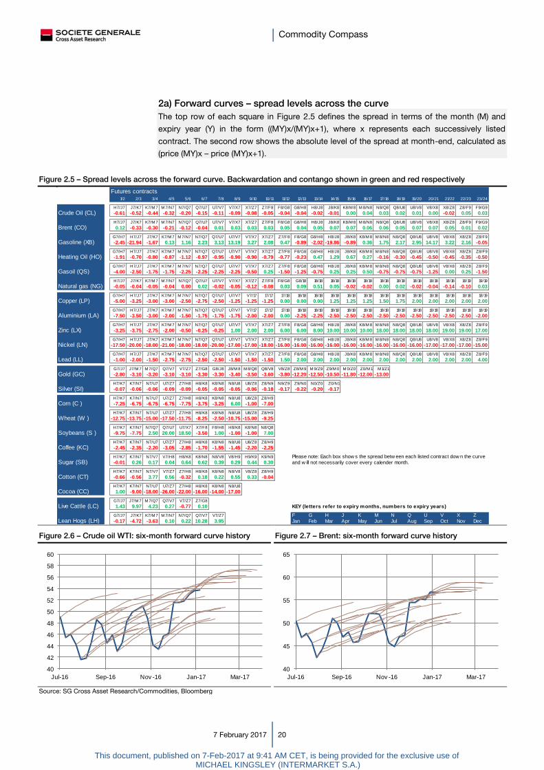
2a) Forward curves – spread levels across the curve

The top row of each square in Figure 2.5 defines the spread in terms of the month (M) and

expiry year (Y) in the form ((MY)x/(MY)x+1), where x represents each successively listed

contract. The second row shows the absolute level of the spread at month-end, calculated as

(price (MY)x – price (MY)x+1).

Figure 2.5 – Spread levels across the forward curve. Backwardation and contango shown in green and red respectively

Figure 2.6 – Crude oil WTI: six-month forward curve history Figure 2.7 – Brent: six-month forward curve history


Futures contracts1/2 2/3 3/4 4/5 5/6 6/7 7/8 8/9 9/10 10/11 11/12 12/13 13/14 14/15 15/16 16/17 17/18 18/19 19/20 20/21 21/22 22/23 23/24

H7/J7 J7/K7 K7/M 7 M 7/N7 N7/Q7 Q7/U7 U7/V7 V7/X7 X7/Z7 Z7/F8 F8/G8 G8/H8 H8/J8 J8/K8 K8/M 8 M 8/N8 N8/Q8 Q8/U8 U8/V8 V8/X8 X8/Z8 Z8/F9 F9/G9

-0.61 -0.52 -0.44 -0.32 -0.20 -0.15 -0.11 -0.09 -0.08 -0.05 -0.04 -0.04 -0.02 -0.01 0.00 0.04 0.03 0.02 0.01 0.00 -0.02 0.05 0.03

H7/J7 J7/K7 K7/M 7 M 7/N7 N7/Q7 Q7/U7 U7/V7 V7/X7 X7/Z7 Z7/F8 F8/G8 G8/H8 H8/J8 J8/K8 K8/M 8 M 8/N8 N8/Q8 Q8/U8 U8/V8 V8/X8 X8/Z8 Z8/F9 F9/G9

0.12 -0.33 -0.30 -0.21 -0.12 -0.04 0.01 0.03 0.03 0.03 0.05 0.04 0.05 0.07 0.07 0.06 0.06 0.05 0.07 0.07 0.05 0.01 0.02

G7/H7 H7/J7 J7/K7 K7/M 7 M 7/N7 N7/Q7 Q7/U7 U7/V7 V7/X7 X7/Z7 Z7/F8 F8/G8 G8/H8 H8/J8 J8/K8 K8/M 8 M 8/N8 N8/Q8 Q8/U8 U8/V8 V8/X8 X8/Z8 Z8/F9

-2.45 -21.94 -1.67 0.13 1.16 2.23 3.13 13.19 3.27 2.08 0.47 -0.89 -2.02 -19.86 -0.89 0.36 1.75 2.17 2.95 14.17 3.22 2.16 -0.05


-1.91 -0.70 -0.80 -0.87 -1.12 -0.97 -0.95 -0.90 -0.90 -0.79 -0.77 -0.23 0.47 1.29 0.67 0.27 -0.16 -0.30 -0.45 -0.50 -0.45 -0.35 -0.50


-4.00 -2.50 -1.75 -1.75 -2.25 -2.25 -2.25 -2.25 -0.50 0.25 -1.50 -1.25 -0.75 0.25 0.25 0.50 -0.75 -0.75 -0.75 -1.25 0.00 0.25 -1.50

H7/J7 J7/K7 K7/M 7 M 7/N7 N7/Q7 Q7/U7 U7/V7 V7/X7 X7/Z7 Z7/F8 F8/G8 G8/18 18/18 18/18 18/18 18/18 18/18 18/18 18/18 18/18 18/18 18/19 19/19

-0.05 -0.04 -0.05 -0.04 0.00 0.02 -0.02 -0.05 -0.12 -0.08 0.03 0.09 0.51 0.05 -0.02 -0.02 0.00 0.02 -0.02 -0.04 -0.14 -0.10 0.03

G7/H7 H7/J7 J7/K7 K7/M 7 M 7/N7 N7/Q7 Q7/U7 U7/V7 V7/17 17/17 17/18 18/18 18/18 18/18 18/18 18/18 18/18 18/18 18/18 18/18 18/18 18/18 18/19

-5.00 -3.25 -3.00 -3.00 -2.50 -2.75 -2.50 -1.25 -1.25 -1.25 0.00 0.00 0.00 1.25 1.25 1.25 1.50 1.75 2.00 2.00 2.00 2.00 2.00

G7/H7 H7/J7 J7/K7 K7/M 7 M 7/N7 N7/Q7 Q7/U7 U7/V7 V7/17 17/17 17/18 18/18 18/18 18/18 18/18 18/18 18/18 18/18 18/18 18/18 18/18 18/18 18/19

-7.50 -3.50 -3.00 -2.00 -1.50 -1.75 -1.75 -1.75 -2.00 -2.00 0.00 -2.25 -2.25 -2.50 -2.50 -2.50 -2.50 -2.50 -2.50 -2.50 -2.50 -2.50 -2.00


-3.25 -3.75 -2.75 -2.00 -0.50 -0.25 -0.25 1.00 2.00 2.00 6.00 6.00 8.00 10.00 10.00 10.00 18.00 18.00 18.00 18.00 19.00 19.00 17.00


-17.50 -20.00 -18.00 -21.00 -18.00 -18.00 -20.00 -17.00 -17.00 -18.00 -16.00 -16.00 -16.00 -16.00 -16.00 -16.00 -16.00 -16.00 -16.00 -17.00 -17.00 -17.00 -15.00


-1.00 -2.00 -1.50 -2.75 -2.75 -2.50 -2.50 -1.50 -1.50 -1.50 1.50 2.00 2.00 2.00 2.00 2.00 2.00 2.00 2.00 2.00 2.00 2.00 4.00

G7/J7 J7/M 7 M 7/Q7 Q7/V7 V7/Z7 Z7/G8 G8/J8 J8/M 8 M 8/Q8 Q8/V8 V8/Z8 Z8/M 9 M 9/Z9 Z9/M 0 M 0/Z0 Z0/M 1 M 1/Z1

-2.80 -3.10 -3.20 -3.10 -3.10 -3.30 -3.30 -3.40 -3.50 -3.60 -3.80 -12.20 -12.50 -10.50 -11.80 -12.00 -13.00

H7/K7 K7/N7 N7/U7 U7/Z7 Z7/H8 H8/K8 K8/N8 N8/U8 U8/Z8 Z8/N9 N9/Z9 Z9/N0 N0/Z0 Z0/N1

-0.07 -0.06 -0.06 -0.09 -0.09 -0.05 -0.05 -0.05 -0.06 -0.18 -0.17 -0.22 -0.20 -0.17

H7/K7 K7/N7 N7/U7 U7/Z7 Z7/H8 H8/K8 K8/N8 N8/U8 U8/Z8 Z8/H9

-7.25 -6.75 -6.75 -6.75 -7.75 -3.75 -3.25 6.00 -1.00 -7.00


-12.75 -13.75 -15.00 -17.50 -11.75 -8.25 -2.50 -10.75 -15.00 -9.25

H7/K7 K7/N7 N7/Q7 Q7/U7 U7/X7 X7/F8 F8/H8 H8/K8 K8/N8 N8/Q8

-9.75 -7.75 2.50 20.00 18.50 -3.50 1.00 -1.00 -1.00 7.00


-2.45 -2.35 -2.20 -3.05 -2.85 -1.70 -1.55 -1.45 -2.20 -2.25

H7/K7 K7/N7 N7/V7 V7/H8 H8/K8 K8/N8 N8/V8 V8/H9 H9/K9 K9/N9 Please note: Each box show s the spread betw een each listed contract dow n the curve

-0.01 0.26 0.17 0.04 0.64 0.62 0.39 0.29 0.44 0.30 and w ill not necessarily cover every calender month.

H7/K7 K7/N7 N7/V7 V7/Z7 Z7/H8 H8/K8 K8/N8 N8/V8 V8/Z8 Z8/H9

-0.66 -0.56 3.77 0.56 -0.32 0.18 0.22 0.55 0.33 -0.04

H7/K7 K7/N7 N7/U7 U7/Z7 Z7/H8 H8/K8 K8/N8 N8/U8

1.00 -9.00 -18.00 -26.00 -22.00 -16.00 -14.00 -17.00

G7/J7 J7/M 7 M 7/Q7 Q7/V7 V7/Z7 Z7/G8

1.43 9.97 4.23 0.27 -0.77 0.10 KEY (letters refer to expiry months, numbers to expiry years)

G7/J7 J7/K7 K7/M 7 M 7/N7 N7/Q7 Q7/V7 V7/Z7 F G H J K M N Q U V X Z

-0.17 -4.72 -3.63 0.10 0.22 10.28 3.95 Jan Feb Mar Apr May Jun Jul Aug Sep Oct Nov Dec

Cotton (CT)

Cocoa (CC)

Live Cattle (LC)

Lean Hogs (LH)

Silver (SI)

Corn (C )

Wheat (W )

Soybeans (S )

Coffee (KC)

Sugar (SB)

Gold (GC)

Crude Oil (CL)

Brent (CO)

Gasoline (XB)

Heating Oil (HO)

Gasoil (QS)

Natural gas (NG)

Copper (LP)

Aluminium (LA)

Zinc (LX)

Nickel (LN)

Lead (LL)

40

42

44

46

48

50

52

54

56

58

60

Jul-16 Sep-16 Nov -16 Jan-17 Mar-17

40

45

50

55

60

65

Jul-16 Sep-16 Nov -16 Jan-17 Mar-17


Commodity Compass

7 February 2017 21

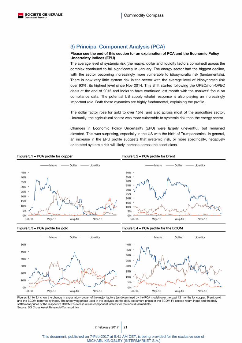
3) Principal Component Analysis (PCA)

Please see the end of this section for an explanation of PCA and the Economic Policy

Uncertainty Indices (EPU)

The average level of systemic risk (the macro, dollar and liquidity factors combined) across the

complex continued to fall significantly in January. The energy sector had the biggest decline,

with the sector becoming increasingly more vulnerable to idiosyncratic risk (fundamentals).

There is now very little system risk in the sector with the average level of idiosyncratic risk

over 93%, its highest level since Nov 2014. This shift started following the OPEC/non-OPEC

deals at the end of 2016 and looks to have continued last month with the markets’ focus on

compliance data. The potential US supply (shale) response is also playing an increasingly

important role. Both these dynamics are highly fundamental, explaining the profile.

The dollar factor rose for gold to over 15%, and also across most of the agriculture sector.

Unusually, the agricultural sector was more vulnerable to systemic risk than the energy sector.

Changes in Economic Policy Uncertainty (EPU) were largely uneventful, but remained

elevated. This was surprising, especially in the US with the birth of Trumponomics. In general,

an increase in the EPU profile suggests that systemic risk, or more specifically, negatively

orientated systemic risk will likely increase across the asset class.

Figure 3.1 – PCA profile for copper Figure 3.2 – PCA profile for Brent

Figure 3.3 – PCA profile for gold Figure 3.4 – PCA profile for the BCOM

Figures 3.1 to 3.4 show the change in explanatory power of the major factors (as determined by the PCA model) over the past 12 months for copper, Brent, gold

and the BCOM commodity index. The underlying prices used in the analysis are the daily settlement prices of the BCOM F3 excess return index and the daily

settlement prices of the respective BCOM F3 excess return component indices for the individual markets.


0%

5%

10%

15%

20%

25%

30%

35%

40%

45%

Feb-16 May -16 Aug-16 Nov -16

Macro Dollar Liquidity

0%

5%

10%

15%

20%

25%

30%

35%

40%

45%

50%



0%

10%

20%

30%

40%

50%

60%



0%

5%

10%

15%

20%

25%

30%

35%

40%




Commodity Compass

7 February 2017 22

Figure 3.5 – PCA analysis: change in profile over the month

Figure 3.5 shows the change in explanatory power for each of the major factors across 22 major commodity markets and the BCOM commodity index over the

month. The underlying prices used in the analysis are the daily settlement prices of the BCOM F3 excess return index and the daily settlement prices of the

respective BCOM F3 excess return component indices for the individual markets. The average shown at the bottom of the table is the equally-weighted arithmetic

mean of the 22 markets. The average value will differ from the BCOM value due to weighting and correlation effects.


Figure 3.6 – Historical PCA profile of the BCOM commodity index since 2008


PCA explained:

Principal Component Analysis (PCA) is a statistical tool that allows us to break down commodity price returns and isolate the major explanatory variables. SG has

developed a PCA model, specifically for commodity markets, that uses 23 different non-fundamental variables. These include measures of inflation, currency

changes, credit spreads, implied volatility, equity and changes in equity indices. These variables are simplified into three principal components through the PCA

process. Each component is a linear combination of the original 23 variables that can be mapped to a “real world” factor by examining and interpreting the

underlying weightings of these variables. The first factor is defined as a macro-related factor, the second a currency factor, and the third an interest rate or liquidity

factor. Each of the three factors is linearly regressed against each commodity to determine the explanatory power each factor has on the variance of that

commodity. The residual, or that which is not explained by the regression process, is attributed to fundamentals (specific commodity supply & demand dynamics).

Macro Dollar Liquidity Fundamental Macro Dollar Liquidity Fundamental

Aluminium 4.07% 0.00% 0.83% 95.09% 2.99% 1.77% 4.47% 90.76%

Copper 15.64% 1.27% 9.47% 73.58% 9.43% 3.08% 15.54% 71.94%

Lead 1.69% 0.96% 4.09% 93.24% 2.86% 4.03% 5.86% 87.25%

Nickel 10.96% 4.66% 1.65% 82.76% 16.28% 6.50% 6.09% 71.14%

Zinc 2.44% 0.25% 12.09% 85.22% 4.77% 3.37% 10.86% 81.00%

Gold 18.33% 15.08% 1.80% 64.79% 19.32% 5.13% 5.69% 69.85%

Silver 3.32% 11.46% 1.93% 83.29% 4.20% 14.51% 0.52% 80.78%

Crude Oil (WTI) 2.25% 7.32% 0.30% 90.12% 11.88% 9.07% 0.15% 78.90%

Brent 1.85% 7.20% 0.41% 90.53% 10.94% 9.41% 0.24% 79.41%

Heating Oil 0.31% 4.75% 0.51% 94.42% 6.60% 12.16% 0.02% 81.23%

Gasoline 0.04% 4.90% 0.41% 94.64% 3.07% 8.73% 0.11% 88.08%

Gasoil 0.08% 6.27% 0.39% 93.25% 3.58% 15.99% 0.42% 80.00%

Natural Gas 1.18% 0.69% 1.67% 96.47% 0.37% 0.00% 0.02% 99.61%

Corn 1.48% 14.27% 0.04% 84.22% 0.60% 6.07% 0.01% 93.32%

Wheat 3.17% 9.70% 0.05% 87.08% 2.19% 0.59% 2.69% 94.54%

Soybeans 0.29% 9.53% 0.19% 89.98% 0.39% 4.93% 0.02% 94.66%

Cotton 0.22% 2.78% 1.14% 95.86% 0.01% 0.88% 0.00% 99.10%

Sugar 3.04% 4.68% 3.89% 88.40% 1.99% 0.04% 2.84% 95.13%

Coffee 0.54% 7.87% 0.16% 91.44% 0.18% 0.22% 3.66% 95.94%

Cocoa 5.38% 2.82% 0.83% 90.96% 11.25% 0.42% 0.19% 88.15%

Live Cattle 0.20% 0.35% 0.01% 99.45% 0.35% 0.13% 0.10% 99.42%

Lean Hogs 3.68% 6.32% 0.81% 89.16% 1.85% 1.38% 0.00% 96.77%

BCOM 0.42% 15.53% 0.13% 83.89% 6.75% 15.98% 0.06% 77.20%

AVERAGE 3.64% 5.60% 1.94% 88.82% 5.23% 4.93% 2.70% 87.13%

January-2017 December-2016

0%

10%

20%

30%

40%

50%

60%

70%

80%

90%

100%

2008 2009 2010 2011 2012 2013 2014 2015 2016

Macro Dollar Liquidity Fundamentals


Commodity Compass

7 February 2017 23

3a) Economic Policy Uncertainty (EPU) Indices

Economic Policy Uncertainty (EPU) is a class of economic risk where the future path of

government policy is uncertain. Policy uncertainty may refer to uncertainty about monetary or

fiscal policy, the tax or regulatory regime, or uncertainty over electoral outcomes that will

influence political leadership.

In the context of our PCA analysis (Section 3), changes in EPU can lead to changes in

systemic risk. Specifically, increases in EPU are associated with negatively orientated

systemic risk. In order to track these changes, we use the EPU indices, developed by

Economic Policy Uncertainty4

Figure 3.7 – Monthly EPU indices for the US, EU and China. Increases (decreases) in the indices

show rising (declining) EPU


Figure 3.8 – Monthly changes in the US, EU and China EPU Index. Black line illustrates standard deviation (12m rolling) threshold.

Changes in EPU in excess of this threshold are significant (red bars) and are associated with commodity price weakness


Economic Policy Indices:

The Baker, Bloom and Davis news-based index of economic policy uncertainty for the US is based on the frequency of newspaper references to policy uncertainty.

10 large newspapers are used.

The European Policy Index is constructed based on newspaper articles regarding policy uncertainty.

The China Index is constructed using a scaled frequency count of articles about policy-related economic uncertainty in the South China Morning Post (SCMP),

Hong Kong's leading English-language newspaper. The method follows our news-based indices of economic policy uncertainty for the US and other countries.

We only consider the news-flow EPU Indices.

Source: www.policyuncertainty.com.

4 Baker, Scott; Bloom, Nick; Davis, Steven (2011). "Measuring Policy Uncertainty?" (PDF). Stanford Mimeo.

0

100

200

300

400

500

600

700

800

Jan-07 Jan-09 Jan-11 Jan-13 Jan-15 Jan-17

US Europe China

-100%

-50%

0%

50%

100%

150%

200%

Feb-12 Feb-13 Feb-14 Feb-15 Feb-16

US

-100%

-50%

0%

50%

100%

150%


Europe

-100%

-50%

0%

50%

100%

150%

200%


China


http://www.policyuncertainty.com/

http://www.policyuncertainty.com/

http://www.policyuncertainty.com/media/BakerBloomDavis.pdf

Commodity Compass

7 February 2017 24

4) Cost curve dynamics - the SG Production Cost Model

Changes in currencies, inflation, energy costs and metal prices can have a profound impact

on mining costs. Understanding the impact of these changes is critical in assessing how

individual mining costs and, by extension, broader industry cost curves are evolving. The

model provides a more accurate and timely assessment of the cost curve, allowing the current

level of price support and the likelihood of cuts in mine supply to be more accurately

addressed. The model is described in the SG Production Cost Model (SG PCM) publication.

Figure 4.1 – Changes in the Cost Floor (90th Percentile) – Using the Spot Price (SPM) Methodology. The implied cost floor is

shown in blue, the published cost floor in brown

Source: SG Cross Asset Research/Commodities, SNL Metals & Mining , Bloomberg

Figure 4.2 – Copper – Industry costs vs SG PCM implied costs.

Implied costs derived from 199 mines (SPM)

Figure 4.3 – Zinc – Industry costs vs SG PCM implied costs.


Figure 4.4 – Lead – Industry costs vs SG PCM implied costs.


Figure 4.5 – Nickel – Industry costs vs SG PCM implied costs.


SPM = Spot Price Methodology, “Industry” refers to the 90th percentile total cash costs (SNL Metals & Mining)

Source: SG Cross Asset Research/Commodities, SNL Metals & Mining, Bloomberg

Metal Price

90th

Percentile

Implied Cost

(PCM)

Change in

Cost Floor ($)

Change in

Cost Floor (%)

Price - Cost

Floor ($)

Price - Cost

Floor (%)

Copper $5,536 $3,929 $4,057 $127 3.24% $1,479 36.45%

Zinc $2,576 $1,548 $1,481 -$67 -4.34% $1,095 73.98%

Lead $2,017 $1,390 $1,427 $37 2.63% $590 41.33%

Nickel $10,020 $11,478 $10,698 -$780 -6.80% -$678 -6.33%

* Total Cash Costs (SNL M etals & M ining)

SPOT PRICE METHODOLOGY

3500

4000

4500

5000

5500

6000

6500

Jan-16 Apr-16 Jul-16 Oct-16 Jan-17

Price Industry Implied (SPM)

1200

1400

1600

1800

2000

2200

2400

2600

2800

3000



1200

1400

1600

1800

2000

2200

2400

2600



7000

7500

8000

8500

9000

9500

10000

10500

11000

11500

12000





Commodity Compass

7 February 2017 25

4a) Individual mine analysis

The following charts illustrate how the most recently reported total cash costs - defined as the

sum of all minesite costs (mining + milling), transport and offsite costs, smelting and refining

costs and royalties - have been impacted by changes in the underlying cost drivers (currency

movements, inflation, oil (fuel) prices, treatment and refining charges and the metal prices

themselves).

Each bubble represents a mine – the area of the bubble is a function of its most recently

reported total annual production (scaled across all metals). The position on the x-axis is driven

by the most recently reported total cash cost (sourced from SNL, Metals & Mining5) and the

position on the y-axis is the extent by which the total cash cost has been shifted by recent

changes in the Cost Drivers using our Spot Price Methodology.

Please refer to the SG Production Cost Model (SG PCM) publication for full details.

Figure 4.6 – Copper – Change in total cash costs for all mines in

the top ten largest producing countries

Figure 4.7 – Zinc – Change in total cash costs for all mines in the

top ten largest producing countries

Figure 4.8 – Lead – Change in total cash costs for all mines in


Figure 4.9 – Nickel – Change in total cash costs for all mines in



Country labels at the bottom of each chart run from the smallest producer (top left) to the largest producer (bottom right)

5 The following document produced by SNL Metals & Mining methodology and definitions provides a detailed overview

of SNL’s principals and methodologies.

-20%

-15%

-10%

-5%

0%

5%

10%

15%

500 1500 2500 3500 4500 5500 6500

Russia Poland Mexico Indonesia Canada

Zambia Australia Peru USA Chile

-20%

-15%

-10%

-5%

0%

5%

700 900 1100 1300 1500 1700 1900 2100

Namibia Boliv ia Ireland Sweden Canada

Mexico India USA Peru Australia

-20%

-15%

-10%

-5%

0%

5%

10%

400 900 1400 1900

Morocco Ireland South Af rica Boliv ia Sweden

India Peru Mexico USA Australia

-20%

-15%

-10%

-5%

0%

5%

10%

15%

-5000 0 5000 10000 15000 20000 25000

Philippines South Af rica Cuba Japan

New Caledonia Brazil Indonesia Canada

Australia Russia



https://www.snl.com/help/Mine_Economics_Methodology.htm

Commodity Compass

7 February 2017 26

5) CFTC Commitment of Trader (COT) analysis

The following charts show the trends and extremes in the Money Manager (MM) and

producer/merchant/processor/user (PMPU) sub-categories of the COT report for the major

commodity markets. In Section 5a, we show the new (since 2014) LME COT data for copper,

aluminium, zinc, lead and nickel. Large MM long and short positions indicate that speculative

can be vulnerable to sudden price reversals if positions unwind quickly. Trends in the PMPU

positioning are often indicative of future price dynamics, as it is widely accepted that the

PMPU category possesses an informational edge. By plotting changes in the long and short

positions independently, the drivers of net positioning become clearer.

Below are a few key highlights and observations from the charts below:

Both long PMPU (consumer) and short PMPU (producer) hedging in WTI continued to

increase. Producers, as a % of OI, are currently the most hedged they have been since mid

2007. Short PMPU (producer) hedging in Natural gas dramatically increased, with the market

currently as a % of OI, the most hedged it has even been. Long MM liquidation in gold

continued, but the short selling ceased. The long MM position in copper and aluminium

remained near record highs with the short positions remaining small and unchanged.

Figure 5.1 – Crude oil MM positions - % of total open interest Figure 5.2 – Crude oil PMPU positions - % of total open interest

Figure 5.3 – Natural gas MM positions - % of total open interest Figure 5.4 – Nat. gas PMPU positions - % of total open interest

Data is as of the most recent COT report with graphs extending back to the inception of the disaggregated data (June 2006). The shaded regions in each chart

show the historical range of the individual long (light blue) and short (light grey) positions. The lines on each chart show the actual historical long (dark blue) and

short (dark grey) positions, with the net position shown in orange. All positions are expressed as a percentage of open interest. Data includes only futures.

Producer/merchant/processor/user is an entity that predominantly engages in the production, processing, packing or handling of a physical commodity and

uses the futures markets to manage or hedge risks associated with those activities. Money manager for the purpose of this report is a registered commodity

trading advisor (CTA); a registered commodity pool operator (CPO); or an unregistered fund identified by CFTC. These traders are engaged in managing and

conducting organised futures trading on behalf of clients.

Source: SG Cross Asset Research/Commodities, Bloomberg, www.cftc.gov

-15%

-10%

-5%

0%

5%

10%

15%

20%

25%

2006 2007 2008 2009 2010 2011 2012 2013 2014 2015 2016

Long Range Short Range Long Position

Short Position Net Position

-50%

-40%

-30%

-20%

-10%

0%

10%

20%

30%

40%

2006 2007 2008 2009 2010 2011 2012 2013 2014 2015 2016



-50%

-40%

-30%

-20%

-10%

0%

10%

20%

30%

40%

2006 2007 2008 2009 2010 2011 2012 2013 2014 2015 2016



-30%

-25%

-20%

-15%

-10%

-5%

0%

5%

10%

15%

20%

25%

2006 2007 2008 2009 2010 2011 2012 2013 2014 2015 2016




http://www.cftc.gov/

Commodity Compass

7 February 2017 27

Figure 5.5 – Gold MM positions- % of total open interest Figure 5.6 – Gold PMPU positions- % of total open interest

Figure 5.7 – Corn MM positions- % of total open interest Figure 5.8 – Wheat MM positions- % of total open interest

Figure 5.9 – Soybean MM positions- % of total open interest Figure 5.10 – Cotton MM positions- % of total open interest

Data is as of the most recent COT report with graphs extending back to the inception of the disaggregated data (June 2006). The shaded regions in each chart

show the historical range of the individual long (light blue) and short (light grey) positions. The lines on each chart show the actual historical long (dark blue) and

short (dark grey) positions, with the net position shown in orange. All positions are expressed as a percentage of open interest. Data includes only futures.

Producer/merchant/processor/user is an entity that predominantly engages in the production, processing, packing or handling of a physical commodity and

uses the futures markets to manage or hedge risks associated with those activities. Money manager for the purpose of this report is a registered commodity

trading advisor (CTA); a registered commodity pool operator (CPO); or an unregistered fund identified by CFTC. These traders are engaged in managing and

conducting organised futures trading on behalf of clients.


-40%

-30%

-20%

-10%

0%

10%

20%

30%

40%

50%

60%

2006 2007 2008 2009 2010 2011 2012 2013 2014 2015 2016



-70%

-60%

-50%

-40%

-30%

-20%

-10%

0%

10%

20%

30%

40%

2006 2007 2008 2009 2010 2011 2012 2013 2014 2015 2016



-40%

-30%

-20%

-10%

0%

10%

20%

30%

40%

2006 2007 2008 2009 2010 2011 2012 2013 2014 2015 2016



-60%

-50%

-40%

-30%

-20%

-10%

0%

10%

20%

30%

40%

2006 2007 2008 2009 2010 2011 2012 2013 2014 2015 2016



-30%

-20%

-10%

0%

10%

20%

30%

40%

2006 2007 2008 2009 2010 2011 2012 2013 2014 2015 2016



-40%

-30%

-20%

-10%

0%

10%

20%

30%

40%

50%

2006 2007 2008 2009 2010 2011 2012 2013 2014 2015 2016





Commodity Compass

7 February 2017 28

5a) London Metal Exchange (LME) COT Analysis

The following LME COT data is available since July 2014.

Figure 5.11 – Copper MM positions- % of total open interest Figure 5.12 – Copper PMPU positions- % of total open interest

Figure 5.13 – Aluminium MM positions- % of total open interest Figure 5.14 – Zinc MM positions- % of total open interest

Figure 5.15 – Lead MM positions- % of total open interest Figure 5.16 – Nickel MM positions- % of total open interest

Data is as of the most recent COT report with graphs extending back to the inception of the data (July 2014). The shaded regions in each chart show the historical

range of the individual long (light red) and short (light brown) positions. The lines on each chart show the actual historical long (dark red) and short (dark brown)

positions, with the net position shown in blue. All positions are expressed as a percentage of open interest. Data includes only futures.

Producer/merchant/processor/user Entities that are predominantly engaged in production, processing, packaging or handling of metal and that use the LME to

manage or hedge risks associated with those activities. Money manager Entities that are engaged in managing and conducting LME contracts on behalf of

underlying Clients such as investment fund firms.

Source: SG Cross Asset Research/Commodities, Bloomberg, www.lme.com

-30%

-20%

-10%

0%

10%

20%

30%

40%

Jul-14 Jan-15 Jul-15 Jan-16 Jul-16



-50%

-40%

-30%

-20%

-10%

0%

10%

20%

30%

40%




-40%

-30%

-20%

-10%

0%

10%

20%

30%

40%




-30%

-20%

-10%

0%

10%

20%

30%

40%

50%




-50%

-40%

-30%

-20%

-10%

0%

10%

20%

30%

40%




-40%

-30%

-20%

-10%

0%

10%

20%

30%

40%





http://www.lme.com/

Commodity Compass

7 February 2017 29

6) Dry Powder analysis – insights into positioning

In the October 2016 Commodities Compass - Measuring “dry powder” in commodities –

some alternative insights into positioning, we looked at alternative ways of analysing

commodity COT Money Manager (MM) positioning data. We provided additional insights into

gauging the likelihood of further investment flows based on historical allocation patterns, the

number of entities currently in the market, the current position limits and of course current

prices.

This approach essentially allows us to determine the amount of “dry powder” there is in each

commodity to support a potential move. The approach also provides additional insight into

market positioning and significant value in assessing trade conviction and identifying new

trading opportunities.

A key benefit of this approach is that it helps us answer some of the following types of

questions: Are there many entities left to buy/sell the market? How much capital could be

potentially allocated to a position at current prices? How close are the current positions to

position limits? How vulnerable are current positions to profit-taking (long liquidation or short

covering)? How strong could the potential price retracements and rallies be? Here we provide

updates of charts for some of the key commodities.

Below we highlight a few interesting observations from the charts below:

WTI

As described in our previous Compass, the likelihood of the long futures position in WTI

(Figure 6.1) Managers (MMs) increasing was discussed. With the futures position near record

highs, but the number of long traders still relatively low, the most obvious way for this to

happen would be for new long traders to enter the market. Interestingly however, the current

mismatch between the size of the futures position and the dollar position (due to low oil

prices) provided an alternative way. Due to the low dollar exposure, the existing long position,

which even though is near record size in terms of OI, could easily be increased without

necessarily breeching any exposure limits. Both these scenarios were discussed.

Last month the long position rose to record high, as the dollar exposure on the existing

position was in fact increased. This is now at normal levels (on the trend line) given the

number of long traders, which suggests that going forward, for the position to expand further,

new traders will likely need to enter the market.

In terms of the stability of the current position, the size (in lots) of both the long and short

positions suggests the market is vulnerable to significant long liquidation/ short covering.

Cotton

The long and short futures and dollar positions (Figures 6.9 & 6.10) continue to be at opposite

extremes, with the longs at historical maxima (and having expanded slightly last month) and

the shorts near historical minima. This suggests that MM driven upside is largely limited (due

to simple absence of any dry powder), whereas the downside risk via long liquidation and

fresh shorts could be considerable.

Natural gas

As discussed in our previous Compass, the downside risk via long liquidation and fresh shorts

was considerable; this has now reduced after the 16% fall in price last month.






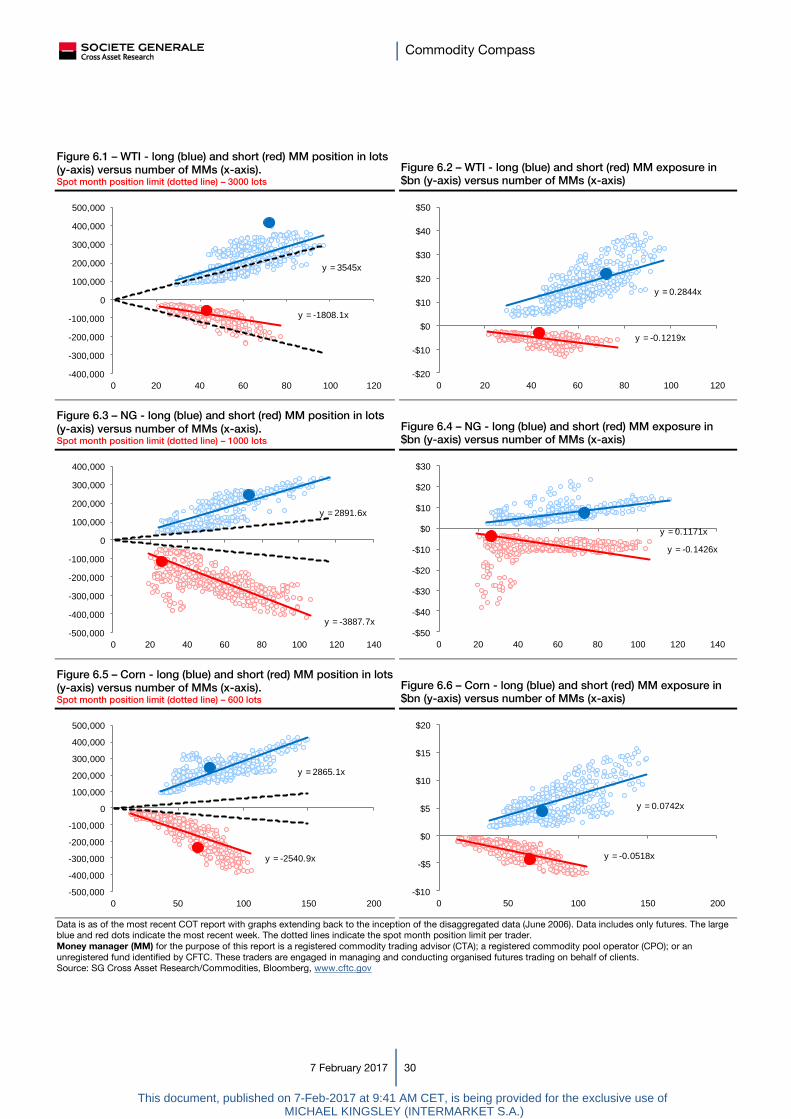
Commodity Compass

7 February 2017 30

Figure 6.1 – WTI - long (blue) and short (red) MM position in lots

(y-axis) versus number of MMs (x-axis). Spot month position limit (dotted line) – 3000 lots

Figure 6.2 – WTI - long (blue) and short (red) MM exposure in

$bn (y-axis) versus number of MMs (x-axis)

Figure 6.3 – NG - long (blue) and short (red) MM position in lots


Figure 6.4 – NG - long (blue) and short (red) MM exposure in


Figure 6.5 – Corn - long (blue) and short (red) MM position in lots


Figure 6.6 – Corn - long (blue) and short (red) MM exposure in


Data is as of the most recent COT report with graphs extending back to the inception of the disaggregated data (June 2006). Data includes only futures. The large

blue and red dots indicate the most recent week. The dotted lines indicate the spot month position limit per trader.

Money manager (MM) for the purpose of this report is a registered commodity trading advisor (CTA); a registered commodity pool operator (CPO); or an

unregistered fund identified by CFTC. These traders are engaged in managing and conducting organised futures trading on behalf of clients.


y = 3545x

y = -1808.1x

-400,000

-300,000

-200,000

-100,000

0

100,000

200,000

300,000

400,000

500,000

0 20 40 60 80 100 120

y = 0.2844x

y = -0.1219x

-$20

-$10

$0

$10

$20

$30

$40

$50

0 20 40 60 80 100 120

y = 2891.6x

y = -3887.7x

-500,000

-400,000

-300,000

-200,000

-100,000

0

100,000

200,000

300,000

400,000

0 20 40 60 80 100 120 140

y = 0.1171x

y = -0.1426x

-$50

-$40

-$30

-$20

-$10

$0

$10

$20

$30

0 20 40 60 80 100 120 140

y = 2865.1x

y = -2540.9x

-500,000

-400,000

-300,000

-200,000

-100,000

0

100,000

200,000

300,000

400,000

500,000

0 50 100 150 200

y = 0.0742x

y = -0.0518x

-$10

-$5

$0

$5

$10

$15

$20

0 50 100 150 200



Commodity Compass

7 February 2017 31

Figure 6.7 – Soybeans - long (blue) and short (red) MM position

in lots (y-axis) versus number of MMs (x-axis). Spot month position limit (dotted line) – 600 lots

Figure 6.8 – Soybeans - long (blue) and short (red) MM

exposure in $bn (y-axis) versus number of MMs (x-axis)

Figure 6.9 – Cotton - long (blue) and short (red) MM position in

lots (y-axis) versus number of MMs (x-axis). Spot month position limit (dotted line) – 300 lots

Figure 6.10 – Cotton - long (blue) and short (red) MM exposure

in $bn (y-axis) versus number of MMs (x-axis)

Figure 6.11 – Sugar - long (blue) and short (red) MM position in


Figure 6.12 – Sugar - long (blue) and short (red) MM exposure in




Money manager for the purpose of this report is a registered commodity trading advisor (CTA); a registered commodity pool operator (CPO); or an unregistered

fund identified by CFTC. These traders are engaged in managing and conducting organised futures trading on behalf of clients.


y = 1477x

y = -1115.6x

-200,000

-150,000

-100,000

-50,000

0

50,000

100,000

150,000

200,000

250,000

300,000

0 50 100 150 200

y = 0.0912x

y = -0.0556x

-$10

-$5

$0

$5

$10

$15

$20

$25

0 50 100 150 200

y = 724.21x

y = -638.45x

-80,000

-60,000

-40,000

-20,000

0

20,000

40,000

60,000

80,000

100,000

120,000

0 20 40 60 80 100 120

y = 0.0284x

y = -0.0205x

-$3

-$2

-$1

$0

$1

$2

$3

$4

$5

0 20 40 60 80 100 120

y = 3416.8x

y = -3212.6x

-500,000

-400,000

-300,000

-200,000

-100,000

0

100,000

200,000

300,000

400,000

500,000

0 20 40 60 80 100

y = 0.0704x

y = -0.0535x

-$6

-$4

-$2

$0

$2

$4

$6

$8

0 20 40 60 80 100



Commodity Compass

7 February 2017 32

Figure 6.13 – Gold - long (blue) and short (red) MM position in


Figure 6.14 – Gold - long (blue) and short (red) MM exposure in


Figure 6.15 – Silver - long (blue) and short (red) MM position in


Figure 6.16 – Silver - long (blue) and short (red) MM exposure in


Figure 6.17 – Live cattle - long (blue) and short (red) MM position

in lots (y-axis) versus number of MMs (x-axis). Spot month position limit (dotted line) – 450 lots

Figure 6.18 – Live cattle - long (blue) and short (red) MM

exposure in $bn (y-axis) versus number of MMs (x-axis)



Money manager for the purpose of this report is a registered commodity trading advisor (CTA); a registered commodity pool operator (CPO); or an unregistered

fund identified by CFTC. These traders are engaged in managing and conducting organised futures trading on behalf of clients.


y = 1902.7x

y = -1271.9x

-500,000

-400,000

-300,000

-200,000

-100,000

0

100,000

200,000

300,000

400,000

500,000

0 20 40 60 80 100 120 140

y = 0.2354x

y = -0.153x

-$20

-$10

$0

$10

$20

$30

$40

$50

0 20 40 60 80 100 120 140

y = 964.01x

y = -809.03x

-150,000

-100,000

-50,000

0

50,000

100,000

150,000

0 20 40 60 80

y = 0.0942x

y = -0.0734x

-$6

-$4

-$2

$0

$2

$4

$6

$8

$10

$12

0 20 40 60 80

y = 1144.6x

y = -727.5x

-100,000

-50,000

0

50,000

100,000

150,000

200,000

0 20 40 60 80 100 120 140

y = 0.0543x

y = -0.0324x

-$6

-$4

-$2

$0

$2

$4

$6

$8

$10

0 20 40 60 80 100 120 140



Commodity Compass

7 February 2017 33

7) SG price forecasts

The following charts show the average annual SG price forecasts over the next three years.

The current year is based on the average of the forthcoming quarterly forecasts. For

detailed forecasts, please refer to our quarterly Commodities Review publications.

Forecast years are indicated by the following colours:

Figure 7.1 – Crude oil (WTI) Figure 7.2 – Brent

Figure 7.3 – Natural gas (NYMEX) Figure 7.4 – Copper (LME)

Figure 7.5 – Aluminium Figure 7.6 – Zinc

Price history (grey line) is based on the front month futures contract (unadjusted).


2017 2018 2019

20

30

40

50

60

70

80

90

100

110

120

2014 2015 2016 2017 2018 2019

Forward Curv e 54.75 62.50 67.00

20

30

40

50

60

70

80

90

100

110

120

2014 2015 2016 2017 2018 2019

Forward Curv e 56.25 65.00 70.00

1.00

2.00

3.00

4.00

5.00

6.00

7.00

2014 2015 2016 2017 2018 2019

Forward Curv e 3.47 3.86 3.52

4000

4500

5000

5500

6000

6500

7000

7500

2014 2015 2016 2017 2018 2019

Forward Curv e 5499 5750 6000

1400

1500

1600

1700

1800

1900

2000

2100

2200

2014 2015 2016 2017 2018 2019


1400

1600

1800

2000

2200

2400

2600

2800

3000

2014 2015 2016 2017 2018 2019



Commodity Compass

7 February 2017 34


Figure 7.7 – Lead (LME) Figure 7.8 – Nickel (LME)

Figure 7.9 – Corn Figure 7.10 – Wheat

Figure 7.11 – Soybeans Figure 7.12 – Cotton



2017 2018 2019

1400

1600

1800

2000

2200

2400

2600

2014 2015 2016 2017 2018 2019


7000

9000

11000

13000

15000

17000

19000

21000

2014 2015 2016 2017 2018 2019

Forward Curv e 12000 13000 14000

300

350

400

450

500

550

2014 2015 2016 2017 2018 2019

Forward Curv e 361.50 375.00 380.00

300

350

400

450

500

550

600

650

700

750

800

2014 2015 2016 2017 2018 2019

Forward Curv e 426.25 431.00 435.00

600

700

800

900

1000

1100

1200

1300

1400

1500

1600

2014 2015 2016 2017 2018 2019

Forward Curv e 955.00 975.00 950.00

50

55

60

65

70

75

80

85

90

95

100

2014 2015 2016 2017 2018 2019

Forward Curv e 70.10 72.20 73.60


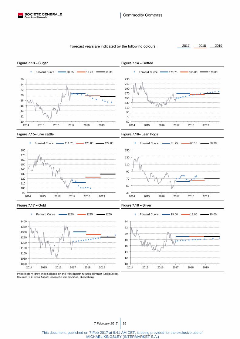
Commodity Compass

7 February 2017 35


Figure 7.13 – Sugar Figure 7.14 – Coffee

Figure 7.15– Live cattle Figure 7.16– Lean hogs

Figure 7.17 – Gold Figure 7.18 – Silver



2017 2018 2019

10

12

14

16

18

20

22

24

26

2014 2015 2016 2017 2018 2019

Forward Curv e 20.55 19.70 19.30

50

70

90

110

130

150

170

190

210

230

2014 2015 2016 2017 2018 2019

Forward Curv e 170.75 165.00 170.00

90

100

110

120

130

140

150

160

170

180

2014 2015 2016 2017 2018 2019

Forward Curv e 111.75 123.00 129.00

30

50

70

90

110

130

150

2014 2015 2016 2017 2018 2019

Forward Curv e 61.75 65.10 68.30

1000

1050

1100

1150

1200

1250

1300

1350

1400

2014 2015 2016 2017 2018 2019


10

12

14

16

18

20

22

24

2014 2015 2016 2017 2018 2019

Forward Curv e 19.00 19.00 19.00


Commodity Compass

7 February 2017 36

Global Head of Research

Brigitte Richard-Hidden

(33) 1 42 13 78 46

[email protected]

CROSS ASSET RESEARCH – COMMODITIES GROUP

Head of Commodities Research

Dr. Michael Haigh

(1) 212 278 6020

[email protected]

New York

Natural Gas Oil & Products

Breanne Dougherty

Michael Wittner

(1) 212 278 7113 (1) 212 278 6438

[email protected] [email protected]

London

Coordinator Global Technicals Metals Cross Commodity Strategy

Stephanie Aymes

Robin Bhar

Jesper Dannesboe

(44) 207 762 5898 (44) 207 762 53 84 (44) 207 762 5603 [email protected] [email protected] [email protected]

Singapore

Cross Commodity Strategy

Mark Keenan

(65) 6326 7851 [email protected]

Bangalore

Agriculture

Rajesh Singla

(91) 80 6731 8882 [email protected]


Commodity Compass

7 February 2017 37

Disclaimer

ANALYST CERTIFICATION

Each author of this research report listed on the cover hereby certifies that the views expressed in the research report accurately reflect his or her personal views, including

views about subject securities or issuers mentioned in the report, if any. No part of his or her compensation was, is or will be related, directly or indirectly to the specific

recommendations or views expressed in this report.

The analyst(s) who author research are employed by SG and its affiliates in locations, including but not limited to, Paris, London, New York, Hong Kong, Tokyo, Bangalore,

Frankfurt, Madrid, Milan, Seoul and Warsaw.

CONFLICTS OF INTEREST

This research contains the views, opinions and recommendations of Societe Generale (SG) credit research analysts and/or strategists. To the extent that this research contains

trade ideas based on macro views of economic market conditions or relative value, it may differ from the fundamental credit opinions and recommendations contained in credit

sector or company research reports and from the views and opinions of other departments of SG and its affiliates. Credit research analysts and/or strategists routinely consult

with SG sales and trading desk personnel regarding market information including, but not limited to, pricing, spread levels and trading activity of a specific fixed income

security or financial instrument, sector or other asset class. Trading desks may trade, or have traded, as principal on the basis of the research analyst(s) views and reports.

As a general matter, SG and/or its affiliates normally make a market and trade as principal in fixed income securities discussed in research reports. SG has mandatory research

policies and procedures that are reasonably designed to (i) ensure that purported facts in research reports are based on reliable information and (ii) to prevent improper

selective or tiered dissemination of research reports. In addition, research analysts receive compensation based, in part, on the quality and accuracy of their analysis, client

feedback, competitive factors and SG’s total revenues including revenues from sales and trading and investment banking.

IMPORTANT DISCLAIMER: The information herein is not intended to be an offer to buy or sell, or a solicitation of an offer to buy or sell, any securities and has been obtained

from, or is based upon, sources believed to be reliable but is not guaranteed as to accuracy or completeness. Material contained in this report satisfies the regulatory

provisions concerning independent investment research as defined in MiFID. Information concerning conflicts of interest and SG’s management of such conflicts is contained

in the SG’s Policies for Managing Conflicts of Interests in Connection with Investment Research which is available at https://www.sgmarkets.com/#compliance SG does, from

time to time, deal, trade in, profit from, hold, act as market-makers or advisers, brokers or bankers in relation to the securities, or derivatives thereof, of persons, firms or

entities mentioned in this document and may be represented on the board of such persons, firms or entities. SG does, from time to time, act as a principal trader in equities or

debt securities that may be referred to in this report and may hold equity or debt securities positions or related derivatives. Employees of SG, or individuals connected to them,

may from time to time have a position in or hold any of the investments or related investments mentioned in this document. SG is under no obligation to disclose or take

account of this document when advising or dealing with or on behalf of customers. The views of SG reflected in this document may change without notice. In addition, SG may

issue other reports that are inconsistent with, and reach different conclusions from, the information presented in this report and is under no obligation to ensure that such other

reports are brought to the attention of any recipient of this report. To the maximum extent possible at law, SG does not accept any liability whatsoever arising from the use of

the material or information contained herein. This research document is not intended for use by or targeted to retail customers. Should a retail customer obtain a copy of this

report he/she should not base his/her investment decisions solely on the basis of this document and must seek independent financial advice.

The financial instruments discussed in this report may not be suitable for all investors and investors must make their own informed decisions and seek their own advice

regarding the appropriateness of investing in financial instruments or implementing strategies discussed herein. The value of securities and financial instruments is subject to

currency exchange rate fluctuation that may have a positive or negative effect on the price of such securities or financial instruments, and investors in securities such as ADRs

effectively assume this risk. SG does not provide any tax advice. Past performance is not necessarily a guide to future performance. Estimates of future performance are

based on assumptions that may not be realized. Investments in general, and derivatives in particular, involve numerous risks, including, among others, market, counterparty

default and liquidity risk. Trading in options involves additional risks and is not suitable for all investors. An option may become worthless by its expiration date, as it is a

depreciating asset. Option ownership could result in significant loss or gain, especially for options of unhedged positions. Prior to buying or selling an option, investors must

review the "Characteristics and Risks of Standardized Options" at http://www.optionsclearing.com/about/publications/character-risks.jsp. or from your SG representative.

Analysis of option trading strategies does not consider the cost of commissions. Supporting documentation for options trading strategies is available upon request.

Notice to French Investors: This publication is issued in France by or through Societe Generale ("SG") which is authorised and supervised by the Autorité de Contrôle

Prudentiel et de Résolution (ACPR) and regulated by the Autorité des Marchés Financiers (AMF).

Notice to U.K. Investors: Societe Generale is a French credit institution (bank) authorised by the Autorité de Contrôle Prudentiel (the French Prudential Control Authority) and

the Prudential Regulation Authority and subject to limited regulation by the Financial Conduct Authority and Prudential Regulation Authority. Details about the extent of our

authorisation and regulation by the Prudential Regulation Authority, and regulation by the Financial Conduct Authority are available from us on request.

Notice to Swiss Investors: This document is provided in Switzerland by or through Societe Generale Paris, Zürich Branch, and is provided only to qualified investors as

defined in article 10 of the Swiss Collective Investment Scheme Act (“CISA”) and related provisions of the Collective Investment Scheme Ordinance and in strict compliance

with applicable Swiss law and regulations. The products mentioned in this document may not be suitable for all types of investors. This document is based on the Directives on

the Independence of Financial Research issued by the Swiss Bankers Association (SBA) in January 2008.

Notice to Polish Investors: this document has been issued in Poland by Societe Generale S.A. Oddzial w Polsce (“the Branch”) with its registered office in Warsaw (Poland) at

111 Marszałkowska St. The Branch is supervised by the Polish Financial Supervision Authority and the French ”Autorité de Contrôle Prudentiel”. This report is addressed to

financial institutions only, as defined in the Act on trading in financial instruments. The Branch certifies that this document has been elaborated with due dilligence and care.

Notice to U.S. Investors: For purposes of SEC Rule 15a-6, SG Americas Securities LLC (“SGAS”) takes responsibility for this research report. This report is intended for

institutional investors only. Any U.S. person wishing to discuss this report or effect transactions in any security discussed herein should do so with or through SGAS, a U.S.

registered broker-dealer and futures commission merchant (FCM). SGAS is a member of FINRA, NYSE and NFA. Its registered address at 245 Park Avenue, New York, NY,

10167. (212)-278-6000.

Notice to Canadian Investors: This document is for information purposes only and is intended for use by Permitted Clients, as defined under National Instrument 31-103,

Accredited Investors, as defined under National Instrument 45-106, Accredited Counterparties as defined under the Derivatives Act (Québec) and "Qualified Parties" as defined

under the ASC, BCSC, SFSC and NBSC Orders

Notice to Singapore Investors: This document is provided in Singapore by or through Societe Generale ("SG"), Singapore Branch and is provided only to accredited

investors, expert investors and institutional investors, as defined in Section 4A of the Securities and Futures Act, Cap. 289. Recipients of this document are to contact Societe

Generale, Singapore Branch in respect of any matters arising from, or in connection with, the document. If you are an accredited investor or expert investor, please be informed

that in SG's dealings with you, SG is relying on the following exemptions to the Financial Advisers Act, Cap. 110 (“FAA”): (1) the exemption in Regulation 33 of the Financial

Advisers Regulations (“FAR”), which exempts SG from complying with Section 25 of the FAA on disclosure of product information to clients; (2) the exemption set out in

Regulation 34 of the FAR, which exempts SG from complying with Section 27 of the FAA on recommendations; and (3) the exemption set out in Regulation 35 of the FAR,

which exempts SG from complying with Section 36 of the FAA on disclosure of certain interests in securities.

Notice to Hong Kong Investors: This report is distributed in Hong Kong by Societe Generale, Hong Kong Branch which is licensed by the Securities and Futures Commission

of Hong Kong under the Securities and Futures Ordinance (Chapter 571 of the Laws of Hong Kong) ("SFO"). This document does not constitute a solicitation or an offer of

securities or an invitation to the public within the meaning of the SFO. This report is to be circulated only to "professional investors" as defined in the SFO.

Notice to Japanese Investors: This publication is distributed in Japan by Societe Generale Securities Japan Limited, which is regulated by the Financial Services Agency of

Japan. This document is intended only for the Specified Investors, as defined by the Financial Instruments and Exchange Law in Japan and only for those people to whom it is

sent directly by Societe Generale Securities Japan Limited, and under no circumstances should it be forwarded to any third party. The products mentioned in this report may

not be eligible for sale in Japan and they may not be suitable for all types of investors.

Notice to Korean Investors: This report is distributed in Korea by SG Securities Korea Co., Ltd which is regulated by the Financial Supervisory Service and the Financial

Services Commission.

Notice to Australian Investors: Societe Generale is exempt from the requirement to hold an Australian financial services licence (AFSL) under the Corporations Act 2001 (Cth)

in respect of financial services, in reliance on ASIC Class Order 03/824, a copy of which may be obtained at the web site of the Australian Securities and Investments

Commission, http://www.asic.gov.au. The class order exempts financial services providers with a limited connection to Australia from the requirement to hold an AFSL where

they provide financial services only to wholesale clients in Australia on certain conditions. Financial services provided by Societe Generale may be regulated under foreign laws

and regulatory requirements, which are different from the laws applying in Australia.

Notice to Indian Investors: Societe Generale Global Solution Center Pvt. Ltd (SG GSC) is a 100% owned subsidiary of Societe Generale, which is authorised and supervised

by the Autorité de Contrôle Prudentiel et de Résolution (ACPR) and regulated by the Autorité des Marchés Financiers (AMF). Analysts employed by SG GSC do not produce

research covering securities listed on any stock exchange recognised by the Securities and Exchange Board of India (SEBI) and is not licensed by either SEBI or the Reserve

Bank of India.

http://www.sgcib.com. Copyright: The Societe Generale Group 2016. All rights reserved.

This publication may not be reproduced or redistributed in whole in part without the prior consent of SG or its affiliates.


https://www.sgmarkets.com/#compliance

http://www.optionsclearing.com/about/publications/character-risks.jsp

http://www.sgcib.com/

five facts about shale: it’s coming back, and coming back strong

News & Politics