fisher vector image representation -...
TRANSCRIPT

Fisher Vector image representation
Machine Learning and Category Representation 2013-2014
Jakob Verbeek, December 13, 2013
Course website:
http://lear.inrialpes.fr/~verbeek/MLCR.13.14

Fisher vector image representation
• An alternative to bag-of-words image representation introduced in Fisher kernels on visual vocabularies for image categorization
F. Perronnin and C. Dance, CVPR 2007.
• FV in comparison to the BoW representation
– Both FV and BoW are based on a visual vocabulary, with assignment of patches to visual words
– FV based on Mixture of Gaussian clustering of patches, BoW based on k-means clustering
– FV Extracts a larger image signature than the BoW representation for a given number of visual words

18
3
5
8
10
Fisher vector representation: Motivation
• Suppose we want to refne a given visual vocabulary
• Bag-of-word histogram stores # patches assigned to each word– Need more words to refne the representation– But this directly increases the computational cost– And leads to many empty bins: redundancy
00
2
0
0

20
35
8
10
Fisher vector representation: Motivation
• Feature vector quantization is computationally expensive • To extract visual word histogram for a new image
– Compute distance of each local descriptor to each k-means center – run-time O(NKD) : linear in
• N: nr. of feature vectors ~ 104 per image• K: nr. of clusters ~ 103 for recognition• D: nr. of dimensions ~ 102 (SIFT)
• So in total in the order of 109 multiplications
per image to obtain a histogram of size 1000
• Can this be done more efciently ?!– Yes, extract more than just a visual word histogram

20
3
5
8
10
Fisher vector representation in a nutshell
• Instead, the Fisher Vector also records the mean and variance of the points per dimension in each cell
– More information for same # visual words – Does not increase computational time signifcantly – Leads to high-dimensional feature vectors
Even when the counts are the same,
the position and variance of the points in the cell can vary

Image representation using Fisher kernels
General idea of Fischer vector representation► Fit probabilistic model to data► Represent data with derivative of data log-likelihood
“How does the data want that the model changes?”
Jaakkola & Haussler. “Exploiting generative models in discriminative classifers”, in Advances in Neural Information Processing Systems 11, 1999.
Mixture of Gaussians to model the local (SIFT) descriptors
► Defne mixing weights using the soft-max function
ensures positiveness and sum to one constraint ► Diagonal co-variance matrices
L(X ,Θ)=∑n log p(xn)p(xn)=∑k πk N (xn ;mk ,Ck)
πk=expαk
∑k 'expαk '
X={xn}n=1N
p(X ;Θ)
G(X ,Θ)=∂ log p(x ;Θ)
∂Θ

Image representation using Fisher kernels
Mixture of Gaussians to model the local (SIFT) descriptors
► The parameters of the model are ► where we use diagonal covariance matrices
Concatenate derivatives to obtain data representation
L(Θ)=∑nlog p(xn)
p(xn)=∑kπkN (xn ;mk ,Ck)
Θ={αk ,mk ,C k}k=1K
G (X ,Θ)=( ∂ L∂α1
, ... ,∂L∂αK
,∂L∂m1
, ... ,∂L∂mK
,∂ L
∂C1−1 , ... ,
∂ L∂CK
−1 )T

Image representation using Fisher kernels
Data representation
In total K(1+2D) dimensional representation,
since for each visual word / Gaussian we have
∂ L∂αk
=∑n (qnk−πk )
∂ L∂mk
=Ck−1∑n
qnk ( xn−mk )
∂ L∂C k
−1 =12∑n
qnk (C k−(xn−mk)2)
Count (1 dim) :
Mean (D dims) :
Variance (D dims) :
G(X ,Θ)=( ∂ L∂α1
, ... ,∂ L∂αK
,∂ L∂m1
, ... ,∂ L∂mK
,∂ L
∂C1−1 , ... ,
∂ L∂CK
−1 )T
qnk=p(k∣xn)=πk p(xn∣k)p(xn)
With the soft-assignments:
More/less patches assigned to visual word than usual?
Center of assigned datarelative to cluster center
Variance of assigned datarelative to cluster variance
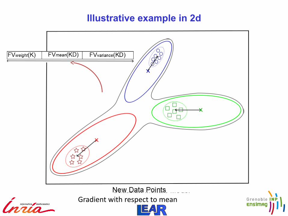
Gradient with respect to mean
Illustrative example in 2d

Function approximation view
Suppose our local descriptors are 1 dimensional for simplicity ► Vocabulary quantizes the real line
Suppose we use a linear function, eg for image classifcation ► BoW: locally constant function
► FV: locally constant + linear + quadratic function
f (x ;w)=∑k=1
Kxkwk
f (x ;w)=∑k=1K [ ∂L
∂αk∂L∂μk
∂L∂C k
−1 ]T wk
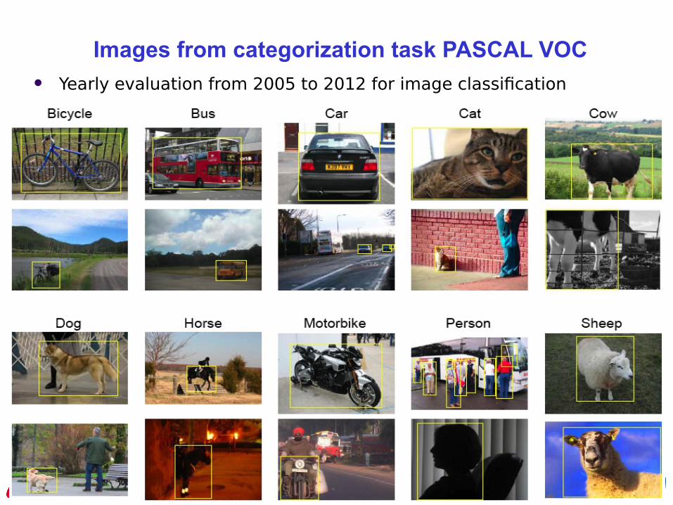
Images from categorization task PASCAL VOC Yearly evaluation from 2005 to 2012 for image classifcation

Fisher vectors: classification performance VOC'07
• Fisher vector representation yields better performance for a given number of Gaussians / visual words than Bag-of-words.
• For a fxed dimensionality Fisher vectors perform better, and are more efcient to compute

Bag-of-words vs. Fisher vector image representation
Bag-of-words image representation► Of-line: ft k-means clustering to local descriptors► Represent image with histogram of visual word counts: K dimensions
Fischer vector image representation► Of-line: ft MoG model to local descriptors ► Represent image with gradient of log-likelihood: K(2D+1) dimensions
Computational cost similar:► Both compare N descriptors to K visual words (centers / Gaussians)
Memory usage: higher for fsher vectors► Fisher vector is a factor (2D+1) larger, e.g. a factor 257 for SIFTs !
For 1000 visual words the FV has 257,000 dimensions► However, because we store more information per visual word, we can
generally obtain same or better performance with far less visual words
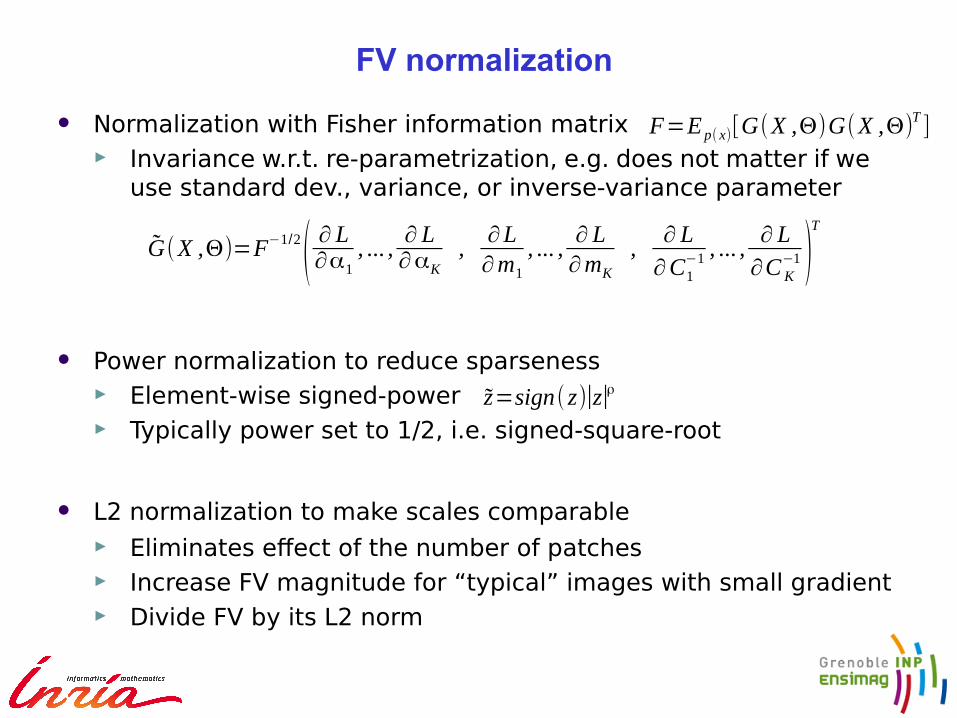
FV normalization
Normalization with Fisher information matrix► Invariance w.r.t. re-parametrization, e.g. does not matter if we
use standard dev., variance, or inverse-variance parameter
Power normalization to reduce sparseness► Element-wise signed-power► Typically power set to 1/2, i.e. signed-square-root
L2 normalization to make scales comparable► Eliminates efect of the number of patches► Increase FV magnitude for “typical” images with small gradient► Divide FV by its L2 norm
G̃(X ,Θ)=F−1/2( ∂ L∂α1
, ... ,∂ L∂αK
,∂L∂m1
, ... ,∂ L∂mK
,∂ L
∂C1−1 , ... ,
∂ L∂C K
−1 )T
F=E p( x)[G(X ,Θ)G(X ,Θ)T ]
z̃=sign( z)∣z∣ρ

FV normalization, effect on performance
Power normalization to reduce sparseness L2 normalization to make scales comparable Can also use Spatial Pyramids
► compute FV per spatial cell, and concatenate► Here: 1x1, 2x2, 3x1 grid over image, 8 cells total
Power + L2 normalization most important
Spatial Pyramid also helps, but increases FV size by a factor 8

PCA projection of local features
We used diagonal variances► Assumes dimensions are de-correlated► Not true for most local descriptors, like SIFT
Perform PCA on the descriptors to de-correlate them► Possibly also reduce the dimension too
Efect on image classifcation performance

Reading material
A recent overview article on the Fisher Vector representation
► Image Classification with the Fisher Vector: Theory and Practice
Jorge Sanchez; Florent Perronnin; Thomas Mensink; Jakob Verbeek
International Journal of Computer Vision, springer, 2013