fiscal union in europe? redistributive and stabilising ... · fiscal union in europe?...

Fiscal Union in Europe? Redistributive and

Stabilising Effects of a European Tax-Benefit

System and Fiscal Equalisation Mechanism

Olivier Bargain, Mathias Dolls, Clemens Fuest,

Dirk Neumann, Andreas Peichl, nico Pestel and

Sebastian Siegloch

Oxford University Centre for Business Taxation

Said Business School, Park End Street,

Oxford, Ox1 1HP

WP 12/22

Fiscal Union in Europe? Redistributive and Stabilising Effects

of a European Tax-Benefit System and Fiscal Equalisation

Mechanism 1

Olivier Bargain, Mathias Dolls, Clemens Fuest, Dirk Neumann,

Andreas Peichl, Nico Pestel, Sebastian Siegloch

Preliminary version of a paper prepared for the

56th Panel Meeting of Economic Policy, October 2012;

This version: September 15th, 2012

Abstract: The current debt crisis has given rise to a debate about deeper fiscal integration in

Europe. The view is widespread that moving towards a ‘fiscal union’ would have a stabilising

effect in the event of macroeconomic shocks. In this paper we study the economic effects of

introducing two elements of a fiscal union: Firstly, an EU-wide tax and transfer system and

secondly, an EU-wide system of fiscal equalisation. Using the European tax-benefit calculator

EUROMOD, we exploit representative household micro data from 11 Eurozone countries to

simulate these policy reforms and to study their effects on the distribution of income as well as

their impact on automatic fiscal stabilisers. We find that replacing one third of the national tax

and transfer systems by a European system would lead to significant redistributive effects both

within and across countries. These effects depend on income levels and the structures of the

existing national tax and transfer systems. The EU system would improve fiscal stabilisation

especially in credit constrained countries. It would absorb between 10 and 15 per cent of a

macroeconomic income shock. Introducing a fiscal equalisation system based on taxing capacity

would redistribute revenues from high to low income countries. The stabilisation properties of

this system, however, are ambiguous. This suggests that not all forms of fiscal integration will

improve macroeconomic stability in the Eurozone.

JEL codes: H2, H3, J22

Keywords: European income tax, automatic stabilisation, fiscal union

1 Bargain ([email protected]) is affiliated to Aix-Marseille School of Economics, IZA and CEPS/INSTEAD, Fuest ([email protected]) to University of Oxford, University of Cologne, CESifo and IZA, Dolls ([email protected]), Neumann ([email protected]), Pestel ([email protected]) and Siegloch ([email protected]) to IZA and University of Cologne and Peichl ([email protected]) to IZA, University of Cologne, ISER and CESifo. This paper uses EUROMOD version D16. Here, the ECHP and EU-SILC were made available by Eurostat; the Austrian version of the ECHP by Statistik Austria; the PSBH by the University of Liège and the University of Antwerp; the IDS by Statistics Finland; the EBF by INSEE; the GSOEP by DIW Berlin; the Living in Ireland Survey by the ESRI; the SEP by Statistics Netherlands; the Greek HBS by the National Statistical Service; the SHIW by the Bank of Italy and the EBF by INSEE. None of the institutions cited above bear any responsibility for the analysis or interpretation of the data reported here. Peichl is grateful for financial support by Deutsche Forschungsgemeinschaft DFG (PE1675). We would like to thank Koen Decancq, Frank Vandenbroucke, the editor, Nicola Fuchs-Schündeln, three anonymous referees as well as seminar and conference participants in Antwerp (CSB), Berlin (ESMT), Bonn (IZA), Dresden (IIPF), Dublin (IMA), Göttingen (VfS) and Mannheim (ZEW) for useful comments and suggestions. We are indebted to all past and current members of the EUROMOD consortium for the construction and development of EUROMOD. The usual disclaimer applies.

1

1 Introduction

The process of European unification, which started with the creation of the European Coal and

Steel Community in 1951, has slowly but surely moved into the direction of increasing economic

and political integration. The creation of a customs union and a common market followed, and

the adoption of a single currency in the European Monetary Union (EMU) in 1999 was the latest

major step (Sapir, 2011). But EMU is unlikely to be the final step. Proponents of deeper political

integration in Europe have repeatedly argued that the European Union (EU) needs a larger

budget and the right to levy taxes. For instance, Sijbren Cnossen argues in favour of “a federal

government with real taxing powers and financial leverage over the Member States to mitigate

adverse effects that might arise from Member State tax policies” (Cnossen, 2001, p. 466f). Lambert

(2011) goes even further and develops a normative concept of an equitable EU tax redistribution

system.

Until recently the idea of introducing federal fiscal structures in the EU was mostly discussed in

academic circles and think tanks but played only a minor role in the policy debate. However, the

current debt crisis in the Eurozone has brought the idea of deeper fiscal integration to the top of

the European policy agenda. Many observers argue that the currency union cannot survive

unless it is complemented by a ‘fiscal union’. The concept of creating a fiscal union has many

interpretations, ranging from the rather limited approach of introducing a set of balanced

budget rules to the more ambitious project of creating a federal government with significant tax

and spending powers comparable to existing federations like the US (see e.g. Bordo et al., 2011,

Fuest and Peichl, 2012).

While deeper fiscal integration in Europe is thus a widely debated issue, little is known about its

economic implications. This paper contributes to filling this gap by analysing the economic

effects of two key elements of fiscal integration, i) the introduction of an EU-wide integrated tax

and transfer system which partly or fully replaces the existing national systems and ii) the

introduction of a system of fiscal equalisation. These reforms would be far reaching, but they do

reflect the widespread view that radical steps towards more fiscal integration are necessary to

improve the stability of the Eurozone. Even if these reforms seem unlikely to find political

support in the short term, it is important to understand why this might be the case and whether

much is lost if fiscal integration fails to proceed into this direction. Our analysis includes 11

Eurozone countries.2 We employ the European tax-benefit calculator EUROMOD which uses

harmonised and representative household micro data and allows calculating taxes, transfers and

disposable incomes for each household type and country. EUROMOD allows us to run

counterfactual simulations so that we can analyse policy reforms and their effects on tax

revenues, the income distribution and labour supply. We proceed as follows. First, we construct

2 These are the founding members of the EMU (except Luxemburg) and include Austria, Belgium, Finland, France,

Germany, Greece, Ireland, Italy, the Netherlands, Portugal and Spain. In the following we will refer to this group as ‘the

EU’, neglecting that the European Union has 27 member countries. We focus on these 11 countries because of data

availability and because we are primarily interested in studying fiscal integration in the Eurozone.

2

a European tax and transfer system, which can be interpreted as an average of the national tax

and transfer systems. The system is designed such that it generates the same net revenue on the

EU level but not necessarily at the level of each member state. Second, we consider various

scenarios where the European tax and transfer system (fully or partly) replaces the national

systems. In the first scenario, we assume that the national tax and transfer systems are reduced

by one third and this gap is filled by the European system. In other scenarios we look at a full

substitution of the national systems and at a more progressive European system.

Regarding the economic impact of these reforms, we focus on two issues. Firstly, we consider the

distributional effects of the reform scenarios, which are of key importance for the political

feasibility of fiscal integration. The reforms lead to a redistribution of tax burdens between

member states and across individuals, where some member states benefit and others lose.

Within member states, households at different income levels can be affected very differently. We

measure the redistributive effects taking into account behavioural responses in the form of

labour supply adjustments (Bargain et al., 2012).3

Secondly, we are interested in the impact of the different reforms on the ability of the tax and

transfer system to act as an automatic stabiliser in the presence of macroeconomic shocks. This

aspect is highly relevant for the debate on the role of fiscal integration for the future of the

Eurozone. In particular, fiscal integration is expected to improve the resilience of the Eurozone

in the event of asymmetric shocks. Building on Dolls et al. (2012), we study simulated shocks on

gross income and we investigate to which extent the existence of the European tax and transfer

system contributes to macroeconomic stabilisation. We are especially interested in a scenario

where individual countries are unable to let automatic stabilisers of the national tax and transfer

system work because they cannot borrow. In this case the automatic stabilisers of the European

tax and transfer system are of key importance.

Our analysis leads to the following results. The introduction of a European tax and transfer

system which replaces one third of the national systems would increase the disposable income

of a small majority of households in Europe. At the same time it would lead to significant

redistribution between countries. The winners include Greece, Portugal, Spain, Italy and,

surprisingly, Germany. The average gains range between roughly 8 per cent of disposable

income in Greece and one per cent in Germany. The gains in the southern European countries

come at the cost, however, of a decline in labour supply. Austria, France, Ireland and the

Netherlands lose on average. The finding that Germany benefits, is surprising, because

intuitively, one would expect gains and losses to be driven by differences in income levels

between countries. This is true up to a point, but the structure of the existing tax and transfer

systems plays a role as well. In France, for instance, average per capita income is lower than in

Germany but the national tax and transfer system is less progressive than the German one and

relies more on indirect taxes than on income taxes. Within countries, households at different

3 Note that the simulation model we are using assumes full benefit take-up and no tax evasion. In addition, other

margins of adjustment than labor supply cannot be captured. This includes, but is not limited to, tax evasion or

avoidance and income shifting. The implications of relaxing these assumptions will be discussed further below.

3

income levels are affected differently. In the southern European countries, the gains are

concentrated among the low income quintiles. In high income countries, the high income

quintiles gain on average. The middle class loses in many countries. We also analyse the impact

of the reform on income inequality. Overall, introducing the EU tax system reduces EU-wide

income inequality. In most cases, this also holds for inequality within countries. In sum however,

these findings cast doubts on the political feasibility of the reform under consideration. While a

small majority of EU citizens would gain, this is not true for a majority of countries. We analyse

the implications considering current and prospective voting mechanisms of the Council of the

European Union.

How does the introduction of the EU tax-benefit system affect automatic fiscal stabilisers?

Unsurprisingly, the reform will increase automatic stabilisers in countries where the national tax

systems have smaller stabilisers compared to the European average – this applies in particular

to the southern European countries. A key question is by how much the EU tax and transfer

system contributes to overall fiscal stabilisation. In the case where the EU tax and transfer

system replaces one third of the national system, the EU system would absorb between 10 per

cent (Ireland) and 15 per cent (Germany) of a shock to gross income. In the case of the more

progressive EU tax system, the stabilisation properties remain similar.

Finally, what are the implications of introducing a system of fiscal equalisation, rather than a

common tax and transfer system? Note that with this scenario, the national tax and transfer

systems stay in place and tax revenues are now redistributed across countries. The fiscal

equalisation system we consider compensates countries for differences between their national

and the EU average taxing capacity. As those differences are fully equalised, the redistributive

effects are considerable. As one would expect, the system implies transfers flowing from high to

low income countries.

How does this system of fiscal equalisation perform when it comes to providing stabilisation in

the event of an asymmetric shock? We consider a shock in the form of a decline in gross income

by 5 per cent which hits Greece, Italy, Spain, Portugal and Ireland (the ‘GIIPS’ group). In all other

countries, income remains constant. Interestingly, in terms of the stabilisation effects it offers,

the fiscal equalisation mechanism performs rather poorly. In Greece, fiscal equalisation even

leads to a destabilising effect. In Portugal, the stabilisation effect is close to zero. The reason is

that, in the situation before the shock, Greece and Portugal are the countries which benefit most

from fiscal equalisation. The shock reduces their taxing capacity, but it also reduces the taxing

capacity of the union as a whole. Since other large countries like Spain and Italy and even a net

contributor (Ireland) are affected, the sum of money available for fiscal equalisation declines,

and countries which benefited initially may even lose transfers. Those findings become even

more prevalent when simulating a shock comparable to the 2008-09 recession which has hit not

just a few but all countries under analysis.

Our findings have important policy implications. In order to achieve significant income

stabilisation through the introduction of an EU tax and transfer system, the magnitude of the

simulated system would have to be considerable. Replacing one third of the national systems by

a European system would lead to stabilisers absorbing between 10 and 15 per cent of a

4

macroeconomic shock. But establishing such a system would give rise to significant

redistributive effects, which will make political acceptance difficult.

The alternative of setting up a fiscal equalisation system could give rise to even larger

redistributive effects, depending on the design of the system. But a high degree of fiscal

equalisation does not imply that the system always offers a high degree of fiscal stabilisation in

the presence of asymmetric shocks. The stabilisation effect may be different for different

countries, and the example considered here shows that even a destabilising effect is possible.

The setup of the rest of this paper is as follows. Section 2 describes the related literature and the

concept and design of a fiscal union in our simulation scenarios. Section 3 introduces the

empirical strategy, i.e. the micro data and the tax-benefit calculator EUROMOD, the different

scenarios as well as some descriptive information. The results are presented in Section 4.

Section 5 concludes.

2 Conceptual framework and related literature

2.1 Related literature

The related literature about European integration in the area of fiscal policy can be divided into

two broad areas.4 The first strand of literature focuses on the EU budget, its expenditure and its

revenue sources. This literature discusses issues like the size and structure of the EU budget as

well as its current revenue sources (see, e.g., Atkinson, 2002; Begg, 2005). One important issue is

whether the EU should be allowed to levy taxes. Currently the EU is essentially financed through

contributions from the member states. Most of the literature about EU taxes focuses on indirect

taxes like a European VAT or an environmental tax. Other proposals include a European

corporate income tax or, more recently, a European financial transactions tax (see e.g. Le

Cacheux, 2007, Begg, 2011). In this literature the key arguments in favour of a European tax are

that such a tax would increase the transparency and improve democratic control of EU policies.

Wigger and Wartha (2003) take a different approach and develop a theoretical model which

focuses on the interaction between tax coordination and the allocation of taxing rights between

the national and the EU level. They argue that, in the presence of tax coordination between

member states, giving the EU the power to tax is not desirable because the coexistence of taxing

powers at the national and the EU level will lead to overtaxation.

The key difference of this literature to the present paper is that none of these contributions

looks at the quantitative economic effects of introducing a European tax while our focus is on the

quantitative effects in terms of redistribution, labour supply, and macroeconomic stabilisation.

The second strand of literature related to the present paper is the large body of work on the

implications of EMU for fiscal policy integration. An important early discussion of the key issues

4 There is a third strand of literature which discusses the coordination and harmonisation of taxes and tariffs required

to create a common market. This literature is surveyed, for instance, in Keen (1993). For the present paper this

literature is less relevant because our focus is not on tax obstacles for border crossing economic activity.

5

can be found in the MacDougall Report (1977), which had the broad objective to analyse the role

of public finances for European integration. One of the key findings of the report is that “public

finance in existing economic unions plays a major role in cushioning short term and cyclical

fluctuations ... there is no such mechanism in place ... between member countries and this is an

important reason why in present circumstances monetary union is impracticable” (p.12). This

view has been confirmed by most of the later literature on the implications of EMU for fiscal

policy in Europe. Eichengreen (1990) compares Europe to the US and emphasises that the

federal income tax in the US provides significant insurance against asymmetric macroeconomic

shocks. He argues that, since regional problems are likely to be greater in Europe than in the US,

fiscal shock absorbers would have to be significantly larger.

Along similar lines, many economists have warned that the Euro area is too heterogeneous and

thus far away from being an optimum currency area along the lines of Mundell (1961) and

Kenen (1969). Therefore, the EMU will be fragile and vulnerable to economic shocks unless it is

complemented by more fiscal integration (see e.g. Sala-i-Martin and Sachs, 1992; Buiter et al.,

1993; Masson, 1996; Eichengreen and Wyplosz, 1998; Engwerda et al., 2002; Uhlig, 2003).

Several authors have proposed an increase in the European budget in order to establish a

horizontal fiscal equalisation mechanism (Italiener and Vanheukelen, 1993; Hammond and von

Hagen, 1998; Dullien and Schwarzer, 2005; Marzinotto et al., 2011). Schuknecht et al. (2011)

emphasise fiscal discipline and propose an independent fiscal council for the Euro area with the

aim to improve governance and compliance.

Some economists have taken the opposite view and argue that the ‘unprecedented divorce

between the main monetary and fiscal authorities’ (Goodhart, 1998) also has advantages because

it limits political influence on monetary policy (e.g. Beetsma and Bovenberg, 1998; Dixit and

Lambertini, 2003; Beetsma and Giuliodori, 2010). However, the current debt crisis in the

Eurozone has renewed doubts about the wisdom of this construct. Today, the view seems to

prevail that a monetary union like the EMU cannot work without a major policy shift towards a

fiscal union.

2.2 What is a ‘fiscal union’? Simulation scenarios

In the debate on reforms of fiscal institutions in the Eurozone, it is not always clear what exactly

the term ‘fiscal union’ is supposed to mean and different people use it very differently. Fuest and

Peichl (2012) suggest five possible elements of a European fiscal union. These are (i) fiscal rules

for the member states as well as rules concerning policy coordination and supervision, (ii) a

crisis resolution mechanism, (iii) a joint guarantee for government debt, (iv) a fiscal equalisation

and/or other mechanisms for transfers between countries and (v) an extended EU budget and

European taxes.

While much of the current political debate focuses on short term crisis management and

therefore emphasises elements (i) - (iii), the focus of this paper is on elements (iv) and (v),

which are more relevant in the long term.

Of course, a significant shift of policy responsibilities to the European level raises many

questions in terms of construction and how the central budget is used. More precisely, one key

6

question is how the fiscal equalisation mechanism combined with a European income tax will

function. In order to choose scenarios for the type of a fiscal union we are going to model, we

distinguish three dimensions which serve as a framework for the specific design of a European

tax-benefit system: (1) overall revenue, (2) the design of the EU tax and transfer system and its

share in overall taxes and transfers and (3) the assignment of revenues and the existence of a

fiscal equalisation mechanism.

First, for overall revenue, we assume our reforms to be revenue neutral at the EU level. This

choice appears to be a natural solution for two reasons. First, it ensures the comparability of

different scenarios. Second, by keeping the overall budget constant, we avoid the debate about

increasing (decreasing) the size of government. This, however, does not imply revenue

neutrality at the national level, as will be discussed further below.

Second, for the design of the EU tax-benefit system, several approaches are possible in principle.

The system could be designed from scratch. A simple way of doing so would be to introduce an

EU tax surcharge, where the surcharge could simply be a percentage of national income tax

payments. But this approach raises various difficulties. Most importantly, since national income

tax systems differ widely across member states, such a system would benefit countries with low

income taxes, and it would create incentives for individual member states to rely more on

revenue sources other than income taxes like e.g. social insurance contributions or replace

transfers by tax credits which reduce income taxation.

Therefore, we consider the introduction of a separate tax and transfer system which would

partly or fully replace the national systems. What we will use here is an ‘average system’ which

leads to the same revenue and progressivity at the EU level as a combination of the existing

national systems. At least with view to progressivity, this is an arbitrary choice even when

conditioning on revenue neutrality. Thus, we will also consider a scenario that increases

progressivity of the overall system, while again ensuring that overall revenue remains constant.

Regarding the share of the EU system in overall taxes and transfers, a wide range of scenarios

could be considered. At one extreme, we could assume that the EU tax-benefit system completely

replaces national systems. However, in most existing fiscal unions, there are tax-benefit systems

at different levels of government. For instance, in the US, two thirds of overall tax revenue are

collected at the federal level versus one third at the state and local level. However, moving two

thirds of the national tax and transfer systems to the EU level seems implausible. In our analysis,

we will therefore look at two scenarios: in the first scenario the EU system replaces one third of

the national systems; in the second scenario, the national systems are replaced entirely. Clearly,

the latter scenario is more relevant as a theoretical benchmark whereas the former might be

something that might happen if the EU decides to move to a federal fiscal system.

Third, we have to make assumptions regarding the assignment of tax revenues and the existence

of a fiscal equalisation mechanism. We do this as follows. In our simulations of the introduction

of a European tax and transfer system, we assume that any net revenues (revenues after taxes

and transfers) generated by the EU system will be pooled, and each country will receive a

transfer from this pool which is equal to the initial net revenue collected under the national tax

systems. This assumption implies that redistribution between countries in our simulations is

7

driven by the fact that the EU average system changes the net tax burdens of households. We

hold constant the net tax revenue each member state receives, so that the provision of public

goods is kept constant in all countries, as are budget deficits. An alternative assumption would

be to assume that net tax revenues are redistributed as well.

This issue will be discussed in the simulations about fiscal equalisation. For this purpose we will

assume that member states keep their tax and transfer systems but the EU average tax and

transfer system will be used as an indicator of taxing capacity. Member states with a taxing

capacity below the EU average will be recipients in the fiscal equalisation mechanism and vice

versa. We will then investigate to which extent i) the fiscal equalisation mechanism redistributes

income between member states compared to a situation without equalisation and ii) the fiscal

equalisation mechanism cushions the impact of an asymmetric economic shock.

2.3 Conceptual framework

In this section we describe the income concept used in our simulations, we illustrate the idea of

constructing an average tax system with a simple example and we explain how our simulations

deal with government budget constraints. Our simulations proceed as follows. We start with

representative micro data from each of the 11 EU member states which enter our simulations.

Gross market income �� of individual i is defined as the sum of all incomes from market

activities:

�� = �� + �� + �� + �� +�, (1)

where �� is labour income, �� business income, �� capital income, �� property income, and � other income. Disposable income � is defined as market income minus net government

intervention �� = � �� + �� +�� :

� = �� − �� = �� − (� �� + �� − ��), (2)

where � �� are direct taxes, �� employee social insurance contributions, and �� are cash

benefits (i.e. negative taxes). Note that, due to a lack of micro data, we cannot include indirect

taxes and in-kind benefits in our analysis. In the following, we refer to the difference between

taxes and social insurance contributions paid and transfers received as net taxes.

For an illustrative example of a common tax and transfer system, assume two countries A and B

with individual net tax schedules �� = ��(��). To keep the example as simple as possible,

consider a linear progressive net tax schedule independent of characteristics �� , i.e. �� =��(��) = �� − �� with �� the marginal tax rate and �� a refundable tax credit (equal to a benefit

if �� is negative). A simple way to introduce a revenue neutral common tax system is to use the

average system

�� = �� !�"�#�� !#$ = ��"�#

$ �� − !�"!#$ , (3)

i.e. applying the average marginal tax rate and tax credit. In reality, tax-benefit systems do not

only depend on income but on other characteristics, too. In addition, the observed tax-benefit

systems are directly progressive. We therefore construct the EU average tax and transfer system

8

using a regression approach as described in section 3.2, but the economic intuition is as in our

simple example.

How do we take into account the government budget constraints in our simulations? Assume

that country A has �� citizens with characteristics (��, &�), and country B has �' citizens with

characteristics (�', &'). Under the national tax and transfer systems, the national government

budget constraint of country k (k=A,B) in period t is given by

∑ ��*�+,-./ + �*�0 − �*� = �*� (4)

where ∑ �-*�1-./ is revenue from ‘net taxes’ (income taxes and social insurance contributions net

of transfers), �*�0 is revenue from other taxes like consumption taxes or corporate income taxes,

�*�is the budget deficit and �*� is public expenditure excluding transfers. This would include

spending on defence, infrastructure, police, education and other public services, but also interest

payments on government debt.

In the following, we omit the time index t to keep the notation simple. Equations (4) holds in the

reference scenario in our simulations – a scenario with no supranational tax and transfer

system. In this reference scenario the aggregate disposable income of the citizens of country k

(k=A,B) is given by

∑ �* = ∑ (��* − ��*+,�./

+,�./ ). (5)

Now assume that both countries form a union and define a common tax and transfer system

denoted by �34 = �34(�, 5). In the following, we denote by ��34* the net tax payment that arises

if the common tax system is applied to citizen i residing in country k (k=A,B). This tax system is

constructed so that, for the union as a whole, and for given market incomes, it generates the

same net tax revenue as the national tax systems:∑ �� + ∑ �-' = ∑ ��34� + ∑ �-34'+#-./

+��./

+#-./

+��./ .

In the next step, countries A and B reduce their national net taxes by a factor 1 − 7 and fill the

gap by introducing the common tax system. As a result aggregate disposable income of the

citizens of country k (k=A,B), becomes ∑ �* = ∑ (��* − (1 − 7)��* − 7��34*)+,-./

+,�./ .

So far, we have assumed that market incomes remain constant. But the reform of the tax and

transfer system will affect market incomes because it affects labour supply. Denote the market

income of individual i residing in country k before the reform by ��*8 and market income after the

reform by ��*/ . Then the change in aggregate disposable income of citizens of country k,

∑ [�*/ − �*8+,-./ ] can be expressed as

∑ [�*/ − �*8+,�./ ] = ∑ [��*/ − ��*8 − [(1 − 7)�*;��*/ , 5<=> − 7�34;��*/ , 5<=> − �*;��*8 , 5<=>]]+,

�./ (6)

In our analysis, we focus on the change in disposable income as an indicator of whether

countries or individuals benefit or lose from a reform.5 What are the factors driving changes in

5 Here one may object that welfare should be used as an indicator because more labour supply may increase

disposable income but not welfare. We use disposable income because this is a widespread and easily understandable

9

disposable income in different countries? Firstly, countries where the national tax and transfer

system implies a low net tax burden compared to the European average will suffer a loss in

disposable income as a result of the reform simply because European taxes are higher. Secondly,

low income countries will tend to experience an increase in disposable incomes because they

benefit from the fact that they now share a tax and transfer system with richer taxpayers in

other countries. Thirdly, changes in disposable income will occur as taxpayers adjust their

labour supply.

How does the reform affect overall tax revenue and the budget constraints of the national

governments? Consider first the impact on the national budgets. National net tax revenue

changes for two reasons. Firstly, the national tax and transfer system is cut by a factor 1 − 7.

Secondly, the net revenue generated by what remains of the national system changes due to

labour supply adjustments. The change in net tax revenue collected by country k due to the

reform is given by

∑ [��*/ − ��*8+,�./ ] = ∑ [(1 − 7)�*;��*/ , 5<=> − �*;��*8 , 5<=>]+,

�./ (7)

The net revenue collected by the common tax system, which we denote by ?34, is given by

?34 = 7[∑ �34;��/ , 5<@>+��./ +∑ �34;�-'/ , 5AB>]+#

-./ . (8)

This net tax revenue collected at the European level is equal to the net revenue the national

governments lose by abolishing a share 7 of their national tax and transfer systems if market

income is constant. The reason is that the new tax system was designed to assure revenue

neutrality ex ante, before labour supply adjustments. Without changes in labour supply, the tax

revenue collected at the European level would be exactly sufficient to compensate the

governments of the member states for their net tax revenue losses (or gains). No further

adjustments to balance the government budgets would be required: The variables ‘other’ taxes

(�0), the budget deficits (B) and expenditures on public services (E) could be the same before

and after the reform

But since we do take into account changes in labour supply caused by the reform, revenue

neutrality ex post is not guaranteed. The net revenue collected by the common tax system may

differ from the revenue required to compensate the national governments for the changes in

their net tax revenue. Assume that the European budget nevertheless compensates the national

governments for the changes in national net tax revenue caused by the reform, after labour

supply adjustments. In this case, the European budget constraint can be written as

�34 = ∑ [��/ − ��8+��./ ] + ∑ [��'/ − ��'8+#

-./ ] − ?34 (9)

where �34 is the deficit (or, if negative, surplus) in the EU level budget. A deficit �34 > 0 arises

in the European budget if the reform leads to behavioural adjustments which reduce EU-wide

net tax revenue. In contrast, if EU-wide net tax revenue increases, the EU budget would be in

indicator, but we will also report results for welfare changes as well as disposable income changes without labour

supply adjustments. The pattern of the results is the same for all indicators.

10

surplus. If there is a deficit, the question arises how that deficit is financed and how the burden

is distributed across countries. Likewise, if there is a surplus, this money can be distributed to

the national governments. As we will show in the simulations, this effect is quantitatively so

small that it can be neglected.6

3 Empirical strategy

3.1 EUROMOD: model and database

In order to analyse the hypothetical introduction of a EU-wide tax-benefit system, we need to

run counterfactual simulations. We use the microsimulation technique to calculate taxes,

benefits and disposable income under different scenarios for a representative micro-data

sample of households. Simulation analysis allows conducting a controlled experiment by

changing the parameters of interest while holding everything else constant. Therefore, the

researcher does not have to deal with endogeneity problems when identifying the effects of the

policy reform under consideration.

Simulations are carried out using EUROMOD, a static tax-benefit model for the EU countries,

which was designed for comparative analysis. Through a common framework, which has a

greater flexibility than typical national models to accommodate a range of different tax-benefit

systems, it allows the comparison of countries in a consistent way. EUROMOD was originally

created in the late 1990s, by a consortium of research institutions from each EU15 country with

a good knowledge and expertise in their respective national tax-benefit systems. The tax-benefit

systems included in the model (1998 and 2001 for the EU-15, 2003 for a subset of countries and

2005 for four new member states) have been validated against aggregated administrative

statistics as well as national tax-benefit models (where available), and the robustness has been

checked through numerous applications (see, e.g., Bargain, 2007).

The model can simulate most direct taxes (especially income taxes on all sources of income

including tax credits, payroll taxes and social insurance contributions) and benefits (e.g., welfare

benefits and social assistance, housing benefits, family and child benefits) except those based on

previous contributions as this information is usually not available from the cross-sectional

survey data used as input datasets. Information on these instruments is taken directly from the

original data sources. While simulations are usually carried out for counterfactual situations,

EUROMOD also simulates various taxes and transfers for the baseline that are not observed in

the original data.

Information on consumption is missing in the data; hence indirect taxes as well as taxes on

corporate profits are not included in the model. The same is true for in-kind benefits. Clearly,

6 In the different scenarios the deviations from revenue neutrality range between a surplus of 0.44 Euros per

household and week to a deficit of 0.64 Euros per week. Table C2 in the appendix reports these numbers as a

percentage of net tax payments.

11

these elements differ between countries and affect the results presented. Table A.1 in the

Appendix reports the shares of taxes which are captured by the model for the different

countries. Clearly, these shares vary across countries - between 44 per cent (Ireland, Portugal)

and 66 per cent (Germany). We do not find a systematic relationship between these shares and

our results. In addition, the table contains information about the deficit and debt ratios for each

country. In our analysis we do not impose a balanced budget rule and hence keep these initial

conditions fixed.

EUROMOD assumes full benefit take-up and tax compliance, focusing on the intended effects of

tax-benefit systems, which may influence the results in terms of the redistributive and

stabilizing effects of fiscal reforms when this behaviour varies substantially across countries.

The main stages of the simulations are the following. First, a representative micro-data sample

of individuals in households (including information on gross income from various sources as

well as demographic characteristics which are relevant to determine taxes and benefits such as

household size, age and number of children, marital status, employment status, disability status,

region of living; see also below) and the respective tax-benefit rules (e.g. for singles or couples)

are read into the model. Then for each tax and benefit instrument, the model constructs

corresponding assessment units (for instance the individual, family or household), ascertains

which are eligible for that instrument and determines the amount of benefit or tax liability for

each member of the unit (for instance accounting for the individual or joint assessment of taxes

or benefits for each household member). Finally, after all taxes and benefits are simulated,

disposable income is calculated. This simulated disposable income includes all monetary

incomes, except capital gains and irregular incomes.7

Due to data limitations, our analysis is based on the 2001 tax-benefit systems, two years after

the introduction of the Euro for the EURO-12 countries.8 This is important to keep in mind,

especially given that many countries implemented significant reforms in their tax and transfer

systems in the last decade. The input datasets for these countries are summarised in Table A.2 in

the Appendix. The sample sizes vary across countries from 7,000 to more than 25,000

households. All monetary variables are updated to the 2001 year using country-specific uprating

factors, as the income reference period varies from 1999 to 2001.

3.2 Scenarios

In this section we explain in a more technical manner how we conduct the simulations of the

different reform scenarios introduced in Section 2.2. We proceed in four steps.

7 For further information on EUROMOD, see Sutherland (2007). There are also country reports available with detailed

information on the modelling and validation of each tax benefit system, see

http://www.iser.essex.ac.uk/research/euromod.

8 Unfortunately, this is the most recent year for which all countries and data is available. For later years, Germany and

France would be missing. At the time of writing this paper, a more recent version of Euromod for the EU-27 countries

is being constructed.

12

1. We use EUROMOD, which contains an exact representation of the (direct) tax-benefit

systems of the Eurozone countries in 2001, to extract net taxes for each individual (and

household) i in representative samples for each country c. In particular, EUROMOD

simulates the country specific net taxes (income and payroll taxes minus benefits)

��E = �E(��) as a function of gross market income �� and a vector of non-income factors

�� (e.g. marital status, number and age of children) taken from the data.

2. Using those simulated net taxes ��E for all European citizens, we obtain the average EU

tax function ��,34!�� such that it yields the same net revenue at the EU level as the sum of

the national systems. In order to calculate this average system, we adopt a regression

approach and estimate the following reduced form tax function on the pooled sample:

��E = F��34(��) + G�. (10)

Function �34 is specified as a flexible transformation of (��) → ��E. G� is the OLS

residual and F� the household sample weight. We use a very flexible functional form with

higher order polynomials and interaction terms of income and basically all

characteristics observed in the data which are relevant for taxes and benefits (such as

gross income from various sources, household size, age and number of children, marital

status, employment status, disability status, region of living). Table A.3 in the Appendix

reports the mean values of the main variables in each country. Given that weights sum

up to the EU population size this function directly accounts for a population weighted

average tax function at the EU level. The fit of this tax regression in terms of the R2-

measure is close to 1. It is not equal to 1, though, because by regressing on the pooled

sample, differences across countries will be explicitly captured, which is exactly the

differences we need to keep for the average system.

3. The estimated function is then used to predict net tax payments for the EU average tax

system ��,34!�� for each individual and household in the sample.

4. Next, we use the predicted EU average tax system to construct different scenarios of

replacing the national tax-benefit systems with an EU-wide system (again, yielding the

same revenue on the EU-level, but not for each country). In principle, a continuum of

scenarios for introducing a fiscal union is possible. We focus on two different tax

systems. We either replace the current national systems �1!� with the EU average system

�34!�� or with a system ��,34!��_J with increased progressivity compared to ��,34!��

(again yielding revenue neutrality).9 The latter scenario can be seen as a proxy for a

switch towards a more “Northern” European system with higher progressivity. For both

9 Precisely, we calculate ��K�LM_N by first introducing a proportional surcharge of 7.5% to ��K�LMwhich subsequently

will be fully redistributed across all households in the pooled sample via a lump sum transfer equal to its mean value

across households, i.e. ��,34!��_J = ��,34!�� + ��,34!�� ∗ 0.075 − R with R = /+∑ ��,34!��+

�./ ∗ 0.075 Results for a

surcharge of 5% (10%) are qualitatively in line with the results presented here and simply less (more) pronounced

with view to the expected effects when increasing progressivity for the EU average system (detailed results available

upon request).

13

systems, we simulate two different weighted combinations of the current national

system and the EU average system resulting in a total of four different scenarios. Here,

we simply look at full integration (the share of the average system is 100%) and a partial

integration (which could be seen as a first step for such a major reform) of 33%. The

benchmark is the current national system of each country (i.e. the share of the average

system is 0%). Formally, we calculate for each household i of country c

�� = S��,34!�� + (1 − S)��E;S ∈ V/W , 1X.10

(11)

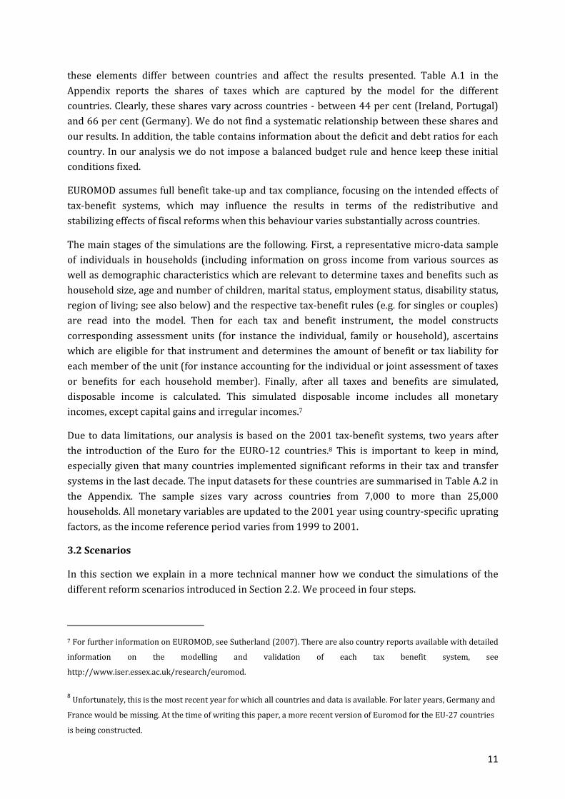
Subsequently, the four scenarios are labelled EUavg-Sc. 1, Sc. 2 and EUavg_p-Sc. 1, Sc. 2. Figure 1

plots the current national tax-benefit function as well as the two EU average functions. While the

EU average function is, by construction, basically identical to the average of the national systems,

the increased progressivity for the second function becomes visible especially at the top of the

distribution.

Fig. 1: EU average tax-benefit schemes and average of national systems

What are the general implications of this approach with view to the resulting new tax-transfer

systems of the different countries? By construction and as described in Section 2.3, we assume

that all of the revenue collected from �34!�� as well as �34!��_J goes to the central EU budget

(which remains unchanged) and is immediately redistributed across countries and households

(note that the tax function based on the pooled sample predicts household net tax payments as a

fraction of the central budget, not as a fraction of national budgets). The structure of national

10 ForS = $W, results are qualitatively similar and lie in between the results for S = /

Wand S = 1. We thus do not report

these results due to lack of space.

-.2

0.2

.4.6

net t

axes

0 .5 1 1.5gross income

T EUavg

T EUavg with increased progressivity

T nat average

Note: Based on overall means for gross income deciles; weekly thousand 2001 EUR.

Source: Own calculations based on EUROMOD.

14

budgets is affected in the sense that the importance of the simulated elements is reduced

according to the weighting factor (1 − S). In the extreme scenario with S = 1 it is decreased to

zero and fully replaced by the EU system. This leads to redistribution of (simulated) net tax

revenues between countries. This also implies that revenues and expenditures which are not

captured by our data – like revenues from indirect or corporate income taxes or expenditures on

defence and other publicly provided goods, as well as deficit (or surplus) levels – remain

constant for each country. Especially the absence of a balanced budget in the analysis is

important since, following the recent crisis, fiscal consolidation and the size of governments

have become central to the debate on fiscal reforms in Europe.11 In principle, countries with a

deficit (surplus) would need to raise more (less) revenue – or spend less (more) on benefits –

and hence the households in those countries would, c.p., lose (gain) in terms of disposable

income.

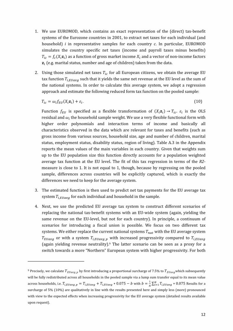
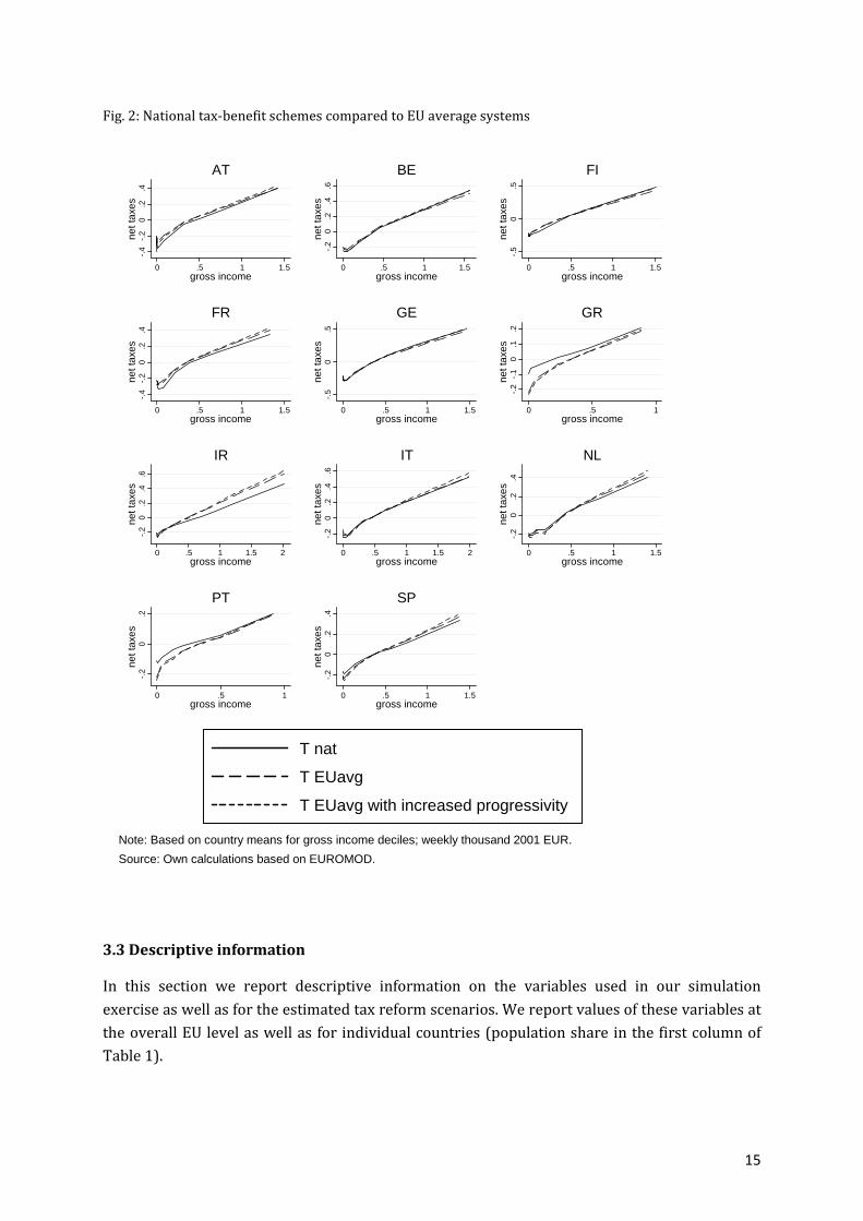
Figure 2 includes plots of the current national tax-benefit functions as well as the two EU

average functions for each country in the sample. It is immediately evident that the

redistributive effects of the different reforms under consideration will differ between countries.

In some cases the EU average function is always below (above) the national tax-benefit system

and sometimes there are crossings. Hence, different parts of the income distributions will be

affected differently. A first visual inspection suggests that low income households in Greece and

Portugal as well as high income households in Belgium, Finland and Germany will gain, while

especially high income households in France, Ireland, the Netherlands and Spain will pay higher

taxes.

11 It would be, in principle, possible to increase or decrease the revenues from each country but then the question is

how this should be achieved (e.g. in a proportional or progressive manner). This would then have additional

distributional and stabilizing effects which are not in the focus of the present paper. Hence, we abstract from

modelling changes to the fiscal position of each country in our analysis.

15

Fig. 2: National tax-benefit schemes compared to EU average systems

3.3 Descriptive information

In this section we report descriptive information on the variables used in our simulation

exercise as well as for the estimated tax reform scenarios. We report values of these variables at

the overall EU level as well as for individual countries (population share in the first column of

Table 1).

-.4

-.2

0.2

.4ne

t tax

es


AT

-.2

0.2

.4.6

net t

axes


BE

-.5

0.5

net t

axes


FI

-.4

-.2

0.2

.4ne

t tax

es


FR-.

50

.5ne

t tax

es


GE

-.2

-.1

0.1

.2ne

t tax

es

0 .5 1gross income

GR

-.2

0.2

.4.6

net t

axes

0 .5 1 1.5 2gross income

IR

-.2

0.2

.4.6

net t

axes

0 .5 1 1.5 2gross income

IT

-.2

0.2

.4ne

t tax

es


NL

-.2

0.2

net t

axes

0 .5 1gross income

PT

-.2

0.2

.4ne

t tax

es


SP

Note: Based on country means for gross income deciles; weekly thousand 2001 EUR.


T nat

T EUavg


16

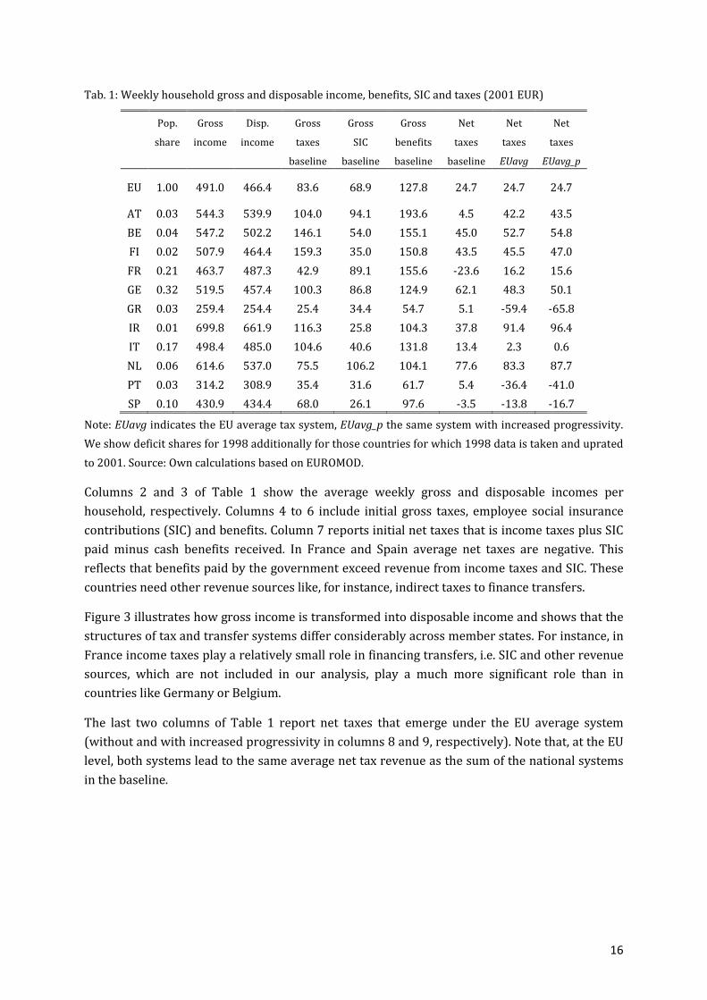
Tab. 1: Weekly household gross and disposable income, benefits, SIC and taxes (2001 EUR)

Pop.

share

Gross

income

Disp.

income

Gross

taxes

baseline

Gross

SIC

baseline

Gross

benefits

baseline

Net

taxes

baseline

Net

taxes

EUavg

Net

taxes

EUavg_p

EU 1.00 491.0 466.4 83.6 68.9 127.8 24.7 24.7 24.7

AT 0.03 544.3 539.9 104.0 94.1 193.6 4.5 42.2 43.5

BE 0.04 547.2 502.2 146.1 54.0 155.1 45.0 52.7 54.8

FI 0.02 507.9 464.4 159.3 35.0 150.8 43.5 45.5 47.0

FR 0.21 463.7 487.3 42.9 89.1 155.6 -23.6 16.2 15.6

GE 0.32 519.5 457.4 100.3 86.8 124.9 62.1 48.3 50.1

GR 0.03 259.4 254.4 25.4 34.4 54.7 5.1 -59.4 -65.8

IR 0.01 699.8 661.9 116.3 25.8 104.3 37.8 91.4 96.4

IT 0.17 498.4 485.0 104.6 40.6 131.8 13.4 2.3 0.6

NL 0.06 614.6 537.0 75.5 106.2 104.1 77.6 83.3 87.7

PT 0.03 314.2 308.9 35.4 31.6 61.7 5.4 -36.4 -41.0

SP 0.10 430.9 434.4 68.0 26.1 97.6 -3.5 -13.8 -16.7

Note: EUavg indicates the EU average tax system, EUavg_p the same system with increased progressivity.

We show deficit shares for 1998 additionally for those countries for which 1998 data is taken and uprated

to 2001. Source: Own calculations based on EUROMOD.

Columns 2 and 3 of Table 1 show the average weekly gross and disposable incomes per

household, respectively. Columns 4 to 6 include initial gross taxes, employee social insurance

contributions (SIC) and benefits. Column 7 reports initial net taxes that is income taxes plus SIC

paid minus cash benefits received. In France and Spain average net taxes are negative. This

reflects that benefits paid by the government exceed revenue from income taxes and SIC. These

countries need other revenue sources like, for instance, indirect taxes to finance transfers.

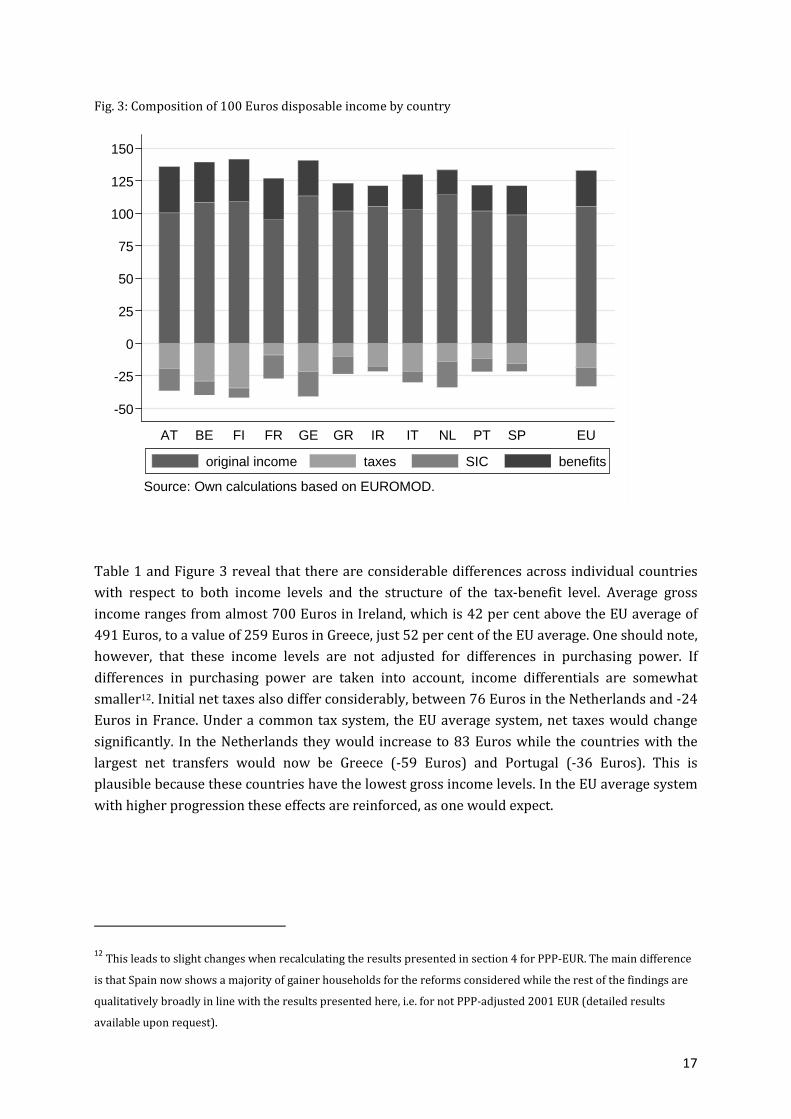
Figure 3 illustrates how gross income is transformed into disposable income and shows that the

structures of tax and transfer systems differ considerably across member states. For instance, in

France income taxes play a relatively small role in financing transfers, i.e. SIC and other revenue

sources, which are not included in our analysis, play a much more significant role than in

countries like Germany or Belgium.

The last two columns of Table 1 report net taxes that emerge under the EU average system

(without and with increased progressivity in columns 8 and 9, respectively). Note that, at the EU

level, both systems lead to the same average net tax revenue as the sum of the national systems

in the baseline.

17

Fig. 3: Composition of 100 Euros disposable income by country

Table 1 and Figure 3 reveal that there are considerable differences across individual countries

with respect to both income levels and the structure of the tax-benefit level. Average gross

income ranges from almost 700 Euros in Ireland, which is 42 per cent above the EU average of

491 Euros, to a value of 259 Euros in Greece, just 52 per cent of the EU average. One should note,

however, that these income levels are not adjusted for differences in purchasing power. If

differences in purchasing power are taken into account, income differentials are somewhat

smaller12. Initial net taxes also differ considerably, between 76 Euros in the Netherlands and -24

Euros in France. Under a common tax system, the EU average system, net taxes would change

significantly. In the Netherlands they would increase to 83 Euros while the countries with the

largest net transfers would now be Greece (-59 Euros) and Portugal (-36 Euros). This is

plausible because these countries have the lowest gross income levels. In the EU average system

with higher progression these effects are reinforced, as one would expect.

12 This leads to slight changes when recalculating the results presented in section 4 for PPP-EUR. The main difference

is that Spain now shows a majority of gainer households for the reforms considered while the rest of the findings are

qualitatively broadly in line with the results presented here, i.e. for not PPP-adjusted 2001 EUR (detailed results

available upon request).

-50

-25

0

25

50

75

100

125

150

AT BE FI FR GE GR IR IT NL PT SP EU


original income taxes SIC benefits

18

4 Results: Economic effects of a ‘fiscal union’

In this section we present and discuss the key results of our simulated policy scenarios. The

results are presented in five subsections. Section 4.1 focuses on the impact of introducing the

common EU tax system on the distribution of income. We consider the four scenarios described

in the previous section (share of the EU average system of 33.3% and 100%, respectively, with

and without increased progressivity). Throughout the analysis, behavioural effects in the form of

labour supply adjustments are accounted for. In the Appendix we summarise these effects

(Table C.2) and we also report results without behavioural adjustments (Table B.1).

In Section 4.2, we look at changes in inequality and a measure of social welfare which takes into

account inequality as a welfare reducing factor. For instance, a country with significant income

redistribution in its national system might not find a reform which increases average disposable

income of its households beneficial if this comes at the cost of an increase in inequality.

Subsequently, changes for income quintiles in the different countries are considered. In section

4.3, we are interested in whether a majority of voters benefits or loses because this may affect

political feasibility.

Section 4.4 investigates the potential of the EU average tax system to act as an automatic fiscal

stabiliser in presence of an asymmetric shock, compared to that of the current national tax-

benefit systems. While by construction, fiscal stabilisation is provided as a sum of national and

EU average stabilisation (in the scenarios where the EU system does not take over 100%), we

also look at the sole stabilisation effect of the EU average system. This is relevant in cases where

countries are credit constrained at the capital market, as is currently the case for some countries

in the Eurozone.

Finally, Section 4.5 turns to the issue of fiscal equalisation. There we propose a system of fiscal

equalisation which is based on differences in taxing capacity across countries. We calculate

transfers between countries that would be generated by this type of system and we consider a

scenario where a subset of countries – the GIIPS group – is affected by a negative

macroeconomic shock. We then calculate to which extent a fiscal equalisation mechanism would

provide insurance against this type of shock as well as against a shock comparable to the 2008-

09 recession.

4.1 Changes in disposable income and labour supply

We report the effects on disposable income accounting for labour supply effects which we

discuss first. We follow van Soest (1995) or Hoynes (1996) and estimate a structural discrete

choice labour supply model by specifying consumption-leisure preferences in a very flexible way

(and without imposing separability between consumption and leisure). The model is estimated

from the micro data and then used to predict the potential effects of a switch to the European

system. The labour supply model is described in detail in Appendix C, where also estimated

elasticities (Table C.1) as well as the labour supply effects (Table C.2 for the full population and

Tables C.3 and C.4 for subgroups) are reported.

The labour supply effects are negative in all winner countries except Germany and Finland. For

instance, in Greece and Spain overall labour supply falls, measured in full time equivalents, by

19

more than 2 per cent. However, in countries, where the most significant income losses occur,

labour supply effects are mostly positive, except for Ireland and Austria. Most substantial

reactions are observable for women in couples and single females, which corresponds to the

relatively high labour supply elasticities for this group as reported in Table C.1 in the Appendix.

For Austria, women in couples are the only group reducing their labour supply due to the

reform, which determines the direction of overall change in labour supply. For Germany, single

men are the only group reacting negatively to the introduction of the average system which

might reflect a substitution effect for those who initially worked full- or over-time and now

benefit from a reduced progressivity compared to the German tax-benefit system. For all other

countries the direction of overall labour supply effects and those for the subgroups is the same,

though, with substantial differences in magnitudes. Particularly large negative responses can be

observed for married and single women in Greece and Spain. For Greece, this will be partly due

to substitution effects initiated by the substantial increases in transfers while for Spain this

might reflect both, a substitution effect for those experiencing a shift in disposable income due to

more generous benefits and an income effect for higher income earners suffering from increased

progressivity (see also again Figure 2).

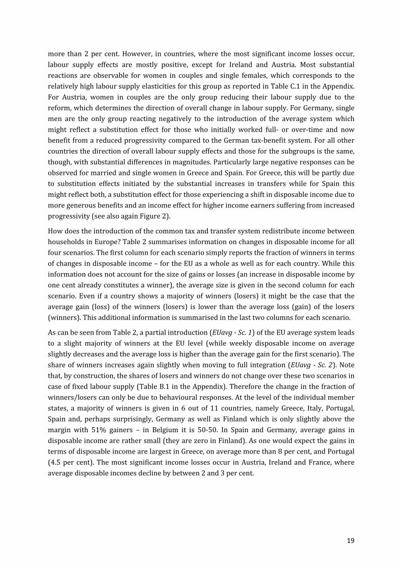
How does the introduction of the common tax and transfer system redistribute income between

households in Europe? Table 2 summarises information on changes in disposable income for all

four scenarios. The first column for each scenario simply reports the fraction of winners in terms

of changes in disposable income – for the EU as a whole as well as for each country. While this

information does not account for the size of gains or losses (an increase in disposable income by

one cent already constitutes a winner), the average size is given in the second column for each

scenario. Even if a country shows a majority of winners (losers) it might be the case that the

average gain (loss) of the winners (losers) is lower than the average loss (gain) of the losers

(winners). This additional information is summarised in the last two columns for each scenario.

As can be seen from Table 2, a partial introduction (EUavg - Sc. 1) of the EU average system leads

to a slight majority of winners at the EU level (while weekly disposable income on average

slightly decreases and the average loss is higher than the average gain for the first scenario). The

share of winners increases again slightly when moving to full integration (EUavg - Sc. 2). Note

that, by construction, the shares of losers and winners do not change over these two scenarios in

case of fixed labour supply (Table B.1 in the Appendix). Therefore the change in the fraction of

winners/losers can only be due to behavioural responses. At the level of the individual member

states, a majority of winners is given in 6 out of 11 countries, namely Greece, Italy, Portugal,

Spain and, perhaps surprisingly, Germany as well as Finland which is only slightly above the

margin with 51% gainers – in Belgium it is 50-50. In Spain and Germany, average gains in

disposable income are rather small (they are zero in Finland). As one would expect the gains in

terms of disposable income are largest in Greece, on average more than 8 per cent, and Portugal

(4.5 per cent). The most significant income losses occur in Austria, Ireland and France, where

average disposable incomes decline by between 2 and 3 per cent.

20

Tab. 2: % gainers, overall %-change, mean gain and loss in weekly disposable income (2001 EUR)

EUavg – Sc. 1 EUavg – Sc. 2 EUavg_p – Sc. 1 EUavg_p – Sc. 2

%+ %dY Gap+ Gap- %+ %dY Gap+ Gap- %+ %dY Gap+ Gap- %+ %dY Gap+ Gap-

EU 55 0.0 19.9 -23.6 56 0.5 60.0 -70.5 53 0.0 21.1 -23.8 54 0.4 63.8 -70.8

AT 35 -2.2 17.2 -28.3 36 -6.5 51.1 -85.0 32 -2.4 18.7 -27.7 33 -6.8 54.7 -83.0

BE 50 -0.3 19.2 -22.3 51 -0.5 58.0 -66.6 44 -0.5 19.1 -19.8 46 -1.2 56.6 -59.1

FI 51 0.0 19.1 -19.6 53 0.7 57.1 -58.6 49 -0.1 18.4 -19.3 51 0.1 54.9 -57.4

FR 31 -2.8 14.5 -26.5 32 -7.9 42.5 -78.6 30 -2.8 17.3 -26.9 31 -7.9 51.0 -79.6

GE 66 1.0 20.0 -24.5 68 3.6 60.7 -74.0 64 0.8 19.3 -23.2 66 3.0 58.7 -69.6

GR 80 8.5 30.8 -12.7 80 26.1 93.6 -38.2 79 9.3 34.0 -13.4 80 28.8 103.4 -40.5

IR 28 -2.7 21.2 -33.8 29 -7.6 63.3 -98.4 28 -3.0 25.6 -38.0 29 -8.2 76.5 -109.9

IT 63 0.9 19.6 -21.8 63 2.8 59.7 -65.8 62 1.0 21.7 -22.1 62 3.3 66.1 -66.6

NL 40 -0.6 16.8 -16.5 41 -1.3 50.1 -47.4 38 -0.9 19.9 -20.6 39 -2.2 59.0 -58.9

PT 68 4.5 29.4 -17.9 69 13.6 87.8 -54.0 67 5.0 33.0 -18.6 67 15.0 99.2 -55.7

SP 60 0.9 20.1 -20.2 61 3.1 61.0 -60.8 59 1.1 23.2 -21.3 61 4.0 70.1 -63.5

Note: %+ is the percentage of reform gainers (100 minus %+ is the percentage of reform losers);

%dY the overall %-change in household weekly mean disposable income; Gap+ (Gap-) the mean

difference from zero for positive (negative) dY. Source: Own calculations based on EUROMOD.

An interesting aspect of this result is that intuitively, one would assume that the rich countries

systematically lose in a common system. This is only partly true. It is particularly puzzling that

Germany and France are affected very differently, with France losing significantly although its

average income is lower. The explanation for this finding is that the national tax and transfer

systems of these two countries are very different, despite their similarity in other dimensions.

Inspecting Figure 2 shows that, indeed, the EU tax system implies higher taxes and lower

transfers than the French national system. This implies that the net tax burden on the French

population increases. In addition, French income levels are close to the EU average, so that the

country cannot hope to benefit from participating in a system with higher average incomes.

Figure 5 shows that in France the low income quintiles suffer more than the high income

quintiles. In Germany, however, the situation is different. The national tax and transfer system is

characterised by higher progressivity and slightly higher taxes for high income earners. For

lower income levels, the distance between the national and the EU tax and transfer system is

rather small. As a result, all quintiles in Germany gain from the introduction of the EU tax.

The general pattern of results in terms of losers and winners at the country level (as well as in

terms of the direction in labour supply responses) is robust when switching to the EU average

tax system with an increase in tax progressivity (EUavg_p - Sc. 1, Sc. 2). The numbers of winners

and losers change slightly, as do the magnitudes of average gains and losses. But – except for the

case of partial integration where Finland now has slightly less gainers (49%) than losers - no

country shows a shift from a majority of losers to a majority of winners or vice versa.

21

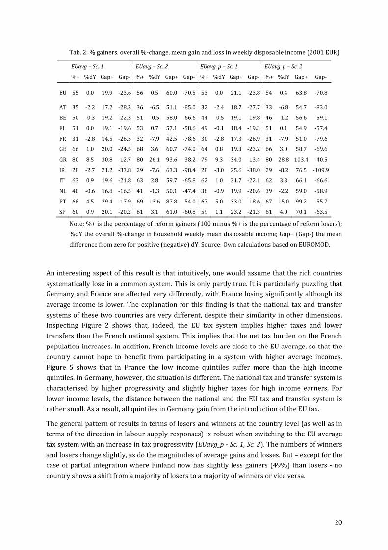
4.2 Effects on welfare and inequality

Changes in inequality due to the redistributive effects of tax-benefit reforms will also be a

relevant indicator to policy makers. Therefore, Table 3 additionally reports the Gini coefficient

across countries as well as its percentage change due to the introduction of the different

scenarios. Next, this information is integrated with the change in disposable income into a social

welfare function (SWF) of the Yitzhaki-type (Yitzhaki, 1979), i.e. Y = Z ∗ (1 − �) withZ the

mean disposable income of the respective population and G the accordant Gini index.13

Table 3 reveals that, at least in the first two scenarios, the pattern of winner and loser countries

does not change when looking at welfare instead of disposable income, i.e. it is again the same

group of countries - Germany, Greece, Italy, Portugal and Spain (but not Finland) - that benefits

in terms of the percentage change in social welfare. Inequality also declines in the EU as a whole,

as well as in all individual countries except Belgium and Finland. Greece is again the country that

benefits most, showing the largest decrease in the Gini coefficient (having the highest level of

initial inequality). When moving to the average system with increased progressivity, the overall

pattern again does not change (minor changes can be observed for Finland and the

Netherlands). However, as can be expected, decreases (increases) in inequality (increases

(decreases) in welfare) become stronger (less strong or even negative) compared to the

scenarios without increased progressivity.

Tab. 3: Gini-Index (G, %-changes dG) and Welfare (W, %-changes dW)

Baseline EUavg – Sc. 1 EUavg – Sc. 2 EUavg_p – Sc. 1 EUavg_p – Sc. 2

G W dG dW dG dW dG dW dG dW

EU 0.34 315 -3.2 1.7 -6.4 3.8 -4.5 2.4 -10.5 6.0

AT 0.31 382 -0.4 -2.1 3.5 -7.9 -1.8 -1.6 -1.2 -6.3

BE 0.33 347 1.8 -1.2 8.1 -4.4 0.1 -0.6 2.9 -2.6

FI 0.34 315 1.0 -0.5 5.1 -2.0 -0.4 0.1 1.2 -0.6

FR 0.31 343 -2.1 -1.9 -2.4 -6.9 -3.5 -1.2 -6.9 -5.0

GE 0.33 323 -2.8 2.4 -5.5 6.3 -4.4 3.0 -10.3 8.2

GR 0.42 151 -12.8 18.4 -27.4 50.7 -14.3 20.5 -29.8 56.2

IR 0.36 432 -1.3 -2.0 -3.1 -6.0 -2.4 -1.7 -6.2 -5.1

IT 0.37 307 -4.0 3.2 -9.5 8.6 -5.2 4.1 -13.0 11.2

NL 0.31 391 -1.1 -0.1 -2.2 -0.3 -2.4 0.2 -5.9 0.3

PT 0.40 191 -8.0 10.1 -16.3 25.9 -9.4 11.5 -18.7 29.3

SP 0.37 281 -4.5 3.5 -10.9 9.6 -5.7 4.4 -14.1 12.5


13 In Appendix D, we show that the results do no change when aggregating the individual utilities from the labor

supply model using a utilitarian SWF.

22

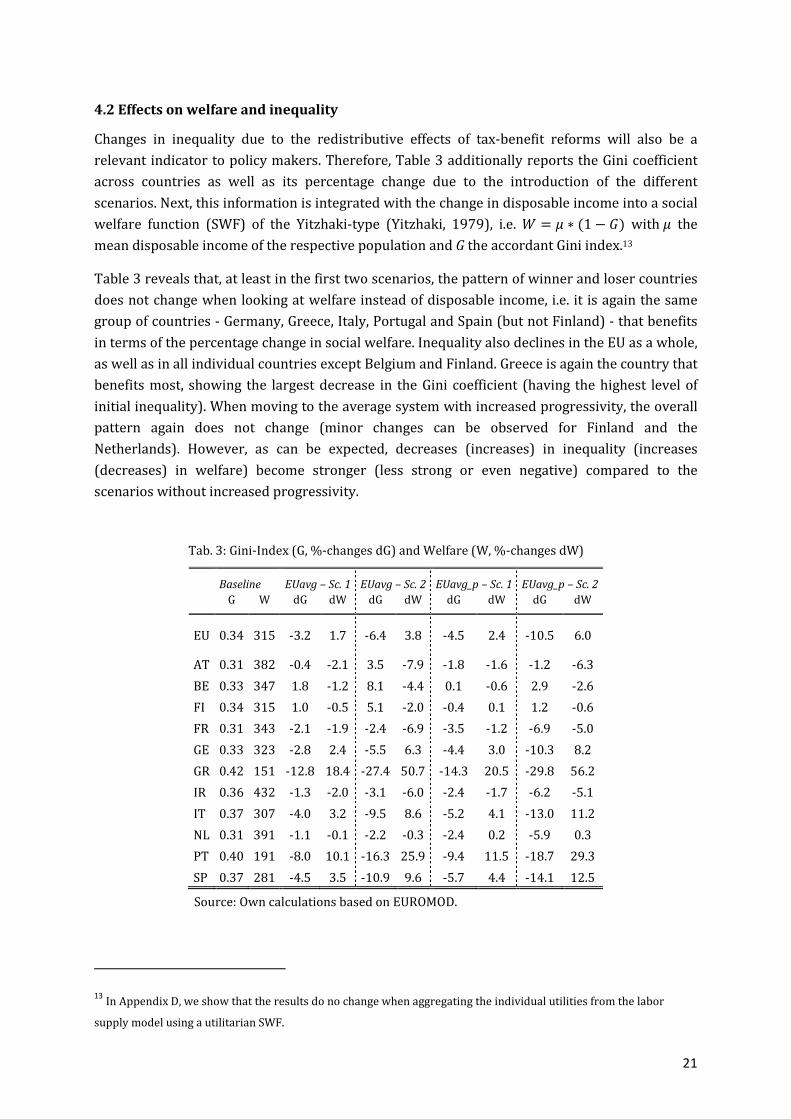
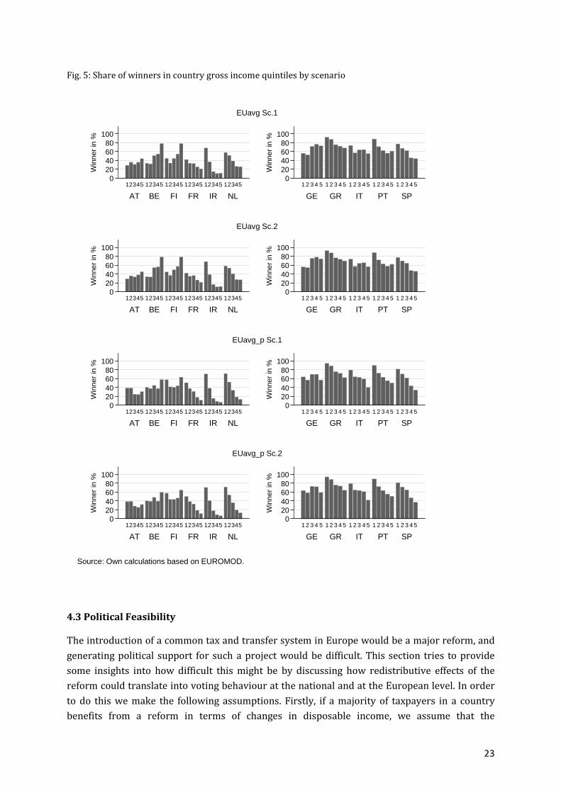
Related to that, Figure 4 shows the share of winners within gross income quintiles of the overall

sample population by scenario. The effects are rather similar for all quintiles of the overall EU

income distribution. The effect of increased progressivity becomes visible as well: the share of

winners increases with higher progressivity for quintiles 1 and 2 while for the fourth and the

fifth quintile, it is the share of losers that increases.

Fig. 4: Share of winners in global quintiles by reform scenario

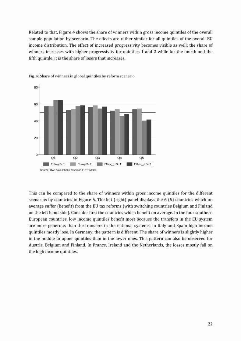
This can be compared to the share of winners within gross income quintiles for the different

scenarios by countries in Figure 5. The left (right) panel displays the 6 (5) countries which on

average suffer (benefit) from the EU tax reforms (with switching countries Belgium and Finland

on the left hand side). Consider first the countries which benefit on average. In the four southern

European countries, low income quintiles benefit most because the transfers in the EU system

are more generous than the transfers in the national systems. In Italy and Spain high income

quintiles mostly lose. In Germany, the pattern is different. The share of winners is slightly higher

in the middle to upper quintiles than in the lower ones. This pattern can also be observed for

Austria, Belgium and Finland. In France, Ireland and the Netherlands, the losses mostly fall on

the high income quintiles.

0

20

40

60

80

Q1 Q2 Q3 Q4 Q5


EUavg Sc.1 EUavg Sc.2 EUavg_p Sc.1 EUavg_p Sc.2

23

Fig. 5: Share of winners in country gross income quintiles by scenario

4.3 Political Feasibility

The introduction of a common tax and transfer system in Europe would be a major reform, and

generating political support for such a project would be difficult. This section tries to provide

some insights into how difficult this might be by discussing how redistributive effects of the

reform could translate into voting behaviour at the national and at the European level. In order

to do this we make the following assumptions. Firstly, if a majority of taxpayers in a country

benefits from a reform in terms of changes in disposable income, we assume that the

020406080

100

Win

ner

in %

AT BE FI FR IR NL

12345 12345 12345 12345 12345 123450

20406080

100

Win

ner

in %

GE GR IT PT SP

1 2 3 4 5 1 2 3 4 5 1 2 3 4 5 1 2 3 4 5 1 2 3 4 5

EUavg Sc.1

020406080

100

Win

ner

in %

AT BE FI FR IR NL

12345 12345 12345 12345 12345 123450

20406080

100

Win

ner

in %

GE GR IT PT SP

1 2 3 4 5 1 2 3 4 5 1 2 3 4 5 1 2 3 4 5 1 2 3 4 5

EUavg Sc.2

020406080

100

Win

ner

in %

AT BE FI FR IR NL

12345 12345 12345 12345 12345 123450

20406080

100

Win

ner

in %

GE GR IT PT SP

1 2 3 4 5 1 2 3 4 5 1 2 3 4 5 1 2 3 4 5 1 2 3 4 5

EUavg_p Sc.1

020406080

100

Win

ner

in %

AT BE FI FR IR NL

12345 12345 12345 12345 12345 123450

20406080

100

Win

ner

in %

GE GR IT PT SP

1 2 3 4 5 1 2 3 4 5 1 2 3 4 5 1 2 3 4 5 1 2 3 4 5

EUavg_p Sc.2


24

government of this country will support the reform when it comes to voting at the European

level, independently of the extent of gains and losses.

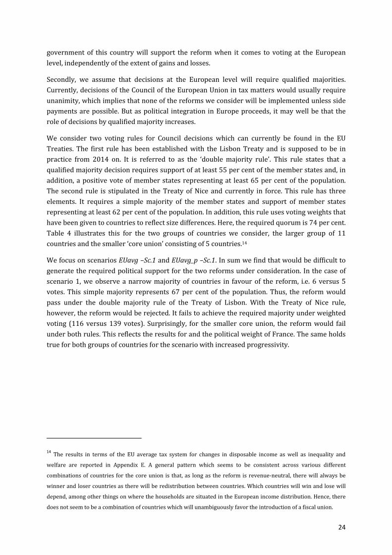
Secondly, we assume that decisions at the European level will require qualified majorities.

Currently, decisions of the Council of the European Union in tax matters would usually require

unanimity, which implies that none of the reforms we consider will be implemented unless side

payments are possible. But as political integration in Europe proceeds, it may well be that the

role of decisions by qualified majority increases.

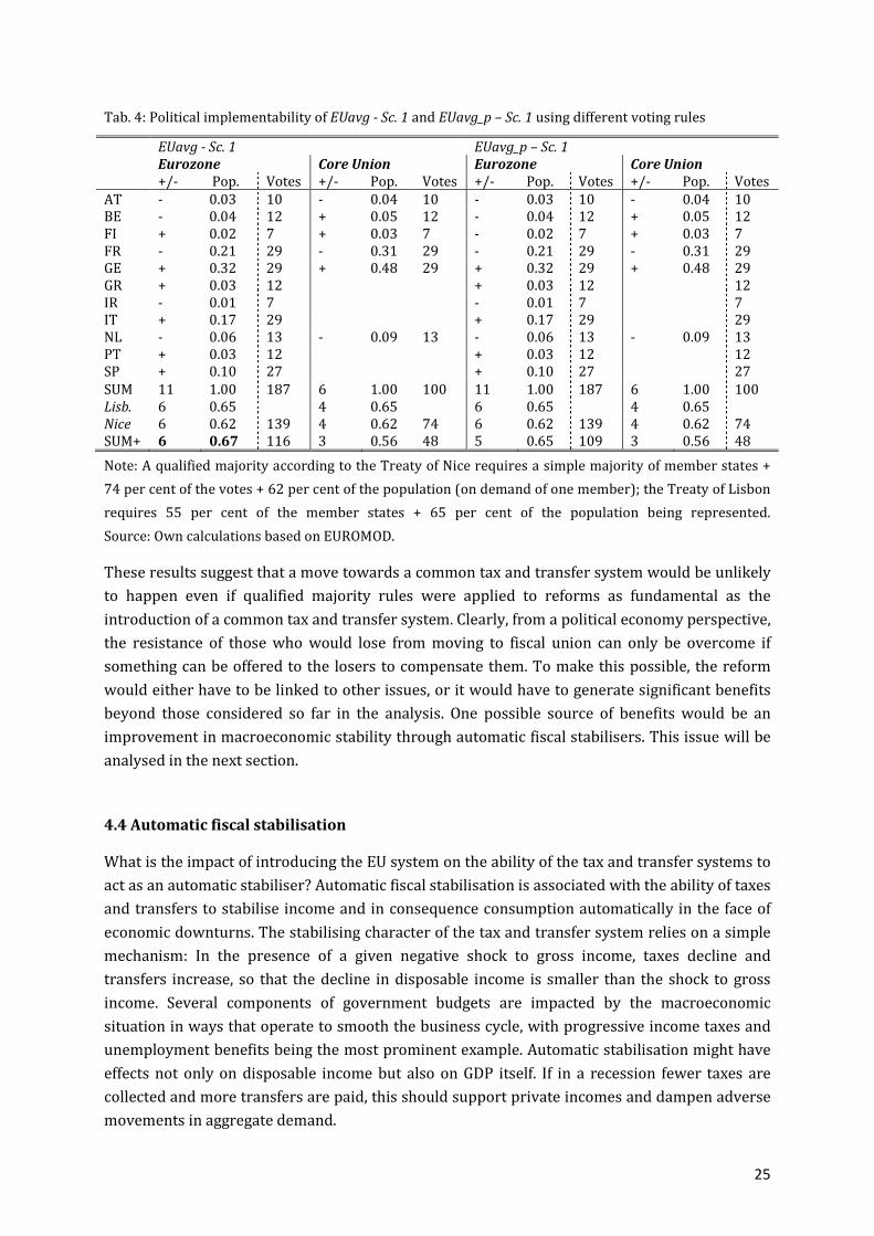
We consider two voting rules for Council decisions which can currently be found in the EU

Treaties. The first rule has been established with the Lisbon Treaty and is supposed to be in

practice from 2014 on. It is referred to as the ‘double majority rule’. This rule states that a

qualified majority decision requires support of at least 55 per cent of the member states and, in

addition, a positive vote of member states representing at least 65 per cent of the population.

The second rule is stipulated in the Treaty of Nice and currently in force. This rule has three

elements. It requires a simple majority of the member states and support of member states

representing at least 62 per cent of the population. In addition, this rule uses voting weights that

have been given to countries to reflect size differences. Here, the required quorum is 74 per cent.

Table 4 illustrates this for the two groups of countries we consider, the larger group of 11

countries and the smaller ‘core union’ consisting of 5 countries.14

We focus on scenarios EUavg –Sc.1 and EUavg_p –Sc.1. In sum we find that would be difficult to

generate the required political support for the two reforms under consideration. In the case of

scenario 1, we observe a narrow majority of countries in favour of the reform, i.e. 6 versus 5

votes. This simple majority represents 67 per cent of the population. Thus, the reform would

pass under the double majority rule of the Treaty of Lisbon. With the Treaty of Nice rule,

however, the reform would be rejected. It fails to achieve the required majority under weighted

voting (116 versus 139 votes). Surprisingly, for the smaller core union, the reform would fail

under both rules. This reflects the results for and the political weight of France. The same holds

true for both groups of countries for the scenario with increased progressivity.

14 The results in terms of the EU average tax system for changes in disposable income as well as inequality and

welfare are reported in Appendix E. A general pattern which seems to be consistent across various different

combinations of countries for the core union is that, as long as the reform is revenue-neutral, there will always be

winner and loser countries as there will be redistribution between countries. Which countries will win and lose will

depend, among other things on where the households are situated in the European income distribution. Hence, there

does not seem to be a combination of countries which will unambiguously favor the introduction of a fiscal union.

25

Tab. 4: Political implementability of EUavg - Sc. 1 and EUavg_p – Sc. 1 using different voting rules

EUavg - Sc. 1 EUavg_p – Sc. 1

Eurozone Core Union Eurozone Core Union

+/- Pop. Votes +/- Pop. Votes +/- Pop. Votes +/- Pop. Votes AT - 0.03 10 - 0.04 10 - 0.03 10 - 0.04 10 BE - 0.04 12 + 0.05 12 - 0.04 12 + 0.05 12 FI + 0.02 7 + 0.03 7 - 0.02 7 + 0.03 7 FR - 0.21 29 - 0.31 29 - 0.21 29 - 0.31 29 GE + 0.32 29 + 0.48 29 + 0.32 29 + 0.48 29 GR + 0.03 12 + 0.03 12 12 IR - 0.01 7 - 0.01 7 7 IT + 0.17 29 + 0.17 29 29 NL - 0.06 13 - 0.09 13 - 0.06 13 - 0.09 13 PT + 0.03 12 + 0.03 12 12 SP + 0.10 27 + 0.10 27 27 SUM 11 1.00 187 6 1.00 100 11 1.00 187 6 1.00 100 Lisb. 6 0.65 4 0.65 6 0.65 4 0.65 Nice 6 0.62 139 4 0.62 74 6 0.62 139 4 0.62 74 SUM+ 6 0.67 116 3 0.56 48 5 0.65 109 3 0.56 48

Note: A qualified majority according to the Treaty of Nice requires a simple majority of member states +

74 per cent of the votes + 62 per cent of the population (on demand of one member); the Treaty of Lisbon

requires 55 per cent of the member states + 65 per cent of the population being represented.


These results suggest that a move towards a common tax and transfer system would be unlikely

to happen even if qualified majority rules were applied to reforms as fundamental as the

introduction of a common tax and transfer system. Clearly, from a political economy perspective,

the resistance of those who would lose from moving to fiscal union can only be overcome if

something can be offered to the losers to compensate them. To make this possible, the reform

would either have to be linked to other issues, or it would have to generate significant benefits

beyond those considered so far in the analysis. One possible source of benefits would be an

improvement in macroeconomic stability through automatic fiscal stabilisers. This issue will be

analysed in the next section.

4.4 Automatic fiscal stabilisation

What is the impact of introducing the EU system on the ability of the tax and transfer systems to

act as an automatic stabiliser? Automatic fiscal stabilisation is associated with the ability of taxes

and transfers to stabilise income and in consequence consumption automatically in the face of

economic downturns. The stabilising character of the tax and transfer system relies on a simple

mechanism: In the presence of a given negative shock to gross income, taxes decline and

transfers increase, so that the decline in disposable income is smaller than the shock to gross

income. Several components of government budgets are impacted by the macroeconomic

situation in ways that operate to smooth the business cycle, with progressive income taxes and

unemployment benefits being the most prominent example. Automatic stabilisation might have

effects not only on disposable income but also on GDP itself. If in a recession fewer taxes are

collected and more transfers are paid, this should support private incomes and dampen adverse

movements in aggregate demand.

26

Of course, cushioning of shocks through taxes and transfers comes at the cost of an increase in

the government budget deficit. The usual assumption is that this gap is closed through debt

financing. However, in the current Eurozone debt crisis, some countries have lost access to

private capital markets so that they need outside help to close the gap in the government budget.

We will return to this issue further below.

The extent to which automatic stabilisers mitigate the impact of income shocks on household

demand essentially depends on the tax and transfer system which determines the way in which

a given shock to gross income translates into a change in disposable income. For instance, in the

presence of a proportional income tax with a tax rate of 40%, a shock on gross income of 100

Euros leads to a decline in disposable income of 60 Euros. In this case, the tax absorbs 40% of

the shock to gross income. A progressive tax, in turn, would have a stronger stabilising effect

(van den Noord, 2000; Girouard and André, 2005).

A common measure for estimating automatic stabilisation is the “normalised tax change” used

by Auerbach and Feenberg (2000) which can be interpreted as “the tax system’s built-in

flexibility” (Pechman, 1973, 1987). Based on this idea, in Dolls et al. (2012) define the “income

stabilization coefficient” [ which shows how changes in market income (defined as the sum of all

incomes from market activities such as (self)-employment, business and property income)

\translate into changes in disposable income (market income minus taxes plus benefits)

]through changes in net tax payments G. They extend the concept of normalised tax change to

include other taxes as well as social insurance contributions and transfers like e.g.

unemployment benefits. We follow their approach and take into account personal income taxes

(at all government levels), social insurance contributions as well as payroll taxes and transfers

to private households such as unemployment benefits. τ is computed using arithmetic changes

(Δ) in total disposable income (∑ ∆�]� ) and market income (∑ ∆�\� ) based on household micro

level information:

[ = 1 − ∑ ∆_�`�∑ ∆_�a�

= ∑ (∆_�a ∆_�`)�∑ ∆_�a�

. (12)

In order to compute the coefficients of automatic stabilisation, we compute their income shock

measure defined as a proportional decrease of gross income by 5% for all households. The

results are presented in Table 5. The levels and differences across countries in the baseline

scenario are in line with the calculations in Dolls et al. (2012).

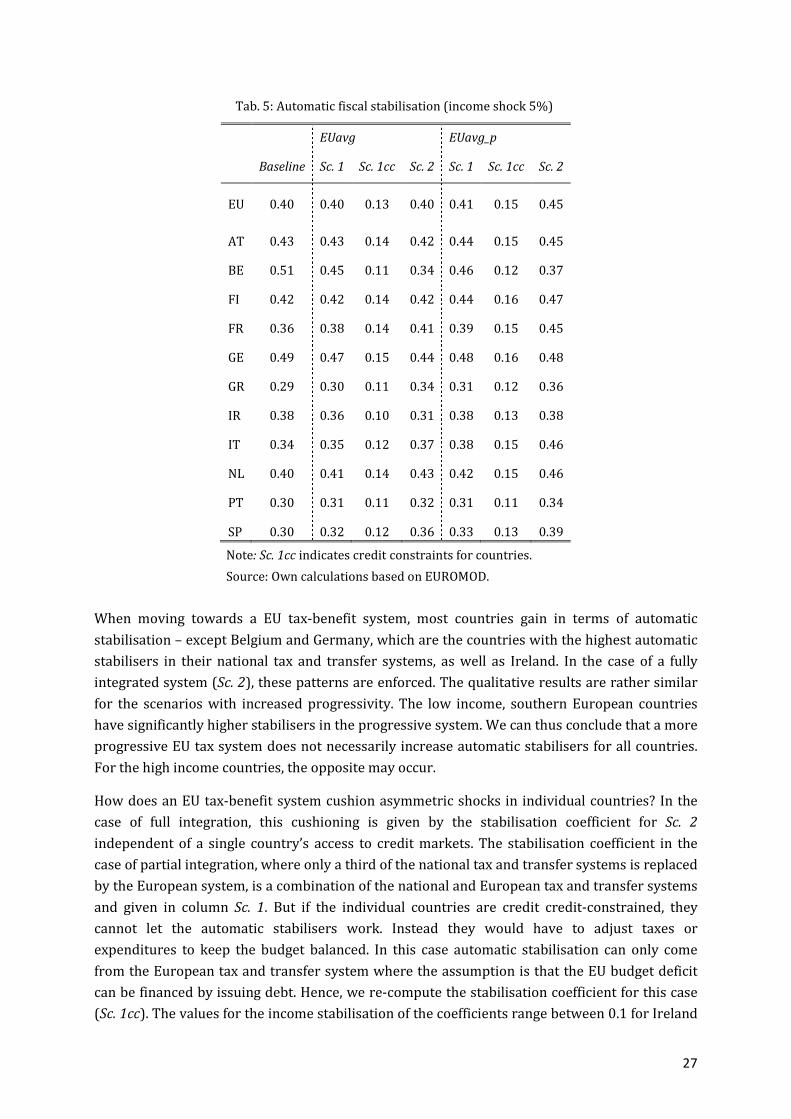
27

Tab. 5: Automatic fiscal stabilisation (income shock 5%)

EUavg EUavg_p

Baseline Sc. 1 Sc. 1cc Sc. 2 Sc. 1 Sc. 1cc Sc. 2

EU 0.40 0.40 0.13 0.40 0.41 0.15 0.45

AT 0.43 0.43 0.14 0.42 0.44 0.15 0.45

BE 0.51 0.45 0.11 0.34 0.46 0.12 0.37

FI 0.42 0.42 0.14 0.42 0.44 0.16 0.47

FR 0.36 0.38 0.14 0.41 0.39 0.15 0.45

GE 0.49 0.47 0.15 0.44 0.48 0.16 0.48

GR 0.29 0.30 0.11 0.34 0.31 0.12 0.36

IR 0.38 0.36 0.10 0.31 0.38 0.13 0.38

IT 0.34 0.35 0.12 0.37 0.38 0.15 0.46

NL 0.40 0.41 0.14 0.43 0.42 0.15 0.46

PT 0.30 0.31 0.11 0.32 0.31 0.11 0.34

SP 0.30 0.32 0.12 0.36 0.33 0.13 0.39

Note: Sc. 1cc indicates credit constraints for countries.


When moving towards a EU tax-benefit system, most countries gain in terms of automatic

stabilisation – except Belgium and Germany, which are the countries with the highest automatic

stabilisers in their national tax and transfer systems, as well as Ireland. In the case of a fully

integrated system (Sc. 2), these patterns are enforced. The qualitative results are rather similar

for the scenarios with increased progressivity. The low income, southern European countries

have significantly higher stabilisers in the progressive system. We can thus conclude that a more

progressive EU tax system does not necessarily increase automatic stabilisers for all countries.

For the high income countries, the opposite may occur.

How does an EU tax-benefit system cushion asymmetric shocks in individual countries? In the

case of full integration, this cushioning is given by the stabilisation coefficient for Sc. 2

independent of a single country’s access to credit markets. The stabilisation coefficient in the

case of partial integration, where only a third of the national tax and transfer systems is replaced

by the European system, is a combination of the national and European tax and transfer systems

and given in column Sc. 1. But if the individual countries are credit credit-constrained, they

cannot let the automatic stabilisers work. Instead they would have to adjust taxes or

expenditures to keep the budget balanced. In this case automatic stabilisation can only come

from the European tax and transfer system where the assumption is that the EU budget deficit

can be financed by issuing debt. Hence, we re-compute the stabilisation coefficient for this case

(Sc. 1cc). The values for the income stabilisation of the coefficients range between 0.1 for Ireland

28

and 0.15 for Germany and are at approximately one third (i.e. its share) of the EU average

system. In the case of the more progressive EU system, the automatic stabilisers slightly increase

for all countries. On average, the automatic stabilisers of the EU budget would absorb

approximately 15 per cent of an income shock. This illustrates that even a rather radical reform,

which replaces one third of the national tax and transfer systems by a supranational system,

would have only rather moderate fiscal stabilisation effects in the event of country specific

shocks.

4.5. Fiscal Equalisation

We now turn to the second element of a fiscal union in our analysis, the introduction of a fiscal

equalisation mechanism. Fiscal equalisation, in contrast to the creation of a common tax and

transfer system, leaves the national tax and transfer systems in place but redistributes tax

revenue across countries. This redistribution is based on the hypothetical ability of a country to

generate tax revenue, to which we refer as its taxing capacity. In existing fiscal equalisation

systems this is a common approach (see e.g. Boadway, 2004, or Büttner, 2006). We define the

taxing capacity of a country as the net tax revenue a country would raise if it fully applied the ‘EU

average’ tax and transfer system used in the preceding section (compare Table 1, column ‘Net

taxes EUavg’). This taxing capacity can be interpreted as an indicator of the amount of tax

revenue that could be raised by a country if tax rates and transfers were set as in other countries

and serves as the basis for equalisation payments. Countries above (below) the average taxable

capacity will pay (receive) transfers to (from) the equalisation mechanism. This setup can be

interpreted as a simple version of a European ‘transfer union’. Note that the scenario considered

here is quite ambitious in that the fiscal equalisation scenario fully compensates for differences

in taxing capacity. In practice one might expect a more moderate system which would

compensate countries for a share of the differences in taxing capacity only.

It is clear that in such a system, a country as a whole either gains or loses, depending on whether

the country is a net donor or recipient of fiscal equalisation payments. The distribution of taxes

and transfers within a country, however, is less straightforward. For simplicity, and in order not

to alter existing redistribution within a country, we assume that the equalisation of taxes and

transfers are shared among households proportionally to existing net tax payments. What are

the implications for automatic stabilisation properties of the tax and transfer system? Table 6

shows the net tax payments in the baseline as well as for the EU average system which serves as

our measure of taxable capacity. The resulting fiscal equalisation payments are reported in

column 3 (a positive (negative) value indicates a net contributing (receiving) country). Column 4

includes the new distribution of net taxes.

Consider first the direct cross country distributional effect of the fiscal equalisation system. As

one would expect, the high income countries are net contributors to the system. Contributions

per household range from 66.7 Euros in the case of Ireland to 17.5 Euros in Austria. These are

huge contributions, equivalent to 9.6 per cent of gross income in Ireland and 3.2 per cent of

gross income in Austria. Clearly, these unrealistically large contributions reflect the fact that the

degree of fiscal equalisation is 100 per cent. Accordingly, the countries with below average

taxing capacity receive huge transfers. The recipients include Greece, Portugal, Spain, Italy and

France. In Greece the fiscal equalisation payment is equal to 84 Euros, an implausible 33 per cent

29

of average gross income. France receives the lowest payment per household, just 8.5 Euros,

which equals 1.7 per cent of average gross income.

What are the implications of this system for automatic stabilisers? As long as governments can

cushion income shocks by increasing debt financing, the stabilisers in the system are the same as

under the national systems. But things are different if governments cannot borrow without

restrictions. Consider an asymmetric shock in the form of a decline in gross incomes by 5%

which hits the periphery of the Eurozone, i.e. the GIIPS countries. This corresponds to a 2%

shock at the EU level (column 5). The shock leads to a reduction in the net tax payments

collected in the affected countries (column 6) as well as a reduction in their taxable capacity

(column 7). As a result, the fiscal equalisation payments for all countries have to be adjusted

(column 8) resulting in a new distribution of net taxes (column 9). Finally, column 10 reports the

automatic stabilisation effect of the fiscal equalisation scheme in the affected countries. It

measures the change in fiscal equalisation payments as a percentage of the change in income

caused by the shock. Negative values of dAS imply that payments received from the fiscal

equalisation scheme decline in response to the negative shock or contributions a country has to

make to the scheme increase, so that a destabilising effect arises.

Tab 6: 5% asymmetric shock to GIIPS countries with fiscal equalisation mechanism

Net Net Fiscal Fiscal Gross New net New net New New dAS

taxes taxes eq. eq. income taxes taxes fiscal. fiscal fiscal

baseline EUavg taxes shock % nat. EUavg eq. eq. taxes eq.

EU 24.5 24.5 0.0 24.5 2 22.0 22.0 0.0 22.0 7

AT 4.5 42.2 17.5 22.0 0 4.5 42.2 20.1 24.6 0

BE 45.0 52.7 28.0 73.0 0 45.0 52.7 30.6 75.6 0

FI 43.5 45.5 20.8 64.3 0 43.5 45.5 23.4 66.9 0

FR -23.6 16.2 -8.5 -32.1 0 -23.6 16.2 -5.9 -29.5 0

GE 62.1 48.3 23.6 85.7 0 62.1 48.3 26.2 88.3 0

GR 5.1 -59.4 -84.1 -79.1 5 1.1 -61.9 -84.0 -82.9 -1

IR 37.8 91.4 66.7 104.5 5 23.3 77.4 55.3 78.6 33

IT 13.4 2.3 -22.4 -9.0 5 4.5 -7.0 -29.1 -24.6 27

NL 77.6 83.3 58.6 136.2 0 77.6 83.3 61.2 138.8 0

PT 5.4 -36.4 -61.1 -55.7 5 0.5 -40.2 -62.3 -61.8 8

SP -3.5 -13.8 -38.5 -42.0 5 -9.8 -21.1 -43.2 -53.1 22

Note: Monetary values are in weekly 2001 EUR. Source: Own calculations based on EUROMOD.

Maybe the most striking result is that the fiscal equalisation system may have a destabilising,

rather than a stabilising impact on some of the countries hit by the shock. In our scenario this

applies to Greece, the country most favoured by the initial fiscal equalisation system. Although

its fiscal capacity declines as a consequence of the shock, the payment it receives from the fiscal

equalisation system declines slightly. The payment received by Portugal is almost unchanged.

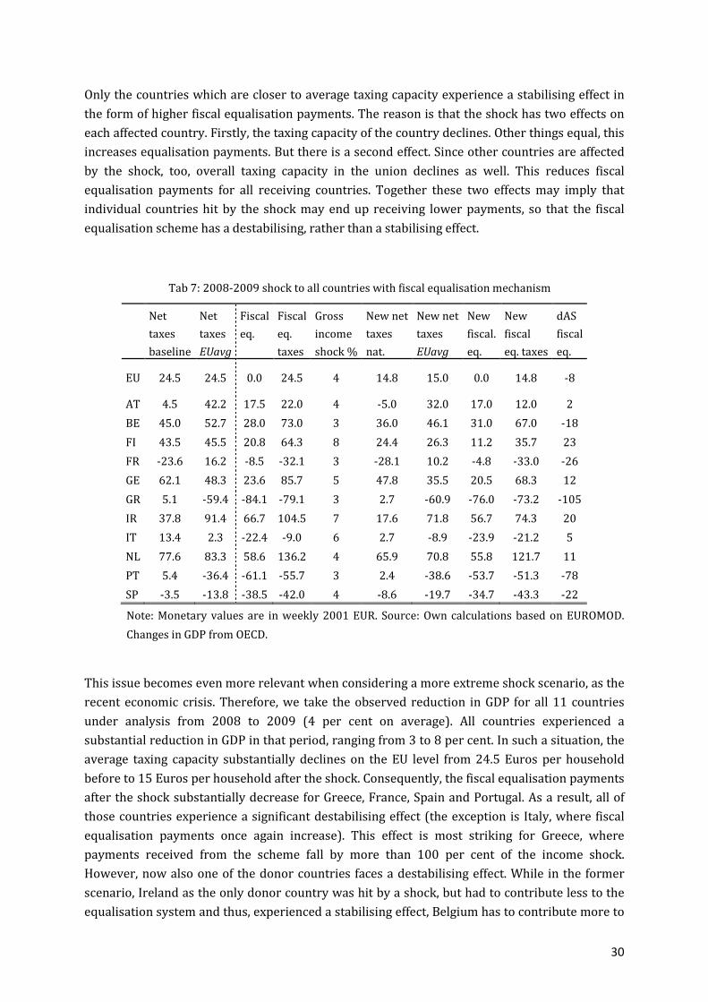
30

Only the countries which are closer to average taxing capacity experience a stabilising effect in

the form of higher fiscal equalisation payments. The reason is that the shock has two effects on

each affected country. Firstly, the taxing capacity of the country declines. Other things equal, this

increases equalisation payments. But there is a second effect. Since other countries are affected

by the shock, too, overall taxing capacity in the union declines as well. This reduces fiscal

equalisation payments for all receiving countries. Together these two effects may imply that

individual countries hit by the shock may end up receiving lower payments, so that the fiscal

equalisation scheme has a destabilising, rather than a stabilising effect.

Tab 7: 2008-2009 shock to all countries with fiscal equalisation mechanism

Net Net Fiscal Fiscal Gross New net New net New New dAS

taxes taxes eq. eq. income taxes taxes fiscal. fiscal fiscal

baseline EUavg taxes shock % nat. EUavg eq. eq. taxes eq.

EU 24.5 24.5 0.0 24.5 4 14.8 15.0 0.0 14.8 -8

AT 4.5 42.2 17.5 22.0 4 -5.0 32.0 17.0 12.0 2

BE 45.0 52.7 28.0 73.0 3 36.0 46.1 31.0 67.0 -18

FI 43.5 45.5 20.8 64.3 8 24.4 26.3 11.2 35.7 23

FR -23.6 16.2 -8.5 -32.1 3 -28.1 10.2 -4.8 -33.0 -26

GE 62.1 48.3 23.6 85.7 5 47.8 35.5 20.5 68.3 12

GR 5.1 -59.4 -84.1 -79.1 3 2.7 -60.9 -76.0 -73.2 -105

IR 37.8 91.4 66.7 104.5 7 17.6 71.8 56.7 74.3 20

IT 13.4 2.3 -22.4 -9.0 6 2.7 -8.9 -23.9 -21.2 5

NL 77.6 83.3 58.6 136.2 4 65.9 70.8 55.8 121.7 11

PT 5.4 -36.4 -61.1 -55.7 3 2.4 -38.6 -53.7 -51.3 -78

SP -3.5 -13.8 -38.5 -42.0 4 -8.6 -19.7 -34.7 -43.3 -22

Note: Monetary values are in weekly 2001 EUR. Source: Own calculations based on EUROMOD.

Changes in GDP from OECD.

This issue becomes even more relevant when considering a more extreme shock scenario, as the

recent economic crisis. Therefore, we take the observed reduction in GDP for all 11 countries

under analysis from 2008 to 2009 (4 per cent on average). All countries experienced a

substantial reduction in GDP in that period, ranging from 3 to 8 per cent. In such a situation, the

average taxing capacity substantially declines on the EU level from 24.5 Euros per household

before to 15 Euros per household after the shock. Consequently, the fiscal equalisation payments

after the shock substantially decrease for Greece, France, Spain and Portugal. As a result, all of

those countries experience a significant destabilising effect (the exception is Italy, where fiscal

equalisation payments once again increase). This effect is most striking for Greece, where

payments received from the scheme fall by more than 100 per cent of the income shock.

However, now also one of the donor countries faces a destabilising effect. While in the former

scenario, Ireland as the only donor country was hit by a shock, but had to contribute less to the

equalisation system and thus, experienced a stabilising effect, Belgium has to contribute more to

31

the system in the situation after the crisis. Clearly, the effects reported seem unrealistically large.

This is again due to the assumption that the mechanism fully equalizes taxing capacities across

countries. Also, all countries experience a large shock to gross income at the same time in this

scenario. This necessarily undermines the overall redistributive capacity of the mechanism.

Nevertheless, such a scenario emphasizes the finding from the previous analysis, i.e. that a fiscal

equalisation mechanism can have a destabilising effect.

5 Conclusions

The current debt crisis in the Eurozone has brought the idea of deeper fiscal integration to the

top of the European policy agenda. Many observers argue that the currency union cannot

survive unless it is complemented by a ‘fiscal union’. In this paper, we have analysed the

economic effects of two important elements of fiscal integration, i) the introduction of an EU-

wide integrated tax and transfer system which partly or fully replaces the existing national

systems and ii) the introduction of a system of fiscal equalisation.

Our analysis shows that the introduction of an EU tax and transfer system would increase the

disposable income of a small majority of households in Europe. At the same time it would lead to

significant redistribution between countries. In Greece, Portugal, Spain, Italy and, surprisingly,

Germany, a majority of household would benefit and average disposable income would increase.

But in the remaining six countries, Austria, Belgium, Finland, France, Ireland and the

Netherlands, a majority would lose. In many of the high income countries including Germany,

the middle income quintiles fare worse as a result of the reform than households at the two ends

of the income distribution. Choosing a more progressive variant of the EU tax system would

change the magnitudes of gains and losses, but the patterns would be similar. All this suggests

that generating political support for such a reform may be difficult.

Another key question is how the introduction of the EU tax-benefit system would affect

automatic fiscal stabilisers in the different member countries. In the case, where the EU tax and

transfer system replaces one third of the national systems, the EU system would absorb between

10 per cent (Ireland) and 15 per cent (Germany) of a shock to gross income. In the case of the

more progressive EU tax system, the stabilisation properties changes only slightly. Given that

replacing one third of the existing national tax and transfer systems by an EU system seems

rather ambitious, and given that the more progressive system has stronger redistributive effects,

which may reduce its political viability, this may seem disappointing.

Regarding the implications of introducing a system of fiscal equalisation, our findings are even

less appealing. We consider a system of strong fiscal equalisation, where differences between

the taxing capacity of individual countries and average EU taxing capacity are fully neutralised.

Unsurprisingly, this system leads to a massive transfer of tax revenue from high to low income

countries. These redistributive effects are much larger than those of introducing the common tax

and transfer system, at least in the scenarios without increased progressivity, but the

achievements in terms of macroeconomic stabilisation in the presence of asymmetric shocks are

disappointing. For some countries, the fiscal equalisation mechanism even has a destabilising

effect. An important policy implication of this analysis is that it is important to distinguish

32

between the redistributive effects of steps towards fiscal integration and its stabilisation effects

in the presence of an asymmetric macroeconomic shock.

These results should be interpreted in the light of the limitations of our analysis and the

simplifying assumptions we have made. Most importantly, we should emphasise that our

simulations focus on particular scenarios, and although we have looked at different variants of

the reforms to explore robustness, the results do depend on the specific properties of the

reforms we have considered, and other reforms will have different effects. This also applies to

the macroeconomic shock scenarios we have analysed. We have focused on proportional income

shocks which affect all households equally, but macroeconomic shocks often affect households

very differently. As shown in Dolls et al. (2012), the impact of automatic fiscal stabilisers

depends on the type of shock. We have also neglected the impact of reforms on indirect taxes

and government expenditure other than monetary transfers. In addition, we have abstracted

from a balanced budget in the analysis.

Note also that our analysis abstracts from a number of behavioural effects apart from potential

labour supply reactions that were taken into account. First, we did not account for other margins

like tax evasion or avoidance or income shifting. In addition, we did not take into account

differences in the size of the shadow economy and the enforcement and collection of taxes

across countries. Hence, given that there are considerable differences across countries, an

important element of introducing a common tax system would be to address the issue of equal

tax administration and enforcement. If one assumes that tax evasion is higher in countries with

lower incomes, our simulations would underscore the degree of redistribution from high to low

income countries caused by the introduction of a common tax system. Second, we have

abstracted from potential effects of tax harmonisation on cross country migration. For instance,

more generous transfers to households in poor income countries could prevent them from

migrating to high income countries if they are unemployed. Among other things, this would

make adjustment to asymmetric shocks more difficult.

Future research should try to tackle these issues. In addition, the analysis could be extended to

all 17 Eurozone countries or even the EU-27. However, in general, as long as the reform will be

revenue-neutral at the EU-level, there will always be winner and loser countries. Which

countries will win and lose will depend, among other things, on where the households are

situated in the European income distribution and on how the (progressivity of the) EU system is

designed. It would also be interesting to analyse some kind of optimal EU tax system in future

research.

33

References

Aaberge, R. and Colombino, U. (2008). Designing Optimal Taxes with a Microeconometric Model

of Household Labour Supply, ICER Working Paper No. 19/2008.

Atkinson, A. B. (2002). ‘1% of €10,000 billion’, in Townsend, P. and D. Gordon (eds). ‘World

poverty: New policies to defeat an old enemy’, Policy Press, Bristol, 401-411.

Auerbach, A. and D. Feenberg (2000). ‘The significance of federal taxes as automatic stabilizers’,

Journal of Economic Perspectives, 14, 37-56.

Bargain, O. (ed.) (2007). ‘Micro-Simulation in Action - Policy Analysis in Europe Using

EUROMOD’, Research in Labour Economics, 25, Emerald, Bingley.

Bargain, O., C. Orsini and A. Peichl (2012). ‘Comparing Labour Supply Elasticities in Europe and

the US: New Results’, IZA Discussion Paper No. 6735.

Bargain, O., Decoster, A., Dolls, M., Neumann, D., Peichl, A., Siegloch, S. (2011), ‘Welfare, Labor

Supply and Heterogeneous Preferences: Evidence for Europe and the US’, IZA Discussion Paper

No. 6102.

Beetsma, R. and L. Bovenberg (1998). ‘Monetary Union without Fiscal Coordination May

Discipline Policymakers’, Journal of International Economics, 45, 239–258.

Beetsma, R. and M. Giuliodori (2010). ‘The Macroeconomic Costs and Benefits of the EMU and

Other Monetary Unions: An Overview of Recent Research’, Journal of Economic Literature, 48,

603–641.

Begg, I. (2005). ‘Funding the European Union. Making sense of the EU budget - A Federal Trust

Report on the Union’s Budget’, The Federal Trust, London.

Begg, I (2011). ‘An EU Tax - Overdue Reform or Federalist Fantasy?’ Friedrich Ebert Stiftung,

International Policy Analysis, February 2011.

Blundell, R., A. Duncan, J. McCrae and C. Meghir (2000). ‘The labour market impact of the

working families’ tax credit’, Fiscal Studies, 21 (1), 75-103.

Boadway, R. (2004). ‘The Theory and Practice of Equalization’, CESifo Economic Studies, 50 (1),

211-254.

Bordo, M., A. Markiewicz and L. Jonung (2011). ‘A fiscal union for the Euro: Some lessons from

history’, NBER Working Paper No. 17380.

34

Buiter, W., G. Corsetti and N. Roubini (1993). ‘Excessive Deficits: Sense and Nonsense in the

Treaty of Maastricht’, Economic Policy, 16, 57–100.

Büttner, T. (2006). ‘The Incentive Effect of Fiscal Equalization Transfers on Tax Policy’, Journal of

Public Economics, 90, 477-497.

Cnossen, S. (2002). ‘Tax Policy in the European Union: A review of issues and options’,

FinanzArchiv: Public Finance Analysis, 58, 466-558.

Dixit, A. and L. Lambertini (2003). ‘Symbiosis of Monetary and Fiscal Policies in a Monetary

Union’, Journal of International Economics, 60, 977–987.

Dolls, M., C. Fuest and A. Peichl (2012). ‘Automatic Stabilizers and Economic Crisis: US vs.

Europe’, Journal of Public Economics, 96, 279 – 294.

Dullien, S. and D. Schwarzer (2005). 'The Eurozone under Serious Pressure - Regional Economic

Cycles in the Monetary Union Need to Be Stabilised’, SWP Comments 2005/C 22.

Eichengreen, B. (1990). ‘One Money for Europe? Lessons from the US Currency Union’, Economic

Policy, 5 (10), 117-166.

Eichengreen, B. and C. Wyplosz (1998). ‘The Stability Pact: More Than a Minor Nuisance?’,

Economic Policy, 13, 65–113.

Engwerda, J., B. van Arle and J. Plasmans (2002). ‘Cooperative and Non-cooperative Fiscal

Stabilisation Policies in the EMU’, Journal of Economic Dynamics and Control, 26, 451–481.

Fuest, C. (2011). ‘Will the reform of the institutional framework restore fiscal stability in the

Eurozone?’, CESifo Forum, 12 (2), 34-39.

Fuest, C. and A. Peichl (2012). ‘European Fiscal Union: What is it? Does it work? And are there

really 'no alternatives'?’ CESifo Forum, 13 (1), 3-9.

Girouard, N. and C. André (2005), ‘Measuring Cyclically-adjusted Budget Balances for OECD

Countries’, OECD Economics Department Working Papers No. 434.

Goodhart, C. A. E. (1998). ‘The Two Concepts of Money: Implications for the Analysis of Optimal

Currency Areas’, European Journal of Political Economy, 14, 407–432.

Hammond, G. and J. von Hagen (1998). ‘Regional Insurance against Asymmetric Shocks: An

Empirical Study for the European Community’, The Manchester School, 63, 331–353.

Hoynes, H. (1996). ‘Welfare transfers in two-parent families: labour supply and welfare

participation under AFDC-UP’, Econometrica, 64(29), 295-332.

35

Italiener A. and M. Vanheukelen (1993). ‘Proposals for Community Stabilization Mechanisms:

Some Historical Applications’, European Economy: Reports and Studies, 5, 493-510.

Keen, M. (1993). ‘The Welfare Economics of Tax Co-ordination in the European Community’,

Fiscal Studies, 14 (2), 15-36.

Kenen, P. (1969). The Theory of Optimum Currency Areas: An Eclectic View. In: Mundell, R.,

Swoboda, A. (Hrsg.), Monetary Problems of the International Economy, Chicago/London, 41–59.

Keuschnigg, C. (2012). ‘Should Europe Become a Fiscal Union?’, CESifo Forum, 13 (1), 35-43.

Konrad, K. A. and H. Zschäpitz (2011). 'The future of the Eurozone?’, CESifo Forum, 12 (2), 46-49.

Lambert, P. (2011). ‘Positional Equity and Equal Sacrifice: Design Principles for an EU-Wide

Income Tax?’, in Fleurbaey, M., M. Salles and J. A. Weymark (eds.). Social Ethics and Normative

Economics – Essays in Honour of Serge-Christophe Kolm, Springer, Heidelberg.

Le Cacheux, J (2007). ‘Funding the EU Budget with a Genuine Own resource: The Case for a

European Tax’, Notre Europe Studies, 57.

MacDougall, D. et al. (1977). Report of the Study Group on the Role of Public Finances in

European Integration, Commission of the European Communities, Volume 1: General Report,

Brussels, April 1977.

Masson, P. R. (1996). ‘Fiscal Dimensions of Emu’, The Economic Journal, 106 (437), 996-1004.

Marzinotto, B., A. Sapir and G. B. Wolff (2011). ‘What Kind of Fiscal Union?’, Bruegel Policy Briefs,

2011/06.

Mundell, R. (1961). ‘A Theory of Optimum Currency Areas’, American Economic Review, 51(4),

657-665.

Oates, W.E. (1999). ‘An Essay on Fiscal Federalism’, Journal of Economic Literature, 37, 1120–

1149.

Pechman, J. (1973). ‘Responsiveness of the Federal Income Tax to Changes in Income’, Brookings

Papers on Economic Activity, 2, 385-421.

Pechman, J. (1987). ‘Federal Tax Policy’, Brookings Institution, Washington, 5th ed.

Sapir, A. (2011). ‘European Integration at the Crossroads: A Review Essay on the 50th

Anniversary of Bela Balassa’s Theory of Economic Integration’, Journal of Economic Literature,

49, 1200–1229.

36

Schuknecht, L., P. Moutot, P. Rother and J. Stark (2011). ‘The stability and growth pact: Crisis and

reform’, Occasional Paper Series , No. 129, European Central Bank 09/2011.

Sutherland, H. (2007). ‘EUROMOD: the tax-benefit microsimulation model for the European

Union’, in Gupta, A. and A. Harding (eds.). ‘Modelling Our Future: Population Ageing, Health and

Aged Care’, International Symposia in Economic Theory and Econometrics, 16, Elsevier, 483-488.

Uhlig, H. (2003). ‘One Money, But Many Fiscal Policies in Europe: What Are the Consequences’, in

Buti, M. (ed.). ‘Monetary and Fiscal Policy in EMU: Interaction and Coordination’, Cambridge

University Press, Cambridge, 29–64.

van den Noord, P. (2000): ‘The size and role of automatic fiscal stabilisers in the 1990s and

beyond’, OECD Economics Department Working Papers No. 230.

van Soest, A. (1995). ‘Structural models of family labour supply: a discrete choice approach’,

Journal of Human Resources, 30, 63-88.

Wigger, B. and U. Wartha (2003). ‘How to allocate the power to tax in Europe?’, in Holler, M. J., H.

Kliemt, D. Schmidtchen and M E. Streit (eds.). ‘European Governance’, Jahrbuch für Neue

Politische Ökonomie, 22, Mohr Siebeck, Tübingen, 172-190.

Yitzhaki, S. (1979). ‘Relative Deprivation and the Gini Coefficient’, The Quarterly Journal of

Economics, 93(2), 321-324.

37

APPENDIX

A Descriptive Data

Tab. A.1: Taxes captured and not by EUROMOD as % of total taxation in 2001

Taxes captured Taxes not captured Deficit

%GDP

Debt

%GDP Income SIC SUM VAT Corp. SUM

AT 23.9 32.9 56.8 33.8 6.9 40.7 0.0 66.8

BE 30.1 31.4 61.5 29.2 7.2 36.4 0.4 106.5

FI 31.5 26.9 58.4 30.0 9.4 39.4 5.1 42.5

FR 18.8 36.8 55.6 35.1 7.0 42.1 -1.5 56.9

GE 23.2 42.8 66.0 28.2 4.3 32.5 -3.1 59.1

GR 13.6 31.9 45.5 41.5 10.1 51.6 -4.5 103.7

IE 29.3 15.2 44.5 41.9 12.1 54.0 0.9 35.1

IT 26.7 28.6 55.3 35.5 7.8 43.3 -3.1 108.2

NL 16.1 35.7 51.8 33.7 11.0 44.7 -0.2 50.7

PT 17.4 26.7 44.1 43.6 10.6 54.2 -4.8 53.5

SP 20.2 36.1 56.3 34.4 8.5 42.9 -0.5 55.6

Source: OECD Taxation trends in Europe. Deficit and debt shares from Eurostat.

.

38

Tab. A.2: Data sources used by EUROMOD

Country Data Years

No of observations (original samples)

Data collection

Incomes Simulated policy

Austria European Community Household Panel

1999 1998 2001 7.386

Belgium Panel Survey on Belgian Households

2002 2001 2001 7.335

Finland Income Distribution Survey

2001 2001 2001 25.010

France Household Budget Survey 2000- 01

2000-01

2001 25.803

Germany German Socio-Economic Panel

2001 2000 2001 16.874

Greece Household Budget Survey 1995 1994 2001 15.062

Ireland Living in Ireland Survey 2000 2000 2001 11.436

Italy Survey of Households Income and Wealth

1996 1995 2001 23.924

Netherlands Sociaal-Economisch Panelonderzoek

2000 1999 2001 10.344

Portugal European Community Household Panel

2001 2000 2001 13.092

Spain European Community Household Panel

2000 1999 2001 14.787

Tab. A.3: Cross-country heterogeneity in main characteristics for tax functions (2001)

Av. n

HH

Mem.

Av. n

Child.

0-17

Av. n

Old

65+

Av.

Age

HH

head

Share

Couple

HH

Share

Prop.

Income

Share

Pension

Eligib.

Share

UB

Eligib.

Share

Self

Employed

EU 2.50 0.51 0.38 50.47 23.83 30.37 16.06 1.75 5.15

AT 2.45 0.52 0.38 49.75 23.14 8.53 17.82 1.37 5.66

BE 2.39 0.55 0.39 52.29 25.71 11.68 16.80 2.61 5.99

FI 2.16 0.48 0.29 48.54 22.49 20.58 17.14 4.86 6.02

FR 2.42 0.57 0.35 49.96 25.13 33.60 14.97 1.85 2.87

GE 2.08 0.40 0.33 51.00 24.26 39.87 16.93 2.66 4.16

GR 2.83 0.60 0.46 52.33 25.14 7.75 15.97 0.98 10.38

IR 2.98 0.80 0.32 46.21 19.82 14.07 11.40 3.35 6.16

IT 2.89 0.54 0.44 51.16 23.94 31.98 17.89 0.42 6.91

NL 2.25 0.54 0.30 48.79 27.28 25.07 14.14 0.92 2.74

PT 3.24 0.69 0.45 48.42 22.14 4.49 13.97 1.05 8.22

SP 3.23 0.61 0.51 49.96 19.71 30.78 14.34 1.69 6.28


39

B Income changes without behavioural adjustments

Tab. B.1: % gainers, overall %-change, mean gain and loss in weekly disposable income (2001 EUR) – for

baseline labour supply



EU 54 -0.1 19.8 -23.7 54 -0.1 59.5 -71.1 52 -0.1 21.1 -24.0 52 -0.3 63.3 -71.9

AT 34 -2.3 17.4 -28.3 34 -6.8 52.0 -84.8 31 -2.4 18.9 -27.8 31 -7.2 56.7 -83.3

BE 48 -0.4 19.3 -22.3 48 -1.2 57.9 -66.9 43 -0.6 19.1 -20.1 43 -1.8 57.4 -60.3

FI 50 -0.1 19.1 -19.8 50 -0.2 57.3 -59.4 48 -0.3 18.6 -19.5 48 -0.7 55.7 -58.6

FR 30 -2.8 14.7 -26.6 30 -8.5 43.9 -79.9 29 -2.8 17.6 -27.1 29 -8.5 52.9 -81.3

GE 65 0.9 19.9 -24.7 65 2.8 59.8 -74.1 63 0.7 19.2 -23.4 63 2.2 57.6 -70.3

GR 79 8.4 30.6 -12.7 79 25.2 91.8 -37.9 79 9.2 33.8 -13.4 79 27.6 101.5 -40.1

IR 28 -2.8 21.3 -34.3 28 -8.4 63.8 -102.8 28 -3.1 25.7 -38.6 28 -9.2 77.1 -115.7

IT 63 0.8 19.5 -21.7 63 2.5 58.5 -65.0 61 1.0 21.5 -22.1 61 2.8 64.5 -66.2

NL 40 -0.6 16.9 -17.0 40 -1.9 50.7 -51.0 38 -1.0 20.0 -21.1 38 -3.0 60.0 -63.4

PT 68 4.5 29.3 -17.9 68 13.4 87.9 -53.8 66 4.9 33.0 -18.6 66 14.8 99.1 -55.9

SP 59 0.8 20.1 -20.2 59 2.3 60.2 -60.6 58 1.0 23.2 -21.4 58 2.9 69.5 -64.1




C Behavioural adjustment

We follow van Soest (1995) or Hoynes (1996) in the choice of a structural discrete choice labour

supply model. In this framework, labour supply decisions are reduced to choosing among a

discrete set of possibilities, e.g., inactivity, part-time and full-time. This modelling includes non-

participation as one of the options so that both the extensive margin (participation) and the

intensive margin (working hours) are directly estimated. We assume that there are K=7 discrete

hour possibilities for each potential worker (0, 10, 20, 30, 40, 50, 60 hours per week). We specify

consumption-leisure preferences in a very flexible way (and without imposing separability

between consumption and leisure) using a quadratic utility function as in Blundell et al. (2000).

That is, the deterministic utility of a couple i at each discrete choice j = 1;…;J can be written as:

K�- =∝E� ��- +∝EE ��-$ +∝cd� e�-f +∝cg� e�-h +∝cdd ie�-

fj$+∝cgg ;e�-h>

$

+∝Ecd ��-e�-f +∝Ecg ��-e�-h +∝cgcd e�-

fe�-h − k-f ∗ 1(e�-

f > 0) − k-h ∗ 1(e�-h > 0) (13)

with household consumption Cij and spouses’ work hours Hfij and Hm

ij. The J choices for a couple

correspond to all combinations of the spouses’ discrete hours, that is, J = 7*7=149. For singles,

the model above is simplified to only one hour term Hij, and J is simply the number of discrete

hour choices K=7. Coefficients on consumption and work hours are specified as:

7E� = 7E8 + l�E7E + m� (14)

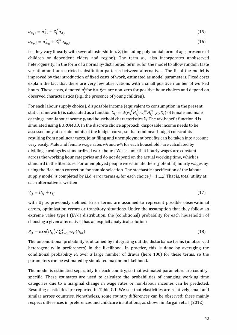
40

7cd� = 7cd8 + l�f7cd (15)

7cg� = 7cg8 + l�h7cg , (16)

i.e. they vary linearly with several taste-shifters Zi (including polynomial form of age, presence of

children or dependent elders and region). The term 7E� also incorporates unobserved

heterogeneity, in the form of a normally-distributed term ui, for the model to allow random taste

variation and unrestricted substitution patterns between alternatives. The fit of the model is

improved by the introduction of fixed costs of work, estimated as model parameters. Fixed costs

explain the fact that there are very few observations with a small positive number of worked

hours. These costs, denoted k-*for k = f;m, are non-zero for positive hour choices and depend on

observed characteristics (e.g., the presence of young children).

For each labour supply choice j, disposable income (equivalent to consumption in the present

static framework) is calculated as a function ��- = n(S�fe�-

f , S�he�-h, o� , ��) of female and male

earnings, non-labour income yi and household characteristics Xi. The tax-benefit function d is

simulated using EUROMOD. In the discrete choice approach, disposable income needs to be

assessed only at certain points of the budget curve, so that nonlinear budget constraints

resulting from nonlinear taxes, joint filing and unemployment benefits can be taken into account

very easily. Male and female wage rates wfi and wm

i for each household i are calculated by

dividing earnings by standardized work hours. We assume that hourly wages are constant

across the working hour categories and do not depend on the actual working time, which is

standard in the literature. For unemployed people we estimate their (potential) hourly wages by

using the Heckman correction for sample selection. The stochastic specification of the labour

supply model is completed by i.i.d. error terms eij for each choice j = 1;…;J. That is, total utility at

each alternative is written

p�- = K�- + q�- (17)

with Uij as previously defined. Error terms are assumed to represent possible observational

errors, optimization errors or transitory situations. Under the assumption that they follow an

extreme value type I (EV-I) distribution, the (conditional) probability for each household i of

choosing a given alternative j has an explicit analytical solution:

��- = rsN;K�->/∑ rsN(K�*)u*./ (18)

The unconditional probability is obtained by integrating out the disturbance terms (unobserved

heterogeneity in preferences) in the likelihood. In practice, this is done by averaging the

conditional probability Pij over a large number of draws (here 100) for these terms, so the

parameters can be estimated by simulated maximum likelihood.

The model is estimated separately for each country, so that estimated parameters are country-

specific. These estimates are used to calculate the probabilities of changing working time

categories due to a marginal change in wage rates or non-labour incomes can be predicted.

Resulting elasticities are reported in Table C.1. We see that elasticities are relatively small and

similar across countries. Nonetheless, some country differences can be observed: these mainly

respect differences in preferences and childcare institutions, as shown in Bargain et al. (2012).

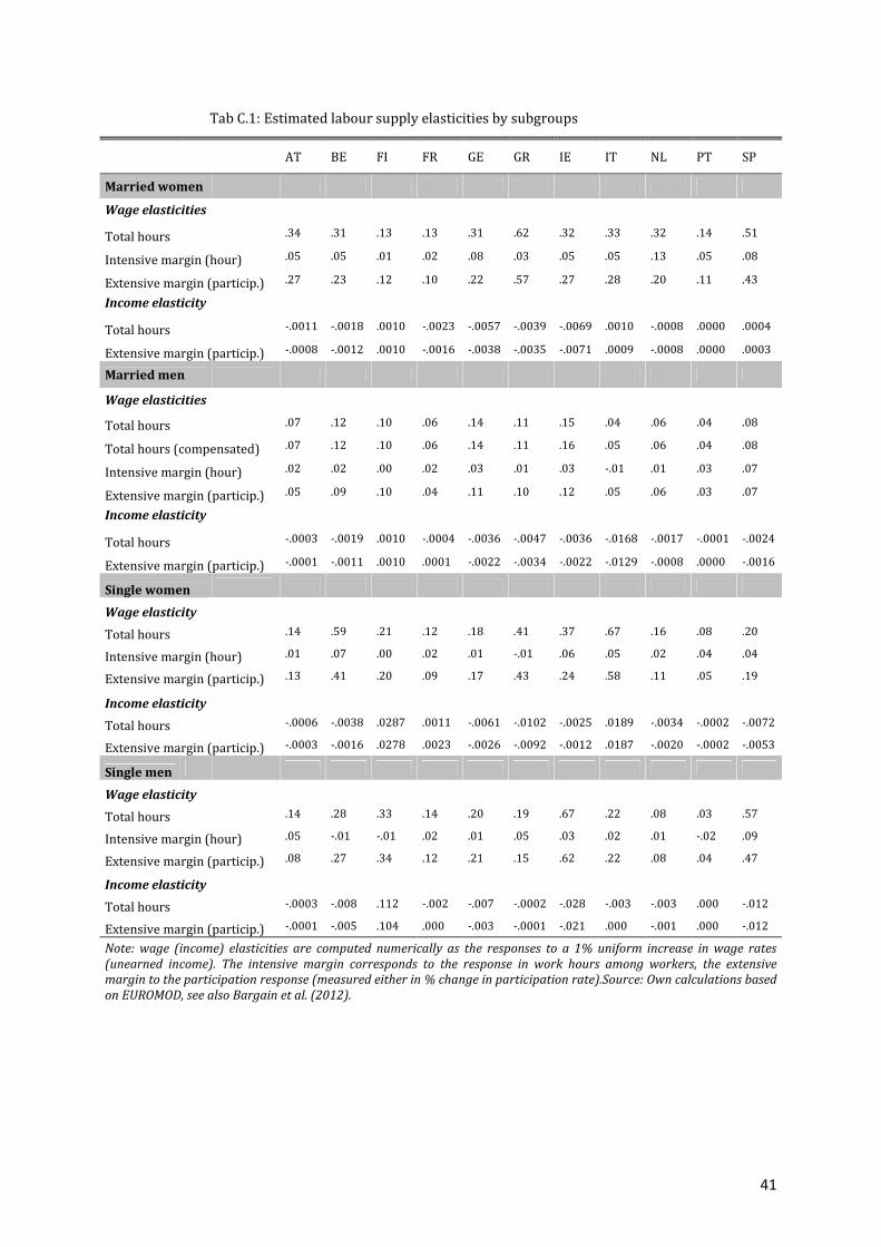
41

Tab C.1: Estimated labour supply elasticities by subgroups

AT BE FI FR GE GR IE IT NL PT SP

Married women

Wage elasticities

Total hours .34 .31 .13 .13 .31 .62 .32 .33 .32 .14 .51

Intensive margin (hour) .05 .05 .01 .02 .08 .03 .05 .05 .13 .05 .08

Extensive margin (particip.) .27 .23 .12 .10 .22 .57 .27 .28 .20 .11 .43

Income elasticity

Total hours -.0011 -.0018 .0010 -.0023 -.0057 -.0039 -.0069 .0010 -.0008 .0000 .0004

Extensive margin (particip.) -.0008 -.0012 .0010 -.0016 -.0038 -.0035 -.0071 .0009 -.0008 .0000 .0003

Married men

Wage elasticities

Total hours .07 .12 .10 .06 .14 .11 .15 .04 .06 .04 .08

Total hours (compensated) .07 .12 .10 .06 .14 .11 .16 .05 .06 .04 .08

Intensive margin (hour) .02 .02 .00 .02 .03 .01 .03 -.01 .01 .03 .07


Income elasticity

Total hours -.0003 -.0019 .0010 -.0004 -.0036 -.0047 -.0036 -.0168 -.0017 -.0001 -.0024

Extensive margin (particip.) -.0001 -.0011 .0010 .0001 -.0022 -.0034 -.0022 -.0129 -.0008 .0000 -.0016

Single women

Wage elasticity

Total hours .14 .59 .21 .12 .18 .41 .37 .67 .16 .08 .20

Intensive margin (hour) .01 .07 .00 .02 .01 -.01 .06 .05 .02 .04 .04


Income elasticity

Total hours -.0006 -.0038 .0287 .0011 -.0061 -.0102 -.0025 .0189 -.0034 -.0002 -.0072

Extensive margin (particip.) -.0003 -.0016 .0278 .0023 -.0026 -.0092 -.0012 .0187 -.0020 -.0002 -.0053

Single men

Wage elasticity

Total hours .14 .28 .33 .14 .20 .19 .67 .22 .08 .03 .57

Intensive margin (hour) .05 -.01 -.01 .02 .01 .05 .03 .02 .01 -.02 .09


Income elasticity

Total hours -.0003 -.008 .112 -.002 -.007 -.0002 -.028 -.003 -.003 .000 -.012

Extensive margin (particip.) -.0001 -.005 .104 .000 -.003 -.0001 -.021 .000 -.001 .000 -.012

Note: wage (income) elasticities are computed numerically as the responses to a 1% uniform increase in wage rates

(unearned income). The intensive margin corresponds to the response in work hours among workers, the extensive

margin to the participation response (measured either in % change in participation rate).Source: Own calculations based

on EUROMOD, see also Bargain et al. (2012).

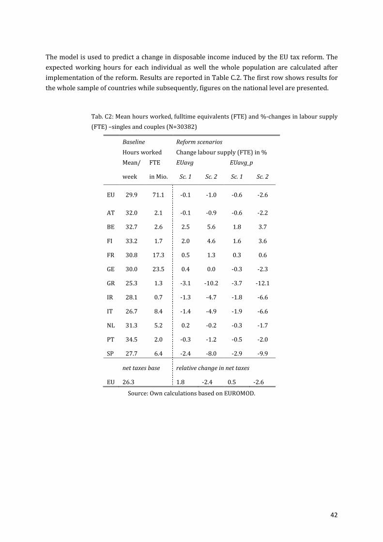
42

The model is used to predict a change in disposable income induced by the EU tax reform. The

expected working hours for each individual as well the whole population are calculated after

implementation of the reform. Results are reported in Table C.2. The first row shows results for

the whole sample of countries while subsequently, figures on the national level are presented.

Tab. C2: Mean hours worked, fulltime equivalents (FTE) and %-changes in labour supply

(FTE) –singles and couples (N=30382)

Baseline

Hours worked

Reform scenarios

Change labour supply (FTE) in %

Mean/ FTE EUavg EUavg_p

week in Mio. Sc. 1 Sc. 2 Sc. 1 Sc. 2

EU 29.9 71.1 -0.1 -1.0 -0.6 -2.6

AT 32.0 2.1 -0.1 -0.9 -0.6 -2.2

BE 32.7 2.6 2.5 5.6 1.8 3.7

FI 33.2 1.7 2.0 4.6 1.6 3.6

FR 30.8 17.3 0.5 1.3 0.3 0.6

GE 30.0 23.5 0.4 0.0 -0.3 -2.3

GR 25.3 1.3 -3.1 -10.2 -3.7 -12.1

IR 28.1 0.7 -1.3 -4.7 -1.8 -6.6

IT 26.7 8.4 -1.4 -4.9 -1.9 -6.6

NL 31.3 5.2 0.2 -0.2 -0.3 -1.7

PT 34.5 2.0 -0.3 -1.2 -0.5 -2.0

SP 27.7 6.4 -2.4 -8.0 -2.9 -9.9

net taxes base relative change in net taxes

EU 26.3 1.8 -2.4 0.5 -2.6


43

Tab. C.3: Fulltime equivalents (FTE) and %-changes (FTE) –single men and women

Single men Single women

EUavg EUavg_p EUavg EUavg_p

SQ Sc.1 Sc.2 Sc.1 Sc.2 SQ Sc.1 Sc.2 Sc.1 Sc.2

EU 7.8 0.3 -1.3 -0.4 -3.7 8.1 0.5 0.4 -0.3 -2.2

AT 0.3 0.8 1.8 0.5 0.9 0.3 0.6 0.8 0.1 -0.9

BE 0.2 6.0 9.6 5.3 7.9 0.2 7.7 17.5 6.2 14.1

FI 0.2 5.3 13.5 4.5 11.4 0.2 3.0 7.7 2.5 6.5

FR 1.6 2.6 6.1 2.2 5.0 2.0 2.5 7.6 2.2 6.7

GE 3.5 -0.4 -3.4 -1.3 -6.6 3.2 0.4 -0.3 -0.7 -3.8

GR 0.1 -1.4 -4.8 -1.7 -5.8 0.1 -9.7 -27.9 -11.0 -31.5

IR 0.1 -1.7 -8.0 -3.1 -12.4 0.1 -1.3 -5.1 -2.1 -7.8

IT 0.6 -1.1 -3.6 -1.7 -5.6 0.7 -3.9 -13.4 -5.2 -18.0

NL 0.5 1.3 2.6 1.0 1.8 0.5 2.5 6.1 2.0 4.6

PT 0.1 -0.1 -1.4 -0.4 -2.3 0.2 -1.6 -5.3 -2.1 -7.0

SP 0.6 -4.9 -18.9 -6.3 -23.9 0.6 -3.2 -11.4 -3.8 -13.7


Tab. C.4: Fulltime equivalents (FTE) and %-changes–married men and women

Married men Married women

EUavg EUavg_p EUavg EUavg_p

SQ Sc.1 Sc.2 Sc.1 Sc.2 SQ Sc.1 Sc.2 Sc.1 Sc.2

EU 37.4 0.0 -0.3 -0.8 -0.4 17.8 -0.5 -1.9 -1.1 -3.7

AT 1.1 0.2 0.2 0.2 -0.2 0.5 -1.9 -6.0 -2.7 -8.4

BE 1.4 1.6 2.8 3.8 1.0 0.8 1.6 4.1 0.8 1.7

FI 0.7 1.7 2.9 3.8 1.3 0.5 0.8 1.1 0.6 0.6

FR 8.7 0.1 0.1 0.0 -0.1 5.0 -0.1 -0.5 -0.4 -1.2

GE 11.2 0.6 0.9 0.9 0.1 5.5 0.5 0.5 -0.2 -1.6

GR 0.9 -1.8 -4.0 -6.7 -2.2 0.3 -5.3 -15.8 -6.3 -18.7

IR 0.4 -0.6 -1.4 -2.4 -0.9 0.2 -2.7 -8.8 -3.2 -10.8

IT 5.1 -1.1 -2.5 -4.1 -1.4 2.0 -1.4 -4.5 -2.1 -6.7

NL 2.9 0.0 -0.2 -0.6 -0.4 1.3 -0.8 -2.9 -1.7 -5.5

PT 1.1 -0.1 -0.3 -0.6 -0.3 0.7 -0.4 -1.3 -0.6 -2.1

SP 4.0 -1.2 -2.6 -4.3 -1.5 1.2 -4.5 -13.5 -5.6 -16.5


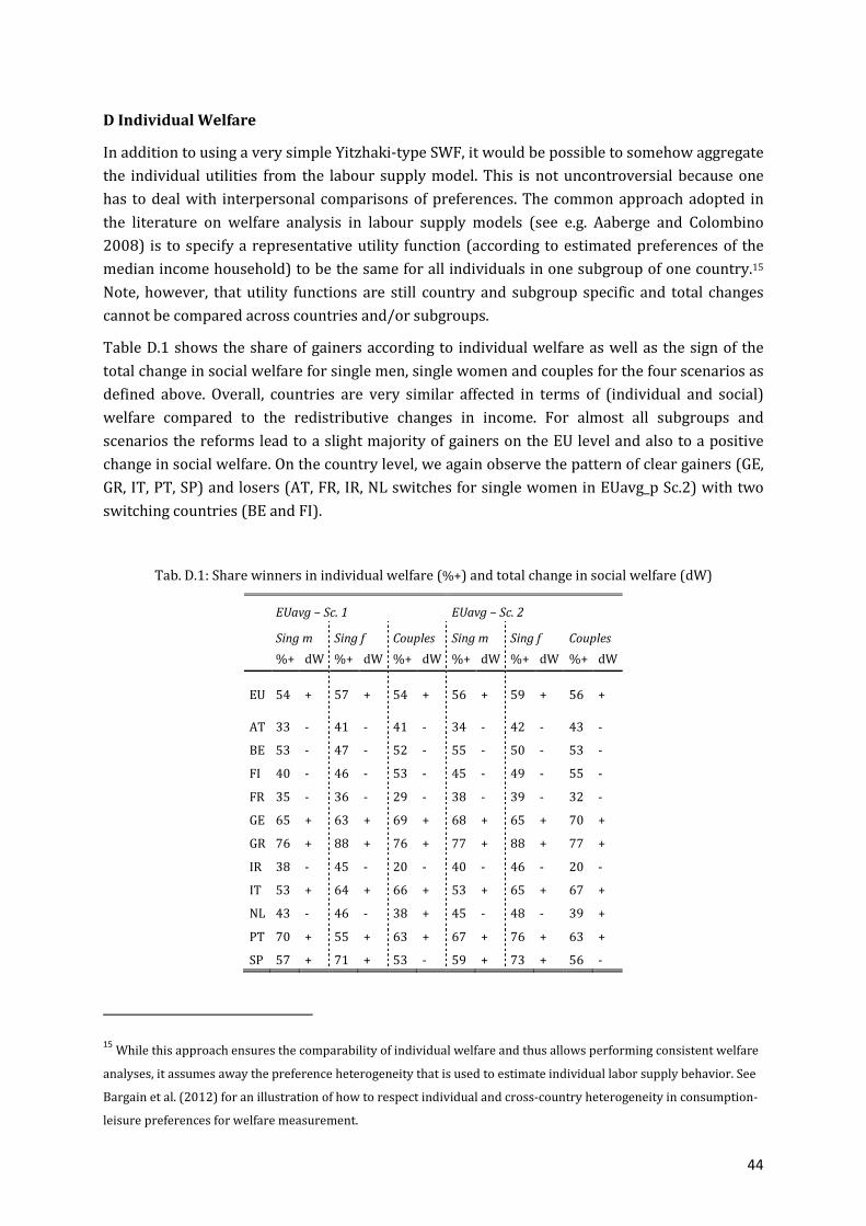
44

D Individual Welfare

In addition to using a very simple Yitzhaki-type SWF, it would be possible to somehow aggregate

the individual utilities from the labour supply model. This is not uncontroversial because one

has to deal with interpersonal comparisons of preferences. The common approach adopted in

the literature on welfare analysis in labour supply models (see e.g. Aaberge and Colombino

2008) is to specify a representative utility function (according to estimated preferences of the

median income household) to be the same for all individuals in one subgroup of one country.15

Note, however, that utility functions are still country and subgroup specific and total changes

cannot be compared across countries and/or subgroups.

Table D.1 shows the share of gainers according to individual welfare as well as the sign of the

total change in social welfare for single men, single women and couples for the four scenarios as

defined above. Overall, countries are very similar affected in terms of (individual and social)

welfare compared to the redistributive changes in income. For almost all subgroups and

scenarios the reforms lead to a slight majority of gainers on the EU level and also to a positive

change in social welfare. On the country level, we again observe the pattern of clear gainers (GE,

GR, IT, PT, SP) and losers (AT, FR, IR, NL switches for single women in EUavg_p Sc.2) with two

switching countries (BE and FI).

Tab. D.1: Share winners in individual welfare (%+) and total change in social welfare (dW)

EUavg – Sc. 1 EUavg – Sc. 2

Sing m Sing f Couples Sing m Sing f Couples

%+ dW %+ dW %+ dW %+ dW %+ dW %+ dW

EU 54 + 57 + 54 + 56 + 59 + 56 +

AT 33 - 41 - 41 - 34 - 42 - 43 -

BE 53 - 47 - 52 - 55 - 50 - 53 -

FI 40 - 46 - 53 - 45 - 49 - 55 -

FR 35 - 36 - 29 - 38 - 39 - 32 -

GE 65 + 63 + 69 + 68 + 65 + 70 +

GR 76 + 88 + 76 + 77 + 88 + 77 +

IR 38 - 45 - 20 - 40 - 46 - 20 -

IT 53 + 64 + 66 + 53 + 65 + 67 +

NL 43 - 46 - 38 + 45 - 48 - 39 +

PT 70 + 55 + 63 + 67 + 76 + 63 +

SP 57 + 71 + 53 - 59 + 73 + 56 -

15 While this approach ensures the comparability of individual welfare and thus allows performing consistent welfare

analyses, it assumes away the preference heterogeneity that is used to estimate individual labor supply behavior. See

Bargain et al. (2012) for an illustration of how to respect individual and cross-country heterogeneity in consumption-

leisure preferences for welfare measurement.

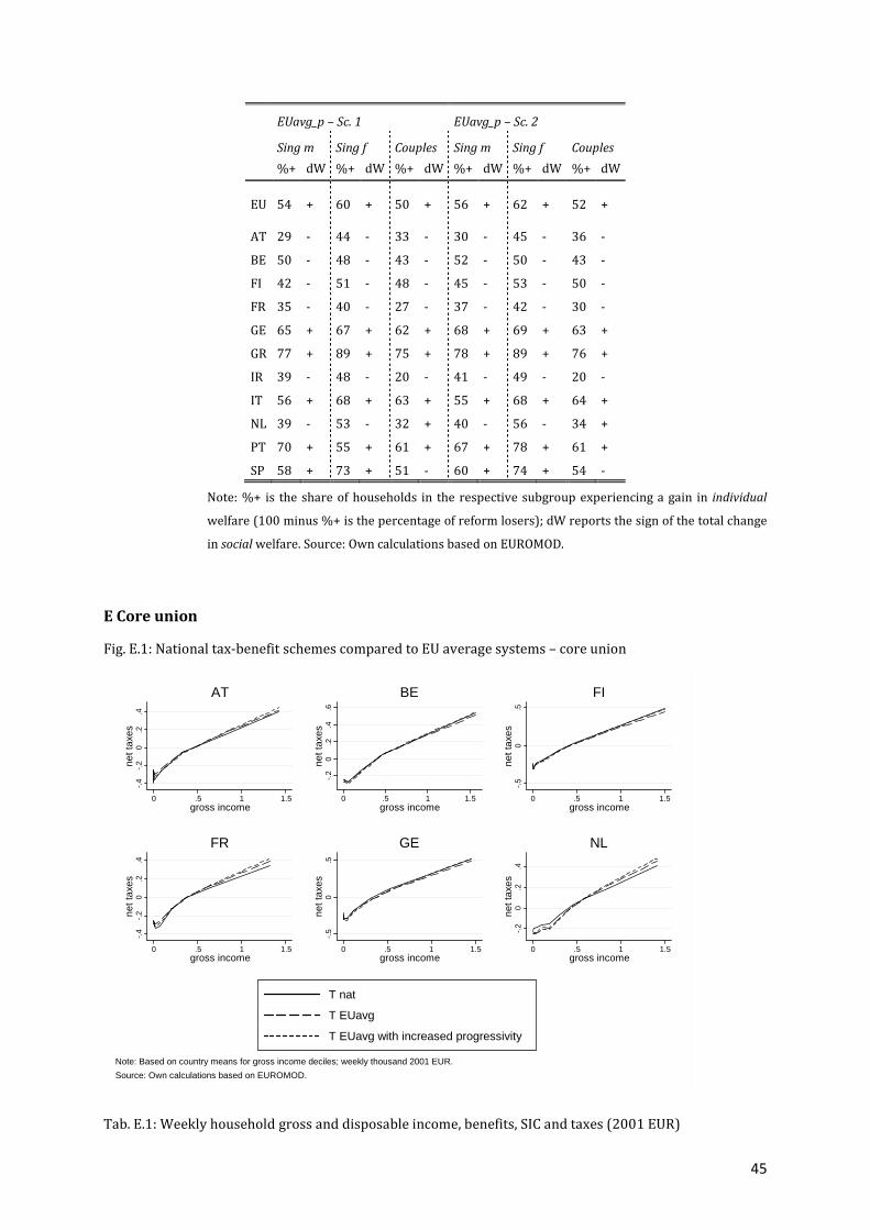
45

EUavg_p – Sc. 1 EUavg_p – Sc. 2

Sing m Sing f Couples Sing m Sing f Couples

%+ dW %+ dW %+ dW %+ dW %+ dW %+ dW

EU 54 + 60 + 50 + 56 + 62 + 52 +

AT 29 - 44 - 33 - 30 - 45 - 36 -

BE 50 - 48 - 43 - 52 - 50 - 43 -

FI 42 - 51 - 48 - 45 - 53 - 50 -

FR 35 - 40 - 27 - 37 - 42 - 30 -

GE 65 + 67 + 62 + 68 + 69 + 63 +

GR 77 + 89 + 75 + 78 + 89 + 76 +

IR 39 - 48 - 20 - 41 - 49 - 20 -

IT 56 + 68 + 63 + 55 + 68 + 64 +

NL 39 - 53 - 32 + 40 - 56 - 34 +

PT 70 + 55 + 61 + 67 + 78 + 61 +

SP 58 + 73 + 51 - 60 + 74 + 54 -

Note: %+ is the share of households in the respective subgroup experiencing a gain in individual

welfare (100 minus %+ is the percentage of reform losers); dW reports the sign of the total change

in social welfare. Source: Own calculations based on EUROMOD.

E Core union

Fig. E.1: National tax-benefit schemes compared to EU average systems – core union

Tab. E.1: Weekly household gross and disposable income, benefits, SIC and taxes (2001 EUR)

-.4

-.2

0.2

.4ne

t tax

es


AT

-.2

0.2

.4.6

net t

axes


BE

-.5

0.5

net t

axes


FI

-.4

-.2

0.2

.4ne

t tax

es


FR

-.5

0.5

net t

axes


GE

-.2

0.2

.4ne

t tax

es


NL

Note: Based on country means for gross income deciles; weekly thousand 2001 EUR.


T nat

T EUavg


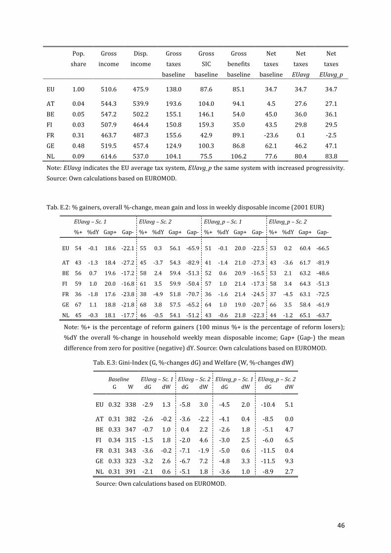
46

Pop.

share

Gross

income

Disp.

income

Gross

taxes

baseline

Gross

SIC

baseline

Gross

benefits

baseline

Net

taxes

baseline

Net

taxes

EUavg

Net

taxes

EUavg_p

EU 1.00 510.6 475.9 138.0 87.6 85.1 34.7 34.7 34.7

AT 0.04 544.3 539.9 193.6 104.0 94.1 4.5 27.6 27.1

BE 0.05 547.2 502.2 155.1 146.1 54.0 45.0 36.0 36.1

FI 0.03 507.9 464.4 150.8 159.3 35.0 43.5 29.8 29.5

FR 0.31 463.7 487.3 155.6 42.9 89.1 -23.6 0.1 -2.5

GE 0.48 519.5 457.4 124.9 100.3 86.8 62.1 46.2 47.1

NL 0.09 614.6 537.0 104.1 75.5 106.2 77.6 80.4 83.8

Note: EUavg indicates the EU average tax system, EUavg_p the same system with increased progressivity.


Tab. E.2: % gainers, overall %-change, mean gain and loss in weekly disposable income (2001 EUR)



EU 54 -0.1 18.6 -22.1 55 0.3 56.1 -65.9 51 -0.1 20.0 -22.5 53 0.2 60.4 -66.5

AT 43 -1.3 18.4 -27.2 45 -3.7 54.3 -82.9 41 -1.4 21.0 -27.3 43 -3.6 61.7 -81.9

BE 56 0.7 19.6 -17.2 58 2.4 59.4 -51.3 52 0.6 20.9 -16.5 53 2.1 63.2 -48.6

FI 59 1.0 20.0 -16.8 61 3.5 59.9 -50.4 57 1.0 21.4 -17.3 58 3.4 64.3 -51.3

FR 36 -1.8 17.6 -23.8 38 -4.9 51.8 -70.7 36 -1.6 21.4 -24.5 37 -4.5 63.1 -72.5

GE 67 1.1 18.8 -21.8 68 3.8 57.5 -65.2 64 1.0 19.0 -20.7 66 3.5 58.4 -61.9

NL 45 -0.3 18.1 -17.7 46 -0.5 54.1 -51.2 43 -0.6 21.8 -22.3 44 -1.2 65.1 -63.7




Tab. E.3: Gini-Index (G, %-changes dG) and Welfare (W, %-changes dW)

Baseline EUavg – Sc. 1 EUavg – Sc. 2 EUavg_p – Sc. 1 EUavg_p – Sc. 2

G W dG dW dG dW dG dW dG dW

EU 0.32 338 -2.9 1.3 -5.8 3.0 -4.5 2.0 -10.4 5.1

AT 0.31 382 -2.6 -0.2 -3.6 -2.2 -4.1 0.4 -8.5 0.0

BE 0.33 347 -0.7 1.0 0.4 2.2 -2.6 1.8 -5.1 4.7

FI 0.34 315 -1.5 1.8 -2.0 4.6 -3.0 2.5 -6.0 6.5

FR 0.31 343 -3.6 -0.2 -7.1 -1.9 -5.0 0.6 -11.5 0.4

GE 0.33 323 -3.2 2.6 -6.7 7.2 -4.8 3.3 -11.5 9.3

NL 0.31 391 -2.1 0.6 -5.1 1.8 -3.6 1.0 -8.9 2.7


Oxford University Centre for Business

Taxation

Working Paper series

WP12/21 Peter Egger, Christian Keuschnigg, Valeria Merlo and

Georg Wamser Corporate taxes and internal borrowing within

multinational firms

WP12/20 Jarkko Harju and Tuomos Kosonen The impact of tax

incentives on the economic activity of entrepreneurs

WP12/19 Laura Kawano and Joel slemrod The effects of tax rates

and tax bases on corporate tax revenues: estimates with new

measures of the corporate tax base

WP12/18 Giacomo Rodano, Nicolas Serrano-Velarde and

Emanuele Tarantino Bankruptcy law and the cost of banking

finance

WP12/17 Xavier Boutin, Giacinta Cestone, Chiara Fumagalli,

Giovanni Pica and Nicolas Serrano-Velarde The Deep pocket

effect of internal capital markets

WP12/16 Clemens Fuest, Andreas Peichl and Sebastian Siegloch

Which workers bear the burden of corporate taxation and

which firms can pass it on? Micro evidence from Germany

WP12/15 Michael P. Devereux Issues in the Design of Taxes on

Corporate Profit

WP12/14 Alan Auerbach and Michael P. Devereux Consumption

Taxes In An International Setting

WP12/13 Wiji Arulampalam, Michael P. Devereux and Federica

Liberini Taxes and the location of targets

WP12/12 Scott Dyreng, Bradley Lindsey and Jacob Thornock

Exploring the role Delaware plays as a tax haven

WP12/11 Katarzyna Bilicka and Clemens Fuest With which

countries do tax havens share information?

WP12/10 Giorgia Maffini Territoriality, Worldwide Principle,

and Competitiveness of Multinationals: A Firm-level Analysis of

Tax Burdens

WP12/09 Daniel Shaviro The rising tax-electivity of US residency

WP12/08 Edward D Kleinbard Stateless Income

WP12/07 Vilen Lipatov and Alfons Weichenrieder Optimal income

taxation with tax competition

WP12/06 Kevin S Markle A Comparison of the Tax-motivated

Income Shifting of Multinationals in Territorial and

Worldwide Countries

WP12/05 Li Liu Income Taxation and Business Incorporation:

Evidence from the Early Twentieth Century

WP12/04 Shafik Hebous and Vilen Lipatov A Journey from a

Corruption Port to a Tax Haven

WP12/03 Neils Johannesen Strategic line drawing between debt

and equity

WP12/02 Chongyang Chen, Zhonglan Dai, Douglas A.

Shackelford and Harold H. Zhang, Does Financial Constraint

Affect Shareholder Taxes and the Cost of Equity Capital?

WP12/01 Stephen R. Bond and Irem Guceri, Trends in UK BERD

after the Introduction of R&D Tax Credits

WP11/24 Michael Devereux and Simon Loretz How would EU

corporate tax reform affect US investment in Europe?

WP11/23 Krautheim, Sebastian and Tim Schmidt-Eisenlohr

Wages and International Tax Competition

WP11/22 Haufler, Andreas, Pehr-Johan Nörback and Lars

Persson Entrepreneurial innovation and taxation

WP11/21 Mancini, Raffaele, Paolo M. Panteghini and Maria laura

Parisi Debt-Shifting in Europe

WP11/20 Xing, Jing Does tax structure affect economic growth?

Empirical evidence from OECD countries

WP11/19 Freedman, Judith Responsive regulation, risk and rules:

applying the theory to tax practice

WP11/18 Devereux, Michael P. and Simon Loretz How would EU

corporate tax reform affect US investment in Europe?

WP11/17 Vella, John, Clemens Fuest and Tim Schmidt-Eisenlohr

Response on EU proposal for a Financial Transaction Tax

WP11/16 Loretz, Simon and Socrates Mokkas Evidence for

profit-shifting with tax sensitive capital stocks

WP11/15 Weisenbach, david A. Carbon taxation in the EU:

Expanding EU carbon price

WP11/14 Bauer, Christian, Davies, Ronald B. and Andreas Hauer

Economic Integration and the Optimal Corporate Tax

Structure with Heterogeneous Firms

WP11/13 Englisch, Joachim National Measures to Counter Tax

Avoidance under the Merger Directive

WP11/12 de la Feria, Rita and Clemens Fuest Closer to an

Internal Market? The Economic Effects of EU Tax Jurisprudence

WP11/11 Englisch, Joachim EU Perspective on VAT Exemptions

WP11/10 Riedel, Nadine and Hannah Schildberg-Hörisch

Asymmetric Obligations

WP11/09 Böhm, Tobias and Nadine Riedel On Selection into

Public Civil Service

WP11/08 Auerbach, Alan J. and Michael P. Devereux Consumption

and Cash-Flow Taxes in an International Setting

WP11/07 Becker, Johannes and Clemens Fuest Tax Competition:

M&A versus Greenfield Investment

WP11/06 Riedel, Nadine Taxing Multinationals under Union

Wage Bargaining

WP11/05 Liu, Li and Rosanne Altshuler Measuring the Burden of

the Corporate Income Tax under Imperfect Competition

WP11/04 Becker, Johannes and Clemens Fuest The Taxation of

Foreign Profits - The Old View, the New View, and a Pragmatic

View

WP11/03 Konrad, Kai Search Costs and Corporate Income Tax

Competition

WP11/02 Hellerstein,Walter Comparing the Treatment of

Charities Under Value Added Taxes and Retail Sales Taxes

WP11/01 Dharmapala, Dhammika and Nadine Riedel Earnings

Shocks and Tax-Motivated Income-Shifting: Evidence from

European Multinationals

WP10/23 Schmidt-Eisenlohr, Tim Towards a Theory of Trade

Finance

WP10/22 Freedman, Judith and John Vella HMRC's Management

of the UK Tax System: The Boundaries of Legitimate Discretion

WP10/21 de la Feria, Rita Reverberation of Legal Principles:

Further Thoughts on the Development of an EU Principle of

Prohibition of Abuse of Law

WP10/20 Hauer, Andreas and Frank Stähler Tax competition in a

simple model with heterogeneous firms: How larger markets

reduce profit taxes

WP10/19 Cnossen, Sijbren Improving the VAT Treatment of

Exempt Immovable Property in the European Union

WP10/18 Grubert, Harry and Richard Krever VAT and Financial

Supplies: What should be taxed?

WP10/17 Gendron, Pierre-Pascal VAT Treatment of Public Sector

Bodies: The Canadian Model

WP10/16 Niepmann, Friederike and Tim Schmidt-Eisenlohr Bank

Bailouts, International Linkages and Cooperation

WP10/15 Bond, Stephen and Jing Xing Corporate taxation and

capital accumulation

WP10/14 Lockwood, Ben How should financial intermediation

services be taxed?

WP10/13 Becker, Johannes, Fuest, Clemens and Nadine Riedel

Corporate tax effects on the quality and quantity of FDI

WP10/12 Fuest, Clemens and Nadine Riedel Tax Evasion and Tax

Avoidance in Developing Countries: The Role of International

Profit Shifting

WP10/11 Wildasin, David E. State Corporation Income Taxation:

An Economic Perspective on Nexus

WP10/10 Becker, Johannes and Marco Runkel Corporate tax

regime and international allocation of ownership

WP10/09 Simpson, Helen How do firms' outward FDI strategies

relate to their activity at home? Empirical evidence for the UK

WP10/08 Voget, Johannes, Headquarter Relocations and

International Taxation

WP10/07 Devereux, Michael P. and Simon Loretz Evaluating

Neutrality Properties of Corporate Tax Reforms

WP10/06 Davies, Ronald B. and Lourenço S. Paz, Tarifs Versus VAT

in the Presence of Heterogeneous Firms and an Informal Sector

WP10/05 Finke, Katharina, Heckemeyer, Jost H., Reister Timo and

Christoph Spengel Impact of Tax Rate Cut Cum Base Broadening

Reforms on Heterogeneous Firms - Learning from the German

Tax Reform 2008

WP10/04 Koh, Hyun-Ju and Nadine Riedel Do Governments Tax

Agglomeration Rents?

WP10/03 Dischinger, Matthias and Nadine Riedel The Role of

Headquarters in Multinational Profit Shifting Strategies

WP10/02 Vrijburg, Hendrik and Ruud A. de Mooij Enhanced

Cooperation in an asymmetric model of Tax Competition

WP10/01 Bettendorf, Leon, van der Horst Albert, de Mooij, Ruud

A. and Hendrik

Vrijburg, Corporate tax consolidation and enhanced

cooperation in the European Union

WP09/32 Bettendorf, Leon, Devereux, Michael P., van der Horst,

Albert, Loretz,

Simon and Ruud A. de Mooij Corporate tax harmonization in

the EU

WP09/31 Karkinsky, Tom and Nadine Riedel Corporate Taxation

and the Choice

of Patent Location within Multinational Firms

WP09/30 Becker, Johannes and Clemens Fuest Transfer Pricing

Policy and the

Intensity of Tax Rate Competition

fiscal union in europe? redistributive and stabilising ... · fiscal union in europe?...

Documents