WORKING PAPER SERIESNO 1472 / SEPTEMBER 2012

FISCAL SUSTAINABILITY USING GROWTH-MAXIMISING

DEBT TARGETS

Cristina D. Checherita-Westphal, Andrew Hughes Hallett and Philipp C. Rother

NOTE: This Working Paper should not be reported as representing the views of the European Central Bank (ECB). The views expressed are

those of the authors and do not necessarily reflect those of the ECB.

© European Central Bank, 2012

AddressKaiserstrasse 29, 60311 Frankfurt am Main, Germany

Postal addressPostfach 16 03 19, 60066 Frankfurt am Main, Germany

Telephone+49 69 1344 0

Internethttp://www.ecb.europa.eu

Fax+49 69 1344 6000

All rights reserved.

ISSN 1725-2806 (online)

Any reproduction, publication and reprint in the form of a different publication, whether printed or produced electronically, in whole or in part, is permitted only with the explicit written authorisation of the ECB or the authors.

This paper can be downloaded without charge from http://www.ecb.europa.eu or from the Social Science Research Network electronic library at http://ssrn.com/abstract_id=2145281.

Information on all of the papers published in the ECB Working Paper Series can be found on the ECB’s website, http://www.ecb.europa.eu/pub/scientific/wps/date/html/index.en.html

AcknowledgementsThe views expressed in this paper are exclusively those of the authors and do not necessarily reflect those of the European Central Bank. We are grateful to Martin Zagler, Michel Julliard, as well as to participants of the Banque de France and BETA Conference on Macroeconomic and Financial Vulnerability Indicators in Advanced Eeconomies, Strasbourg, September 2012, and in particular to our discussant, Lukas Reiss, for useful comments. Special thanks go to Roberta De Stefani for her excellent research assistance in using the OECD Analytical database (OED).

Cristina D. Checherita-Westphalat European Central Bank, Kaiserstrasse 29, D-60311 Frankfurt am Main, Germany; e-mail: cristina.checherita-westphal@ecb.europa.eu

Andrew Hughes Hallettat Harvard Kennedy School, 79 John F. Kennedy Street, Cambridge, MA 02138 USA and School of Public Policy, George Mason University, 3351 Fairfax Dr., Arlington VA 22201, USA; e-mail: ahughesh@gmu.edu

Philipp C. Rotherat European Central Bank, Kaiserstrasse 29, D-60311 Frankfurt am Main, Germany; e-mail: philipp.rother@ecb.europa.eu

1

Abstract

This paper highlights the importance of debt-related fiscal rules and derives growth-maximising public debt ratios from a simple theoretical model. On the basis of evidence on the productivity of public capital, we estimate public debt targets that governments should try to maintain if they wish to maximise growth for panels of OECD, EU and euro area countries, respectively. These are not arbitrary numbers, as many of the fiscal rules in the literature suggest, but are founded on long-run optimising behaviour, assuming that governments implement the so-called golden rule over the cycle; that is, they contract debt only to finance public investment. Our estimates suggest that the euro area should target debt levels of around 50% of GDP if member states are to have common targets. That is about 15 percentage points lower than the estimate for the growth-maximising debt ratio in our OECD sample and comfortably within the Stability and Growth Pact’s debt ceiling of 60% of GDP. We also indicate how forward looking budget reaction functions fit into a debt targeting framework.

Keywords: Public debt, public capital, economic growth

JEL Classification: H63, E22, O40

2

Non-technical summary The global financial crisis and the debt problems suffered by an increasing number of euro area economies

have made the need for a new fiscal framework to prevent unsustainable fiscal policies developing again a

top priority. This paper highlights the importance of debt-related fiscal rules and derives growth-maximising

public debt ratios from a simple theoretical model.

First, the paper outlines the characteristics of (optimal) debt targets and their potential advantages within a

fiscal rule framework. Because the target is a stock and therefore persistent, such a rule would: (i) focus on

the ultimate risk, unsustainable public finances; (ii) introduce flexibility into policymaking as it could

accommodate some short-term fluctuations in the fiscal balance; and (iii) give policy makers a greater

incentive to obey the rules to preserve their freedom of manoeuvre in the future, also allowing for a more

limited scope for data manipulation (stock versus annual flow data).

Second, building on existing literature, the paper presents a simple theoretical model and underlines the

assumptions necessary to derive optimal, in the sense of growth-maximising, public debt ratios. A central

assumption is that governments implement the so-called golden rule over the cycle. That is, they contract

debt only to finance public investment, while current spending is financed through current revenues, not

borrowing.

Third, on the basis of empirical evidence on the productivity of public capital, we estimate average growth-

maximising public debt targets for three samples of OECD, EU and euro area countries. To do so, we

reconstruct harmonised public and private capital stock series across 22 OECD economies for the period

1960-2010 (dataset available upon request) from a previous study. Then, we estimate the output productivity

of public capital using a production function approach and conduct a large number of robustness checks to

tackle some of the main methodological problems of the earlier literature. The paper thus provides the first

theoretically-based estimates of the debt ratios that governments should try to maintain if they wish to

maximise growth. Our estimates suggest that the euro area should target debt levels of around 50% of GDP if

member states are to have common targets. That is 15 percentage points lower than the estimate for the

optimal debt ratio in our OECD sample and 10 points lower than the Stability and Growth Pact’s debt ceiling

of 60% of GDP.

Our approach is based on a specific growth model and a golden rule financing assumption. Its estimation and

inference uncertainties relate, above all, to data misallocations in the estimates for public and private capital

stocks, in several countries in particular. As a result, given current primary data sources, we cannot derive

reliable individual country debt targets. On the other hand, these estimation and measurement errors are

mitigated, to a large extent, in a panel model, hence our approach of modelling common debt targets.

Finally, the paper also indicates how forward looking budget reaction functions fit into our debt targeting

framework and leaves an in-depth analysis in this area for further research.

3

1. Introduction

The global financial crisis and the debt problems suffered by an increasing number of euro area

economies have shown the urgency for new fiscal frameworks to prevent unsustainable fiscal

policies reoccurring. This paper highlights the importance of debt-related fiscal rules and derives

growth-maximising public debt ratios from a simple theoretical model.

Recent work (Reinhart and Rogoff 2010; Checherita and Rother 2010, Cecchetti et al. 2011, Baum

et al. 2012, among others) has identified nonlinear relationships between an economy’s debt burden

and its rate of growth. Such relationships imply an optimal, in the sense of growth-maximising,

level of debt. But because they are purely empirical, we have little idea what that optimal level of

debt depends upon; nor how to set an optimal level of debt in a particular fiscal regime and create a

safe zone so that public finances can remain sustainable in the face of unexpected shocks and

political uncertainty. Others have focused on the safe zone or “fiscal space” aspect, based on past

behaviour, by examining the fiscal limit or point at which fiscal policies become unsustainable and

public finances collapse (Ghosh et al. 2011). But an optimal level of debt has little meaning if fiscal

policies cannot be forced to stay within a safe zone below the fiscal limit. Equally, measuring the

fiscal limit is of little value if we cannot calculate the optimal debt level since it would only tell us

where we should not go, not what debt levels we should choose, or at least aim at. Moreover, given

the difficulties that many of the euro area countries have had in restraining their public debt, there is

little point constructing our fiscal framework on past behaviour.

This paper therefore takes the idea of a (possibly nonlinear) budget reaction function, and shows

how to calculate a growth-maximising steady state level of debt. We also provide the first numerical

estimates of theoretically determined-optimal debt ratios for three groups of countries: the OECD,

EU and euro area countries. These are not arbitrary numbers, as many of the fiscal rules in the

literature suggest, but are founded on long-run optimising behaviour, assuming that governments

contract debt only to finance investment.

We start by reviewing why debt targets, or protocols with specific enforcement conditions for

various debt ranges, could be considered superior to deficit targets or limits. The revised Stability

and Growth Pact (SGP), in force since late 2011, already includes fines on excess debt levels and a

rule for returning to acceptable debt limits, but no debt targets as such. The Report by the President

of the European Council of 26 June 2012 on proposals towards a genuine economic and monetary

union calls for effective mechanisms to prevent and correct unsustainable fiscal policies, inter alia,

4

by agreeing in common on upper limits on the annual budget balance and on government debt levels

of individual Member States. Subsequently, “the euro area level would be in a position to require

changes to budgetary envelopes if they are in violation of fiscal rules […].”

One justification for our approach derives from the natural inter-temporal policy assignments: fiscal

policies focus on long-term structural objectives and monetary policies on stabilisation issues. Debt

targets then provide a simple way to achieve such a set up. Given this framework, the paper uses a

simple theoretical model deriving the growth-maximising steady-state debt ratio. Based on this

model, and on a dataset for public capital stock (updated for the purpose), we estimate the average

growth-maximizing debt-to-GDP ratio for a panel of 22 OECD economies. We do the same for a

group of 13 largest EU and 11 euro area countries as a whole, to show what target values would be

needed if the system is to follow common debt targets. It turns out that the OECD would need debt

targets of about 67% of GDP, but the euro area would best operate with debt targets at 50% (not far

from, and comfortably below the Stability Pact’s 60% upper limit).

Drawbacks of our approach, including data limitations, are described in more details in Section 4.

Data issues currently preclude extending this analysis to reliable debt target estimates for individual

countries.

2. Why Target (Optimal) Debt Levels? There is by now an extensive literature on the need for and effectiveness of imposing fiscal limits,

and the different ways in which they may be imposed – not least in a currency union such as the

euro area. Many, if not most, of these studies concern themselves with an assessment of the

sustainability of fiscal policies/public finances (see European Economy 2011, part IV for an

extensive survey). There has also been a complementary discussion of fiscal rules (see, inter alia,

European Economy 2011, part III, for a survey). This discussion shows that the effectiveness of

imposing specific rules on the policy makers as a form of fiscal restraint depends on, first, the

enforcement mechanisms brought in to support those rules; and second, on the type of rule

imposed.2

2 Using a survey-based dataset on the EU fiscal framework, Debrun et al. (2008) find that budget balance and debt rules perform better than expenditure rules in terms of fiscal consolidation, but are also more frequently perceived to induce a pro-cyclicality bias. Several studies on the deficit rules (the most extensively studied or assumed fiscal rule) find that the ability of such rules to act as commitment devices, or as a defence against short sighted governments, or creative accounting (see, inter alia, von Hagen and Wolff, 2006 and Koen and Van den Noord, 2006) is rather uncertain. Buti et al. (2007) show that EU governments may have had an incentive to use creative accounting to paint their deficit rather (more) than debt in better shape, inter alia, using the stock-flow adjustment (DDA) variable. One of the reasons may

5

This literature is, however, not concerned with fiscal targets, that is, with what level of debt or

deficits countries would, or should, want to carry – as opposed to what levels they could tolerate

financially or economically; or what the determinants of these fiscal targets should be.

Our approach is to recognise that much of fiscal policy is concerned with longer term objectives.

This provides a natural opportunity to independently pre-commit fiscal policies (in the sense of a

Stackelberg game), in a way that can then be combined with independent monetary policies directed

at price stability and, if deemed desirable, short run demand management goals. That creates a basis

for rule-based coordination between policy-makers without the need for explicit negotiation: each

policy can operate according to comparative advantage. This opportunity for independent pre-

commitment arises from the fact that much of fiscal policy is usually committed to long run targets

(public services, social support, education, infrastructure, sustainable finances), and is not easily

reversible or easily used for discretionary stabilisation if consistency across time and policy types is

to be maintained.

The advantage of fiscal independence in this sense is that it allows us to create Pareto improvements

over the usual competitive policies without reducing the central bank’s ability to act independently

on shorter run objectives.3 But how to maintain that construct? Debt targets in this context have the

advantage of being a stock, not a flow. That introduces a degree of persistence, especially in

countries with higher levels of public debt. Debt targets can therefore be used to pre-commit or

anchor fiscal policies, the more so in countries that have been lax in the past, to a path which is

consistent with the expected stance of the independent monetary policy – and hence to achieve the

twin goals of sustainable public finances and limited spillovers on others.4

We contend that an overall debt ceiling combined with a fiscal adjustment rule would work better

for the following reasons.

First, such an approach introduces flexibility into policymaking: the pro-cyclicality of hard targets

that have to be achieved on an annual basis can be reduced, together with the tendency of rigid

targets to block structural reforms whenever the latter have short run fiscal costs. While this is in

principle also possible by using deficit rules, the focus on debt may make this target easier to

achieve. Thus, a debt ceiling combined with a suitably designed adjustment rule can accommodate

some short-term fluctuations in the fiscal balance.

have been that SGP rules had so far given considerably more attention to the deficit criterion rather than the debt criterion (see Buti et al., 2007). 3 See, for example, Dixit and Lambertini (2003), Hughes Hallett and Weymark (2007) and Hughes Hallett (2008a,b). 4 In Denmark, a policy of public debt targeting has been pursued for a decade (Andersen et al. 2008).

6

Further, debt limits, or debt targets, are helpful also because they focus on the ultimate risk:

unsustainable public finances. Moreover, the space between the debt target and the debt ceiling

allows policy-makers to trade off good years against bad. In effect, because the target is a stock not

a flow, this produces a (cyclically adjusted) structural rule without the difficulty of having to

calculate cyclically adjusted deficit figures accurately.5 Some space between the debt target and the

highest permitted value would then allow debt ratios to rise in bad years, but promote an automatic

return in good years (a primary surplus rule, rather than a balanced budget rule, being the

mechanism to achieve this). Pro-cyclicality can be thus avoided.

Finally, and again because the target is a stock and therefore persistent, a debt rule may give policy

makers a greater incentive to obey the rules: first, to preserve freedom of manoeuvre in the future;

second, to save at the top of the cycle and therefore remain “within target” in the future; third

because persistence in such a target makes it possible to create credibility and commitments for the

future, and finally, because meeting a stock fiscal target is less easily manipulable through “creative

accounting” compared to a flow target (see Hughes Hallett and Jensen, 2012), especially when

monitoring is done in real time (Hughes Hallett et al., 2012). From here we can get the fiscal pre-

commitment we need.

On the other hand, a fiscal regime that targets a debt ratio may still be subject to pro-cyclicality or

enforcement/monitoring problems. These include valuation effects for the foreign-currency

denominated debt share and other stock-flow adjustment operations, which may prove especially

burdensome in times of financial and economic stress (i.e. currency depreciation, debt-finance

support for acquisition of assets in economic sectors under stress, financial sector recapitalization

not reflected in the flow data). Moreover, the flexibility induced by a debt target - when the actual debt

ratio is well below the targeted one - may allow a government to run large deficits, leaving the binding

debt rule as a problem to its successor. To rule out the possibility of opportunistic behaviour by the

fiscal authorities, or a collapse through a loss of “fiscal capacity”, any debt targeting regime needs

to be accompanied by a minimum primary surplus/maximum primary deficit rule, an adequate “safe

zone” to handle unexpected shocks, and an enforcement mechanism.

Thus, a natural way to pre-commit fiscal policies in a way that can be combined with an

independent monetary policy, but without explicit negotiations, is to give fiscal policy an

independent capacity to decide for longer periods of commitment. To make this idea operational, we

5 For the significance of this point in terms of the missed or false alarms by the monitoring agency, and hence credibility lost by policy-makers, see Hughes Hallett et al. (2012).

7

give the fiscal authorities an optimal and explicit debt target for maximising growth (subject to

sustainability constraints on the public and the private sectors). That creates pre-commitment

derived from long-term objectives and a slow-moving target.

Fiscal-monetary coordination can now follow because, once the monetary authority knows what the

(now credible) long run path of fiscal policy is going to be, it is free to choose a monetary policy

that fits best in terms of its objectives. And should fiscal policy deviate from its chosen path,

monetary policies can quickly act to cut out any unwanted consequences. This threat, in the context

of a strategic policy game, should be enough to persuade fiscal policy-makers to stick with their

announced path.6 In fact, formal analysis shows exactly that. In asynchronous games, where policy

makers have different periods of commitment to their regime, and the policies which those regimes

generate, monetary discipline will constrain fiscal policies except in the most extreme cases (where

the central bank is impatient, or where its commitment relative to fiscal policy is insufficient).

However, this result could weaken in a monetary union depending on the number, size and ability of

the smaller economies to free ride on the discipline of others (Libich et al, 2012).

To guard against that possibility, one approach is to exploit the debt rules and sanctions available

within the new Stability and Growth Pact to enforce debt targets in cases of failure or fiscal fatigue.

In the latest revision of the Stability and Growth Pact, the emphasis on the debt level was

strengthened. Under the preventive arm, the Pact includes high debt ratios in the determination of

the so-called country specific medium-term budgetary objectives that countries are asked to achieve

to ensure sound budgetary positions. Moreover, if the current budgetary position falls short of the

medium-term objective, high-debt countries are to implement more ambitious adjustment plans to

achieve them. Under the corrective arm, for countries with debt ratios above the 60% of GDP

reference value an excessive deficit procedure can be launched if the debt ratio is deemed not to be

sufficiently diminishing and taking a number of additional factors into account. In particular, the

debt ratio should at least diminish annually by 1/20th of the distance between the actual debt ratio

and the 60% of GDP reference value.

3. Growth-maximising Debt – A Theoretical Framework The question of how to set specific debt target values remains. This might be done by adapting the

empirical results found so far in the literature on the links between public debt and output growth.

However, that kind of analysis is entirely empirical in its definition of the level of debt that

6 See Libich et al. (2012), and Libich and Stehlik (2008).

8

maximises growth rates. A theoretical explanation of why this link should exist, and how the debt

target should be determined, has not been attempted. In that regard, a more useful approach can be

derived from Aschauer’s (2000) model where the growth-optimising policy is expressed in terms of

the public-to-private capital ratios. This would allow us to determine and calculate the best level of

public debt – used exclusively for public capital financing - for any specific economy or sample

period. Such a policy implies a golden rule (or “debt brake”) in the long run since, over the cycle,

current government spending has to be financed by current revenues rather than borrowing.7 In

steady state, the debt ratio will then be constant over time – results later confirmed in the empirical

work of Aizenman et al. (2007). If maintained, such a rule would generate sufficient capital cover in

the economy as a whole for the public borrowing, which is just a matter of good banking practice.

How do we choose values for the optimal debt ratio to which we should converge? Taking the

Aschauer (2000) model as a starting point,8 we derive the level of public sector debt to maximise the

rate of economic growth as follows.

We start from a standard production function with public capital, with L= labour, K= private capital,

and gK = public capital (the accumulated stock of unfunded public spending). Borrowing is used to

fund that stock of public capital, whether it is productive or not. Thus:

1 1[ ] gY L K K (1)

Constant returns to scale are not always imposed. But they are needed here if optimal inputs are to

be defined under conditions of potentially unlimited borrowing.9 This model can be rewritten as:

1 ( / )gY L K K K (2)

where (1 ) ; and /gK K is the public to private capital ratio that defines the degree of public

sector borrowing. Think of it as the public sector input (e.g. infrastructure human capital) to the

production function. We need to estimate (2) because, given estimates of γ and α, the optimal level

of debt follows from the ratio of public to private capital that maximises the growth rate of output

per head at existing employment levels, defined as:

2(1 )

gK

K

= if L=1; or 1 2(1 )gK

L K

if not. (3)10

7 It might be thought that a debt target allows greater flexibility which governments might exploit to run large deficits, but imposing a debt brake/golden rule effectively rules this out since the rest of the budget has to be in balance. 8 Kamps (2005) also used this model to derive optimal public capital stock ratios in the OECD and EU. 9 Eq. (1) displays constant returns to scale overall, but also crucially between aggregate public and private sector inputs (and within private production). Without the second order conditions for a maximum, the search for growth will lead to steadily escalating debt - with financing costs as the only constraint. Default then becomes unavoidable.

9

This result is derived in Appendix 1. In either case the optimal debt ratio, d* = *

*

Y

K g , is:

d* =

1

2)1( (4)

Thus the optimal (long-run) level of debt, under golden rule conditions, just depends on the output

elasticity of public capital stock. Hence less productive forms of gK lead to lower values of , and

to lower optimal debt levels.

Commentary: We distinguish between the long run optimal level of debt when all capital and labour

ratios have settled at their optimal values, and short run optimal debt when those ratios are unable to

adjust or remain stuck at certain historical values. In the latter case, short run constrained optimal

debt will be 1* [ / ]d L K Y . The implication is that an economy with less private capital, and

hence less capital cover in relation to output, would have a lower optimal debt target in the short run

than in the long run. Thus those who substitute capital for labour to avoid high non-wage costs or

generous employment legislation will tend to have too high short run debt targets. Nonetheless, this

can only be a transitory state on the way to (4).

Why do we need a generalised model with flexible labour inputs? First, with the labour input

normalised, we cannot vary the labour to private and public capital ratios separately to get an

optimal mix of inputs, or an unconditional optimal public to private sector mix. That means we

could only correctly determine short run optimal debt ratios in the sense defined above – a matter of

some importance since short term ratios are only of interest for defining a transition path for

reducing current debt levels to their long run target level. Second, to define an optimal and finite

level of debt, we have to have constant returns to scale between the private and public sector inputs

as a whole – not just between private and public capital.

Finally, a drawback of this approach is that it relies on a specific growth model and a golden rule

financing assumption. The model also requires the use of public and private capital stock data,

which - despite offering better theoretical grounds - are subject to measurement errors, in particular

data misallocations in several country cases.

10 L is normalized to 1 in Aschauer (2000). More generally, (3) shows φ to be the optimal ratio of public to private inputs.

10

4. Growth-maximising Debt Ratios – Empirical Estimates 4.1 Estimating equations In order to calculate the steady-state debt ratios as derived in (4), we need to estimate the output

elasticity of public capital stock (α). Taking into account the relationships (1) and (2), we have three

options for estimating α:

1) Estimate the production function (1) directly, either in levels or growth rates; that is to regress lnY

on lnL, lnK and lnKg or their first differences (for individual countries constraint the coefficients of

the three explanatory variables to sum up to one);

2) Estimate the production function according to transformation (2), using data on the ratio Kg/K, by

regressing ln(Y/K) on ln(L/K) and ln(Kg/K).

3) Estimate the production function according to (2), further transformed in per person employed terms:

Y/L = [K/L](1-γ)(Kg/K)α (5)

Such empirical estimates would have to rely on harmonised and long-enough data series for the two

capital stocks as well as labour inputs. The centre piece of our data construction efforts is therefore

the public and private capital stock series. Data collection and construction is summarised below.

4.2. Data collection

Our data is taken mainly from the June 2011 version of the OECD Analytical database (OED) for

the main economic aggregates: Output, Employment and Gross Fixed Capital Formation series. We

cover the 22 largest OECD economies for the period 1960 to 2010. In addition we analyse two sub-

groups: 14 EU countries (EU-14) and 11 euro area countries (EA-11).11 For the years in which data

is not available in the June 2011 OECD Analytical database, we extend the series using annual

growth rates of series retrieved from previous vintages of the same database.

As regards the labour inputs, we use data on employment, as the possibly more relevant data on

hours worked is available for very short periods of time only (consistent annual data start only in

1995 for our panel of countries).

11 The 22 OECD economies covered (OECD-22) are Australia (AUS), Austria (AUT), Belgium (BEL), Canada (CAN), Switzerland (CHE), Denmark (DNK), Finland (FIN), France (FRA), Germany (DEU), Greece (GRC), Ireland (IRL), Iceland (ISL), Italy (ITA), Japan (JPN), Netherlands (NLD), Norway (NOR), New Zealand (NZL), Portugal (PRT), Spain (ESP), Sweden (SWE), the UK (GBR) and the US (USA). The subset EU-14 countries appear in italics, and EA-11 in bold italics. The definitions of EU-14 and EA-11 membership are as in 2002.

11

As noted above, the centre piece of our data efforts is estimating reliable and harmonised public and

private capital stocks, which were not generally available, as opposed to aggregate capital stock data

(available from the OECD’s Flows and Stocks of Fixed Capital, or the European Commission

AMECO database). To construct these two variables we followed the methodology in Kamps

(2006), who constructed them for the period 1960-2001. Given that the OECD methodology for

compiling the updated series on public and private gross fixed capital formation (up to 2010) has

changed compared to the June 2002 version used in Kamps (2006), we cannot simply extend the

existing capital stock series for the period 2002-2010. One of the main differences is the change in

the base year for the calculation of the real investment series in most countries: from 1995 as in the

June 2002 OED version to 2000 in the June 2011 version. Therefore, for our new capital stock

estimates, we keep the base year (1960) as in Kamps (2006) and reconstruct the entire series for the

period 1961-2010 using the perpetual inventory method and the updated real investment series.

In more detail, the perpetual inventory method derives capital stock figures from the following:

1

00

(1 ) (1 )t

t it t i

i

K K I

(6)

where δ is an (assumed) depreciation rate, and 0K the initial capital stock (for 1960 in this case).

The private capital stock data are reconstructed as the sum of private non-residential and residential

capital stock data, for which different depreciation rates (and patterns) are assumed: 4.3% rising to

10.3% for non-residential private assets over 51 years; and a constant 1.5% for private residential

assets. Meanwhile the depreciation rate for government assets is assumed to increase from 2.5% in

1960 to 4.6% in 2010. This is essentially the same as Kamps (2006), but involves making changes

to his equation (6) to introduce time varying depreciation rates spread out over 51 years instead of

32 years.

Having constructed data for K and ,gK we sum the two and compare our resulting aggregate capital

stock data, for accuracy and profile, to the corresponding figures in AMECO database and also to

Kamp’s own estimates up to 2001 (the end of his sample). The fit is very good in all cases. It is

particularly encouraging to see that the total capital stock series match very closely those of another

institution (the European Commission’s AMECO data base in which series are available in constant

2000 prices, the same base year as ours). In this respect, our estimates for the average total capital

stock data match AMECO to a ratio of 1.0 for the countries covered in both data bases (the EU-14

countries). The largest discrepancies were recorded for Denmark (a ratio of 1.3), and for Ireland and

the U.K. (0.8). Estimates on average public capital stock-to-GDP ratios for the period 1960-2010,

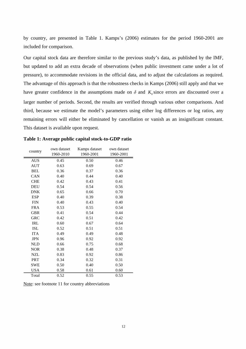
12

by country, are presented in Table 1. Kamps’s (2006) estimates for the period 1960-2001 are

included for comparison.

Our capital stock data are therefore similar to the previous study’s data, as published by the IMF,

but updated to add an extra decade of observations (when public investment came under a lot of

pressure), to accommodate revisions in the official data, and to adjust the calculations as required.

The advantage of this approach is that the robustness checks in Kamps (2006) still apply and that we

have greater confidence in the assumptions made on δ and 0K since errors are discounted over a

larger number of periods. Second, the results are verified through various other comparisons. And

third, because we estimate the model’s parameters using either log differences or log ratios, any

remaining errors will either be eliminated by cancellation or vanish as an insignificant constant.

This dataset is available upon request.

Table 1: Average public capital stock-to-GDP ratio

country own dataset 1960-2010

Kamps dataset 1960-2001

own dataset 1960-2001

AUS 0.45 0.50 0.46AUT 0.63 0.69 0.67BEL 0.36 0.37 0.36CAN 0.40 0.44 0.40CHE 0.42 0.43 0.41DEU 0.54 0.54 0.56DNK 0.65 0.66 0.70ESP 0.40 0.39 0.38FIN 0.40 0.43 0.40FRA 0.53 0.55 0.54GBR 0.41 0.54 0.44GRC 0.42 0.51 0.42IRL 0.60 0.67 0.64ISL 0.52 0.51 0.51ITA 0.49 0.49 0.48JPN 0.96 0.92 0.92NLD 0.66 0.75 0.68NOR 0.38 0.48 0.37NZL 0.83 0.92 0.86PRT 0.34 0.32 0.31SWE 0.50 0.40 0.50USA 0.58 0.61 0.60Total 0.52 0.55 0.53

Note: see footnote 11 for country abbreviations

13

4.3 Estimation results Since the seminal work of Aschauer (1989), the empirical literature on the quantitative effects of

public capital on output – under an aggregate production function approach12 – has grown in volume

and sophistication. In a meta analysis across a large set of empirical studies using industrial country-

data (both time series and panel) under the production function approach, Bom and Ligthart (2008)

conclude that estimates of the output elasticity of public capital range from -0.175 to 0.917.

However, several caveats, such as problems of data non-stationarity, endogeneity (potential

simultaneity and other forms of reverse causation) and heterogeneity for panel data analysis have

dominated much of this literature (see, among others, Romp and de Haan 2007 for a review).

Moreover, for the vast majority of these studies, the available time dimension of the data ends in

late ‘90s – early 2000.

The approach used in this paper is to conduct a large number of robustness checks to tackle some of

the main methodological problems of the earlier literature, in addition to employing an updated

dataset which spans until 2010. First, our empirical methodology is based on panel data, whose

increased dimension (N = 22; T = 50) enables us to increase the precision of our tests and

coefficient estimates. To deal with the problem of cross-sectional heterogeneity, first we apply the

analysis to 22 “old” OECD countries (advanced economies) and then restrict the sample according

to the degree of institutional, trade and monetary policy integration (that is, we also perform

estimates for the EU countries, and euro area countries only). Most importantly, we use specific

tests and empirical techniques to deal further with the problem of cross-sectional dependency. We

also tackle the problem of non-stationary data by estimating the production function relationship in

first differences, as well as ratios. Since most of the panel cointegration tests employed indicate the

absence of a cointegration relationship in levels, from a econometric point of view, our basic model

should rely on the first difference estimator. Finally, we deal with the problem of endogeneity and

reverse causation by using instrumental variables.

We therefore estimate the production function according to the three options proposed in section

4.1. In the absence of compelling evidence for panel cointegration, option 1) is estimated in first

differences to obtain stationary time series. In this respect, several tests have been employed, as

described below.

12 We focus on (and use in this paper) the production function approach, which is in line with our theoretical model. This is one - and arguably the most frequently employed - of three main approaches of the empirical literature on the marginal productivity of public capital. The other two are the cost function approach and the vector autoregressive (VAR) approach.

14

First, various panel as well as time series unit root tests generally indicate that our variables of

interest (all transformed in log terms) are non-stationary. In particular, the unit root test of Im,

Paseran and Shin (2003)13 fails to reject the null of unit root for all variables. Two other tests

employed, the Levin-Lin-Chu and Fisher tests, find a more mixed evidence: the null hypothesis that

all time series are non-stationary is rejected (at 10% significance level) for the income and private

capital stock variables. However, augmented Dickey-Fuller tests performed separately for each time

series in the panel also fail to reject the null of unit root. For more details and the panel tests results,

see Table A.1 in the Appendix 2.

Second, having failed to reject the null of unit root, the next step is to test for cointegration. To this

end, we employ the error-correction panel tests developed by Westerlund (2007),14 which

investigate the null hypothesis of no-cointegration by inferring whether the error-correction term in

a conditional panel model is equal to zero. For more details, see Persyn and Westerlund (2008). The

results – presented in Table A.2 in the Appendix 2 – indicate that the null fails to be rejected by

three tests, while only one rejects it at 5% significance level. Moreover, the alternative under the

latter test is that at least one cross-sectional unit displays cointegration, which is not very supportive

evidence either. Yet, given this result, for robustness purposes only, we also performed estimation

using panel cointegration techniques. We use various non-stationarity panel estimators,15 developed

by Pesaran, Shin and Smith (1999). Broadly confirming the results of the (three) cointegration tests,

the estimated models (available upon request) either do not imply convergence or the error

correction term is not statistically significant (although the value is in fact negative).

Third, for our regression equation in first differences, as well as for the options in ratios, we test for

cross-country dependency using the test proposed in Paseran (2004).16 The null of independency is

firmly rejected in all cases (see Table A.3 in the Appendix 2). Therefore, for Model 1 we use the

first difference estimator (thus also eliminating country fixed-effects), while for Models 2 and 3 we

use pooled OLS, in all three cases with Driscoll-Kraay standard errors. These standard errors are

robust to general forms of cross-sectional dependence in addition to temporal dependence (the error

13 Performed on demeaned data to render cross-sectionally independent disturbances. The test allows for heterogeneous short-run dynamics for different countries in the panel. 14 As implemented in Stata by Persyn and Westerlund (2008) 15As implemented in Blackburn and Frank (2007), namely: (i) a modified fixed-effects estimator; (ii) the mean-group estimator of Pesaran and Smith (1995), and (iii) the pooled mean-group estimator. The third estimator was also used in Calderon et al. (2011) for a panel of 88 industrial and developing countries over the period 1960-2000. First, the authors find evidence of cointegration in an infrastructure-augmented aggregate production function framework, in which aggregate output is produced using non-infrastructure physical capital, human capital, and infrastructure. Employing the pooled mean-group estimator, Calderon et al. find an output elasticity of infrastructure in the range of 0.07 to 0.10 16 As implemented in Stata based on Sarafidis and De Hoyos (2006).

15

structure is assumed to be heteroskedastic and autocorrelated up to the third lag and correlated

between the groups).

Fourth, we also test for the endogeneity of the public capital stock, but do not find strong evidence

for it in our sample (as explained in the data section, our private and public capital data are stocks –

and not investment flows – at the end of the previous year, while the labour input is the average

number of employees during the previous year). Using the Wu-Hausman F test and Durbin-Wu-

Hausman chi-sq test, we fail to reject the null of exogeneity across the three cross-sectional samples

at 5% significance level (for the EA-11 sample, the null is rejected only at 10%, but this seems to be

more an issue of the sample size). An instrumental variable-based estimation is nevertheless

performed as a robustness check, but the conclusions do not change. The estimation results and the

related tests are presented in Table A.4 of the Appendix 2.

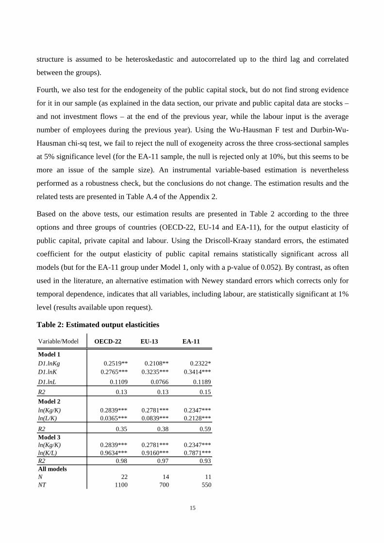
Based on the above tests, our estimation results are presented in Table 2 according to the three

options and three groups of countries (OECD-22, EU-14 and EA-11), for the output elasticity of

public capital, private capital and labour. Using the Driscoll-Kraay standard errors, the estimated

coefficient for the output elasticity of public capital remains statistically significant across all

models (but for the EA-11 group under Model 1, only with a p-value of 0.052). By contrast, as often

used in the literature, an alternative estimation with Newey standard errors which corrects only for

temporal dependence, indicates that all variables, including labour, are statistically significant at 1%

level (results available upon request).

Table 2: Estimated output elasticities

Variable/Model OECD-22 EU-13 EA-11

Model 1 D1.lnKg 0.2519** 0.2108** 0.2322*D1.lnK 0.2765*** 0.3235*** 0.3414***D1.lnL 0.1109 0.0766 0.1189R2 0.13 0.13 0.15Model 2ln(Kg/K) 0.2839*** 0.2781*** 0.2347***ln(L/K) 0.0365*** 0.0839*** 0.2128***

R2 0.35 0.38 0.59Model 3ln(Kg/K) 0.2839*** 0.2781*** 0.2347***ln(K/L) 0.9634*** 0.9160*** 0.7871***R2 0.98 0.97 0.93All modelsN 22 14 11NT 1100 700 550

16

Notes: The table shows the estimated coefficients and their significance level (*10%; **5%, ***1%). The three models correspond to the options proposed in section 4.1. Model 1 is in first differences (denoted by suffix D1.), models 2 and 3 in ratios. All variables are in natural logs (ln). The dependent variables are D1.lnY for Model 1; ln(Y/K) for Model 2 and ln(Y/L) for Model 3. Driscoll-Kraay standard errors are used throughout. The country groupings are explained in footnote 11.

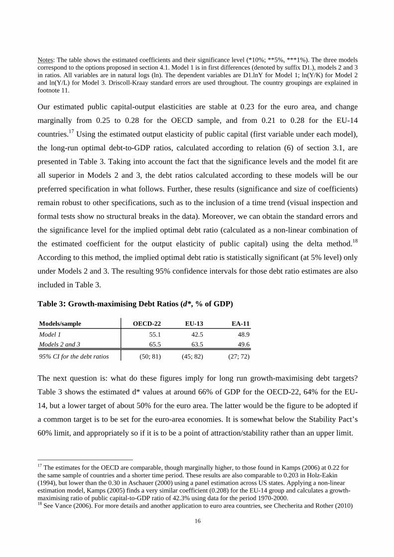
Our estimated public capital-output elasticities are stable at 0.23 for the euro area, and change

marginally from 0.25 to 0.28 for the OECD sample, and from 0.21 to 0.28 for the EU-14

countries.17 Using the estimated output elasticity of public capital (first variable under each model),

the long-run optimal debt-to-GDP ratios, calculated according to relation (6) of section 3.1, are

presented in Table 3. Taking into account the fact that the significance levels and the model fit are

all superior in Models 2 and 3, the debt ratios calculated according to these models will be our

preferred specification in what follows. Further, these results (significance and size of coefficients)

remain robust to other specifications, such as to the inclusion of a time trend (visual inspection and

formal tests show no structural breaks in the data). Moreover, we can obtain the standard errors and

the significance level for the implied optimal debt ratio (calculated as a non-linear combination of

the estimated coefficient for the output elasticity of public capital) using the delta method.18

According to this method, the implied optimal debt ratio is statistically significant (at 5% level) only

under Models 2 and 3. The resulting 95% confidence intervals for those debt ratio estimates are also

included in Table 3.

Table 3: Growth-maximising Debt Ratios (d*, % of GDP)

Models/sample OECD-22 EU-13 EA-11

Model 1 55.1 42.5 48.9Models 2 and 3 65.5 63.5 49.6

95% CI for the debt ratios (50; 81) (45; 82) (27; 72)

The next question is: what do these figures imply for long run growth-maximising debt targets?

Table 3 shows the estimated d* values at around 66% of GDP for the OECD-22, 64% for the EU-

14, but a lower target of about 50% for the euro area. The latter would be the figure to be adopted if

a common target is to be set for the euro-area economies. It is somewhat below the Stability Pact’s

60% limit, and appropriately so if it is to be a point of attraction/stability rather than an upper limit.

17 The estimates for the OECD are comparable, though marginally higher, to those found in Kamps (2006) at 0.22 for the same sample of countries and a shorter time period. These results are also comparable to 0.203 in Holz-Eakin (1994), but lower than the 0.30 in Aschauer (2000) using a panel estimation across US states. Applying a non-linear estimation model, Kamps (2005) finds a very similar coefficient (0.208) for the EU-14 group and calculates a growth-maximising ratio of public capital-to-GDP ratio of 42.3% using data for the period 1970-2000. 18 See Vance (2006). For more details and another application to euro area countries, see Checherita and Rother (2010)

17

The results presented above are subject to several estimation and inference uncertainties. First, data

related problems may preclude an exact estimation. Although taken from one source (OECD), and

building on the robustness checks performed in Kamps (2006), cross-checked with other data

sources (AMECO), the calculation of public investment series may still differ across countries.

Additionally, the delineation between private and public investment is sometimes blurred or inter-

sectoral reclassifications are possible at later stages (see for instance private-public partnership

projects).

Second, the assumption of our model is that debt is contracted only to finance productive

government expenditure and the accumulation of this expenditure is reflected in the public capital

stock, thereby reconstructed. While other government expenditure may also be productive, it is

difficult to disentangle their accumulation in a stock-approach of the production function. Moreover,

the effects may cancel out since not all capital expenditures are productive especially from a longer

term perspective.

Third, the estimated debt ratios are averages for the respective panel datasets and cannot be easily

generalised to a country level. In fact we were unable to obtain reasonable individual country results

for about half the cases. As other studies have found (Kamps, 2006; Stephan, 2000; Charlot and

Schmit, 1999), this was due to unreasonable variations in the estimates for α in some countries. This

appears to be the result of data misallocations in official sources, with too much public capital

spending classified as private in Germany, and too much private capital classified as public

elsewhere (the Netherlands), as Zagler and Durnecker (2003) point out. That puts reliable individual

country estimates beyond our reach primarily because of data limitations.

Our panel estimates can thus be used as a benchmark for a common debt policy. Moreover, using

panel estimation mitigates other econometric problems. As pointed out in Kamps (2006), the panel

analysis of the output returns to public capital, unlike individual country regressions, should not be

subject to multicollinearity problems as it exploits the cross-sectional variation in the data.

Furthermore, having a much larger number of observations (degrees of freedom) compared to

individual country regressions renders the estimators more efficient and the parameters of interest

can thus be estimated more precisely. Individual country estimates could be performed reliably only

on a much longer time series data, preferably at annual frequency (as quarterly data may prove

problematic in inducing too much noise), and potentially outside the production function

framework. Nonetheless, it is reassuring that our methods, despite all their potential uncertainties,

have produced a similar optimal debt estimate for the OECD area as Aiyagari and McGrattan (1998)

18

did (66% vs. 67% of GDP) using stylised numerical simulations of the welfare gains to holding debt

in the US (the dominant player in the OECD).

5. Debt targets in the setting of fiscal policy Having estimated optimal (growth-maximising) debt levels, how can we use this information to

guide fiscal policy? The identity which describes the evolution of an economy’s debt burden is:

( )d pdef r g d m (7)

where d represents the public debt-to-GDP ratio, d denotes the change in that ratio per unit of time,

pdef is the primary deficit (defined such that pdef > 0 implies a deficit), r is the average real rate of

interest charged on the debt burden, g is the rate of growth of output in real terms, and m is the

change in the ratio of the money stock to GDP per unit of time (de Grauwe, 2009).

If debt reduction programmes are not to result in inflation, the central bank must rule out undue

expansions of the money supply; that is, money may not grow faster than national output: 0m . In

that case, the debt ratio will stabilise ( 0d ) when:

( )pb r g d (8)

where pb is the budget’s primary surplus defined as ( ) /pdef G T Y pb (G is government

spending net of interest payments, and T are total government revenues). Thus, if r > g the

government must run a primary surplus to stop the debt burden rising and an even larger one to

reduce the debt burden. And that primary surplus will need to be bigger, the greater is r > g and the

greater is the initial value of d. Otherwise, the debt burden will rise.

But if r < g, the government may run a primary deficit as long as it is not larger than the term on the

right of (8). Thus the debt burden will shrink (without limit) so long as the primary surplus is always

set larger than the right hand side of (8).

Given that we have been able to define and estimate an optimal level of debt for the purposes of

maximising growth, the best strategy is to create a fiscal reaction function that sets the primary

surplus lower than the right hand side of (8) if current debt is below its optimal value (d < d*); but

above the right hand side of (8) if d > d*. In other words, the government is required to increase its

19

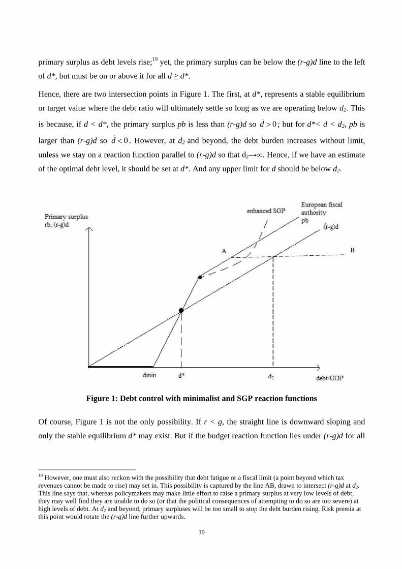
primary surplus as debt levels rise;19 yet, the primary surplus can be below the (r-g)d line to the left

of d*, but must be on or above it for all d ≥ d*.

Hence, there are two intersection points in Figure 1. The first, at d*, represents a stable equilibrium

or target value where the debt ratio will ultimately settle so long as we are operating below d2. This

is because, if d < d*, the primary surplus pb is less than (r-g)d so 0d ; but for d*< d < d2, pb is

larger than (r-g)d so 0d . However, at d2 and beyond, the debt burden increases without limit,

unless we stay on a reaction function parallel to (r-g)d so that d2→∞. Hence, if we have an estimate

of the optimal debt level, it should be set at d*. And any upper limit for d should be below d2.

Figure 1: Debt control with minimalist and SGP reaction functions

Of course, Figure 1 is not the only possibility. If r < g, the straight line is downward sloping and

only the stable equilibrium d* may exist. But if the budget reaction function lies under (r-g)d for all

19 However, one must also reckon with the possibility that debt fatigue or a fiscal limit (a point beyond which tax revenues cannot be made to rise) may set in. This possibility is captured by the line AB, drawn to intersect (r-g)d at d2. This line says that, whereas policymakers may make little effort to raise a primary surplus at very low levels of debt, they may well find they are unable to do so (or that the political consequences of attempting to do so are too severe) at high levels of debt. At d2 and beyond, primary surpluses will be too small to stop the debt burden rising. Risk premia at this point would rotate the (r-g)d line further upwards.

20

d, there is no zone of stability. In that situation, we would have to rely on debt restructuring plans to

reduce r and on structural reforms or competitiveness measures to raise g to support debt reduction.

Can we construct a fiscal reaction function to guarantee sustainability? One way is to require that,

for each percentage point that public debt increases above a certain threshold dmin, the primary

surplus pb must increase by at least (r-g+x)% points: where r is the average interest rate paid on

past debt, g is the average or potential growth rate, and x>0 is a margin dictated by the difference

d*-dmin. The value of x can be recovered once d* and dmin are known. Moreover, d2 would never be

reached since the debt burden will be falling for all d>d*. In other words, there would be no risk

premia and no d2. The value of x for this minimalist case would be:

min

*min)(

dd

dgrx

(9)

if dmin ≤ d ≤ d*+a; and zero otherwise. This is the budget rule any single European fiscal authority

would need to follow.

An alternative budget control rule is included in the new SGP (European Economy, 2011). Here

governments are required, under penalty of fines, to reduce their debt ratios each year by 1/20th of

the margin of their current debt over 60%. We could then take an optimal debt target of 50% from

Table 3 for the Euro area, treat the 60% limit as the start of the enforced debt reduction region, and

leave the 10% margin between them as a stability cushion. The slope of the reaction function above

d=60% would then be:

20

6.0d (10)

Because this slope is linear in d, this reaction function will be concave as drawn in figure 1. Such a

reaction function is increasingly aggressive at high debt levels, but milder just above 60%.

There are many other rules that satisfy (8) or, better, the condition necessary for debt to stabilise at

its target value. But there is a common element in all of them: to control a target variable such that it

eventually converges to a designated target, the policy instrument must follow a difference equation

of order at least as high as that governing the behaviour of the target – and one degree higher if full

convergence is to be feasible (Salmon 1982). The implication is that any implementable fiscal rule

with the property that it stabilises debt around its preferred target value must be constructed so that

21

the fiscal decisions are a function of the existing or projected debt level, an accumulation of past

deficits, and that it intersects the (r-g) line from below at d*.20

Four conclusions now follow: (i) to control the debt burden we need a sufficient primary surplus,

not a balanced budget rule; (ii) the control rule will be of sufficient order because it is of the same

order as its target variable (one degree higher if d is the currently projected debt level); (iii) it is

forward looking in that it anticipates the next value of debt and adjusts for that; and (iv) it stabilises

the debt at d* because it reaches (r-g)d from below or above d* (meaning that the difference

between d and d* is of the same order as d itself).

There is still the possibility that these rules break down through fiscal fatigue, because the economy

reaches the limit of its fiscal capacity, or because spending cuts depress tax revenues and output so

that debt ratios rise. The ultimate sanction (to prevent a reversion to AB in Figure 1), is to hand over

control of fiscal policy to a single European fiscal authority – as foreseen in the latest plans for the

euro area (European Council 2012) – to put us back on the original primary surplus line.

6. Concluding remarks and areas for further research

This paper makes several contributions. First, building on Aschauer (2000) the paper presents a

simple theoretical model and underlines the assumptions necessary to derive growth-maximising

public debt ratios. Second, on the basis of evidence on the productivity of public capital, we

estimate average growth-maximising public debt targets for three samples of OECD, EU and euro

area countries. To do so, we first reconstruct harmonised public and private capital stock series

across 22 OECD economies for the period 1960-2010, based on a previous study. Then, we estimate

the output productivity of public capital based on a production function approach and conduct a

large number of robustness checks to tackle some of the main methodological problems of the

earlier literature. Our estimates suggest that the euro area should target debt levels of around 50% of

GDP if member states are to have common targets. That is about 15 percentage points lower than

the growth-maximising debt ratio found for our OECD sample; and somewhat lower than the

Stability Pact’s debt ceiling of 60%. It therefore implies a comfortable safety cushion within which

debt ratios might be stabilised.

Overall, the paper provides the first theoretically-based estimates of the debt ratios that governments

should try to maintain if they wish to maximise growth. These are not arbitrary numbers, as many of

20 It is easy to construct such a rule if r<g. If it is not possible or politically acceptable to maintain such a rule when r>g, there is no fiscal space and no sustainable level of debt (because the economy lacks the fiscal capacity to sustain one).

22

the fiscal rules in the literature suggest, but are founded on long-run optimising behaviour, assuming

that governments implement the so-called golden rule over the cycle, that is, they contract debt only

to finance investment or, equivalently, finance current public spending only through current

revenues rather than borrowing.

Having defined or estimated optimal debt ratios for the purposes of maximising growth, different

fiscal rules that ensure these debt targets are achieved can be studied. We regard this as the most

important next step in this research. An overview of the properties such a rule would need to possess

was sketched in section 5. Given that fiscal deficits, and hence debt, are in part endogenous and

subject to random shocks - whether as a result of external shocks, policy errors or temporary

indiscipline - a fiscal control mechanism needs to define a “safe zone” around the preferred target

value, d*, within which the debt ratio can fluctuate freely; and specify a self-stabilising control

mechanism which ensures that the debt ratio will automatically return to its target value following a

shock. The implication of this safe zone is that governments that go beyond it, to higher levels of

debt, may have to be rescued. Lastly, there is the question of enforcement. Since the problem of

maintaining a safe level of debt can be reduced to one of sustaining a primary surplus budget rule,

this becomes a question of how to enforce such a rule. One has to recognise that such rules, however

well designed, may break down through insufficient fiscal capacity or because of the temptation for

self-interested time inconsistent behaviour (policy-makers backslide on their earlier commitments to

fiscal discipline). We leave this topic to further research too as it has more to do with appropriate

institutional design, monitoring, and punishment regimes, than with the rationale for, and best

design of, a debt targeting framework.

23

References Aiyagari, S. R. and E. R. McGrattan (1998), “The Optimal Quantity of Debt”, Journal of Monetary

Economics, 42, 447-69. Aizenman, J., K. Kletzer and B. Pinto (2007), “Economic Growth with Constraints on Tax Revenues

and Public Debt: Implications for Fiscal Policy and Cross-Country Differences”, NBER WP 12750, National Bureau of Economic Research, Cambridge MA.

Andersen, T., S. H. Jensen and L.H. Pedersen (2008), "The Welfare State and Strategies toward Fiscal Sustainability in Denmark", in R. Neck and J. Sturm (eds.), Sustainability of Public Debt, MIT Press.

Aschauer D. A. (1989), “Is Public Expenditure Productive?” Journal of Monetary Economics, 23, 177-200.

Aschauer D. A. (2000), “Do States Optimise? Public Capital and Economic Growth”, Annals of Regional Science, 34, 343-63.

Baum, A., C. Checherita-Westphal and P. Rother (2012), “Debt and growth: New Evidence for the Euro Area”, ECB Working Paper No. 1450, July, forthcoming in Journal of International Money and Finance.

Blackburne E.F. and M.W. Frank (2007), “Estimation of nonstationary heterogenous panels”, The Stata Journal, Vol. 7(2), 197-208.

Bokan, N., A. Hughes Hallett and S. E. H. Jensen (2012), “Fiscal Space and Optimal Debt Targets in a World of Ageing Populations”, forthcoming in Journal of International Money and Finance.

Bom, P.R.D. and J.E. Ligthart (2008), “How Productive is Public Capital? A meta-analysis.”, CESIfo Working Paper 2206, January.

Buti M, J. Nogueira Martins and A. Turrini (2007), “From Deficits to Debt and Back: Political Incentives under Numerical Fiscal Rules”, CESifo Economic Studies (2007) 53 (1): 115-152.

Calderón, C., E. Moral-Benito and L. Servén (2011), “Is Infrastructure Capital Productive? A Dynamic Heterogeneous Approach”, World Bank Policy Research Working Paper 5682, June.

Checherita, C. and P. Rother (2010), “The Impact of High and Growing Government Debt on Economic Growth: An Empirical Investigation in the Euro area”, ECB Working Paper 1237, August, published in European Economic Review 56 (2012), pp. 1392-1405.

Cecchetti, S. G., M. S. Mohanty and F. Zampolli (2011): "The Real Effects of Debt", BIS Working Papers No. 352.

Charlot S and B Schmitt (1999), "Public Infrastructure and Economic Growth in France's Regions" Paper presented to the 39th ERSA Congress, Dublin, Ireland.

Debrun X., L. Moulin, A. Turrini, J. Ayuso-i-Casals and M. S. Kumar (2008), "Tied to the mast? National fiscal rules in the European Union", Economic Policy, Vol. 23(4), 297-362.

De Grauwe, P. (2009), “Economics of Monetary Union”, Oxford University Press (8th edition), Oxford. Dixit, A.K. and L. Lambertini (2003): “Interactions of Commitment and Discretion in Monetary and

Fiscal Issues” American Economic Review, 93, 1522-42. European Council (2012), “Towards a Genuine Economic and Monetary Union”, European Council,

Brussels, 26 June 2012 (consilium.europa.eu/uedocs/cms_data/docs/pressdata/131201.pdf). European Economy (2011), “Public Finances in EMU – 2011”, European Economy, 3/2011.

DGII(EcFin), European Commission, Brussels, September. Ghosh, A. R., J. Kim, E. Mendoza, J.D. Ostry and M. Qureshi (2011), “Fiscal Fatigue, Fiscal Space

and Debt Sustainability in Advanced Economies”, WP 16782, NBER, Cambridge, MA.

24

Holz-Eakin D. (1994), “Public Sector Capital and the Productivity Puzzle”, Review of Economics and Statistics, 76, 12-21.

Hughes Hallett, A. (2008a), “Co-ordination without Explicit Co-operation: monetary-fiscal inter-actions in an era of demographic change”, European Economy: Economic Papers 305, European Commission, Brussels.

Hughes Hallett, A. (2008b), “Debt Targets and Fiscal Sustainability in an Era of Monetary Independence”, International Economics and Economic Policy, 5, 165-187.

Hughes Hallett, A. and D. Weymark (2007): “Fiscal Leadership and Central Bank Design”, Canadian Journal of Economics, 40, 607-27.

Hughes Hallett, A. and S.E.H. Jensen (2012) “Fiscal governance in the euro area: institutions vs. rules “Journal of European Public Policy, 19, 646-64.

Hughes Hallett, A., J. Lewis and R. Kattai (2012), “How Reliable are Cyclically Adjusted Budget Balances in Real Time?”, Contemporary Economic Policy, 30, 75-92.

Im, K.S., M.H. Pesaran, and Y. Shin (2003), “Testing for Unit Roots in Heterogenous Panels”, Journal of Econometrics, 115, 53–74.

Kamps, C. (2005), “Is There a Lack of Public Capital in the European Union”, European Investment Bank Economic Papers, 10, 72-93.

Kamps, C. (2006), “New Estimates of Government Net Capital Stocks for 22 OECD Countries, 1960-2001”, IMF Staff Papers, 53, 120-50. Koen, V. and P. Van den Noord (2006). “Fiscal gimmickries in Europe: One-off measures and

creative accounting”, in P. Wierts, S. Deroose, E. Flores and A. Turrini (eds.), Fiscal Policy Surveillance in Europe, Palgrave Macmillan, Basingstoke.

Libich, J. and P. Stehlik (2008), “Macroeconomic Games on Time Scales”, Dynamic Systems and Applications, 5, 274-78.

Libich, J., A. Hughes Hallett and P. Stehlik (2012), “Monetary and Fiscal Policy Interaction with Various Degrees of Commitment”, DP 6586, Centre for Economic Policy Research, London, paper presented to the American Economic Association meetings, Chicago, January.

Persyn D. and J. Westerlund (2008), "Error-correction–based cointegration tests for panel data," Stata Journal, vol. 8(2), 232-241.

Pesaran, H. (2004), “General diagnostic tests for cross section dependence in panels”, University of Cambridge, Faculty of Economics, Cambridge Working Papers in Economics No. 0435.

Pesaran, H., Y. Shin, and R. Smith (1999), “Pooled Mean Group Estimation of Dynamic Heterogeneous Panels”, Journal of the American Statistical Association, 94, 621-634.

Pesaran, H. and R. Smith (1995), “Estimating long-run Relationships from Dynamic Heterogeneous Panels”, Journal of Econometrics, 68, 79-113.

Reinhart, C. and K. Rogoff (2010), “Growth in a Time of Debt”, NBER Working Paper No. 15639. Romp, W. and J. de Haan (2005), “Public Capital and Economic Growth: A Critical Survey”, EIB

Papers, Vol. 10(1). Salmon, M. (1982), “Error Correction Mechanisms”, Economic Journal, 92, 615-29. Sarafidis, V., and R. E. De Hoyos (2006), “On testing for cross sectional dependence in panel data

models”, mimeo, University of Cambridge. Stephan A (2000), "Regional Infrastructure Policy and Its Impact on Productivity: a comparison of

Germany and France", Applied Economics Quarterly, 46, 327-56. Vance, C. (2006), “Marginal Effects and Significance Testing with Heckman’s Sample Selection

Model: A Methodological Note”, RWI Essen: Discussion Papers no. 39.

25

von Hagen, J. and G. Wolff (2006). “What do deficits tell us about debts? Empirical evidence on creative accounting with fiscal rules”, Journal of Banking and Finance, 30, 3259–79.

Westerlund, J. (2007), “Testing for error correction in panel data”, Oxford Bulletin of Economics and Statistics 69: 709–748.

Zagler, M. and G. Durnecker (2003), “Fiscal Policy and Growth”, Journal of Economic Surveys, 17, 397-418.

Appendix 1: Growth Maximising Levels of Public Capital and Debt

To derive the expressions for the optimal stock of public capital and debt, (3) and (4), we start from an infinitely lived representative agent with preferences over consumption, C, defined by the utility function:

1

0( 1) /(1 ) tV C e dt

(11)

where σ is the inverse of the elasticity of intertemporal substitution, and ρ is the agent’s rate of time preference. Output is given by (1), where there are constant returns to scale between private inputs as a group 1KL and the public (capital) input gK , and all variables have the interpretations given above. Employment may vary; but for simplicity there is no technical progress or depreciation.

Along the steady state growth path, public capital will grow at a constant rate, .g gK x K say, where x is the common growth rate of output, consumption and private capital. Government will have to levy a tax on output at a rate θ to pay interest on its debt and current expenditures. Public investment is financed by public debt. The government’s budget constraint is therefore:

. .gb r b K Y (12)

at interest rate r and debt level b. Private agents meanwhile maximise lifetime utility subject to their resource constraint (1 ) .K b C Y r b ; i.e. they maximise the current stage Hamiltonian

1 1 1[ 1] /(1 ) [(1 )( ) . ]gH C L K K r b C (13)

If employment levels are fixed, as in Aschauer (2000), we replace 1KL with K as the sole private input by normalising L to 1 and adjusting the units of (1-θ) by a factor of ( / )L K to reflect the contribution of labour to output at that assigned value.

But if employment levels are not fixed, we proceed in two steps. First we optimise (13) with respect to the private inputs 1KL as a whole, and also C and b.21 Then, eliminating L from (13) using the optimised function of K and gK just derived, we re-optimise a “concentrated” Hamiltonian to obtain optimal values for remaining private inputs, K and L, individually in the usual way. However, we do not need to use this second step in this paper. By contrast, first order conditions for the first step are:

21 Notice we do not optimize (13) with respect to Kg; (14) represents the private sector’s first order conditions given the government’s choice of Kg. This puts the government in a Stackelberg leadership position when it comes to choose Kg (in the form of ) conditional on the private sector reaction functions that emerge from (14), at equation (18) below.

26

(1 )(1 ) //

C

r

(14)

where 1/gK L K is the public to private inputs ratio. These conditions equate: the marginal utility of consumption to the shadow value of wealth, and the post-tax marginal product of private inputs, as well as the interest rate, to the rate of return on consumption. Together, they imply interest rates must equal the post-tax marginal product of the private inputs. Thus, from (14):

(1 )(1 )r (15)

It remains to determine an unconstrained optimal value for . Using (6) and the golden rule of deficit financing ,gK b the tax rate needed to service the debt in the long term is 1 .r That ensures sustainability. Substituting this expression into (9) yields

(1 ) /[1 (1 ) ]r (16)

which, given suitable transversality conditions, implies a steady state growth of consumption and output. Differentiating the top and using third expression in (8), this steady state growth rate is

1 1/ ( ) {(1 ) /(1 (1 ) ) }x C C r (17)

Now, maximising x with respect to yields the expression for the optimal value of given in

equation (3): 2(1 )

gK

K

= (18)

Notice that, using (1), we can also write

1

11 1 1 1[ ] [ ]

g g g

g

K K K

Y L K K L K

(19)

Replacing the optimal value of , we can calculate an optimal (growth-maximizing) long-run value for the debt-to-GDP ratio (see equation 4) as:

1*d =

1

2)1(

In other words, d* is the long-run optimal debt ratio for use when all inputs and input ratios take their optimised values. An alternative, short run expression for the cases when the capital ratio K/Y is fixed at its initial value is * ( / )d K Y if L is normalised at 1. In the more general version of the model, when L is not temporarily fixed or otherwise restricted, we get 1* ( / )d L K Y as the short run optimal debt ratio since, without normalisation, private sector inputs are 1KL rather than just K alone. This is the expression we might use to create a sequence of debt targets d* in transition from an excess debt position to long term optimal debt targets.

27

We can also derive a welfare maximising debt ratio, which emphasises consumption and is therefore a little smaller than the expression in (4). But we do not investigate that case in the paper.22

Appendix 2: Robustness and Diagnostic Tests

Table A.1: Panel Unit Root Tests

Test/Variables Test Statistic p-value Im-Pesaran-Shin test GDP -2.1 0.629 Public capital stock -1.6 0.999 Private capital stock -2.1 0.625 Labour -2.0 0.768 Levin-Lin-Chu test GDP -8.5 0.031 Public capital stock -6.4 0.496 Private capital stock -8.9 0.084 Labour -8.8 0.143 Fisher Test GDP 64.1 0.026 Public capital stock 147.4 0.270 Private capital stock 122.6 0.000 Labour 26.0 0.986

Note: The null hypothesis is a unit root (generally, all series are non-stationary). The deterministic components for all tests are a constant and trend; and the tests are augmented by 2 lags. The Im-Pesaran-Shin test is for cross-sectionally demeaned data. The Levin-Lin-Chu test is a pooled ADF test. Fisher test also uses an augmented (2-lags) Dickey-Fuller test. Tests performed for the full sample. Total number of observations is 1034. The panel dimensions are N,T = (22,50). Augmented Dickey-Fuller tests conducted on each time series in the panel (by country) also show fail to reject the null of non-stationarity for most countries.

Table A.2: Westerlund ECM panel cointegration tests

Test Statistic Value Z-value P-value Gt -3.102 -2.145 0.016 Ga -3.0 7.287 1.000 Pt -9.1 2.610 0.996 Pa -4.3 4.846 1.000

Note: The null hypothesis is no cointegration (Ho: the error correction parameter which determines the speed at which the system corrects back to the equilibrium after a sudden shock = 0). The four tests allow for a large degree of 22 To maximize welfare, in the sense of the current period’s consumption level (not growth rate), the government’s first order condition for maximizing H with respect to Kg must be added to (14) and all four first order conditions solved together. This is a Pareto optimal solution, and therefore welfare maximizing in that sense as well as consumption maximizing. But it lies at the extreme end of the contract curve between government and private sector because it ignores the government’s goal of maximizing steady state growth along side the short term consumption level. As such, it cannot be incentive compatible (if long term growth is a genuine objective); one player, the government, is made worse off even if the other, the private sector, is better off than in our solution. Hence, it cannot correspond to a cooperative bargain, Nash or otherwise. We do not pursue the more complicated stylized welfare gains approach of Aiyagari and McGrattan (1998) for the same reason.

28

heterogeneity both in the long-run cointegration relations and the short-run dynamics, as well as for dependence within and across countries. The first two tests investigate the null hypothesis of no-cointegration – as defined above - for all time series, against the alternative of at least one cross-sectional unit displaying cointegration. The other two tests pool information over all cross-sectional units to test the null of no-cointegration for all units, with a rejection of the null taken as rejection of cointegration for the panel as a whole. The tests are conducted on the whole sample. Similar results are obtained for the samples of EU-14 and EA-11.

Table A.3: Pesaran's test of cross sectional independence

Test Statistic Value P-value OECD-22 sample 40.313 0.000

EU-14 sample 31.603 0.000 EA-11 sample 25.745 0.000

Note: The null hypothesis is cross-sectional units are independent.

Table A.4: The Instrumental variable approach under Model 2

Variable/Model OECD-22 EU-14 EA-11

ln(Kg/K) 0.2613** 0.2501*** 0.2322*

ln(L/K) 0.0332*** 0.0801*** 0.3414***d* 58.1 54.5 48.9First stage statisticsPartial R2 0.9989 0.9988 0.9988N 990 630 495Underidentifiation test (Anderson LR stat); Ho = underidentified test (p-value) 6722.5 (0.000) 4244.6 (0.000) 3334.6 (0.000)Sargan statistic (overidentification test of all instruments); Ho = valid instrumentstest (p-value) 3.259 (0.5155) 7.889 (0.0957) 43.170 (0.000)Tests of endogeneity of the intrumented variable: ln(Kg/K)Wu-Hausman F test (H0: Regressor is exogenous)test (p-value) 0.6605 (0.4165) 0.6769 (0.4109) 3.7101 (0.0546)Durbin-Wu-Hausman chi-sq test (H0: Regressor is exogenous)test (p-value) 0.6628 (0.4156) 0.6806 (0.4093) 3.7123 (0.0540) Note: The estimator used is 2-stage least squares. The instrumented variable is ln(Kg/K) under preferred Model 2. Similar results are obtained under Model 3. Instruments are the first 5 lags of the variable. Using the first 3 lags or lags 3-5 instead does not change the results significantly. We take the value of the tests (especially the Sargan test) for the largest sample (the OECD-22) as relevant for the validity of the instruments.