fiscal redistribution around elections when democracy is
TRANSCRIPT

Fiscal redistribution around elections when democracyis not ‘‘the only game in town’’
Pantelis Kammas1• Vassilis Sarantides2
Received: 24 March 2016 /Accepted: 22 August 2016� The Author(s) 2016. This article is published with open access at Springerlink.com
Abstract This paper seeks to examine the implications of policy intervention around
elections on income inequality and fiscal redistribution. We first develop a simplified
theoretical framework that allows us to examine election-cycle fiscal redistribution pro-
grams in the presence of a revolutionary threat from some groups of agents, i.e., when
democracy is not ‘‘the only game in town’’. According to our theoretical analysis, when
democracy is not ‘‘the only game in town’’, incumbents implement redistributive policies
not only as a means of improving their reelection prospects, but also in order to signal that
‘‘democracy works’’, thereby preventing a reversion to an autocratic status quo ante at a
time of the current regime’s extreme vulnerability. Subsequently, focusing on 65 devel-
oped and developing countries over the 1975–2010 period, we report robust empirical
evidence of pre-electoral budgetary manipulation in new democracies. Consistent with our
theory, this finding is driven by political instability that induces incumbents to redistribute
income—through tax and spending policies—in a relatively broader coalition of voters
with the aim of consolidating the vulnerable newly established democratic regime.
Keywords Elections � New democracy � Redistribution � Income inequality
JEL Classification D63 � D72 � E62
Electronic supplementary material The online version of this article (doi:10.1007/s11127-016-0363-2)contains supplementary material, which is available to authorized users.
& Vassilis [email protected]
Pantelis [email protected]
1 Department of Economics, University of Ioannina, P.O. Box 1186, 45110 Ioannina, Greece
2 Department of Economics, University of Sheffield, 9 Mappin Str, Sheffield S1 4DT, UK
123
Public ChoiceDOI 10.1007/s11127-016-0363-2

1 Introduction
Numerous studies of political budget cycles (PBCs) suggest that close to the Election Day,
incumbents manipulate fiscal policy instruments in order to raise their reelection chances.1
A strand of this literature places the spotlight on factors conditioning the occurrence and
the strength of fiscal policy manipulation for electoral purposes (for a review of the
literature on conditional PBCs, see Klomp and de Haan 2013a). Starting from Schuknecht
(1996), the relevant literature suggests that fiscal manipulation is more likely in developing
countries, because institutional checks and balances are weaker, allowing for greater
political discretion over policy instruments.2 Shi and Svensson (2006) provide evidence of
electoral budget cycles in both developing and developed countries. However, they show
that the effect is far stronger in the former, where information asymmetries between voters
and politicians are more pronounced. Persson and Tabellini (2003, ch. 8) argue that
electoral cycles exist in developed economies as well. They find a strong budgetary rev-
enue cycle (government revenues as a percentage of GDP decline before elections) in
developed countries, though no evidence of electoral cycle in the overall budget balance.
Brender and Drazen (2005), on the other hand, argue that it is the age of the democratic
regime, and not a nation’s level of economic development, that matters for the observed
differences in electoral budget cycles. More precisely, they suggest that pre-electoral fiscal
manipulation is stronger in new democracies because of the voters’ lack of familiarity with
the electoral process.3 Following this rationale, Hanusch and Keefer (2014) suggest that
older political parties are able to address issues of credible commitment in a more effective
way, and therefore, fiscal manipulation for electoral purposes is more likely to occur in the
presence of younger political parties.
Another strand of the literature investigates how pre-electoral manipulation affects the
composition rather than the level of public spending and tax receipts. More precisely,
Schuknecht (2000) reports significant pre-electoral increases in public spending on
infrastructure for a sample of 24 developing countries. Several studies based on regional
data within countries have provided similar evidence (see, e.g., Khemani 2004; Drazen and
Eslava 2010). These findings are consistent with the theoretical model of Drazen and
Eslava (2010), according to which investment projects can be easily targeted to particular
geographical constituencies, increasing very effectively the political support received by
the incumbent. In contrast, Block (2002) and Vergne (2009) provide evidence that
politicians in developing countries shift the composition of spending towards current
expenditure and away from capital expenditure. Similar findings are obtained by Katsimi
and Sarantides (2012) for a sample of OECD countries. The implication of that study is
that policymakers seem to provide immediate benefit to voters by cutting current taxes,
whereas capital spending falls. The theoretical justification for these findings dates back to
1 The opportunistic approach was firstly formulated in the traditional model of ‘‘political business cycles’’by Nordhaus (1975). In contrast, the partisan approach deals with the behavior of ideologically motivatedpoliticians (see, e.g., Hibbs 1977).2 In support of this argument, Streb et al. (2009) show that electoral budget cycles are stronger in devel-oping countries than in industrial countries.3 More recently, Klomp and de Haan (2013b, c) provided evidence that the occurrence of a PBC is muchstronger in developing counties and ‘‘young democracies’’. However, Efthyvoulou (2012), using data for 27EU member states from 1997 to 2008, finds that incumbent governments tend to manipulate fiscal policy inorder to maximize their chances of being reelected. It is worth noting, though, that when Klomp and de Haan(2013d) employ a semi-pooled panel model to allow the impact of elections to vary across countries, theyfind no PBC in most countries.
Public Choice
123

Rogoff (1990). According to his argument, electorally motivated incumbents signal their
competence by shifting public policy towards visible budget items and away from capital
expenditures whose benefits can be discerned only in future periods.4
This paper contributes to the relevant literature in two ways. First, it seeks to investigate
the implications of pre-electoral manipulation of fiscal policy for income inequality. As
already mentioned, previous empirical studies have verified the presence of electoral cycles
in the size and the composition of public spending, as well as in the size and the com-
position of tax revenues (see, e.g., Persson and Tabellini 2003; Brender and Drazen, 2005;
Katsimi and Sarantides 2012). These fiscal policy changes are expected to have electorally
consequential distributional implications, which, to the best of our knowledge, have not
been examined in prior studies. To this end, we employ data from the Standardized World
Income Inequality Database (SWIID) in order to investigate the effect of electoral cycles
on (1) market income inequality (i.e., Gini coefficients before taxes and transfers); (2) net
income inequality (i.e., Gini coefficients after taxes and transfers); and (3) actual fiscal
redistribution (i.e., the percentage changes in Gini indices before and after transfers and
taxes).
Second, we extend the theoretical model of Aidt and Mooney (2014) in order to explore
the distributional implications of an election that takes place ‘‘in the shadow of revolu-
tion’’. The underlying feature of our model is that when the democratic regime is not fully
consolidated (i.e., in a new democracy), the incumbent faces a potential threat of revolution
from specific groups of agents, especially during pre-electoral periods (see, e.g., Fearon
2011; Little 2012; Little et al. 2015).5 As such, incumbent politicians in new democracies
collectively choose a pre-electoral fiscal policy taking into account the probability of a
democratic regime’s collapse in addition to their own reelection probability.6 In contrast, in
established democracies the incumbent cares only about the strategy that will maximize the
chances of remaining in office. This fundamental difference in the priorities of incumbents
in new and established democracies leads to a significant divergence in their optimal pre-
election strategies. More precisely, in stable democracies the incumbent allocates resources
to middle-income agents, in which the ‘‘pivotal’’ group of voters is located, with no effect
on actual fiscal redistribution. On the other hand, in new democracies incumbents also care
about the regime’s stability; they therefore target the benefits of fiscal policy to a broader
group of agents (which also includes low-income agents). The Gini coefficient, therefore,
is affected as income is transferred away from the ‘‘rich’’. Our theoretical results are in line
with the empirical findings reported by Brender and Drazen (2005). However, in our model
differences between new and old democracies are driven by the potential threat of
4 We have to note that manipulation of the composition of fiscal policy seems particularly relevant indeveloped economies in which the incumbent may avoid deficit creation owing to the fear of voters’disfavor (see, e.g., Brender and Drazen 2008).5 It is frequently argued in the literature that only antidemocratic elites (e.g., military juntas and oligarchs)can pose serious threats in a newly established democracy (see Acemoglu and Robinson 2006). Nonetheless,empirical and anecdotal evidence strongly suggests that the support of the citizenry for the institutions ofdemocracy cannot be taken for granted (see Linz and Stepan 1996). For instance, a few years after Brazil’sdemocratization, according to a Brazilian national survey published in February 1992, the poorest citizenswere the least supportive of democracy.6 The tension that surrounds pre-election campaigns in a newly established democratic regime is animportant factor that contributes significantly to political instability. In many cases, it has been observed thatperiods around Election Day are the times of greatest vulnerability for democratic regimes (e.g., Bolivia1978–1980; Nigeria 1993 and Pakistan 1977). Brender and Drazen (2007) provide empirical evidence that in‘‘young democracies’’ the regime is almost three times more likely to collapse in election years than in non-election years.
Public Choice
123

revolution and not by the electorate’s lack of familiarity with the democratic process. Our
intuition is closer to Brender and Drazen (2007), who suggested that the attitude of the
citizenry towards democracy is important in preventing democratic collapse, and fiscal
manipulation can act as an instrument to convince them that ‘‘democracy works’’.
Our paper could also be related to a parallel literature that highlights the threat of
revolution as a key ingredient in democratic transitions (see, e.g., Acemoglu and Robinson
2000, 2006; Przeworski 2009; Aidt and Jensen 2014). Starting from Tullock (1974), a large
number of studies highlight that in many historical cases elites offered voting rights to
poorer segments of the society in order to avoid revolutions. This is because extension of
the voting franchise acts as a commitment mechanism for future fiscal redistribution from
the elites (i.e., the rich) to the poor. This commitment can mitigate the threat of a ‘‘crude
redistribution’’ that would result from a successful revolution fomented by the low-income
agents.
All of these studies recognize the importance of the so-called de facto political power
and consequently of the threat of revolution as a catalyst for democratic transitions.7
However, they assume that de facto political power disappears just after the transition to a
democratic regime and, therefore, it does not affect the implemented economic policy in
democracies. Building on this rationale, the present paper suggests that de facto political
power and the consequent threat of revolution can affect implemented economic policies
even in democracies, especially during the first years of the transition. This is because in
new democracies that are not fully consolidated, citizens face an option to revolt against
the incumbent government if the latter fails to demonstrate a minimum level of compe-
tence. To this end, incumbents may opt for implementing pro-poor economic policies in
order to convince the low-income agents that ‘‘democracy works’’, mitigating the risk of
revolution that can lead to a democratic regime’s collapse.8
To test the theoretical predictions of the model, we focus our attention on a dataset of 65
developed and developing countries over the 1975–2010 period. Our analysis indicates that
in new democracies elections exert a positive and significant impact on actual fiscal
redistribution. Subsequently, we attempt to further corroborate our theoretical prediction
that political instability is the driving force of our results. We measure instability using
cross-country data on state repression and state violence. Our findings suggest that the
effect of elections is stronger when new democracies are characterized by more political
instability, especially when the latter is proxied by state violence. Consistent with the
model, in vulnerable democratic regimes incumbent politicians allocate resources—
through tax and spending polices—towards the poorer segments of society in order to
convince them that ‘‘democracy works’’, mitigating the risk of a potential revolution.
The rest of the paper is organized as follows. Section 2 presents the theoretical analysis
and deduces key implications. Section 3 describes the data and the empirical setup,
whereas Sect. 4 presents the empirical results. Finally, Sect. 5 summarizes the main
findings.
7 We define de facto political power as the ability of a group of individuals to solve collective actionproblems (Olson 1965) and to be organized to protest or to revolt in order to impose their wishes on society.For more details on this, see, e.g., Acemoglu et al. (2005).8 Linz and Stepan (1996), summarizing the experience of the new democracies in southern Europe, suggestthat the consolidation of democracy takes place only when ordinary citizens come to believe that democracyis superior to any other form of governance. Before that point, their pro-democratic feelings cannot be takenfor granted.
Public Choice
123

2 Theoretical framework
This section develops a simple theoretical model that borrows its main features from
Lohmann (1998) and Aidt and Mooney (2014). Our theoretical framework allows us to
compare the distributional implications of pre-electoral fiscal policies between new and
established democracies.
We consider an economy populated by three types of individuals: rich (R) of size dR,middle-income (M) of size dM, and poor (P) of size dP, in which we assume that dM[dR ? dP and dR ? dM ? dP = 1. The rich, the middle-income group, and the poor have
fixed incomes yR, yM, and yP, respectively, during periods t = 1, 2, where in addition we
assume that yR[ yM[ yP. The tax rate (s) is proportional to the income of each group, and
it is fixed at a level of s ¼ �s in both periods. The elected national government in each
period collects tax revenues and runs a balanced budget. Moreover, it decides whether to
use the given tax revenues in order to finance a lump-sum targeted transfer to the low-
income group (TPt ), or, alternatively to the middle-income group (TM
t ), or, finally, to the
rich agents (TRt ). The government decides also whether to extract resources from public
funds by diverting tax revenues to private rents (rt) for itself. Therefore, the government’s
budget constraint is dPTPt þ dMTM
t þ dRTRt þ rt ¼ �s�y, where �y is the average income. An
election takes place between the two periods.
Citizens’ well-being depends on three factors: (1) the budget allocation, (2) the quality
of the politician running the government, and (3) random events (bad or good luck). The
utility generated by the budget allocation and private consumption is as follows:
uPt ¼ ð1� �sÞyP þ TPt ; ð1Þ
uMt ¼ ð1� �sÞyM þ TMt ; ð2Þ
uRt ¼ ð1� �sÞyR þ TRt : ð3Þ
The quality of governance matters to the citizens because the utility they get from a
given budget allocation increases with the quality of the incumbent politician. The total
utility of each type of agent is, respectively, as follows:
UPt ¼ ð1� �sÞyP þ TP
t þ qt þ lt; ð4Þ
UMt ¼ ð1� �sÞyM þ TM
t þ qt þ lt; ð5Þ
URt ¼ ð1� �sÞyR þ TR
t þ qt þ lt; ð6Þ
where qt is a quality shock, which determines how competent the incumbent is, and lt is a‘‘luck’’ shock that makes the incumbent look more or less competent than may be the case.
The fundamental information assumption of the model is that the voters observe total
utility, but they are unable to decompose this between lump sum transfers, the quality
shock (qt) and the ‘‘luck’’ shock (lt).9 Although the two shocks are unobserved, they are
both drawn from known distributions. The luck shock (lt) is drawn independently in each
9 The underlying assumption is that voters are ill informed about the finer details of public finance. This isanalogous to the assumption in Lohmann (1998) that voters do not observe the implemented monetarypolicy directly.
Public Choice
123

period and is equal to ±1/2, each occurring with probability p ¼ 1=2.10 The quality shock
(qt) is a characteristic of the politician and follows a uniform distribution over � 12; 12
� �. If
the politician is reelected, the quality shock from period 1 also applies to period 2, whereas
if a new politician is elected in period 2 a new quality shock is drawn from the above-
mentioned known uniform distribution.
The total utility of the incumbent is increasing and quasi-concave. For algebraic sim-
plicity, we use an additively separable function of the form:
W ¼ lnðr1Þ þ pIb lnðE þ r2Þ; ð7Þ
where 0\b\1 is a discount factor and pI is the probability that the incumbent is reelected.
The quantity rt denotes rents grabbed in period t = 1, 2, and E denotes the exogenous rents
from winning the election.11
We solve the model under two alternative political regimes. The first one (that will
serve as benchmark) is an established democratic regime in which democracy is ‘‘the only
game in town’’. The second political regime is a newly established democracy wherein the
incumbent faces a potential threat of revolution from some groups of agents.
2.1 Fiscal redistribution when democracy is ‘‘the only game in town’’
First, consider the benchmark case of an established democracy. The timing of the events
in this case is as follows: (1) At the beginning of period 1, a balanced budget
TP1 ; T
M1 ; TR
1 ; r1� �
is implemented, and (2) the two random shocks q1 and l1 are realized.
Random shocks are not observed directly by anyone, but all agents are able to observe total
utility. (3) At the end of the first period, elections take place, and the voters either reelect
the incumbent politician or elect a new politician. (4) The winner implements a balanced
budget TP1 ; T
M1 ; TR
1 ; r1� �
in period 2. (5) A new luck shock l2 is realized. If the incumbent
of the first period is reelected the quality shock from period 1 (i.e.,q1) carries over to period
2. Otherwise, a new quality shock q2 is realized. (6) Finally, the total utility is determined
and observed by all agents.
Solving the model by backward induction, we see that, in period 2, the politician has no
incentive to behave well and therefore, appropriates the maximum amount of rents r�2 ¼ �s�y,implying zero targeted transfers to all groups of agents: TP�
2 ¼ TM�2 ¼ TR�
2 ¼ 0. Equa-
tions (4), (5), and (6) imply that voters are clearly better off with a more competent (high
q) politician, as this gives them more utility in period 2. Thus, they use elections as a mean
of reappointing competent politicians and ousting incompetent ones, taking into account
their observed utility in period 1 and knowing that the opponents’ expected quality on
Election Day is EðqÞ ¼ 0.12 We now describe how this takes place and how it shapes
politicians’ incentives in period 1.
10 That is, the luck shock (lt) follows a Bernoulli distribution with p(-1/2) = p(1/2) = 1/2.11 These exogenous ego-rents (E) reflect the value attached to winning the elections and holding office (seePersson and Tabellini 2000, ch. 3.2, for more details on this).12 This is because the quality shock of the opponent is drawn from a uniform distribution that is known tothe voters.
Public Choice
123

2.1.1 The optimal voting behavior and the utility targets
In order to describe how the politicians’ decisions in period 1 affect the probability of
reelection, we need to describe optimal voting behavior. In period 2, since r�2 ¼ �s�y and
TP�2 ¼ TM�
2 ¼ TR�2 ¼ 0, the welfare of agents in the three groups is as follows:
UP2 ¼ ð1� �sÞyP þ q02 þ l2; ð8Þ
UM2 ¼ ð1� �sÞyM þ q02 þ l2; ð9Þ
UR2 ¼ ð1� �sÞyR þ q02 þ l2; ð10Þ
where q02 ¼ pIq1 þ ð1� pIÞq2. This is because, if the incumbent of the first period gets
reelected the quality shock from period 1 (q1) carries over to period 2, whereas if a new
politician is elected a new quality shock (q2) is realized. Since all politicians implement the
same post-election budget, the only reason voters care about who gets reelected is that
politicians’ qualities vary. As seen from period 1, the expected quality of the politician
elected in period 2 is:
E1q02 ¼ pIE1q1 þ ð1� pIÞE1ðE2q2Þ ¼ pIE1q1: ð11Þ
This expression follows because the expected quality of a new politician is zero on
average, i.e., E1ðE2q2Þ ¼ E2q2 ¼ 0. Thus, the voters want to reelect the incumbent if and
only if their estimate of the politician’s quality at the end of period 1 is positive, that is, if
and only if E1q1 [ 0. Since in our model dM[ dR ? dP, the pivotal group of voters is the
group of the middle class (M). Thus, we further proceed by examining how the preferences
of this specific group shape the actions of the politician.
More precisely, to form a Bayesian estimate of the expected quality of the incumbent,
the middle-income voters use information on the observed utility of the first period UM1 and
their knowledge about the incumbent’s equilibrium budget strategy. The equilibrium
budget strategy of the incumbent is ~uM1 ¼ ð1� �sÞyM þ ~TM1 . Subtracting the equilibrium
budget strategy (~uM1 ) from Eq. (5), we get:
UM1 � ~uM1 ¼ TM
1 � ~TM1 þ q1 þ l1 ¼ q1 þ l1: ð12Þ
The last equality makes use of the fact that in equilibrium, TM1 ¼ ~TM
1 . Equation (12)
shows that voters can infer the sum of the two shocks using their knowledge of the
equilibrium. However, they are unable to decompose those two shocks and, therefore, to
infer the quality of the politician. A rational voter can solve the resulting signal extraction
problem and estimate that:
E1q1 ¼r2q
r2l þ r2qðUM
1 � ~uM1 Þ ¼1
4ðUM
1 � ~uM1 Þ: ð13Þ
Based on Eq. (13), we conclude that the incumbent politician will be reelected if the realized
utility of the middle-income agents exceeds the budget-related utility that the voters expect the
incumbent to deliver in equilibrium, that is, if and only ifUM1 � ~uM1 [ 0. Using Eq. (12), we can
restate this criterion as q1 þ l1 [ ~TM1 � TM
1 . Having assumed that l1 follows a Bernoulli
distribution with P(-1/2) = P(1/2) = 1/2 and that q1 follows a uniform distribution over
� 12; 12
� �, we get that the summation of q1 ? l1 follows a uniform distribution over ½�1; 1�.
Consequently, the probability of reelection as perceived by the incumbent is
Public Choice
123

pI ¼ Pðq1 þ l1 [ ~TM1 � TM
1 Þ ¼ 1
2½1þ ðTM
1 � ~TM1 Þ�: ð14Þ
Equation (14) shows that the reelection probability is increasing in budgetary transfers
directed to the middle class. Therefore, the incumbent has an incentive to select the
allocation of tax revenues so as to increase redistribution towards this specific group of
individuals.
2.1.2 The budget allocation in equilibrium
Combining Eqs. (7) and (14) with the government’s budget constraint, we conclude that
the equilibrium values for TP1 ; T
M1 ; TR
1 ; r1� �
are those that maximize incumbent’s inter-
temporal utility:
W ¼ lnðr1Þ þ1
2½1þ ðTM
1 � ~TM1 Þ�
� �b lnðE þ r2Þ; ð15Þ
subject to the first period’s budget constraint dPTP1 þ dMTM
1 þ dRTR1 þ r1 ¼ �s�y and the rent
extraction decision of the second period (i.e., r�2 ¼ �s�y). Then, Appendix 1-Supplementary
material shows:
Proposition 1 The incumbent generates a rational political budget cycle. The post-election
result is TP�2 ¼ TM�
2 ¼ TR�2 ¼ 0 and r�2 ¼ �s�y. The pre-election result is r�1 ¼ �s�y� dMTM�
1
(which is smaller than r�2 for TM�1 [ 0) and TM�
1 ¼ �s�yb lnðEþr�2Þ�2dM
dMb lnðEþr�2Þ (which is positive if
�s�yb lnðE þ r�2Þ[ 2dM). Finally, TP�1 ¼ TR�
1 ¼ 0.
Thus, during the pre-electoral period the incumbent has an incentive to reduce extracted
rents and correspondingly to increase the transfers to the middle-income voters in order to
convince them of their quality and thereby remain in office for a second period. However,
since pre-electoral transfers are directed exclusively to the middle-income group and not to
the low-income group of agents, elections fail to reduce after-taxes-and-transfers income
inequality and consequently to increase the actual amount of redistribution.13
Corollary 1 Since pre-election transfers are strictly targeted to the middle-income group
they do not reduce the after-taxes-and-transfers Gini coefficient.
2.2 Fiscal redistribution when the election takes place in the shadowof revolution
In this section, we solve the model for the case of a newly established democracy. More
precisely, we assume that during the first years of a political transition, wherein democracy
is not ‘‘the only game in town’’, citizens have an option to revolt against the incumbent if
the latter fails to ensure a minimum amount of competence. In this case, the survival of the
democratic regime cannot be taken as given, since there is a probability of collapse and a
consequent reversal to other forms of governance.14
13 We note that the tax rate (s) is proportional to the income of each group, and it remains fixed at a level ofs ¼ �s in both periods.14 Previous studies (e.g., Acemoglu and Robinson 2000, 2006; Aidt and Jensen 2014) suggest that threat ofrevolution is an important factor for democratization, but it disappears when the regime becomes demo-cratic. Building on this rationale, our model investigates whether the threat of revolution may affect theimplemented economic policy in democratic regimes, especially during the first years of the transition.
Public Choice
123

The timing of the events in this case is as follows: (1) At the beginning of period 1, a
balanced budget TP1 ; T
M1 ; TR
1 ; r1� �
is implemented. (2) The two random shocks q1 and l1 arerealized. As before, the random shocks are not observed directly by anyone, but all agents are
able to observe total utility. (3) At the end of the first period, elections take place, and the
voters either reelect the incumbent politician or elect a new one. (4) After elections, the
citizens decide whether to revolt or not. More precisely, if the incumbent politician fails to
convince the citizens that his quality exceeds aminimum amount of competence, a revolution
takes place and the democratic regime collapses with probability pR. (5) In period 2,
regardless of whether the democratic regime survived or not (in stage 4), the official
implements a balanced budget TP2 ; T
M2 ; TR
2 ; r2� �
. (6) A new luck shock l2 is realized. If thedemocratic regime has survived and the incumbent of the first period is reelected, the quality
shock from period 1 (i.e., q1) carries over to period 2. Otherwise, a new quality shock q2 is
realized. (7) Finally, total utility is determined and observed by all agents.
Again, solving the model by backward induction, we see that in period 2 the official
(whether democratically elected or not) has no incentive to behave well. Therefore, he
extracts the maximum amount of rents r�2 ¼ �s�y, implying zero targeted transfers to all
groups of agents: TP�2 ¼ TM�
2 ¼ TR�2 ¼ 0. As in Sect. 2.1, Eqs. (4), (5), and (6) imply that
citizens are clearly better off with a more competent (high q) politician, as this increases
their utility in period 2. Thus, they use elections as a mean of reappointing a competent
politician and throwing the incompetent ones out of office. However, in the case of a new
democracy, the citizens have one additional option in order to ensure a minimum amount
of competence (i.e., quality that equals to �q), which is to revolt and oust the incumbent
from office. We now describe how this takes place and how it shapes politicians’ incentives
in period 1.
2.2.1 The optimal voting behavior and the utility targets
Since dM[ dR ? dP, when elections take place, the pivotal group of voters remains the
middle-income group (M). Following the rationale developed in Sect. 2.1.1, the criterion
under which the middle class votes for the incumbent is UM1 � ~uM1 [ 0, which generates the
following probability of reelection as perceived by the incumbent: pI ¼ 12½1þ ðTM
1 � ~TM1 Þ�.
Therefore, the reelection probability in new and established democracies is identical, and it
increases by the amount of transfers (TM1 ) directed to the middle-income group.
2.2.2 The threat of revolution
Following the rationale of the relevant theoretical literature, we assume that in newly
established democracies’ elections also act as a public signal of government’s popularity.
This helps the citizens to solve potential problems of collective action and to revolt against
the incumbent whenever a high level of anti-regime sentiments emerges (see, e.g., Fearon
2011; Little 2012; Little et al. 2015). Therefore, we assume that at the end of the first
period (after elections are held), the citizens from the middle-income (M) and the low-
income (P) groups decide whether to revolt or not.15 More precisely, citizens revolt
15 Several studies suggest that the consolidation of democracy takes place only when ordinary citizens cometo believe that democracy is superior to any other form of governance (see, e.g., Linz and Stepan 1996;Brender and Drazen 2007). Before that point, the pro-democratic feelings of the masses cannot be taken forgranted.
Public Choice
123

whenever they estimate that the quality of the incumbent at the end of the first period is
negative and below a threshold quality level �q. That is, if and only if E1q1\�q\0. This
condition is binding only in the case of the low-income citizens. That is because middle-
income citizens determine the probability of reelection by their votes and, therefore, they
demand even higher (i.e., a positive) competence at the end of the first period in order to
reelect the incumbent.16 Thus, we focus on the low-income group of agents and examine
how the threat of potential revolution shapes a politician’s incentives in period 1.
As in Sect. 2.1.1, in order to form a Bayesian estimate of the expected quality, citizens
rely on the observed utility of the first period UP1 and their knowledge about the incum-
bent’s equilibrium budget strategy. The equilibrium budget strategy of the incumbent is
~uP1 ¼ ð1� �sÞyM þ ~TP1 . Subtracting equilibrium budget strategy (~uP1 ) from Eq. (4) we get:
UP1 � ~uP1 ¼ TP
1 � ~TP1 þ q1 þ l1 ¼ q1 þ l1: ð16Þ
Equation (16) shows that voters can infer the sum of the two shocks using their
knowledge of the equilibrium. However, they are unable to decompose them and, there-
fore, to infer the quality of the politician. A rational citizen can solve the resulting signal
extraction problem and estimate that:
E1q1 ¼r2q
r2l þ r2qðUP
1 � ~uP1 Þ ¼1
4ðUP
1 � ~uP1 Þ: ð17Þ
Based on Eq. (17), we conclude that low-income citizens will decide to revolt if14ðUP
1 � ~uP1 Þ\�q. Using Eq. (16), we can restate this criterion as: q1 þ l1\ ~TP1 � TP
1 þ 4�q,
where q1 ? l1 follows a uniform distribution over ½�1; 1�. Consequently, we get the
following probability of revolution as perceived by the incumbent:
pR ¼ Pðq1 þ l1\ ~TP1 � TP
1 þ 4�qÞ ¼ 1
2½1þ ð~TP
1 � TP1 Þ þ 4�q�: ð18Þ
Assuming that whenever a revolution takes place it is successful and the democratic
regime collapses, we derive the following probability of democratic regime survival:
pD ¼ 1� pR ¼ 1
2½1þ ðTP
1 � ~TP1 Þ � 4�q�: ð19Þ
Equation (19) shows that the probability of a democratic regime’s survival is increasing in
income transfers to the low-income group of individuals (TP1 ). Thus, when ‘‘elections take
place in the shadow of revolution’’, the incumbent has an incentive to increase redistribution
towards the poorer agents. This strategy allows the incumbent to stabilize the political regime
and consequently to increase the probability of remaining in office. In other words, in a
relatively new democracy, focusing solely on the preferences of the middle-income group is
not a sufficient condition for continuing in office, since the incumbent also faces a potential
threat of revolution from the low-income group. Therefore, the total utility of the incumbent
in the case of a new democracy takes the following form:
W ¼ lnðr1Þ þ pDpIb lnðE þ r2Þ; ð20Þ
where pI is the probability of the incumbent being re-elected and pD is the probability of
the democratic regime surviving.
16 As in Sect. 2.1, middle class citizens vote for the incumbent only if their estimate of his or her quality atthe end of the first period is positive (i.e., if E1q1[ 0).
Public Choice
123
2.2.3 The budget allocation in equilibrium
Combining Eqs. (14), (19), and (20) with the government’s budget constraint, we conclude
that the equilibrium values for TP1 ; T
M1 ; TR
1 ; r1� �
are those that maximize the incumbent
inter-temporal utility in the case of a newly established democracy:
W ¼ lnðr1Þ þ1
2½1þ ðTP
1 � ~TP1 Þ � 4�q�
� �1
2½1þ ðTM
1 � ~TM1 Þ�
� �b lnðE þ r2Þ; ð21Þ
subject to the first period’s budget constraint, dPTP1 þ dMTM
1 þ dRTR1 þ r1 ¼ �s�y, and the
rent extraction decision of the second period (i.e., r�2 ¼ �s�y). Equation (21) shows that in a
new democracy the incumbent should accommodate the needs of the low and middle-
income groups (TP1 andT
M1 Þ in order to maximize its probability of remaining in office. This
is because transfers directed to the low-income group of agents (TP1 ) serve as a policy
instrument of democratic consolidation, whereas transfers directed to the middle-income
group (TM1 ) represent a policy instrument that affects the reelection probability when
elections are held. Then, Appendix 1-Supplementary material shows:
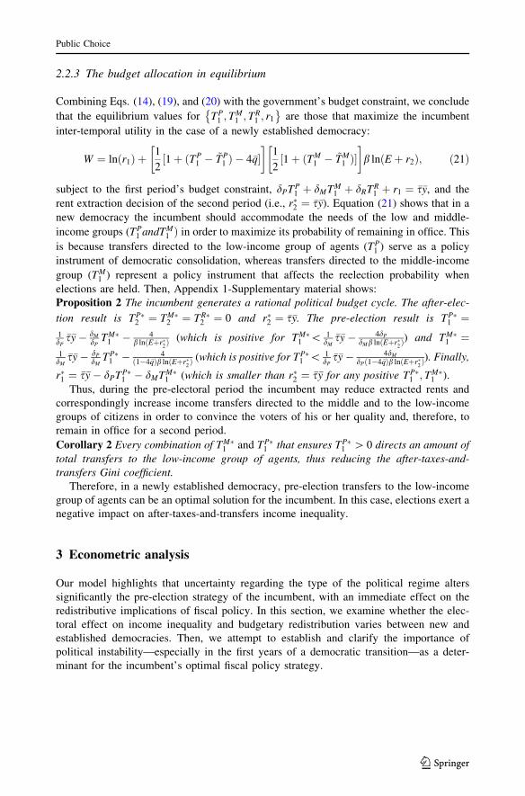
Proposition 2 The incumbent generates a rational political budget cycle. The after-elec-
tion result is TP�2 ¼ TM�
2 ¼ TR�2 ¼ 0 and r�2 ¼ �s�y. The pre-election result is TP�
1 ¼1dP�s�y� dM
dPTM�1 � 4
b lnðEþr�2Þ (which is positive for TM�
1 \ 1dM
�s�y� 4dPdMb lnðEþr�
2Þ) and TM�
1 ¼1dM
�s�y� dPdM
TP�1 � 4
ð1�4�qÞb lnðEþr�2Þ (which is positive for T
P�1 \ 1
dP�s�y� 4dM
dPð1�4�qÞb lnðEþr�2Þ). Finally,
r�1 ¼ �s�y� dPTP�1 � dMTM�
1 (which is smaller than r�2 ¼ �s�y for any positive TP�1 ; TM�
1 ).
Thus, during the pre-electoral period the incumbent may reduce extracted rents and
correspondingly increase income transfers directed to the middle and to the low-income
groups of citizens in order to convince the voters of his or her quality and, therefore, to
remain in office for a second period.
Corollary 2 Every combination of TM�1 and TP�
1 that ensures TP�1 [ 0 directs an amount of
total transfers to the low-income group of agents, thus reducing the after-taxes-and-
transfers Gini coefficient.
Therefore, in a newly established democracy, pre-election transfers to the low-income
group of agents can be an optimal solution for the incumbent. In this case, elections exert a
negative impact on after-taxes-and-transfers income inequality.
3 Econometric analysis
Our model highlights that uncertainty regarding the type of the political regime alters
significantly the pre-election strategy of the incumbent, with an immediate effect on the
redistributive implications of fiscal policy. In this section, we examine whether the elec-
toral effect on income inequality and budgetary redistribution varies between new and
established democracies. Then, we attempt to establish and clarify the importance of
political instability—especially in the first years of a democratic transition—as a deter-
minant for the incumbent’s optimal fiscal policy strategy.
Public Choice
123

3.1 Dataset and variables
Following previous studies, we measure income inequality by the Gini coefficient (index)
of income distribution. The Gini coefficient ranges from a minimum value of zero, when
the incomes of all individuals are the same, to a maximum of one in a population when all
the wealth is concentrated in a single individual. However, a primary concern when
employing income inequality estimates in cross-country empirical research is data com-
parability, both over time and across countries. For this reason, our preferred data are
obtained by the Standardized World Income Inequality Database (SWIID), developed by
Frederick Solt (2009). The SWIID maximizes the comparability of income inequality
statistics for the largest possible sample of countries and years, namely, for 174 countries
for as many years as possible from 1960 to 2010. For the construction of the dataset, Solt
(2009) employed a customized missing-data algorithm to standardize Gini estimates from
all major existing resources of income inequality data (e.g., Luxembourg Income Study,
World Income Inequality Database). An important advantage of the SWIID is that it
provides Gini estimates before taxes and transfers (market income), as well as after-taxes-
and-transfers (net income). They are denoted as gini_market and gini_net, respectively.
Furthermore, the percentage change between gini_market and gini_net gives us an estimate
of fiscal redistribution17:
redistit ¼gini marketit � gini netit
gini marketit� 100 ð22Þ
This decomposition of income inequality, before and after-taxes-and-transfers, has the
advantage of allowing us to identify the fiscal policy instruments that are exploited by
incumbents before elections. Consistent with our theory, if incumbents in unconsolidated
democracies target income transfers pre-electorally to low-income groups, then we would
expect net inequality (gini_net) to decline and budgetary redistribution (redist) to increase.
This is consistent with the simple observation that a small income increase for a high-
income person leads to an increase in inequality, but that the same income increase for a
low-income person results in a reduction in inequality (see, e.g., Corvalan 2014).
We expect pre-electoral changes in taxes and transfers to show up as yearly fluctuations
in the variables gini_net and redist for three reasons. First, according to the literature, fiscal
policy cycles exist and they are very intense in developing countries and new democracies,
making highly likely their translation into econometrically verifiable cycles in aggregate
income inequality. Second, if these cycles emerge as a result of increases in cash transfers
to low-income agents, as predicted by our theory, we expect an immediate effect on the
after-taxes-and-transfers income inequality (gini_net). It should be noted that other fiscal
policy instruments, such as public spending on education or projects that promote public
employment, can also affect the income distribution. However, their effect could be
manifested mainly through changes in market inequality (see Besley and Coate 1991;
Alesina et al. 2000). More importantly, these spending components have a long-run effect
on the income distribution (e.g., public spending on education), and they are more difficult
to target towards the poorer segments of the society. Therefore, investigating their short-
run effects on income inequality is a more ambitious research plan. Third, as we discuss in
more detail in Sects. 3.2 and 4.4.1, our empirical strategy takes into account the timing of
17 Alternatively, if we use the difference between market-income and net-income Gini indices, the resultsremain essentially the same.
Public Choice
123

elections—year within the term and month within the year—in order to identify properly
the severity of pre-electoral fiscal changes that subsequently can be translated into changes
in income inequality.
It is worth noting that the SWIID provides estimates of uncertainty for each country-
year observation of the income inequality data. Closely related to this point, Solt (2009)
notes that Gini estimates are often ‘‘thin’’ in the early years that a country enters into the
dataset. For this reason, observations for the variable redist are restricted to after 1975 for
most of the advanced countries and to after 1985 for most countries in the developing
world, although the components of redist, namely gini_market and gini_net, are available
prior to these years. Taken this into account, we opt for limiting our sample for the
variables gini_market and gini_net to the country-year observations for which the variable
redist is available.18
Regarding the main variable of interest, it should be stressed that the electoral-cycle
models assume competitive elections. To this end, we restrict our sample further to those
observations for which the variable POLITY2 from the Polity IV Project (Marshall et al.
2013) receives positive values and the variables Liec and Eiec from the Database on
Political Institutions (DPI) (Beck et al. 2001) receive values equal to or greater than six.19
Following the majority of the empirical literature, we capture the effect of elections by
constructing a dummy variable (elec) that takes the value of one in an election year and
zero otherwise. We include in our sample legislative elections for countries with parlia-
mentary political systems and presidential elections for countries with presidential systems.
Election dates were collected from the DPI and complemented, when needed, with
information from various sources (e.g., the African Elections Database).
To ensure robust econometric identification, our analysis employs a number of
covariates that are expected to affect income inequality and fiscal redistribution programs.
In particular, we control for GDP per capita (gdppc) and its squared term (gdppc^2),
obtained from Penn World Tables, to test for the hump-shaped relation between economic
development and inequality, as described by Kuznets (1955). Moreover, from the same
database we obtain an index of human capital per person (human capital), which was
constructed based on years of schooling (Barro and Lee 2013) and returns to education
(Psacharopoulos 1994). We expect an increase in the human capital index to be negatively
related to income inequality (see, e.g., Li et al. 1998). In addition, we employ the
dependency ratio of the population (dependency), which is measured as the percentage of
the population younger than 15 years or older than 64 to the number of people of working
age between 15 and 64 years. This variable allows us to control for demographic influences
on the structure of social spending and fiscal redistribution (see, e.g., Galasso and Profeta
2004; von Weizsacker 1996). The next control is population density (population density),
defined as the population divided by land area in square kilometers. Larger share popu-
lation densities ensure economies of scale in the provision of public goods and, therefore,
more fiscal redistribution for a given level of spending (see, e.g., Alesina and Wacziarg
1998). The model also includes the inflation rate (inflation), because low-income house-
holds are likely to be relatively more vulnerable to price increases than others (see, e.g.,
18 It is worth noting that in Sect. 4.4.2 we attempt to limit further the uncertainty that can be related to theGini estimates.19 A value of six on the seven-point legislative and executive indices of electoral competition indicates thatmultiple parties did win seats, but the largest party can receive more than 75 % of them. However, oursample and results remain essentially the same if we assign the highest score on each of these two indices,which specifies multiparty elections and that the largest party won less than 75 % of the seats.
Public Choice
123

Albanesi 2007). Data on dependency, population density and inflation are obtained from
World Bank’s World Development Indicators (WDI). Finally, we use the KOF index of
economic globalization (global), developed by Dreher (2006), to test the potential effect of
economic globalization on income redistribution and income inequality (see, e.g., Rodrik
1997, 1998).20
3.2 Empirical specification
To test the theoretical predictions derived in Sect. 2, we start our analysis from the fol-
lowing specification:
Yit ¼ a0Yit�1 þ bZit þ li þ eit; ð23Þ
where Yit is the outcome of interest, which will either be income inequality (gini_market
and gini_net) or income redistribution (redist) in country i and year t. Moreover, Zitincludes the covariates described above, except the election dummy, li represents a fixed
country effect and eit is the error term. In line with many previous studies, the lagged value
of the dependent variable, Yit-1, is entered on the right-hand side of the estimated equation
to capture the persistence in income inequality (see, e.g., Chong et al. 2009; Amendola
et al. 2013). A problem that arises, though, is that estimates of this empirical specification
produce extremely high autoregressive error structures. Moreover, the Maddala and Wu
(1999) and Choi (2001) unit root tests, indicate that the null hypothesis of panel unit root
can clearly be rejected only for the first differences of the income inequality and income
redistribution variables. Table A1 in the Supplementary material presents the results.
To deal with non-stationary data Eq. (23) is specified in first differences. In our pre-
ferred specification we can now introduce the main variable of interest that allows us to
capture the influence of elections. Hence, we end up estimating the following equation:
DYit ¼ a0DYit�1 þ a1elecit þ bDZit þ kt þ wk þ eit; ð24Þ
where the ‘D’ prefix indicates that the first difference of a variable is taken, and elec is an
election dummy. It should be noted that first differencing all variables, except the election
dummy, is a common approach applied in the literature, which allows putting more
structure on the data for the identification of the pre-electoral effect (see, e.g., Levitt 1997;
Mechtel and Potrafke 2013). It is worth noting that by taking first differences we eliminate
time-invariant country effects, but not time-fixed effects. Hence, kt in Eq. (24) represents a
fixed period effect. Finally, wk represents a set of regional dummy variables allowing us to
control for regional differences.21
Moving one step forward, Eq. (24) is modified to test whether systematic differences
between new and established democracies exist. In particular, we consider the first four
completive elections after a shift to a democratic regime, indicated by the first year of a
20 We have also attempted to include in our model a series of other control variables, such as populationsize, population growth, foreign aid, voter turnout, variables on political constraints, and others. However,none of these variables had a significant effect on income inequality/redistribution, and owing to otherconcerns as well (correlation of control variables, reduction of sample size), we do not include them in ourestimates. Results are available upon request.21 The countries of our sample are distributed in the following regions: the Caribbean, Central Asia, EastAsia, Eastern Europe, Latin America, Middle East and North Africa, North America, the Pacific, Sub-Saharan Africa, Western Europe, and North America (including Australia and New Zealand). It is worthnoting that the F-test results for the time and regional fixed effects (available upon request) are in generalstatistically significant.
Public Choice
123
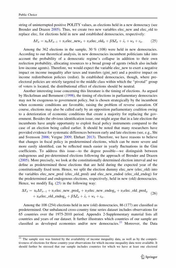
string of uninterrupted positive POLITY values, as elections held in a new democracy (see
Brender and Drazen 2005). Thus, we create two new variables elec_new and elec_old to
replace elec, for elections held in new and established democracies, respectively:
DYit ¼ a0DYit�1 þ a1elec newit þ a2elec oldit þ bDZit þ kt þ wk þ eit: ð25Þ
Among the 362 elections in the sample, 30 % (108) were held in new democracies.
According to our theoretical analysis, in new democracies incumbent politicians take into
account the probability of a democratic regime’s collapse in addition to their own
reelection probability, allocating resources to a broad group of agents (which also include
low-income agents). Therefore, we would expect the variable elec_new to exert a negative
impact on income inequality after taxes and transfers (gini_net) and a positive impact on
income redistribution policies (redist). In established democracies, though, where pre-
electoral policies are strictly targeted to the middle class within which the ‘‘pivotal’’ group
of voters is located, the distributional effect of elections should be neutral.
Another interesting issue concerning this literature is the timing of elections. As argued
by Heckelman and Berument (1998), the timing of elections in parliamentary democracies
may not be exogenous to government policy, but is chosen strategically by the incumbent
when economic conditions are favorable, raising the problem of reverse causation. Of
course, elections may also be called early by an opposition parliamentary coalition owing
to a deterioration of economic conditions that create a majority for replacing the gov-
ernment. Besides the obvious identification issue, one might argue that in a late election the
incumbents have ample opportunity to exploit fiscal policy instruments compared to the
case of an election being called earlier. It should be noted that many researchers have
provided evidence for systematic differences between early and late elections (see, e.g., Shi
and Svensson 2006; Vergne 2009; Ehrhart 2013). Therefore, we have reasons to believe
that changes in fiscal policy in predetermined elections, which can be more severe and
more easily identified, can be reflected much easier in yearly fluctuations in the Gini
coefficients. To address this issue—to the degree possible—we distinguish between
endogenous and pre-determined elections following the approach of Brender and Drazen
(2005). More precisely, we look at the constitutionally determined election interval and we
define as predetermined those elections that are held during the expected year of the
constitutionally fixed term. Hence, we split the election dummy elec_new (elec_old) into
the variables elec_new_pred (elec_old_pred) and elec_new_endod (elec_old_endog) for
the predetermined and endogenous elections, respectively, held in new (old) democracies.
Hence, we modify Eq. (25) in the following way:
DYit ¼ a0DYit�1 þ a1elec new predit þ a2elec new endogit þ a3elec old predit
þ a4elec old endogit þ bDZit þ kt þ wk þ eit:ð26Þ
Among the 108 (254) elections held in new (old) democracies, 86 (177) are classified as
predetermined. Our unbalanced cross-country time series dataset includes observations for
65 countries over the 1975-2010 period. Appendix 2-Supplementary material lists all
countries and years of our dataset. It further illustrates which countries of our sample are
classified as developed economies and/or new democracies.22 Moreover, the Data
22 The sample size was limited by the availability of income inequality data, as well as by the competi-tiveness of elections for those country-year observations for which income inequality data were available. Itshould further be stressed that our sample includes countries for which we have at least one electoral
Public Choice
123

Appendix-Supplementary material provides definitions, data sources and descriptive
statistics of all variables used in our estimations.
Regarding the econometric specification, the inclusion of the lagged dependent variable
on the right-hand side introduces a potential bias in our estimates by not satisfying the strict
exogeneity assumption of the error term eit. One solution could be the adoption of the
GMM estimator, developed for dynamic panel data (e.g., Arellano and Bond 1991;
Blundell and Bond 1998). However, these methods yield consistent estimates in small T,
large N panels. Our sample contains 65 countries, but when these are split between
developed and developing countries we actually are left with 22 and 43 cross-sections,
respectively, raising issues of consistency for the GMM method. Still, as it is analyzed in
the literature, the estimated bias of this formulation is of order 1/T, where T is the time
length of the panel, even as the number of countries becomes large (see, among others,
Nickell 1981). The average time series length of our panel is close to 22, 29, and 18
observations for the whole sample, the developed and developing countries, respectively,
likely making the bias negligible. Therefore, we estimate Eqs. (24), (25), and (26)
employing the OLS estimator with time and regional fixed effects.
4 Results
4.1 Baseline results
Our baseline results are reported in Table 1. In columns (1)–(3) we report the estimates of
Eq. (24). As can be seen, the variable elec in column (2) is negative and significantly
related to the variable Dgini_net at the 10 % level. Hence, we have some weak evidence
that net income inequality declines near elections. Next, in columns (4)–(6) we estimate
Eq. (25) splitting the election dummy into the variables elec_new and elec_old for elec-
tions in new and old democracies, respectively. Estimates for the variable elec_old indicate
that pre-electoral fiscal changes in established democracies do not have any significant
distributional implications. For the new democracies, our findings differ considerably. In
particular, in column (5) the variable elec_new is negatively related to net income
inequality at the 1 % level. Given that in column (4) market inequality does not seem to be
affected, this policy intervention in new democracies seems to act as a means of redis-
tributing income to the poorer segments of the society. Indeed, in column (6), the pre-
electoral change in market inequality owing to taxes and transfers is positive and statis-
tically significant at the 5 % level.23
Footnote 22 continuedobservation available over a 5-year period. The results remain robust, though, when we restrict the sample tothose countries for which more than ten observations are available.23 Moreover, pre-electoral manipulation of fiscal policy, and its distributional implications, may dependsignificantly on the nature of the constitutional rules. As outlined by the relevant literature, politicians inproportional and parliamentary democracies are more prone to promote broad-based policies, such aswelfare spending, while in majoritarian and presidential regimes this holds for geographically targetedexpenditures (see, e.g., Milesi-Ferretti et al. 2002; Persson and Tabellini 2003). Hence, electoral cycles maydiffer significantly between proportional and majoritarian systems or presidential and parliamentary gov-ernments. It is worth noting, though, that when we split the election dummy to account for these differences,the results (available upon request) suggest that the constitutional rules matter, but only for new democracieswherein the electoral cycle exists to begin with.
Public Choice
123

Ta
ble
1Electionsandfiscal
redistribution:basic
findings
Dependentvariable
(1)
(2)
(3)
(4)
(5)
(6)
(7)
(8)
(9)
Dgini_market
Dgini_net
Dredist
Dgini_market
Dgini_net
Dredist
Dgini_market
Dgini_net
Dredist
elec
-0.038
-0.088*
0.132
(0.07)
(0.04)
(0.09)
elec_new
-0.018
-0.248***
0.638**
(0.13)
(0.09)
(0.26)
elec_old
-0.047
-0.018
-0.088
(0.07)
(0.04)
(0.08)
elec_new
_pred
0.050
-0.270***
0.863***
(0.13)
(0.10)
(0.30)
elec_new
_endog
-0.281
-0.164
-0.204
(0.34)
(0.24)
(0.36)
elec_old_pred
-0.031
-0.010
-0.028
(0.07)
(0.05)
(0.09)
elec_old_endog
-0.097
-0.056
-0.209
(0.18)
(0.08)
(0.25)
DYt-
10.220**
0.191**
0.179**
0.220**
0.194**
0.180***
0.222***
0.192**
0.183***
(0.08)
(0.09)
(0.07)
(0.08)
(0.09)
(0.07)
(0.08)
(0.09)
(0.07)
Dgdppc
0.149
0.036
0.166
0.149
0.033
0.180
0.143
0.033
0.157
(0.09)
(0.08)
(0.12)
(0.09)
(0.08)
(0.12)
(0.09)
(0.08)
(0.12)
Dgdppc^2
-0.001
-0.000
-0.002*
-0.001
-0.000
-0.002*
-0.001
-0.000
-0.002*
(0.00)
(0.00)
(0.00)
(0.00)
(0.00)
(0.00)
(0.00)
(0.00)
(0.00)
Dhuman
capital
-0.006
-2.182
2.773
-0.001
-2.220
2.904
0.010
-2.210
2.934
(2.57)
(2.03)
(2.50)
(2.57)
(2.05)
(2.51)
(2.57)
(2.04)
(2.53)
Ddependency
0.128
0.069
0.075
0.128
0.068
0.077
0.126
0.067
0.075
(0.09)
(0.08)
(0.10)
(0.09)
(0.07)
(0.10)
(0.09)
(0.07)
(0.11)
Public Choice
123

Ta
ble
1continued
Dependentvariable
(1)
(2)
(3)
(4)
(5)
(6)
(7)
(8)
(9)
Dgini_market
Dgini_net
Dredist
Dgini_market
Dgini_net
Dredist
Dgini_market
Dgini_net
Dredist
Dpopulation_density
0.047*
0.006
0.075***
0.046*
0.008
0.070***
0.045*
0.008
0.066***
(0.02)
(0.02)
(0.02)
(0.02)
(0.02)
(0.02)
(0.02)
(0.02)
(0.02)
Dinflation
0.019
0.025*
-0.018
0.019
0.026*
-0.020
0.018
0.026*
-0.024
(0.02)
(0.01)
(0.02)
(0.02)
(0.01)
(0.02)
(0.02)
(0.01)
(0.02)
Dglobal
0.029
0.027**
-0.012
0.029
0.027**
-0.010
0.029
0.027**
-0.011
(0.02)
(0.01)
(0.03)
(0.02)
(0.01)
(0.03)
(0.02)
(0.01)
(0.03)
R2
0.131
0.132
0.086
0.131
0.135
0.094
0.132
0.135
0.099
N1421
1421
1421
1421
1421
1421
1421
1421
1421
Avg.timeseries
length
21.9
21.9
21.9
21.9
21.9
21.9
21.9
21.9
21.9
TheDprefixofavariableindicates
thatthefirstdifferencesweretaken.Allregressionsincludetimeandregionalfixed
effects.Robuststandarderrors,clustered
bycountryare
reported
inparentheses
***denotessignificance
at1%
level,**denotessignificance
at5%
level
and*denotessignificance
at10%
level
Public Choice
123

Next, in columns (7)–(9), we proceed to the estimation of Eq. (26), where our election
dummies distinguish between pre-determined and endogenous elections held either in new
or in old democracies.24 Once again, we do not obtain any statistically significant effect for
elections held in established democracies. Moreover, for new democracies, results for the
variable elec_new_pred seem to be consistent with those obtained in the previous speci-
fication for the variable elec_new. This suggests that only in predetermined pre-electoral
campaigns in new democracies, fiscal policy manipulation promotes fiscal redistribution.25
This is the expected result, since fiscal policy changes in a late election, which can be more
severe and/or more easily identified than in the case of an early election, are reflected in
changes in fiscal redistribution.
These empirical findings are consistent with our theoretical predictions as well as with
previous studies on the same subject (see, e.g., Brender and Drazen 2008, 2009). More
precisely, consistent with our theory, in new democracies where an election can be held ‘‘in
the shadow of revolution’’, fiscal redistribution can act as a device to consolidate
democracy. Our findings are also in accordance with those of Brender and Drazen
(2008, 2009), who suggest that in new democracies pre-electoral shifts in fiscal policy do
not serve to improve reelection prospects. Instead, the same authors provide evidence that
newly established regimes are almost three times more likely to collapse in election years
than in non-election years. They conclude that incumbent politicians in new democracies
provide benefits mostly because they seek to provide a signal that ‘‘democracy works’’ and
therefore prevent a reversion to autocracy at a time of high vulnerability.
4.2 Economic development, regime maturity, and elections
Several papers in the literature have reported evidence that electoral cycles are driven, or at
least amplified, by the experience of less developed countries (see, e.g., Klomp and de
Haan 2013b; Streb and Torrens 2013). According to Schuknecht (1996), fiscal manipu-
lation is more likely in developing countries because checks and balances are weaker,
allowing for greater political discretion over policy instruments. Moreover, Shi and
Svensson (2006) argue that information asymmetries between voters and politicians
regarding the competence level of the latter—a crucial assumption of PBC models—are
more pronounced in developing countries. According to this view, as the number of voters
who fails to distinguish election-motivated fiscal policy manipulations from incumbent
competence increases, the more the incumbent can benefit from opportunistic behaviors
before an election. In contrast, in developed countries where well-informed voters can
evaluate more accurately a government’s performance (competence), pre-electoral fiscal
manipulation seems to be punished rather rewarded at the polls (see, e.g., Peltzman 1992;
Brender and Drazen 2008).
Therefore, our next task would be to access if the level of development can overshadow
the observed systematic differences between new and established democracies. To this end,
24 Moreover, to check whether government ideology and its effect on fiscal policy priorities (see, e.g.,Hibbs, 1977; Potrafke, 2011) affects our results, we have interacted the electoral dummy variables in newand old democracies with a dummy variable that takes the value of one for left wing governments and 0otherwise. Our results (available upon request) do not suggest that fiscal redistribution in ‘‘young democ-racies’’ is conditional on government ideology.25 As already mentioned, following the approach of Brender and Drazen (2005), we consider the first fourelections after a shift to a democratic regime as elections held in a new democracy. Alternatively, if wereduce this cut-off point to three elections our results remain essentially the same, whereas if we increase itto five, as expected, the effect becomes weaker.
Public Choice
123

in Table 2 we re-estimate the specification in Eq. (26), as in columns (7)–(9) of Table 1,
after splitting the sample between developed and developing countries. With respect to
developed countries, the coefficient of the variable elec_new_pred is negatively and sig-
nificantly related to market income inequality, which contributes to the significant
reduction of net inequality. However, this change does not seem to emerge from the tax-
transfer system, leaving our measure of fiscal redistribution in column (3) unaffected. It is
worth mentioning, though, that we cannot make strong inferences about this result, since
we have only eight election observations for this variable. Results for the other three
electoral variables in columns (1)–(3), namely elec_new_endog, elec_old_pred and
elec_old_endog, do not reveal any other significant effect. Turning to developing countries,
as can be seen in columns (4)–(6) of Table 2, results for the variable elec_new_pred are
consistent with those obtained for the whole sample in Table 1. Concerning the magnitude
of the effect of predetermined elections in new democracies, we observe in column (6) an
increase in the change of fiscal redistribution by 0.88 points. Given that the mean value of
Dredist in the sample is 0.034 points (with a standard deviation of 1.7 points), it is clear
that this effect is quantitatively sizable. Results for the rest electoral variables in columns
(4)–(6) are statistically insignificant, indicating that the age of the regime and not the level
of development is what matters for our findings.
Table A2 in the Supplementary material presents an alternative specification where we
split the sample, not the election dummy, between new and established democracies in
developed and developing countries. In all sub-samples of Table A2 we apply the simple
specification of Eq. (24), where additionally we split the election dummy between pre-
determined (elec_pred) and endogenous elections (elec_end) to account for the potential
endogeneity of the electoral process.26 Moreover, given that the average length of the panel
in some cases drops below 11, we opt for applying Bruno’s (2005) bias corrected least
squares dummy variable estimator for dynamic panel data models with small N. Our results
seem to verify those obtained in Table 2.
4.3 Regime’s stability and fiscal redistribution around elections
According to our theoretical analysis, uncertainty regarding the type of the political regime
is the driving force of our results. So far, this uncertainty has been measured by the age of
the democracy. In this section, we attempt to corroborate this theoretical prediction by
augmenting our analytical specification in Eq. (26) with proxies for political instability. To
measure regime (in)stability, we employ two measures of civil unrest as provided by the
Social, Political, and Economic Event Database (see Nardulli et al. 2011).27 The database
reports daily observations for a range of variables (e.g., coups, anti-regime protests), which
we collapse into country-year observations. From the alternatives provided, we choose the
26 It should be noted that we do not have enough observations to perform regressions for new democraciesin developed economies.27 We have to note that our measure of political instability captures social unrest events. Therefore, it maydiscount the potential negative attitude of ordinary citizens towards democracy, since it focuses solely on theextreme cases in which people revolt or protest owing to disappointment concerning the quality of theregime. Ideally, we would prefer to use variables from the World Value Survey that measure publicperception towards democracy (see Inglehart et al. 2004). Unfortunately, for the most relevant questions ofthis survey (e.g., having a democratic political system), we have only three observations per country from1994 onwards. For a more detailed discussion concerning the difficulties of measuring the ‘‘potential threatof revolution’’, which is different from the ‘‘revolutionary events’’ that actually take place, see Aidt et al.(2014).
Public Choice
123

variables state repression and state violence as the two most relevant for our purpose. A
score of zero on these intensity measures indicate a year with no reported unrest, whereas
larger values reflect greater levels of instability. Hence, we augment Eq. (26) with inter-
action terms of the electoral variables (e.g., elec_new_pred 9 Dinstability), where Din-stability refers to the first difference of the two proxy variables described above. For
brevity, in Table 3 we report estimates only for the main outcome measure of interest,
namely the variable Dredist. In columns (1)–(3), the estimates refer to the whole sample,
developed and developing countries, respectively, when state repression is used as the
proxy for political instability. Columns (4)–(6) have the same structure when state violence
is entered alternatively.
Table 2 Elections and fiscal redistribution: developed vs. developing countries
Dependent variable Developed countries Developing countries
(1) (2) (3) (4) (5) (6)Dgini_market Dgini_net Dredist Dgini_market Dgini_net Dredist
elec_new_pred -0.790** -0.734* 0.051 0.087 -0.249** 0.886***
(0.33) (0.38) (1.79) (0.11) (0.10) (0.29)
elec_new_endog -0.332 -0.159 -0.198 -0.214 -0.175 -0.153
(0.26) (0.15) (0.40) (0.34) (0.24) (0.44)
elec_old_pred -0.019 0.000 -0.031 -0.009 0.047 -0.051
(0.09) (0.07) (0.11) (0.13) (0.09) (0.18)
elec_old_endog 0.010 0.038 -0.257 -0.270 -0.259 -0.045
(0.23) (0.09) (0.33) (0.27) (0.16) (0.36)
DYt-1 0.339*** 0.352*** 0.254*** 0.138 0.129 0.154
(0.07) (0.07) (0.06) (0.11) (0.10) (0.09)
Dgdppc 0.116 -0.018 0.218 0.452* 0.228 0.230
(0.13) (0.09) (0.14) (0.24) (0.25) (0.40)
Dgdppc^2 -0.001 0.000 -0.002* -0.012* -0.006 -0.005
(0.00) (0.00) (0.00) (0.01) (0.01) (0.01)
Dhuman capital 2.732 0.839 4.497 -2.876 -5.096 1.662
(3.02) (1.29) (4.26) (3.92) (3.31) (3.63)
Ddependency 0.144 0.016 0.152 0.069 0.047 0.047
(0.10) (0.07) (0.12) (0.12) (0.12) (0.15)
Dpopulation_density 0.003 0.001 0.006 0.067*** 0.014 0.089***
(0.03) (0.02) (0.04) (0.02) (0.02) (0.02)
Dinflation 0.541 0.487 -0.529 0.018 0.027** -0.027
(2.87) (1.80) (1.64) (0.02) (0.01) (0.02)
Dglobal 0.036 0.046* -0.075** 0.027 0.022 0.002
(0.05) (0.02) (0.03) (0.02) (0.01) (0.03)
R2 0.191 0.193 0.145 0.147 0.168 0.101
N 637 637 637 784 784 784
Avg. time series length 28.9 28.9 28.9 18.2 18.2 18.2
See Table 1
Public Choice
123

Ta
ble
3Elections,fiscal
redistribution,andpoliticalinstability
Instabilitymeasure
State
repression
State
violence
Allcountries
Developed
Developing
Allcountries
Developed
Developing
(1)
(2)
(3)
(4)
(5)
(6)
Dependentvariable
Dredist
Dredist
Dredist
Dredist
Dredist
Dredist
elec_new
_pred
0.993***
0.076
1.026***
0.998***
0.124
1.033***
(0.34)
(1.94)
(0.33)
(0.35)
(2.11)
(0.34)
elec_new
_endog
0.136
-0.567
0.298
0.099
-0.565
0.176
(0.36)
(0.40)
(0.48)
(0.38)
(0.44)
(0.46)
elec_old_pred
0.053
-0.023
0.166
0.046
-0.001
0.142
(0.11)
(0.13)
(0.19)
(0.11)
(0.13)
(0.19)
elec_old_endog
-0.155
-0.260
0.267
-0.078
-0.108
0.205
(0.29)
(0.37)
(0.46)
(0.24)
(0.25)
(0.45)
elec_new
_pred9
Dinstability
0.011
0.056
-0.001
0.008***
0.055
0.008**
(0.04)
(0.11)
(0.05)
(0.00)
(0.08)
(0.00)
elec_new
_endog9
Dinstability
0.148**
0.303
0.174*
0.060
-0.120
0.059
(0.07)
(0.26)
(0.11)
(0.07)
(0.13)
(0.09)
elec_old_pred9
Dinstability
-0.071*
-0.085
-0.065
0.013***
-0.099
0.018***
(0.04)
(0.10)
(0.05)
(0.00)
(0.07)
(0.01)
elec_old_endog9
Dinstability
-0.036
-0.168
0.000
0.057
0.242
-0.006
(0.04)
(0.18)
(0.03)
(0.07)
(0.26)
(0.02)
Dinstability
0.013
-0.013
0.013
-0.002*
-0.028
-0.002
(0.01)
(0.03)
(0.02)
(0.00)
(0.03)
(0.00)
DYt-
10.180**
0.254***
0.152
0.178**
0.229***
0.149
(0.07)
(0.06)
(0.11)
(0.07)
(0.06)
(0.11)
Dgdppc
0.229
0.261
0.040
0.269
0.278
0.142
(0.19)
(0.19)
(0.49)
(0.18)
(0.19)
(0.46)
Public Choice
123

Ta
ble
3continued
Instabilitymeasure
State
repression
State
violence
Allcountries
Developed
Developing
Allcountries
Developed
Developing
(1)
(2)
(3)
(4)
(5)
(6)
Dgdppc^2
-0.003
-0.003
0.004
-0.004
-0.003
0.002
(0.00)
(0.00)
(0.01)
(0.00)
(0.00)
(0.01)
Dhuman
capital
1.957
4.490
0.048
2.636
5.865
0.224
(2.69)
(4.54)
(3.57)
(3.00)
(5.60)
(3.53)
Ddependency
0.113
0.167
0.090
0.113
0.179
0.084
(0.13)
(0.15)
(0.18)
(0.13)
(0.15)
(0.19)
Dpopulation_density
0.084***
0.031
0.103***
0.086***
0.030
0.104***
(0.02)
(0.04)
(0.02)
(0.02)
(0.04)
(0.03)
Dinflation
-0.025
0.992
-0.030
-0.022
1.025
-0.026
(0.02)
(2.50)
(0.02)
(0.02)
(2.66)
(0.02)
Dglobal
-0.033
-0.090**
-0.023
-0.032
-0.104**
-0.023
(0.04)
(0.04)
(0.04)
(0.04)
(0.04)
(0.04)
R2
1134
504
630
1134
504
630
N0.106
0.154
0.110
0.107
0.165
0.110
Avg.timeseries
length
18.3
24.0
15.4
18.3
24.0
15.4
See
Table
1
Public Choice
123

As can be seen in Table 3, once again, the variable elec_new_pred enters with a positive
and statistically significant coefficient in our estimates, but only for the case of developed
countries in columns (2) and (5). Moreover, in columns (1)–(3) the variable Dstaterepression is related insignificantly to fiscal redistribution. Interestingly, it becomes sta-
tistically significant in columns (1) and (3) when interacted with the variable
elec_new_endog. In columns (4)–(6), the variable Dstate violence is negatively related to
fiscal redistribution only in the specification for the whole group of countries. More
importantly, the interaction terms elec_new_pred 9 Dstate violence and elec_old_pred
9 Dstate violence are positive and statistically significant in columns (4) and (6). In
contrast, in column (5) the respective variables for the sample of developed countries have
a neutral effect on fiscal redistribution. Therefore, political instability seems to bolster
fiscal redistribution in pre-electoral periods in the case of developing countries, and
especially for those countries within this sample that are considered to be new democra-
cies. In particular, in young democracies in the developing world, as expected, an increase
in the variable Dstate violence seems to intensify the already positive and statistically
effect of the variable elec_new_pred on fiscal redistribution. For developing ‘‘old
democracies’’ the electoral variable elec_old_pred remains statistically insignificant, and
for reasonable values of the variable Dstate violence so does the overall effect of elections.
However, this interesting finding might reflect that in some special cases the path to
consolidation might not be completed the first years of the democratic transition.
4.4 Sensitivity analysis
In this sub-section, we explore the robustness of the results obtained in Table 3 where the
analytical specification of Eq. (26) is augmented to provide evidence that regime insta-
bility matters for the observed electoral cycles. In our first robustness test, we employ an
alternative electoral indicator that allows us to control for differences in election dates
across as well as within countries. Moreover, we check if our results are influenced by
outlier observations.
4.4.1 Weighted electoral indicator
Until now, in order to capture the effect of elections, following the majority of the liter-
ature, the election dummy is equal to one in the year of the election, no matter when during
the year the election actually was held. This can be problematic, since if elections took
place early in the year then the election dummy can be capturing primarily post-electoral
effects. In contrast, if the election took place late in the year, then the dummy indeed can
capture more accurately the fiscal changes before the election (see, e.g., Brender and
Drazen 2005; Vergne 2009). For that latter case, one could also argue that Gini coefficients
can gauge more effectively the fiscal effects of elections. To address this issue, we follow
the approach of Franzese (2000), redefining our electoral variable to give more weight to
elections that took place later during the year. Therefore, our new pre-electoral variable
(preel) takes the value of x/12; with x denoting the month the election is held. In order to
reproduce the specification in Table 3, we split the variable preel into preel_new_pred
(preel_new_end) and preel_old_pred (preel_old_end), for predetermined (endogenous)
elections in new and old democracies, respectively.
As can be seen in Table 4, our most important finding that state violence during pre-
determined elections in developing countries reinforces fiscal redistribution remains
unaffected. Interestingly, the interaction term preel_old_pred 9 Dstate violence becomes
Public Choice
123

Ta
ble
4Elections,fiscal
redistributionandpoliticalinstability:alternativetimingofelections
Instabilitymeasure
State
repression
State
violence
Allcountries
Developed
Developing
Allcountries
Developed
Developing
(1)
(2)
(3)
(4)
(5)
(6)
Dependentvariable
Dredist
Dredist
Dredist
Dredist
Dredist
Dredist
preel_new
_pred
1.409***
2.167
1.306**
1.434***
2.461
1.333**
(0.49)
(5.40)
(0.50)
(0.50)
(6.18)
(0.51)
preel_new
_endog
-0.061
-0.559
0.007
-0.095
-0.577
-0.100
(0.29)
(0.51)
(0.38)
(0.32)
(0.54)
(0.40)
preel_old_pred
0.103
0.117
0.038
0.091
0.103
-0.020
(0.15)
(0.20)
(0.23)
(0.14)
(0.20)
(0.26)
preel_old_endog
-0.529
-0.642
-0.147
-0.471
-0.509*
-0.153
(0.35)
(0.40)
(0.69)
(0.31)
(0.28)
(0.65)
preel_new
_pred9
Dinstability
-0.057
0.284
-0.096
0.013**
0.200
0.012*
(0.13)
(0.32)
(0.16)
(0.01)
(0.24)
(0.01)
preel_new
_endog9
Dinstability
0.168
0.330
0.144
0.032
-0.123
0.010
(0.13)
(0.35)
(0.18)
(0.07)
(0.17)
(0.08)
preel_old_pred9
Dinstability
-0.073
-0.067
-0.072
0.010*
-0.384**
0.020**
(0.07)
(0.23)
(0.09)
(0.00)
(0.18)
(0.01)
preel_old_endog9
Dinstability
-0.081
-0.204
-0.029
0.147
0.426
-0.015
(0.10)
(0.32)
(0.06)
(0.15)
(0.35)
(0.03)
Dinstability
0.013
-0.025
0.015
-0.002
-0.027
-0.001
(0.01)
(0.03)
(0.02)
(0.00)
(0.03)
(0.00)
DYt-
10.176**
0.249***
0.143
0.172**
0.229***
0.137
(0.07)
(0.06)
(0.11)
(0.07)
(0.06)
(0.11)
Dgdppc
0.246
0.235
0.111
0.270
0.268
0.145
(0.19)
(0.18)
(0.49)
(0.19)
(0.18)
(0.47)
Public Choice
123
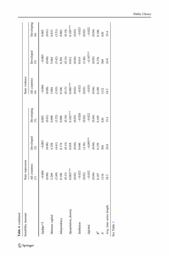
Ta
ble
4continued
Instabilitymeasure
State
repression
State
violence
Allcountries
Developed
Developing
Allcountries
Developed
Developing
(1)
(2)
(3)
(4)
(5)
(6)
Dgdppc^2
-0.004
-0.003
0.002
-0.004
-0.003
0.002
(0.00)
(0.00)
(0.01)
(0.00)
(0.00)
(0.01)
Dhuman
capital
2.269
4.258
0.690
3.084
5.664
0.833
(2.69)
(4.61)
(3.52)
(3.03)
(5.42)
(3.51)
Ddependency
0.108
0.174
0.088
0.106
0.202
0.082
(0.13)
(0.14)
(0.18)
(0.13)
(0.14)
(0.18)
Dpopulation_density
0.082***
0.018
0.102***
0.086***
0.012
0.105***
(0.02)
(0.04)
(0.03)
(0.02)
(0.04)
(0.03)
Dinflation
-0.023
0.646
-0.026
-0.021
0.614
-0.023
(0.02)
(2.36)
(0.02)
(0.02)
(2.46)
(0.02)
Dglobal
-0.032
-0.093**
-0.022
-0.033
-0.107**
-0.022
(0.04)
(0.04)
(0.04)
(0.04)
(0.05)
(0.04)
R2
0.107
0.159
0.105
0.109
0.176
0.106
N1134
504
630
1132
504
630
Avg.timeseries
length
18.3
24.0
15.4
18.3
24.0
15.4
See
Table
1
Public Choice
123

negative and statistically significant at the 5 % level in column (5). Hence, our findings
indicate that instability around predetermined elections weakens fiscal redistribution in
established developed democracies. However, since this empirical result is far from being
robust we do not seek to provide any formal theoretical intuition.
4.4.2 Testing for outliers
Our next step is to perform two checks in order to ensure that our results are not influenced
by outlier observations. First, to control for the effect of individual outliers, we use Cook’s
distance, which measures the effect of deleting a given observation based on each
observation’s residual in the regression and its leverage in the estimation process. Hence,
according to the rule of thumb, we re-estimate our preferred specifications after dropping
observations with a Cook’s distance larger than 4/n (where n the number of observations).
Second, as already mentioned, the SWIID maximizes the comparability of available
income inequality data, but incomparability remains and is reflected in the standard errors
reported for each observation of variables gini_market, gini_net, and redist. The provision
of standard errors is an additional advantage of the SWIID, because a large part of the
remaining uncertainty of inequality data estimates can be taken into account. Therefore, in
order to increase the reliability of our results further, we drop from regressions 10 % of the
observations for which the variables gini_market, gini_net, and redist are associated with
larger standard errors. In columns (1)–(6) of Table 5 we repeat the estimates of Table 3
after applying Cook’s criterion, whereas in the second half of Table 5 we alternatively drop
from the same estimates the most noisy inequality data.
As can be seen, apart from the interesting finding that the interaction term elec_
new_pred 9 Dstate repression is positive and significantly related to fiscal redistribution
for the sample of developing countries in columns (3) and (6), our results are in line with
those reported in Table 3.28
To sum up, our results clearly support the link between pre-electoral redistribution and
instability, especially when the latter is proxied by the intensity of state violence. Inter-
estingly, our findings also reveal that in some special cases incumbents in developing ‘‘old
democracies’’ might implement fiscal redistribution around elections, indicating that the
path to consolidation might not be completed during the first years of the democratic
transition. It should be noted that in Tables A3 and A4 of the Supplementary material, we
perform the same robustness checks for the specification in Table 2 and results remain
unaffected.
To close, we discuss our empirical findings concerning the rest of the covariates in
Tables 1, 2, 3, 4, and 5. First of all, the lagged dependent variable, as expected, bears a
positive and significant coefficient in the large majority of our estimates. Moreover, we get
some weak evidence that GDP per capita has the expected hump-shaped relationship with
market inequality for the sample of developing countries. Moreover, in accordance with
our theoretical priors, the coefficient of the variable Dpopulation_density is positive when
significantly related to market inequality and fiscal redistribution. Next, Dinflation enters
28 In additional robustness checks, we attempt to assess the importance of specific groups of countries forour results. To this end, we drop from our preferred specifications former Soviet Union countries, since theprofound restructuring of those countries’ societies and economies during the period of democratizationprobably differs significantly from other democratizations observed in our sample. Moreover, we drop fromour sample the three Sub-Saharan African countries, because we expect the accuracy of the inequality datato be thinner than in the rest of our sample. In both cases, though, our results (available upon request) remainunaffected.
Public Choice
123

Ta
ble
5Elections,fiscal
redistribution,andpoliticalinstability:excludingoutlierobservations
Instability
measure
State
repression
State
violence
State
repression
State
violence
All
countries
Developed
Developing
All
countries
Developed
Developing
All
countries
Developed
Developing
All
countries
Developed
Devel-
oping
(1)
(2)
(3)
(4)
(5)
(6)
(7)
(8)
(9)
(10)
(11)
(12)
Dependent
variable
Dredist
Dredist
Dredist
Dredist
Dredist
Dredist
Dredist
Dredist
Dredist
Dredist
Dredist
Dredist
elec_new
_pred
0.404**
-0.627*
0.538*
0.365*
-0.566
0.539*
0.671**
-1.809***
0.731***
0.690**
-1.833***
0.749***
(0.20)
(0.36)
(0.27)
(0.20)
(0.34)
(0.28)
(0.29)
(0.24)
(0.27)
(0.30)
(0.24)
(0.28)
elec_new
_endog
-0.062
-0.316
-0.108
0.067
-0.138
0.105
-0.178
0.157
-0.200
-0.108
0.084
-0.077
(0.26)
(0.35)
(0.31)
(0.25)
(0.37)
(0.31)
(0.23)
(0.31)
(0.31)
(0.25)
(0.33)
(0.30)
elec_old_pred
0.093
0.122
0.039
0.011
0.132
0.043
-0.004
0.038
0.022
-0.014
0.070
-0.001
(0.09)
(0.13)
(0.13)
(0.11)
(0.13)
(0.13)
(0.10)
(0.15)
(0.15)
(0.11)
(0.13)
(0.14)
elec_old_endog
-0.048
-0.150
0.200
-0.062
-0.115
0.197
-0.218
-0.293
0.443
-0.103
-0.143
0.372
(0.13)
(0.19)
(0.15)
(0.13)
(0.15)
(0.16)
(0.30)
(0.41)
(0.62)
(0.23)
(0.22)
(0.65)
elec_new
_pred
9Dinstability
0.032
0.001
0.075*
0.027
0.002
0.040*
-0.013
-0.069*
-0.014
0.008***
-0.030
0.009***
(0.04)
(0.06)
(0.04)
(0.02)
(0.04)
(0.03)
(0.04)
(0.04)
(0.07)
(0.00)
(0.04)
(0.00)
elec_new
_endog
9Dinstability
0.000
0.001
-0.113
0.036
0.003
-0.095
0.056
0.006
-0.085
0.060
0.017
0.070
(0.12)
(0.05)
(0.12)
(0.03)
(0.05)
(0.09)
(0.13)
(0.35)
(0.16)
(0.07)
(0.17)
(0.09)
elec_old_pred
9Dinstability
-0.003
0.053
-0.025
0.005
0.053
0.006**
-0.062
-0.064
-0.059
0.012***
-0.108
0.014***
(0.03)
(0.07)
(0.04)
(0.00)
(0.06)
(0.00)
(0.04)
(0.09)
(0.05)
(0.00)
(0.07)
(0.00)
elec_old_endog
9Dinstability
-0.035
-0.173
0.003
0.021
0.084
0.008
-0.029
-0.266**
0.008
0.090
0.162
0.006
(0.03)
(0.11)
(0.02)
(0.02)
(0.06)
(0.02)
(0.04)
(0.12)
(0.03)
(0.09)
(0.32)
(0.03)
Dinstability
0.006
0.015
0.005
-0.001
-0.013
0.001
0.009
-0.023
0.017
-0.003**
-0.020
-0.002**
(0.01)
(0.02)
(0.01)
(0.00)
(0.02)
(0.00)
(0.01)
(0.03)
(0.01)
(0.00)
(0.03)
(0.00)
DYt-
10.345***
0.418***
0.261***
0.355***
0.444***
0.257***
0.130*
0.289***
0.136
0.127*
0.273***
0.135
(0.04)
(0.04)
(0.07)
(0.05)
(0.03)
(0.08)
(0.07)
(0.05)
(0.12)
(0.07)
(0.06)
(0.12)
Dgdppc
0.140
0.442**
-0.005
0.141
0.426**
-0.100
0.291
0.324*
0.298
0.315
0.333**
0.318
(0.14)
(0.17)
(0.38)
(0.14)
(0.16)
(0.38)
(0.21)
(0.16)
(0.50)
(0.21)
(0.16)
(0.50)
Public Choice
123

Ta
ble
5continued
Instability
measure
State
repression
State
violence
State
repression
State
violence
All
countries
Developed
Developing
All
countries
Developed
Developing
All
countries
Developed
Developing
All
countries
Developed
Devel-
oping
(1)
(2)
(3)
(4)
(5)
(6)
(7)
(8)
(9)
(10)
(11)
(12)
Dgdppc^2
-0.002
-0.006**
0.004
-0.002
-0.006**
0.007
-0.003
-0.003*
-0.004
-0.004
-0.004*
-0.004
(0.00)
(0.00)
(0.01)
(0.00)
(0.00)
(0.01)
(0.00)
(0.00)
(0.01)
(0.00)
(0.00)
(0.01)
Dhuman
capital
-0.123
2.128
0.470
-0.729
2.802
0.825
2.543
4.940
-0.101
3.510
6.374
0.089
(2.03)
(2.53)
(3.03)
(1.97)
(2.33)
(3.08)
(2.89)
(4.64)
(3.84)
(3.37)
(6.23)
(3.79)
Ddependency
0.138*
0.177
0.190
0.142*
0.192
0.199
0.228*
0.206
0.202
0.225*
0.213
0.175
(0.08)
(0.11)
(0.12)
(0.08)
(0.12)
(0.12)
(0.12)
(0.14)
(0.17)
(0.12)
(0.14)
(0.17)
Dpopulation_
density
0.009
0.013
0.008
0.010
0.008
0.009
0.059
0.058**
0.066*
0.067
0.068**
0.069*
(0.01)
(0.02)
(0.01)
(0.01)
(0.03)
(0.01)
(0.04)
(0.03)
(0.04)
(0.04)
(0.03)
(0.04)
Dinflation
0.000
0.126
-0.002
-0.005
-0.226
-0.006
0.013
0.160
-0.009
0.012
0.050
-0.008
(0.01)
(1.47)
(0.01)
(0.01)
(1.46)
(0.01)
(0.03)
(2.84)
(0.01)
(0.03)
(3.28)
(0.01)
Dglobal
-0.015
-0.075**
0.015
-0.008
-0.059*
0.018
-0.041
-0.090*
-0.040
-0.041
-0.100*
-0.038
(0.02)
(0.03)
(0.02)
(0.02)
(0.03)
(0.02)
(0.04)
(0.05)
(0.05)
(0.04)
(0.05)
(0.05)
R2
0.193
0.286
0.169
0.204
0.298
0.170
0.090
0.205
0.096
0.094
0.198
0.098
N973
443
536
977
440
534
996
443
547
996
443
547
Avg.timeseries
length
27.5
27.2
27.5
17.4
17.3
17.3
26.1
26.1
26.1
16.4
16.4
16.4
TheDprefixofavariable
indicates
that
thefirstdifferencesweretaken.Allregressionsincludetimeandregional
fixed
effects.In
columns(1)–(6)werepeatestimates
of
Table
3afterdroppingobservationswithestimated
Cook’sdistance
larger
than
4/n
(wherenthenumber
ofobservations).In
columns(7)–(12)werepeatestimates
ofTable
3afterdropping10%
oftheobservationsthat
areassociated
withthehigher
uncertainty
intheinequalitydataestimates.Robust
standarderrors,clustered
bycountryare
reported
inparentheses
***denotessignificance
at1%
level,**denotessignificance
at5%
level
and*denotessignificance
at10%
level
Public Choice
123

with a positive and significant coefficient in the empirical specification when net inequality
is the dependent variable in Table 1, although this result does not seem to be robust
throughout. Finally, the variable Dglobal has a positive (negative), though not robust,
effect on net income inequality (fiscal redistribution) in developed countries.
5 Conclusions
Starting from Tullock (1974), a large strand of the political economy literature investigates
the role of the threat of revolution in triggering democratic transitions (see, e.g., Acemoglu
and Robinson 2000, 2006; Przeworski 2009; Aidt and Jensen 2014). However, most of
these studies assume that de facto political power does not play a role in policy decisions
after the transition to a democratic regime. This is because in a democratic regime all
agents recognize elections as the one and only acceptable political decision mechanism
and, hence, conflicts of interests are resolved strictly through voting. However, assuming
that de facto political power vanishes just after the transition to democracy, and treating
democratic elections as being self-enforcing, leaves unexplored a large number of inter-
esting political issues related to the transition process. Moreover, history suggests that
waves of democratization many times are followed by reverse waves to dictatorship (see,
e.g., Huntington 1993), providing anecdotal evidence that a democratic regime, especially
a new one, is far from being self-enforcing (see Fearon 2011 for a discussion on this issue).
Building on this rationale, the present paper investigates how the de facto political
power—and the consequent threat of revolution—may affect implemented economic
policies in democracies, especially during the first years of the transition. Our analysis
suggests that in relatively stable democratic regimes, income transfers are targeted strictly
to the middle class, in which the ‘‘pivotal’’ group of voters is located, leaving unaffected
the distribution of income. However, in new democracies wherein fiscal policies also serve
as a device for consolidating democratic regimes, incumbent politicians allocate resources
to a broader group of agents, thereby boosting fiscal redistribution.
Our empirical results for a sample of 65 developed and developing countries over the
1975–2010 period support these theoretical predictions. In particular, our findings indicate
that in countries characterized as young democracies, elections exert a positive and sig-
nificant impact on fiscal redistribution, as measured by the reduction in market income
inequality associated with taxes and transfers. Moreover, we find that the effect of elections
is stronger when new democracies are characterized by relatively greater political insta-
bility, especially when the latter is proxied by state violence. Backed by strong empirical
results, we contend that fiscal redistribution acts as a mean of consolidating a vulnerable
democratic regime.
Acknowledgments We have benefited from comments and suggestions by Stelios Arvanitis, GeorgeEfthyvoulou, Arne Risa Hole, Nasos Roussias, Karl Taylor, and seminar participants at the 2015 RoyalEconomic Society Conference, the 2015 Meeting of the European Public Choice Society, the 14th Con-ference on Research on Economic Theory and Econometrics and the Governance and Participation work-shop at the University of Sheffield. Last but not least, we also want to thank an anonymous referee and theeditor for many helpful comments and suggestions which led to substantial improvements in the paper. Allremaining errors are ours.
Open Access This article is distributed under the terms of the Creative Commons Attribution 4.0 Inter-national License (http://creativecommons.org/licenses/by/4.0/), which permits unrestricted use, distribution,
Public Choice
123

and reproduction in any medium, provided you give appropriate credit to the original author(s) and thesource, provide a link to the Creative Commons license, and indicate if changes were made.
References
Acemoglu, D., Johnson, S., & Robinson, J. (2005). Institutions as a fundamental cause of long-run growth.In P. Aghion & S. Durlauf (Eds.), Handbook of economic growth. Amsterdam: North Holland.
Acemoglu, D., & Robinson, J. (2000). Why did the west extend the franchise? Democracy, inequality, andgrowth in historical perspective. Quarterly Journal of Economics, 115(4), 1167–1199.
Acemoglu, D., & Robinson, J. (2006). Economic origins of dictatorship and democracy. Cambridge:Cambridge University Press.
Aidt, T., & Jensen, P. (2014). Workers of the world, unite! Franchise extensions and the threat of revolutionin Europe, 1820–1938. European Economic Review, 72, 52–75.
Aidt, T., & Mooney, G. (2014). Voting suffrage and the political budget cycle: evidence from the Londonmetropolitan boroughs 1902–1937. Journal of Public Economics, 112, 53–71.
Albanesi, S. (2007). Inflation and inequality. Journal of Monetary Economics, 54(4), 1088–1114.Alesina, A., Baqir, R., & Easterly, W. (2000). Redistributive public employment. Journal of Urban Eco-
nomics, 48(2), 219–241.Alesina, A., & Wacziarg, R. (1998). Openness, country size and government. Journal of Public Economics,
69(3), 305–321.Amendola, A., Easaw, J., & Savoia, A. (2013). Inequality in developing economies: the role of institutional
development. Public Choice, 155(1), 43–60.Arellano, M., & Bond, S. (1991). Some tests of specification for panel data: Monte Carlo evidence and an
application to employment equations. Review of Economic Studies, 58(2), 277–297.Barro, R., & Lee, J. (2013). A new data set of educational attainment in the world, 1950–2010. Journal of
Development Economics, 104, 184–198.Beck, T., Clarke, G., Groof, A., Keefer, P., & Walsh, P. (2001). New tools in comparative political
economy: The database of political institutions. The World Bank Economic Review, 15(1), 165–176.Besley, T., & Coate, S. (1991). Public provision of private goods and the redistribution of income. American
Economic Review, 81(4), 979–984.Block, S. (2002). Elections, electoral competitiveness, and political budget cycles in developing countries.
Harvard University CID Working Paper No. 78.Blundell, R., & Bond, S. (1998). Initial conditions and moment restrictions in dynamic panel data models.
Journal of Econometrics, 87(1), 115–143.Brender, A., & Drazen, A. (2005). Political budget cycles in new versus established democracies. Journal of
Monetary Economics, 52(7), 1271–1295.Brender, A., & Drazen, A. (2007). Why is economic policy different in new democracies? Affecting
attitudes about democracy. NBER Working Paper No. 13457.Brender, A., & Drazen, A. (2008). How do budget deficits and economic growth affect reelection prospects?
Evidence from a large panel of countries. American Economic Review, 98(5), 2203–2220.Brender, A., & Drazen, A. (2009). Consolidation of new democracy, mass attitudes, and clientelism.
American Economic Review, 99(2), 304–309.Bruno, G. (2005). Approximating the bias of the LSDV estimator for dynamic unbalanced panel data
models. Economics Letters, 87(3), 361–366.Choi, I. (2001). Unit root tests for panel data. Journal of International Money and Finance, 20(2), 249–272.Chong, A., Gradstein, M., & Calderon, C. (2009). Can foreign aid reduce income inequality and poverty?
Public Choice, 140(1), 59–84.Corvalan, A. (2014). The impact of a marginal subsidy on Gini indices. Review of Income and Wealth,
60(3), 596–603.Drazen, A., & Eslava, M. (2010). Electoral manipulation via voter-friendly spending: theory and evidence.
Journal of Development Economics, 92(1), 39–52.Dreher, A. (2006). Does globalization affect growth? Empirical evidence from a new index. Applied
Economics, 38(10), 1091–1110.Efthyvoulou, G. (2012). Political budget cycles in the European Union and the impact of political pressures.
Public Choice, 153(3), 295–327.Ehrhart, H. (2013). Elections and the structure of taxation in developing countries. Public Choice, 156(1),
195–211.Fearon, J. (2011). Self-enforcing democracy. Quarterly Journal of Economics, 126(4), 1661–1708.
Public Choice
123

Franzese, R. J. (2000). Electoral and partisan manipulation of public debt in developed democracies,1956–1990. In R. Strauch & J. Hagen (Eds.), Institutions, politics and fiscal policy (pp. 61–83).Dordrecht: Kluwer Academic Press.
Galasso, V., & Profeta, P. (2004). Lessons for an aging society: the political sustainability of social securitysystems. Economic Policy, 19(38), 63–115.
Hanusch, M., & Keefer, P. (2014). Younger parties, bigger spenders? Party age and political budget cycles.European Economic Review, 72, 1–18.
Heckelman, J., & Berument, H. (1998). Political business cycles and endogenous elections. SouthernEconomic Journal, 64(4), 987–1000.
Hibbs, D. (1977). Political parties and macroeconomic policy. American Political Science Review, 71(4),467–487.
Huntington, S. (1993). The third wave: democratization in the late twentieth century. Oklahoma: Universityof Oklahoma Press.
Inglehart, R., Basanez, M., Dıez-Medrano, J., Halman, L., & Luijkx, R. (2004). Human beliefs and values.Ann Arbor: University of Michigan Press.
Katsimi, M., & Sarantides, V. (2012). Do elections affect the composition of fiscal policy in developed,established democracies. Public Choice, 151(1), 325–362.
Khemani, S. (2004). Political cycles in a developing economy: effect of elections in the Indian states.Journal of Development Economics, 73(1), 125–154.
Klomp, J., & de Haan, J. (2013a). Conditional political budget cycles: a review of recent evidence. PublicChoice, 157(3–4), 387–410.
Klomp, J., & de Haan, J. (2013b). Do political budget cycles really exist? Applied Economics, 45(3),329–341.
Klomp, J., & de Haan, J. (2013c). Popular protest and political budget cycles: a panel data analysis.Economics Letters, 120(3), 516–520.
Klomp, J., & de Haan, J. (2013d). Political budget cycles and election outcomes. Public Choice, 157(1),245–267.
Kuznets, S. (1955). Economic growth and income inequality. American Economic Review, 45(1), 1–28.Levitt, S. (1997). Using electoral cycles in police hiring to estimate the effect of police on crime. American
Economic Review, 87(3), 270–290.Li, H., Squire, L., & Zou, H.-F. (1998). Explaining international and intertemporal variations in income
inequality. Economic Journal, 108(446), 26–43.Linz, J., & Stepan, A. (1996). Problems of democratic transition and consolidation: southern Europe, South
America, and post-communist Europe. Baltimore: Johns Hopkins University Press.Little, A. (2012). Elections, fraud, and election monitoring in the shadow of revolution. Quarterly Journal of
Political Science, 7(3), 249–283.Little, A., Tucker, J., & LaGatta, T. (2015). Election, protest and alternation of power. Journal of Politics,
77(4), 1142–1156.Lohmann, S. (1998). Rationalizing the political business cycle: a workhorse model. Economics and Politics,
10(1), 1–17.Maddala, S., & Wu, S. (1999). A comparative study of unit root tests with panel data and new simple test.
Oxford Bulletin of Economics and Statistics, 61(S1), 631–652.Marshall, M., Gurr, T., & Jaggers, K. (2013). Polity IV project: Political regime characteristics and tran-
sitions, 1800–2012. Vienna, VA: Center for Systematic Peace.Mechtel, M., & Potrafke, N. (2013). Electoral cycles in active labor market policies. Public Choice, 156(1),
181–194.Milesi-Ferretti, G. M., Perotti, R., & Massimo, R. (2002). Electoral systems and public spending. Quarterly
Journal of Economics, 117(2), 609–657.Nardulli, P., Leetaru, K., & Hayes, M. (2011). Event data, civil unrest and the social, political and economic
event database (SPEED) project: post World War II trends in political protests and violence. Quebec:Paper presented at the Annual meeting of the International Studies Association.
Nickell, S. (1981). Biases in dynamic models with fixed effects. Econometrica, 49(6), 1417–1426.Nordhaus, W. (1975). The political business cycle. Review of Economic Studies, 42(2), 169–190.Olson, M. (1965). The logic of collective actions. Public goods and the theory of groups. Cambridge:
Harvard University Press.Peltzman, S. (1992). Voters as fiscal conservatives. Quarterly Journal of Economics, 107(2), 327–361.Persson, T., & Tabellini, G. (2000). Political economics: explaining economic policy. Cambridge: MIT
Press.Persson, T., & Tabellini, G. (2003). The economic effect of constitutions. Cambridge: MIT Press.
Public Choice
123
Potrafke, N. (2011). Does government ideology influence budget composition? Empirical evidence fromOECD countries. Economics of Governance, 12(2), 101–134.
Przeworski, A. (2009). Conquered or granted? A history of suffrage extensions. British Journal of PoliticalScience, 39(2), 291–321.
Psacharopoulos, G. (1994). Returns to investment in education: a global update. World Development, 22(9),1325–1343.
Rodrik, D. (1997). Has globalization gone too far?. Institute for International Economics: Washington D.C.Rodrik, D. (1998). Do more open economies have bigger governments? Journal of Political Economy,
106(5), 997–1032.Rogoff, K. (1990). Equilibrium political budget cycles. American Economic Review, 80(1), 21–36.Schuknecht, L. (1996). Political business cycles and fiscal policies in developing countries. Kyklos, 49(2),
155–170.Schuknecht, L. (2000). Fiscal policy cycles and public expenditure in developing countries. Public Choice,
102(1–2), 115–130.Shi, M., & Svensson, J. (2006). Political budget cycles: do they differ across countries and why? Journal of
Public Economics, 90(8–9), 1367–1389.Solt, F. (2009). Standardizing the world income inequality database. Social Science Quarterly, 90(2),
231–242.Streb, J., Lema, D., & Torrens, G. (2009). Checks and balances on political budget cycles: cross country
evidence. Kyklos, 62(3), 425–446.Streb, J., & Torrens, G. (2013). Making rules credible: divided government and political budget cycles.
Public Choice, 156(3–4), 703–722.Tullock, G. (1974). The social dilemma: the economics of war and revolution. Blacksburg: Center for Study
of Public Choice.Vergne, C. (2009). Democracy, elections and allocation of public expenditures in developing countries.
European Journal of Political Economy, 25(1), 63–77.von Weizsacker, R. (1996). Distributive implications of an aging society. European Economic Review,
40(3–5), 729–746.
Public Choice
123