fiscal equity: distributional impacts of taxation and social
TRANSCRIPT
October, 2013Working Paper number 115
FISCAL EQUITY: DISTRIBUTIONAL IMPACTSOF TAXATION AND SOCIAL SPENDINGIN BRAZIL
International
Centre for Inclusive Growth
Fernando Gaiger SilveiraInstitute for Applied Economic Research (IPEA)
Fernando RezendeBrazilian School of Public and Business Administration - EBAPE/FGV
Jose Roberto AfonsoIBRE/FGV
Jhonatan FerreiraSAS Institute Brazil

Copyright© 2013International Policy Centre for Inclusive GrowthUnited Nations Development Programme
The International Policy Centre for Inclusive Growth is jointly supported by theUnited Nations Development Programme and the Government of Brazil.
Rights and Permissions
All rights reserved.
The text and data in this publication may be reproduced as long as the source is cited.Reproductions for commercial purposes are forbidden.
International Policy Centre for Inclusive Growth (IPC - IG)United Nations Development Programme
SBS, Quadra 1, Bloco J, Ed. BNDES, 13º andar70076-900 Brasilia, DF - BrazilTelephone: +55 61 21055000
E-mail: [email protected] URL: www.ipc-undp.org
The International Policy Centre for Inclusive Growth disseminates the findings of its workin progress to encourage the exchange of ideas about development issues. The papers aresigned by the authors and should be cited accordingly. The findings, interpretations, andconclusions that they express are those of the authors and not necessarily those of theUnited Nations Development Programme or the Government of Brazil.
Working Papers are available online at www.ipc-undp.org and subscriptions can be requestedby email to [email protected]
Print ISSN: 1812-108X

ACRONYMS AND ABBREVIATIONS
ANSS Agência Nacional de Saúde Suplementar (National Supplementary Health Insurance Agency)
BPS Benefício de Prestação Continuada (Continued Cash Benefit)
CIDE Contribuição e Intervenção no Domínio Econômico (Contribution to Intervene in the Economic Domain)
Cofins Contribuição Social para o Financiamento da Seguridade Social (Social Contribution for the Funding of Social Security)
CPMF Contribuição Provisória sobre a Movimentação ou Transmissão de Valores e de Créditos e Direitos de Natureza Financeira (Financial Transaction Tax)
FGTS Fundo de Garantia por Tempo de Serviço (Guarantee Fund for Employees based on Time of Service)
GDP Gross domestic product
IBGE Instituto Brasileiro de Geografia e Estatística (Brazilian Institute of Geography and Statistics)
ICMS Imposto sobre Operações Relativas à Circulação de Mercadorias e Serviços de Transporte Interestadual e Intermunicipal e de Comunicações (Tax on Operations Relating to the Distribution of Goods, Interstate and Intermunicipal Transport Services and Communications)
Inep Instituto Nacional de Estudos e Pesquisas Educacionais (National Institute for Educational Studies and Research)
INSS Instituto Nacional de Seguro Social (National Social Security Institute)
IOF Imposto sobre Operações Financeiras (Tax on Financial Operations)
IPI Imposto sobre Produtos Industrializados (Tax on Industrial Products)
IPTU Imposto sobre a Propriedade Predial e Territorial Urbana (Tax on Urban Property)
IPVA Imposto sobre a Propriedade de Veículos Automotores (Motor Vehicle Tax)
IR Imposto de Renda (Individuals’ Income Tax)
IRPF Imposto de Renda de Pessoas Físicas (Personal Income Tax)
2 International Policy Centre for Inclusive Growth
IRPJ Imposto de Renda de Pessoa Jurídica (Corporate Revenue Tax)
ISS Imposto sobre Serviços (Tax on Services)
ITBI Imposto sobre a Transmissão inter Vivos de Bens Imóveis (Tax on the Transfer of Property in Life)
ITCD Imposto De Transmissão Causa Mortis (Inheritance and Donation Tax)
LOAS Lei Orgânica de Assistência Social (Social Assistance Law)
MDS Ministério do Desenvolvimento Social e Combate à Fome (Ministry for Social Development and Combating Hunger)
PAB Piso de Atenção Básica (Basic Care Floor)
PBF Programa Bolsa Família (Bolsa Família Programme)
PIS/Pasep Contribuição para os Programas de Integração Social e de Formulação do Patrimônio do Servidor Público (Contribution for Social Integration and Public Servant Programmes)
PNAD Pesquisa Nacional de Amostra de Domicílios (National Household Sample Survey)
POF Pesquisas de Orçamentos Familiares (Household Budget Surveys)
Proesf Programa de Estruturação do Programa Saúde da Família (Programme for Structuring the Family Health Programme)
PSF Programa Saúde da Família (Family Health Programme)
RGPS Regime Geral de Previdência Social (General Regime of Social Security)
RPPS Regimes Próprios de Previdência Social (Pension Regime for Government Workers)
Siops Sistema de Gastos em Saúde (Health Spending System)
SUS Sistema Único de Saúde (Unified Health System)
Working Paper 3
FISCAL EQUITY: DISTRIBUTIONAL IMPACTS OF TAXATION
AND SOCIAL SPENDING IN BRAZIL
Fernando Gaiger Silveira; Fernando Rezende; Jose Roberto Afonso; and Jhonatan Ferreira*
1 INTRODUCTION
In 2009, the Brazilian public sector — actually, the Union: including states, municipalities and the Federal District — collected approximately 35 per cent of the gross domestic product (GDP) in taxes, and ‘gave back’ around 15 per cent in pension and health benefits to the private sector and a substantially lower amount through subsidies. Approximately one third of this amount is used to pay the pensions of public servants. Consumption expenditures reached nearly 20 per cent of GDP, while expenditure on investment — ‘gross fixed capital’ — and the net interest payments to holders of government bonds accounted for 2.3 per cent and 5.4 per cent, respectively. Also of note in public budgets are the expenditures on education and health policies, which accounted for about 9 per cent of GDP in 2009.
The analysis presented in this article shows the importance of assessing the distributional impacts on household income of taxes, social security and assistance transfers and the public provision of goods and services in education and health. That is the purpose of this study: to evaluate how primary household income changes through the intervention of social security and assistance, fiscal and public health and education policies.
We will demonstrate regressive traits of Brazilian taxation by drawing on a variety of data sources. The work considers the latest Household Budget Surveys (Pesquisas de Orçamentos Familiares — POF) undertaken by the Brazilian Institute of Geography and Statistics (IBGE) in 2002–2003 and 2008–2009, as previously evidenced by Vianna et al. (2000) in metropolitan areas, based on the 1995–2006 POF, and Silveira (2008; 2010) and Pinto-Payeras (2010) for the 2002–2003 POF.
* Fernando Gaiger Silveira, Agronomist (Esalq-USP), Doctor of Economics (Unicamp) and researcher at IPEA; Fernando Rezende, Economist, professor at the Brazilian School of Public and Business Administration - EBAPE and the Getúlio Vargas Foundation (FGV) and consultant. Former president of the Institute of Applied Economic Research – IPEA; Jose Roberto Afonso, Economist, with a doctorate degree from UNICAMP and a Master's degree from UFRJ, researcher at IBRE/FGV and technical consultant for the Federal Senate; and Jhonatan Ferreira, Bachelor in Statistics (University of Brasilia), Specialist in Applied Statistics (Cruzeiro do Sul University). Pre-sales Consultant at SAS Institute Brazil Estatistico.
This work was supported by CNPq.

4 International Policy Centre for Inclusive Growth
Innovations include deepening the distributional impacts of social spending as a result of both its growth as well as its increasing progressivity. Effectively, spending on social security and assistance, health care and public education has grown significantly in these five to six years between POFs, increasing its share by 9 per cent relative to income. However, in fact, what stands out in the share of welfare and assistance transfers and cash benefits aimed at reducing inequality is the concentration effect (i.e. the behaviour of the concentration coefficient). In concrete terms, social spending accounted for a 42 per cent drop in inequality in so-called final income,1 with the concentration effect accounting for two thirds of this contribution. Taxes accounted for only 5 per cent of the drop in inequality in final income; the behaviour of private incomes was responsible for 53 per cent of this decrease. In the case of taxes, the concentration effect has a unique role in direct taxation, while the participation effect stands out in indirect taxation.
Increased levels of social spending in Brazil have been noted by scholars of government spending— according to IPEA estimates on federal social spending, its share of GDP increased from 13.0 per cent to 15.8 per cent between 2003 and 2009. The spending considered here, with social security and assistance benefits and public education and health, has increased from 11.9 per cent of GDP in 2003 to 13.6 per cent in 2009, representing approximately 90 per cent of federal social expenses. This share should be even greater for public social spending, since spending on health and education stands out in states and municipalities.
FIGURE 1
Evolution of Brazilian Federal Spending as a Share of GDP, 2002–2009
Source: Gobetti and Orair (2010).

Working Paper 5
Another contribution from IPEA that corroborates the growth in spending on social security and public provision is shown in Figure 1. Between 2002 and 2009, there was a 2 per cent increase in the share of GDP devoted to the General Regime of Social Security (Regime Geral de Previdência Social — RGPS) social security and assistance benefits, and a 0.5 per cent increase in spending related to health and education.
In the case of taxation, despite the continuation of its regressive nature on personal income, two important distributional changes have occurred. First, the split between direct and indirect taxes has changed. Indirect taxes have decreased in importance, which reduces the regressive effect of taxation. Effectively, the share of indirect taxes decreased from 17.6 per cent to 15.5 per cent of income between 2003 and 2009, while direct taxation grew by 0.4 per cent. This increase in direct taxation, though small, is due to the growth of the formal labour market seen in recent years, which leads to an increase in the amount of social security contributions. According to the POF, direct taxes grew from 3.0 per cent to 3.3 per cent of income between 2003 and 2009 — it should be noted that this only considers the employees’ share of social security contributions. This growth can be seen in Figure 2, which shows the evolution of the make-up of the tax burden, with special emphasis on the taxes under assessment here — i.e. those levied on household income and consumption.
FIGURE 2
Evolution of the Make-up of the Tax Burden in Brazil, 2003 and 20092
Source: Internal Revenue Service.
Notes: Imposto sobre Serviços (ISS) is a municipal tax applied to the services provided to a third party by a company or professional and is paid by the service provider; Contribuição e Intervenção no Domínio Econômico (CIDE) corresponds to the economic domain intervention contribution and applies to royalty payments, technology transfers and compensation of technology supply and technical assistance; Contribuição Social para o Financiamento da Seguridade Social (Cofins) is a state tax paid by companies that collect taxes based on added value; Imposto sobre Produtos Industrializados (IPI) is applied to the output of national goods from the factory, to customs clearance when the product comes from abroad and to public sales; Imposto sobre Operações Relativas à Circulação de Mercadorias e Serviços de Transporte Interestadual e Intermunicipal e de Comunicações (ICMS) is a value-added tax on sales and services and applies to the movement of goods, transportation and communication services, and to the supply of any goods; Contribuições previdenciárias = Social security payments; Imposto sobre a Propriedade de Veículos Automotores (IPVA) is a vehicle tax applied to the possession of motorised vehicles; Imposto sobre a Propriedade Predial e Territorial Urbana (IPTU) is a municipal property tax applied to property located within urban limits; Imposto de Renda de Pessoas Físicas (IRPF) is the personal income tax that each person is required to deduct from their annual income.

6 International Policy Centre for Inclusive Growth
Social security contributions increased their share of the Brazilian tax burden from 6.1 per cent to 6.9 per cent between 2003 and 2009. Indirect taxation experienced a reduction of almost 5 per cent, while direct taxation accounted for 55.6 per cent of the burden in 2009. It is important to emphasise that the taxes reviewed in this study account for 61.0 per cent of the total tax burden. The following were left out of our measurements: corporate income tax, the employers’ share of social security contributions, the Guarantee Fund for Employees based on Time of Service (Fundo de Garantia por Tempo de Serviço — FGTS), the Social Contribution on Net Income, the Temporary Contribution on Financial Transactions, the Inheritance and Donation Tax , (Imposto De Transmissão Causa Mortis — ITCD), the Tax on the Transfer of Property in Life (Imposto sobre a Transmissão inter Vivos de Bens Imóveis — ITBI), the education allowance, contributions to the S System (Sistema S – SENAI SENAC, SEESC SENAR, etc) among other direct taxes, and the Tax on Financial Operations (Imposto sobre Operações Financeiras — IOF) and the Tax on Foreign Trade, among indirect taxes.
In discussions on taxes and social spending, two issues (or problems) are voiced by most politicians, journalists, opinion leaders, researchers and academics. On the one hand, it is believed that the tax burden in Brazil is too high and that the return, via public policy, falls far too short of what taxpayers contribute. This burden, the argument holds, is unfair; poor people pay much more, as a proportion of their income, than rich people. As a corollary to this consensus, there is a demand for lower taxes so that there may be more income and consumption. This cause is strongly backed by the middle class and, according to certain analysts, is shared by the new middle class, a stratum of the population that has reached a new income level and has increased and improved consumption patterns in the durable goods market.
In fact, the Brazilian tax burden is set at a level much higher than that observed in countries with similar per capita income levels. There are many bottlenecks in the public provision of education, health and safety, among other areas. This mismatch between what is paid and what is delivered is reflected, according to some analysts, in the demand for lower taxes and, consequently, an increase in disposable income for consumption. The book by Alberto Carlos de Almeida, O dedo na ferida: menos imposto, mais consumo (unofficial translation: ‘Salt in the wound: lower taxes, more consumption’) goes in that direction; it concludes, based on opinion polls, that the Brazilian population wants a tax break, even if it means a stagnation — or even a reduction — of public spending, particularly social spending. Indeed, the question that asks the respondent about his/her choice in the trade-off between lower taxes and more public spending does not clearly explain that lowering taxes may lead to a decline in social spending. This is because it uses the reduction in the number of civil servants exclusively as a proxy for the drop in spending. Actually, the choice is between reducing taxes with a reduction in the number of civil servants or higher taxes with an increase in social programmes. The most likely short- and medium-term effect of decreased spending is reduced social spending and public investment. Another question which sought to assess the trade-off between increased social spending and tax cuts investigates who the interviewee would choose as president — one who increased the Bolsa Família Programme (PBF) or one who reduced the tax on food so that it would become cheaper. Once again, it is not clear that the option of reducing taxes would result in a reduction in spending on the PBF or on social spending as a whole. What is surprising is that about one third of the population say they prefer a tax increase to expand social programmes.3 In terms of candidates’ profiles, it is noteworthy that, among the poorest people, earning up to one minimum wage, one third prefer higher spending on the PBF, which implicitly means an increase in taxes.
Working Paper 7
The number of people sharing this opinion decreases as income increases — among those earning more than 15 minimum wages, no one chose this response.
Carlos de Almeida then evaluates what he calls the ‘desire for autonomy’. According to the author, it relates to the idea that “People who wish for more individual autonomy prefer lower taxes and having money to pay for private health insurance” (Almeida, 2010: 79). In summary, the question in this assessment presents the following dilemma: does the respondent prefer that the government continue to tax and transfer resources through social programmes or does he/she believe that a tax reduction with a consequent increase in disposable income is more appropriate? Again, two thirds of the population want a smaller government. In this regard, there were no substantial differences across educational levels and regions. We conclude, then, that “the majority of Brazilians of all social classes would like to have more money and decide how it should be used.”
The entire analysis and its underlying research assume that there is a mismatch between what is paid and what is received in exchange, and it would be better to have lower taxes and to use the resulting and increased disposable income for market goods and services rather than to receive monetary and non-monetary transfers from the government.
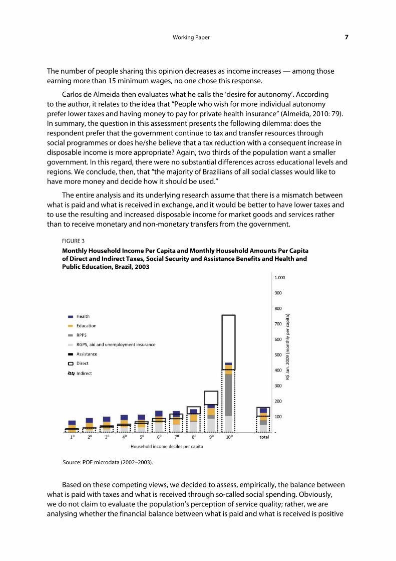
FIGURE 3
Monthly Household Income Per Capita and Monthly Household Amounts Per Capita of Direct and Indirect Taxes, Social Security and Assistance Benefits and Health and Public Education, Brazil, 2003
Source: POF microdata (2002–2003).
Based on these competing views, we decided to assess, empirically, the balance between what is paid with taxes and what is received through so-called social spending. Obviously, we do not claim to evaluate the population’s perception of service quality; rather, we are analysing whether the financial balance between what is paid and what is received is positive
8 International Policy Centre for Inclusive Growth
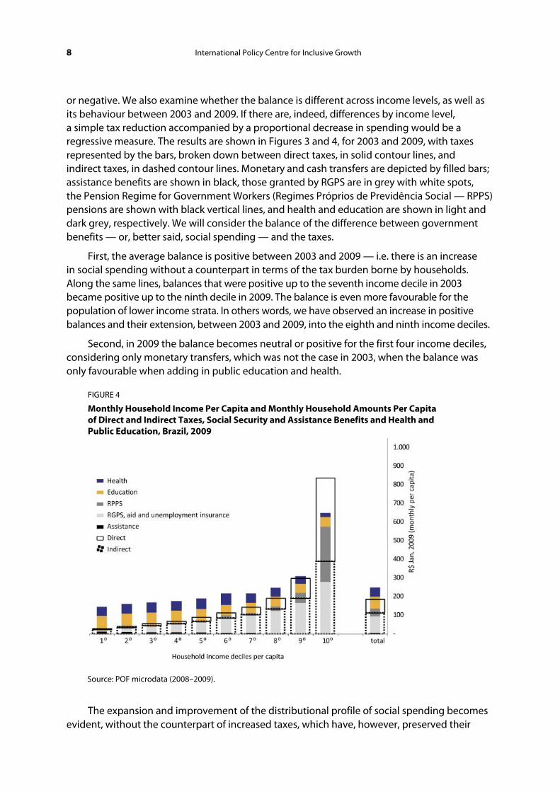
or negative. We also examine whether the balance is different across income levels, as well as its behaviour between 2003 and 2009. If there are, indeed, differences by income level, a simple tax reduction accompanied by a proportional decrease in spending would be a regressive measure. The results are shown in Figures 3 and 4, for 2003 and 2009, with taxes represented by the bars, broken down between direct taxes, in solid contour lines, and indirect taxes, in dashed contour lines. Monetary and cash transfers are depicted by filled bars; assistance benefits are shown in black, those granted by RGPS are in grey with white spots, the Pension Regime for Government Workers (Regimes Próprios de Previdência Social — RPPS) pensions are shown with black vertical lines, and health and education are shown in light and dark grey, respectively. We will consider the balance of the difference between government benefits — or, better said, social spending — and the taxes.
First, the average balance is positive between 2003 and 2009 — i.e. there is an increase in social spending without a counterpart in terms of the tax burden borne by households. Along the same lines, balances that were positive up to the seventh income decile in 2003 became positive up to the ninth decile in 2009. The balance is even more favourable for the population of lower income strata. In others words, we have observed an increase in positive balances and their extension, between 2003 and 2009, into the eighth and ninth income deciles.
Second, in 2009 the balance becomes neutral or positive for the first four income deciles, considering only monetary transfers, which was not the case in 2003, when the balance was only favourable when adding in public education and health.
FIGURE 4
Monthly Household Income Per Capita and Monthly Household Amounts Per Capita of Direct and Indirect Taxes, Social Security and Assistance Benefits and Health and Public Education, Brazil, 2009
Source: POF microdata (2008–2009).
The expansion and improvement of the distributional profile of social spending becomes evident, without the counterpart of increased taxes, which have, however, preserved their

Working Paper 9
regressive profile. Additionally, the introduction of tax cuts that result in reduced public policies is clearly a regressive measure, given that the balance between what is paid and what is received favours the poorest households.
From the point of view of this paper, the criticism of the tax burden and its regressive nature has become stronger in the political and media spheres, as well as in the technical and academic fields, during the last decade. Examples of increased criticism of the tax burden include:
• the creation, in late 2004, of the Impostômetro (a ‘tax gauge’) by the Brazilian Institute of Tax Planning, in partnership with the Commercial Association of São Paulo;
• the establishment, in 2006 and by the same institute, of the estimated number of working days for the payment of taxes, and the creation, by commercial and business entities, of the ‘Tax-Free Day’ since 2008; and
• publication of the books Simplificando o Brasil (unofficial translation: ‘Simplifying Brazil’), by Fecomércio in 2006, and O Dedo na Ferida: menos imposto, mais consumo by Carlos Alberto de Almeida in 2010.
It is interesting to note that this stronger reaction comes at the same time as a significant decrease in inequality, which largely relates to social spending, rather than to an increase in the tax burden in relation to GDP. As can be seen in Figure 5, the change in the level of the tax burden in relation to GDP occurred between 1998 and 2004. After this period, it showed relative stability.
FIGURE 5
Evolution of the Tax Burden (percentage of GDP) and Gini Coefficient of Household Income Per Capita
Source: Coord. of Public Finances (CFP) of Ipea; PNAD-IBGE.

10 International Policy Centre for Inclusive Growth
Since the growth of the tax burden was so pronounced between 1998 and 20044 and has not worsened in recent years, would these warnings not be rather too late? Figure 5 seems to show that these initiatives, notably Impostômetro and the Tax-Free Day, are relatively mismatched with any growth in the tax burden. It is, however, very contemporary to the downward movement of inequality, which arises largely from the improvement in the spending profile. Some also question whether this attack on the tax burden and its unfair incidence is not really aimed at the progressivity of spending, which has deepened in recent times. This raises the question of whether this attack on the tax burden and its iniquitous effect is really aimed at the progressivity of spending.
Therefore, would the Impostômetro not be a misguided measure, rather than a simple tax meter, since its purpose is not to measure the tax burden but to weaken the funding for social spending that has been growing and becoming more progressive?
2 ESTIMATION PROCEDURES AND DATABASES
The development and improvement of impact estimates of taxation, social security, assistance and public supply of health and education in income distribution largely depend on the quality of the databases. In this section, we present the data used and the procedures developed to assess the distributional effects of taxation and social spending.
The two main information databases used in these estimates are the National Household Sample Survey (Pesquisa Nacional de Amostra de Domicílios — PNAD) and the Household Budget Survey (Pesquisa de Orçamentos Familiares — POF). The PNAD focuses on labour and income data, collecting information on households and individuals. It is conducted annually and uses a significantly large sample. The POF focuses on household spending, generating more ‘accurate’ income information at a higher cost, which implies a lower frequency, as well as a smaller sample and significantly less spatial representation.
The PNAD also offers a rich array of socio-economic and demographic information, among which we highlight incomes from social security and social assistance, school attendance and related characteristics and, in some years, access to and use of health services. In comparison to the POF, however, the PNAD does not cover household spending and does not collect detailed information on income. Thus, the PNAD is deficient with regards to income.
With regards to monetary transfers to households, notably social security and assistance, both studies have questions about receiving these benefits; the POF, however, has more detailed data. Its information about monetary transfers breaks down retirement benefits and pensions, social security and welfare aid — whether public or private — and the various cash transfer and worker support programmes. However, until the last POF in 2008–2009, Brazilian household surveys did not differentiate between the public retirement social security system and the pensions under it.
Regarding taxes, the POF is used, roughly, as the source for estimating tax incidence. This is because, on the one hand, the expenses related to the payment of property taxes — Urban Property Tax (Imposto sobre a Propriedade Predial e Territorial Urbana — IPTU) and Motor Vehicle Tax (Imposto sobre a Propriedade de Veículos Automotores — IPVA) — are collected, and the deductions and collection of income taxes — Individuals’ Income Tax (Imposto de Renda — IR), National Social Security Institute (Instituto Nacional de Seguro Social — INSS) and others — are investigated. On the other hand, spending on goods and services is analysed in great detail, thus allowing the incidence of indirect taxes to be estimated by

Working Paper 11
applying the statutory or effective tax rates. It is, however, possible to estimate the incidence of direct taxes on income through the PNAD, by using the rules for payment of IR and social security contributions.
As for the provision of public goods and services in health and education, the PNAD seems more appropriate, given that access to — and use of — public health is investigated only in special PNAD surveys conducted every five years since 1998. In terms of public education, the two surveys investigate school attendance, its level and grade, and whether it is public or private.
2.1 TAXES
An assessment of the incidence of direct taxes on household income can be conducted using both the POF and the PNAD. As mentioned above, POF data on household expenditure contain more precise information on income. Among the expenses are taxes paid, both on assets (property and vehicles) and on income (social security contributions and income tax, among others). Evidently, these are self-declared values, and there may be inaccuracies due to difficulties in recording the amounts paid, due to the under-declaration of income and assets, as well as the taxes attached to them. It is worth noting that the POF occurs every five years, and only in the last two — 2002–2003 and 2008–2009 — was the coverage national.
Only the POF enables the preparation of incidence estimates vis-à-vis indirect taxes on household income, as it collects data on expenditures on goods and services, the basis for applying legal or effective tax rates levied on consumption. It is assumed, therefore, that the set of indirect taxes applies to consumption, even for taxes with incidence based on income or corporate revenue.
In any case, PNAD data can be used to estimate the incidence of direct taxes, specifically those levied on income and real estate — specifically, IRPF, social security contributions and IPTU. These estimates are made by applying the legal norms relating to these taxes to the information in the PNAD on income received, labour relations (type of occupation) and the declared values for properties, to obtain potential amounts for IRPF, social security contributions and taxes.
Using the POF, the evaluation of the distributional impact of taxation covers about 60 per cent of the national tax burden. This level of coverage is quite impressive, considering that about 30 per cent of the taxes not covered refer to the corporate revenue tax (Imposto de Renda de Pessoa Jurídica — IRPJ), the portion of employers participating in social security contributions and other taxes that affect corporations or employers. The remainder includes certain taxes that, although important, do not affect the income and/or assets of households, or are difficult to handle, such as the financial transaction taxes (Contribuição Provisória sobre a Movimentação ou Transmissão de Valores e de Créditos e Direitos de Natureza Financeira — CPMF — and Imposto sobre Operações Financeiras — IOF) and taxes on the transfer of property which, together, account for 5.4 per cent of the national tax burden. After removing the CPMF, the importance of this group has decreased significantly.
2.1.1 Direct Taxation
The POF investigates various taxes levied on earnings, and differentiates between social security contributions (or public welfare), income tax and other deductions5 that affect labour income — both primary and secondary. For other income, including retirement and other pensions, income transfer programmes, aid, scholarships, alimony, donations and rents, the

12 International Policy Centre for Inclusive Growth
total deductions are investigated, without any differentiation. This also occurs in the case of other earnings, including the 13th month of salary and holiday allowances, withdrawal of Contribuição para os Programas de Integração Social e de Formulação do Patrimônio do Servidor Público (PIS/Pasep) and FGTS, workers’ severance, sales, profits, loans, inheritances and dividends, for which the information refers only to the total deductions.
The way information is presented, we can conclude that, under ‘other deductions’ in labour income, ISS6 and a group of other taxes on income are included in the calculation. As for the ‘deductions’ from income coming from sources other than labour, and the ‘deductions’ from other earnings, figures for pensions, IR and ISS contributions are included, in addition to other deductions that do not relate to tax charges.
TABLE 1
Groups of Taxes with their Descriptions in POFs (2002–2003 and 2008–2009)
Group of taxes
Type of tax Description within POF
INSS
Social security
contributions on labour
income
Deduction from labour income (private‐sector employees, public‐sector
employees, domestic workers, temporary employees in rural areas, employers
and self‐made income) for public welfare
Individual INSS
contributions
Public welfare, Funrural; collective work insurance (public welfare pension);
special fund for the military police (military pension); state‐level social security;
municipal‐level social security; military pension, federal pension, military pension
fund; public pension
INSS of domestic workers Spending related to contributions to domestic workers’ pension
IR
(Income Tax)
Income tax on labour
income
IR deduction from labour income (private‐sector employees, public‐sector
employees, domestic workers, temporary employees in rural areas, employers
and self‐made income)
Individual spending on
income tax Complement to the income tax; income tax from the previous year
IPVA IPVA and fees for cars and
other vehicles
Licence plate, Licensing, fines, IPVA, vehicle transfers, documents, driver’s
licences
IPTU
IPTU for the primary
property IPTU and additions, ITR‐IPTR, SPU and Incra IPTU for other properties
Other
Other deductions on labour
income
Other deductions from labour income (private‐sector employees, public‐sector
employees, domestic workers, temporary employees in rural areas, employers
and self‐made income)
Taxes on incomes other
than labour
Deductions from retirement and other pensions, scholarships, alimony, aid,
rents, sales, and salary additions and complements, indemnities, allowances,
13th month of salary and holiday pay
ISS Tax on Services (ISS) (potential)
Professional contributions Professional councils and associations; union contribution, union tax,
cooperative monthly fee and contributions to other associations
Source: IBGE-POF.
In addition to taxes levied on income, the POF also includes taxes on property (IPTU) and on motor vehicles (IPVA). We believe that other taxes levied on vehicles, in addition to IPVA, such as the cost of licensing, licence plates, fines, vehicle transfers, vehicular assessment and drivers’ licences, should be grouped under ‘vehicle taxes’.

Working Paper 13
Taxes on other contributions, professional contributions (unions and professional memberships) or other ‘forms’ of tax incidence described previously — such as the IR relative to the previous fiscal year, any ISS, and social security collections can be extracted from the group that handles expenses related to contributions, transfers and financial burdens. Expenditures referring to the payment of the employee’s portion of social security are reported in home services expenses.
In summary, information in the POF brings together the amounts related to the payment of direct taxes in four groups: IR, IPTU, IPVA and other taxes on income. The latter group includes the two income deduction items — labour and other sources — the potential ISS, professional contributions and CPMF. Table 1 depicts all items considered in the grouping of direct taxes on labour contributions, income tax, IPTU, IPVA and other deductions on income.
2.1.2 Indirect Taxes
Based on the POF, it is possible to estimate the incidence of the following indirect taxes: ICMS, IPI, PIS, the Contribution to Social Security Funding (Contribuição Social para o Financiamento da Seguridade Social — COFINS), ISS and the Contribution to Intervene in the Economic Domain (Contribuição e Intervenção no Domínio Econômico — Cide), using the rates for each of the tax modalities. In the cases of the IPI and ICMS, the rates for each expenditure item, as well as the tax benefits granted to certain products, whether exemptions or reductions on the basis of the calculation, can be obtained from the regulations enforced by the federal government and the states. These benefits are more numerous and more complex in the case of ICMS, and are applied to first-necessity products and goods facing increased competition from other states and/or countries.
In the case of ICMS, one must keep in mind the difficulties in taking into account the effect of granting tax benefits, as they differ between Brazilian states. It is reasonable to assume that those with greater wealth and, therefore, a greater tax base, are more capable of granting tax benefits, particularly on consumption, since this tax is levied, preferably, by the producing state, not the consumer state. There are, therefore, two alternatives in estimating ICMS: we either consider all state laws or we use the rules adopted in one or more than one state — among the most important states — as a reference.
Previous papers that sought to determine the indirect tax burden chose a representative state and, therefore, failed to pick up on the regional differences in tax policy. In this study, we decided to consider the different ICMS rules/regulations of each state. Information pertaining to state and regional tax differences was obtained from the state-level Revenue Services online. ICMS tax rates and exemptions used in the estimation followed the ICMS Regulation (RICMS) of each state and of the Federal District. We applied the rate established by RICMS for each product in each state. We considered the base reductions set forth by RICMS in each unit of the federation — the states and the Federal District. This in itself is quite complex, since the 2002–2003 and 2008–2009 POFs include around 12,000 products or groups of products, levying at least one of the selected indirect taxes on some 9000 products. To make the analysis of the burden in each unit of the federation feasible, we assumed that the rate of the state in which the product is consumed is what applies to the product, regardless of its origin.
In estimating the incidence, certain expenses on which there is no collection of ICMS, IPI or ISS were discarded. In this group we include personal service expenses, the so-called ‘other
14 International Policy Centre for Inclusive Growth
incidental expenses’ and expenses related to reducing one’s liabilities, as well as portions of various expenses and spending on education, health and housing. Furthermore, we consider only monetary expenses, as non-monetary expenses refer to activities conducted at the margins of markets.
In the case of PIS and COFINS, for products subject to taxation in accordance with the law, we used the rate of 9.25 per cent, which applies to companies opting for the non-cumulative tax incidence regime. That is, we consider that these contributions affect household consumption with their rates. It should be noted, moreover, that we considered the special cases of products treated differently in terms of the incidence of this tax. Specifically, we used exemption for vegetables and fruits, as well as specific rates for electricity in each state. And in the case of services, for the purposes of applying the cumulative rate, we considered only one stage of production and marketing, a quite reasonable generalisation for services purchased by households. In this case, the PIS/Pasep rate is 0.65 per cent, and COFINS is set at 3 per cent.
The procedures used to estimate the incidence of these taxes is based, initially, on applying to expenditures (prices) their nominal ICMS rate, thus obtaining the amount corresponding to that tax. It is worth noting that, by applying the nominal ICMS rate to expenses or prices, as stated by the legislation governing this tax, in reality a higher rate is ultimately applied, if we consider that the base of incidence is the price without the tax (ICMS is charged ‘inclusive’). In a second step, we discount the portion corresponding to ICMS from spending, thereby generating new amounts which incorporate the portion corresponding to IPI. From these amounts we extracted the amounts before IPI and ICMS collection, using the following formula:
net expenditures without ICMS and IPI = (expenses -– ICMS) / (1 + nominal IPI rate)
We then obtain the amount of the expenses corresponding to IPI. This sequence of procedures is based on the fact that IPI is part of the basis for calculating ICMS. As for PIS and COFINS, we apply the non-cumulative regime rate and estimate the cumulative regime rate for the sectors grouped in each regime to the overall values of the corresponding expenditures, resulting in the portion relative to these contributions.
When we decide to apply the statutory ICMS and IPI rates to expenses, taking into account exemptions, benefits and methods of operation, we assume that the operation of these taxes is perfect and statutory — without fiscal eliminations, cascading (cumulative) tax collection and tax evasion, among others.
There are two arguments that support this option. The first concerns the fact that the products that take up most of the households’ budgets have, in their supply and marketing chains, a predominance of large industries and businesses that are setting prices, broadly speaking. These are characterised by the legality of their tax and fiscal operations — i.e. tax costs are part of their prices — and the following indirect taxes stand out: ICMS, IPI and PIS/COFINS. This is because the tax share of the prices charged by the major industries, wholesale and retail, is the margin that allows the leaders to become even more competitive. From this stems the second argument. Assuming that these taxes are part of prices in the economy as a whole, they represent a cost for households vis-à-vis the effectiveness of their spending.

Working Paper 15
In the case of Cide levied on fuel transactions (Cide Combustíveis), we consider, on the one hand, the rates set in 2004 (R$0.28 per litre of petrol and R$0.07 per litre of diesel) and, on the other, the average fuel prices in that year. As a result, we arrive at the effective tax rates of 14.7 per cent and 5.6 per cent for petrol and diesel, respectively.
The ISS was also considered in calculating the tax burden, by applying the rates and exemptions in effect in the capitals of each state to the cost of taxable services performed by the households of the respective states. This decision is due to the fact that the POF sample is representative of metropolitan areas, urban regions in the units of the federation and the rural areas of large Brazilian regions.
2.2 SOCIAL SPENDING: CASH TRANSFERS AND PUBLIC PROVISION OF SERVICES
Within the federal government, cash transfers to households, including social security for workers in general (RGPS) and public servants, in addition to substantial portions of social assistance, worker protection and food and nutrition, accounted for just under three quarters of federal social expenditure in 2009. If we consider only public servant and RGPS benefits, the contribution was almost two thirds of the total.
In addition to cash transfers, this study will include estimates of the distributional effects of non-monetary public transfers — i.e. benefits in kind, such as health and education policies. In 2009, spending on public health and education accounted for 11.7 per cent and 6.5 per cent of federal social expenditure, respectively. If we add the expenditures on social security, benefits to civil servants — where retirement and other pensions are paramount — social assistance, employment and defence, the total comes to 92.4 per cent of federal social expenditure. Therefore, the distributional impacts of public spending measured here include almost all of these expenditures at the federal level (Ipea, 2011).
These numbers take on greater prominence when considering the totality of social spending by the federal, state and municipal governments. Between 2005 and 2009, there was a significant growth in the share of social spending out of the total consolidated expenditure of the public sector. Effectively, public-sector expenditure on the policies included here increased from 20.8 per cent of GDP in 2003 to 25.2 per cent in 2009.7
The valuation — monetisation — of public education and health services and their allocations throughout different households according to their socio-economic and demographic characteristics depend on the existence of information on public spending in these two areas and the access and use statistics that apply to these policies. We currently have detailed data on the budgets of different levels of government in these areas, as well as information on the use of these services, according to some of its features, in household investigations.
2.2.1 Social Security and Assistance Benefits: What Information Do We Have About Monetary Transfers?
The social security pension system comprises two public systems — one for private-sector workers and one for civil and military servants — and complementary social security pensions
16 International Policy Centre for Inclusive Growth
managed by private entities and supervised by the public sector. The two public schemes have compulsory membership and are sharing schemes — i.e. the funding collected from taxpayers today are for the payment of benefits provided today.
Data generated by household surveys in Brazil, in the case of the public pension system, did not specify whether the pensions and retirements listed by them referred to the general pension scheme or the pension scheme for civil servants. They did, however, identify earnings originating from private pensions and, in the case of the POF, also the various types of aid, whether granted by employers or by social security. Fortunately, the last POF, for 2008–2009, differentiated between the social security scheme of retirement and other pensions, which was a major advance compared to what was previously delivered.
In the RGPS there are two large sets of benefits: social security and labour accidents. Social security benefits are subdivided into five subsets: retirements, pensions, allowances, aid, maternity pay and the aggregate category ‘other’. Retirement funds are divided by contribution time, age and disability. Aid may be due to sickness, accident and arrest. Accident benefits are divided into three types: aid (sickness, accident and supplemental), pensions for disability and survivor pensions.
It is worth noting that the social security schemes themselves — i.e. for civil servants at the three levels of government, and military personnel — have similar benefits but with higher values and wider inclusion criteria. This can be seen by the existence of childbirth, childcare, health care and education aid in these aid schemes, some of which are unavailable for private-sector workers.
Added to these social security benefits are government cash transfers related to social assistance and worker protection. In the first case, there are the so-called assistance benefits supported by the Social Assistance Law (Lei Orgânica de Assistência Social — LOAS), income transfer programmes for poor households and populations, and social protection programmes for young people and children. Among worker protection schemes, unemployment insurance is the one that comes in the form of a monetary transfer.
Through household declarations, the POF collects information about the receipt of public monetary benefits: pension, assistance, labour and education benefits. These are broken down quite a lot; among social security benefits, it is possible to distinguish, for example, between temporary benefits, such as accident benefits and aid, and permanent benefits — i.e. benefits in the strictest sense of the word — retirement and other pensions.
The POF categories similar to cash transfers made by the government — social security, assistance, worker protection and education benefits — can be grouped into five major clusters: retirement and other pensions; aid; scholarship programmes; cash transfer programmes; and unemployment insurance. This allows the analysis to include some types of optional benefits provided by employers optionally or due to labour agreements, as well as those granted to public servants. Table 2 relates the information contained in POFs to different policies that operate cash transfers.

Working Paper 17
TABLE 2
Types of Cash Transfers (benefits) Investigated in POFs (2002–2003 and 2008–2009) and their Respective Public Policies
Cash transfer category Description within POF Public policy
Retirement and other pensions
Retirements and other pensions from the
National Institute of Social Security and
municipal, state and federal public welfare (1)
and supplements
General Social Security Regime
and Social Security Regimes
(public service): retirement (age,
length of service, disability and
special) and pensions (death)
Continued Cash Benefit (BPC) BPC, LOAS (2) BPC
Aid
Aid for people with disabilities; labour
accidents (public pensions); sickness aid
(3); birth grant; maternity aid; treatment aid
(4); education aid; childcare assistance; school
aid; mother/guardian aid; old age aid;
funeral assistance
RGPS aid (accident or pension
benefits) and benefits for civil
servants
Scholarship Scholarship
Scholarships from agencies
that support research
(CNPq and Capes)
Unemployment insurance Unemployment insurance, unemployment aid
and unemployment assistance Unemployment insurance
Income transfers
Bolsa Família (5); Programme for the
Eradication of Child Labour; School
scholarships (5); minimum income; electric
power aid; Agente Jovem (6), primary food
basket; citizen card (5); milk aid; income grant;
gas assistance and seasonal aid (7)
Bolsa Família, Peti (Programme
for the Eradication of Child
Labour) and Youth Aid from the
Ministry of Social Development;
State and Municipal Income
Transfer Programmes; Social
Electricity Tariff
Source: POF, Cardoso Jr. and Castro (2005), Bulletin of Social Policy IPEA (various issues).
Notes: (1) In the 2002–2003 POF, retirement and other pensions were not differentiated by social security system. (2) In the 2002–2003 POF, BPC was not part of the coded revenues; it may have been assessed as retirement or as old age or disability aid. (3) In 2002–2003, we considered two items of sickness, one of the benefits of social security and the other possibly granted by the employer in the public sector. In 2008–2009, this latter loan was not coded. (4) The treatment aid falls within the aid granted by the employer, in the public sector. (5) Bolsa Família had not yet been implemented when the POF 2002–2003 took place; all the programmes that preceded it were reported. In the 2008–2009 POF, all the codes of these remaining programmes were preserved, since complete unification was only achieved in 2010. (6) In 2002–2003, there was also Adjunto Solidariedade (Solidarity Addition), a programme to support young people, which was replaced by Agente Jovem. (7) Auxílio-Defeso (Off-Season Aid) did not exist when data for the 2002–2003 POF were being collected.

18 International Policy Centre for Inclusive Growth
As mentioned above, the household survey in 2002–2003 did not identify which of the two social security systems it referred to. In the 2008–2009 POF, information was collected on pensions received under the public social security pension system. It was, therefore, necessary to discern the origin of social security benefits within the 2002–2003 POF, and administrative data relating to pension schemes were used for this purpose.
In the case of RGPS and retirees and recipients of federal government pensions, there is information available on the amount of benefits paid monthly, broken down by compatible value ranges.8 For retirees and state and municipal government pension recipients, administrative records (from MPS and STN/MF) only provide annual expenditures. Thus, a survey was held on the statements of pension schemes of states and municipalities,9 to establish monthly reference values for state and municipal retirement benefits. Based on this survey, an arbitrary decision was made to set the average monthly earnings in 2003 at R$1800 and R$1000 for states and municipalities, respectively. We then received the estimate of the number of RPPS pensioners and retirees from the states and municipalities, based on the annual amount and estimated average values.
By adding the estimated amount of state and municipal RPPS benefits to the number of RGPS and federal government retirees, we come to R$22.3 million of monthly retirement and pension payments in 2003.10 We used the distribution of retirement amounts by amount ranges pertaining to civil servants retired from the federal executive branch, available in the Ministério do Desenvolvimento Social e Combate à Fome (MDS) Staff Bulletin, as a proxy for all the RPPSs.
2.2.2 Public Provision of Health and Education: Possibilities for Valuation of Non-monetary Benefits
The estimated impacts of so-called ‘public non-monetary benefits’ (non-monetary benefits) — with special emphasis on the supply of educational and health services and goods — depends, on the one hand, on household surveys that assess the use — or, in other words, the ‘consumption’ — of these products and services and, on the other, detailed administrative public spending records. These are broken down by level of government and by different activities and programmes. In the case of the former, it is important to take double counting and omissions into account. The breakdown of programmes is crucial to better identify beneficiaries. It is true that breaking down public spending should be coupled with an assessment of service use, which means that surveys should investigate the use of different services and goods offered by the public sector.
In the case of education, there are estimates for the average annual public expenditure per pupil — broken down by grade levels and by states — developed by the Anísio Teixeira National Institute for Educational Studies and Research (Inep), under the Ministry of Education. However, both household surveys investigate school attendance, whether it is a public or a private school, and the grade and level of education of those attending school. Therefore, the valuation of public education is automatic; Inep’s investment estimates per pupil are applied to people who attend public schools, for each state and educational level.
Spending per student takes into consideration the cost of active personnel, social charges, incidental expenses, capital expenditures and research and development at the three levels of government. As such, it does not include the costs of retirement and other pensions,

Working Paper 19
scholarships, student funding, interest, amortisation and debt charges. Inep releases data on the national average public spending per student, by school levels. These are shown in Table 3, which contains estimated figures for 2000 to 2008, deflated to 2008 amounts. Fortunately, Inep made available the data broken down by state for the period 2003 to 2008.
TABLE 3
Estimated Direct Public Investment in Education per Pupil with the Amounts Adjusted to 2008 Levels by Broad National Consumer Price Index (IPCA) by Level of Education, Brazil, 2000–2008
Grade
Direct public expenditure per student (R$ in 2008)
Total for
all levels
Levels of education
Primary
education
Early
childhood
education
Basic education High
school
Higher
education 1st to 4th grade
early years
5th to 8th grade
final years
2000 1667 1388 1587 1365 1393 1324 15,341
2001 1726 1439 1433 1349 1518 1506 15,161
2002 1722 1426 1350 1576 1463 1060 14,374
2003 1724 1448 1553 1526 1450 1217 12,594
2004 1824 1548 1655 1638 1656 1133 12,749
2005 1940 1643 1566 1833 1746 1146 12,965
2006 2259 1961 1695 2019 2217 1568 13,076
2007 2612 2291 2069 2408 2509 1837 13,861
2008 2995 2632 2206 2761 2946 2122 14,763
Source: Inep/Ministry of Education.
As for health, there are great difficulties involved in collecting data, because household surveys do not include access to and use of health services and goods as part of their basic structures. It is worth underlining that public health care encompasses an extensive range of programmes and activities.
Fortunately, every five years a study is conducted on the health of the population, as a supplement to the PNAD. These studies collect data about, among others, access to — and use of — health services and goods, especially vaccines, medicines, medical and dental appointments, medical tests, outpatient procedures and hospitalisations. Moreover, there are administrative records of expenditures under the Unified Health System (SUS), as well as the costs incurred by the various government levels, organised into the Health Spending System (Sistema de Gastos em Saúde — Siops).
There is also a methodology developed by Ramos (2001) to reconcile sources of information on the use of public health services and administrative records of public spending. The author estimated the distributional impacts of public spending on health by using the PNAD’s health supplement for 1998 and SUS data on outpatient care and hospital admissions. In this study, we used the PNAD health supplements from 2003 and 2008 and outpatient and hospital admission data from Datasus (SIA/SIH) and added other expenses from the Ministry of Health’s financial reports, as well as those incurred by states and municipalities within Siops.

20 International Policy Centre for Inclusive Growth
Based on data from the Ministry of Health’s financial reports in 2003 and 2008, it is possible to classify health expenditures into six major groups and 31 subgroups in 2003 and 30 in 2008, as shown in Table 4. We excluded the Ministry of Health’s expenses for inactive personnel, amortisations, interest and investments, as these costs do not relate to the provision of public health services, at least not at the point in time when the distributional impact is assessed. We can treat them as expenses related to services already rendered, in the case of inactive personnel, or as expenses yet to be incurred, in the case of investments.
TABLE 4
Composition of Public Federal Spending on Health, Brazil, 2003 and 2008
Large group
Subgroup
2003 2008
Hospitalisations
Obstetrics
Paediatrics
Psychiatry
Other hospital admissions
National Cancer Institute (INCA) and social pioneers
Outpatient care
Medical consultations
Dental consultations
Consultations with other professionals
Chemotherapy, haemodialysis and related procedures
Injections and bandages
Outpatient surgery
Cast or immobilisation
Complementary medical tests
Other services
Basic Care Limit (PAB) and Family Health Programme (PSF)
Vaccines and immunisations
Project for the Expansion and Consolidation of Family Health (Proesf)
Other
FNS’s own hospitals
National Agency for Supplementary Health (ANSS)
SUS maintenance (various)
Medication
Basic pharmacy
Low‐income pharmacy
Medication
Sexually transmitted infections/HIV/AIDS
Exceptional medication
Active staff Active staff
Public services
Maintenance of indigenous units
Universal programmes, scientific research
KFW Ceará and Piauí
Prevention of cervical cancer
Source: Ministry of Health financial reports, 2003 and 2008.
Working Paper 21
We group the data into five hospitalisation categories to ensure compatibility between hospitalisation data from the SUS and information from the PNAD and identify the types of hospitalisation people went through in the past 12 months. Children under 11 years of age, women who have had children and people admitted for psychiatric reasons were identified among the total population admitted into hospitals, according to PNAD data. It was then possible to allocate spending on paediatric, obstetric and psychiatric hospitalisations to these subsets of people. Second, we divided the amount spent by the Ministry of Health in these first four subgroups — obstetrics, paediatrics, psychiatry, and other admissions — based on the number of hospitalisations reported within the PNAD. The number of days spent in hospital was also used as a weighting factor. For the aggregate category ‘Inca and social pioneers’, we decided to distribute the amount spent throughout all patients classified as ‘other admissions’.
Regarding outpatient procedures, an effort was made to reconcile the PNAD information regarding such procedures performed in the previous two weeks with the wide range of procedures included in the Outpatient Information System. This compatibility is roughly what Ramos (2001) performed for the 1998 data. However, adjustments were made to accommodate changes in the classification of procedures by SIA/SIH and the addition of new procedures.
For medical and dental consultations, as well as consultations with other health professionals, injections and bandages, outpatient surgery, immobilisations, complementary examinations and other services, we can use a simple average, calculated based on the amount spent and the number of procedures in each category. In allocating expenditures on high-complexity care, we used the category entitled ‘chemotherapy, haemodialysis and related procedures’ from the PNAD health supplement to distribute these costs. Vaccines and vaccinations were distributed equally among the people who claimed to have had this procedure under the SUS.
Total amounts spent on the Basic Care Floor (Piso de Atenção Básica — PAB), the Family Health Programme (Programa Saúde da Família — PSF) and the Programme for Structuring the Family Health Programme (Programa de Estruturação do Programa Saúde da Família — Proesf) were added and allocated equally among individuals who reported having undergone medical consultations, received care from an SUS community agent or other type of health care under the SUS.
The group ‘other’ includes three subgroups: the hospitals themselves, which may be based on information regarding the use of outpatient services or admittances in SUS public hospitals; miscellaneous expenses, especially administrative maintenance, Datasus and aid to public servants, whose amounts can be distributed equally among all who used SUS outpatient services or admissions; and the expenditures of the National Supplementary Health Insurance Agency (Agência Nacional de Saúde Suplementar — ANSS), which can be divided equally among the members of the private sector.
As for medication, the items ‘Basic pharmacy’ and ‘Acquisition and distribution of medication’ were considered a single expense, distributed evenly among people who reported having received free medication. The amounts assigned to ‘Low-income pharmacies’ have been distributed according to the PNAD question regarding prescription drugs received continuously and for free. Since the PNAD does not distinguish between the beneficiaries of drugs to treat sexually transmitted infections and those to treat AIDS, it was decided to distribute the funds spent on them throughout the entire population. Finally, for exceptional drugs, the allocation of expenses was based on the distribution of high-complexity procedures.

22 International Policy Centre for Inclusive Growth
The appropriation of active personnel expenses is tied to labour organisations. Thus, expenditures on active personnel working at Fiocruz, Funasa and ANVISA are of a universal nature and, therefore, distributed among the entire population. In turn, SUS users share equally in expenses related to FNS and individual hospitals. As for ANSS’s active personnel expenses, the total expense was allocated among health plan users. Finally, the last group consists of services that may be considered public goods, whose expenses are divided equally among the target audience.
Since state and municipal spending is not reported in the same way as in the Ministry of Health and SUS, the parameter for allocating these expenses represents the share of federal spending by groups of households, according to per capita household income strata, in selected spatial conglomerates. With regards to state spending, the distribution of federal spending was reproduced in each state. Thus, for example, the total spent by a unit of the federation can be divided among the household strata of that unit, in the same proportions as the federal spending in that state.
In the case of municipalities, two groups were considered: those belonging to metropolitan regions, and others. For the first group, we decided to distribute federal spending in the respective metropolitan areas, so as to distribute the spending of municipalities in the same region. For other municipalities, the option was to add municipal spending in each state (excluding metropolitan municipalities) and distribute these expenditures according to federal spending on outpatient services (excluding highly complex services such as chemotherapy, haemodialysis etc.) in each state.
The decision to use the allocation of federal spending in its entirety, as a parameter of the distribution of state and municipal spending in metropolitan areas, assumes that these administrative levels have the same portfolio of activities as those receiving federal spending. As for the other municipalities, especially small and medium-sized ones, it is assumed that their provision of health goods and services is more limited, which led to us assign their spending on households based on the distribution of federal spending on outpatient procedures.
Since POF data generate better estimates of the distributional impacts of tax and social policies — in this case social security, assistance, employment and educational policies — i t is necessary to ‘attribute’ the results of the distribution of health spending based on PNAD data to the POF.
With these considerations in mind, it was decided to employ a simple method for attributing the health expenditures assessed via the PNAD to the POF. In each of the spatial aggregates common to the two surveys, we calculated the ratio between public spending on health and household income for population strata representing one twentieth of the population, according to household income per capita. Labour income is used because these figures are closer to each other in both surveys, unlike the case of total income.
2.3 INCOME VERSUS SPENDING
For direct taxes to have distributional effects, they must be progressive — i.e. the rates must rise with income — which is the basis of tax incidence. For indirect taxes, the progressivity assessment relies on the association between household income and its consumption profile.

Working Paper 23
For poor households — or those in the lower income strata — consumption expenditures account for almost their entire income. In the richest households, part of the income is saved. As a result, the regressive taxes on consumption are considered the parameter for the ability to pay, rather than consumer spending. There is considerable debate over how to measure the incidence of regressive tax; some advocate spending as the parameter for one’s ability to pay taxes on consumption, while others believe that income should be kept as the parameter.
The argument for choosing consumer spending as the basis for analysing the incidence of indirect taxation is because it more adequately reflects the standard of living of households than income, since they are more stable throughout a person’s life cycle. This stability is founded on the assumption that consumers level out these expenditures over time, using them for savings or for incurring debt, thus avoiding income variations. The result is that spending is more suitable as a parameter of the ability to pay, because it better reflects what we call ‘permanent income’ — i.e. long-term consumption opportunities.
There are two types of criticism against the use of spending as a parameter to measure the progressivity or regressivity of taxation. The first one, more theoretical and presented earlier, is that using it inhibits redistributive objectives built into tax systems. For taxation to have distributional effects, one must use income, which is the variable that best represents wealth. As Vianna (2000: 62) states: “[...] The idea of preserving savings — implicit in the approach of using consumption as a parameter for the incidence of indirect taxation — loses meaning or becomes ill-suited, since the decision to save necessarily implies the accumulation of wealth.”
There are also empirical objections to the use of spending. The first relates to difficulties in defining what should be excluded from the calculation of overall spending to reach a figure for consumer spending that is, effectively, characterised by stability over time. For instance, in addition to spending on taxes and the spending intended to increase assets and reduce liabilities, should we also disregard expenses related to the purchase of durable goods, maintenance of one’s home and other less frequent expenses? Another objection states that, in most studies on inequality, the inequality measures are income-based as well as poverty and extreme poverty estimates.
This objection is even greater when direct taxation is brought into the scope of the assessment, effectively levied on income, and government cash benefits, the provision of which is related to income — or, rather, to labour and/or insufficient income.
In this discussion about which parameter to use to assess tax incidence, it is important to point out that the POF regularly reports budgetary deficits in households located in the lower and medium income strata. In other words, the income reported by these households is lower than the overall disbursement. For those households located at the lower end of the distribution, such a mismatch can also be observed in consumer spending. This situation, which is not observed in higher-income households, is dually reflected in the discussion of which parameter should be used when evaluating the incidence of taxes and inequality: a) regressivity is obvious — and can even be quite pronounced — when using income as a measure of evaluation; and b) inequality in the spending distribution is lower than in the income distribution.
24 International Policy Centre for Inclusive Growth
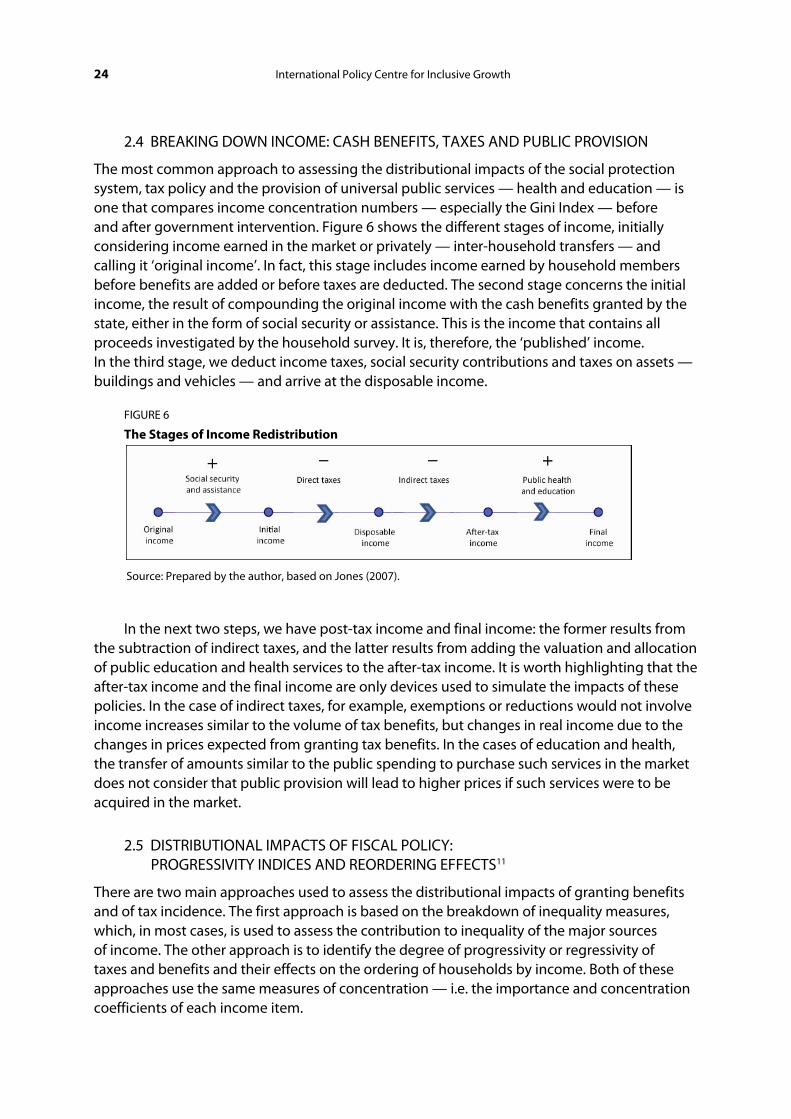
2.4 BREAKING DOWN INCOME: CASH BENEFITS, TAXES AND PUBLIC PROVISION
The most common approach to assessing the distributional impacts of the social protection system, tax policy and the provision of universal public services — health and education — is one that compares income concentration numbers — especially the Gini Index — before and after government intervention. Figure 6 shows the different stages of income, initially considering income earned in the market or privately — inter-household transfers — and calling it ‘original income’. In fact, this stage includes income earned by household members before benefits are added or before taxes are deducted. The second stage concerns the initial income, the result of compounding the original income with the cash benefits granted by the state, either in the form of social security or assistance. This is the income that contains all proceeds investigated by the household survey. It is, therefore, the ‘published’ income. In the third stage, we deduct income taxes, social security contributions and taxes on assets — buildings and vehicles — and arrive at the disposable income.
FIGURE 6
The Stages of Income Redistribution
Source: Prepared by the author, based on Jones (2007).
In the next two steps, we have post-tax income and final income: the former results from the subtraction of indirect taxes, and the latter results from adding the valuation and allocation of public education and health services to the after-tax income. It is worth highlighting that the after-tax income and the final income are only devices used to simulate the impacts of these policies. In the case of indirect taxes, for example, exemptions or reductions would not involve income increases similar to the volume of tax benefits, but changes in real income due to the changes in prices expected from granting tax benefits. In the cases of education and health, the transfer of amounts similar to the public spending to purchase such services in the market does not consider that public provision will lead to higher prices if such services were to be acquired in the market.
2.5 DISTRIBUTIONAL IMPACTS OF FISCAL POLICY: PROGRESSIVITY INDICES AND REORDERING EFFECTS11
There are two main approaches used to assess the distributional impacts of granting benefits and of tax incidence. The first approach is based on the breakdown of inequality measures, which, in most cases, is used to assess the contribution to inequality of the major sources of income. The other approach is to identify the degree of progressivity or regressivity of taxes and benefits and their effects on the ordering of households by income. Both of these approaches use the same measures of concentration — i.e. the importance and concentration coefficients of each income item.

Working Paper 25
The assessment of effects based on ex post income emphasises the evaluation of possible changes in social security, assistance, benefit and tax policies, based on the prevailing situation.
Let us consider that income ix — after the benefit or tax or, more broadly, ex post income — is arranged so that:12
nxxx ≤≤≤ K21
The Gini Coefficient of this distribution can be calculated by:
),cov(2ix xi
nG
μ= , with i
n
ix
n 1
1=∑=μ (1)
It is assumed that the income ix consists of k segments:
hi
k
hi xx
1=∑= (2)
The average of the hth segment is:
hi
n
ih x
n 1
1=∑=μ (3)
and its share in total income is;
i
n
i
hi
n
ihh
x
x
1
1
=
=
∑
∑==
μμ
ϕ (4)
Substituting (2) into (1), one gets:
),cov(1 21
hih
h
k
hx xi
nG
μϕ
=∑= (5)
Similarly to (1), one can define the concentration ratio of the hth segment as:
⎟⎟⎠
⎞⎜⎜⎝
⎛==
h
hihi
hh
xin
xin
Cμμ
, cov2),cov(2 (6)

26 International Policy Centre for Inclusive Growth
It should be kept in mind that the concentration ratios are defined based on sorting by final income. As a result of (5) and (6), it follows that:
hh
k
hx CG ϕ
1=∑= (7)
As can be seen, the concentration ratio is proportional to the covariance between the i positions and the relative incomes hhix μ . Thus, the concentration ratio is not affected by the sign change in this part, since all relative incomes will remain the same.
2.5.1 The Kakwani Progressivity Index13
If zi is the initial income, and ti is the tax, the average tax rate is:
z
t
i
n
i
i
n
i
z
tg
μμ
=∑
∑=
=
=
1
1 , (8)
wherein zμ is the average initial income, and tμ is the average tax.
In this item, we assume that people are ordered according to initial income amounts — i.e.:
nzzz ≤≤≤ K21
Then the Gini Index of the ex ante income is:
),cov(2i
zz zi
nG
μ=
and the concentration ratio of the tax is:
),cov(2i
tt ti
nC
μ=
If tzC − is the income concentration ratio after tax collection, and tzG − is the respective Gini Index, the Kakwani Progressivity Index is defined as:
ztK GC −=Π (9)

Working Paper 27
and it can be shown that:
)(1 tztzKtzz CG
ggGG −−− −−−
=− Π (10)
If the tax does not cause a reordering of incomes, we have tztz CG −− = — a change in the Gini Index in which )( tzz GG −− is proportional to the index of progressivity KΠ . Logically, the effect on inequality will rise at the same pace as the average rate g. In the more general case, as shown in expression (12), there may be an effect of reordering that will never be positive, since
tztz CG −− ≥ (the Gini Index of a distribution may not be lower than the concentration ratio for an order different from that of the variable itself).
Consider, then, that the ex post income is obtained by adding a benefit ( ib ) to the initial income ( iz ). We have:
z
b
i
n
i
i
n
i
z
b
μμβ =
∑
∑=
=
=
1
1, (11)
with bμ as the average value of the benefit. Using the order according to increasing initial income amounts, the benefit’s concentration ratio is:
),cov(2i
bb bi
nC
μ= .
If bzC + is the income concentration ratio after the benefit, and bzG + is the respective Gini Index, the Kakwani Progressivity Index is defined as:14
bzK CG −=ρ (12)
and it can be shown that the change in the Gini Index due to the benefit is:
)(1 bzbzKbzz CGGG +++ −−+
=− ρβ
β (13)
The expressions (10) and (13) show that the change in inequality stems from the progressivity of the tax or benefit, weighted by its participation in later income15 and changes in household ordering. The second term in the 2nd item of expressions (10) and (13) is always

28 International Policy Centre for Inclusive Growth
negative, indicating that, in the assessment of distributional impacts based on previous income, the reordering effects can cause a reduction in the measure of progressivity.
2.5.2 Progressiveness and Reordering: Assessment Based on Ex post Ordering
From the above, it is evident that the assessment of the effects of benefits or tax incidence on inequality depends on which definition of income is used to order the households. The main reason is that the order changes according to the income used as the basis for the assessment.16
We must start with expressions17 to achieve the goal of understanding what determines inequality in income subsequent to benefits or tax incidence: initial )( bz + , final )( dbz −+ and disposable
)( tbz −+ bzG + , dbzG −+ , tbzG −+ , which means prioritising the ordering according to income amounts after government intervention.
It follows that:
)()( bzbztbzttbzbz CGGCgGG ++−+−++ −+−=− , (14)18
and that the concentration ratios are calculated based on ordering by disposable income.
It was decided to use )( tbzt GC −+− as the Lerman and Yitzhaki Progressivity Index for LYΠtaxes, since these authors question the analysis based on the ordering by ex ante income, supporting the use ordering by ex post income.19
It follows, then, that:
)( bzbzLYtbzbz CGgGG ++−++ −+=− Π (15)
This expression shows that, similarly to what was shown in the previous example, the change in the Gini Index is composed of a term associated with a measure of tax progressivity and a pure reordering effect.
Similarly to taxes, the interpretation of income inequality subsequent to the granting of the benefit )( bz + should be based on the ordering according to the values of bz+ . The concentration ratios refer to the ordering of bz+ .
It follows that:
)()( zzbbzbzz CGCGGC −+−=− ++ β (16)
The Lerman and Yitzhaki Progressivity Index for benefits is defined as:
bbzLY CG −= +ρ

Working Paper 29
Substituting into (18), it follows that:
)( zzLYbzz CGGG −+=− + βρ (17)
This expression shows, once again, how the change in the Gini Index stems from a progressivity measure and reordering effects.
“In the case of tax-induced changes in Ginis, the first term in equation [14 and 17] is greater, equal, or smaller than zero depending on whether the tax, on average, is progressive, a constant share of income, or regressive. […] The major difference between this index and Kakwani’s measure of progressivity is that Kakwani weights the income changes by before-tax rankings, while the progressivity index implied in equation 4 [16] weights by after-tax rankings” (Lerman and Yitzhaki, 1995: 51).
3 TAX INCIDENCE, GRANTING OF SOCIAL SECURITY, ASSISTANCE AND BENEFITS, AND USE OF PUBLIC SERVICES IN EDUCATION AND HEALTH
3.1 INCIDENCE OF DIRECT TAXATION
What do the studies based on the POF show us? Estimates by Vianna (2000) for 1995–1996, Silveira (2008) for 2002–2003 and the ones reported here, for 2002–2003 and 2008–2009, show a low level of progressivity of direct taxation in the country. In 1995–1996, while direct taxes collected from households with household incomes greater than 30 times the minimum wage were six times greater than those collected from families with incomes of up to two minimum wages, the income of the former group was 37 times the income perceived by the poorest groups. Thus, as pointed out by Vianna et al. (2000: 49), using as a “benchmark for comparing the progressivity of a tax system [...] the differences observed in the distribution of income across families and individuals, the evidence found suggests that the degree of progressivity of direct taxation is insufficient to offset the high degree of income inequality in Brazilian society.”
As for the 2002–2003 and 2008–2009 POFs, households located in the poorest decile of the population allocated, respectively, 3.7 per cent and 3.0 per cent of their income to the payment and/or collection of direct taxes, while for the richest decile, the tax burdens were 12.0 per cent and 13.0 per cent, respectively. The average per capita household income of the poorest 10 per cent represented 1.1 per cent and 1.6 per cent of the income of the richest decile, in 2003 and 2009, respectively.
No major changes were found in the progressivity of direct taxation between these two POFs, given that the profile of the incidence of direct taxes, by income level, has not particularly changed. In fact, there was a small increase in the direct tax burden on households, which is distributed in a similar way to the previous incidence.
In Figure 7 we see that the progressivity in direct taxation is due, notably, to the incidence of income tax, and that taxes on assets have a profile that is, roughly, neutral. With regard to social security contributions, the reduced progressivity observed can be attributed to the low
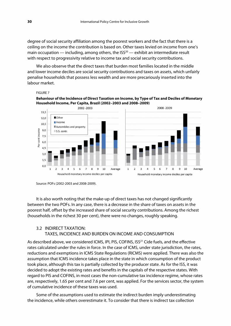
30 International Policy Centre for Inclusive Growth
degree of social security affiliation among the poorest workers and the fact that there is a ceiling on the income the contribution is based on. Other taxes levied on income from one’s main occupation — including, among others, the ISS20 — exhibit an intermediate result with respect to progressivity relative to income tax and social security contributions.
We also observe that the direct taxes that burden most families located in the middle and lower income deciles are social security contributions and taxes on assets, which unfairly penalise households that possess less wealth and are more precariously inserted into the labour market.
FIGURE 7
Behaviour of the Incidence of Direct Taxation on Income, by Type of Tax and Deciles of Monetary Household Income, Per Capita, Brazil (2002–2003 and 2008–2009)
Source: POFs (2002-2003 and 2008-2009).
It is also worth noting that the make-up of direct taxes has not changed significantly between the two POFs. In any case, there is a decrease in the share of taxes on assets in the poorest half, offset by the increased share of social security contributions. Among the richest (households in the richest 30 per cent), there were no changes, roughly speaking.
3.2 INDIRECT TAXATION: TAXES, INCIDENCE AND BURDEN ON INCOME AND CONSUMPTION
As described above, we considered ICMS, IPI, PIS, COFINS, ISS21 Cide fuels, and the effective rates calculated under the rules in force. In the case of ICMS, under state jurisdiction, the rates, reductions and exemptions in ICMS State Regulations (RICMS) were applied. There was also the assumption that ICMS incidence takes place in the state in which consumption of the product took place, although this tax is partially collected by the producer state. As for the ISS, it was decided to adopt the existing rates and benefits in the capitals of the respective states. With regard to PIS and COFINS, in most cases the non-cumulative tax incidence regime, whose rates are, respectively, 1.65 per cent and 7.6 per cent, was applied. For the services sector, the system of cumulative incidence of these taxes was used.
Some of the assumptions used to estimate the indirect burden imply underestimating the incidence, while others overestimate it. To consider that there is indirect tax collection

Working Paper 31
on all expenditures on products and services investigated by the POF means disregarding the existence of tax avoidance and evasion and the efficiency of the tax collection system. The assumption that indirect taxes on added value ‘work’ perfectly — i.e. there are no cascading charges, either due to the discontinuity of collection and credits or due to the interpretation of the exemption rules — results in the underestimation of the incidence of these taxes.
Figure 8 presents the results of the estimation of the incidence of indirect taxes on the total household income in 2009 and 2003, according to income levels. Two facts are noteworthy: first, the high regressivity of indirect taxes, particularly ICMS and PIS/COFINS; second, the stability observed in the indirect burden on households, especially in the first income decile. In reality, there were small reductions in the share of indirect taxes on income, between 1 and 2 per cent, with an emphasis on the drop that occurs in the 2nd, 3rd and 4th deciles. This maintains the highly regressive profile of the incidence of indirect taxation.
FIGURE 8
Behaviour of the Incidence of Indirect Taxes on Total Income, by Type of Tax and According to Per Capita Household Final Monetary Income Deciles (net of taxes), Brazil (2002–2003 and 2008–2009)
Source: POF (2002–2003 and 2008–2009) microdata.
No significant differences were found in the make-up of indirect taxation in the different income deciles. The ICMS is predominant, and accounts for about 50 per cent of the indirect burden assessed; PIS/COFINS comes in second, with a share of around 30 per cent. IPI, ISS and Cide-fuels saw their shares increase as the level of income rose, a behaviour more widely seen in 2002–2003. This closer approximation of the composition of indirect taxes of different income strata is due to improved income distribution and to the convergence of consumer baskets, with a growth in the share of spending in poor households with the purchase of industrial products and services in general.

32 International Policy Centre for Inclusive Growth
Progressivity indicators of indirect taxes were stable between 2003 and 2009; there was a significant decrease in their share of income. This was reflected in a significant change in the marginal contribution of indirect taxes to inequality — i.e. a small increment in indirect taxation came to have a smaller concentration effect.
3.3 THE TOTAL TAX BURDEN
Table 5, which shows the estimated direct and indirect tax burdens on families in 2009, shows that the high degree of regressivity in indirect taxation is not offset by the progressivity of direct taxes, resulting in an overall regressivity of the tax system. This occurs when we use incomes as the basis for assessing the burden; it is even more regressive when considering only the monetary portion of income. The situation is quite different when using spending as the parameter of incidence. Even so, indirect taxes show regressivity, albeit not as significantly, as they accounted for almost one fifth of the money spent in the lower deciles, each falling slightly in the higher income deciles, reaching 14 per cent among the richest decile.
When calculating the incidence of tax, in the case of indirect taxes, we use monetary spending and monetary income; in the case of direct taxes, we conclude that the taxes are ‘neutral’ — i.e. the incidence is similar in the various income levels. It is around 26 per cent of the monetary spending and income mix.
However, as previously discussed, the best parameter for assessing the tax burden is income. There is, however, the drawback of using monetary income, given that low-income families, and even those in average distribution deciles, have significant budget deficits. And, since the calculation of indirect taxation is done based on monetary expenses, the share of indirect taxation in the monetary income of poor households is very high — or, rather, barely believable. For this reason, we used the total income as the basis for calculating the tax burden on households.
TABLE 5
Share of Direct and Indirect Taxes on Income and Expenditure, Brazil (2008–2009)
Available
income
deciles
Indirect (%) Direct (%) (1) Total taxes (5)
Total
income
Monetary
income
Total
expenditure
Monetary
expenditure
Total
income
Monetary
income
Total
income
Monetary
income
Mix spending
(indirect) and
income (direct) (2)
Total Monetary
1st 28 47 16 21 4 6 32 53 20 27
2nd 22 30 16 21 4 5 25 35 20 26
3rd 19 25 16 20 4 6 23 31 20 26
4th 18 23 16 20 5 6 23 29 21 26
5th 17 21 16 20 5 6 22 27 21 26
6th 16 19 16 19 5 7 22 26 21 26
7th 15 18 15 18 6 7 21 25 21 25
8th 15 17 15 18 7 8 21 25 22 26
9th 13 15 14 17 8 9 21 24 23 26
10th 10 10 12 14 11 12 21 23 23 26
Total 13 15 14 17 8 10 22 25 23 26
Source: POF microdata (2008–2009).

Working Paper 33
According to Silveira (2003), the burden of indirect taxes on metropolitan household incomes in 1995–1996 was 25.7 per cent in the first decile, 14.3 per cent in the fourth decile, 10.5 per cent in the seventh decile and only 6.5 per cent in the highest decile. When we add the incidence of direct taxes, the total tax burden on household income reaches 28 per cent in the first decile, 23 per cent in the second, and 20 per cent in the third, fourth and fifth deciles. In the richer half, the figure is 14–16 per cent.
The burden of direct taxes on the monetary income of households in 2002–2003, according to Silveira (2008), was between 3 per cent and 5 per cent in the first five income deciles, rising to almost 8 per cent in the eighth decile and 12 per cent in the richest decile. Progressivity remains insufficient to counter the regressive indirect taxes, whose incidence on monetary income exceeded 30 per cent in the poorest half of the population, compared to 19 per cent in the eighth and 12 per cent in the tenth deciles. Thus, the tax burden on the monetary income of the poorest households was more than twice the figure observed in the higher income deciles.
Figure 9 compares the results of the distribution of the total tax burden across households in 2008–2009 and that observed in 2002–2003, based on total income, because, as has been suggested, this has proven to be the best parameter to evaluate the tax burden. As stated above, the use of total income aims to alleviate the budget deficit problem, to provide more consistent results regarding the incidence of indirect taxes in the first few income deciles. In the case of indirect taxes, the assessment was based on disposable income — i.e. net of direct taxes. Thus, Figure 9 shows the shares of direct and indirect taxes on total initial income, as well as the share of indirect taxes in the total disposable income — net of all direct taxes.
Again, the regressivity of indirect taxation and progressivity of direct taxation are shown, resulting in a total tax burden that is regressive: among the poorest decile, it reaches around 32 per cent, and then it falls steadily to 12 per cent among the richest decile. As already mentioned, the changes between 2003 and 2009 are negligible. On the one hand, we see a slight decrease in the incidence of indirect taxation, between 1 and 2 per cent; on the other hand, there was also a marginal increase of 0.5 per cent in direct taxation. Therefore, the total tax burden on families and their distributional profile changed very little.
FIGURE 9
Tax Burden on Total Income, Brazil (2002–2003 and 2008–2009)
Source: POF (2002–2003 and 2008–2009) microdata.

34 International Policy Centre for Inclusive Growth
The regressivity of indirect taxation is once again illustrated when evaluating the ratio between the incomes of the richest and the poorest, compared to the value of this ratio for indirect taxes. Indeed, while the average total income of the richest 20 per cent is 5.6 times greater than that of the poorest 40 per cent, their indirect tax burden is only about three times the size. This situation is even more acute when we compare the richest 10 per cent and the poorest 10 per cent: total income is 29 times greater, while the indirect tax burden is just 10 times greater.
Importantly, the differences between the 2009 and 2003 estimates — with respect to the share of direct and indirect taxes on income and spending — focus on the incidence of indirect taxes on monetary income. For the rest, variations are marginal. Indeed, between 2009 and 2003 there was a significant drop in the incidence of indirect taxes on monetary income, greater than or equal to 5 per cent in the first three income deciles and lower in higher income strata. Could there have been such a significant decrease in the indirect tax burden and its regressivity? There are no facts that support this behaviour, as there have not been significant changes in the rates and rules of operation of the main indirect taxes.
What actually happened was a substantial improvement in the budget balance of the poorest households, due to their significant income growth and their use of formal credit. The weight of indirect taxes on monetary income in 2002–2003 was calculated in the papers by Zockun (2005), Fecomércio (2006), Afonso (2010) and the Ipea Presidential Communiqué (Ipea, 2009). It received widespread attention by pointing to indirect tax burdens of 50 per cent among the poorest households. This can also observed in this study, when using monetary income as the incidence parameter (see Table 5).
However, as mentioned above, the use of monetary income overestimates the weight of taxation on low-income households, by ignoring the substantial budget deficits reported for these households by the different POFs. To illustrate the effects of lowering the budget deficits of households in the middle and lower income deciles, we estimated what would be the share of indirect taxes in monetary income if the relationship to monetary spending were preserved — i.e. if we considered the same budget deficit in 2003 for 2009. Figure 10 illustrates the result of this counterfactual exercise. It is clear that the burden of indirect taxes and their regressivity would remain roughly the same in 2009.
FIGURE 10
Incidence of Indirect Taxes on Monetary Income, by Income Deciles, Brazil (2002–2003 and 2008–2009)
Source: POF (2002–2003 and 2008–2009) microdata.

Working Paper 35
3.4 SOCIAL SECURITY AND ASSISTANCE: INCOME SHARE AND DISTRIBUTION STRUCTURE
The distributional profile of social security can be evaluated based on the data from the POFs, by comparing the composition of social security contributions of workers and retirement and other pensions by income strata, as shown in Table 6.
Considering that social security in Brazil — either RGPS or RPPS — is a sharing-based system (i.e. today’s assets fund the benefits of people who are currently inactive), it is valid to measure the shares of contributions and benefits that apply to the different income groups. However, this raises questions about the income share of contributions and retirement pensions, of 3.3 per cent and 17.1 per cent, respectively, in 2009: What kind of sharing system is this, with such a degree of actuarial imbalance? First, it should be noted that the contributions paid by employers were not considered; these are roughly twice those paid by employees. Thus, the contributions would represent 9.9 per cent of income. Furthermore, one must consider that RGPS has a contribution limit, which does not apply to employers. One must also add subsidies to farmers, domestic workers and rural workers, as well as exemptions for small businesses and charities, among others. We then arrive at a better balance between the share of contributions in total personal income and share of retirement pensions in that same income.
TABLE 6
Evolution of Household Income Per Capita and of the Income Share of Retirement Pensions and Social Security Contributions, by Income Decile, Brazil (2003 and 2009)
Deciles of
monetary
household
income per
capita
Percentage share of cash income Monthly monetary household
income per capita
(R$ January 2009) Social security benefits Social security contributions
2002–2003 2008–2009 2002–2003 2008–2009 2002–2003 2008–2009
1 6.8 6.9 1.0 0.7 33.06 54.81
2 15.1 13.6 1.4 1.5 79.38 122.23
3 14.8 14.9 1.9 2.1 125.38 182.38
4 17.7 18.0 2.3 2.4 178.84 248.88
5 13.1 18.1 2.6 2.6 239.93 331.53
6 18.6 24.2 2.7 2.7 319.13 431.11
7 12.0 17.1 3.3 3.1 430.03 563.17
8 11.9 17.7 3.3 3.4 611.28 775.03
9 11.2 17.7 3.6 3.6 981.15 1176.71
10 12.6 16.1 2.9 3.5 2971.71 3443.84
Average 12.8 17.1 3.0 3.3 597.24 733.04
Source: POF (2002–2003 and 2008–2009) microdata.
Between 2003 and 2009, according to the POF, the share of pensions in income increased dramatically, from an average of 12.8 per cent to 17.1 per cent. This increase did not occur in all income groups; it focused on middle and higher income deciles. This is because most beneficiaries of retirement and other pensions are in these income brackets

36 International Policy Centre for Inclusive Growth
Other income transfers have a marginal effect on total income. According to 2008–2009 POF data, aid (whether social security or granted by employers — largely the result of labour agreements), income transfer programmes (the so-called ‘pockets’) and insurance unemployment accounted for 1.0 per cent of cash income. If we add the BPC, the share of assistance income transfers and labour aid amount to 1.4 per cent of initial monetary income. This share is nearly three times higher than the one in the POF from 2002–2003. Even if adjustments are made, seeing as how POF data are undervalued for social security aid and unemployment insurance, these benefits and transfers would reach a maximum of 3.5 per cent of cash income. As for targeting — i.e. the concentration of these benefits in lower income strata — there is a great difference between transfer programmes, on the one hand, and aid and unemployment insurance, on the other. Given that the latter two benefits are only available to workers in the formal labour market, its limited relevance and presence in the lower income strata reflect the precarious labour status of the poorest households and, therefore, the absence of social protection measures for them.
In relation to income transfer programmes (PBF in particular), the data show their importance in the income of the poorest decile, as they represent almost one fifth of monetary income and one tenth of total income, declining progressively as income rises (Figure 10). Seeing as how, between 2009 and 2010, PBF came to encompass about 2 million new households (nearly 13 million households today), it is to be expected that its share in the income of the poorest families has expanded. Data from the 2008–2009 POF show that 80 per cent of the funds transferred via PBF are received by the poorest 40 per cent of households, whose monthly household cash income per capita was R$152.08, in January 2009 values.
FIGURE 11
Share of Bolsa Família, Aid, Unemployment Insurance and BPC in Monetary Income, by Income Deciles, Brazil (2008–2009)
Source: POF (2002–2003 and 2008–2009) microdata.

Working Paper 37
Another way to assess the distributional profile of social security is to compare each income decile’s share of total contributions versus its share of total retirement and other pensions. If they are being distributed similarly, social security would not be enhancing or diminishing the concentration of personal income, roughly speaking. This is the basis for Figure 12, which shows the share of all contributions and retirement and other pensions received by each income decile in both POFs. It also includes the differences between these shares which, as can be seen, vary between 6.0 and 3.4 percentage points.
In this respect, in 2003, the first six deciles received a greater portion of retirement pensions vis-à-vis the total contributions. Of special note is the behaviour of the sixth decile and its near parity with the first. This was offset by a higher share in total contributions than in the retirement pensions of the richest 40 per cent, with special mention of the difference in the ninth decile, which accounts for nearly 20 per cent of the contributions versus a share in total pensions of less than 15 per cent. The richest decile, on the other hand, had a slightly higher share in the set of retirement pensions, compared to its weight in the contribution mix. In 2009, there was a shift toward greater progressivity in social security, since the ‘deficit’ between the shares of the total amount of retirement and other pensions and the total contributions went from the ninth to the tenth decile; it also reduced the mismatches in the remaining deciles.
FIGURE 12
Share of Retirement Pensions (and other pensions) and Social Security Contributions, by Deciles of Household Cash Income Per Capita, Brazil (2002–2003 and 2008–2009)
Source: POF (2002–2003 and 2008–2009) microdata.
It is a fact, however, that there is a large concentration of pension benefits in the wealthiest deciles, with the richest 10 and 20 per cent receiving 44 per cent and 61 per cent, respectively, of the total pension benefits paid in 2009. Although the distribution of contributions is even more concentrated, the distributive gains could be larger.
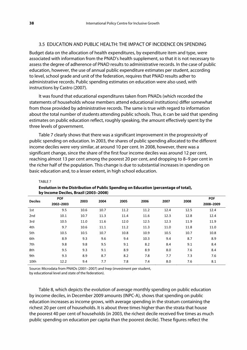
38 International Policy Centre for Inclusive Growth
3.5 EDUCATION AND PUBLIC HEALTH: THE IMPACT OF INCIDENCE ON SPENDING
Budget data on the allocation of health expenditures, by expenditure item and type, were associated with information from the PNAD’s health supplement, so that it is not necessary to assess the degree of adherence of PNAD results to administrative records. In the case of public education, however, the use of annual public expenditure estimates per student, according to level, school grade and unit of the federation, requires that PNAD results adher to administrative records. Public spending estimates on education were also used, with instructions by Castro (2007).
It was found that educational expenditures taken from PNADs (which recorded the statements of households whose members attend educational institutions) differ somewhat from those provided by administrative records. The same is true with regard to information about the total number of students attending public schools. Thus, it can be said that spending estimates on public education reflect, roughly speaking, the amount effectively spent by the three levels of government.
Table 7 clearly shows that there was a significant improvement in the progressivity of public spending on education. In 2003, the shares of public spending allocated to the different income deciles were very similar, at around 10 per cent. In 2008, however, there was a significant change, since the share of the first four income deciles was around 12 per cent, reaching almost 13 per cent among the poorest 20 per cent, and dropping to 8–9 per cent in the richer half of the population. This change is due to substantial increases in spending on basic education and, to a lesser extent, in high school education.
TABLE 7
Evolution in the Distribution of Public Spending on Education (percentage of total), by Income Deciles, Brazil (2003–2008)
Deciles POF
2002–2003 2003 2004 2005 2006 2007 2008
POF
2008–2009
1st 9.5 10.6 10.7 11.2 11.2 12.4 12.5 12.4
2nd 10.1 10.7 11.3 11.4 11.6 12.3 12.8 12.4
3rd 10.5 11.0 11.6 12.0 12.5 12.3 11.9 11.9
4th 9.7 10.6 11.1 11.2 11.3 11.0 11.8 11.0
5th 10.5 10.5 10.7 10.8 10.9 10.5 10.7 10.8
6th 8.9 9.3 9.6 9.4 10.3 9.4 8.7 8.9
7th 9.8 9.8 9.5 9.1 8.2 8.4 9.1 8.4
8th 9.5 9.3 9.1 8.9 8.9 8.0 7.6 8.4
9th 9.3 8.9 8.7 8.2 7.8 7.7 7.3 7.6
10th 12.2 9.4 7.7 7.8 7.4 8.0 7.6 8.1
Source: Microdata from PNADs (2001–2007) and Inep (investment per student, by educational level and state of the federation).
Table 8, which depicts the evolution of average monthly spending on public education by income deciles, in December 2009 amounts (INPC-A), shows that spending on public education increases as income grows, with average spending in the stratum containing the richest 20 per cent of households. It is about three times higher than the strata that house the poorest 40 per cent of households (in 2003, the richest decile received five times as much public spending on education per capita than the poorest decile). These figures reflect the

Working Paper 39
greater number of students from poor households in primary schools, greater access to public universities among children from higher-income families and, furthermore, frequent high school attendance by middle-income families.
The significant increase in spending on primary education and, to a lesser extent, on high school education explains the progressive improvement of spending on education. A consequence of this is the real growth, of around 80 per cent, in spending directed at the poorest 40 per cent of households, compared to an increase of just over 50 per cent in the richest 30 per cent, between 2003 and 2008. As a result, there was a decrease in the ratio between spending on the richest 20 per cent and the poorest 40 per cent, from 3.2 to 2.8, between 2003 and 2008. This also meant a decrease in the concentration ratio of public education.
TABLE 8
Evolution of the Average Monthly Public Spending on Education (pre-school, primary, high school, youth and adult education, technical and higher education), by Income Deciles, Brazil (2003–2007) (R$ December 2009)
Deciles 2003 2004 2005 2006 2007 2008
1 108.77 109.80 118.88 138.68 170.08 191.77
2 118.29 121.00 132.57 154.66 182.21 212.95
3 131.65 134.85 144.79 173.76 199.33 225.91
4 140.18 144.93 156.33 185.40 212.45 247.32
5 152.82 155.95 166.58 200.58 222.29 257.19
6 165.80 168.26 178.13 212.01 239.79 274.73
7 185.93 182.73 194.38 235.78 260.41 299.52
8 212.12 208.90 228.66 272.14 297.79 320.32
9 277.51 276.59 283.35 341.25 371.42 415.95
10 523.72 456.79 516.83 586.43 691.39 801.51
Source: Microdata from PNADs (2001–2007) and Inep (investment per student, by educational level and state of the federation). Deflated by INPC-A; adjusted for the end of year.
Public spending on health proves to be mildly progressive; of note is the behaviour of expenditures on hospitalisations and outpatient procedures. Spending on federal public servants has an incidence profile similar to total spending, and spending on medication boasts a roughly inverted U-shaped distribution. We must observe, however, that the share of spending on medication for the richest decile falls outside this pattern, as it is much smaller than the rest. And, as might be expected, the distribution of expenditures on goods and services considered universal is neutral.
The progressivity of health expenditures is revealed by the fact that the poorest 40 per cent of the population received about half of hospital spending and 45 per cent of the costs of outpatient procedures, compared to 10 per cent for the richest 20 per cent. In the make-up of total expenditures, the poorest half of the population received just over 55 per cent, compared to 20 per cent for the richest 30 per cent.

40 International Policy Centre for Inclusive Growth
TABLE 9
Distribution of Federal Public Spending on Health, According to Expense Items and Income Deciles (percentage of total), Brazil (2008)
Deciles Total Hospitalisations Outpatient
procedures
Universal goods
and services
Federal civil
servants Medication
1st 10.0 12.5 10.5 10.6 11.3 7.6
2nd 11.0 13.0 11.8 9.9 11.7 8.2
3rd 11.3 11.3 12.0 10.0 11.4 12.1
4th 10.7 11.2 11.1 10.1 11.4 8.5
5th 11.3 11.9 11.5 9.9 11.2 10.7
6th 12.7 14.3 12.7 10.0 11.5 15.7
7th 10.5 9.2 10.4 10.0 10.1 10.1
8th 9.6 7.5 9.4 9.9 9.1 11.0
9th 8.4 6.2 7.6 9.8 7.3 11.3
10th 4.7 3.1 3.1 9.8 4.9 4.9
Source: Microdata from PNAD (2008), Datasus and Siops (Ministry of Health).
This distribution of public spending on health is reflected by a concentration coefficient close to zero (i.e. neutral) but with significant distributional impacts, given the degree of income inequality. It is worth stressing that there were no changes in the distributional profile of health spending between 2003 and 2009. Indeed, we observe an actual growth rate that lies above the growth rates of income and consumption.
4 DISTRIBUTIONAL IMPACTS OF TAXES AND SOCIAL SPENDING
4.1 CHANGES IN THE GINI INDEX BY INCOME STAGE
The assessment of the distributional impacts of the social protection system, tax policy and the provision of universal public services — health and education — is one that compares income concentration numbers — especially the Gini Index — before and after government intervention. However, it does not clearly indicate the reason behind the change in the index, whether it was the progressivity of the policy or changes in the household ordering. That is, it does not state which of the two effects was predominant.
The results presented here refer to changes in total income — i.e. including both the monetary and non-monetary portions of income.22 It is worth pointing out that monetary income estimates have a relatively similar behaviour to the behaviour reported here regarding total income. In fact, when considering monetary income, the changes in the Gini Index between the different stages of income are more pronounced.
Figure 13 summarises the evolution of changes in total household monthly income per capita and its inequality (Gini Index) in 2002–2003 and 2008–2009, resulting from policies on social security, assistance, taxes and health and public education. Gains between 2003 and 2009 are clear, both in the amount of social spending and in its distributional effects.
Between 2003 and 2009, there is a clear change in the level of inequality in income distribution, as well as in the amounts. This reduction in inequality occurs in the initial income, since the Gini Index of original income in 2009 is only 2.3 per cent lower than in 2003 but is

Working Paper 41
more than 5 per cent lower for initial income. This difference remains stable at this level (5 per cent) when considering direct and indirect taxes. The gap expands when comparing the final incomes in 2003 and 2009, incorporating education and public health. Specifically in 2009, the Gini Index of final income is 9.3 per cent lower than in 2003, which is almost double the fall in inequality achieved through social security and assistance policies.
The data make it clear that the progress made from 2003 to 2009 is due to public expenditures, not their funding. This is because, as seen before, after the 5.2 per cent drop in the Gini Index for initial monetary income, which includes the granting of social security and assistance benefits, there was no further significant decline in inequality in the stages of income related to tax incidence between 2003 and 2009. The Gini Index of disposable income and after-tax income in 2009 were, respectively, 5.7 per cent and 5.4 per cent lower than the respective indices in 2003. In fact, taxation preserves the same distributional effect, with a 2.5 per cent drop in the disposable income Gini (i.e. after direct taxation), which is more than offset by growth of over 3.5 per cent in the index that reflects the effect of indirect taxes. And, actually, what was more effective in reducing inequality was universal spending — on public health and education.
FIGURE 13
Behaviour of the Gini Index in the Total, Original, Initial, Disposable and Final Income, Brazil (2002–2003 and 2008–2009)
Source: IBGE-POF (2002–2003 and 2008–2009) microdata.
As a result of the greater progressivity of social security and assistance benefits and the stability of the incidence of direct and indirect taxes, there was a more significant drop in the Gini Index between original income and after-tax income. In 2003, the Gini Index fell by only 1.3 per cent as a result of social security, assistance and taxation; it fell by 4.4 per cent in 2009.
Tables 10 and 11 show information about the structure of the distribution of household income per capita, in each of the income stages in 2003 and 2009, respectively. As indicated, there is a significant change between 2003 and 2009 in the decrease in inequality when moving from original income to initial income — the Gini Index decreases by 5.2 per cent in 2009, compared to 2.3 per cent in 2003.

42 International Policy Centre for Inclusive Growth
Between 2003 and 2009, initial and final incomes grew, in real terms, by 20 per cent and 24 per cent, respectively, which, collated with increases of 14 per cent and 21 per cent, respectively, for original and after-tax incomes, shows the growth of public monetary and non-monetary transfers. In 2009, such transfers became more progressive, and, as such, their distributive effects were magnified.
The distributive effects of direct and indirect taxation are very similar, in relative terms, between the two POFs. What differs is that, in 2003, the decline in inequality arising from the granting of social security and assistance benefits and the payment of direct taxes was almost completely nullified by the incidence of indirect taxes. This situation was not seen in 2009, when the regressive effect of indirect taxation was insufficient to compensate for the inequality before the granting of social security and assistance benefits and payment of direct taxes. However, the percentage increases in the Gini Index between disposable and after-tax incomes are fairly close — 2.1 per cent in 2003 and 3.5 per cent in 2009 — because the fall in the Gini Index resulting from cash transfers in 2009 was quite significant, reducing the backflow triggered by the indirect taxes.
TABLE 10
Distribution of Total Household Income Per Capita for the Different Income Stages, According to Income Quintiles, Brazil (2002–2003)
Share of income for each quintile and decile (%) Original
income
Initial
income
Disposable
income
Income after
taxation
Final
income
Quintiles 1st 2.2 2.6 2.7 2.5 4.1 2nd 5.4 5.8 6.1 5.9 7.7 3rd 9.9 10.1 10.5 10.4 11.7 4th 18.0 17.9 18.4 18.8 18.6 5th 64.5 63.5 62.3 62.5 58.0 Gini Coefficient (%) 60.5 59.1 57.9 59.7 52.8 Average (R$ in January 2009) 616.16 697.75 642.92 544.51 17.65
Source: IBGE/POF (2002–2003) microdata.
TABLE 11
Distribution of Total Household Income Per Capita for the Different Income Stages, According to Income Quintiles, Brazil (2008–2009)
Share of income for each quintile and decile (%)
Original
income
Initial
income
Disposable
income
Income after
taxation Final
income
Quintiles 1st 2.2 3.0 3.2 2.8 5.1 2nd 5.8 6.6 6.9 6.5 8.8 3rd 10.4 11.0 11.5 11.1 12.6 4th 18.6 18.8 19.3 18.9 19.0 5th 63.0 60.6 59.2 60.6 54.5 Gini Coefficient (%) 59.1 56.0 54.6 56.5 47.9 Average (R$ in January 2009) 703.79 840.34 769.32 661.19 69.22
Source: IBGE/POF (2002–2003) microdata.

Working Paper 43
Finally, the public provision of social services also proved much more effective in distributional terms, causing a decrease in the Gini Index of 17 per cent, compared to just over 13 per cent in 2003. Specifically, in 2003, the Gini fell from 0.597 to 0.528 as a result of the usage profile of public education and health provision, an amount well below the Gini of the other income stages. In 2009, public provision caused a decrease in the Gini Coefficient of total income, from 0.565 to 0.479 — i.e. it was taken to a level below 0.50. The expansion of the redistributive potential of public provision is reflected in a greater decrease in the Gini Index when moving from after-tax income to final income, from 11.6 per cent in 2003 to 15.2 per cent in 2009.
In short, there was, on the one hand, an increase in the distributive gains from social security and assistance, as well as public health and education, and, on the other, the regressive impacts of taxation were roughly preserved, due to the small weight of direct taxes and the regressivity of indirect taxes. It is interesting to note that the percentage increase in Gini due to indirect taxation is quite similar to that observed in other countries, as indicated by Silveira (2008). In fact, when comparing Brazilian results with those of other countries, especially developed countries, the difference lies in the smaller distributional effects of social security policy and taxation on income and wealth. This implies the expansion of the concentrating effect of indirect taxation. In the comparison between 2003 and 2009, as mentioned above, there are significant distributive gains stemming from social security and assistance, associated with increases in the incomes of poor households through employment growth and formalisation of lower-income jobs. As such, there was an improvement, albeit slight, in the incidence profile of all taxes.
4.2 PROGRESSIVITY AND REORDERING EFFECTS
The assessment of the distributional impacts of taxes and benefits and their evolution between 2003 and 2009, based on the behaviour of the two components that summarise the changes in inequality indices, as described in the section on methodology, is the focus of this subsection. This behaviour varies according to the income used as a parameter: whether it is before or after the tax or benefit. We shall see that the progressivity indicators are quite different, depending on the income used as the parameter, as regards reordering effects. In a policy with distributional impacts, the improvement in the income distribution profile resulting from the impact of this policy implies a lower progressivity index, if measurement is done ex post, when compared with the index based on the previous situation.
Tables 12 and 13 show the 2003 and 2009 results of the Kakwani Index and the reordering effects when evaluating the progressivity and spatial changes of the population, using income prior to public intervention as a parameter. Tables 14 and 15 show the results of the distributional impacts when using income subsequent to the intervention as a reference for evaluation, for the last two years of the POF.
The Gini Indices presented in these tables refer to the five distributive stages considered: original, initial, disposable, after-tax and final income. In the case of each of the benefits specified in the tables, the indices refer to the situation prior to the grant — i.e. income that does not include the benefit amount. For direct and indirect taxes and non-monetary benefits — public education and health — the Gini Indices result, respectively, from the collection of direct taxes on the initial income (wherein benefits are already included), the incidence of indirect taxation on disposable income and the use of public provision of education and health over pre-tax income.

44 International Policy Centre for Inclusive Growth
Column 3 shows the differences between the indices resulting from social security, assistance, tax and public education and health policies — or, rather, between the Gini Coefficients before and after the policy in question. Changes in the Gini Index are broken down into two parts: one related to the degree of progressivity of the benefit(s) or tax(es) examined, and the other related to the reordering of the population according to income, which occurs due either to benefits granted or tax incidence. The benefit or tax levied on income affects the progressive/regressive nature it exhibits.
TABLE 12
Indicators of Progressivity (Kakwani), Share in Income and the Effects of Reordering Benefits and Direct and Indirect Taxes, Brazil (2002–2003)
Benefits and taxes Gini
Difference
of Gini
Indices
(7)
Kakwani
Index
(5)
Percentage
benefit or
tax in the
subsequent
income
Reordering
(6)
Original income (Xo) 0.6509
Initial income (Benefits — b) (Xi) 0.6241 0.0268 0.4789 0.1367 0.0386
Disposable income (direct taxes — t) (Xd) 0.6148 0.0093 0.1218 0.1039 0.0034
Income after taxation (indirect taxes — ti) (Xpt) 0.6552 ‐0.0404 ‐0.1249 0.2419 0.0102
Final income (public education and health — bnm)
(Xf) 0.5649 0.0903 0.6663 0.1500 0.0096
RGPS (1) 0.6574 0.0333 0.6988 0.0764 0.0201
RPPS (1) 0.6142 ‐0.0099 0.1433 0.0515 0.0172
Aid (1) 0.6246 0.0005 0.5527 0.0013 0.0002
Scholarships (1) 0.6231 ‐0.0010 ‐0.0432 0.0040 0.0009
Cash transfer programmes (1) 0.6263 0.0022 0.9587 0.0025 0.0001
Unemployment insurance (1) 0.6245 0.0004 0.3816 0.0011 0.0000
Social security contributions (2) 0.6241 0.0000 0.0306 0.0301 0.0010
Income tax (2) 0.6180 0.0061 0.3064 0.0205 0.0001
Property tax (IPTU) (2) 0.6247 ‐0.0006 0.0211 0.0143 0.0009
Vehicle tax (IPVA) (2) 0.6237 0.0004 0.0742 0.0060 0.0000
Other discounts (2) 0.6211 0.0030 0.1513 0.0233 0.0005
ICMS (3) 0.6334 ‐0.0186 ‐0.1663 0.0934 0.0030
IPI (3) 0.6160 ‐0.0011 0.0045 0.0335 0.0013
PIS‐COFINS (3) 0.6248 ‐0.0100 ‐0.1611 0.0560 0.0010
Cide fuels (3) 0.6148 0.0000 ‐0.0059 0.0060 ‐0.0001
ISS (3) 0.6149 0.0000 ‐0.0032 0.0060 0.0000
Public education (4) 0.6014 0.0539 0.6411 0.1066 0.0145
Public health (4) 0.6115 0.0438 0.7046 0.0698 0.0054
Source: POF microdata (2002–2003)
Notes: (1): The Gini Indices refer to the initial income minus the benefit. The difference between the Gini Indices is the difference between the one relating to initial income and no benefit and the one relating to initial income. (2): The Gini Indices refer to the initial income minus direct taxation. The difference between the Gini Indices is the difference between the one relating to initial income and the one relating to initial income minus the tax. (3): The Gini Indices refer to disposable income minus the indirect tax. The difference between the Gini Indices is the difference between disposable income and disposable income minus indirect taxation. (4): The Gini Indices refer to the final income minus the benefit. The difference between the Gini Indices lies between income net of taxes and final income minus the benefit. (5): GXo – Cb for benefits; Ct – GXi for direct taxes; Cti –GXd for indirect taxes; Cbnm – GXpt for non-monetary benefits; considering the ordering of households by previous income: original, initial, disposable and after taxes, respectively. (6): GXi –CXi for

Working Paper 45
benefits; GXd –CXd for direct taxes; GXpt – CXpt for indirect taxes; and GXf – CXf for non-monetary benefits; considering the ordering of households by previous income: original, initial, disposable and after taxes, respectively.(7): The difference between the Gini Coefficients — i.e. GXo – GXi, GXi – GXd, GXd – GXpt and GXpt – GXf — results from the difference between the Kakwani Index weighted by the share of the benefit or tax in the subsequent income and the reordering effect [(column 4 * column 5) – column 6].
TABLE 13
Indicators of Progressivity (Kakwani), Share in Income and the Effects of Reordering Benefits and Direct and Indirect Taxes, Brazil (2008–2009)
Benefits and taxes Gini
Differences
between Gini
Indices
(7)
Kakwani
Index
(4)
Percentage
benefit or tax in
the subsequent
income
Reordering
(6)
Original income (Xth) 0.6433
Initial income (Benefits — b) (Xi) 0.5909 0.0524 0.7335 0.1863 0.0842
Disposable income (direct taxes — t) (Xd) 0.5777 0.0132 0.1423 0.1087 0.0023
Income after taxation (indirect taxes — ti)
(Xpt) 0.6116 ‐0.0339 ‐0.1300 0.2068 0.0070
Final income (public education and health
— bnm) (Xf) 0.5054 0.1063 0.6903 0.1689 0.0104
RGPS (1) 0.6332 0.0424 0.7576 0.1166 0.0460
RPPS (1) 0.5861 ‐0.0048 0.4690 0.0543 0.0302
Aid (1) 0.5924 0.0016 0.7391 0.0029 0.0006
Scholarship (1) 0.5908 0.0000 0.1400 0.0014 0.0002
Cash transfer programmes (1) 0.5965 0.0057 1.1140 0.0052 0.0001
Unemployment insurance (1) 0.5917 0.0008 0.3846 0.0024 0.0001
BPC 0.5939 0.0031 1.0972 0.0034 0.0007
Social security contributions (2) 0.5891 0.0018 0.0599 0.0337 0.0002
Income tax (2) 0.5837 0.0071 0.3209 0.0225 0.0001
Property tax (IPTU) (2) 0.5909 ‐0.0001 0.0289 0.0124 0.0004
Vehicle tax (IPVA) (2) 0.5904 0.0004 0.0577 0.0080 0.0000
Other discounts (2) 0.5878 0.0031 0.1770 0.0238 0.0011
ICMS (3) 0.5928 ‐0.0151 ‐0.1365 0.0993 0.0014
IPI (3) 0.5806 ‐0.0029 ‐0.1248 0.0212 0.0002
PIS‐Cofins (3) 0.5857 ‐0.0080 ‐0.1366 0.0549 0.0005
Cide fuels (3) 0.5779 ‐0.0002 ‐0.1492 0.0051 0.0000
ISS (3) 0.5779 ‐0.0002 ‐0.0323 0.0031 0.0000
Public education (4) 0.5479 0.0637 0.7054 0.1039 0.0096
Public health (4) 0.5586 0.0531 0.6703 0.0804 0.0008
Source: POF microdata (2002–2003)
Notes: (1): The Gini Indices refer to the initial income minus the benefit. The difference between the Gini Indices is the difference between the one relating to initial income and no benefit and the one relating to initial income. (2): The Gini Indices refer to the initial income minus direct taxation. The difference between the Gini Indices is the difference between the one relating to initial income and the one relating to initial income minus the tax. (3): The Gini Indices refer to disposable income minus the indirect tax. The difference between the Gini Indices is the difference between disposable income and disposable income minus indirect taxation. (4): The Gini Indices refer to the final income minus the benefit. The difference between the Gini Indices lies between income net of taxes and final income minus the benefit. (5): GXo – Cb for benefits; Ct – GXi for direct taxes; Cti –GXd for indirect taxes; Cbnm – GXpt for non-monetary benefits; considering the ordering of households by previous income: original, initial, disposable and after taxes, respectively. (6): GXi –CXi for benefits; GXd –CXd for direct taxes; GXpt – CXpt for indirect taxes; and GXf – CXf for non-monetary benefits; considering the ordering of households by previous income: original, initial, disposable and after taxes, respectively. (7): The
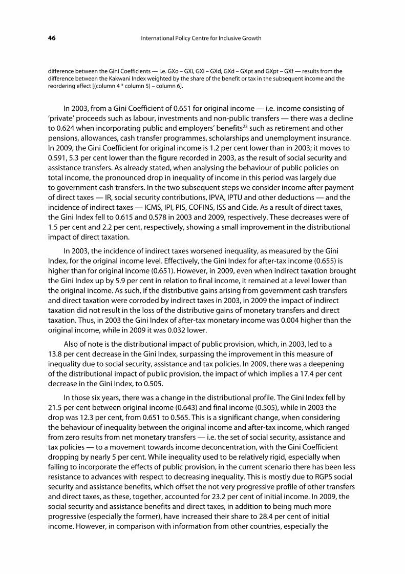
46 International Policy Centre for Inclusive Growth
difference between the Gini Coefficients — i.e. GXo – GXi, GXi – GXd, GXd – GXpt and GXpt – GXf — results from the difference between the Kakwani Index weighted by the share of the benefit or tax in the subsequent income and the reordering effect [(column 4 * column 5) – column 6].
In 2003, from a Gini Coefficient of 0.651 for original income — i.e. income consisting of ‘private’ proceeds such as labour, investments and non-public transfers — there was a decline to 0.624 when incorporating public and employers’ benefits23 such as retirement and other pensions, allowances, cash transfer programmes, scholarships and unemployment insurance. In 2009, the Gini Coefficient for original income is 1.2 per cent lower than in 2003; it moves to 0.591, 5.3 per cent lower than the figure recorded in 2003, as the result of social security and assistance transfers. As already stated, when analysing the behaviour of public policies on total income, the pronounced drop in inequality of income in this period was largely due to government cash transfers. In the two subsequent steps we consider income after payment of direct taxes — IR, social security contributions, IPVA, IPTU and other deductions — and the incidence of indirect taxes — ICMS, IPI, PIS, COFINS, ISS and Cide. As a result of direct taxes, the Gini Index fell to 0.615 and 0.578 in 2003 and 2009, respectively. These decreases were of 1.5 per cent and 2.2 per cent, respectively, showing a small improvement in the distributional impact of direct taxation.
In 2003, the incidence of indirect taxes worsened inequality, as measured by the Gini Index, for the original income level. Effectively, the Gini Index for after-tax income (0.655) is higher than for original income (0.651). However, in 2009, even when indirect taxation brought the Gini Index up by 5.9 per cent in relation to final income, it remained at a level lower than the original income. As such, if the distributive gains arising from government cash transfers and direct taxation were corroded by indirect taxes in 2003, in 2009 the impact of indirect taxation did not result in the loss of the distributive gains of monetary transfers and direct taxation. Thus, in 2003 the Gini Index of after-tax monetary income was 0.004 higher than the original income, while in 2009 it was 0.032 lower.
Also of note is the distributional impact of public provision, which, in 2003, led to a 13.8 per cent decrease in the Gini Index, surpassing the improvement in this measure of inequality due to social security, assistance and tax policies. In 2009, there was a deepening of the distributional impact of public provision, the impact of which implies a 17.4 per cent decrease in the Gini Index, to 0.505.
In those six years, there was a change in the distributional profile. The Gini Index fell by 21.5 per cent between original income (0.643) and final income (0.505), while in 2003 the drop was 12.3 per cent, from 0.651 to 0.565. This is a significant change, when considering the behaviour of inequality between the original income and after-tax income, which ranged from zero results from net monetary transfers — i.e. the set of social security, assistance and tax policies — to a movement towards income deconcentration, with the Gini Coefficient dropping by nearly 5 per cent. While inequality used to be relatively rigid, especially when failing to incorporate the effects of public provision, in the current scenario there has been less resistance to advances with respect to decreasing inequality. This is mostly due to RGPS social security and assistance benefits, which offset the not very progressive profile of other transfers and direct taxes, as these, together, accounted for 23.2 per cent of initial income. In 2009, the social security and assistance benefits and direct taxes, in addition to being much more progressive (especially the former), have increased their share to 28.4 per cent of initial income. However, in comparison with information from other countries, especially the

Working Paper 47
core Organisation for Economic Co-operation and Development (OECD) countries, we see that in those countries the share of benefits and direct taxes in income is more expressive, and policies on social security and the taxation of income and assets are more progressive.
In this period we also witnessed both a decrease in the share of indirect taxes in the initial income and an increase in the weight of public education, and, as stated, the total monetary income declared by households grew, in real terms, by almost 25 per cent between POFs.
Observation of the behaviour of the Kakwani Index between 2003 and 2009 indicates, roughly, an increase in the progressivity of monetary benefits and direct taxes and a decrease in the regressivity of indirect taxes. There was a significant increase in progressivity for all social security and assistance pensions, with the Kakwani Index going from 0.479 in 2003 to 0.734 in 2009. It is true that, among the benefits, the highest growth can be observed in retirement and other pensions in the public sector (RPPS), which is due, in some measure, to the fact that a portion of RPPS retirement pensions and other pensions of higher value has been declared as originating from RGPS. We must, however, emphasise that the PNAD data show that retirement and other pensions contributed to the reduction in inequality, because benefits greater than 4.5 minimum wages have lost ‘weight’ within income. On the other hand, the growth in the progressivity of aid and the sign change (from regressive to slightly progressive) for scholarships stand out. The Kakwani Progressivity Indices for PBF and BPC — not collected separately in the 2002–2003 POF — are quite high, demonstrating the distributive nature of these policies, which also boast marginal reordering effects.
In the case of direct taxes, there is tenuous growth in the Kakwani Index that measures the progressivity for all of them, with social security contributions showing a higher index, albeit not enough to change its neutral profile. The hypothesis is that the improvement in the progressivity of social security contributions reflects the impacts of the growth of formal employment in recent years, which incorporated average income segments into the labour market. Negative highlights are the almost complete neutrality of IPTU and IPVA in both POFs, which is not consistent with what is expected of asset taxation.
The regressivity of indirect taxes is illustrated by the Kakwani Index, which has remained around –0.13. In this case, the effects of IPI, which showed a significant change, from neutral to regressive, and the increased regressivity of ISS and Cide-fuels — explained by the increase in consumption of industrial goods, services and fuels by the poor and average income strata of the population — were offset by the decreased regressivity of ICMS. It is worth mentioning that, with the exception of IPI exemptions in 2009, changes in tax laws governing ICMS, ISS and Cide-fuels were marginal.
The breakdown of the Gini Index variance, the impact of the progressivity of the benefit or direct tax determined based on previous income, is mitigated by the reordering effect (column 6 of Tables 12 and 13). In the case of indirect taxes, characterised by being regressive, reordering reinforces income concentration — i.e. regressivity grows. The more significant effect of reordering is clear, in the case of benefits, when the progressivity index is calculated based on ex ante income.
In developed countries, the effects of reordering are also in direct opposition to the progressivity of benefits and direct taxes. They are, however, far less expressive. The changes between 2003 and 2009 did not cause any significant changes to this situation. In fact, given the magnitude of the progressivity component in direct taxes and benefits in developed countries, the concentrating effect of the reordering component is marginal, unlike in Brazil. As such, in the developed-country average analysed by de Beer et al. (2001), the reordering component represents 17 per cent of the progressivity component for benefits and 15 per cent

48 International Policy Centre for Inclusive Growth
for direct taxes; in Brazil, these figures reached 62 per cent and 15 per cent, respectively, in 2009. In 2003, the ratio between the concentrating effect of reordering and the distributive impact of benefits and direct taxes was 59 per cent and 27 per cent, respectively.
TABLE 14
Indicators of Progressivity (Lerman and Yitzhaki), Share in Income and the Effects of Reordering Benefits and Direct and Indirect Taxes, Brazil (2002–2003)
Benefits and taxes Gini
Differences
between
Gini Indices
(7)
Lerman and
Yitzhaki
Indices
(5)
Percentage
benefit or tax in
the previous
income
Reordering
(6)
Original income (Xo) 0.6509
Initial income (Benefits — b) (Xi) 0.6241 0.0268 0.0399 0.1583 0.0205
Disposable income (direct taxes — t) (Xd) 0.6148 0.0093 0.0663 0.0941 0.0030
Post‐tax income (Indirect taxes — ti) (Xpt) 0.6552 ‐0.0404 ‐0.2671 0.1948 0.0116
Final income (public education and health —
bnm) (Xf) 0.5649 0.0903 0.6663 0.1764 ‐0.0272
RGPS (1) 0.6574 0.0333 0.2404 0.0827 0.0134
RPPS (1) 0.6142 ‐0.0099 ‐0.2821 0.0543 0.0054
Aid (1) 0.6246 0.0005 0.3151 0.0013 0.0001
Scholarship (1) 0.6231 ‐0.0010 ‐0.3115 0.0040 0.0002
Cash transfer programmes (1) 0.6263 0.0022 0.8485 0.0025 0.0001
Unemployment insurance (1) 0.6245 0.0004 0.3197 0.0011 0.0000
Social security contributions (2) 0.6241 0.0000 ‐0.0149 0.0311 0.0004
Income tax (2) 0.6180 0.0061 0.2766 0.0209 0.0004
Property tax (IPTU) (2) 0.6247 ‐0.0006 ‐0.1051 0.0145 0.0009
Vehicle tax (IPVA) (2) 0.6237 0.0004 0.0665 0.0060 0.0000
Other discounts (2) 0.6211 0.0030 0.1031 0.0239 0.0005
ICMS (3) 0.6334 ‐0.0186 ‐0.2153 0.1030 0.0036
IPI (3) 0.6160 ‐0.0011 ‐0.0820 0.0346 0.0017
PIS‐Cofins (3) 0.6248 ‐0.0100 ‐0.1866 0.0593 0.0011
Cide fuels (3) 0.6148 0.0000 0.0027 0.0060 0.0000
ISS (3) 0.6149 0.0000 ‐0.0072 0.0060 0.0000
Public education (4) 0.6014 0.0539 0.7594 0.0963 ‐0.0193
Public health (4) 0.6115 0.0438 0.6242 0.0653 0.0030
Source: POF microdata (2002–2003)
Notes: (1): The Gini Indices refer to the initial income minus the benefit. The difference between the Gini Indices is the difference between the one relating to initial income and no benefit and the one relating to initial income. (2): The Gini Indices refer to the initial income minus direct taxation. The difference between the Gini Indices is the difference between the one relating to initial income and the one relating to initial income minus the tax. (3): The Gini Indices refer to disposable income minus the indirect tax. The difference between the Gini Indices is the difference between disposable income and disposable income minus indirect taxation. (4): The Gini Indices refer to the final income minus the benefit. The difference between the Gini indices lies between income net of taxes and final income minus the benefit. (5): GXi – Cb for benefits; Ct – Gd for direct taxes; Cti – Gpt for indirect taxes; and Cbnm – Gf for non-monetary benefits; with concentration ratios based on the ordering of households by subsequent income: initial, disposable, after taxes and final, respectively. GXo – CXo for benefits; GXi – CXi for direct taxes; GXd – CXd for indirect taxes; and GXf – CXf for indirect taxes; with concentration ratios based on the ordering of households by subsequent income: initial, disposable, after taxes and final, respectively. The differences between Gini Indices stem from the sum of the Lerman-Yitzhaki Index, weighted by the income share of the benefit or tax in the previous income and the effect of reordering [(column 4 * column 5) + column 6].

Working Paper 49
TABLE 15
Indicators of Progressivity (Lerman and Yitzhaki), Share in Income and the Effects of Reordering Benefits and Direct and Indirect Taxes, Brazil (2008–2009)
Benefits and taxes Gini
Differences
between Gini
Indices
(6)
Lerman
and
Yitzhaki
Indices
(4)
Ppercentage
benefit or tax in
the previous
income
Reordering
(5)
Original income (Xo) 0,6433
Initial income (Benefits — b) (Xi) 0,5909 0,0524 0,0592 0,2289 0,0389
Disposable income (direct taxes — t) (Xd) 0,5777 0,0132 0,1143 0,0981 0,0019
Income after taxation (indirect taxes — ti)
(Xpt) 0,6116 ‐0,0339 ‐0,2380 0,1713 0,0069
Final income (public education and health
— bnm) (Xf) 0,5054 0,1063 0,4709 0,2033 0,0105
RGPS (1) 0,6332 0,0424 0,1207 0,1320 0,0264
RPPS (1) 0,5861 ‐0,0048 ‐0,2334 0,0574 0,0086
Aid (1) 0,5924 0,0016 0,3758 0,0029 0,0005
Scholarship (1) 0,5908 0,0000 ‐0,1192 0,0015 0,0001
Cash transfer programmes (1) 0,5965 0,0057 1,0676 0,0052 0,0001
Unemployment insurance (1) 0,5917 0,0008 0,3160 0,0024 0,0001
BPC 0,5939 0,0031 0,6977 0,0034 0,0006
Social security contributions (2) 0,5891 0,0018 0,0483 0,0326 0,0002
Income tax (2) 0,5837 0,0071 0,3173 0,0220 0,0001
Property tax (IPTU) (2) 0,5909 ‐0,0001 ‐0,0368 0,0122 0,0004
Vehicle tax (IPVA) (2) 0,5904 0,0004 0,0487 0,0080 0,0000
Other discounts (2) 0,5878 0,0031 0,1101 0,0232 0,0005
ICMS (3) 0,5928 ‐0,0151 ‐0,1831 0,0903 0,0015
IPI (3) 0,5806 ‐0,0029 ‐0,1436 0,0208 0,0001
PIS‐Cofins (3) 0,5857 ‐0,0080 ‐0,1614 0,0521 0,0004
CIDE fuels (3) 0,5779 ‐0,0002 ‐0,0374 0,0051 0,0000
ISS (3) 0,5779 ‐0,0002 ‐0,0386 0,0030 ‐0,0001
Public education (4) 0,5479 0,0637 0,4714 0,1159 0,0090
Public health (4) 0,5586 0,0531 0,5972 0,0874 0,0009
Source: POF microdata (2008–2009)
Notes: (1): The Gini Indices refer to the initial income minus the benefit. The difference between the Gini Indices is the difference between the one relating to initial income and no benefit and the one relating to initial income. (2): The Gini Indices refer to the initial income minus direct taxation. The difference between the Gini Indices is the difference between the one relating to initial income and the one relating to initial income minus the tax. (3): The Gini Indices refer to disposable income minus the indirect tax. The difference between the Gini Indices is the difference between disposable income and disposable income minus indirect taxation. (4): The Gini Indices refer to the final income minus the benefit. The difference between the Gini indices lies between income net of taxes and final income minus the benefit. (5): GXi – Cb for benefits; Ct – Gd for direct taxes; Cti – Gpt for indirect taxes; and Cbnm – Gf for non-monetary benefits; with concentration ratios based on the ordering of households by subsequent income: initial, disposable, after taxes and final, respectively. GXo – CXo for benefits; GXi – CXi for direct taxes; GXd – CXd for indirect taxes; and GXf – CXf for indirect taxes; with concentration ratios based on the ordering of households by subsequent income: initial, disposable, after taxes and final, respectively. The differences between Gini Indices stem from the sum of the Lerman-Yitzhaki Index, weighted by the income share of the benefit or tax in the previous income and the effect of reordering [(column 4 * column 5) + column 6].

50 International Policy Centre for Inclusive Growth
Regarding the behaviour of public provision, there are opposing movements in the Kakwani Progressivity Indices for education and public health. The index for education has been growing, and the one for health has been declining, but both have been doing so weakly. On the other hand, both policies had increments in terms of income share, notably health. As a result, there were declines in the Gini Coefficient that were larger, both in absolute and in relative terms. The reordering effects were attenuated.
As shown in Tables 14 and 15, the Lerman-Yitzhaki Progressivity Indices of monetary and non-monetary benefits and of direct taxes are less progressive, and, in the case of direct taxation, the difference is less pronounced, especially in 2009. On the other hand, for indirect taxes, regressivity measured by the Lerman-Yitzhaki Index is more intense and is reduced by the ‘redistributive’ nature of reordering. The use of the two progressivity measures offers different perspectives for the analysis of changes in income inequality resulting from public policies.
Between 2003 and 2009, the Lerman-Yitzhaki Index captured the growth in the progressivity of cash benefits and direct taxation and the fall in the regressivity of indirect taxes. The progressivity of public education reduced, associated with a sign change in reordering effects, going from being a concentrator to a redistributor. Among social security and assistance benefits, it is worth noting the decreased regressivity of RPPS benefits and the decreased progressivity of those operated by RGPS. This decrease in the progressivity of RGPS retirement and other pensions is observed for both the Lerman-Yitzhaki Progressivity Index and the Kakwani Index, due to the appreciation of these benefits. Their share of original income increased from 8.3 per cent in 2003 to 12.1 per cent in 2009.
Public non-monetary benefits — education and health — boast the highest marginal distributive contributions, as a result of the combination of a significant share and a low concentration coefficient. Between 2003 and 2009 there was an increase in the importance of public education and health: their share of final income increased from 15.0 per cent to 16.9 per cent, associated with a slight decrease in the concentration ratio. We conclude that universal non-monetary benefits continue to have the greatest distributive impact of all public policies.
In the case of direct taxes, we note the increase in progressivity of the IR and the continued relatively neutral effect of social security contributions and IPVA. For indirect taxes, and similar to what was stated in the analysis of the Kakwani Index, we see an increase in IPI and sign changes in ISS and Cide-fuels.
5 FINAL CONSIDERATIONS
This paper sought to contribute to the debate on the tax burden, its size and the inequity of its application. This is, initially, because it sheds light on the profile of its counterpart, government spending — notably on social programmes — which, in recent years, has become much more progressive and has been responsible for a significant portion of the decline in inequality.
While we are focusing here on the distributive gains of social spending, this does not mean that less importance should be given to the distributional potential of changing the tax burden to increase the share of direct taxes, with a reduction of consumption taxes as a counterpart. Accordingly, we continue to follow the thinking of American jurist Oliver Wendell Holmes, synthesised in the sentence that illustrates the frontispiece of the Internal Revenue Service (IRS): “Taxes are what we pay for civilized society.” Recent experience has shown that

Working Paper 51
redistribution via spending is very effective and seems to encounter less resistance. We conclude that increases in asset taxation, through adjustments in the value of property, the institution of a progressive IPVA, the expansion of and increase in inheritance tax rates, the return of taxes on profits and dividends and changes to IRPF, to broaden its progressivity, would be much more resistant than increasing the minimum wage, introducing a large cash transfer programme such as PBF and increasing spending on health and education.
It is worth recalling that, in the past decade, most research efforts — Vianna et al. (2000), Magalhães et al. (2001), Silveira (2004), Silveira and Diniz (2005) and Silveira (2008) among others — have focused on assessing the tax incidence in Brazil and highlighting its regressivity. The objective was to propose changes in tax policy that would have distributional effects. We proposed changes to ICMS (Magalhães et al., 2000), to IRPF and to PIS-COFINS (Soares et al., 2009), and there were changes in the social security contributions of employees (Ansililero et al., 2010) and IPTU (Carvalho Jr., 2009). A major goal of this research was to point out ways to decrease Brazilian inequality, while taking tax issues into account. The exemption or extension of the exemption of essential products of the so-called food basket, changes to IRPF, with the reduction of tax benefits and the extension of ranges of incidence, and the exemption of the employee’s contribution to the first minimum wage were distributive proposals.
In short, the regressive profile of funding has not changed, and the progressivity of spending has greatly improved. Who can guarantee that changes in funding, on behalf of competitiveness, equity and efficiency, will not bring about changes in spending and in its current, more progressive nature? Our proposals are still available to be implemented, and, with them, we shall achieve greater equity in public interventions.

52 International Policy Centre for Inclusive Growth
REFERENCES
Afonso, J.R. (2010). ‘Fisco e equidade no Brasil’, Caderno de Pesquisa, No. 83. Campinas, Núcleo de Estudos de Políticas Publicas – UNICAMP.
Almeida, A.C. (2010). O dedo na ferida: menos imposto, mais consumo. Rio de Janeiro, Ed. Record.
Cardoso Jr., J.C. and J.A. Castro (2005). ‘Economia política das finanças sociais brasileiras no período 1995/2002’, X Encontro Nacional de Economia Política. Campinas, Instituto de Economia – UNICAMP.
Carvalho Jr., P.H.B. (2009). ‘Aspectos distributivos do IPTU e do patrimônio imobiliário das famílias’, Texto para Discussão, No. 1417. Rio de Janeiro, Ipea.
Castro, J.A. (2007). ‘Financiamento e gasto público na educação básica no Brasil: 1995–2005’, Educação e Sociedade, Vol. 28, No. 100: 857–876.
de Beer, P. et al. (2001). ‘Measuring welfare state performance: three or two worlds of welfare capitalism’, Luxembourg Income Study Working Paper, No. 276. The Hague, Social and Cultural Planning Office in the Netherlands, <http://www.lisdatacenter.org/wps/liswps/276.pdf> (accessed 16 July 2013).
Federação do Comércio do Estado de São Paulo (Fecomércio) (2006). Simplificando o Brasil: uma proposta da Fecomércio para o desenvolvimento sustentado. São Paulo, Editora Senac São Paulo.
Gobetti, S.W. and R.O. Orair (2010). ‘Classificação e análise das despesas públicas federais pela ótica macroeconómica (2002–2009)’, Texto para Discussão, No. 1485. Brasília, Ipea.
Hoffmann, R. (2007). ‘Medindo a regressividade das transferências’, in R.P. de Barros, M.N. Foguel and G. Ulyssea (eds), Desigualdade de renda no Brasil: uma análise da queda recente, Vol. 2. Brasília, Ipea.
Instituto de Pesquisa Econômica Aplicada (Ipea) (2011). ‘15 Anos de Gasto Social Federal Notas Sobre o Período de 1995 a 2009’, Comunicado do Ipea, No. 98. Brasília, Ipea.
Instituto de Pesquisa Econômica Aplicada (Ipea) (2010). ‘Efeitos econômicos do Gasto Social no Brasil’ in IPEA, Perspectivas da política social no Brasil – Série Eixos Estratégicos do Desenvolvimento Brasileiro: Proteção Social, Garantia de Direitos e Geração de Oportunidades, Vol. 8. Brasília: Ipea.
Instituto de Pesquisa Econômica Aplicada (Ipea) (2009). ‘Receita pública: Quem paga e como se gasta no Brasil’, Comunicado do Ipea, No. 22. Brasília, Ipea.
Jones, F. (2007). The effects of taxes and benefits on household income, 2005–06. London, Office for National Statistics, <http://www.ons.gov.uk/ons/rel/household-income/the-effects-of-taxes-and-benefits-on-household-income/2005-2006/index.html> (accessed 16 July 2013).
Lambert, P.J. (2001). The distribution and redistribution of income, 3rd edition. Manchester, Manchester University Press.
Lerman, R.I. and S. Yitzhaki (1995). ‘Changing ranks and the inequality impacts of taxes and transfers’, National Tax Journal, Vol. 48, No. 1, March.
Lerman, R.I. and S. Yitzhaki (1994). ‘Effect of marginal changes in income sources on U.S. income inequality’, Public Finance Quarterly, Vol. 22, October.

Working Paper 53
Magalhães, L.C.G., F.G. Silveira, F. A. Tomich and S.W. Vianna (2001). ‘Tributação sobre alimentação e seus impactos na distribuição de renda e pobreza nas grandes regiões urbanas brasileiras’, Economia, Vol. 2, No. 1, January/June.
Pintos-Payeras, J.A. (2010). ‘Análise da Progressividade da Carga Tributária sobre a População Brasileira’, Pesquisa e Planejamento Econômico, Vol. 40, No. 2, August.
Pintos-Payeras, J.A. (2008). ‘A carga tributária no Brasil e sua distribuição’, Doctoral thesis. São Paulo, ESALQ-UPS.
Ramos, C.A. (2001). ‘Aspectos distributivos do gasto público na saúde’, Planejamento e Políticas Públicas, No. 24, December.
Santos, C.H. (2010). ‘Um panorama das finanças públicas brasileiras de 1995 a 2009’, in J.A. Castro, C.H. Santos and J.A.C. Ribeiro (eds), Tributação e equidade no Brasil: um registro da reflexão do Ipea no biênio 2008–2009. Brasília, Ipea.
Silveira, F.G. (2010). ‘Tributação, Previdência e Assistência Sociais: impactos distributivos’, in J.A. Castro, C.H. Santos and J.A.C. Ribeiro (eds), Tributação e equidade no Brasil: um registro da reflexão do Ipea no biênio 2008–2009. Brasília, Ipea.
Silveira, F.G. (2008). ‘Tributação, Previdência e Assistência Sociais: Impactos Distributivos’, Doctoral thesis. Campinas, UNICAMP.
Silveira, F.G. (2003). ‘Impacto das transferências governamentais e da tributação na distribuição de renda no Brasil’, Econômica, Vol. 5, No. 1, June: 171–184.
Silveira, F.G. and B.C. Diniz (2005). ‘A incidência da tributação direta no País: o que dizem os dados da Pesquisa de Orçamentos Familiares de 2002/03’, Informações Fipe, No. 297. São Paulo, Fundação Instituto de Pesquisas Econômicas.
Soares, S., F.G. Silveira, F.M. Santos and A.L. Souza (2010). ‘O potencial distributivo do Imposto de Renda Pessoa Física (IRPF)’, in J.A. Castro, C.H. Santos and J.A.C. Ribeiro (eds), Tributação e equidade no Brasil: um registro da reflexão do Ipea no biênio 2008–2009. Brasília, Ipea.
Vianna, S.T.W. (2000). ‘Tributação sobre renda e consumo das famílias no Brasil: avaliação de sua incidência nas grandes regiões urbanas em 1996’, Dissertation, Master’s in Economics. Rio de Janeiro, Institute of Economics, Federal University of Rio de Janeiro.
Vianna, S.T.W., L.C.G. Magalhães, F.G. Silveira and F.A. Tomich (2000). ‘Carga Tributária Direta e Indireta sobre as Unidades Familiares no Brasil: Avaliação de sua Incidência nas Grandes Regiões Urbanas em 1996’, Texto para Discussão, No. 757. Brasília, Ipea.
Zockun, M.H. (2005). ‘Aumenta a regressividade dos impostos no Brasil’, Informações Fipe, No. 297. São Paulo, Fundação Instituto de Pesquisas Econômicas.


NOTES
1. Final income refers to all income received privately, plus public monetary and non-monetary transfers and minus direct and indirect taxes. Additional details of income stages and public policy — social security and assistance, tax and public provision of health and education — are presented subsequently and illustrated in Figure 1.
2. See: <http://www.receita.fazenda.gov.br/principal/Ingles/SistemaTributarioBR/Taxes.htm>.
3. Specifically, the question posed is: ‘With which statement do you most agree: i) it is better for the population if the government reduces taxes and has fewer civil servants, which would reduce product prices, ii) it is better for the poor population if there are more taxes and that the tax money be used by the government in more social programmes.’
4. For an analysis of the behaviour of the tax burden in recent years, see Santos (2010).
5. Unfortunately, we are not very clear on all that is encompassed by ‘other deductions’ because, according to research manuals (especially for interviewers) this would include, primarily, the ISS, and exclude FGTS collection. Note that, when analysing workers who claim ‘other deductions’, we find people (civil servants, military and private-sector employees) on whom this tax is not levied.
6. Here we consider the ISS paid by freelancers and the self-employed. The person analysed may have, to some extent, declared the taxes paid by companies when paying a freelancer — the individual in question.
7. It is worth noting that sanitation expenditures are also accounted for, covered together with health.
8. In fact, the RGPS database has a much greater wealth of information available than the RPPS database. For federal government retirees and pensioners, there is information available from the MPS’s Statistical Staff Bulletin, which shows the number of beneficiaries and the amount paid, in amount ranges. In 2003, these ranges were defined by multiples of the minimum wage and, thus, were rendered compatible with the data available in the social security database.
9. Available at:<http://www1.previdencia.gov.br/sps/app/dempre/default.asp>.
10. Since this amount was higher than the amount captured by the 2002–2003 POF, an adjustment factor was applied to the retirement and other pension amounts found in the administrative records of the two regimes (RGPS and RPPSs), so as to adapt them to the POF.
11. This topic is based on the works of Lambert (2001), Hoffman (2007) and Yitzhaki and Lerman (1994; 1995).
12. The following presentation is based on Hoffmann (2007).
13. For more details, see Lambert (2001).
14. Hoffmann (2007) supports the use of the term ‘progressivity’ for the benefits that contribute to the fall in inequality, unlike Lambert (2001). He argues that “the terms ‘progressive’ and ‘regressive’ are directly linked to the idea of smaller and greater inequality”.
15. The Kakwani Index weighted by the share of the element under analysis (tax or benefit) was later named by Lambert (2001: 207) as the Reynolds and Smolensky Index.
16. “In particular, estimates of global effects of a tax or transfer will depend on the order in which the source is entered. For example, the inequality impact of the social security tax will differ depending on whether one deducts social security taxes from gross income or from income net of personal income taxes. A major reason is that the rankings differ with each income concept” (Lerman and Yitzhaki, 1995: 45–46).
17. D stands for direct taxes, and t stands for the total taxes — direct and indirect.
18. Ct is the concentration ratio of taxes, with families ordered by subsequent incomes.
19. “We favour the use of equation 4 [similar to 14], partly because we think that the after-tax ranking is the appropriate ranking for calculating progressivity” (Lerman and Yitzhaki, 1995: 51).
20. We note that this is about the tax collected by freelance professionals and self-employed service providers.
21. Here we consider the ISS embedded in the prices of goods and services — i.e. ISS as an indirect tax.
22. In using the total income determined by the POF, there is some level of double counting, because part of public spending on health and education is captured by the POF, through non-monetary income (expenses). Indeed, the non-monetary income investigated by the POF includes the rent estimated for families who reside in their own properties — or rent properties — production for one’s own consumption, withdrawal of business, donations and other non-cash expenses, covering goods only. Thus, the POF investigates educational and health goods, such as school meals and supplies, medicine and medical examinations. We argue, however, that the double counting is not at all significant, since a large part of public spending on education and, to a lesser extent, health, goes to services, not goods. Moreover, the inclusion of these goods as non-monetary expenses is quite minimal.
23. In this case, these are benefits granted by public and private employers as a result of labour agreements.

International
Centre for Inclusive Growth
International Policy Centre for Inclusive Growth (IPC - IG)United Nations Development Programme
SBS, Quadra 1, Bloco J, Ed. BNDES, 13º andar
70076-900 Brasilia, DF - BrazilTelephone: +55 61 2105 5000
E-mail: [email protected] URL: www.ipc-undp.org