first-order logic - university of...

Part I

First-order Logic

1

Chapter 1

Syntax and Semantics

1.1 Introduction

fol:syn:int:sec

In order to develop the theory and metatheory of first-order logic, we mustfirst define the syntax and semantics of its expressions. The expressions of first-order logic are terms and formulas. Terms are formed from variables, constantsymbols, and function symbols. Formulas, in turn, are formed from predicatesymbols together with terms (these form the smallest, “atomic” formulas), andthen from atomic formulas we can form more complex ones using logical connec-tives and quantifiers. There are many different ways to set down the formationrules; we give just one possible one. Other systems will chose different symbols,will select different sets of connectives as primitive, will use parentheses differ-ently (or even not at all, as in the case of so-called Polish notation). What allapproaches have in common, though, is that the formation rules define the setof terms and formulas inductively. If done properly, every expression can re-sult essentially in only one way according to the formation rules. The inductivedefinition resulting in expressions that are uniquely readable means we can givemeanings to these expressions using the same method—inductive definition.

Giving the meaning of expressions is the domain of semantics. The centralconcept in semantics is that of satisfaction in a structure. A structure givesmeaning to the building blocks of the language: a domain is a non-emptyset of objects. The quantifiers are interpreted as ranging over this domain,constant symbols are assigned elements in the domain, function symbols areassigned functions from the domain to itself, and predicate symbols are assignedrelations on the domain. The domain together with assignments to the basicvocabulary constitutes a structure. Variables may appear in formulas, and inorder to give a semantics, we also have to assign elements of the domain tothem—this is a variable assignment. The satisfaction relation, finally, bringsthese together. A formula may be satisfied in a structure M relative to avariable assignment s, written as M, s |= ϕ. This relation is also defined byinduction on the structure of ϕ, using the truth tables for the logical connectivesto define, say, satisfaction of ϕ ∧ ψ in terms of satisfaction (or not) of ϕ and

3

ψ. It then turns out that the variable assignment is irrelevant if the formula ϕis a sentence, i.e., has no free variables, and so we can talk of sentences beingsimply satisfied (or not) in structures.

On the basis of the satisfaction relation M |= ϕ for sentences we can thendefine the basic semantic notions of validity, entailment, and satisfiability. Asentence is valid, ϕ, if every structure satisfies it. It is entailed by a set ofsentences, Γ ϕ, if every structure that satisfies all the sentences in Γ alsosatisfies ϕ. And a set of sentences is satisfiable if some structure satisfies allsentences in it at the same time. Because formulas are inductively defined, andsatisfaction is in turn defined by induction on the structure of formulas, we canuse induction to prove properties of our semantics and to relate the semanticnotions defined.

1.2 First-Order Languages

fol:syn:fol:sec

Expressions of first-order logic are built up from a basic vocabulary con-taining variables, constant symbols, predicate symbols and sometimes functionsymbols. From them, together with logical connectives, quantifiers, and punc-tuation symbols such as parentheses and commas, terms and formulas areformed.

explanation Informally, predicate symbols are names for properties and relations, con-stant symbols are names for individual objects, and function symbols are namesfor mappings. These, except for the identity predicate =, are the non-logicalsymbols and together make up a language. Any first-order language L is deter-mined by its non-logical symbols. In the most general case, L contains infinitelymany symbols of each kind.

In the general case, we make use of the following symbols in first-order logic:

1. Logical symbols

a) Logical connectives: ¬ (negation), ∧ (conjunction), ∨ (disjunction),→ (conditional), ↔ (biconditional), ∀ (universal quantifier), ∃ (ex-istential quantifier).

b) The propositional constant for falsity ⊥.

c) The propositional constant for truth >.

d) The two-place identity predicate =.

e) A denumerable set of variables: v0, v1, v2, . . .

2. Non-logical symbols, making up the standard language of first-order logic

a) A denumerable set of n-place predicate symbols for each n > 0: An0 ,An1 , An2 , . . .

b) A denumerable set of constant symbols: c0, c1, c2, . . . .

c) A denumerable set of n-place function symbols for each n > 0: f n0 ,f n1 , f n2 , . . .

4 first-order-logic by OLP / CC–BY

https://github.com/OpenLogicProject/OpenLogic

http://openlogicproject.org/

http://creativecommons.org/licenses/by/4.0/

3. Punctuation marks: (, ), and the comma.

Most of our definitions and results will be formulated for the full standardlanguage of first-order logic. However, depending on the application, we mayalso restrict the language to only a few predicate symbols, constant symbols,and function symbols.

Example 1.1. The language LA of arithmetic contains a single two-place pred-icate symbol <, a single constant symbol , one one-place function symbol ′,and two two-place function symbols + and ×.

Example 1.2. The language of set theory LZ contains only the single two-place predicate symbol ∈.

Example 1.3. The language of orders L≤ contains only the two-place predi-cate symbol ≤.

Again, these are conventions: officially, these are just aliases, e.g., <, ∈,and ≤ are aliases for A20, for c0, ′ for f 10 , + for f 20 , × for f 21 .

introYou may be familiar with different terminology and symbols than the oneswe use above. Logic texts (and teachers) commonly use either ∼, ¬, and ! for“negation”, ∧, ·, and & for “conjunction”. Commonly used symbols for the“conditional” or “implication” are→, ⇒, and ⊃. Symbols for “biconditional,”“bi-implication,” or “(material) equivalence” are ↔, ⇔, and ≡. The ⊥ sym-bol is variously called “falsity,” “falsum,”, “absurdity,”, or “bottom.” The >symbol is variously called “truth,” “verum,”, or “top.”

It is conventional to use lower case letters (e.g., a, b, c) from the beginningof the Latin alphabet for constant symbols (sometimes called names), and lowercase letters from the end (e.g., x, y, z) for variables. Quantifiers combine withvariables, e.g., x; notational variations include ∀x, (∀x), (x), Πx,

∧x for the

universal quantifier and ∃x, (∃x), (Ex), Σx,∨x for the existential quantifier.

explanationWe might treat all the propositional operators and both quantifiers as prim-itive symbols of the language. We might instead choose a smaller stock ofprimitive symbols and treat the other logical operators as defined. “Truthfunctionally complete” sets of Boolean operators include ¬,∨, ¬,∧, and¬,→—these can be combined with either quantifier for an expressively com-plete first-order language.

You may be familiar with two other logical operators: the Sheffer stroke |(named after Henry Sheffer), and Peirce’s arrow ↓, also known as Quine’s dag-ger. When given their usual readings of “nand” and “nor” (respectively), theseoperators are truth functionally complete by themselves.

1.3 Terms and Formulas

fol:syn:frm:sec

Once a first-order language L is given, we can define expressions built upfrom the basic vocabulary of L. These include in particular terms and formulas.

first-order-logic by OLP / CC–BY 5




Definition 1.4 (Terms). fol:syn:frm:

defn:terms

The set of terms Trm(L) of L is defined inductivelyby:

1. Every variable is a term.

2. Every constant symbol of L is a term.

3. If f is an n-place function symbol and t1, . . . , tn are terms, then f(t1, . . . , tn)is a term.

4. Nothing else is a term.

A term containing no variables is a closed term.

explanation The constant symbols appear in our specification of the language and theterms as a separate category of symbols, but they could instead have beenincluded as zero-place function symbols. We could then do without the secondclause in the definition of terms. We just have to understand f(t1, . . . , tn) asjust f by itself if n = 0.

Definition 1.5 (Formula). fol:syn:frm:

defn:formulas

The set of formulas Frm(L) of the language L isdefined inductively as follows:

1. ⊥ is an atomic formula.

2. > is an atomic formula.

3. If R is an n-place predicate symbol of L and t1, . . . , tn are terms of L,then R(t1, . . . , tn) is an atomic formula.

4. If t1 and t2 are terms of L, then =(t1, t2) is an atomic formula.

5. If ϕ is a formula, then ¬ϕ is formula.

6. If ϕ and ψ are formulas, then (ϕ ∧ ψ) is a formula.

7. If ϕ and ψ are formulas, then (ϕ ∨ ψ) is a formula.

8. If ϕ and ψ are formulas, then (ϕ→ ψ) is a formula.

9. If ϕ and ψ are formulas, then (ϕ↔ ψ) is a formula.

10. If ϕ is a formula and x is a variable, then ∀xϕ is a formula.

11. If ϕ is a formula and x is a variable, then ∃xϕ is a formula.

12. Nothing else is a formula.





explanationThe definitions of the set of terms and that of formulas are inductive defi-nitions. Essentially, we construct the set of formulas in infinitely many stages.In the initial stage, we pronounce all atomic formulas to be formulas; thiscorresponds to the first few cases of the definition, i.e., the cases for >, ⊥,R(t1, . . . , tn) and =(t1, t2). “Atomic formula” thus means any formula of thisform.

The other cases of the definition give rules for constructing new formulasout of formulas already constructed. At the second stage, we can use them toconstruct formulas out of atomic formulas. At the third stage, we constructnew formulas from the atomic formulas and those obtained in the second stage,and so on. A formula is anything that is eventually constructed at such a stage,and nothing else.

By convention, we write = between its arguments and leave out the paren-theses: t1 = t2 is an abbreviation for =(t1, t2). Moreover, ¬=(t1, t2) is ab-breviated as t1 6= t2. When writing a formula (ψ ∗ χ) constructed from ψ, χusing a two-place connective ∗, we will often leave out the outermost pair ofparentheses and write simply ψ ∗ χ.

introSome logic texts require that the variable x must occur in ϕ in order for∃xϕ and ∀xϕ to count as formulas. Nothing bad happens if you don’t requirethis, and it makes things easier.

If we work in a language for a specific application, we will often write two-place predicate symbols and function symbols between the respective terms,e.g., t1 < t2 and (t1 + t2) in the language of arithmetic and t1 ∈ t2 in thelanguage of set theory. The successor function in the language of arithmeticis even written conventionally after its argument: t′. Officially, however, theseare just conventional abbreviations for A20(t1, t2), f 20 (t1, t2), A20(t1, t2) and f10 (t),respectively.

Definition 1.6 (Syntactic identity). The symbol≡ expresses syntactic identitybetween strings of symbols, i.e., ϕ ≡ ψ iff ϕ and ψ are strings of symbols ofthe same length and which contain the same symbol in each place.

The ≡ symbol may be flanked by strings obtained by concatenation, e.g.,ϕ ≡ (ψ ∨ χ) means: the string of symbols ϕ is the same string as the oneobtained by concatenating an opening parenthesis, the string ψ, the ∨ symbol,the string χ, and a closing parenthesis, in this order. If this is the case, thenwe know that the first symbol of ϕ is an opening parenthesis, ϕ contains ψ as asubstring (starting at the second symbol), that substring is followed by ∨, etc.

1.4 Unique Readability

fol:syn:unq:sec

explanationThe way we defined formulas guarantees that every formula has a uniquereading, i.e., there is essentially only one way of constructing it according toour formation rules for formulas and only one way of “interpreting” it. If thiswere not so, we would have ambiguous formulas, i.e., formulas that have morethan one reading or intepretation—and that is clearly something we want to





avoid. But more importantly, without this property, most of the definitionsand proofs we are going to give will not go through.

Perhaps the best way to make this clear is to see what would happen if wehad given bad rules for forming formulas that would not guarantee unique read-ability. For instance, we could have forgotten the parentheses in the formationrules for connectives, e.g., we might have allowed this:

If ϕ and ψ are formulas, then so is ϕ→ ψ.

Starting from an atomic formula θ, this would allow us to form θ → θ. Fromthis, together with θ, we would get θ → θ → θ. But there are two ways to dothis:

1. We take θ to be ϕ and θ → θ to be ψ.

2. We take ϕ to be θ → θ and ψ is θ.

Correspondingly, there are two ways to “read” the formula θ → θ → θ. It is ofthe form ψ → χ where ψ is θ and χ is θ → θ, but it is also of the form ψ → χwith ψ being θ → θ and χ being θ.

If this happens, our definitions will not always work. For instance, when wedefine the main operator of a formula, we say: in a formula of the form ψ → χ,the main operator is the indicated occurrence of →. But if we can match theformula θ → θ → θ with ψ → χ in the two different ways mentioned above,then in one case we get the first occurrence of → as the main operator, andin the second case the second occurrence. But we intend the main operator tobe a function of the formula, i.e., every formula must have exactly one mainoperator occurrence.

Lemma 1.7. The number of left and right parentheses in a formula ϕ areequal.

Proof. We prove this by induction on the way ϕ is constructed. This requirestwo things: (a) We have to prove first that all atomic formulas have the prop-erty in question (the induction basis). (b) Then we have to prove that whenwe construct new formulas out of given formulas, the new formulas have theproperty provided the old ones do.

Let l(ϕ) be the number of left parentheses, and r(ϕ) the number of rightparentheses in ϕ, and l(t) and r(t) similarly the number of left and right paren-theses in a term t. We leave the proof that for any term t, l(t) = r(t) as anexercise.

1. ϕ ≡ ⊥: ϕ has 0 left and 0 right parentheses.

2. ϕ ≡ >: ϕ has 0 left and 0 right parentheses.

3. ϕ ≡ R(t1, . . . , tn): l(ϕ) = 1+ l(t1)+ · · ·+ l(tn) = 1+r(t1)+ · · ·+r(tn) =r(ϕ). Here we make use of the fact, left as an exercise, that l(t) = r(t)for any term t.





4. ϕ ≡ t1 = t2: l(ϕ) = l(t1) + l(t2) = r(t1) + r(t2) = r(ϕ).

5. ϕ ≡ ¬ψ: By induction hypothesis, l(ψ) = r(ψ). Thus l(ϕ) = l(ψ) =r(ψ) = r(ϕ).

6. ϕ ≡ (ψ ∗ χ): By induction hypothesis, l(ψ) = r(ψ) and l(χ) = r(χ).Thus l(ϕ) = 1 + l(ψ) + l(χ) = 1 + r(ψ) + r(χ) = r(ϕ).

7. ϕ ≡ ∀xψ: By induction hypothesis, l(ψ) = r(ψ). Thus, l(ϕ) = l(ψ) =r(ψ) = r(ϕ).

8. ϕ ≡ ∃xψ: Similarly.

Definition 1.8 (Proper prefix). A string of symbols ψ is a proper prefix ofa string of symbols ϕ if concatenating ψ and a non-empty string of symbolsyields ϕ.

Lemma 1.9.fol:syn:unq:

lem:no-prefix

If ϕ is a formula, and ψ is a proper prefix of ϕ, then ψ is nota formula.

Proof. Exercise.

Problem 1.1. Prove Lemma 1.9.

Proposition 1.10.fol:syn:unq:

prop:unique-atomic

If ϕ is an atomic formula, then it satisfes one, and onlyone of the following conditions.

1. ϕ ≡ ⊥.

2. ϕ ≡ >.

3. ϕ ≡ R(t1, . . . , tn) where R is an n-place predicate symbol, t1, . . . , tn areterms, and each of R, t1, . . . , tn is uniquely determined.

4. ϕ ≡ t1 = t2 where t1 and t2 are uniquely determined terms.

Proof. Exercise.

Problem 1.2. Prove Proposition 1.10 (Hint: Formulate and prove a versionof Lemma 1.9 for terms.)

Proposition 1.11 (Unique Readability). Every formula satisfies one, and onlyone of the following conditions.

1. ϕ is atomic.

2. ϕ is of the form ¬ψ.

3. ϕ is of the form (ψ ∧ χ).

4. ϕ is of the form (ψ ∨ χ).





5. ϕ is of the form (ψ → χ).

6. ϕ is of the form (ψ ↔ χ).

7. ϕ is of the form ∀xψ.

8. ϕ is of the form ∃xψ.

Moreover, in each case ψ, or ψ and χ, are uniquely determined. This meansthat, e.g., there are no different pairs ψ, χ and ψ′, χ′ so that ϕ is both of theform (ψ → χ) and (ψ′ → χ′).

Proof. The formation rules require that if a formula is not atomic, it must startwith an opening parenthesis (, ¬, or with a quantifier. On the other hand,every formula that start with one of the following symbols must be atomic:a predicate symbol, a function symbol, a constant symbol, ⊥, >.

So we really only have to show that if ϕ is of the form (ψ ∗ χ) and also ofthe form (ψ′ ∗′ χ′), then ψ ≡ ψ′, χ ≡ χ′, and ∗ = ∗′.

So suppose both ϕ ≡ (ψ ∗χ) and ϕ ≡ (ψ′ ∗′ χ′). Then either ψ ≡ ψ′ or not.If it is, clearly ∗ = ∗′ and χ ≡ χ′, since they then are substrings of ϕ that beginin the same place and are of the same length. The other case is ψ 6≡ ψ′. Sinceψ and ψ′ are both substrings of ϕ that begin at the same place, one must bea proper prefix of the other. But this is impossible by Lemma 1.9.

1.5 Main operator of a Formula

fol:syn:mai:sec

explanation It is often useful to talk about the last operator used in constructing aformula ϕ. This operator is called the main operator of ϕ. Intuitively, it is the“outermost” operator of ϕ. For example, the main operator of ¬ϕ is ¬, themain operator of (ϕ ∨ ψ) is ∨, etc.

Definition 1.12 (Main operator). fol:syn:mai:

def:main-op

The main operator of a formula ϕ is definedas follows:

1. ϕ is atomic: ϕ has no main operator.

2. ϕ ≡ ¬ψ: the main operator of ϕ is ¬.

3. ϕ ≡ (ψ ∧ χ): the main operator of ϕ is ∧.

4. ϕ ≡ (ψ ∨ χ): the main operator of ϕ is ∨.

5. ϕ ≡ (ψ → χ): the main operator of ϕ is →.

6. ϕ ≡ (ψ ↔ χ): the main operator of ϕ is ↔.

7. ϕ ≡ ∀xψ: the main operator of ϕ is ∀.

8. ϕ ≡ ∃xψ: the main operator of ϕ is ∃.





In each case, we intend the specific indicated occurrence of the main oper-ator in the formula. For instance, since the formula ((θ → α)→ (α→ θ)) is ofthe form (ψ → χ) where ψ is (θ → α) and χ is (α→ θ), the second occurrenceof → is the main operator.

explanationThis is a recursive definition of a function which maps all non-atomic formu-las to their main operator occurrence. Because of the way formulas are definedinductively, every formula ϕ satisfies one of the cases in Definition 1.12. Thisguarantees that for each non-atomic formula ϕ a main operator exists. Becauseeach formula satisfies only one of these conditions, and because the smaller for-mulas from which ϕ is constructed are uniquely determined in each case, themain operator occurrence of ϕ is unique, and so we have defined a function.

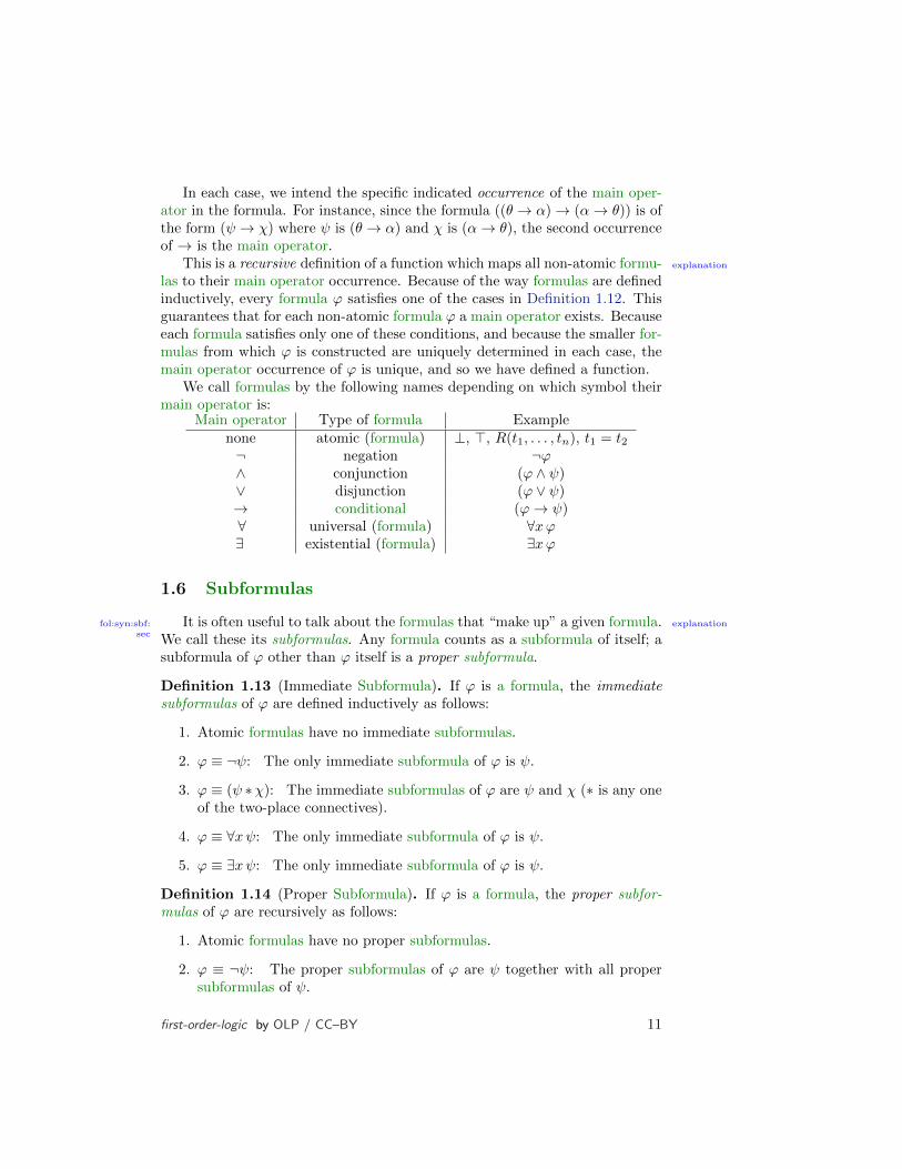
We call formulas by the following names depending on which symbol theirmain operator is:

Main operator Type of formula Examplenone atomic (formula) ⊥, >, R(t1, . . . , tn), t1 = t2¬ negation ¬ϕ∧ conjunction (ϕ ∧ ψ)∨ disjunction (ϕ ∨ ψ)→ conditional (ϕ→ ψ)∀ universal (formula) ∀xϕ∃ existential (formula) ∃xϕ

1.6 Subformulas

fol:syn:sbf:sec

explanationIt is often useful to talk about the formulas that “make up” a given formula.We call these its subformulas. Any formula counts as a subformula of itself; asubformula of ϕ other than ϕ itself is a proper subformula.

Definition 1.13 (Immediate Subformula). If ϕ is a formula, the immediatesubformulas of ϕ are defined inductively as follows:

1. Atomic formulas have no immediate subformulas.

2. ϕ ≡ ¬ψ: The only immediate subformula of ϕ is ψ.

3. ϕ ≡ (ψ ∗χ): The immediate subformulas of ϕ are ψ and χ (∗ is any oneof the two-place connectives).

4. ϕ ≡ ∀xψ: The only immediate subformula of ϕ is ψ.

5. ϕ ≡ ∃xψ: The only immediate subformula of ϕ is ψ.

Definition 1.14 (Proper Subformula). If ϕ is a formula, the proper subfor-mulas of ϕ are recursively as follows:

1. Atomic formulas have no proper subformulas.

2. ϕ ≡ ¬ψ: The proper subformulas of ϕ are ψ together with all propersubformulas of ψ.





3. ϕ ≡ (ψ ∗ χ): The proper subformulas of ϕ are ψ, χ, together with allproper subformulas of ψ and those of χ.

4. ϕ ≡ ∀xψ: The proper subformulas of ϕ are ψ together with all propersubformulas of ψ.

5. ϕ ≡ ∃xψ: The proper subformulas of ϕ are ψ together with all propersubformulas of ψ.

Definition 1.15 (Subformula). The subformulas of ϕ are ϕ itself togetherwith all its proper subformulas.

explanation Note the subtle difference in how we have defined immediate subformulasand proper subformulas. In the first case, we have directly defined the imme-diate subformulas of a formula ϕ for each possible form of ϕ. It is an explicitdefinition by cases, and the cases mirror the inductive definition of the set offormulas. In the second case, we have also mirrored the way the set of allformulas is defined, but in each case we have also included the proper subfor-mulas of the smaller formulas ψ, χ in addition to these formulas themselves.This makes the definition recursive. In general, a definition of a function onan inductively defined set (in our case, formulas) is recursive if the cases in thedefinition of the function make use of the function itself. To be well defined,we must make sure, however, that we only ever use the values of the functionfor arguments that come “before” the one we are defining—in our case, whendefining “proper subformula” for (ψ ∗ χ) we only use the proper subformulasof the “earlier” formulas ψ and χ.

1.7 Free Variables and Sentences

fol:syn:fvs:sec

Definition 1.16 (Free occurrences of a variable). fol:syn:fvs:

defn:free-occ

The free occurrences of avariable in a formula are defined inductively as follows:

1. ϕ is atomic: all variable occurrences in ϕ are free.

2. ϕ ≡ ¬ψ: the free variable occurrences of ϕ are exactly those of ψ.

3. ϕ ≡ (ψ ∗ χ): the free variable occurrences of ϕ are those in ψ togetherwith those in χ.

4. ϕ ≡ ∀xψ: the free variable occurrences in ϕ are all of those in ψ exceptfor occurrences of x.

5. ϕ ≡ ∃xψ: the free variable occurrences in ϕ are all of those in ψ exceptfor occurrences of x.

Definition 1.17 (Bound Variables). An occurrence of a variable in a formula ϕis bound if it is not free.





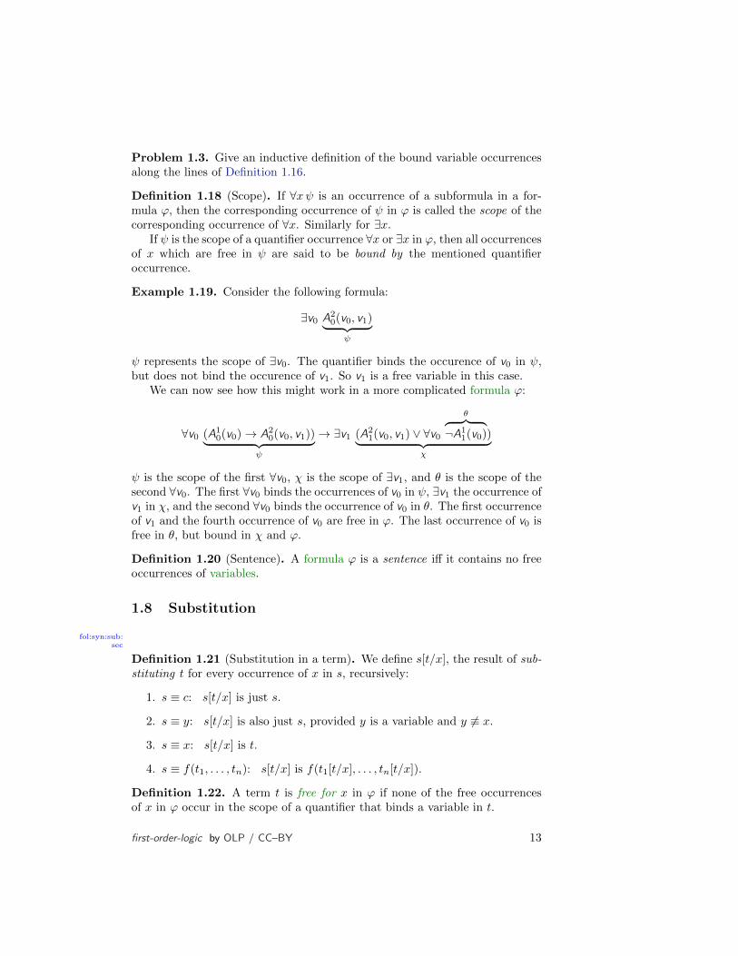
Problem 1.3. Give an inductive definition of the bound variable occurrencesalong the lines of Definition 1.16.

Definition 1.18 (Scope). If ∀xψ is an occurrence of a subformula in a for-mula ϕ, then the corresponding occurrence of ψ in ϕ is called the scope of thecorresponding occurrence of ∀x. Similarly for ∃x.

If ψ is the scope of a quantifier occurrence ∀x or ∃x in ϕ, then all occurrencesof x which are free in ψ are said to be bound by the mentioned quantifieroccurrence.

Example 1.19. Consider the following formula:

∃v0 A20(v0, v1)︸︷︷︸ψ

ψ represents the scope of ∃v0. The quantifier binds the occurence of v0 in ψ,but does not bind the occurence of v1. So v1 is a free variable in this case.

We can now see how this might work in a more complicated formula ϕ:

∀v0 (A10(v0)→ A20(v0, v1))︸︷︷︸ψ

→ ∃v1 (A21(v0, v1) ∨ ∀v0

θ︷︸︸︷¬A11(v0))︸︷︷︸

χ

ψ is the scope of the first ∀v0, χ is the scope of ∃v1, and θ is the scope of thesecond ∀v0. The first ∀v0 binds the occurrences of v0 in ψ, ∃v1 the occurrence ofv1 in χ, and the second ∀v0 binds the occurrence of v0 in θ. The first occurrenceof v1 and the fourth occurrence of v0 are free in ϕ. The last occurrence of v0 isfree in θ, but bound in χ and ϕ.

Definition 1.20 (Sentence). A formula ϕ is a sentence iff it contains no freeoccurrences of variables.

1.8 Substitution

fol:syn:sub:sec

Definition 1.21 (Substitution in a term). We define s[t/x], the result of sub-stituting t for every occurrence of x in s, recursively:

1. s ≡ c: s[t/x] is just s.

2. s ≡ y: s[t/x] is also just s, provided y is a variable and y 6≡ x.

3. s ≡ x: s[t/x] is t.

4. s ≡ f(t1, . . . , tn): s[t/x] is f(t1[t/x], . . . , tn[t/x]).

Definition 1.22. A term t is free for x in ϕ if none of the free occurrencesof x in ϕ occur in the scope of a quantifier that binds a variable in t.





Example 1.23.

1. v8 is free for v1 in ∃v3A24(v3, v1)

2. f 21 (v1, v2) is not free for vo in ∀v2A24(v0, v2)

Definition 1.24 (Substitution in a formula). If ϕ is a formula, x is a variable,and t is a term free for x in ϕ, then ϕ[t/x] is the result of substituting t for allfree occurrences of x in ϕ.

1. ϕ ≡ ⊥: ϕ[t/x] is ⊥.

2. ϕ ≡ >: ϕ[t/x] is >.

3. ϕ ≡ P (t1, . . . , tn): ϕ[t/x] is P (t1[t/x], . . . , tn[t/x]).

4. ϕ ≡ t1 = t2: ϕ[t/x] is t1[t/x] = t2[t/x].

5. ϕ ≡ ¬ψ: ϕ[t/x] is ¬ψ[t/x].

6. ϕ ≡ (ψ ∧ χ): ϕ[t/x] is (ψ[t/x] ∧ χ[t/x]).

7. ϕ ≡ (ψ ∨ χ): ϕ[t/x] is (ψ[t/x] ∨ χ[t/x]).

8. ϕ ≡ (ψ → χ): ϕ[t/x] is (ψ[t/x]→ χ[t/x]).

9. ϕ ≡ (ψ ↔ χ): ϕ[t/x] is (ψ[t/x]↔ χ[t/x]).

10. ϕ ≡ ∀y ψ: ϕ[t/x] is ∀y ψ[t/x], provided y is a variable other than x;otherwise ϕ[t/x] is just ϕ.

11. ϕ ≡ ∃y ψ: ϕ[t/x] is ∃y ψ[t/x], provided y is a variable other than x;otherwise ϕ[t/x] is just ϕ.

explanation Note that substitution may be vacuous: If x does not occur in ϕ at all, thenϕ[t/x] is just ϕ.

The restriction that tmust be free for x in ϕ is necessary to exclude cases likethe following. If ϕ ≡ ∃y x < y and t ≡ y, then ϕ[t/x] would be ∃y y < y. In thiscase the free variable y is “captured” by the quantifier ∃y upon substitution,and that is undesirable. For instance, we would like it to be the case thatwhenever ∀xψ holds, so does ψ[t/x]. But consider ∀x∃y x < y (here ψ is∃y x < y). It is sentence that is true about, e.g., the natural numbers: forevery number x there is a number y greater than it. If we allowed y as apossible substitution for x, we would end up with ψ[y/x] ≡ ∃y y < y, which isfalse. We prevent this by requiring that none of the free variables in t wouldend up being bound by a quantifier in ϕ.

We often use the following convention to avoid cumbersume notation: If ϕis a formula with a free variable x, we write ϕ(x) to indicate this. When it isclear which ϕ and x we have in mind, and t is a term (assumed to be free forx in ϕ(x)), then we write ϕ(t) as short for ϕ(x)[t/x].





1.9 Structures for First-order Languages

fol:syn:str:sec

explanationFirst-order languages are, by themselves, uninterpreted: the constant sym-bols, function symbols, and predicate symbols have no specific meaning at-tached to them. Meanings are given by specifying a structure. It specifies thedomain, i.e., the objects which the constant symbols pick out, the functionsymbols operate on, and the quantifiers range over. In addition, it specifieswhich constant symbols pick out which objects, how a function symbol mapsobjects to objects, and which objects the predicate symbols apply to. Struc-tures are the basis for semantic notions in logic, e.g., the notion of consequence,validity, satisfiablity. They are variously called “structures,” “interpretations,”or “models” in the literature.

Definition 1.25 (Structures). A structure M, for a language L of first-orderlogic consists of the following elements:

1. Domain: a non-empty set, |M|

2. Interpretation of constant symbols: for each constant symbol c of L, an el-ement cM ∈ |M|

3. Interpretation of predicate symbols: for each n-place predicate symbol Rof L (other than =), an n-place relation RM ⊆ |M|n

4. Interpretation of function symbols: for each n-place function symbol f ofL, an n-place function fM : |M|n → |M|

Example 1.26. A structure M for the language of arithmetic consists of aset, an element of |M|, M, as interpretation of the constant symbol , a one-place function ′M : |M| → |M|, two two-place functions +M and ×M, both

|M|2 → |M|, and a two-place relation <M ⊆ |M|2.An obvious example of such a structure is the following:

1. |N| = N

2. N = 0

3. ′N(n) = n+ 1 for all n ∈ N

4. +N(n,m) = n+m for all n,m ∈ N

5. ×N(n,m) = n ·m for all n,m ∈ N

6. <N = 〈n,m〉 : n ∈ N,m ∈ N, n < m

The structure N for LA so defined is called the standard model of arithmetic,because it interprets the non-logical constants of LA exactly how you wouldexpect.

However, there are many other possible structures for LA. For instance,we might take as the domain the set Z of integers instead of N, and define theinterpretations of , ′, +, ×, < accordingly. But we can also define structuresfor LA which have nothing even remotely to do with numbers.





Example 1.27. A structure M for the language LZ of set theory requires justa set and a single-two place relation. So technically, e.g., the set of people plusthe relation “x is older than y” could be used as a structure for LZ , as well asN together with n ≥ m for n,m ∈ N.

A particularly interesting structure for LZ in which the elements of thedomain are actually sets, and the interpretation of ∈ actually is the relation“x is an element of y” is the structure HF of hereditarily finite sets:

1. |HF| = ∅ ∪ ℘(∅) ∪ ℘(℘(∅)) ∪ ℘(℘(℘(∅))) ∪ . . . ;

2. ∈HF = 〈x, y〉 : x, y ∈ |HF| , x ∈ y.

digression The stipulations we make as to what counts as a structure impact ourlogic. For example, the choice to prevent empty domains ensures, given theusual account of satisfaction (or truth) for quantified sentences, that ∃x (ϕ(x)∨¬ϕ(x)) is valid—that is, a logical truth. And the stipulation that all constantsymbols must refer to an object in the domain ensures that the existentialgeneralization is a sound pattern of inference: ϕ(a), therefore ∃xϕ(x). If weallowed names to refer outside the domain, or to not refer, then we would be onour way to a free logic, in which existential generalization requires an additionalpremise: ϕ(a) and ∃xx = a, therefore ∃xϕ(x).

1.10 Covered Structures for First-order Languages

fol:syn:cov:sec

explanation Recall that a term is closed if it contains no variables.

Definition 1.28 (Value of closed terms). If t is a closed term of the language Land M is a structure for L, the value ValM(t) is defined as follows:

1. If t is just the constant symbol c, then ValM(c) = cM.

2. If t is of the form f(t1, . . . , tn), then

ValM(t) = fM(ValM(t1), . . . ,ValM(tn)).

Definition 1.29 (Covered structure). A structure is covered if every elementof the domain is the value of some closed term.

Example 1.30. Let L be the language with constant symbols zero, one,two, . . . , the binary predicate symbol <, and the binary function symbols +and ×. Then a structure M for L is the one with domain |M| = 0, 1, 2, . . .and assignments zeroM = 0, oneM = 1, twoM = 2, and so forth. For thebinary relation symbol <, the set <M is the set of all pairs 〈c1, c2〉 ∈ |M|2 suchthat c1 is less than c2: for example, 〈1, 3〉 ∈ <M but 〈2, 2〉 /∈ <M. For thebinary function symbol +, define +M in the usual way—for example, +M(2, 3)maps to 5, and similarly for the binary function symbol ×. Hence, the value of





f our is just 4, and the value of ×(two,+(three, zero)) (or in infix notation,two × (three + zero) ) is

ValM(×(two,+(three, zero)) =

= ×M(ValM(two),ValM(two,+(three, zero)))

= ×M(ValM(two),+M(ValM(three),ValM(zero)))

= ×M(twoM,+M(threeM, zeroM))

= ×M(2,+M(3, 0))

= ×M(2, 3)

= 6

Problem 1.4. Is N, the standard model of arithmetic, covered? Explain.

1.11 Satisfaction of a Formula in a Structure

fol:syn:sat:sec

explanationThe basic notion that relates expressions such as terms and formulas, onthe one hand, and structures on the other, are those of value of a term andsatisfaction of a formula. Informally, the value of a term is an element of astructure—if the term is just a constant, its value is the object assigned tothe constant by the structure, and if it is built up using function symbols, thevalue is computed from the values of constants and the functions assigned to thefunctions in the term. A formula is satisfied in a structure if the interpretationgiven to the predicates makes the formula true in the domain of the structure.This notion of satisfaction is specified inductively: the specification of thestructure directly states when atomic formulas are satisfied, and we define whena complex formula is satisfied depending on the main connective or quantifierand whether or not the immediate subformulas are satisfied. The case of thequantifiers here is a bit tricky, as the immediate subformula of a quantifiedformula has a free variable, and structures don’t specify the values of variables.In order to deal with this difficulty, we also introduce variable assignments anddefine satisfaction not with respect to a structure alone, but with respect to astructure plus a variable assignment.

Definition 1.31 (Variable Assignment). A variable assignment s for a struc-ture M is a function which maps each variable to an element of |M|, i.e.,s : Var→ |M|.

explanationA structure assigns a value to each constant symbol, and a variable assign-ment to each variable. But we want to use terms built up from them to alsoname elements of the domain. For this we define the value of terms induc-tively. For constant symbols and variables the value is just as the structureor the variable assignment specifies it; for more complex terms it is computedrecursively using the functions the structure assigns to the function symbols.





Definition 1.32 (Value of Terms). If t is a term of the language L, M is astructure for L, and s is a variable assignment for M, the value ValMs (t) isdefined as follows:

1. t ≡ c: ValMs (t) = cM.

2. t ≡ x: ValMs (t) = s(x).

3. t ≡ f(t1, . . . , tn):

ValMs (t) = fM(ValMs (t1), . . . ,ValMs (tn)).

Definition 1.33 (x-Variant). If s is a variable assignment for a structure M,then any variable assignment s′ for M which differs from s at most in whatit assigns to x is called an x-variant of s. If s′ is an x-variant of s we writes ∼x s′.

explanation Note that an x-variant of an assignment s does not have to assign somethingdifferent to x. In fact, every assignment counts as an x-variant of itself.

Definition 1.34 (Satisfaction). fol:syn:sat:

defn:satisfaction

Satisfaction of a formula ϕ in a structure Mrelative to a variable assignment s, in symbols: M, s |= ϕ, is defined recursivelyas follows. (We write M, s 6|= ϕ to mean “not M, s |= ϕ.”)

1. ϕ ≡ ⊥: M, s 6|= ϕ.

2. ϕ ≡ >: M, s |= ϕ.

3. ϕ ≡ R(t1, . . . , tn): M, s |= ϕ iff 〈ValMs (t1), . . . ,ValMs (tn)〉 ∈ RM.

4. ϕ ≡ t1 = t2: M, s |= ϕ iff ValMs (t1) = ValMs (t2).

5. ϕ ≡ ¬ψ: M, s |= ϕ iff M, s 6|= ψ.

6. ϕ ≡ (ψ ∧ χ): M, s |= ϕ iff M, s |= ψ and M, s |= χ.

7. ϕ ≡ (ψ ∨ χ): M, s |= ϕ iff M, s |= ϕ or M, s |= ψ (or both).

8. ϕ ≡ (ψ → χ): M, s |= ϕ iff M, s 6|= ψ or M, s |= χ (or both).

9. ϕ ≡ (ψ ↔ χ): M, s |= ϕ iff either both M, s |= ψ and M, s |= χ, orneither M, s |= ψ nor M, s |= χ.

10. ϕ ≡ ∀xψ: M, s |= ϕ iff for every x-variant s′ of s, M, s′ |= ψ.

11. ϕ ≡ ∃xψ: M, s |= ϕ iff there is an x-variant s′ of s so that M, s′ |= ψ.

explanation The variable assignments are important in the last two clauses. We cannotdefine satisfaction of ∀xψ(x) by “for all a ∈ |M|, M |= ψ(a).” We cannot definesatisfaction of ∃xψ(x) by “for at least one a ∈ |M|, M |= ψ(a).” The reasonis that a is not symbol of the language, and so ψ(a) is not a formula (that is,ψ[a/x] is undefined). We also cannot assume that we have constant symbols





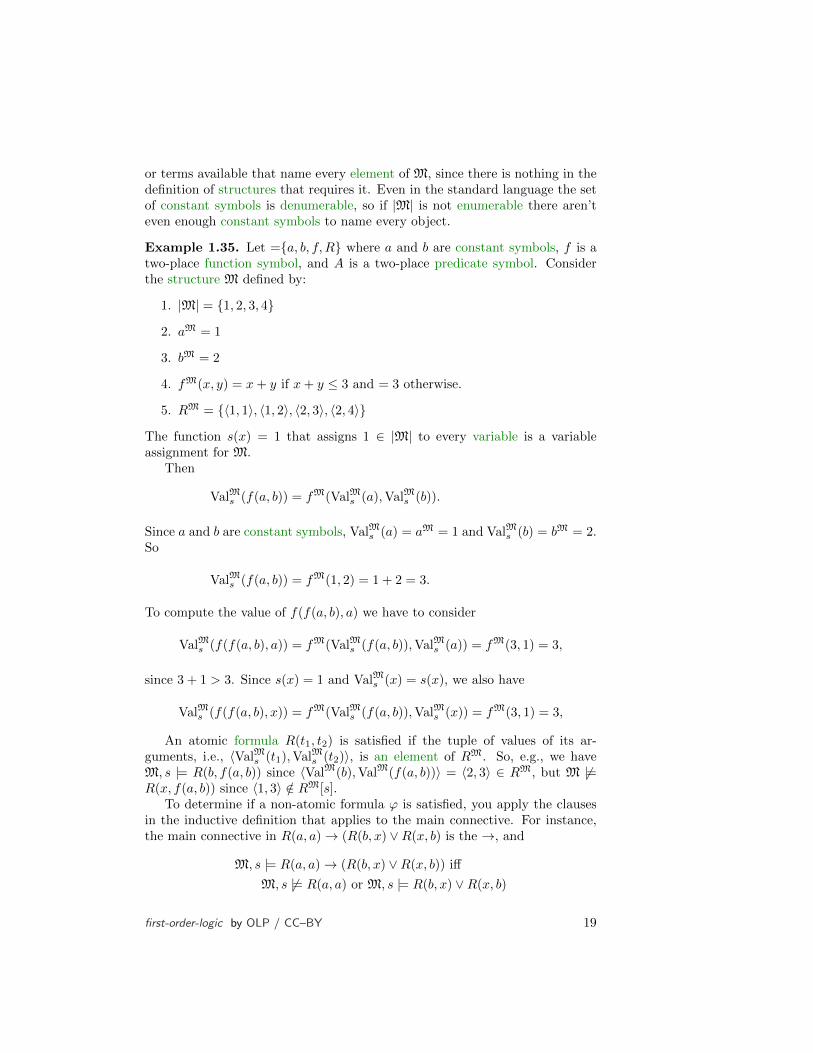
or terms available that name every element of M, since there is nothing in thedefinition of structures that requires it. Even in the standard language the setof constant symbols is denumerable, so if |M| is not enumerable there aren’teven enough constant symbols to name every object.

Example 1.35. Let =a, b, f, R where a and b are constant symbols, f is atwo-place function symbol, and A is a two-place predicate symbol. Considerthe structure M defined by:

1. |M| = 1, 2, 3, 4

2. aM = 1

3. bM = 2

4. fM(x, y) = x+ y if x+ y ≤ 3 and = 3 otherwise.

5. RM = 〈1, 1〉, 〈1, 2〉, 〈2, 3〉, 〈2, 4〉

The function s(x) = 1 that assigns 1 ∈ |M| to every variable is a variableassignment for M.

Then

ValMs (f(a, b)) = fM(ValMs (a),ValMs (b)).

Since a and b are constant symbols, ValMs (a) = aM = 1 and ValMs (b) = bM = 2.So

ValMs (f(a, b)) = fM(1, 2) = 1 + 2 = 3.

To compute the value of f(f(a, b), a) we have to consider

ValMs (f(f(a, b), a)) = fM(ValMs (f(a, b)),ValMs (a)) = fM(3, 1) = 3,

since 3 + 1 > 3. Since s(x) = 1 and ValMs (x) = s(x), we also have

ValMs (f(f(a, b), x)) = fM(ValMs (f(a, b)),ValMs (x)) = fM(3, 1) = 3,

An atomic formula R(t1, t2) is satisfied if the tuple of values of its ar-guments, i.e., 〈ValMs (t1),ValMs (t2)〉, is an element of RM. So, e.g., we haveM, s |= R(b, f(a, b)) since 〈ValM(b),ValM(f(a, b))〉 = 〈2, 3〉 ∈ RM, but M 6|=R(x, f(a, b)) since 〈1, 3〉 /∈ RM[s].

To determine if a non-atomic formula ϕ is satisfied, you apply the clausesin the inductive definition that applies to the main connective. For instance,the main connective in R(a, a)→ (R(b, x) ∨R(x, b) is the →, and

M, s |= R(a, a)→ (R(b, x) ∨R(x, b)) iff

M, s 6|= R(a, a) or M, s |= R(b, x) ∨R(x, b)





Since M, s |= R(a, a) (because 〈1, 1〉 ∈ RM) we can’t yet determine the answerand must first figure out if M, s |= R(b, x) ∨R(x, b):

M, s |= R(b, x) ∨R(x, b) iff

M, s |= R(b, x) or M, s |= R(x, b)

And this is the case, since M, s |= R(x, b) (because 〈1, 2〉 ∈ RM).

Recall that an x-variant of s is a variable assignment that differs from s atmost in what it assigns to x. For every element of |M|, there is an x-variantof s: s1(x) = 1, s2(x) = 2, s3(x) = 3, s4(s) = 4, and with si(y) = s(y) = 1for all variables y other than x are all the x-variants of s for the structure M.Note, in particular, that s1 = s is also an x-variant of s, i.e., s is an x-variantof itself.

To determine if an existentially quantified formula ∃xϕ(x) is satisfied, wehave to determine if M, s′ |= ϕ(x) for at least one x-variant s′ of s. So,

M, s |= ∃x (R(b, x) ∨R(x, b)),

since M, s1 |= R(b, x) ∨R(x, b) (s3 would also fit the bill). But,

M, s 6|= ∃x (R(b, x) ∧R(x, b))

since for none of the si, M, si |= R(b, x) ∧R(x, b).To determine if a universally quantified formula ∀xϕ(x) is satisfied, we have

to determine if M, s′ |= ϕ(x) for all x-variants s′ of s. So,

M, s |= ∀x (R(x, a)→ R(a, x)),

since M, si |= R(x, a)→ R(a, x) for all si (M, s1 |= R(a, x) and M, sj 6|= R(a, x)for j = 2, 3, and 4). But,

M, s 6|= ∀x (R(a, x)→ R(x, a))

since M, s2 6|= R(a, x) → R(x, a) (because M, s2 |= R(a, x) and M, s2 6|=R(x, a)).

For a more complicated case, consider

∀x (R(a, x)→ ∃y R(x, y)).

Since M, s3 6|= R(a, x) and M, s4 6|= R(a, x), the interesting cases where wehave to worry about the consequent of the conditional are only s1 and s2. DoesM, s1 |= ∃y R(x, y) hold? It does if there is at least one y-variant s′1 of s1 sothat M, s′1 |= R(x, y). In fact, s1 is such a y-variant (s1(x) = 1, s1(y) = 1, and〈1, 1〉 ∈ RM), so the answer is yes. To determine if M, s2 |= ∃y R(x, y) we haveto look at the y-variants of s2. Here, s2 itself does not satisfy R(x, y) (s2(x) = 2,





s2(y) = 1, and 〈2, 1〉 /∈ RM). However, consider s′2 ∼y s2 with s′2(y) = 3.M, s′2 |= R(x, y) since 〈2, 3〉 ∈ RM, and so M, s2 |= ∃y R(x, y). In sum, forevery x-variant si of s, either M, si 6|= R(a, x) (i = 3, 4) or M, si |= ∃y R(x, y)(i = 1, 2), and so

M, s |= ∀x (R(a, x)→ ∃y R(x, y)).

On the other hand,

M, s 6|= ∃x (R(a, x) ∧ ∀y R(x, y)).

The only x-variants si of s with M, si |= R(a, x) are s1 and s2. But for each,there is in turn a y-variant s′i ∼y si with s′i(y) = 4 so that M, s′i 6|= R(x, y) andso M, si 6|= ∀y R(x, y) for i = 1, 2. In sum, none of the x-variants si ∼x s aresuch that M, si |= R(a, x) ∧ ∀y R(x, y).

Problem 1.5. Let L = c, f, A with one constant symbol, one one-placefunction symbol and one two-place predicate symbol, and let the structure Mbe given by

1. |M| = 1, 2, 3

2. cM = 3

3. fM(1) = 2, fM(2) = 3, fM(3) = 2

4. AM = 〈1, 2〉, 〈2, 3〉, 〈3, 3〉

(a) Let s(v) = 1 for all variables v. Find out whether

M, s |= ∃x (A(f(z), c)→ ∀y (A(y, x) ∨A(f(y), x)))

Explain why or why not.(b) Give a different structure and variable assignment in which the formula

is not satisfied.

1.12 Variable Assignments

fol:syn:ass:sec

explanationA variable assignment s provides a value for every variable—and there areinfinitely many of them. This is of course not necessary. We require variableassignments to assign values to all variables simply because it makes things alot easier. The value of a term t, and whether or not a formula ϕ is satisfied ina structure with respect to s, only depend on the assignments s makes to thevariables in t and the free variables of ϕ. This is the content of the next twopropositions. To make the idea of “depends on” precise, we show that any twovariable assignments that agree on all the variables in t give the same value,and that ϕ is satisfied relative to one iff it is satisfied relative to the other iftwo variable assignments agree on all free variables of ϕ.

Proposition 1.36.fol:syn:ass:

prop:valindep

If the variables in a term t are among x1, . . . , xn, and

s1(xi) = s2(xi) for i = 1, . . . , n, then ValMs1 (t) = ValMs2 (t).





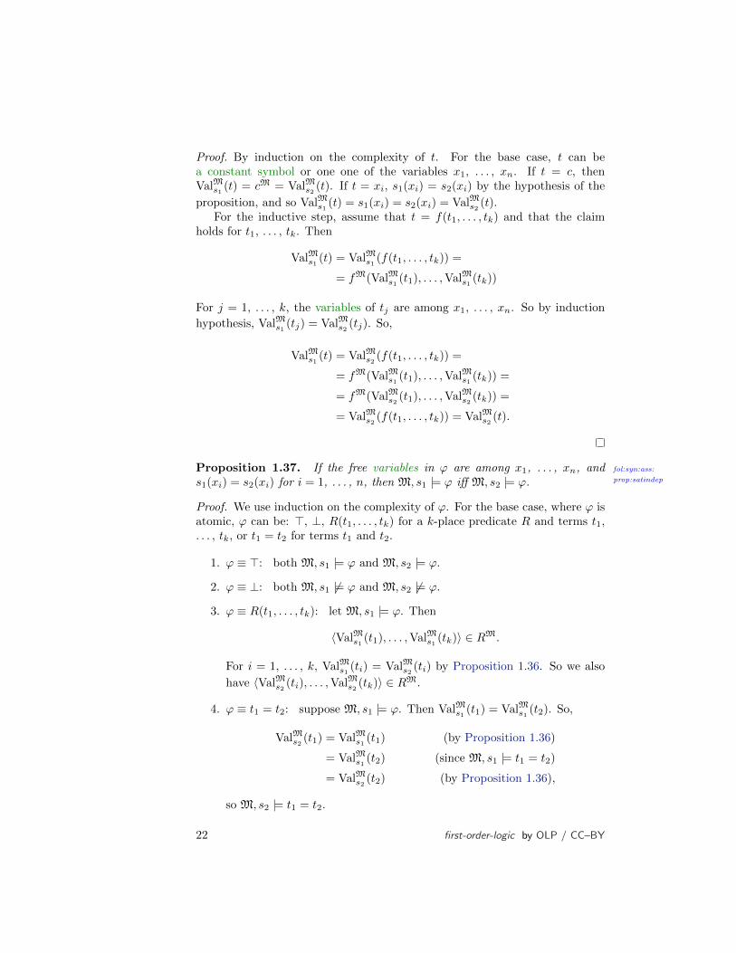
Proof. By induction on the complexity of t. For the base case, t can bea constant symbol or one one of the variables x1, . . . , xn. If t = c, thenValMs1 (t) = cM = ValMs2 (t). If t = xi, s1(xi) = s2(xi) by the hypothesis of the

proposition, and so ValMs1 (t) = s1(xi) = s2(xi) = ValMs2 (t).For the inductive step, assume that t = f(t1, . . . , tk) and that the claim

holds for t1, . . . , tk. Then

ValMs1 (t) = ValMs1 (f(t1, . . . , tk)) =

= fM(ValMs1 (t1), . . . ,ValMs1 (tk))

For j = 1, . . . , k, the variables of tj are among x1, . . . , xn. So by induction

hypothesis, ValMs1 (tj) = ValMs2 (tj). So,

ValMs1 (t) = ValMs2 (f(t1, . . . , tk)) =

= fM(ValMs1 (t1), . . . ,ValMs1 (tk)) =

= fM(ValMs2 (t1), . . . ,ValMs2 (tk)) =

= ValMs2 (f(t1, . . . , tk)) = ValMs2 (t).

Proposition 1.37. fol:syn:ass:

prop:satindep

If the free variables in ϕ are among x1, . . . , xn, ands1(xi) = s2(xi) for i = 1, . . . , n, then M, s1 |= ϕ iff M, s2 |= ϕ.

Proof. We use induction on the complexity of ϕ. For the base case, where ϕ isatomic, ϕ can be: >, ⊥, R(t1, . . . , tk) for a k-place predicate R and terms t1,. . . , tk, or t1 = t2 for terms t1 and t2.

1. ϕ ≡ >: both M, s1 |= ϕ and M, s2 |= ϕ.

2. ϕ ≡ ⊥: both M, s1 6|= ϕ and M, s2 6|= ϕ.

3. ϕ ≡ R(t1, . . . , tk): let M, s1 |= ϕ. Then

〈ValMs1 (t1), . . . ,ValMs1 (tk)〉 ∈ RM.

For i = 1, . . . , k, ValMs1 (ti) = ValMs2 (ti) by Proposition 1.36. So we also

have 〈ValMs2 (ti), . . . ,ValMs2 (tk)〉 ∈ RM.

4. ϕ ≡ t1 = t2: suppose M, s1 |= ϕ. Then ValMs1 (t1) = ValMs1 (t2). So,

ValMs2 (t1) = ValMs1 (t1) (by Proposition 1.36)

= ValMs1 (t2) (since M, s1 |= t1 = t2)

= ValMs2 (t2) (by Proposition 1.36),

so M, s2 |= t1 = t2.





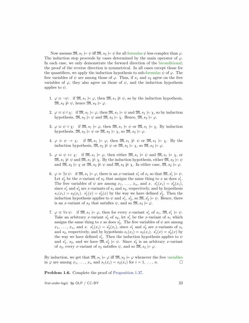
Now assume M, s1 |= ψ iff M, s2 |= ψ for all formulas ψ less complex than ϕ.The induction step proceeds by cases determined by the main operator of ϕ.In each case, we only demonstrate the forward direction of the biconditional;the proof of the reverse direction is symmetrical. In all cases except those forthe quantifiers, we apply the induction hypothesis to sub-formulas ψ of ϕ. Thefree variables of ψ are among those of ϕ. Thus, if s1 and s2 agree on the freevariables of ϕ, they also agree on those of ψ, and the induction hypothesisapplies to ψ.

1. ϕ ≡ ¬ψ: if M, s1 |= ϕ, then M, s1 6|= ψ, so by the induction hypothesis,M, s2 6|= ψ, hence M, s2 |= ϕ.

2. ϕ ≡ ψ∧χ: if M, s1 |= ϕ, then M, s1 |= ψ and M, s1 |= χ, so by inductionhypothesis, M, s2 |= ψ and M, s2 |= χ. Hence, M, s2 |= ϕ.

3. ϕ ≡ ψ ∨ χ: if M, s1 |= ϕ, then M, s1 |= ψ or M, s1 |= χ. By inductionhypothesis, M, s2 |= ψ or M, s2 |= χ, so M, s2 |= ϕ.

4. ϕ ≡ ψ → χ: if M, s1 |= ϕ, then M, s1 6|= ψ or M, s1 |= χ. By theinduction hypothesis, M, s2 6|= ψ or M, s2 |= χ, so M, s2 |= ϕ.

5. ϕ ≡ ψ ↔ χ: if M, s1 |= ϕ, then either M, s1 |= ψ and M, s1 |= χ, orM, s1 6|= ψ and M, s1 6|= χ. By the induction hypothesis, either M, s2 |= ψand M, s2 |= χ or M, s2 6|= ψ and M, s2 6|= χ. In either case, M, s2 |= ϕ.

6. ϕ ≡ ∃xψ: if M, s1 |= ϕ, there is an x-variant s′1 of s1 so that M, s′1 |= ψ.Let s′2 be the x-variant of s2 that assigns the same thing to x as does s′1.The free variables of ψ are among x1, . . . , xn, and x. s′1(xi) = s′2(xi),since s′1 and s′2 are x-variants of s1 and s2, respectively, and by hypothesiss1(xi) = s2(xi). s

′1(x) = s′2(x) by the way we have defined s′2. Then the

induction hypothesis applies to ψ and s′1, s′2, so M, s′2 |= ψ. Hence, thereis an x-variant of s2 that satisfies ψ, and so M, s2 |= ϕ.

7. ϕ ≡ ∀xψ: if M, s1 |= ϕ, then for every x-variant s′1 of s1, M, s′1 |= ψ.Take an arbitrary x-variant s′2 of s2, let s′1 be the x-variant of s1 whichassigns the same thing to x as does s′2. The free variables of ψ are amongx1, . . . , xn, and x. s′1(xi) = s′2(xi), since s′1 and s′2 are x-variants of s1and s2, respectively, and by hypothesis s1(xi) = s2(xi). s

′1(x) = s′2(x) by

the way we have defined s′1. Then the induction hypothesis applies to ψand s′1, s2, and we have M, s′2 |= ψ. Since s′2 is an arbitrary x-variantof s2, every x-variant of s2 satisfies ψ, and so M, s2 |= ϕ.

By induction, we get that M, s1 |= ϕ iff M, s2 |= ϕ whenever the free variablesin ϕ are among x1, . . . , xn and s1(xi) = s2(xi) for i = 1, . . . , n.

Problem 1.6. Complete the proof of Proposition 1.37.





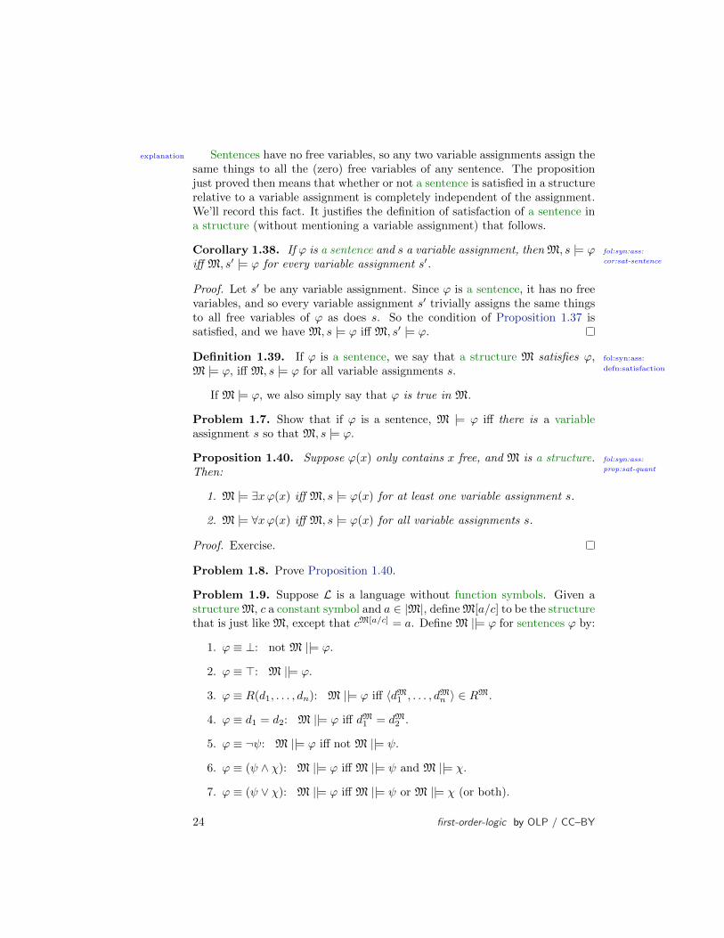
explanation Sentences have no free variables, so any two variable assignments assign thesame things to all the (zero) free variables of any sentence. The propositionjust proved then means that whether or not a sentence is satisfied in a structurerelative to a variable assignment is completely independent of the assignment.We’ll record this fact. It justifies the definition of satisfaction of a sentence ina structure (without mentioning a variable assignment) that follows.

Corollary 1.38. fol:syn:ass:

cor:sat-sentence

If ϕ is a sentence and s a variable assignment, then M, s |= ϕiff M, s′ |= ϕ for every variable assignment s′.

Proof. Let s′ be any variable assignment. Since ϕ is a sentence, it has no freevariables, and so every variable assignment s′ trivially assigns the same thingsto all free variables of ϕ as does s. So the condition of Proposition 1.37 issatisfied, and we have M, s |= ϕ iff M, s′ |= ϕ.

Definition 1.39. fol:syn:ass:

defn:satisfaction

If ϕ is a sentence, we say that a structure M satisfies ϕ,M |= ϕ, iff M, s |= ϕ for all variable assignments s.

If M |= ϕ, we also simply say that ϕ is true in M.

Problem 1.7. Show that if ϕ is a sentence, M |= ϕ iff there is a variableassignment s so that M, s |= ϕ.

Proposition 1.40. fol:syn:ass:

prop:sat-quant

Suppose ϕ(x) only contains x free, and M is a structure.Then:

1. M |= ∃xϕ(x) iff M, s |= ϕ(x) for at least one variable assignment s.

2. M |= ∀xϕ(x) iff M, s |= ϕ(x) for all variable assignments s.

Proof. Exercise.

Problem 1.8. Prove Proposition 1.40.

Problem 1.9. Suppose L is a language without function symbols. Given astructure M, c a constant symbol and a ∈ |M|, define M[a/c] to be the structurethat is just like M, except that cM[a/c] = a. Define M ||= ϕ for sentences ϕ by:

1. ϕ ≡ ⊥: not M ||= ϕ.

2. ϕ ≡ >: M ||= ϕ.

3. ϕ ≡ R(d1, . . . , dn): M ||= ϕ iff 〈dM1 , . . . , dMn 〉 ∈ RM.

4. ϕ ≡ d1 = d2: M ||= ϕ iff dM1 = dM2 .

5. ϕ ≡ ¬ψ: M ||= ϕ iff not M ||= ψ.

6. ϕ ≡ (ψ ∧ χ): M ||= ϕ iff M ||= ψ and M ||= χ.

7. ϕ ≡ (ψ ∨ χ): M ||= ϕ iff M ||= ψ or M ||= χ (or both).





8. ϕ ≡ (ψ → χ): M ||= ϕ iff not M ||= ψ or M ||= χ (or both).

9. ϕ ≡ (ψ ↔ χ): M ||= ϕ iff either both M ||= ψ and M ||= χ, or neitherM ||= ψ nor M ||= χ.

10. ϕ ≡ ∀xψ: M ||= ϕ iff for all a ∈ |M|, M[a/c] ||= ψ[c/x], if c does notoccur in ψ.

11. ϕ ≡ ∃xψ: M ||= ϕ iff there is an a ∈ |M| such that M[a/c] ||= ψ[c/x],if c does not occur in ψ.

Let x1, . . . , xn be all free variables in ϕ, c1, . . . , cn constant symbols not in ϕ,a1, . . . , an ∈ |M|, and s(xi) = ai.

Show that M, s |= ϕ iff M[a1/c1, . . . , an/cn] ||= ϕ[c1/x1] . . . [cn/xn].(This problem shows that it is possible to give a semantics for first-order

logic that makes do without variable assignments.)

Problem 1.10. Suppose that f is a function symbol not in ϕ(x, y). Show thatthere is a structure M such that M |= ∀x ∃y ϕ(x, y) iff there is an M′ such thatM′ |= ∀xϕ(x, f(x)).

(This problem is a special case of what’s known as Skolem’s Theorem;∀xϕ(x, f(x)) is called a Skolem normal form of ∀x∃y ϕ(x, y).)

1.13 Extensionality

fol:syn:ext:sec

explanationExtensionality, sometimes called relevance, can be expressed informally asfollows: the only thing that bears upon the satisfaction of formula ϕ in astructure M relative to a variable assignment s, are the assignments madeby M and s to the elements of the language that actually appear in ϕ.

One immediate consequence of extensionality is that where two structures Mand M′ agree on all the elements of the language appearing in a sentence ϕand have the same domain, M and M′ must also agree on whether or not ϕitself is true.

Proposition 1.41 (Extensionality).fol:syn:ext:

prop:extensionality

Let ϕ be a formula, and M1 and M2 bestructures with |M1| = |M2|, and s a variable assignment on |M1| = |M2|.If cM1 = cM2 , RM1 = RM2 , and fM1 = fM2 for every constant symbol c,relation symbol R, and function symbol f occurring in ϕ, then M1, s |= ϕ iffM2, s |= ϕ.

Proof. First prove (by induction on t) that for every term, ValM1s (t) = ValM2

s (t).Then prove the proposition by induction on ϕ, making use of the claim justproved for the induction basis (where ϕ is atomic).

Problem 1.11. Carry out the proof of Proposition 1.41 in detail.

Corollary 1.42 (Extensionality).fol:syn:ext:

cor:extensionality-sent

Let ϕ be a sentence and M1, M2 as inProposition 1.41. Then M1 |= ϕ iff M2 |= ϕ.





Proof. Follows from Proposition 1.41 by Corollary 1.38.

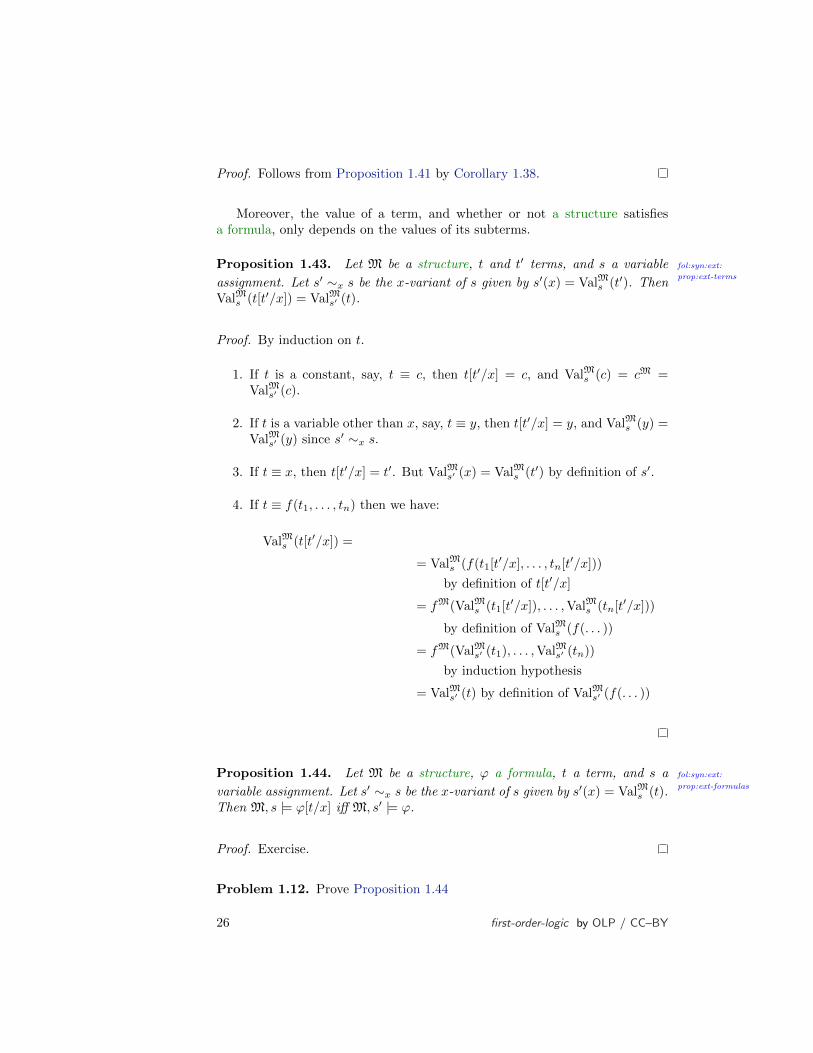
Moreover, the value of a term, and whether or not a structure satisfiesa formula, only depends on the values of its subterms.

Proposition 1.43. fol:syn:ext:

prop:ext-terms

Let M be a structure, t and t′ terms, and s a variable

assignment. Let s′ ∼x s be the x-variant of s given by s′(x) = ValMs (t′). ThenValMs (t[t′/x]) = ValMs′ (t).

Proof. By induction on t.

1. If t is a constant, say, t ≡ c, then t[t′/x] = c, and ValMs (c) = cM =ValMs′ (c).

2. If t is a variable other than x, say, t ≡ y, then t[t′/x] = y, and ValMs (y) =ValMs′ (y) since s′ ∼x s.

3. If t ≡ x, then t[t′/x] = t′. But ValMs′ (x) = ValMs (t′) by definition of s′.

4. If t ≡ f(t1, . . . , tn) then we have:

ValMs (t[t′/x]) =

= ValMs (f(t1[t′/x], . . . , tn[t′/x]))

by definition of t[t′/x]

= fM(ValMs (t1[t′/x]), . . . ,ValMs (tn[t′/x]))

by definition of ValMs (f(. . . ))

= fM(ValMs′ (t1), . . . ,ValMs′ (tn))

by induction hypothesis

= ValMs′ (t) by definition of ValMs′ (f(. . . ))

Proposition 1.44. fol:syn:ext:

prop:ext-formulas

Let M be a structure, ϕ a formula, t a term, and s a

variable assignment. Let s′ ∼x s be the x-variant of s given by s′(x) = ValMs (t).Then M, s |= ϕ[t/x] iff M, s′ |= ϕ.

Proof. Exercise.

Problem 1.12. Prove Proposition 1.44





1.14 Semantic Notions

fol:syn:sem:sec

explanationGive the definition of structures for first-order languages, we can definesome basic semantic properties of and relationships between sentences. Thesimplest of these is the notion of validity of a sentence. A sentence is valid ifit is satisfied in every structure. Valid sentences are those that are satisfiedregardless of how the non-logical symbols in it are interpreted. Valid sentencesare therefore also called logical truths—they are true, i.e., satisfied, in anystructure and hence their truth depends only on the logical symbols occurringin them and their syntactic structure, but not on the non-logical symbols ortheir interpretation.

Definition 1.45 (Validity). A sentence ϕ is valid, ϕ, iff M |= ϕ for everystructure M.

Definition 1.46 (Entailment). A set of sentences Γ entails a sentence ϕ,Γ ϕ, iff for every structure M with M |= Γ , M |= ϕ.

Definition 1.47 (Satisfiability). A set of sentences Γ is satisfiable if M |= Γfor some structure M. If Γ is not satisfiable it is called unsatisfiable.

Proposition 1.48. A sentence ϕ is valid iff Γ ϕ for every set of sentences Γ .

Proof. For the forward direction, let ϕ be valid, and let Γ be a set of sentences.Let M be a structure so that M |= Γ . Since ϕ is valid, M |= ϕ, hence Γ ϕ.

For the contrapositive of the reverse direction, let ϕ be invalid, so there isa structure M with M 6|= ϕ. When Γ = >, since > is valid, M |= Γ . Hence,there is a structure M so that M |= Γ but M 6|= ϕ, hence Γ does not entailϕ.

Proposition 1.49.fol:syn:sem:

prop:entails-unsat

Γ ϕ iff Γ ∪ ¬ϕ is unsatisfiable.

Proof. For the forward direction, suppose Γ ϕ and suppose to the contrarythat there is a structure M so that M |= Γ ∪ ¬ϕ. Since M |= Γ and Γ ϕ,M |= ϕ. Also, since M |= Γ ∪ ¬ϕ, M |= ¬ϕ, so we have both M |= ϕ andM 6|= ϕ, a contradiction. Hence, there can be no such structure M, so Γ ∪ ϕis unsatisfiable.

For the reverse direction, suppose Γ ∪ ¬ϕ is unsatisfiable. So for everystructure M, either M 6|= Γ or M |= ϕ. Hence, for every structure M withM |= Γ , M |= ϕ, so Γ ϕ.

Problem 1.13. 1. Show that Γ ⊥ iff Γ is unsatisfiable.

2. Show that Γ ∪ ϕ ⊥ iff Γ ¬ϕ.

3. Suppose c does not occur in ϕ or Γ . Show that Γ ∀xϕ iff Γ ϕ[c/x].

Proposition 1.50. If Γ ⊆ Γ ′ and Γ ϕ, then Γ ′ ϕ.





Chapter 2

Theories and Their Models

2.1 Introduction

fol:mat:int:sec

explanationThe development of the axiomatic method is a significant achievement in thehistory of science, and is of special importance in the history of mathematics.An axiomatic development of a field involves the clarification of many questions:What is the field about? What are the most fundamental concepts? How arethey related? Can all the concepts of the field be defined in terms of thesefundamental concepts? What laws do, and must, these concepts obey?

The axiomatic method and logic were made for each other. Formal logicprovides the tools for formulating axiomatic theories, for proving theoremsfrom the axioms of the theory in a precisely specified way, for studying theproperties of all systems satisfying the axioms in a systematic way.

Definition 2.1. A set of sentences Γ is closed iff, whenever Γ ϕ then ϕ ∈ Γ .The closure of a set of sentences Γ is ϕ : Γ ϕ.

We say that Γ is axiomatized by a set of sentences ∆ if Γ is the closureof ∆

explanationWe can think of an axiomatic theory as the set of sentences that is ax-iomatized by its set of axioms ∆. In other words, when we have a first-orderlanguage which contains non-logical symbols for the primitives of the axiomat-ically developed science we wish to study, together with a set of sentencesthat express the fundamental laws of the science, we can think of the theoryas represented by all the sentences in this language that are entailed by theaxioms. This ranges from simple examples with only a single primitive andsimple axioms, such as the theory of partial orders, to complex theories suchas Newtonian mechanics.

The important logical facts that make this formal approach to the axiomaticmethod so important are the following. Suppose Γ is an axiom system for atheory, i.e., a set of sentences.

1. We can state precisely when an axiom system captures an intended classof structures. That is, if we are interested in a certain class of struc-

29

tures, we will successfully capture that class by an axiom system Γ iffthe structures are exactly those M such that M |= Γ .

2. We may fail in this respect because there are M such that M |= Γ , butM is not one of the structures we intend. This may lead us to add axiomswhich are not true in M.

3. If we are successful at least in the respect that Γ is true in all the intendedstructures, then a sentence ϕ is true in all intended structures wheneverΓ ϕ. Thus we can use logical tools (such as proof methods) to showthat sentences are true in all intended structures simply by showing thatthey are entailed by the axioms.

4. Sometimes we don’t have intended structures in mind, but instead startfrom the axioms themselves: we begin with some primitives that wewant to satisfy certain laws which we codify in an axiom system. Onething that we would like to verify right away is that the axioms do notcontradict each other: if they do, there can be no concepts that obeythese laws, and we have tried to set up an incoherent theory. We canverify that this doesn’t happen by finding a model of Γ . And if thereare models of our theory, we can use logical methods to investigate them,and we can also use logical methods to construct models.

5. The independence of the axioms is likewise an important question. It mayhappen that one of the axioms is actually a consequence of the others,and so is redundant. We can prove that an axiom ϕ in Γ is redundant byproving Γ \ ϕ ϕ. We can also prove that an axiom is not redundantby showing that (Γ \ϕ)∪¬ϕ is satisfiable. For instance, this is how itwas shown that the parallel postulate is independent of the other axiomsof geometry.

6. Another important question is that of definability of concepts in a theory:The choice of the language determines what the models of a theory con-sists of. But not every aspect of a theory must be represented separatelyin its models. For instance, every ordering ≤ determines a correspondingstrict ordering <—given one, we can define the other. So it is not neces-sary that a model of a theory involving such an order must also containthe corresponding strict ordering. When is it the case, in general, thatone relation can be defined in terms of others? When is it impossible todefine a relation in terms of other (and hence must add it to the primitivesof the language)?

2.2 Expressing Properties of Structures

fol:mat:exs:sec

explanation It is often useful and important to express conditions on functions and rela-tions, or more generally, that the functions and relations in a structure satisfythese conditions. For instance, we would like to have ways of distinguishing





those structures for a language which “capture” what we want the predicatesymbols to “mean” from those that do not. Of course we’re completely freeto specify which structures we “intend,” e.g., we can specify that the inter-pretation of the predicate symbol ≤ must be an ordering, or that we are onlyinterested in interpretations of L in which the domain consists of sets and ∈ isinterpreted by the “is an element of” relation. But can we do this with sen-tences of the language? In other words, which conditions on a structure M canwe express by a sentence (or perhaps a set of sentences) in the language of M?There are some conditions that we will not be able to express. For instance,there is no sentence of LA which is only true in a structure M if |M| = N.We cannot express “the domain contains only natural numbers.” But thereare “structural properties” of structures that we perhaps can express. Whichproperties of structures can we express by sentences? Or, to put it another way,which collections of structures can we describe as those making a sentence (orset of sentences) true?

Definition 2.2 (Model of a set). Let Γ be a set of sentences in a language L.We say that a structure M is a model of Γ if M |= ϕ for all ϕ ∈ Γ .

Example 2.3. The sentence ∀xx ≤ x is true in M iff ≤M is a reflexive relation.The sentence ∀x∀y ((x ≤ y ∧ y ≤ x) → x = y) is true in M iff ≤M is anti-symmetric. The sentence ∀x∀y ∀z ((x ≤ y ∧ y ≤ z) → x ≤ z) is true in M iff≤M is transitive. Thus, the models of

∀xx ≤ x,∀x∀y ((x ≤ y ∧ y ≤ x)→ x = y),

∀x∀y ∀z ((x ≤ y ∧ y ≤ z)→ x ≤ z)

are exactly those structures in which ≤M is reflexive, anti-symmetric, andtransitive, i.e., a partial order. Hence, we can take them as axioms for thefirst-order theory of partial orders.

2.3 Examples of First-Order Theories

fol:mat:the:sec

Example 2.4. The theory of strict linear orders in the language L< is axiom-atized by the set

∀x¬x < x,

∀x∀y ((x < y ∨ y < x) ∨ x = y),

∀x∀y ∀z ((x < y ∧ y < z)→ x < z)

It completely captures the intended structures: every strict linear order is amodel of this axiom system, and vice versa, if R is a linear order on a set X,then the structure M with |M| = X and <M = R is a model of this theory.





Example 2.5. The theory of groups in the language (constant symbol), ·(two-place function symbol) is axiomatized by

∀x (x · ) = x

∀x∀y ∀z (x · (y · z)) = ((x · y) · z)∀x∃y (x · y) =

Example 2.6. The theory of Peano arithmetic is axiomatized by the followingsentences in the language of arithmetic LA.

¬∃xx′ =

∀x ∀y (x′ = y′ → x = y)

∀x ∀y (x < y ↔ ∃z (x+ z′ = y))

∀x (x+ ) = x

∀x∀y (x+ y′) = (x+ y)′

∀x (x× ) =

∀x∀y (x× y′) = ((x× y) + x)

plus all sentences of the form

(ϕ() ∧ ∀x (ϕ(x)→ ϕ(x′)))→ ∀xϕ(x)

Since there are infinitely many sentences of the latter form, this axiom systemis infinite. The latter form is called the induction schema. (Actually, theinduction schema is a bit more complicated than we let on here.)

The third axiom is an explicit definition of <.

Example 2.7. The theory of pure sets plays an important role in the founda-tions (and in the philosophy) of mathematics. A set is pure if all its elementsare also pure sets. The empty set counts therefore as pure, but a set that hassomething as an element that is not a set would not be pure. So the pure setsare those that are formed just from the empty set and no “urelements,” i.e.,objects that are not themselves sets.

The following might be considered as an axiom system for a theory of puresets:

∃x¬∃y y ∈ x∀x ∀y (∀z(z ∈ x↔ z ∈ y)→ x = y)

∀x∀y ∃z ∀u (u ∈ z ↔ (u = x ∨ u = y))

∀x∃y ∀z (z ∈ y ↔ ∃u (z ∈ u ∧ u ∈ x))

plus all sentences of the form

∃x∀y (y ∈ x↔ ϕ(y))





The first axiom says that there is a set with no elements (i.e., ∅ exists); thesecond says that sets are extensional; the third that for any sets X and Y , theset X,Y exists; the fourth that for any sets X and Y , the set X ∪ Y exists.

The sentences mentioned last are collectively called the naive comprehen-sion scheme. It essentially says that for every ϕ(x), the set x : ϕ(x) exists—soat first glance a true, useful, and perhaps even necessary axiom. It is called“naive” because, as it turns out, it makes this theory unsatisfiable: if you takeϕ(y) to be ¬y ∈ y, you get the sentence

∃x ∀y (y ∈ x↔ ¬y ∈ y)

and this sentence is not satisfied in any structure.

Example 2.8. In the area of mereology, the relation of parthood is a funda-mental relation. Just like theories of sets, there are theories of parthood thataxiomatize various conceptions (sometimes conflicting) of this relation.

The language of mereology contains a single two-place predicate symbol P ,and P (x, y) “means” that x is a part of y. When we have this interpretationin mind, a structure for this language is called a parthood structure. Of course,not every structure for a single two-place predicate will really deserve thisname. To have a chance of capturing “parthood,” PM must satisfy someconditions, which we can lay down as axioms for a theory of parthood. Forinstance, parthood is a partial order on objects: every object is a part (albeitan improper part) of itself; no two different objects can be parts of each other;a part of a part of an object is itself part of that object. Note that in this sense“is a part of” resembles “is a subset of,” but does not resemble “is an elementof” which is neither reflexive nor transitive.

∀xP (x, x),

∀x∀y ((P (x, y) ∧ P (y, x))→ x = y),

∀x∀y ∀z ((P (x, y) ∧ P (y, z))→ P (x, z)),

Moreover, any two objects have a mereological sum (an object that has thesetwo objects as parts, and is minimal in this respect).

∀x∀y ∃z ∀u (P (z, u)↔ (P (x, u) ∧ P (y, u)))

These are only some of the basic principles of parthood considered by meta-physicians. Further principles, however, quickly become hard to formulate orwrite down without first introducting some defined relations. For instance,most metaphysicians interested in mereology also view the following as a validprinciple: whenever an object x has a proper part y, it also has a part z thathas no parts in common with y, and so that the fusion of y and z is x.

2.4 Expressing Relations in a Structure

fol:mat:exr:sec

explanation





One main use formulas can be put to is to express properties and relationsin a structure M in terms of the primitives of the language L of M. By this wemean the following: the domain of M is a set of objects. The constant symbols,function symbols, and predicate symbols are interpreted in M by some objectsin|M|, functions on |M|, and relations on |M|. For instance, if A20 is in L, then

M assigns to it a relation R = A20M

. Then the formula A20(v1, v2) expressesthat very relation, in the following sense: if a variable assignment s maps v1 toa ∈ |M| and v2 to b ∈ |M|, then

Rab iff M, s |= A20(v1, v2).

Note that we have to involve variable assignments here: we can’t just say “Rabiff M |= A20(a, b)” because a and b are not symbols of our language: they areelements of |M|.

Since we don’t just have atomic formulas, but can combine them using thelogical connectives and the quantifiers, more complex formulas can define otherrelations which aren’t directly built into M. We’re interested in how to do that,and specifically, which relations we can define in a structure.

Definition 2.9. Let ϕ(v1, . . . , vn) be a formula of L in which only v1,. . . ,vn occur free, and let M be a structure for L. ϕ(v1, . . . , vn) expresses therelation R ⊆ |M|n iff

Ra1 . . . an iff M, s |= ϕ(v1, . . . , vn)

for any variable assignment s with s(vi) = ai (i = 1, . . . , n).

Example 2.10. In the standard model of arithmetic N, the formula v1 <v2 ∨ v1 = v2 expresses the ≤ relation on N. The formula v2 = v ′1 expressesthe successor relation, i.e., the relation R ⊆ N2 where Rnm holds if m is thesuccessor of n. The formula v1 = v ′2 expresses the predecessor relation. Theformulas ∃v3 (v3 6= ∧ v2 = (v1 + v3)) and ∃v3 (v1 + v3

′) = v2 both express the< relation. This means that the predicate symbol < is actually superfluous inthe language of arithmetic; it can be defined.

explanation This idea is not just interesting in specific structures, but generally when-ever we use a language to describe an intended model or models, i.e., when weconsider theories. These theories often only contain a few predicate symbols asbasic symbols, but in the domain they are used to describe often many otherrelations play an important role. If these other relations can be systematicallyexpressed by the relations that interpret the basic predicate symbols of thelanguage, we say we can define them in the language.

Problem 2.1. Find formulas in LA which define the following relations:

1. n is between i and j;

2. n evenly divides m (i.e., m is a multiple of n);





3. n is a prime number (i.e., no number other than 1 and n evenly divides n).

Problem 2.2. Suppose the formula ϕ(v1, v2) expresses the relation R ⊆ |M|2in a structure M. Find formulas that express the following relations:

1. the inverse R−1 of R;

2. the relative product R | R;

Can you find a way to express R+, the transitive closure of R?

Problem 2.3. Let L be the language containing a 2-place predicate symbol< only (no other constant symbols, function symbols or predicate symbols—except of course =). Let N be the structure such that |N| = N, and <N =〈n,m〉 : n < m. Prove the following:

1. 0 is definable in N;



4. for each n ∈ N, the set n is definable in N;

5. every finite subset of |N| is definable in N;

6. every co-finite subset of |N| is definable in N (where X ⊆ N is co-finiteiff N \X is finite).

2.5 The Theory of Sets

fol:mat:set:sec

Almost all of mathematics can be developed in the theory of sets. Develop-ing mathematics in this theory involves a number of things. First, it requiresa set of axioms for the relation ∈. A number of different axiom systems havebeen developed, sometimes with conflicting properties of ∈. The axiom systemknown as ZFC, Zermelo-Fraenkel set theory with the axiom of choice standsout: it is by far the most widely used and studied, because it turns out that itsaxioms suffice to prove almost all the things mathematicians expect to be ableto prove. But before that can be established, it first is necessary to make clearhow we can even express all the things mathematicians would like to express.For starters, the language contains no constant symbols or function symbols, soit seems at first glance unclear that we can talk about particular sets (such as∅ or N), can talk about operations on sets (such as X ∪Y and ℘(X)), let aloneother constructions which involve things other than sets, such as relations andfunctions.

To begin with, “is an element of” is not the only relation we are interestedin: “is a subset of” seems almost as important. But we can define “is a subsetof” in terms of “is an element of.” To do this, we have to find a formula ϕ(x, y)in the language of set theory which is satisfied by a pair of sets 〈X,Y 〉 iff





X ⊆ Y . But X is a subset of Y just in case all elements of X are also elementsof Y . So we can define ⊆ by the formula

∀z (z ∈ x→ z ∈ y)

Now, whenever we want to use the relation ⊆ in a formula, we could insteaduse that formula (with x and y suitably replaced, and the bound variable zrenamed if necessary). For instance, extensionality of sets means that if anysets x and y are contained in each other, then x and y must be the same set.This can be expressed by ∀x∀y ((x ⊆ y ∧ y ⊆ x)→ x = y), or, if we replace ⊆by the above definition, by

∀x ∀y ((∀z (z ∈ x→ z ∈ y) ∧ ∀z (z ∈ y → z ∈ x))→ x = y).

This is in fact one of the axioms of ZFC, the “axiom of extensionality.”There is no constant symbol for ∅, but we can express “x is empty” by

¬∃y y ∈ x. Then “∅ exists” becomes the sentence ∃x¬∃y y ∈ x. This isanother axiom of ZFC. (Note that the axiom of extensionality implies thatthere is only one empty set.) Whenever we want to talk about ∅ in the languageof set theory, we would write this as “there is a set that’s empty and . . . ” Asan example, to express the fact that ∅ is a subset of every set, we could write

∃x (¬∃y y ∈ x ∧ ∀z x ⊆ z)

where, of course, x ⊆ z would in turn have to be replaced by its definition.To talk about operations on sets, such has X ∪Y and ℘(X), we have to use

a similar trick. There are no function symbols in the language of set theory,but we can express the functional relations X ∪ Y = Z and ℘(X) = Y by

∀u ((u ∈ x ∨ u ∈ y)↔ u ∈ z)∀u (u ⊆ x↔ u ∈ y)

since the elements of X∪Y are exactly the sets that are either elements of X orelements of Y , and the elements of ℘(X) are exactly the subsets of X. However,this doesn’t allow us to use x∪y or ℘(x) as if they were terms: we can only usethe entire formulas that define the relations X∪Y = Z and ℘(X) = Y . In fact,we do not know that these relations are ever satisfied, i.e., we do not know thatunions and power sets always exist. For instance, the sentence ∀x ∃y ℘(x) = yis another axiom of ZFC (the power set axiom).

Now what about talk of ordered pairs or functions? Here we have to explainhow we can think of ordered pairs and functions as special kinds of sets. Oneway to define the ordered pair 〈x, y〉 is as the set x, x, y. But like before,we cannot introduce a function symbol that names this set; we can only definethe relation 〈x, y〉 = z, i.e., x, x, y = z:

∀u (u ∈ z ↔ (∀v (v ∈ u↔ v = x) ∨ ∀v (v ∈ u↔ (v = x ∨ v = y))))

This says that the elements u of z are exactly those sets which either have xas its only element or have x and y as its only elements (in other words, those





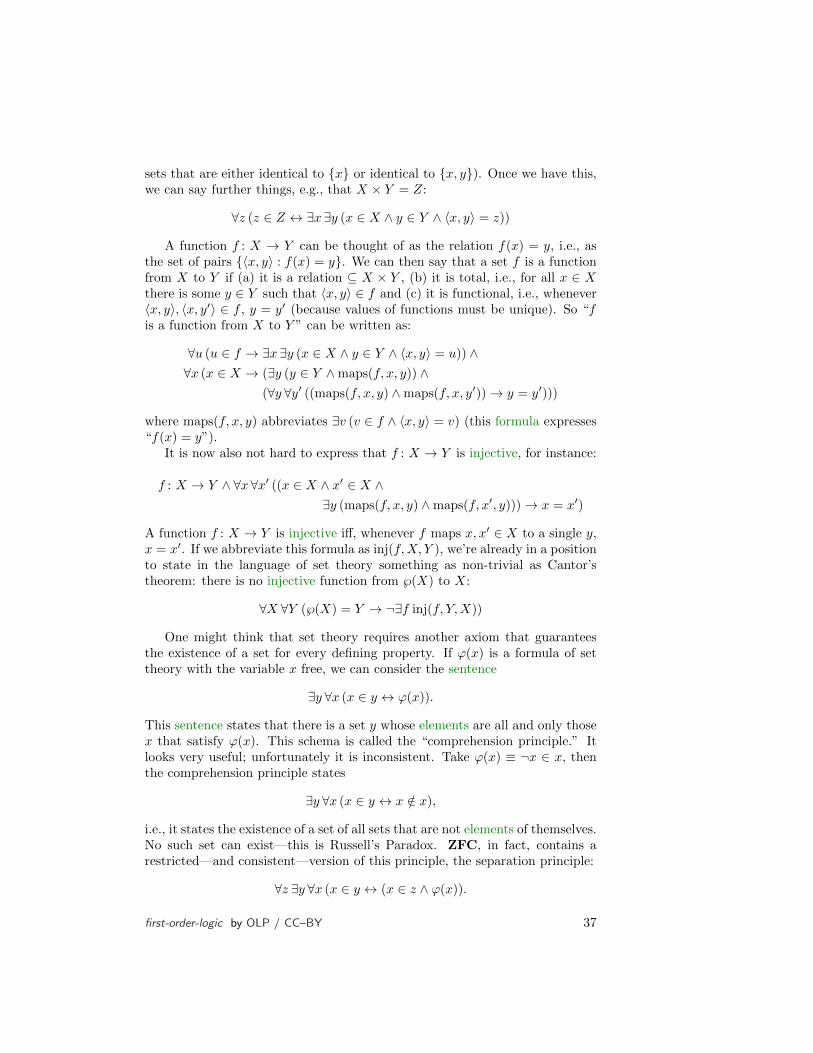
sets that are either identical to x or identical to x, y). Once we have this,we can say further things, e.g., that X × Y = Z:

∀z (z ∈ Z ↔ ∃x∃y (x ∈ X ∧ y ∈ Y ∧ 〈x, y〉 = z))

A function f : X → Y can be thought of as the relation f(x) = y, i.e., asthe set of pairs 〈x, y〉 : f(x) = y. We can then say that a set f is a functionfrom X to Y if (a) it is a relation ⊆ X × Y , (b) it is total, i.e., for all x ∈ Xthere is some y ∈ Y such that 〈x, y〉 ∈ f and (c) it is functional, i.e., whenever〈x, y〉, 〈x, y′〉 ∈ f , y = y′ (because values of functions must be unique). So “fis a function from X to Y ” can be written as:

∀u (u ∈ f → ∃x∃y (x ∈ X ∧ y ∈ Y ∧ 〈x, y〉 = u)) ∧∀x (x ∈ X → (∃y (y ∈ Y ∧maps(f, x, y)) ∧

(∀y ∀y′ ((maps(f, x, y) ∧maps(f, x, y′))→ y = y′)))

where maps(f, x, y) abbreviates ∃v (v ∈ f ∧ 〈x, y〉 = v) (this formula expresses“f(x) = y”).

It is now also not hard to express that f : X → Y is injective, for instance:

f : X → Y ∧ ∀x ∀x′ ((x ∈ X ∧ x′ ∈ X ∧∃y (maps(f, x, y) ∧maps(f, x′, y)))→ x = x′)

A function f : X → Y is injective iff, whenever f maps x, x′ ∈ X to a single y,x = x′. If we abbreviate this formula as inj(f,X, Y ), we’re already in a positionto state in the language of set theory something as non-trivial as Cantor’stheorem: there is no injective function from ℘(X) to X:

∀X ∀Y (℘(X) = Y → ¬∃f inj(f, Y,X))

One might think that set theory requires another axiom that guaranteesthe existence of a set for every defining property. If ϕ(x) is a formula of settheory with the variable x free, we can consider the sentence

∃y ∀x (x ∈ y ↔ ϕ(x)).

This sentence states that there is a set y whose elements are all and only thosex that satisfy ϕ(x). This schema is called the “comprehension principle.” Itlooks very useful; unfortunately it is inconsistent. Take ϕ(x) ≡ ¬x ∈ x, thenthe comprehension principle states

∃y ∀x (x ∈ y ↔ x /∈ x),

i.e., it states the existence of a set of all sets that are not elements of themselves.No such set can exist—this is Russell’s Paradox. ZFC, in fact, contains arestricted—and consistent—version of this principle, the separation principle:

∀z ∃y ∀x (x ∈ y ↔ (x ∈ z ∧ ϕ(x)).





Problem 2.4. Show that the comprehension principle is inconsistent by givinga derivation that shows

∃y ∀x (x ∈ y ↔ x /∈ x) ` ⊥.

It may help to first show (A→ ¬A) ∧ (¬A→ A) ` ⊥.

2.6 Expressing the Size of Structures

fol:mat:siz:sec

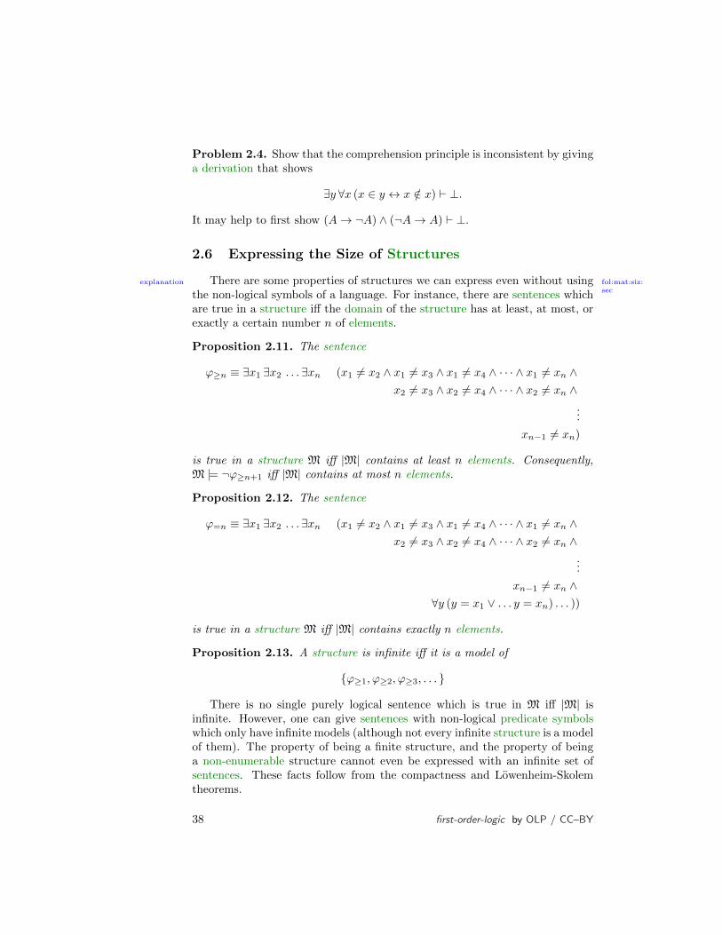
explanation There are some properties of structures we can express even without usingthe non-logical symbols of a language. For instance, there are sentences whichare true in a structure iff the domain of the structure has at least, at most, orexactly a certain number n of elements.

Proposition 2.11. The sentence

ϕ≥n ≡ ∃x1 ∃x2 . . . ∃xn (x1 6= x2 ∧ x1 6= x3 ∧ x1 6= x4 ∧ · · · ∧ x1 6= xn ∧x2 6= x3 ∧ x2 6= x4 ∧ · · · ∧ x2 6= xn ∧

...

xn−1 6= xn)

is true in a structure M iff |M| contains at least n elements. Consequently,M |= ¬ϕ≥n+1 iff |M| contains at most n elements.

Proposition 2.12. The sentence

ϕ=n ≡ ∃x1 ∃x2 . . . ∃xn (x1 6= x2 ∧ x1 6= x3 ∧ x1 6= x4 ∧ · · · ∧ x1 6= xn ∧x2 6= x3 ∧ x2 6= x4 ∧ · · · ∧ x2 6= xn ∧

...

xn−1 6= xn ∧∀y (y = x1 ∨ . . . y = xn) . . . ))

is true in a structure M iff |M| contains exactly n elements.

Proposition 2.13. A structure is infinite iff it is a model of

ϕ≥1, ϕ≥2, ϕ≥3, . . .

There is no single purely logical sentence which is true in M iff |M| isinfinite. However, one can give sentences with non-logical predicate symbolswhich only have infinite models (although not every infinite structure is a modelof them). The property of being a finite structure, and the property of beinga non-enumerable structure cannot even be expressed with an infinite set ofsentences. These facts follow from the compactness and Lowenheim-Skolemtheorems.





Chapter 3

The Sequent Calculus

3.1 Rules and Derivations

fol:seq:rul:sec

Let L be a first-order language with the usual constants, variables, logicalsymbols, and auxiliary symbols (parentheses and the comma).

Definition 3.1 (sequent). A sequent is an expression of the form

Γ ⇒ ∆

where Γ and ∆ are finite (possibly empty) sets of sentences of the language L.The formulas in Γ are the antecedent formulas, while the formulae in ∆ arethe succedent formulas.

The intuitive idea behind a sequent is: if all of the antecedent formulas hold,then at least one of the succedent formulas holds. That is, if Γ = Γ1, . . . , Γmand ∆ = ∆1, . . . ,∆n, then Γ ⇒ ∆ holds iff

(Γ1 ∧ · · · ∧ Γm)→ (∆1 ∨ · · · ∨∆n)

holds.When m = 0, ⇒ ∆ holds iff ∆1 ∨ · · · ∨∆n holds. When n = 0, Γ ⇒

holds iff Γ1 ∧ · · · ∧ Γm does not.

An empty succedent is sometimes filled with the ⊥ symbol. he empty sequent⇒ canonically represents a contradiction.

We write Γ, ϕ (or ϕ, Γ ) for Γ ∪ ϕ, and Γ,∆ for Γ ∪∆.

Definition 3.2 (Inference). An inference is an expression of the form

S1

Sor

S1 S2

S

where S, S1, and S2 are sequents. S1 and S2 are called the upper sequents andS the lower sequent of the inference.

39

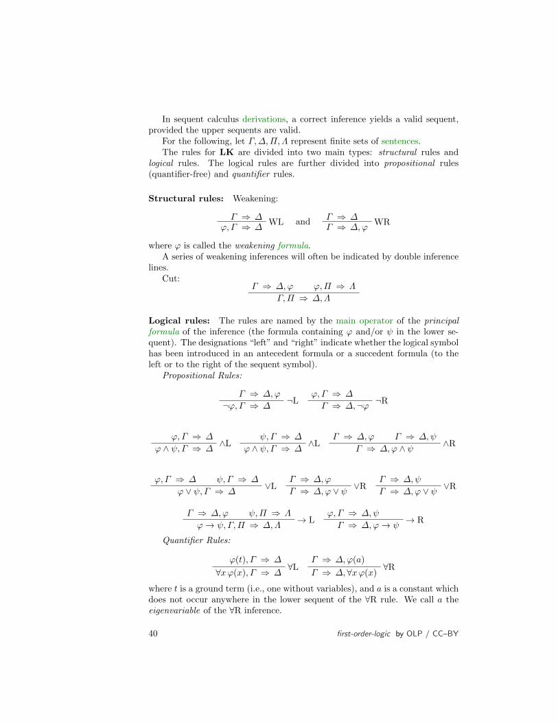
In sequent calculus derivations, a correct inference yields a valid sequent,provided the upper sequents are valid.

For the following, let Γ,∆,Π,Λ represent finite sets of sentences.The rules for LK are divided into two main types: structural rules and

logical rules. The logical rules are further divided into propositional rules(quantifier-free) and quantifier rules.

Structural rules: Weakening:

Γ ⇒ ∆WL

ϕ, Γ ⇒ ∆and

Γ ⇒ ∆WR

Γ ⇒ ∆,ϕ

where ϕ is called the weakening formula.A series of weakening inferences will often be indicated by double inference

lines.Cut:

Γ ⇒ ∆,ϕ ϕ,Π ⇒ Λ

Γ,Π ⇒ ∆,Λ

Logical rules: The rules are named by the main operator of the principalformula of the inference (the formula containing ϕ and/or ψ in the lower se-quent). The designations “left” and “right” indicate whether the logical symbolhas been introduced in an antecedent formula or a succedent formula (to theleft or to the right of the sequent symbol).

Propositional Rules:

Γ ⇒ ∆,ϕ¬L¬ϕ, Γ ⇒ ∆

ϕ,Γ ⇒ ∆¬R

Γ ⇒ ∆,¬ϕ

ϕ, Γ ⇒ ∆∧L

ϕ ∧ ψ, Γ ⇒ ∆

ψ,Γ ⇒ ∆∧L

ϕ ∧ ψ, Γ ⇒ ∆

Γ ⇒ ∆,ϕ Γ ⇒ ∆,ψ∧R

Γ ⇒ ∆,ϕ ∧ ψ

ϕ, Γ ⇒ ∆ ψ,Γ ⇒ ∆∨L

ϕ ∨ ψ, Γ ⇒ ∆

Γ ⇒ ∆,ϕ∨R

Γ ⇒ ∆,ϕ ∨ ψΓ ⇒ ∆,ψ

∨RΓ ⇒ ∆,ϕ ∨ ψ

Γ ⇒ ∆,ϕ ψ,Π ⇒ Λ→ L

ϕ→ ψ, Γ,Π ⇒ ∆,Λ

ϕ, Γ ⇒ ∆,ψ→ R

Γ ⇒ ∆,ϕ→ ψ

Quantifier Rules:

ϕ(t), Γ ⇒ ∆∀L∀xϕ(x), Γ ⇒ ∆

Γ ⇒ ∆,ϕ(a)∀R

Γ ⇒ ∆, ∀xϕ(x)

where t is a ground term (i.e., one without variables), and a is a constant whichdoes not occur anywhere in the lower sequent of the ∀R rule. We call a theeigenvariable of the ∀R inference.





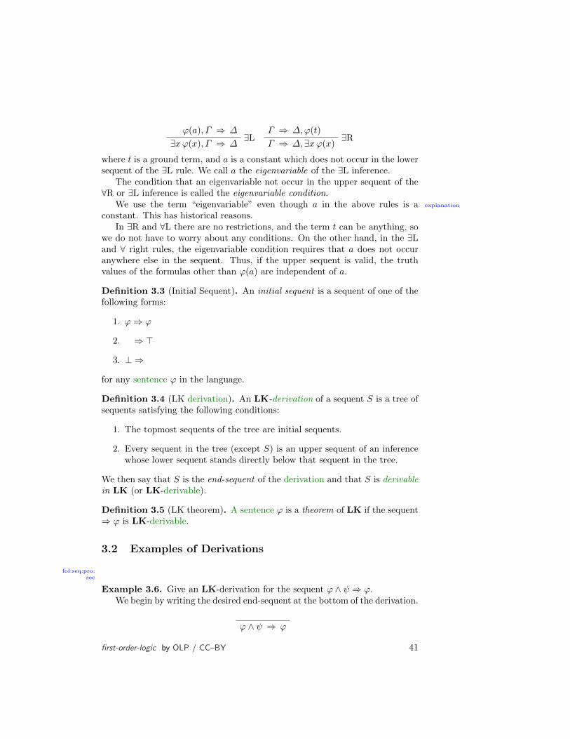
ϕ(a), Γ ⇒ ∆∃L∃xϕ(x), Γ ⇒ ∆

Γ ⇒ ∆,ϕ(t)∃R

Γ ⇒ ∆,∃xϕ(x)

where t is a ground term, and a is a constant which does not occur in the lowersequent of the ∃L rule. We call a the eigenvariable of the ∃L inference.

The condition that an eigenvariable not occur in the upper sequent of the∀R or ∃L inference is called the eigenvariable condition.

explanationWe use the term “eigenvariable” even though a in the above rules is aconstant. This has historical reasons.

In ∃R and ∀L there are no restrictions, and the term t can be anything, sowe do not have to worry about any conditions. On the other hand, in the ∃Land ∀ right rules, the eigenvariable condition requires that a does not occuranywhere else in the sequent. Thus, if the upper sequent is valid, the truthvalues of the formulas other than ϕ(a) are independent of a.

Definition 3.3 (Initial Sequent). An initial sequent is a sequent of one of thefollowing forms:

1. ϕ⇒ ϕ

2. ⇒ >

3. ⊥ ⇒

for any sentence ϕ in the language.

Definition 3.4 (LK derivation). An LK-derivation of a sequent S is a tree ofsequents satisfying the following conditions:

1. The topmost sequents of the tree are initial sequents.

2. Every sequent in the tree (except S) is an upper sequent of an inferencewhose lower sequent stands directly below that sequent in the tree.

We then say that S is the end-sequent of the derivation and that S is derivablein LK (or LK-derivable).

Definition 3.5 (LK theorem). A sentence ϕ is a theorem of LK if the sequent⇒ ϕ is LK-derivable.

3.2 Examples of Derivations

fol:seq:pro:sec

Example 3.6. Give an LK-derivation for the sequent ϕ ∧ ψ ⇒ ϕ.We begin by writing the desired end-sequent at the bottom of the derivation.

ϕ ∧ ψ ⇒ ϕ





Next, we need to figure out what kind of inference could have a lower sequentof this form. This could be a structural rule, but it is a good idea to start bylooking for a logical rule. The only logical connective occurring in a formula inthe lower sequent is ∧, so we’re looking for an ∧ rule, and since the ∧ symboloccurs in the antecedent formulas, we’re looking at the ∧L rule.

∧Lϕ ∧ ψ ⇒ ϕ

There are two options for what could have been the upper sequent of the ∧Linference: we could have an upper sequent of ϕ ⇒ ϕ, or of ψ ⇒ ϕ. Clearly,ϕ ⇒ ϕ is an initial sequent (which is a good thing), while ψ ⇒ ϕ is notderivable in general. We fill in the upper sequent:

ϕ ⇒ ϕ∧L

ϕ ∧ ψ ⇒ ϕ

We now have a correct LK-derivation of the sequent ϕ ∧ ψ ⇒ ϕ.

Example 3.7. Give an LK-derivation for the sequent ¬ϕ ∨ ψ ⇒ ϕ→ ψ.Begin by writing the desired end-sequent at the bottom of the derivation.

¬ϕ ∨ ψ ⇒ ϕ→ ψ

To find a logical rule that could give us this end-sequent, we look at the logicalconnectives in the end-sequent: ¬, ∨, and →. We only care at the momentabout ∨ and→ because they are main operators of sentences in the end-sequent,while ¬ is inside the scope of another connective, so we will take care of it later.Our options for logical rules for the final inference are therefore the ∨L ruleand the→ R rule. We could pick either rule, really, but let’s pick the→ R rule(if for no reason other than it allows us to put off splitting into two branches).According to the form of → R inferences which can yield the lower sequent,this must look like:

ϕ,¬ϕ ∨ ψ ⇒ ψ→ R¬ϕ ∨ ψ ⇒ ϕ→ ψ

Now we can apply the ∨L rule. According to the schema, this must split intotwo upper sequents as follows:

ϕ,¬ϕ ⇒ ψ ϕ,ψ ⇒ ψ∨L

ϕ,¬ϕ ∨ ψ ⇒ ψ→ R¬ϕ ∨ ψ ⇒ ϕ→ ψ

Remember that we are trying to wind our way up to initial sequents; we seemto be pretty close! The right branch is just one weakening away from an initialsequent and then it is done:





ϕ,¬ϕ ⇒ ψ

ψ ⇒ ψWL

ϕ,ψ ⇒ ψ∨L

ϕ,¬ϕ ∨ ψ ⇒ ψ→ R¬ϕ ∨ ψ ⇒ ϕ→ ψ

Now looking at the left branch, the only logical connective in any sentenceis the ¬ symbol in the antecedent sentences, so we’re looking at an instance ofthe ¬L rule.

ϕ ⇒ ψ,ϕ¬L

ϕ,¬ϕ ⇒ ψ

ψ ⇒ ψWL

ϕ,ψ ⇒ ψ∨L

ϕ,¬ϕ ∨ ψ ⇒ ψ→ R¬ϕ ∨ ψ ⇒ ϕ→ ψ

Similarly to how we finished off the right branch, we are just one weakeningaway from finishing off this left branch as well.

ϕ ⇒ ϕWR

ϕ ⇒ ψ,ϕ¬L

ϕ,¬ϕ ⇒ ψ

ψ ⇒ ψWL

ϕ,ψ ⇒ ψ∨L

ϕ,¬ϕ ∨ ψ ⇒ ψ→ R¬ϕ ∨ ψ ⇒ ϕ→ ψ

Example 3.8. Give an LK-derivation of the sequent ¬ϕ ∨ ¬ψ ⇒ ¬(ϕ ∧ ψ)Using the techniques from above, we start by writing the desired end-

sequent at the bottom.

¬ϕ ∨ ¬ψ ⇒ ¬(ϕ ∧ ψ)

The available main connectives of sentences in the end-sequent are the ∨ symboland the ¬ symbol. It would work to apply either the ∨L or the ¬R rule here,but we start with the ¬R rule because it avoids splitting up into two branchesfor a moment:

ϕ ∧ ψ,¬ϕ ∨ ¬ψ ⇒¬R¬ϕ ∨ ¬ψ ⇒ ¬(ϕ ∧ ψ)

Now we have a choice of whether to look at the ∧L or the ∨L rule. Let’s seewhat happens when we apply the ∧L rule: we have a choice to start with eitherthe sequent ϕ,¬ϕ ∨ ψ ⇒ or the sequent ψ,¬ϕ ∨ ψ ⇒ . Since the proof issymmetric with regards to ϕ and ψ, let’s go with the former:

ϕ,¬ϕ ∨ ¬ψ ⇒∧L

ϕ ∧ ψ,¬ϕ ∨ ¬ψ ⇒¬R¬ϕ ∨ ¬ψ ⇒ ¬(ϕ ∧ ψ)

Continuing to fill in the derivation, we see that we run into a problem:





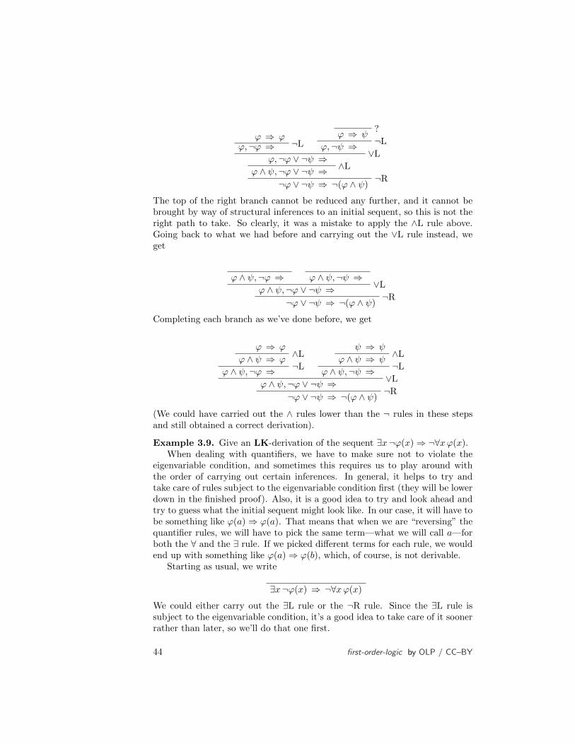
ϕ ⇒ ϕ¬Lϕ,¬ϕ ⇒

?ϕ ⇒ ψ

¬Lϕ,¬ψ ⇒

∨Lϕ,¬ϕ ∨ ¬ψ ⇒

∧Lϕ ∧ ψ,¬ϕ ∨ ¬ψ ⇒

¬R¬ϕ ∨ ¬ψ ⇒ ¬(ϕ ∧ ψ)

The top of the right branch cannot be reduced any further, and it cannot bebrought by way of structural inferences to an initial sequent, so this is not theright path to take. So clearly, it was a mistake to apply the ∧L rule above.Going back to what we had before and carrying out the ∨L rule instead, weget

ϕ ∧ ψ,¬ϕ ⇒ ϕ ∧ ψ,¬ψ ⇒∨L

ϕ ∧ ψ,¬ϕ ∨ ¬ψ ⇒¬R¬ϕ ∨ ¬ψ ⇒ ¬(ϕ ∧ ψ)

Completing each branch as we’ve done before, we get

ϕ ⇒ ϕ∧L

ϕ ∧ ψ ⇒ ϕ¬L

ϕ ∧ ψ,¬ϕ ⇒

ψ ⇒ ψ∧L

ϕ ∧ ψ ⇒ ψ¬L

ϕ ∧ ψ,¬ψ ⇒∨L

ϕ ∧ ψ,¬ϕ ∨ ¬ψ ⇒¬R¬ϕ ∨ ¬ψ ⇒ ¬(ϕ ∧ ψ)

(We could have carried out the ∧ rules lower than the ¬ rules in these stepsand still obtained a correct derivation).

Example 3.9. Give an LK-derivation of the sequent ∃x¬ϕ(x)⇒ ¬∀xϕ(x).When dealing with quantifiers, we have to make sure not to violate the

eigenvariable condition, and sometimes this requires us to play around withthe order of carrying out certain inferences. In general, it helps to try andtake care of rules subject to the eigenvariable condition first (they will be lowerdown in the finished proof). Also, it is a good idea to try and look ahead andtry to guess what the initial sequent might look like. In our case, it will have tobe something like ϕ(a)⇒ ϕ(a). That means that when we are “reversing” thequantifier rules, we will have to pick the same term—what we will call a—forboth the ∀ and the ∃ rule. If we picked different terms for each rule, we wouldend up with something like ϕ(a)⇒ ϕ(b), which, of course, is not derivable.

Starting as usual, we write

∃x¬ϕ(x) ⇒ ¬∀xϕ(x)

We could either carry out the ∃L rule or the ¬R rule. Since the ∃L rule issubject to the eigenvariable condition, it’s a good idea to take care of it soonerrather than later, so we’ll do that one first.





¬ϕ(a) ⇒ ¬∀xϕ(x)∃L∃x¬ϕ(x) ⇒ ¬∀xϕ(x)

Applying the ¬L and ¬R rules and then eliminating the double ¬ signs on bothsides—the reader may do this as an exercise—we get

∀xϕ(x) ⇒ ϕ(a)

¬ϕ(a) ⇒ ¬∀xϕ(x)∃L∃x¬ϕ(x) ⇒ ¬∀xϕ(x)

At this point, our only option is to carry out the ∀L rule. Since this rule is notsubject to the eigenvariable restriction, we’re in the clear. Remember, we wantto try and obtain an initial sequent (of the form ϕ(a) ⇒ ϕ(a)), so we shouldchoose a as our argument for ϕ when we apply the rule.

ϕ(a) ⇒ ϕ(a)∀L∀xϕ(x) ⇒ ϕ(a)

¬ϕ(a) ⇒ ¬∀xϕ(x)∃L∃x¬ϕ(x) ⇒ ¬∀xϕ(x)

It is important, especially when dealing with quantifiers, to double check atthis point that the eigenvariable condition has not been violated. Since theonly rule we applied that is subject to the eigenvariable condition was ∃L, andthe eigenvariable a does not occur in its lower sequent (the end-sequent), thisis a correct derivation.

Problem 3.1. Give derivations of the following sequents:

1. ⇒ ¬(ϕ→ ψ)→ (ϕ ∧ ¬ψ)

2. ∀x (ϕ(x)→ ψ)⇒ (∃y ϕ(y)→ ψ)

3.3 Proof-Theoretic Notions

fol:seq:ptn:sec

explanationJust as we’ve defined a number of important semantic notions (validity,entailment, satisfiabilty), we now define corresponding proof-theoretic notions.These are not defined by appeal to satisfaction of sentences in structures, butby appeal to the derivability or non-derivability of certain sequents. It was animportant discovery, due to Godel, that these notions coincide. That they dois the content of the completeness theorem.





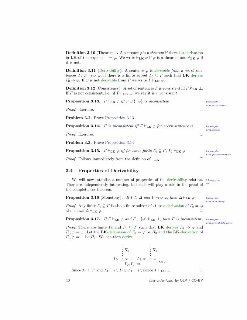
Definition 3.10 (Theorems). A sentence ϕ is a theorem if there is a derivationin LK of the sequent ⇒ ϕ. We write `LK ϕ if ϕ is a theorem and 0LK ϕ ifit is not.

Definition 3.11 (Derivability). A sentence ϕ is derivable from a set of sen-tences Γ , Γ `LK ϕ, if there is a finite subset Γ0 ⊆ Γ such that LK derivesΓ0 ⇒ ϕ. If ϕ is not derivable from Γ we write Γ 0LK ϕ.

Definition 3.12 (Consistency). A set of sentences Γ is consistent iff Γ 0LK ⊥.If Γ is not consistent, i.e., if Γ `LK ⊥, we say it is inconsistent.

Proposition 3.13. fol:seq:ptn:

prop:prov-incons

Γ `LK ϕ iff Γ ∪ ¬ϕ is inconsistent.

Proof. Exercise.



prop:incons

Γ is inconsistent iff Γ `LK ϕ for every sentence ϕ.

Proof. Exercise.



prop:proves-compact

Γ `LK ϕ iff for some finite Γ0 ⊆ Γ , Γ0 `LK ϕ.

Proof. Follows immediately from the definion of `LK.

3.4 Properties of Derivability

fol:seq:prv:sec

We will now establish a number of properties of the derivability relation.They are independently interesting, but each will play a role in the proof ofthe completeness theorem.

Proposition 3.16 (Monotony). fol:seq:prv:

prop:monotony

If Γ ⊆ ∆ and Γ `LK ϕ, then ∆ `LK ϕ.

Proof. Any finite Γ0 ⊆ Γ is also a finite subset of ∆, so a derivation of Γ0 ⇒ ϕalso shows ∆ `LK ϕ.

Proposition 3.17. fol:seq:prv:

prop:provability-contr

If Γ `LK ϕ and Γ ∪ ϕ `LK ⊥, then Γ is inconsistent.

Proof. There are finite Γ0 and Γ1 ⊆ Γ such that LK derives Γ0 ⇒ ϕ andΓ1, ϕ⇒ ⊥. Let the LK-derivation of Γ0 ⇒ ϕ be Π0 and the LK-derivation ofΓ1, ϕ⇒ ⊥ be Π1. We can then derive

Π0

Γ0 ⇒ ϕ

Π1

Γ1, ϕ ⇒ ⊥cut

Γ0, Γ1 ⇒ ⊥Since Γ0 ⊆ Γ and Γ1 ⊆ Γ , Γ0 ∪ Γ1 ⊆ Γ , hence Γ `LK ⊥.





Proposition 3.18.fol:seq:prv:

prop:provability-lnot

If Γ ∪ ϕ `LK ⊥, then Γ `LK ¬ϕ.

Proof. Suppose that Γ ∪ ϕ `LK ⊥. Then there is a finite set Γ0 ⊆ Γ suchthat LK derives Γ0, ϕ ⇒ ⊥. Let Π0 be an LK-derivation of Γ0, ϕ ⇒ ⊥, andconsider

Π0

Γ0, ϕ ⇒ ⊥ ¬RΓ0 ⇒ ⊥,¬ϕ ⊥ ⇒

cutΓ0 ⇒ ¬ϕ


prop:provability-exhaustive

If Γ ∪ ϕ `LK ⊥ and Γ ∪ ¬ϕ `LK ⊥, then Γ `LK ⊥.

Proof. There are finite sets Γ0 ⊆ Γ and Γ1 ⊆ Γ and LK-derivations Π0 andΠ1 of Γ0, ϕ⇒ ⊥ and Γ1,¬ϕ⇒ ⊥, respectively. We can then derive

Π0

Γ0, ϕ ⇒ ⊥ ¬RΓ0 ⇒ ⊥,¬ϕ

Π1

Γ1,¬ϕ ⇒ ⊥cut

Γ0, Γ1 ⇒ ⊥

Since Γ0 ⊆ Γ and Γ1 ⊆ Γ , Γ0 ∪ Γ1 ⊆ Γ . Hence Γ `LK ⊥.


prop:provability-lor-left

If Γ ∪ ϕ `LK ⊥ and Γ ∪ ψ `LK ⊥, then Γ ∪ ϕ ∨ψ `LK ⊥.

Proof. There are finite sets Γ0, Γ1 ⊆ Γ and LK-derivations Π0 and Π1 suchthat

Π0

Γ0, ϕ ⇒ ⊥Γ0, Γ1, ϕ ⇒ ⊥

Π1

Γ1, ψ ⇒ ⊥Γ0, Γ1, ψ ⇒ ⊥ ∨L

Γ0, Γ1, ϕ ∨ ψ ⇒ ⊥(Recall that double inference lines indicate several weakening inferences.)

Since Γ0, Γ1 ⊆ Γ and Γ ∪ ϕ ∨ ψ `LK ⊥.



prop:provability-lor-right

If Γ `LK ϕ or Γ `LK ψ, then Γ `LK ϕ ∨ ψ.

Proof. There is an LK-derivation Π0 and a finite set Γ0 ⊆ Γ such that we canderive





Π0

Γ0 ⇒ ϕ∨R

Γ0 ⇒ ϕ ∨ ψ

Therefore Γ `LK ϕ ∨ ψ. The proof for when Γ `LK ψ is similar.



prop:provability-land-left

If Γ `LK ϕ ∧ ψ then Γ `LK ϕ and Γ `LK ψ.

Proof. If Γ `LK ϕ ∧ ψ, there is a finite set Γ0 ⊆ Γ and an LK-derivation Π0

of Γ0 ⇒ ϕ ∧ ψ. Consider

Π0

Γ0 ⇒ ϕ ∧ ψϕ ⇒ ϕ

∧Lϕ ∧ ψ ⇒ ϕ

cutΓ0 ⇒ ϕ

Hence, Γ `LK ϕ. A similar derivation starting with ψ ⇒ ψ on the right sideshows that Γ `LK ψ.



prop:provability-land-right

If Γ `LK ϕ and Γ `LK ψ, then Γ `LK ϕ ∧ ψ.

Proof. If Γ `LK ϕ as well as Γ `LK ψ, there are finite sets Γ0, Γ1 ⊆ Γ and anLK-derivations Π0 of Γ0 ⇒ ϕ and Π1 of Γ1 ⇒ ϕ. Consider

Π0

Γ0 ⇒ ϕ

Γ0, Γ1 ⇒ ϕ

Π1

Γ1 ⇒ ψ

Γ0, Γ1 ⇒ ψ∧R

Γ0, Γ1 ⇒ ϕ ∧ ψ

Since Γ0 ∪ Γ1 ⊆ Γ , we have Γ `LK ϕ ∧ ψ.



prop:provability-mp

If Γ `LK ϕ and Γ `LK ϕ→ ψ, then Γ `LK ψ.

Proof. Suppose that Γ `LK ϕ and Γ `LK ϕ → ψ. There are finite setsΓ0, Γ1 ⊆ Γ such that there are LK-derivations Π0 of Γ0 ⇒ ϕ and Π1 ofΓ1 ⇒ ϕ→ ψ. Consider:





Π0

Γ1 ⇒ ϕ→ ψ

Π1

Γ0 ⇒ ϕ ψ ⇒ ψ→ L

Γ0, ϕ→ ψ ⇒ ψcut

Γ0, Γ1 ⇒ ψ

Since Γ0 ∪ Γ1 ⊆ Γ , this means that Γ `LK ψ.



prop:provability-lif

If Γ `LK ¬ϕ or Γ `LK ψ, then Γ `LK ϕ→ ψ.

Proof. First suppose Γ `LK ¬ϕ. Then for some finite Γ0 ⊆ Γ there is a LK-derivation of Γ0 ⇒ ¬ϕ. The following derivation shows that Γ `LK ϕ→ ψ:

Π0

Γ0 ⇒ ¬ϕ

ϕ ⇒ ϕ¬R¬ϕ,ϕ ⇒WR

ϕ,¬ϕ ⇒ ψ→ R¬ϕ ⇒ ϕ→ ψcut

Γ0 ⇒ ϕ→ ψ

Now suppose Γ `LK ψ. Then for some finite Γ0 ⊆ Γ there is a LK-derivation of Γ0 ⇒ ψ. The following derivation shows that Γ `LK ϕ→ ψ:

Π0

Γ0 ⇒ ψ

ψ ⇒ ψWL

ϕ,ψ ⇒ ψ→ R

ψ ⇒ ϕ→ ψcut

Γ0 ⇒ ϕ→ ψ


Theorem 3.26.fol:seq:prv:

thm:strong-generalization

If c is a constant not occurring in Γ or ϕ(x) and Γ `LK ϕ(c),then Γ `LK ∀xϕ(x).

Proof. Let Π0 be an LK-derivation of Γ0 ⇒ ϕ(c) for some finite Γ0 ⊆ Γ . Byadding a ∀R inference, we obtain a proof of Γ ⇒ ∀xϕ(x), since c does notoccur in Γ or ϕ(x) and thus the eigenvariable condition is satisfied.

Theorem 3.27.fol:seq:prv:

thm:provability-quantifiers

1. If Γ `LK ϕ(t) then Γ ` ∃xϕ(x).

2. If Γ `LK ∀xϕ(x) then Γ ` ϕ(t).

Proof. 1. Suppose Γ `LK ϕ(t). Then for some finite Γ0 ⊆ Γ , LK derivesΓ0 ⇒ ϕ(t). Add an ∃R inference to get a derivation of Γ0 ⇒ ∃xϕ(x).





2. Suppose Γ `LK ∀xϕ(x). Then there is a finite Γ0 ⊆ Γ and an LK-derivation Π of Γ0 ⇒ ∀xϕ(x). Then

Π

Γ0 ⇒ ∀xϕ(x)

ϕ(t) ⇒ ϕ(t)∀L∀xϕ(x) ⇒ ϕ(t)cut

Γ0 ⇒ ϕ(t)

shows that Γ `LK ϕ(t).

3.5 Soundness

fol:seq:sou:sec

explanation A derivation system, such as the sequent calculus, is sound if it cannotderive things that do not actually hold. Soundness is thus a kind of guaranteedsafety property for derivation systems. Depending on which proof theoreticproperty is in question, we would like to know for instance, that

1. every derivable sentence is valid;

2. if a sentence is derivable from some others, it is also a consequence ofthem;

3. if a set of sentences is inconsistent, it is unsatisfiable.

These are important properties of a derivation system. If any of them donot hold, the derivation system is deficient—it would derive too much. Con-sequently, establishing the soundness of a derivation system is of the utmostimportance.

Because all these proof-theoretic properties are defined via derivability inthe sequent calculus of certain sequents, proving (1)–(3) above requires provingsomething about the semantic properties of derivable sequents. We will firstdefine what it means for a sequent to be valid, and then show that everyderivable sequent is valid. (1)–(3) then follow as corollaries from this result.

Definition 3.28. A structure M satisfies a sequent Γ ⇒ ∆ iff either M 6|= αfor some α ∈ Γ or M |= α for some α ∈ ∆.

A sequent is valid iff every structure M satisfies it.

Theorem 3.29 (Soundness). fol:seq:sou:

sequent-soundness

If LK derives Γ ⇒ ∆, then Γ ⇒ ∆ is valid.

Proof. Let Π be a derivation of Γ ⇒ ∆. We proceed by induction on thenumber of inferences in Π.

If the number of inferences is 0, then Π consists only of an initial sequent.Every initial sequent ϕ⇒ ϕ is obviously valid, since for every M, either M 6|= ϕor M |= ϕ.

If the number of inferences is greater than 0, we distinguish cases accordingto the type of the lowermost inference. By induction hypothesis, we can assume





that the premises of that inference are valid, since the height of the proof ofany premise is smaller than n.

First, we consider the possible inferences with only one premise Γ ′ ⇒ ∆′.

1. The last inference is a weakening. Then Γ ′ ⊆ Γ and ∆ = ∆′ if it’s aweakening on the left, or Γ = Γ ′ and ∆′ ⊆ ∆ if it’s a weaking on theright. In either case, ∆′ ⊆ ∆ and Γ ′ ⊆ Γ . If M 6|= α for some α ∈ Γ ′,then, since Γ ′ ⊆ Γ , α ∈ Γ as well, and so M 6|= α for the same α ∈ Γ .Similarly, if M |= α for some α ∈ ∆′, as α ∈ ∆, M |= α for someα ∈ ∆. Since Γ ′ ⇒ ∆′ is valid, one of these cases obtains for every M.Consequently, Γ ⇒ ∆ is valid.

2. The last inference is ¬L: Then for some ϕ ∈ ∆′, ¬ϕ ∈ Γ . Also, Γ ′ ⊆ Γ ,and ∆′ \ ϕ ⊆ ∆.

If M |= ϕ, then M 6|= ¬ϕ, and since ¬ϕ ∈ Γ , M satisfies Γ ⇒ ∆. SinceΓ ′ ⇒ ∆′ is valid, if M 6|= ϕ, then either M 6|= α for some α ∈ Γ ′ orM |= α for some α ∈ ∆′ different from ϕ. Consequently, M 6|= α for someα ∈ Γ (since Γ ′ ⊆ Γ ) or M |= α for some α ∈ ∆′ different from ϕ (since∆′ \ ϕ ⊆ ∆).

3. The last inference is ¬R: Exercise.

4. The last inference is ∧L: There are two variants: ϕ∧ψ may be inferred onthe left from ϕ or from ψ on the left side of the premise. In the first case,ϕ ∈ Γ ′. Consider a structure M. Since Γ ′ ⇒ ∆′ is valid, (a) M 6|= ϕ,(b) M 6|= α for some α ∈ Γ ′ \ ϕ, or (c) M |= α for some α ∈ ∆′. Incase (a), M 6|= ϕ ∧ ψ. In case (b), there is an α ∈ Γ \ ϕ ∧ ψ such thatM 6|= α, since Γ ′ \ ϕ ⊆ Γ \ ϕ ∧ ψ. In case (c), there is a α ∈ ∆ suchthat M |= α, as ∆ = ∆′. So in each case, M satisfies ϕ ∧ ψ, Γ ⇒ ∆.Since M was arbitrary, Γ ⇒ ∆ is valid. The case where ϕ∧ψ is inferredfrom ψ is handled the same, changing ϕ to ψ.

5. The last inference is ∨R: There are two variants: ϕ ∨ ψ may be inferredon the right from ϕ or from ψ on the right side of the premise. In thefirst case, ϕ ∈ ∆′. Consider a structure M. Since Γ ′ ⇒ ∆′ is valid, (a)M |= ϕ, (b) M 6|= α for some α ∈ Γ ′, or (c) M |= α for some α ∈ ∆′\ϕ.In case (a), M |= ϕ ∨ ψ. In case (b), there is α ∈ Γ such that M 6|= α,as Γ = Γ ′. In case (c), there is an α ∈ ∆ such that M |= α, since∆′ \ ϕ ⊆ ∆. So in each case, M satisfies ϕ ∧ ψ, Γ ⇒ ∆. Since M wasarbitrary, Γ ⇒ ∆ is valid. The case where ϕ ∨ ψ is inferred from ψ ishandled the same, changing ϕ to ψ.

6. The last inference is → R: Then ϕ ∈ Γ ′, ψ ∈ ∆′, Γ ′ \ ϕ ⊆ Γ and∆′ \ ψ ⊆ ∆. Since Γ ′ ⇒ ∆′ is valid, for any structure M, (a) M 6|= ϕ,(b) M |= ψ, (c) M 6|= α for some α ∈ Γ ′ \ ϕ, or M |= α for someα ∈ ∆′ \ ψ. In cases (a) and (b), M |= ϕ → ψ. In case (c), for someα ∈ Γ , M 6|= α. In case (d), for some α ∈ ∆, M |= α. In each case, Msatisfies Γ ⇒ ∆. Since M was arbitrary, Γ ⇒ ∆ is valid.





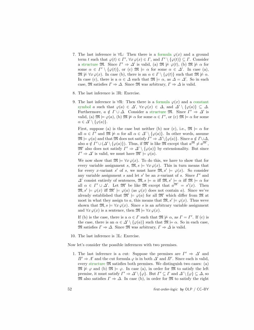
7. The last inference is ∀L: Then there is a formula ϕ(x) and a groundterm t such that ϕ(t) ∈ Γ ′, ∀xϕ(x) ∈ Γ , and Γ ′ \ ϕ(t) ⊆ Γ . Considera structure M. Since Γ ′ ⇒ ∆′ is valid, (a) M 6|= ϕ(t), (b) M 6|= α forsome α ∈ Γ ′ \ ϕ(t), or (c) M |= α for some α ∈ ∆′. In case (a),M 6|= ∀xϕ(x). In case (b), there is an α ∈ Γ \ ϕ(t) such that M 6|= α.In case (c), there is a α ∈ ∆ such that M |= α, as ∆ = ∆′. So in eachcase, M satisfies Γ ⇒ ∆. Since M was arbitrary, Γ ⇒ ∆ is valid.

8. The last inference is ∃R: Exercise.

9. The last inference is ∀R: Then there is a formula ϕ(x) and a constantsymbol a such that ϕ(a) ∈ ∆′, ∀xϕ(x) ∈ ∆, and ∆′ \ ϕ(a) ⊆ ∆.Furthermore, a /∈ Γ ∪ ∆. Consider a structure M. Since Γ ′ ⇒ ∆′ isvalid, (a) M |= ϕ(a), (b) M 6|= α for some α ∈ Γ ′, or (c) M |= α for someα ∈ ∆′ \ ϕ(a).First, suppose (a) is the case but neither (b) nor (c), i.e., M |= α forall α ∈ Γ ′ and M 6|= α for all α ∈ ∆′ \ ϕ(a). In other words, assumeM |= ϕ(a) and that M does not satisfy Γ ′ ⇒ ∆′\ϕ(a). Since a /∈ Γ∪∆,also a /∈ Γ ′ ∪ (∆′ \ ϕ(a)). Thus, if M′ is like M except that aM 6= aM

′,

M′ also does not satisfy Γ ′ ⇒ ∆′ \ ϕ(a) by extensionality. But sinceΓ ′ ⇒ ∆′ is valid, we must have M′ |= ϕ(a).

We now show that M |= ∀xϕ(x). To do this, we have to show that forevery variable assignment s, M, s |= ∀xϕ(x). This in turn means thatfor every x-variant s′ of s, we must have M, s′ |= ϕ(x). So considerany variable assignment s and let s′ be an x-variant of s. Since Γ ′ and∆′ consist entirely of sentences, M, s |= α iff M, s′ |= α iff M |= α forall α ∈ Γ ′ ∪ ∆′. Let M′ be like M except that aM

′= s′(x). Then

M, s′ |= ϕ(x) iff M′ |= ϕ(a) (as ϕ(x) does not contain a). Since we’vealready established that M′ |= ϕ(a) for all M′ which differ from M atmost in what they assign to a, this means that M, s′ |= ϕ(x). Thus weveshown that M, s |= ∀xϕ(x). Since s is an arbitrary variable assignmentand ∀xϕ(x) is a sentence, then M |= ∀xϕ(x).

If (b) is the case, there is a α ∈ Γ such that M 6|= α, as Γ = Γ ′. If (c) isthe case, there is an α ∈ ∆′ \ ϕ(a) such that M |= α. So in each case,M satisfies Γ ⇒ ∆. Since M was arbitrary, Γ ⇒ ∆ is valid.

10. The last inference is ∃L: Exercise.

Now let’s consider the possible inferences with two premises.

1. The last inference is a cut: Suppose the premises are Γ ′ ⇒ ∆′ andΠ ′ ⇒ Λ′ and the cut formula ϕ is in both ∆′ and Π ′. Since each is valid,every structure M satisfies both premises. We distinguish two cases: (a)M 6|= ϕ and (b) M |= ϕ. In case (a), in order for M to satisfy the leftpremise, it must satisfy Γ ′ ⇒ ∆′ \ϕ. But Γ ′ ⊆ Γ and ∆′ \ϕ ⊆ ∆, soM also satisfies Γ ⇒ ∆. In case (b), in order for M to satisfy the right





premise, it must satisfy Π ′ \ ϕ ⇒ Λ′. But Π ′ \ ϕ ⊆ Γ and Λ′ ⊆ ∆,so M also satisfies Γ ⇒ ∆.

2. The last inference is ∧R. The premises are Γ ⇒ ∆′ and Γ ⇒ ∆′′, whereϕ ∈ ∆′ an ψ ∈ ∆′′. By induction hypothesis, both are valid. Consider astructure M. We have two cases: (a) M 6|= ϕ ∧ ψ or (b) M |= ϕ ∧ ψ. Incase (a), either M 6|= ϕ or M 6|= ψ. In the former case, in order for Mto satisfy Γ ⇒ ∆′, it must already satisfy Γ ⇒ ∆′ \ ϕ. In the lattercase, it must satisfy Γ ⇒ ∆′′ \ ψ. But since both ∆′ \ ϕ ⊆ ∆ and∆′′ \ ψ ⊆ ∆, that means M satisfies Γ ⇒ ∆. In case (b), M satisfiesΓ ⇒ ∆ since ϕ ∧ ψ ∈ ∆.

3. The last inference is ∨L: Exercise.

4. The last inference is → L. The premises are Γ ⇒ ∆′ and Γ ′ ⇒ ∆, whereϕ ∈ ∆′ and ψ ∈ Γ ′. By induction hypothesis, both are valid. Consider astructure M. We have two cases: (a) M |= ϕ → ψ or (b) M 6|= ϕ → ψ.In case (a), either M 6|= ϕ or M |= ψ. In the former case, in order for Mto satisfy Γ ⇒ ∆′, it must already satisfy Γ ⇒ ∆′ \ ϕ. In the lattercase, it must satisfy Γ ′ \ ψ ⇒ ∆. But since both ∆′ \ ϕ ⊆ ∆ andΓ ′ \ ψ ⊆ Γ , that means M satisfies Γ ⇒ ∆. In case (b), M satisfiesΓ ⇒ ∆ since ϕ→ ψ ∈ Γ .

Problem 3.10. Complete the proof of Theorem 3.29.

Corollary 3.30.fol:seq:sou:

weak-soundness

If `LK ϕ then ϕ is valid.


entailment-soundness

If Γ `LK ϕ then Γ ϕ.

Proof. If Γ `LK ϕ then for some finite subset Γ0 ⊆ Γ , there is a derivation ofΓ0 ⇒ ϕ. By Theorem 3.29, every structure M either makes some ψ ∈ Γ0 falseor makes ϕ true. Hence, if M |= Γ then also M |= ϕ.


consistency-soundness

If Γ is satisfiable, then it is consistent.

Proof. We prove the contrapositive. Suppose that Γ is not consistent. ThenΓ `LK ⊥, i.e., there is a finite Γ0 ⊆ Γ and a derivation of Γ0 ⇒ ⊥. ByTheorem 3.29, Γ0 ⇒ ⊥ is valid. Since M 6|= ⊥ for every structure M, for M tosatisfy Γ0 ⇒ ⊥ there must be an α ∈ Γ0 so that M 6|= α, and since Γ0 ⊆ Γ , thatα is also in Γ . In other words, no M satisfies Γ , i.e., Γ is not satisfiable.

3.6 Derivations with Identity predicate

fol:seq:ide:sec

Derivations with the identity predicate require additional inference rules.

Initial sequents for =: If t is a closed term, then ⇒ t = t is an initialsequent.





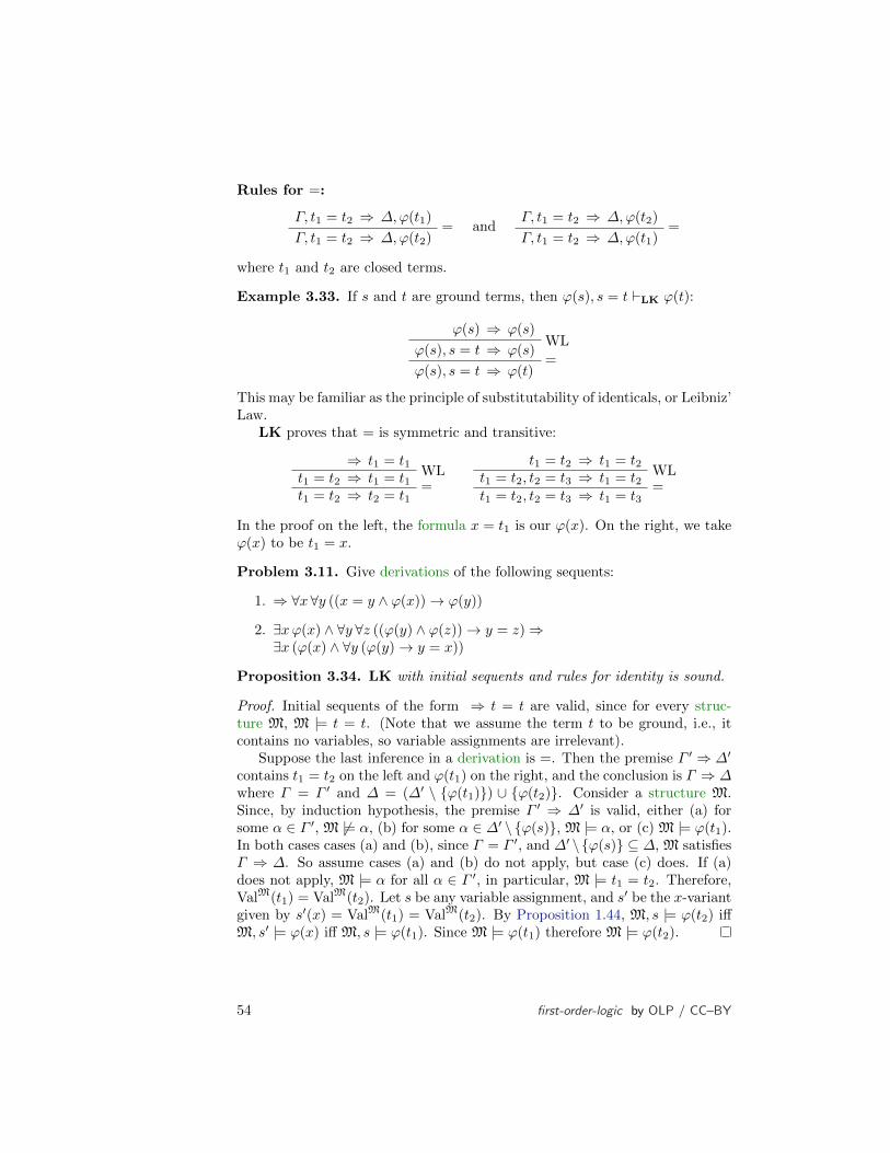
Rules for =:

Γ, t1 = t2 ⇒ ∆,ϕ(t1)=

Γ, t1 = t2 ⇒ ∆,ϕ(t2)and

Γ, t1 = t2 ⇒ ∆,ϕ(t2)=

Γ, t1 = t2 ⇒ ∆,ϕ(t1)

where t1 and t2 are closed terms.

Example 3.33. If s and t are ground terms, then ϕ(s), s = t `LK ϕ(t):

ϕ(s) ⇒ ϕ(s)WL

ϕ(s), s = t ⇒ ϕ(s)=

ϕ(s), s = t ⇒ ϕ(t)

This may be familiar as the principle of substitutability of identicals, or Leibniz’Law.

LK proves that = is symmetric and transitive:

⇒ t1 = t1WLt1 = t2 ⇒ t1 = t1 =

t1 = t2 ⇒ t2 = t1

t1 = t2 ⇒ t1 = t2WLt1 = t2, t2 = t3 ⇒ t1 = t2 =

t1 = t2, t2 = t3 ⇒ t1 = t3

In the proof on the left, the formula x = t1 is our ϕ(x). On the right, we takeϕ(x) to be t1 = x.

Problem 3.11. Give derivations of the following sequents:

1. ⇒ ∀x∀y ((x = y ∧ ϕ(x))→ ϕ(y))

2. ∃xϕ(x) ∧ ∀y ∀z ((ϕ(y) ∧ ϕ(z))→ y = z)⇒∃x (ϕ(x) ∧ ∀y (ϕ(y)→ y = x))

Proposition 3.34. LK with initial sequents and rules for identity is sound.

Proof. Initial sequents of the form ⇒ t = t are valid, since for every struc-ture M, M |= t = t. (Note that we assume the term t to be ground, i.e., itcontains no variables, so variable assignments are irrelevant).

Suppose the last inference in a derivation is =. Then the premise Γ ′ ⇒ ∆′

contains t1 = t2 on the left and ϕ(t1) on the right, and the conclusion is Γ ⇒ ∆where Γ = Γ ′ and ∆ = (∆′ \ ϕ(t1)) ∪ ϕ(t2). Consider a structure M.Since, by induction hypothesis, the premise Γ ′ ⇒ ∆′ is valid, either (a) forsome α ∈ Γ ′, M 6|= α, (b) for some α ∈ ∆′ \ ϕ(s), M |= α, or (c) M |= ϕ(t1).In both cases cases (a) and (b), since Γ = Γ ′, and ∆′ \ϕ(s) ⊆ ∆, M satisfiesΓ ⇒ ∆. So assume cases (a) and (b) do not apply, but case (c) does. If (a)does not apply, M |= α for all α ∈ Γ ′, in particular, M |= t1 = t2. Therefore,ValM(t1) = ValM(t2). Let s be any variable assignment, and s′ be the x-variantgiven by s′(x) = ValM(t1) = ValM(t2). By Proposition 1.44, M, s |= ϕ(t2) iffM, s′ |= ϕ(x) iff M, s |= ϕ(t1). Since M |= ϕ(t1) therefore M |= ϕ(t2).





Chapter 4

Natural Deduction

4.1 Introduction

fol:ntd:int:sec

Logical systems commonly have not just a semantics, but also proof sys-tems. The purpose of proof systems is to provide a purely syntactic method ofestablishing entailment and validity. They are purely syntactic in the sense thata derivation in such a system is a finite syntactic object, usually a sequence (orother finite arrangement) of formulas. Moreover, good proof systems have theproperty that any given sequence or arrangement of formulas can be verifiedmechanically to be a “correct” proof. The simplest (and historically first) proofsystems for first-order logic were axiomatic. A sequence of formulas counts asa derivation in such a system if each individual formula in it is either among afixed set of “axioms” or follows from formulas coming before it in the sequenceby one of a fixed number of “inference rules”—and it can be mechanicallyverified if a formula is an axiom and whether it follows correctly from otherformulas by one of the inference rules. Axiomatic proof systems are easy todescribe—and also easy to handle meta-theoretically—but derivations in themare hard to read and understand, and are also hard to produce.

Other proof systems have been developed with the aim of making it eas-ier to construct derivations or easier to understand derivations once they arecomplete. Examples are truth trees, also known as tableaux proofs, and thesequent calculus. Some proof systems are designed especially with mechaniza-tion in mind, e.g., the resolution method is easy to implement in software (butits derivations are essentially impossible to understand). Most of these otherproof systems represent derivations as trees of formulas rather than sequences.This makes it easier to see which parts of a derivation depend on which otherparts.

The proof system we will study is Gentzen’s natural deduction. Naturaldeduction is intended to mirror actual reasoning (especially the kind of reg-imented reasoning employed by mathematicians). Actual reasoning proceedsby a number of “natural” patterns. For instance proof by cases allows us toestablish a conclusion on the basis of a disjunctive premise, by establishing that

55

the conclusion follows from either of the disjuncts. Indirect proof allows us toestablish a conclusion by showing that its negation leads to a contradiction.Conditional proof establishes a conditional claim “if . . . then . . . ” by showingthat the consequent follows from the antecedent. Natural deduction is a for-malization of some of these natural inferences. Each of the logical connectivesand quantifiers comes with two rules, an introduction and an elimination rule,and they each correspond to one such natural inference pattern. For instance,→ Intro corresponds to conditional proof, and ∨Elim to proof by cases.

One feature that distinguishes natural deduction from other proof systemsis its use of assumptions. In almost every proof system a single formula is at theroot of the tree of formulas—usually the conclusion—and the “leaves” of thetree are formulas from which the conclusion is derived. In natural deduction,some leaf formulas play a role inside the derivation but are “used up” by thetime the derivation reaches the conclusion. This corresponds to the practice,in actual reasoning, of introducing hypotheses which only remain in effect fora short while. For instance, in a proof by cases, we assume the truth of eachof the disjuncts; in conditional proof, we assume the truth of the antecedent;in indirect proof, we assume the truth of the negation of the conclusion. Thisway of introducing hypotheticals and then doing away with them in the serviceof establishing an intermediate step is a hallmark of natural deduction. Theformulas at the leaves of a natural deduction derivation are called assumptions,and some of the rules of inference may “discharge” them. An assumption thatremains undischarged at the end of the derivation is (usually) essential to thetruth of the conclusion, and so a derivation establishes that its undischargedassumptions entail its conclusion.

For any proof system it is crucial to verify that it in fact does what it’ssupposed to: provide a way to verify that a sentence is entailed by some others.This is called soundness; and we will prove it for the natural deduction systemwe use. It is also crucial to verify the converse: that the proof system is strongenough to verify that Γ ϕ whenever this holds, that there is a derivation of ϕfrom Γ whenever Γ ϕ. This is called completeness—but it is much harder toprove.

4.2 Rules and Derivations

fol:ntd:rul:sec

Let L be a first-order language with the usual constant symbols, variables,logical symbols, and auxiliary symbols (parentheses and the comma).

Definition 4.1 (Inference). An inference is an expression of the form

ϕχ or ϕ ψ

χ

where ϕ,ψ, and χ are formulas. ϕ and ψ are called the upper formulas orpremises and χ the lower formulas or conclusion of the inference.

The rules for natural deduction are divided into two main types: proposi-tional rules (quantifier-free) and quantifier rules. The rules come in pairs, an





introduction and an elimination rule for each logical operator. They introduceda logical operator in the conclusion or remove a logical operator from a premiseof the rule. Some of the rules allow an assumption of a certain type to be dis-charged. To indicate which assumption is discharged by which inference, wealso assign labels to both the assumption and the inference. This is indicatedby writing the assumption formula as “[ϕ]n”.

It is customary to consider rules for all logical operators, even for those (ifany) that we consider as defined.

Propositional Rules

Rules for ⊥ ϕ ¬ϕ⊥Intro⊥

⊥ ⊥Elimϕ

Rules for ∧

ϕ ψ∧Intro

ϕ ∧ ψϕ ∧ ψ

∧Elimϕϕ ∧ ψ

∧Elimψ

Rules for ∨

ϕ∨Intro

ϕ ∨ ψψ

∨Introϕ ∨ ψ

ϕ ∨ ψ

[ϕ]n

χ

[ψ]n

χn ∨Elimχ

Rules for ¬[ϕ]n

⊥n ¬Intro¬ϕ

¬¬ϕ¬Elimϕ

Rules for →

[ϕ]n

ψn → Introϕ→ ψ

ϕ ϕ→ ψ→ Elim

ψ

Quantifier Rules

Rules for ∀ϕ(a)

∀Intro∀xϕ(x)

∀xϕ(x)∀Elim

ϕ(t)





where t is a ground term (a term that does not contain any variables), anda is a constant symbol which does not occur in ϕ, or in any assumption whichis undischarged in the derivation ending with the premise ϕ. We call a theeigenvariable of the ∀Intro inference.

Rules for ∃

ϕ(t)∃Intro∃xϕ(x)

∃xϕ(x)

[ϕ(a)]n

χn ∃Elimχ

where t is a ground term, and a is a constant which does not occur in thepremise ∃xϕ(x), in χ, or any assumption which is undischarged in the deriva-tions ending with the two premises χ (other than the assumptions ϕ(a)). Wecall a the eigenvariable of the ∃Elim inference.

The condition that an eigenvariable neither occur in the premises nor inany assumption that is undischarged in the derivations leading to the premisesfor the ∀Intro or ∃Elim inference is called the eigenvariable condition.

explanation We use the term “eigenvariable” even though a in the above rules is aconstant. This has historical reasons.

In ∃Intro and ∀Elim there are no restrictions, and the term t can be any-thing, so we do not have to worry about any conditions. On the other hand,in the ∃Elim and ∀Intro rules, the eigenvariable condition requires that a doesnot occur anywhere else in the formula. Thus, if the upper formula is valid,the truth values of the formulas other than ϕ(a) are independent of a.

explanation Natural deduction systems are meant to closely parallel the informal rea-soning used in mathematical proof (hence it is somewhat “natural”). Naturaldeduction proofs begin with assumptions. Inference rules are then applied. As-sumptions are “discharged” by the ¬Intro,→ Intro, ∨Elim and ∃Elim inferencerules, and the label of the discharged assumption is placed beside the inferencefor clarity.

Definition 4.2 (Initial Formula). An initial formula or assumption is anyformula in the topmost position of any branch.

Definition 4.3 (Derivation). A derivation of a formula ϕ from assumptions Γis a tree of formulas satisfying the following conditions:

1. The topmost formulas of the tree are either in Γ or are discharged by aninference in the tree.

2. Every formula in the tree is an upper formula of an inference whose lowerformula stands directly below that formula in the tree.

We then say that ϕ is the end-formula of the derivation and that ϕ is derivablefrom Γ .





4.3 Examples of Derivations

fol:ntd:pro:sec

Example 4.4. Let’s give a derivation of the formula (ϕ ∧ ψ)→ ϕ.We begin by writing the desired end-formula at the bottom of the derivation.

(ϕ ∧ ψ)→ ϕ

Next, we need to figure out what kind of inference could result in a formulaof this form. The main operator of the end-formula is →, so we’ll try toarrive at the end-formula using the → Intro rule. It is best to write down theassumptions involved and label the inference rules as you progress, so it is easyto see whether all assumptions have been discharged at the end of the proof.

[ϕ ∧ ψ]1

ϕ1 → Intro

(ϕ ∧ ψ)→ ϕ

We now need to fill in the steps from the assumption ϕ ∧ ψ to ϕ. Since weonly have one connective to deal with, ∧, we must use the ∧ elim rule. Thisgives us the following proof:

[ϕ ∧ ψ]1∧Elimϕ

1 → Intro(ϕ ∧ ψ)→ ϕ

We now have a correct derivation of the formula (ϕ ∧ ψ)→ ϕ.

Example 4.5. Now let’s give a derivation of the formula (¬ϕ∨ψ)→ (ϕ→ ψ).We begin by writing the desired end-formula at the bottom of the derivation.

(¬ϕ ∨ ψ)→ (ϕ→ ψ)

To find a logical rule that could give us this end-formula, we look at the logicalconnectives in the end-formula: ¬, ∨, and →. We only care at the momentabout the first occurence of → because it is the main operator of the sentencein the end-sequent, while ¬, ∨ and the second occurence of → are inside thescope of another connective, so we will take care of those later. We thereforestart with the → Intro rule. A correct application must look as follows:

[¬ϕ ∨ ψ]1

ϕ→ ψ1 → Intro

(¬ϕ ∨ ψ)→ (ϕ→ ψ)





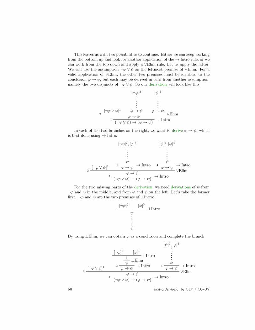
This leaves us with two possibilities to continue. Either we can keep workingfrom the bottom up and look for another application of the→ Intro rule, or wecan work from the top down and apply a ∨Elim rule. Let us apply the latter.We will use the assumption ¬ϕ ∨ ψ as the leftmost premise of ∨Elim. For avalid application of ∨Elim, the other two premises must be identical to theconclusion ϕ→ ψ, but each may be derived in turn from another assumption,namely the two disjuncts of ¬ϕ ∨ ψ. So our derivation will look like this:

[¬ϕ ∨ ψ]1

[¬ϕ]2

ϕ→ ψ

[ψ]2

ϕ→ ψ2 ∨Elim

ϕ→ ψ1 → Intro

(¬ϕ ∨ ψ)→ (ϕ→ ψ)

In each of the two branches on the right, we want to derive ϕ → ψ, whichis best done using → Intro.

[¬ϕ ∨ ψ]1

[¬ϕ]2, [ϕ]3

ψ3 → Introϕ→ ψ

[ψ]2, [ϕ]4


2 ∨Elimϕ→ ψ

1 → Intro(¬ϕ ∨ ψ)→ (ϕ→ ψ)

For the two missing parts of the derivation, we need derivations of ψ from¬ϕ and ϕ in the middle, and from ϕ and ψ on the left. Let’s take the formerfirst. ¬ϕ and ϕ are the two premises of ⊥Intro:

[¬ϕ]2 [ϕ]3⊥Intro⊥

ψ

By using ⊥Elim, we can obtain ψ as a conclusion and complete the branch.

[¬ϕ ∨ ψ]1

[¬ϕ]2 [ϕ]3⊥Intro⊥ ⊥Elim


[ψ]2, [ϕ]4


2 ∨Elimϕ→ ψ

1 → Intro(¬ϕ ∨ ψ)→ (ϕ→ ψ)





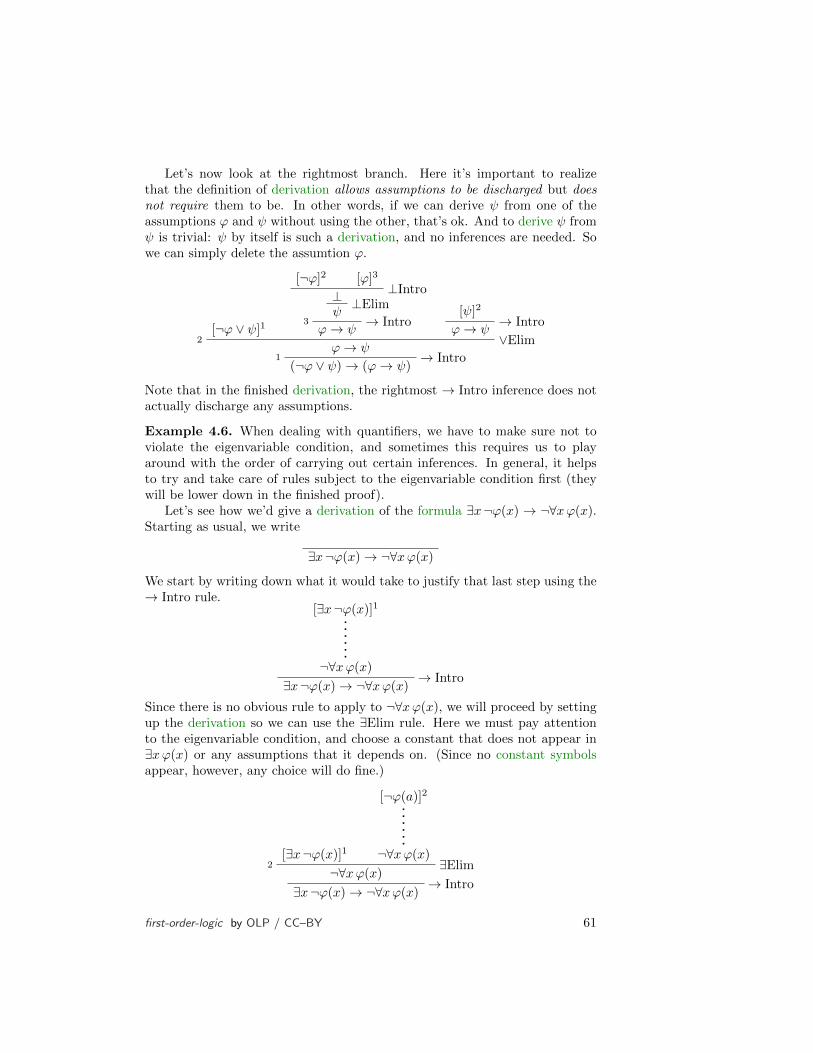
Let’s now look at the rightmost branch. Here it’s important to realizethat the definition of derivation allows assumptions to be discharged but doesnot require them to be. In other words, if we can derive ψ from one of theassumptions ϕ and ψ without using the other, that’s ok. And to derive ψ fromψ is trivial: ψ by itself is such a derivation, and no inferences are needed. Sowe can simply delete the assumtion ϕ.

[¬ϕ ∨ ψ]1

[¬ϕ]2 [ϕ]3⊥Intro⊥ ⊥Elim


[ψ]2→ Intro

ϕ→ ψ2 ∨Elim

ϕ→ ψ1 → Intro

(¬ϕ ∨ ψ)→ (ϕ→ ψ)

Note that in the finished derivation, the rightmost → Intro inference does notactually discharge any assumptions.

Example 4.6. When dealing with quantifiers, we have to make sure not toviolate the eigenvariable condition, and sometimes this requires us to playaround with the order of carrying out certain inferences. In general, it helpsto try and take care of rules subject to the eigenvariable condition first (theywill be lower down in the finished proof).

Let’s see how we’d give a derivation of the formula ∃x¬ϕ(x) → ¬∀xϕ(x).Starting as usual, we write

∃x¬ϕ(x)→ ¬∀xϕ(x)

We start by writing down what it would take to justify that last step using the→ Intro rule.

[∃x¬ϕ(x)]1

¬∀xϕ(x)→ Intro∃x¬ϕ(x)→ ¬∀xϕ(x)

Since there is no obvious rule to apply to ¬∀xϕ(x), we will proceed by settingup the derivation so we can use the ∃Elim rule. Here we must pay attentionto the eigenvariable condition, and choose a constant that does not appear in∃xϕ(x) or any assumptions that it depends on. (Since no constant symbolsappear, however, any choice will do fine.)

[∃x¬ϕ(x)]1

[¬ϕ(a)]2

¬∀xϕ(x)2 ∃Elim¬∀xϕ(x)

→ Intro∃x¬ϕ(x)→ ¬∀xϕ(x)





In order to derive ¬∀xϕ(x), we will attempt to use the ¬Intro rule: this re-quires that we derive a contradiction, possibly using ∀xϕ(x) as an additionalassumption. Of coursem, this contradiction may involve the assumption ¬ϕ(a)which will be discharged by the → Intro inference. We can set it up as follows:

[∃x¬ϕ(x)]1

[¬ϕ(a)]2, [∀xϕ(x)]3

⊥3 ¬Intro¬∀xϕ(x)

2 ∃Elim¬∀xϕ(x)→ Intro∃x¬ϕ(x)→ ¬∀xϕ(x)

It looks like we are close to getting a contradiction. The easiest rule to apply isthe ∀Elim, which has no eigenvariable conditions. Since we can use any termwe want to replace the universally quantified x, it makes the most sense tocontinue using a so we can reach a contradiction.

[∃x¬ϕ(x)]1

[¬ϕ(a)]2[∀xϕ(x)]3

∀Elimϕ(a)

⊥Intro⊥3 ¬Intro¬∀xϕ(x)

2 ∃Elim¬∀xϕ(x)→ Intro∃x¬ϕ(x)→ ¬∀xϕ(x)

It is important, especially when dealing with quantifiers, to double checkat this point that the eigenvariable condition has not been violated. Since theonly rule we applied that is subject to the eigenvariable condition was ∃Elim,and the eigenvariable a does not occur in any assumptions it depends on, thisis a correct derivation.

Problem 4.1. Give derivations of the following formulas:

1. ¬(ϕ→ ψ)→ (ϕ ∧ ¬ψ)

2. ∀x (ϕ(x)→ ψ)→ (∃y ϕ(y)→ ψ)

Example 4.7. Sometimes we may derive a formula from other formulas. Inthese cases, we may have undischarged assumptions. It is important to keeptrack of our assumptions as well as the end goal.

Let’s see how we’d give a derivation of the formula ∃xχ(x, b) from theassumptions ∃x (ϕ(x) ∧ ψ(x)) and ∀x (ψ(x) → χ(x, b). Starting as usual, wewrite the end-formula at the bottom.

∃xχ(x, b)

We have two premises to work with. To use the first, i.e., try to find aderivation of ∃xχ(x, b) from ∃x (ϕ(x) ∧ ψ(x)) we would use the ∃Elim rule.





Since it has an eigenvariable condition, we will apply that rule first. We getthe following:

∃x (ϕ(x) ∧ ψ(x))

[ϕ(a) ∧ ψ(a)]1

∃xχ(x, b)1 ∃Elim∃xχ(x, b)

The two assumptions we are working with share ψ. It may be useful at thispoint to apply ∧Elim to separate out ψ(a).

∃x (ϕ(x) ∧ ψ(x))

[ϕ(a) ∧ ψ(a)]1∧Elim

ψ(a)


The second assumption we have to work with is ∀x (ψ(x)→ χ(x, b). Sincethere is no eigenvariable condition we can instantiate x with the constant sym-bol a using ∀Elim to get ψ(a)→ χ(a, b). We now have ψ(a) and ψ(a)→ χ(a, b).Our next move should be a straightforward application of the → Elim rule.

∃x (ϕ(x) ∧ ψ(x))


ψ(a)

∀x (ψ(x)→ χ(x, b))∀Elim

ψ(a)→ χ(a, b)→ Elim

χ(a, b)


We are so close! One application of ∃Intro and we have reached our goal.

∃x (ϕ(x) ∧ ψ(x))


ψ(a)

∀x (ψ(x)→ χ(x, b))∀Elim

ψ(a)→ χ(a, b)→ Elim

χ(a, b)∃Intro∃xχ(x, b)

1 ∃Elim∃xχ(x, b)

Since we ensured at each step that the eigenvariable conditions were not vio-lated, we can be confident that this is a correct derivation.

Example 4.8. Give a derivation of the formula ¬∀xϕ(x) from the assumptions∀xϕ(x)→ ∃y ψ(y) and ¬∃y ψ(y). Starting as usual, we write the target formulaat the bottom.

¬∀xϕ(x)





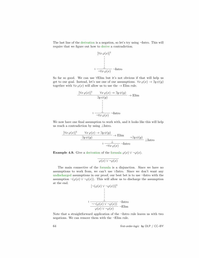
The last line of the derivation is a negation, so let’s try using ¬Intro. This willrequire that we figure out how to derive a contradiction.

[∀xϕ(x)]1


So far so good. We can use ∀Elim but it’s not obvious if that will help usget to our goal. Instead, let’s use one of our assumptions. ∀xϕ(x) → ∃y ψ(y)together with ∀xϕ(x) will allow us to use the → Elim rule.

[∀xϕ(x)]1 ∀xϕ(x)→ ∃y ψ(y)→ Elim∃y ψ(y)


We now have one final assumption to work with, and it looks like this will helpus reach a contradiction by using ⊥Intro.

[∀xϕ(x)]1 ∀xϕ(x)→ ∃y ψ(y)→ Elim∃y ψ(y) ¬∃y ψ(y)

⊥Intro⊥1 ¬Intro¬∀xϕ(x)

Example 4.9. Give a derivation of the formula ϕ(x) ∨ ¬ϕ(x).

ϕ(x) ∨ ¬ϕ(x)

The main connective of the formula is a disjunction. Since we have noassumptions to work from, we can’t use ∨Intro. Since we don’t want anyundischarged assumptions in our proof, our best bet is to use ¬Intro with theassumption ¬(ϕ(x) ∨ ¬ϕ(x)). This will allow us to discharge the assumptionat the end.

[¬(ϕ(x) ∨ ¬ϕ(x))]1

⊥1 ¬Intro¬¬(ϕ(x) ∨ ¬ϕ(x))

¬Elimϕ(x) ∨ ¬ϕ(x)

Note that a straightforward application of the ¬Intro rule leaves us with twonegations. We can remove them with the ¬Elim rule.





We appear to be stuck again, since the assumption we introduced has anegation as the main operator. So let’s try to derive another contradiction!Let’s assume ϕ(x) for another ¬Intro. From there we can derive ϕ(x) ∨ ¬ϕ(x)and get our first contradiction.

[¬(ϕ(x) ∨ ¬ϕ(x))]1[ϕ(x)]2

∨Introϕ(x) ∨ ¬ϕ(x)

⊥Intro⊥2 ¬Intro¬ϕ(x)

⊥1 ¬Intro¬¬(ϕ(x) ∨ ¬ϕ(x))

¬Elimϕ(x) ∨ ¬ϕ(x)

Our second assumption is now discharged. We only need to derive one morecontradiction in order to discharge our first assumption. Now we have some-thing to work with—¬ϕ(x). We can use the same strategy as last time (∨Intro)to derive a contradiction with our first assumption.

[¬(ϕ(x) ∨ ¬ϕ(x))]1[ϕ(x)]2

∨Introϕ(x) ∨ ¬ϕ(x)

⊥Intro⊥2 ¬Intro¬ϕ(x)

∨Introϕ(x) ∨ ¬ϕ(x) [¬(ϕ(x) ∨ ¬ϕ(x))]1

1 ¬Intro¬¬(ϕ(x) ∨ ¬ϕ(x))¬Elim

ϕ(x) ∨ ¬ϕ(x)

And the proof is done!

4.4 Proof-Theoretic Notions

fol:ntd:ptn:sec

explanationJust as we’ve defined a number of important semantic notions (validity,entailment, satisfiabilty), we now define corresponding proof-theoretic notions.These are not defined by appeal to satisfaction of sentences in structures, butby appeal to the derivability or non-derivability of certain formulas. It was animportant discovery, due to Godel, that these notions coincide. That they dois the content of the completeness theorem.

Definition 4.10 (Derivability). A formula ϕ is derivable from a set of formu-las Γ , Γ ` ϕ, if there is a derivation with end-formula ϕ and in which everyassumption is either discharged or is in Γ . If ϕ is not derivable from Γ wewrite Γ 0 ϕ.

Definition 4.11 (Theorems). A formula ϕ is a theorem if there is a derivationof ϕ from the empty set, i.e., a derivation with end-formula ϕ in which all





assumptions are discharged. We write ` ϕ if ϕ is a theorem and 0 ϕ if it isnot.

Definition 4.12 (Consistency). A set of sentences Γ is consistent iff Γ 0 ⊥.If Γ is not consistent, i.e., if Γ ` ⊥, we say it is inconsistent.

Proposition 4.13. fol:ntd:ptn:

prop:prov-incons

Γ ` ϕ iff Γ ∪ ¬ϕ is inconsistent.

Proof. Exercise.



prop:incons

Γ is inconsistent iff Γ ` ϕ for every sentence ϕ.

Proof. Exercise.



prop:proves-compact

Γ ` ϕ iff for some finite Γ0 ⊆ Γ , Γ0 ` ϕ.

Proof. Any derivation of ϕ from Γ can only contain finitely many undischargedassumtions. If all these undischarged assumptions are in Γ , then the set of themis a finite subset of Γ . The other direction is trivial, since a derivation from asubset of Γ is also a derivation from Γ .

4.5 Properties of Derivability

fol:ntd:prv:sec

We will now establish a number of properties of the derivability relation.They are independently interesting, but each will play a role in the proof ofthe completeness theorem.

Proposition 4.16 (Monotony). fol:ntd:prv:

prop:monotony

If Γ ⊆ ∆ and Γ ` ϕ, then ∆ ` ϕ.

Proof. Any derivation of ϕ from Γ is also a derivation of ϕ from ∆.

Proposition 4.17. fol:ntd:prv:

prop:provability-contr

If Γ ` ϕ and Γ ∪ ϕ ` ⊥, then Γ is inconsistent.

Proof. Let the derivation of ϕ from Γ be δ1 and the derivation of ⊥ fromΓ ∪ ϕ be δ2. We can then derive:

δ1

ϕ

[ϕ]1

δ2

⊥1 ¬Intro¬ϕ

¬Elim⊥

In the new derivation, the assumption ϕ is discharged, so it is a derivation fromΓ .





Proposition 4.18.fol:ntd:prv:

prop:provability-lnot

If Γ ∪ ϕ ` ⊥, then Γ ` ¬ϕ.

Proof. Suppose that Γ ∪ϕ ` ⊥. Then there is a derivation of ⊥ from Γ ∪ϕ.Let δ be the derivation of ⊥, and consider

[ϕ]1

δ

⊥1 ¬Intro¬ϕ


prop:provability-exhaustive

If Γ ∪ ϕ ` ⊥ and Γ ∪ ¬ϕ ` ⊥, then Γ ` ⊥.

Proof. There are derivations δ1 and δ2 of ⊥ from Γ∪, ϕ and ⊥ from Γ∪¬ϕ,respectively. We can then derive

[ϕ]1

δ1

⊥1 ¬Intro¬ϕ

[¬ϕ]2

δ2

⊥2 ¬Intro¬¬ϕ

¬Elim⊥

Since the assumptions ϕ and ¬ϕ are discharged, this is a derivation from Γalone. Hence Γ ` ⊥.


prop:provability-lor-left

If Γ ∪ ϕ ` ⊥ and Γ ∪ ψ ` ⊥, then Γ ∪ ϕ ∨ ψ ` ⊥.

Proof. Exercise.



prop:provability-lor-right

If Γ ` ϕ or Γ ` ψ, then Γ ` ϕ ∨ ψ.

Proof. Suppose Γ ` ϕ. There is a derivation δ of ϕ from Γ . We can derive

δ

ϕ∨Intro

ϕ ∨ ψ

Therefore Γ ` ϕ ∨ ψ. The proof for when Γ ` ψ is similar.



prop:provability-land-left

If Γ ` ϕ ∧ ψ then Γ ` ϕ and Γ ` ψ.





Proof. If Γ ` ϕ ∧ ψ, there is a derivation δ of ϕ ∧ ψ from Γ . Consider

δ

ϕ ∧ ψ∧Elimϕ

Hence, Γ ` ϕ. A similar derivation shows that Γ ` ψ.



prop:provability-land-right

If Γ ` ϕ and Γ ` ψ, then Γ ` ϕ ∧ ψ.

Proof. If Γ ` ϕ as well as Γ ` ψ, there are derivations δ1 of ϕ and δ2 of ψ fromΓ . Consider

δ1

ϕ

δ2

ψ∧Intro

ϕ ∧ ψThe undischarged assumptions of the new derivation are all in Γ , so we haveΓ ` ϕ ∧ ψ.



prop:provability-mp

If Γ ` ϕ and Γ ` ϕ→ ψ, then Γ ` ψ.

Proof. Suppose that Γ ` ϕ and Γ ` ϕ→ ψ. There are derivations δ1 of ϕ fromΓ and δ2 of ϕ→ ψ from Γ . Consider:

δ1

ϕ

δ2

ϕ→ ψ→ Elim

ψ

This means that Γ ` ψ.



prop:provability-lif

If Γ ` ¬ϕ or Γ ` ψ, then Γ ` ϕ→ ψ.

Proof. First suppose Γ ` ¬ϕ. Then there is a derivation δ of ¬ϕ from Γ . Thefollowing derivation shows that Γ ` ϕ→ ψ:

[ϕ]1

δ

¬ϕ⊥Intro⊥ ⊥Elim






Now suppose Γ ` ψ. Then there is a derivation δ of ψ from Γ . The followingderivation shows that Γ ` ϕ→ ψ:

[ϕ]1

δ

ψ∧Intro

ϕ ∧ ψ∧Elim



Theorem 4.26.fol:ntd:prv:

thm:strong-generalization

If c is a constant not occurring in Γ or ϕ(x) and Γ ` ϕ(c),then Γ ` ∀xϕ(x).

Proof. Let δ be a derivation of ϕ(c) from Γ . By adding a ∀Intro inference, weobtain a proof of ∀xϕ(x). Since c does not occur in Γ or ϕ(x), the eigenvariablecondition is satisfied.

Theorem 4.27.fol:ntd:prv:

thm:provability-quantifiers

1. If Γ ` ϕ(t) then Γ ` ∃xϕ(x).

2. If Γ ` ∀xϕ(x) then Γ ` ϕ(t).

Proof. 1. Suppose Γ ` ϕ(t). Then there is a derivation δ of ϕ(t) from Γ .The derivation

δ

ϕ(t)∃Intro∃xϕ(x)

shows that Γ ` ∃xϕ(x).

2. Suppose Γ ` ∀xϕ(x). Then there is a derivation δ of ∀xϕ(x) from Γ .The derivation

δ

∀xϕ(x)∀Elim

ϕ(t)

shows that Γ ` ϕ(t).





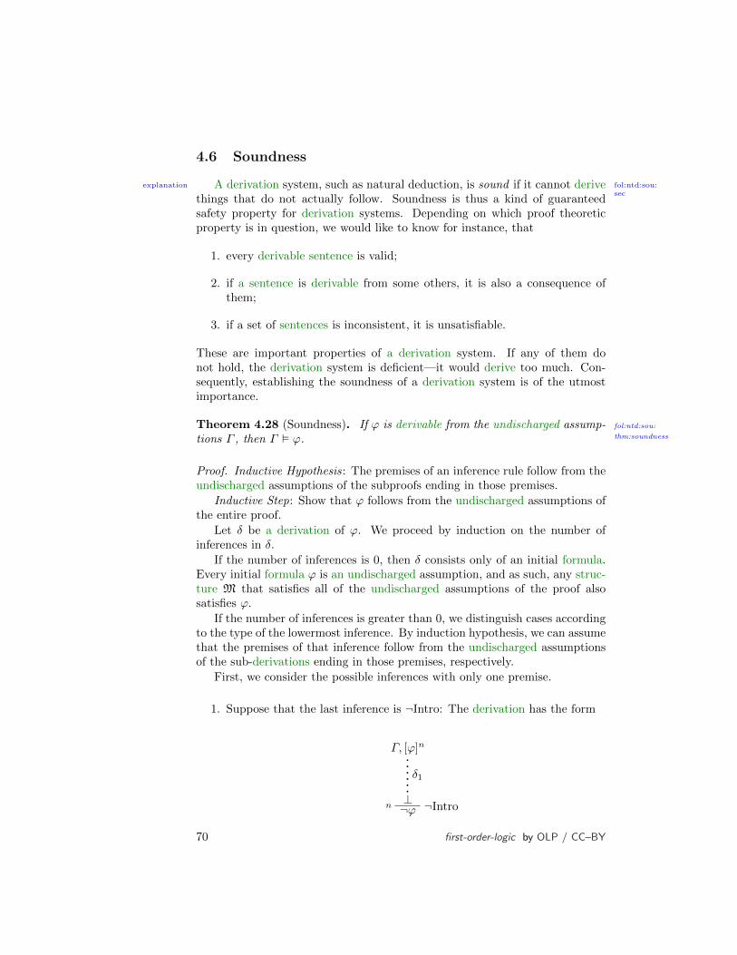
4.6 Soundness

fol:ntd:sou:sec

explanation A derivation system, such as natural deduction, is sound if it cannot derivethings that do not actually follow. Soundness is thus a kind of guaranteedsafety property for derivation systems. Depending on which proof theoreticproperty is in question, we would like to know for instance, that

1. every derivable sentence is valid;

2. if a sentence is derivable from some others, it is also a consequence ofthem;

3. if a set of sentences is inconsistent, it is unsatisfiable.

These are important properties of a derivation system. If any of them donot hold, the derivation system is deficient—it would derive too much. Con-sequently, establishing the soundness of a derivation system is of the utmostimportance.

Theorem 4.28 (Soundness). fol:ntd:sou:

thm:soundness

If ϕ is derivable from the undischarged assump-tions Γ , then Γ ϕ.

Proof. Inductive Hypothesis: The premises of an inference rule follow from theundischarged assumptions of the subproofs ending in those premises.

Inductive Step: Show that ϕ follows from the undischarged assumptions ofthe entire proof.

Let δ be a derivation of ϕ. We proceed by induction on the number ofinferences in δ.

If the number of inferences is 0, then δ consists only of an initial formula.Every initial formula ϕ is an undischarged assumption, and as such, any struc-ture M that satisfies all of the undischarged assumptions of the proof alsosatisfies ϕ.

If the number of inferences is greater than 0, we distinguish cases accordingto the type of the lowermost inference. By induction hypothesis, we can assumethat the premises of that inference follow from the undischarged assumptionsof the sub-derivations ending in those premises, respectively.

First, we consider the possible inferences with only one premise.

1. Suppose that the last inference is ¬Intro: The derivation has the form

Γ, [ϕ]n

δ1

⊥n ¬Intro¬ϕ





By inductive hypothesis, ⊥ follows from the undischarged assumptionsΓ ∪ϕ of δ1. Consider a structure M. We need to show that, if M |= Γ ,then M |= ¬ϕ. Suppose for reductio that M |= Γ , but M 6|= ¬ϕ, i.e.,M |= ϕ. This would mean that M |= Γ ∪ ϕ. This is contrary to ourinductive hypothesis. So, M |= ¬ϕ.

2. The last inference is ¬Elim: Exercise.

3. The last inference is ∧Elim: There are two variants: ϕ or ψ may beinferred from the premise ϕ∧ψ. Consider the first case. The derivation δlooks like this:

Γ

δ1

ϕ ∧ ψ∧Elimϕ

By inductive hypothesis, ϕ ∧ ψ follows from the undischarged assump-tions Γ of δ1. Consider a structure M. We need to show that, if M |= Γ ,then M |= ϕ. Suppose M |= Γ . By our inductive hypothesis (Γ ϕ∨ψ),we know that M |= ϕ ∧ ψ. By definition, M |= ϕ ∧ ψ iff M |= ϕ andM |= ψ. (The case where ψ is inferred from ϕ ∧ ψ is handled similarly.)

4. The last inference is ∨Intro: There are two variants: ϕ ∨ ψ may beinferred from the premise ϕ or the premise ψ. Consider the first case.The derivation has the form

Γ

δ1

ϕ∨Intro

ϕ ∨ ψ

By inductive hypothesis, ϕ follows from the undischarged assumptions Γof δ1. Consider a structure M. We need to show that, if M |= Γ , thenM |= ϕ ∨ ψ. Suppose M |= Γ ; then M |= ϕ since Γ ϕ (the inductivehypothesis). So it must also be the case that M |= ϕ ∨ ψ. (The casewhere ϕ ∨ ψ is inferred from ψ is handled similarly.)

5. The last inference is → Intro: ϕ → ψ is inferred from a subproof withassumption ϕ and conclusion ψ, i.e.,

Γ, [ϕ]n

δ1

ψn → Introϕ→ ψ





By inductive hypothesis, ψ follows from the undischarged assumptionsof δ1, i.e., Γ ∪ ϕ ψ. Consider a structure M. The undischargedassumptions of δ are just Γ , since ϕ is discharged at the last inference.So we need to show that Γ ϕ→ ψ. For reductio, suppose that for somestructure M, M |= Γ but M 6|= ϕ → ψ. So, M |= ϕ and M 6|= ψ. Butby hypothesis, ψ is a consequence of Γ ∪ ϕ, i.e., M |= ψ, which is acontradiction. So, Γ ϕ→ ψ.

6. The last inference is ∀Intro: Then δ has the form

Γ

δ1

ϕ(a)∀Intro∀xA(x)

The premise ϕ(a) is a consequence of the undischarged assumptions Γby induction hypothesis. Consider some structure, M, such that M |= Γ .We need to show that M |= ∀xϕ(x). Since ∀xϕ(x) is a sentence, thismeans we have to show that for every variable assignment s, M, s |= ϕ(x)(Proposition 1.40). Since Γ consists entirely of sentences, M, s |= ψ forall ψ ∈ Γ by Definition 1.34. Let M′ be like M except that aM

′= s(x).

Since a does not occur in Γ , M′ |= Γ by Corollary 1.42. Since Γ A(a),M′ |= A(a). M′, s |= ϕ(x) iff M′ |= ϕ(a) by Proposition 1.44 (recallthat ϕ(a) is just ϕ(x)[a/x]). So, M′, s |= ϕ(x). Since a does not occurin ϕ(x), by Proposition 1.41, M, s |= ϕ(x). But s was an arbitraryvariable assignment, so M |= ∀xϕ(x).

7. The last inference is ∃Intro: Exercise.

8. The last inference is ∀Elim: Exercise.

Now let’s consider the possible inferences with several premises: ∨Elim,∧Intro, → Elim, and ∃Elim.

1. The last inference is ∧Intro. ϕ∧ψ is inferred from the premises ϕ and ψand δ has the form

Γ1

δ1

ϕ

Γ2

δ2

ψ∧Intro

ϕ ∧ ψ

By induction hypothesis, ϕ follows from the undischarged assumptions Γ1

of δ1 and ψ follows from the undischarged assumptions Γ2 of δ2. Theundischarged assumptions of δ are Γ1 ∪ γ2, so we have to show that





Γ1 ∪ Γ2 ϕ ∧ ψ. Consider a structure M with M |= Γ1 ∪ Γ2. SinceM |= Γ1, it must be the case that M |= ϕ as Γ1 ϕ, and since M |= Γ2,M |= ψ since Γ2 ψ. Together, M |= ϕ ∧ ψ.

2. The last inference is ∨Elim: Exercise.

3. The last inference is → Elim. ψ is inferred from the premises ϕ → ψand ϕ. The derivation δ looks like this:

Γ1

δ1

ϕ→ ψ

Γ2

δ2

ϕ→ Elim

ψ

By induction hypothesis, ϕ → ψ follows from the undischarged assump-tions Γ1 of δ1 and ϕ follows from the undischarged assumptions Γ2 of δ2.Consider a structure M. We need to show that, if M |= Γ1 ∪ Γ2, thenM |= ψ. Suppose M |= Γ1 ∪ Γ2. Since Γ1 ϕ → ψ, M |= ϕ → ψ. SinceΓ2 ϕ, we have M |= ϕ. This means that M |= ψ (For if M 6|= ψ, sinceM |= ϕ, we’d have M 6|= ϕ→ ψ, contradicting M |= ϕ→ ψ).

4. The last inference is ∃Elim: Exercise.

Problem 4.10. Complete the proof of Theorem 4.28.

Corollary 4.29.fol:ntd:sou:

cor:weak-soundness

If ` ϕ, then ϕ is valid.

Corollary 4.30.fol:ntd:sou:

cor:consistency-soundness

If Γ is satisfiable, then it is consistent.

Proof. We prove the contrapositive. Suppose that Γ is not consistent. ThenΓ ` ⊥, i.e., there is a derivation of ⊥ from undischarged assumptions in Γ . ByTheorem 4.28, any structure M that satisfies Γ must satisfy ⊥. Since M 6|= ⊥for every structure M, no M can satisfy Γ , i.e., Γ is not satisfiable.

4.7 Derivations with Identity predicate

fol:ntd:ide:sec

Derivations with the identity predicate require additional inference rules.

Rules for =:

= Introt = t

t1 = t2 ϕ(t1)= Elim

ϕ(t2)and

t1 = t2 ϕ(t2)= Elim

ϕ(t1)

where t1 and t2 are closed terms. The = Intro rule allows us to derive anyidentity statement of the form t = t outright, from no assumptions.





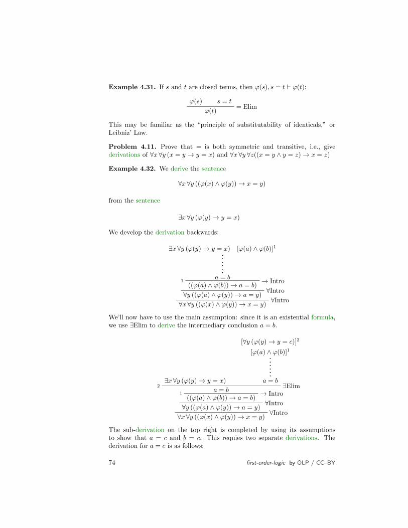
Example 4.31. If s and t are closed terms, then ϕ(s), s = t ` ϕ(t):

ϕ(s) s = t= Elim

ϕ(t)

This may be familiar as the “principle of substitutability of identicals,” orLeibniz’ Law.

Problem 4.11. Prove that = is both symmetric and transitive, i.e., givederivations of ∀x∀y (x = y → y = x) and ∀x ∀y ∀z((x = y ∧ y = z)→ x = z)

Example 4.32. We derive the sentence

∀x∀y ((ϕ(x) ∧ ϕ(y))→ x = y)

from the sentence

∃x∀y (ϕ(y)→ y = x)

We develop the derivation backwards:

∃x∀y (ϕ(y)→ y = x) [ϕ(a) ∧ ϕ(b)]1

a = b1 → Intro

((ϕ(a) ∧ ϕ(b))→ a = b)∀Intro∀y ((ϕ(a) ∧ ϕ(y))→ a = y)∀Intro∀x∀y ((ϕ(x) ∧ ϕ(y))→ x = y)

We’ll now have to use the main assumption: since it is an existential formula,we use ∃Elim to derive the intermediary conclusion a = b.

∃x ∀y (ϕ(y)→ y = x)

[∀y (ϕ(y)→ y = c)]2

[ϕ(a) ∧ ϕ(b)]1

a = b2 ∃Elim

a = b1 → Intro

((ϕ(a) ∧ ϕ(b))→ a = b)∀Intro∀y ((ϕ(a) ∧ ϕ(y))→ a = y)∀Intro∀x ∀y ((ϕ(x) ∧ ϕ(y))→ x = y)

The sub-derivation on the top right is completed by using its assumptionsto show that a = c and b = c. This requies two separate derivations. Thederivation for a = c is as follows:





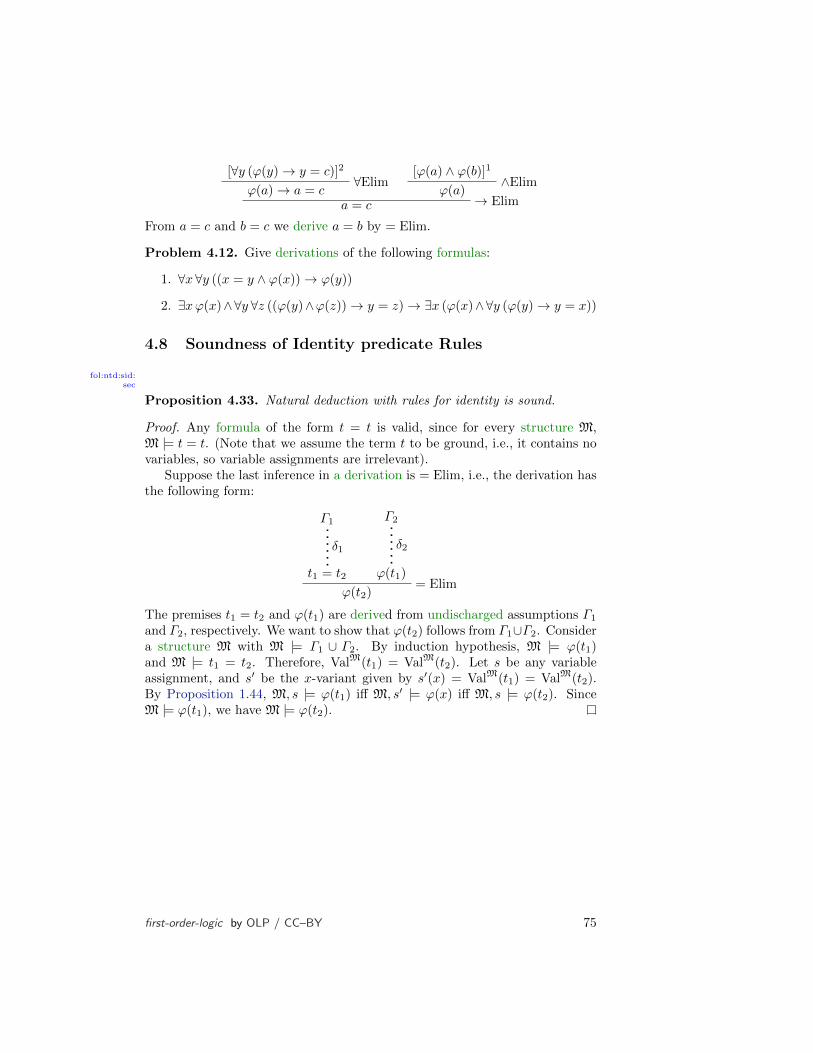
[∀y (ϕ(y)→ y = c)]2∀Elim

ϕ(a)→ a = c

[ϕ(a) ∧ ϕ(b)]1∧Elim

ϕ(a)→ Elima = c

From a = c and b = c we derive a = b by = Elim.

Problem 4.12. Give derivations of the following formulas:

1. ∀x ∀y ((x = y ∧ ϕ(x))→ ϕ(y))

2. ∃xϕ(x)∧∀y ∀z ((ϕ(y)∧ϕ(z))→ y = z)→ ∃x (ϕ(x)∧∀y (ϕ(y)→ y = x))

4.8 Soundness of Identity predicate Rules

fol:ntd:sid:sec

Proposition 4.33. Natural deduction with rules for identity is sound.

Proof. Any formula of the form t = t is valid, since for every structure M,M |= t = t. (Note that we assume the term t to be ground, i.e., it contains novariables, so variable assignments are irrelevant).

Suppose the last inference in a derivation is = Elim, i.e., the derivation hasthe following form:

Γ1

δ1

t1 = t2

Γ2

δ2

ϕ(t1)= Elim

ϕ(t2)

The premises t1 = t2 and ϕ(t1) are derived from undischarged assumptions Γ1

and Γ2, respectively. We want to show that ϕ(t2) follows from Γ1∪Γ2. Considera structure M with M |= Γ1 ∪ Γ2. By induction hypothesis, M |= ϕ(t1)and M |= t1 = t2. Therefore, ValM(t1) = ValM(t2). Let s be any variableassignment, and s′ be the x-variant given by s′(x) = ValM(t1) = ValM(t2).By Proposition 1.44, M, s |= ϕ(t1) iff M, s′ |= ϕ(x) iff M, s |= ϕ(t2). SinceM |= ϕ(t1), we have M |= ϕ(t2).





Chapter 5

The Completeness Theorem

5.1 Introduction

fol:com:int:sec

The completeness theorem is one of the most fundamental results aboutlogic. It comes in two formulations, the equivalence of which we’ll prove. In itsfirst formulation it says something fundamental about the relationship betweensemantic consequence and our proof system: if a sentence ϕ follows from somesentences Γ , then there is also a derivation that establishes Γ ` ϕ. Thus, theproof system is as strong as it can possibly be without proving things thatdon’t actually follow. In its second formulation, it can be stated as a modelexistence result: every consistent set of sentences is satisfiable.

These aren’t the only reasons the completeness theorem—or rather, itsproof—is important. It has a number of important consequences, some ofwhich we’ll discuss separately. For instance, since any derivation that showsΓ ` ϕ is finite and so can only use finitely many of the sentences in Γ , it followsby the completeness theorem that if ϕ is a consequence of Γ , it is already aconsequence of a finite subset of Γ . This is called compactness. Equivalently,if every finite subset of Γ is consistent, then Γ itself must be consistent. Italso follows from the proof of the completeness theorem that any satisfiableset of sentences has a finite or denumerable model. This result is called theLowenheim-Skolem theorem.

5.2 Outline of the Proof

fol:com:out:sec

The proof of the completeness theorem is a bit complex, and upon firstreading it, it is easy to get lost. So let us outline the proof. The first step is ashift of perspective, that allows us to see a route to a proof. When completenessis thought of as “whenever Γ ϕ then Γ ` ϕ,” it may be hard to even come upwith an idea: for to show that Γ ` ϕ we have to find a derivation, and it doesnot look like the hypothesis that Γ ϕ helps us for this in any way. For someproof systems it is possible to directly construct a derivation, but we will takea slightly different tack. The shift in perspective required is this: completeness

77

can also be formulated as: “if Γ is consistent, it has a model.” Perhaps we canuse the information in Γ together with the hypothesis that it is consistent toconstruct a model. After all, we know what kind of model we are looking for:one that is as Γ describes it!

If Γ contains only atomic sentences, it is easy to construct a model forit: for atomic sentences are all of the form P (a1, . . . , an) where the ai areconstant symbols. So all we have to do is come up with a domain |M| andan interpretation for P so that M |= P (a1, . . . , an). But nothing’s easier thanthat: put |M| = N, cMi = i, and for every P (a1, . . . , an) ∈ Γ , put the tuple〈k1, . . . , kn〉 into PM, where ki is the index of the constant symbol ai (i.e.,ai ≡ cki).

Now suppose Γ contains some sentence ¬ψ, with ψ atomic. We might worrythat the construction of M interferes with the possibility of making ¬ψ true.But here’s where the consistency of Γ comes in: if ¬ψ ∈ Γ , then ψ /∈ Γ , or elseΓ would be inconsistent. And if ψ /∈ Γ , then according to our constructionof M, M 6|= ψ, so M |= ¬ψ. So far so good.

Now what if Γ contains complex, non-atomic formulas? Say, it containsϕ∧ψ. Then we should proceed as if both ϕ and ψ were in Γ . And if ϕ∨ψ ∈ Γ ,then we will have to make at least one of them true, i.e., proceed as if one ofthem was in Γ .

This suggests the following idea: we add additional sentences to Γ so as to(a) keep the resulting set consistent and (b) make sure that for every possibleatomic sentence ϕ, either ϕ is in the resulting set, or ¬ϕ, and (c) such that,whenever ϕ∧ψ is in the set, so are both ϕ and ψ, if ϕ∨ψ is in the set, at leastone of ϕ or ψ is also, etc. We keep doing this (potentially forever). Call theset of all sentences so added Γ ∗. Then our construction above would provideus with a structure for which we could prove, by induction, that all sentencesin Γ ∗ are true in M, and hence also all sentence in Γ since Γ ⊆ Γ ∗.

There is one wrinkle in this plan: if ∃xϕ(x) ∈ Γ we would hope to be ableto pick some constant symbol c and add ϕ(c) in this process. But how do weknow we can always do that? Perhaps we only have a few constant symbolsin our language, and for each one of them we have ¬ψ(c) ∈ Γ . We can’t alsoadd ψ(c), since this would make the set inconsistent, and we wouldn’t knowwhether M has to make ψ(c) or ¬ψ(c) true. Moreover, it might happen thatΓ contains only sentences in a language that has no constant symbols at all(e.g., the language of set theory).

The solution to this problem is to simply add infinitely many constants atthe beginning, plus sentences that connect them with the quantifiers in the rightway. (Of course, we have to verify that this cannot introduce an inconsistency.)

Our original construction works well if we only have constant symbols in theatomic sentences. But the language might also contain function symbols. Inthat case, it might be tricky to find the right functions on N to assign to thesefunction symbols to make everything work. So here’s another trick: instead ofusing i to interpret ci, just take the set of constant symbols itself as the domain.Then M can assign every constant symbol to itself: cMi = ci. But why not goall the way: let |M| be all terms of the language! If we do this, there is an





obvious assignment of functions (that take terms as arguments and have termsas values) to function symbols: we assign to the function symbol f ni the functionwhich, given n terms t1, . . . , tn as input, produces the term f ni (t1, . . . , tn) asvalue.

The last piece of the puzzle is what to do with =. The predicate symbol =has a fixed interpretation: M |= t = t′ iff ValM(t) = ValM(t′). Now if we setthings up so that the value of a term t is t itself, then this structure will makeno sentence of the form t = t′ true unless t and t′ are one and the same term.And of course this is a problem, since basically every interesting theory in alanguage with function symbols will have as theorems sentences t = t′ where tand t′ are not the same term (e.g., in theories of arithmetic: (+ ) = ). Tosolve this problem, we change the domain of M: instead of using terms as theobjects in |M|, we use sets of terms, and each set is so that it contains all thoseterms which the sentences in Γ require to be equal. So, e.g., if Γ is a theory ofarithmetic, one of these sets will contain: , (+ ), (× ), etc. This will bethe set we assign to , and it will turn out that this set is also the value of allthe terms in it, e.g., also of ( + ). Therefore, the sentence ( + ) = willbe true in this revised structure.

5.3 Maximally Consistent Sets of Sentences

fol:com:mcs:sec

Definition 5.1 (Maximally consistent set).fol:com:mcs:mcs

A set Γ of sentences is maximallyconsistent iff

1. Γ is consistent, and

2. if Γ ( Γ ′, then Γ ′ is inconsistent.

explanationAn alternate definition equivalent to the above is: a set Γ of sentences ismaximally consistent iff

1. Γ is consistent, and

2. If Γ ∪ ϕ is consistent, then ϕ ∈ Γ .

In other words, one cannot add sentences not already in Γ to a maximallyconsistent set Γ without making the resulting larger set inconsistent.

explanationMaximally consistent sets are important in the completeness proof sincewe can guarantee that every consistent set of sentences Γ is contained in amaximally consistent set Γ ∗, and a maximally consistent set contains, for eachsentence ϕ, either ϕ or its negation ¬ϕ. This is true in particular for atomicsentences, so from a maximally consistent set in a language suitably expandedby constant symbols, we can construct a structure where the interpretation ofpredicate symbols is defined according to which atomic sentences are in Γ ∗.This structure can then be shown to make all sentences in Γ ∗ (and hence alsoin Γ ) true. The proof of this latter fact requires that ¬ϕ ∈ Γ ∗ iff ϕ /∈ Γ ∗,(ϕ ∨ ψ) ∈ Γ ∗ iff ϕ ∈ Γ ∗ or ψ ∈ Γ ∗, etc.





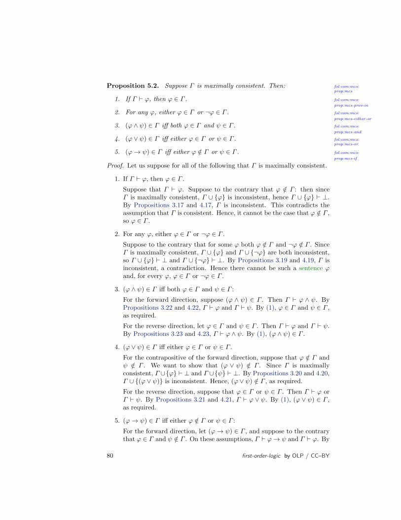
Proposition 5.2. fol:com:mcs:prop:mcs

Suppose Γ is maximally consistent. Then:

1. fol:com:mcs:

prop:mcs-prov-in

If Γ ` ϕ, then ϕ ∈ Γ .

2. fol:com:mcs:

prop:mcs-either-or

For any ϕ, either ϕ ∈ Γ or ¬ϕ ∈ Γ .

3. fol:com:mcs:

prop:mcs-and

(ϕ ∧ ψ) ∈ Γ iff both ϕ ∈ Γ and ψ ∈ Γ .

4. fol:com:mcs:prop:mcs-or

(ϕ ∨ ψ) ∈ Γ iff either ϕ ∈ Γ or ψ ∈ Γ .

5. fol:com:mcs:

prop:mcs-if

(ϕ→ ψ) ∈ Γ iff either ϕ /∈ Γ or ψ ∈ Γ .

Proof. Let us suppose for all of the following that Γ is maximally consistent.

1. If Γ ` ϕ, then ϕ ∈ Γ .

Suppose that Γ ` ϕ. Suppose to the contrary that ϕ /∈ Γ : then sinceΓ is maximally consistent, Γ ∪ ϕ is inconsistent, hence Γ ∪ ϕ ` ⊥.By Propositions 3.17 and 4.17, Γ is inconsistent. This contradicts theassumption that Γ is consistent. Hence, it cannot be the case that ϕ /∈ Γ ,so ϕ ∈ Γ .

2. For any ϕ, either ϕ ∈ Γ or ¬ϕ ∈ Γ .

Suppose to the contrary that for some ϕ both ϕ /∈ Γ and ¬ϕ /∈ Γ . SinceΓ is maximally consistent, Γ ∪ ϕ and Γ ∪ ¬ϕ are both inconsistent,so Γ ∪ ϕ ` ⊥ and Γ ∪ ¬ϕ ` ⊥. By Propositions 3.19 and 4.19, Γ isinconsistent, a contradiction. Hence there cannot be such a sentence ϕand, for every ϕ, ϕ ∈ Γ or ¬ϕ ∈ Γ .

3. (ϕ ∧ ψ) ∈ Γ iff both ϕ ∈ Γ and ψ ∈ Γ :

For the forward direction, suppose (ϕ ∧ ψ) ∈ Γ . Then Γ ` ϕ ∧ ψ. ByPropositions 3.22 and 4.22, Γ ` ϕ and Γ ` ψ. By (1), ϕ ∈ Γ and ψ ∈ Γ ,as required.

For the reverse direction, let ϕ ∈ Γ and ψ ∈ Γ . Then Γ ` ϕ and Γ ` ψ.By Propositions 3.23 and 4.23, Γ ` ϕ ∧ ψ. By (1), (ϕ ∧ ψ) ∈ Γ .

4. (ϕ ∨ ψ) ∈ Γ iff either ϕ ∈ Γ or ψ ∈ Γ .

For the contrapositive of the forward direction, suppose that ϕ /∈ Γ andψ /∈ Γ . We want to show that (ϕ ∨ ψ) /∈ Γ . Since Γ is maximallyconsistent, Γ ∪ϕ ` ⊥ and Γ ∪ψ ` ⊥. By Propositions 3.20 and 4.20,Γ ∪ (ϕ ∨ ψ) is inconsistent. Hence, (ϕ ∨ ψ) /∈ Γ , as required.

For the reverse direction, suppose that ϕ ∈ Γ or ψ ∈ Γ . Then Γ ` ϕ orΓ ` ψ. By Propositions 3.21 and 4.21, Γ ` ϕ ∨ ψ. By (1), (ϕ ∨ ψ) ∈ Γ ,as required.

5. (ϕ→ ψ) ∈ Γ iff either ϕ /∈ Γ or ψ ∈ Γ :

For the forward direction, let (ϕ→ ψ) ∈ Γ , and suppose to the contrarythat ϕ ∈ Γ and ψ /∈ Γ . On these assumptions, Γ ` ϕ→ ψ and Γ ` ϕ. By





Propositions 3.24 and 4.24, Γ ` ψ. But then by (1), ψ ∈ Γ , contradictingthe assumption that ψ /∈ Γ .

For the reverse direction, first consider the case where ϕ /∈ Γ . By (2),¬ϕ ∈ Γ and hence Γ ` ¬ϕ. By Propositions 3.25 and 4.25, Γ ` ϕ → ψ.Again by (1), we get that (ϕ→ ψ) ∈ Γ , as required.

Now consider the case where ψ ∈ Γ . Then Γ ` ψ and by Propositions 3.25and 4.25, Γ ` ϕ→ ψ. By (1), (ϕ→ ψ) ∈ Γ .


5.4 Henkin Expansion

fol:com:hen:sec

explanationPart of the challenge in proving the completeness theorem is that the modelwe construct from a maximally consistent set Γ must make all the quantifiedformulas in Γ true. In order to guarantee this, we use a trick due to LeonHenkin. In essence, the trick consists in expanding the language by infinitelymany constants and adding, for each formula with one free variable ϕ(x) aformula of the form ∃xϕ→ ϕ(c), where c is one of the new constant symbols.When we construct the structure satisfying Γ , this will guarantee that eachtrue existential sentence has a witness among the new constants.

Lemma 5.3.fol:com:hen:

defn:lang-exp

If Γ is consistent in L and L′ is obtained from L by addinga denumerable set of new constant symbols d1, d2, . . . , then Γ is consistentin L′.

Definition 5.4 (Saturated set). A set Γ of formulas of a language L is sat-urated if and only if for each formula ϕ ∈ Frm(L) and variable x there is aconstant symbol c such that ∃xϕ→ ϕ(c) ∈ Γ .

The following definition will be used in the proof of the next theorem.

Definition 5.5. Let L′ be as in Lemma 5.3. Fix an enumeration 〈ϕ1, x1〉,〈ϕ2, x2〉, . . . of all formula-variable pairs of L′. We define the sentences θnby recursion on n. Assuming that θ1, . . . , θn have already been defined, letcn+1 be the first new constant symbol among the di that does not occur in θ1,. . . , θn, and let θn+1 be the formula ∃xn+1 ϕn+1(xn+1) → ϕn+1(cn+1). Thisincludes the case where n = 0 and the list of previous θi’s is empty, i.e., θ1 is∃x1 ϕ1 → ϕ1(c1).

Theorem 5.6.fol:com:hen:

thm:henkin

Every consistent set Γ can be extended to a saturated consis-tent set Γ ′.

Proof. Given a consistent set of sentences Γ in a language L, expand the lan-guage by adding a denumerable set of new constant symbols to form L′. By theprevious Lemma, Γ is still consistent in the richer language. Further, let θi be





as in the previous definition: then Γ ∪θ1, θ2, . . . is saturated by construction.Let

Γ0 = Γ

Γn+1 = Γn ∪ θn+1

i.e., Γn = Γ ∪ θ1, . . . , θn, and let Γ ′ =⋃n Γn. To show that Γ ′ is consistent

it suffices to show, by induction on n, that each set Γn is consistent.The induction basis is simply the claim that Γ0 = Γ is consistent, which is

the hypothesis of the theorem. For the induction step, suppose that Γn−1 isconsistent but Γn = Γn−1∪θn is inconsistent. Recall that θn is ∃xn ϕn(xn)→ϕn(cn). where ϕ(x) is a formula of L′ with only the variable xn free and notcontaining any constant symbols ci where i ≥ n.

If Γn−1 ∪ θn is inconsistent, then Γn−1 ` ¬θn, and hence both of thefollowing hold:

Γn−1 ` ∃xn ϕn(xn) Γn−1 ` ¬ϕn(cn)

Here cn does not occur in Γn−1 or ϕn(xn) (remember, it was added onlywith θn). By Theorems 3.26 and 4.26, from Γ ` ¬ϕn(cn), we obtain Γ `∀xn ¬ϕn(xn). Thus we have that both Γn−1 ` ∃xn ϕn and Γn−1 ` ∀xn ¬ϕn(xn),so Γ itself is inconsistent. (Note that ∀xn ¬ϕn(xn) ` ¬∃xn ϕn(xn).) Contra-diction: Γn−1 was supposed to be consistent. Hence Γn∪θn is consistent.

5.5 Lindenbaum’s Lemma

fol:com:lin:sec

We now prove a lemma that shows that any consistent set of sentences iscontained in some set of sentences which is not just consistent, but maximallyso, and moreover, is saturated. The proof works by first extending the set to asaturated set, and then adding one sentence at a time, guaranteeing at each stepthat the set remains consistent. The union of all stages in that constructionthen contains, for each sentence ϕ, either it or its negation ¬ϕ, is saturated,and is also consistent.

Lemma 5.7 (Lindenbaum’s Lemma). fol:com:lin:

lem:lindenbaum

Every consistent set Γ can be extendedto a maximally consistent saturated set Γ ∗.

Proof. Let Γ be consistent, and let Γ ′ be as in the proof of Theorem 5.6: weproved there that Γ ′ is a consistent saturated set in the richer language L′ (withthe denumerable set of new constants). Let ϕ0, ϕ1, . . . be an enumeration ofall the formulas of L′. Define Γ0 = Γ ′, and

Γn+1 =

Γn ∪ ϕn if Γn ∪ ϕn is consistent;

Γn ∪ ¬ϕn otherwise.

Let Γ ∗ =⋃n≥0 Γn. Since Γ ′ ⊆ Γ ∗, for each formula ϕ, Γ ∗ contains a

formula of the form ∃xϕ→ ϕ(c) and thus is saturated.





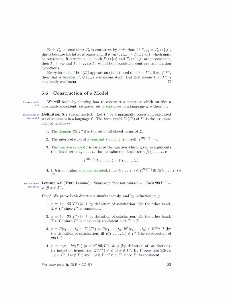
Each Γn is consistent: Γ0 is consistent by definition. If Γn+1 = Γn ∪ ϕ,this is because the latter is consistent. If it isn’t, Γn+1 = Γn∪¬ϕ, which mustbe consistent. If it weren’t, i.e., both Γn ∪ϕ and Γn ∪¬ϕ are inconsistent,then Γn ` ¬ϕ and Γn ` ϕ, so Γn would be inconsistent contrary to inductionhypothesis.

Every formula of Frm(L′) appears on the list used to define Γ ∗. If ϕn /∈ Γ ∗,then that is because Γn ∪ ϕn was inconsistent. But that means that Γ ∗ ismaximally consistent.

5.6 Construction of a Model

fol:com:mod:sec

We will begin by showing how to construct a structure which satisfies amaximally consistent, saturated set of sentences in a language L without =.

Definition 5.8 (Term model).fol:com:mod:

termmodel

Let Γ ∗ be a maximally consistent, saturatedset of sentences in a language L. The term model M(Γ ∗) of Γ ∗ is the structuredefined as follows:

1. The domain |M(Γ ∗)| is the set of all closed terms of L.

2. The interpretation of a constant symbol c is c itself: cM(Γ∗) = c.

3. The function symbol f is assigned the function which, given as argumentsthe closed terms t1, . . . , tn, has as value the closed term f(t1, . . . , tn):

fM(Γ∗)(t1, . . . , tn) = f(t1, . . . , tn)

4. IfR is an n-place predicate symbol, then 〈t1, . . . , tn〉 ∈ RM(Γ∗) iffR(t1, . . . , tn) ∈Γ ∗.

Lemma 5.9 (Truth Lemma).fol:com:mod:

lem:truth

Suppose ϕ does not contain =. Then M(Γ ∗) |=ϕ iff ϕ ∈ Γ ∗.

Proof. We prove both directions simultaneously, and by induction on ϕ.

1. ϕ ≡ ⊥: M(Γ ∗) 6|= ⊥ by definition of satisfaction. On the other hand,⊥ /∈ Γ ∗ since Γ ∗ is consistent.

2. ϕ ≡ >: M(Γ ∗) |= > by definition of satisfaction. On the other hand,> ∈ Γ ∗ since Γ ∗ is maximally consistent and Γ ∗ ` >.

3. ϕ ≡ R(t1, . . . , tn): M(Γ ∗) |= R(t1, . . . , tn) iff 〈t1, . . . , tn〉 ∈ RM(Γ∗) (bythe definition of satisfaction) iff R(t1, . . . , tn) ∈ Γ ∗ (the construction ofM(Γ ∗).

4. ϕ ≡ ¬ψ: M(Γ ∗) |= ϕ iff M(Γ ∗) 6|= ψ (by definition of satisfaction).By induction hypothesis, M(Γ ∗) 6|= ψ iff ψ /∈ Γ ∗. By Proposition 5.2(2),¬ψ ∈ Γ ∗ if ψ /∈ Γ ∗; and ¬ψ /∈ Γ ∗ if ψ ∈ Γ ∗ since Γ ∗ is consistent.





5. ϕ ≡ ψ∧χ: M(Γ ∗) |= ϕ iff we have both M(Γ ∗) |= ψ and M(Γ ∗) |= χ (bydefinition of satisfaction) iff both ψ ∈ Γ ∗ and χ ∈ Γ ∗ (by the inductionhypothesis). By Proposition 5.2(3), this is the case iff (ψ ∧ χ) ∈ Γ ∗.

6. ϕ ≡ ψ ∨ χ: M(Γ ∗) |= ϕ iff at M(Γ ∗) |= ψ or M(Γ ∗) |= χ (by definitionof satisfaction) iff ψ ∈ Γ ∗ or χ ∈ Γ ∗ (by induction hypothesis). This isthe case iff (ψ ∨ χ) ∈ Γ ∗ (by Proposition 5.2(4)).

7. ϕ ≡ ψ → χ: M(Γ ∗) |= ϕ iff M(Γ ∗ 6|= ψ or M(Γ ∗) |= χ (by definition ofsatisfaction) iff ψ /∈ Γ ∗ or χ ∈ Γ ∗ (by induction hypothesis). This is thecase iff (ψ → χ) ∈ Γ ∗ (by Proposition 5.2(5)).

8. ϕ ≡ ∀xψ(x): Suppose that M(Γ ∗) |= ϕ, then for every variable assign-ment s, M(Γ ∗), s |= ψ(x). Suppose to the contrary that ∀xψ(x) /∈ Γ ∗:Then by Proposition 5.2(2), ¬∀xψ(x) ∈ Γ ∗. By saturation, (∃x¬ψ(x)→¬ψ(c)) ∈ Γ ∗ for some c, so by Proposition 5.2(1), ¬ψ(c) ∈ Γ ∗. SinceΓ ∗ is consistent, ψ(c) /∈ Γ ∗. By induction hypothesis, M(Γ ∗) 6|= ψ(c).Therefore, if s′ is the variable assignment such that s(x) = c, then, byProposition 1.44, M(Γ ∗), s′ 6|= ψ(x), contradicting the earlier result thatM(Γ ∗), s |= ψ(x) for all s. Thus, we have ϕ ∈ Γ ∗.Conversely, suppose that ∀xψ(x) ∈ Γ ∗. By Theorems 3.27 and 4.27together with Proposition 5.2(1), ψ(t) ∈ Γ ∗ for every term t ∈ |M(Γ ∗)|.By inductive hypothesis, M(Γ ∗) |= ψ(t) for every term t ∈ |M(Γ ∗)|. Lets be the variable assigment with s(x) = t. Then M(Γ ∗), s |= ψ(x) forany such s, hence M(Γ ∗) |= ϕ.

9. ϕ ≡ ∃xψ(x): First suppose that M(Γ ∗) |= ϕ. By the definition of satis-faction, for some variable assignment s, M(Γ ∗), s |= ψ(x). The value s(x)is some term t ∈ |M(Γ ∗)|. Thus, M(Γ ∗) |= ψ(t), and by our inductionhypothesis, ψ(t) ∈ Γ ∗. By Theorems 3.27 and 4.27 we have Γ ∗ ` ∃xψ(x).Then, by Proposition 5.2(1), we can conclude that ϕ ∈ Γ ∗.Conversely, suppose that ∃xψ(x) ∈ Γ ∗. Because Γ ∗ is saturated, (∃xψ(x)→ψ(c)) ∈ Γ ∗. By Propositions 3.24 and 4.24 together with Proposi-tion 5.2(1), ψ(c) ∈ Γ ∗. By inductive hypothesis, M(Γ ∗) |= ψ(c). Nowconsider the variable assignment with s(x) = cM(Γ∗). Then M(Γ ∗), s |=ψ(x). By definition of satisfaction, M(Γ ∗) |= ∃xψ(x).

Problem 5.2. Complete the proof of Lemma 5.9.

5.7 Identity

fol:com:ide:sec

explanation The construction of the term model given in the preceding section is enoughto establish completeness for first-order logic for sets Γ that do not contain =.The term model satisfies every ϕ ∈ Γ ∗ which does not contain = (and henceall ϕ ∈ Γ ). It does not work, however, if = is present. The reason is that Γ ∗





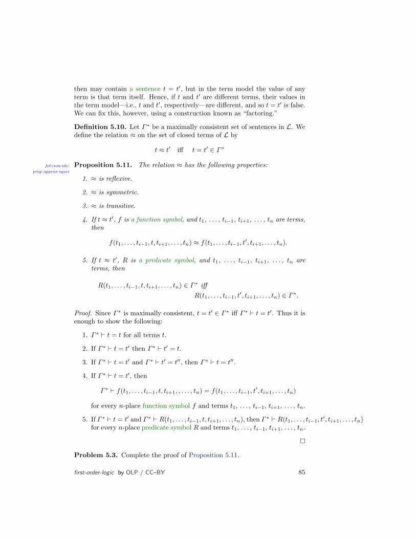
then may contain a sentence t = t′, but in the term model the value of anyterm is that term itself. Hence, if t and t′ are different terms, their values inthe term model—i.e., t and t′, respectively—are different, and so t = t′ is false.We can fix this, however, using a construction known as “factoring.”

Definition 5.10. Let Γ ∗ be a maximally consistent set of sentences in L. Wedefine the relation ≈ on the set of closed terms of L by

t ≈ t′ iff t = t′ ∈ Γ ∗

Proposition 5.11.fol:com:ide:

prop:approx-equiv

The relation ≈ has the following properties:

1. ≈ is reflexive.

2. ≈ is symmetric.

3. ≈ is transitive.

4. If t ≈ t′, f is a function symbol, and t1, . . . , ti−1, ti+1, . . . , tn are terms,then

f(t1, . . . , ti−1, t, ti+1, . . . , tn) ≈ f(t1, . . . , ti−1, t′, ti+1, . . . , tn).

5. If t ≈ t′, R is a predicate symbol, and t1, . . . , ti−1, ti+1, . . . , tn areterms, then

R(t1, . . . , ti−1, t, ti+1, . . . , tn) ∈ Γ ∗ iff

R(t1, . . . , ti−1, t′, ti+1, . . . , tn) ∈ Γ ∗.

Proof. Since Γ ∗ is maximally consistent, t = t′ ∈ Γ ∗ iff Γ ∗ ` t = t′. Thus it isenough to show the following:

1. Γ ∗ ` t = t for all terms t.

2. If Γ ∗ ` t = t′ then Γ ∗ ` t′ = t.

3. If Γ ∗ ` t = t′ and Γ ∗ ` t′ = t′′, then Γ ∗ ` t = t′′.

4. If Γ ∗ ` t = t′, then

Γ ∗ ` f(t1, . . . , ti−1, t, ti+1, , . . . , tn) = f(t1, . . . , ti−1, t′, ti+1, . . . , tn)

for every n-place function symbol f and terms t1, . . . , ti−1, ti+1, . . . , tn.

5. If Γ ∗ ` t = t′ and Γ ∗ ` R(t1, . . . , ti−1, t, ti+1, . . . , tn), then Γ ∗ ` R(t1, . . . , ti−1, t′, ti+1, . . . , tn)

for every n-place predicate symbol R and terms t1, . . . , ti−1, ti+1, . . . , tn.






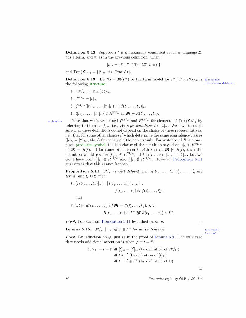
Definition 5.12. Suppose Γ ∗ is a maximally consistent set in a language L,t is a term, and ≈ as in the previous definition. Then:

[t]≈ = t′ : t′ ∈ Trm(L), t ≈ t′

and Trm(L)/≈ = [t]≈ : t ∈ Trm(L).

Definition 5.13. fol:com:ide:

defn:term-model-factor

Let M = M(Γ ∗) be the term model for Γ ∗. Then M/≈ isthe following structure:

1. |M/≈| = Trm(L)/≈.

2. cM/≈ = [c]≈

3. fM/≈([t1]≈, . . . , [tn]≈) = [f(t1, . . . , tn)]≈

4. 〈[t1]≈, . . . , [tn]≈〉 ∈ RM/≈ iff M |= R(t1, . . . , tn).

explanation Note that we have defined fM/≈ and RM/≈ for elements of Trm(L)/≈ byreferring to them as [t]≈, i.e., via representatives t ∈ [t]≈. We have to makesure that these definitions do not depend on the choice of these representatives,i.e., that for some other choices t′ which determine the same equivalence classes([t]≈ = [t′]≈), the definitions yield the same result. For instance, if R is a one-place predicate symbol, the last clause of the definition says that [t]≈ ∈ RM/≈

iff M |= R(t). If for some other term t′ with t ≈ t′, M 6|= R(t), then thedefinition would require [t′]≈ /∈ RM/≈ . If t ≈ t′, then [t]≈ = [t′]≈, but wecan’t have both [t]≈ ∈ RM/≈ and [t]≈ /∈ RM/≈ . However, Proposition 5.11guarantees that this cannot happen.

Proposition 5.14. M/≈ is well defined, i.e., if t1, . . . , tn, t′1, . . . , t′n areterms, and ti ≈ t′i then

1. [f(t1, . . . , tn)]≈ = [f(t′1, . . . , t′n)]≈, i.e.,

f(t1, . . . , tn) ≈ f(t′1, . . . , t′n)

and

2. M |= R(t1, . . . , tn) iff M |= R(t′1, . . . , t′n), i.e.,

R(t1, . . . , tn) ∈ Γ ∗ iff R(t′1, . . . , t′n) ∈ Γ ∗.

Proof. Follows from Proposition 5.11 by induction on n.

Lemma 5.15. fol:com:ide:

lem:truth

M/≈ |= ϕ iff ϕ ∈ Γ ∗ for all sentences ϕ.

Proof. By induction on ϕ, just as in the proof of Lemma 5.9. The only casethat needs additional attention is when ϕ ≡ t = t′.

M/≈ |= t = t′ iff [t]≈ = [t′]≈ (by definition of M/≈)

iff t ≈ t′ (by definition of [t]≈)

iff t = t′ ∈ Γ ∗ (by definition of ≈).





digressionNote that while M(Γ ∗) is always enumerable and infinite, M/≈ may befinite, since it may turn out that there are only finitely many classes [t]≈. Thisis to be expected, since Γ may contain sentences which require any structurein which they are true to be finite. For instance, ∀x∀y x = y is a consistentsentence, but is satisfied only in structures with a domain that contains exactlyone element.

5.8 The Completeness Theorem

fol:com:cth:sec

Let’s combine our results: we arrive at the Godel’s completeness theorem.

Theorem 5.16 (Completeness Theorem).fol:com:cth:

thm:completeness

Let Γ be a set of sentences. If Γis consistent, it is satisfiable.

Proof. Suppose Γ is consistent. By Lemma 5.7, there is a Γ ∗ ⊇ Γ which is max-imally consistent and saturated. If Γ does not contain =, then by Lemma 5.9,M(Γ ∗) |= ϕ iff ϕ ∈ Γ ∗. From this it follows in particular that for all ϕ ∈ Γ ,M(Γ ∗) |= ϕ, so Γ is satisfiable. If Γ does contain =, then by Lemma 5.15,M/≈ |= ϕ iff ϕ ∈ Γ ∗ for all sentences ϕ. In particular, M/≈ |= ϕ for all ϕ ∈ Γ ,so Γ is satisfiable.

Corollary 5.17 (Completeness Theorem, Second Version).fol:com:cth:

cor:completeness

For all Γ and ϕsentences: if Γ ϕ then Γ ` ϕ.

Proof. Note that the Γ ’s in Corollary 5.17 and Theorem 5.16 are universallyquantified. To make sure we do not confuse ourselves, let us restate Theo-rem 5.16 using a different variable: for any set of sentences ∆, if ∆ is con-sistent, it is satisfiable. By contraposition, if ∆ is not satisfiable, then ∆ isinconsistent. We will use this to prove the corollary.

Suppose that Γ ϕ. Then Γ ∪ ¬ϕ is unsatisfiable by Proposition 1.49.Taking Γ ∪ ¬ϕ as our ∆, the previous version of Theorem 5.16 gives us thatΓ ∪ ¬ϕ is inconsistent. By Propositions 3.13 and 4.13, Γ ` ϕ.

Problem 5.4. Use Corollary 5.17 to prove Theorem 5.16, thus showing thatthe two formulations of the completeness theorem are equivalent.

Problem 5.5. In order for a derivation system to be complete, its rules mustbe strong enough to prove every unsatisfiable set inconsistent. Which of therules of LK were necessary to prove completeness? Are any of these rules notused anywhere in the proof? In order to answer these questions, make a list ordiagram that shows which of the rules of LK were used in which results thatlead up to the proof of Theorem 5.16. Be sure to note any tacit uses of rulesin these proofs.





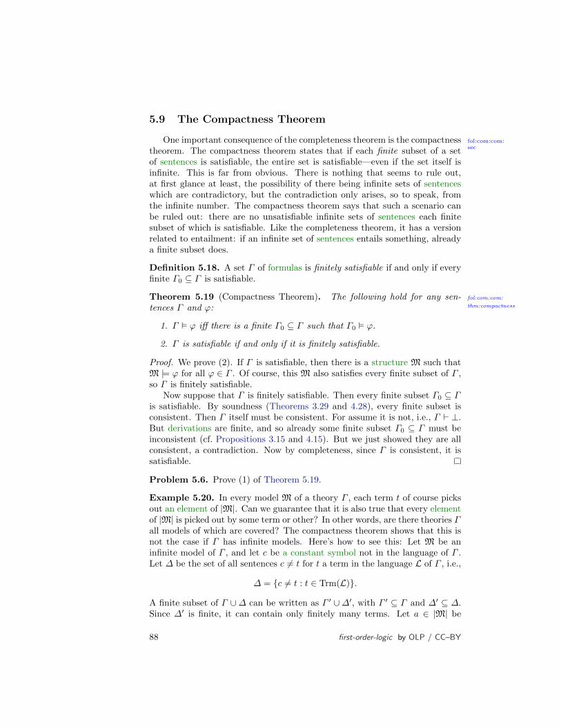
5.9 The Compactness Theorem

fol:com:com:sec

One important consequence of the completeness theorem is the compactnesstheorem. The compactness theorem states that if each finite subset of a setof sentences is satisfiable, the entire set is satisfiable—even if the set itself isinfinite. This is far from obvious. There is nothing that seems to rule out,at first glance at least, the possibility of there being infinite sets of sentenceswhich are contradictory, but the contradiction only arises, so to speak, fromthe infinite number. The compactness theorem says that such a scenario canbe ruled out: there are no unsatisfiable infinite sets of sentences each finitesubset of which is satisfiable. Like the completeness theorem, it has a versionrelated to entailment: if an infinite set of sentences entails something, alreadya finite subset does.

Definition 5.18. A set Γ of formulas is finitely satisfiable if and only if everyfinite Γ0 ⊆ Γ is satisfiable.

Theorem 5.19 (Compactness Theorem). fol:com:com:

thm:compactness

The following hold for any sen-tences Γ and ϕ:

1. Γ ϕ iff there is a finite Γ0 ⊆ Γ such that Γ0 ϕ.

2. Γ is satisfiable if and only if it is finitely satisfiable.

Proof. We prove (2). If Γ is satisfiable, then there is a structure M such thatM |= ϕ for all ϕ ∈ Γ . Of course, this M also satisfies every finite subset of Γ ,so Γ is finitely satisfiable.

Now suppose that Γ is finitely satisfiable. Then every finite subset Γ0 ⊆ Γis satisfiable. By soundness (Theorems 3.29 and 4.28), every finite subset isconsistent. Then Γ itself must be consistent. For assume it is not, i.e., Γ ` ⊥.But derivations are finite, and so already some finite subset Γ0 ⊆ Γ must beinconsistent (cf. Propositions 3.15 and 4.15). But we just showed they are allconsistent, a contradiction. Now by completeness, since Γ is consistent, it issatisfiable.

Problem 5.6. Prove (1) of Theorem 5.19.

Example 5.20. In every model M of a theory Γ , each term t of course picksout an element of |M|. Can we guarantee that it is also true that every elementof |M| is picked out by some term or other? In other words, are there theories Γall models of which are covered? The compactness theorem shows that this isnot the case if Γ has infinite models. Here’s how to see this: Let M be aninfinite model of Γ , and let c be a constant symbol not in the language of Γ .Let ∆ be the set of all sentences c 6= t for t a term in the language L of Γ , i.e.,

∆ = c 6= t : t ∈ Trm(L).

A finite subset of Γ ∪∆ can be written as Γ ′ ∪∆′, with Γ ′ ⊆ Γ and ∆′ ⊆ ∆.Since ∆′ is finite, it can contain only finitely many terms. Let a ∈ |M| be





an element of |M| not picked out by any of them, and let M′ be the structurethat is just like M, but also cM

′= a. Since a 6= ValM(t) for all t occuring

in ∆′, M′ |= ∆′. Since M |= Γ , Γ ′ ⊆ Γ , and c does not occur in Γ , alsoM′ |= Γ ′. Together, M′ |= Γ ′ ∪ ∆′ for every finite subset Γ ′ ∪ ∆′ of Γ ∪ ∆.So every finite subset of Γ ∪∆ is satisfiable. By compactness, Γ ∪∆ itself issatisfiable. So there are models M |= Γ ∪∆. Every such M is a model of Γ ,but is not covered, since ValM(c) 6= ValM(t) for all terms t of L.

Example 5.21. Consider a language L containing the predicate symbol <,constant symbols , , and function symbols +, ×, −, ÷. Let Γ be the setof all sentences in this language true in Q with domain Q and the obviousinterpretations. Γ is the set of all sentences of L true about the rationalnumbers. Of course, in Q (and even in R), there are no numbers which aregreater than 0 but less than 1/k for all k ∈ Z+. Such a number, if it existed,would be an infinitesimal: non-zero, but infinitely small. The compactnesstheorem shows that there are models of Γ in which infinitesimals exist: Let ∆be 0 < c∪c < (÷k) : k ∈ Z+ (where k = (+(+ · · ·+(+) . . . )) withk ’s). For any finite subset ∆0 of ∆ there is a K such that all the sentencesc < k in ∆0 have k < K. If we expand Q to Q′ with cQ

′= 1/K we have

that Q′ |= Γ ∪∆0, and so Γ ∪∆ is finitely satisfiable (Exercise: prove this indetail). By compactness, Γ ∪∆ is satisfiable. Any model S of Γ ∪∆ containsan infinitesimal, namely cS.

Problem 5.7. In the standard model of arithmetic N, there is no element k ∈|N| which satisfies every formula n < x (where n is ′...′ with n ′’s). Usethe compactness theorem to show that the set of sentences in the language ofarithmetic which are true in the standard model of arithmetic N are also truein a structure N′ that contains an element which does satisfy every formulan < x.

Example 5.22. We know that first-order logic with identity predicate canexpress that the size of the domain must have some minimal size: The sen-tence ϕ≥n (which says “there are at least n distinct objects”) is true only instructures where |M| has at least n objects. So if we take

∆ = ϕ≥n : n ≥ 1

then any model of ∆ must be infinite. Thus, we can guarantee that a theoryonly has infinite models by adding ∆ to it: the models of Γ ∪ ∆ are all andonly the infinite models of Γ .

So first-order logic can express infinitude. The compactness theorem showsthat it cannot express finitude, however. For suppose some set of sentences Λwere satisfied in all and only finite structures. Then ∆∪Λ is finitely satisfiable.Why? Suppose ∆′∪Λ′ ⊆ ∆∪Λ is finite with ∆′ ⊆ ∆ and Λ′ ⊆ Λ. Let n be thelargest number such that A≥n ∈ ∆′. Λ, being satisfied in all finite structures,has a model M with finitely many but ≥ n elements. But then M |= ∆′ ∪ Λ′.By compactness, ∆ ∪ Λ has an infinite model, contradicting the assumptionthat Λ is satisfied only in finite structures.





5.10 The Lowenheim-Skolem Theorem

fol:com:dls:sec

The Lowenheim-Skolem Theorem says that if a theory has an infinite model,then it also has a model that is at most denumerable. An immediate consequeneof this fact is that first-order logic cannot express that the size of a structure isnon-enumerable: any sentence or set of sentences satisfied in all non-enumerablestructures is also satisfied in some denumerable structure.

Theorem 5.23. fol:com:dls:

thm:downward-ls

If Γ is consistent then it has a denumerable model, i.e., it issatisfiable in a structure whose domain is either finite or infinite but enumer-able.

Proof. If Γ is consistent, the structure M delivered by the proof of the com-pleteness theorem has a domain |M| whose cardinality is bounded by that ofthe set of the terms of the language L. So M is at most denumerable.

Theorem 5.24. fol:com:dls:

noidentity-ls

If Γ is consistent set of sentences in the language of first-order logic without identity, then it has a denumerable model, i.e., it is satisfi-able in a structure whose domain is infinite and enumerable.

Proof. If Γ is consistent and contains no sentences in which identity appears,then the structure M delivered by the proof of the completness theorem has adomain |M| whose cardinality is identical to that of the set of the terms of thelanguage L. So M is denumerably infinite.

Example 5.25 (Skolem’s Paradox). Zermelo-Fraenkel set theory ZFC is avery powerful framework in which practically all mathematical statements canbe expressed, including facts about the sizes of sets. So for instance, ZFC canprove that the set R of real numbers is non-enumerable, it can prove Cantor’sTheorem that the power set of any set is larger than the set itself, etc. IfZFC is consistent, its models are all infinite, and moreover, they all containelements about which the theory says that they are non-enumerable, such asthe element that makes true the theorem of ZFC that the power set of thenatural numbers exists. By the Lowenheim-Skolem Theorem, ZFC also hasenumerable models—models that contain “non-enumerable” sets but whichthemselves are enumerable.





Chapter 6

Beyond First-order Logic

6.1 Overview

fol:byd:int:sec

First-order logic is not the only system of logic of interest: there are manyextensions and variations of first-order logic. A logic typically consists of theformal specification of a language, usually, but not always, a deductive system,and usually, but not always, an intended semantics. But the technical use ofthe term raises an obvious question: what do logics that are not first-orderlogic have to do with the word “logic,” used in the intuitive or philosophicalsense? All of the systems described below are designed to model reasoning ofsome form or another; can we say what makes them logical?

No easy answers are forthcoming. The word “logic” is used in differentways and in different contexts, and the notion, like that of “truth,” has beenanalyzed from numerous philosophical stances. For example, one might takethe goal of logical reasoning to be the determination of which statements arenecessarily true, true a priori, true independent of the interpretation of thenonlogical terms, true by virtue of their form, or true by linguistic convention;and each of these conceptions requires a good deal of clarification. Even ifone restricts one’s attention to the kind of logic used in mathematics, there islittle agreement as to its scope. For example, in the Principia Mathematica,Russell and Whitehead tried to develop mathematics on the basis of logic,in the logicist tradition begun by Frege. Their system of logic was a formof higher-type logic similar to the one described below. In the end they wereforced to introduce axioms which, by most standards, do not seem purely logical(notably, the axiom of infinity, and the axiom of reducibility), but one mightnonetheless hold that some forms of higher-order reasoning should be acceptedas logical. In contrast, Quine, whose ontology does not admit “propositions”as legitimate objects of discourse, argues that second-order and higher-orderlogic are really manifestations of set theory in sheep’s clothing; in other words,systems involving quantification over predicates are not purely logical.

For now, it is best to leave such philosophical issues for a rainy day, andsimply think of the systems below as formal idealizations of various kinds of

91

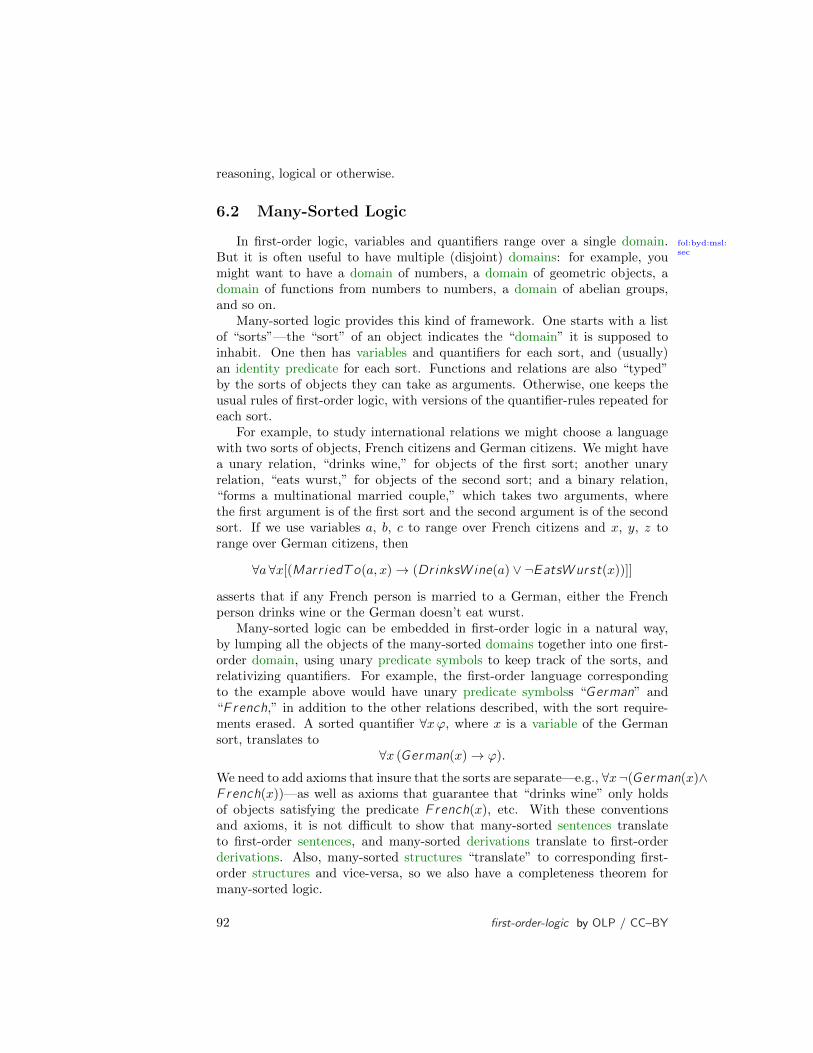
reasoning, logical or otherwise.

6.2 Many-Sorted Logic

fol:byd:msl:sec

In first-order logic, variables and quantifiers range over a single domain.But it is often useful to have multiple (disjoint) domains: for example, youmight want to have a domain of numbers, a domain of geometric objects, adomain of functions from numbers to numbers, a domain of abelian groups,and so on.

Many-sorted logic provides this kind of framework. One starts with a listof “sorts”—the “sort” of an object indicates the “domain” it is supposed toinhabit. One then has variables and quantifiers for each sort, and (usually)an identity predicate for each sort. Functions and relations are also “typed”by the sorts of objects they can take as arguments. Otherwise, one keeps theusual rules of first-order logic, with versions of the quantifier-rules repeated foreach sort.

For example, to study international relations we might choose a languagewith two sorts of objects, French citizens and German citizens. We might havea unary relation, “drinks wine,” for objects of the first sort; another unaryrelation, “eats wurst,” for objects of the second sort; and a binary relation,“forms a multinational married couple,” which takes two arguments, wherethe first argument is of the first sort and the second argument is of the secondsort. If we use variables a, b, c to range over French citizens and x, y, z torange over German citizens, then

∀a∀x[(Marr iedTo(a, x)→ (DrinksW ine(a) ∨ ¬EatsWurst(x))]]

asserts that if any French person is married to a German, either the Frenchperson drinks wine or the German doesn’t eat wurst.

Many-sorted logic can be embedded in first-order logic in a natural way,by lumping all the objects of the many-sorted domains together into one first-order domain, using unary predicate symbols to keep track of the sorts, andrelativizing quantifiers. For example, the first-order language correspondingto the example above would have unary predicate symbolss “German” and“F rench,” in addition to the other relations described, with the sort require-ments erased. A sorted quantifier ∀xϕ, where x is a variable of the Germansort, translates to

∀x (German(x)→ ϕ).

We need to add axioms that insure that the sorts are separate—e.g., ∀x¬(German(x)∧F rench(x))—as well as axioms that guarantee that “drinks wine” only holdsof objects satisfying the predicate F rench(x), etc. With these conventionsand axioms, it is not difficult to show that many-sorted sentences translateto first-order sentences, and many-sorted derivations translate to first-orderderivations. Also, many-sorted structures “translate” to corresponding first-order structures and vice-versa, so we also have a completeness theorem formany-sorted logic.





6.3 Second-Order logic

fol:byd:sol:sec

The language of second-order logic allows one to quantify not just over adomain of individuals, but over relations on that domain as well. Given afirst-order language L, for each k one adds variables R which range over k-aryrelations, and allows quantification over those variables. If R is a variable fora k-ary relation, and t1, . . . , tk are ordinary (first-order) terms, R(t1, . . . , tk)is an atomic formula. Otherwise, the set of formulas is defined just as in thecase of first-order logic, with additional clauses for second-order quantification.Note that we only have the identity predicate for first-order terms: if R andS are relation variables of the same arity k, we can define R = S to be anabbreviation for

∀x1 . . . ∀xk (R(x1, . . . , xk)↔ S(x1, . . . , xk)).

The rules for second-order logic simply extend the quantifier rules to thenew second order variables. Here, however, one has to be a little bit careful toexplain how these variables interact with the predicate symbols of L, and withformulas of L more generally. At the bare minimum, relation variables countas terms, so one has inferences of the form

ϕ(R) ` ∃Rϕ(R)

But if L is the language of arithmetic with a constant relation symbol <, onewould also expect the following inference to be valid:

x < y ` ∃RR(x, y)

or for a given formula ϕ,

ϕ(x1, . . . , xk) ` ∃RR(x1, . . . , xk)

More generally, we might want to allow inferences of the form

ϕ[λ~x. ψ(~x)/R] ` ∃Rϕ

where ϕ[λ~x. ψ(~x)/R] denotes the result of replacing every atomic formula ofthe form Rt1, . . . , tk in ϕ by ψ(t1, . . . , tk). This last rule is equivalent to havinga comprehension schema, i.e., an axiom of the form

∃R ∀x1, . . . , xk (ϕ(x1, . . . , xk)↔ R(x1, . . . , xk)),

one for each formula ϕ in the second-order language, in which R is not a freevariable. (Exercise: show that if R is allowed to occur in ϕ, this schema isinconsistent!)

When logicians refer to the “axioms of second-order logic” they usuallymean the minimal extension of first-order logic by second-order quantifier rulestogether with the comprehension schema. But it is often interesting to studyweaker subsystems of these axioms and rules. For example, note that in its full





generality the axiom schema of comprehension is impredicative: it allows one toassert the existence of a relation R(x1, . . . , xk) that is “defined” by a formulawith second-order quantifiers; and these quantifiers range over the set of allsuch relations—a set which includes R itself! Around the turn of the twentiethcentury, a common reaction to Russell’s paradox was to lay the blame on suchdefinitions, and to avoid them in developing the foundations of mathematics.If one prohibits the use of second-order quantifiers in the formula ϕ, one has apredicative form of comprehension, which is somewhat weaker.

From the semantic point of view, one can think of a second-order structureas consisting of a first-order structure for the language, coupled with a set ofrelations on the domain over which the second-order quantifiers range (moreprecisely, for each k there is a set of relations of arity k). Of course, if compre-hension is included in the proof system, then we have the added requirementthat there are enough relations in the “second-order part” to satisfy the com-prehension axioms—otherwise the proof system is not sound! One easy wayto insure that there are enough relations around is to take the second-orderpart to consist of all the relations on the first-order part. Such a structure iscalled full, and, in a sense, is really the “intended structure” for the language.If we restrict our attention to full structures we have what is known as thefull second-order semantics. In that case, specifying a structure boils downto specifying the first-order part, since the contents of the second-order partfollow from that implicitly.

To summarize, there is some ambiguity when talking about second-orderlogic. In terms of the proof system, one might have in mind either

1. A “minimal” second-order proof system, together with some comprehen-sion axioms.

2. The “standard” second-order proof system, with full comprehension.

In terms of the semantics, one might be interested in either

1. The “weak” semantics, where a structure consists of a first-order part,together with a second-order part big enough to satisfy the comprehensionaxioms.

2. The “standard” second-order semantics, in which one considers full struc-tures only.

When logicians do not specify the proof system or the semantics they have inmind, they are usually refering to the second item on each list. The advantageto using this semantics is that, as we will see, it gives us categorical descriptionsof many natural mathematical structures; at the same time, the proof systemis quite strong, and sound for this semantics. The drawback is that the proofsystem is not complete for the semantics; in fact, no effectively given proofsystem is complete for the full second-order semantics. On the other hand, wewill see that the proof system is complete for the weakened semantics; this





implies that if a sentence is not provable, then there is some structure, notnecessarily the full one, in which it is false.

The language of second-order logic is quite rich. One can identify unaryrelations with subsets of the domain, and so in particular you can quantify overthese sets; for example, one can express induction for the natural numbers witha single axiom

∀R ((R() ∧ ∀x (R(x)→ R(x′)))→ ∀xR(x)).

If one takes the language of arithmetic to have symbols , ′,+,× and <, onecan add the following axioms to describe their behavior:

1. ∀x¬x′ =

2. ∀x ∀y (s(x) = s(y)→ x = y)

3. ∀x (x+ ) = x

4. ∀x∀y (x+ y′) = (x+ y)′

5. ∀x (x× ) =

6. ∀x∀y (x× y′) = ((x× y) + x)

7. ∀x∀y (x < y ↔ ∃z y = (x+ z′))

It is not difficult to show that these axioms, together with the axiom of induc-tion above, provide a categorical description of the structure N, the standardmodel of arithmetic, provided we are using the full second-order semantics.Given any structure A in which these axioms are true, define a function f fromN to the domain of A using ordinary recursion on N, so that f(0) = A andf(x+ 1) = ′A(f(x)). Using ordinary induction on N and the fact that axioms(1) and (2) hold in A, we see that f is injective. To see that f is surjective, letP be the set of elements of |A| that are in the range of f . Since A is full, P is inthe second-order domain. By the construction of f , we know that A is in P ,and that P is closed under ′A. The fact that the induction axiom holds in A (inparticular, for P ) guarantees that P is equal to the entire first-order domainof A. This shows that f is a bijection. Showing that f is a homomorphism isno more difficult, using ordinary induction on N repeatedly.

In set-theoretic terms, a function is just a special kind of relation; for ex-ample, a unary function f can be identified with a binary relation R satisfying∀x ∃y R(x, y). As a result, one can quantify over functions too. Using the fullsemantics, one can then define the class of infinite structures to be the class ofstructures A for which there is an injective function from the domain of A toa proper subset of itself:

∃f (∀x ∀y (f(x) = f(y)→ x = y) ∧ ∃y ∀x f(x) 6= y).

The negation of this sentence then defines the class of finite structures.





In addition, one can define the class of well-orderings, by adding the follow-ing to the definition of a linear ordering:

∀P (∃xP (x)→ ∃x (P (x) ∧ ∀y (y < x→ ¬P (y)))).

This asserts that every non-empty set has a least element, modulo the identifi-cation of “set” with “one-place relation”. For another example, one can expressthe notion of connectedness for graphs, by saying that there is no nontrivialseparation of the vertices into disconnected parts:

¬∃A (∃xA(x) ∧ ∃y ¬A(y) ∧ ∀w ∀z ((A(w) ∧ ¬A(z))→ ¬R(w, z))).

For yet another example, you might try as an exercise to define the class offinite structures whose domain has even size. More strikingly, one can pro-vide a categorical description of the real numbers as a complete ordered fieldcontaining the rationals.

In short, second-order logic is much more expressive than first-order logic.That’s the good news; now for the bad. We have already mentioned that thereis no effective proof system that is complete for the full second-order semantics.For better or for worse, many of the properties of first-order logic are absent,including compactness and the Lowenheim-Skolem theorems.

On the other hand, if one is willing to give up the full second-order seman-tics in terms of the weaker one, then the minimal second-order proof systemis complete for this semantics. In other words, if we read ` as “proves inthe minimal system” and as “logically implies in the weaker semantics”, wecan show that whenever Γ ϕ then Γ ` ϕ. If one wants to include specificcomprehension axioms in the proof system, one has to restrict the semanticsto second-order structures that satisfy these axioms: for example, if ∆ con-sists of a set of comprehension axioms (possibly all of them), we have thatif Γ ∪ ∆ ϕ, then Γ ∪ ∆ ` ϕ. In particular, if ϕ is not provable using thecomprehension axioms we are considering, then there is a model of ¬ϕ in whichthese comprehension axioms nonetheless hold.

The easiest way to see that the completeness theorem holds for the weakersemantics is to think of second-order logic as a many-sorted logic, as follows.One sort is interpreted as the ordinary “first-order” domain, and then for eachk we have a domain of “relations of arity k.” We take the language to havebuilt-in relation symbols “truek(R, x1, . . . , xk)” which is meant to assert thatR holds of x1, . . . , xk, where R is a variable of the sort “k-ary relation” andx1, . . . , xk are objects of the first-order sort.

With this identification, the weak second-order semantics is essentially theusual semantics for many-sorted logic; and we have already observed thatmany-sorted logic can be embedded in first-order logic. Modulo the trans-lations back and forth, then, the weaker conception of second-order logic isreally a form of first-order logic in disguise, where the domain contains both“objects” and “relations” governed by the appropriate axioms.





6.4 Higher-Order logic

fol:byd:hol:sec

Passing from first-order logic to second-order logic enabled us to talk aboutsets of objects in the first-order domain, within the formal language. Why stopthere? For example, third-order logic should enable us to deal with sets of setsof objects, or perhaps even sets which contain both objects and sets of objects.And fourth-order logic will let us talk about sets of objects of that kind. Asyou may have guessed, one can iterate this idea arbitrarily.

In practice, higher-order logic is often formulated in terms of functions in-stead of relations. (Modulo the natural identifications, this difference is inessen-tial.) Given some basic “sorts” A, B, C, . . . (which we will now call “types”),we can create new ones by stipulating

If σ and τ are finite types then so is σ → τ .

Think of types as syntactic “labels,” which classify the objects we want in ourdomain; σ → τ describes those objects that are functions which take objectsof type σ to objects of type τ . For example, we might want to have a typeΩ of truth values, “true” and “false,” and a type N of natural numbers. Inthat case, you can think of objects of type N → Ω as unary relations, orsubsets of N; objects of type N → N are functions from natural numers tonatural numbers; and objects of type (N→ N)→ N are “functionals,” that is,higher-type functions that take functions to numbers.

As in the case of second-order logic, one can think of higher-order logic as akind of many-sorted logic, where there is a sort for each type of object we wantto consider. But it is usually clearer just to define the syntax of higher-typelogic from the ground up. For example, we can define a set of finite typesinductively, as follows:

1. N is a finite type.

2. If σ and τ are finite types, then so is σ → τ .

3. If σ and τ are finite types, so is σ × τ .

Intuitively, N denotes the type of the natural numbers, σ → τ denotes thetype of functions from σ to τ , and σ × τ denotes the type of pairs of objects,one from σ and one from τ . We can then define a set of terms inductively, asfollows:

1. For each type σ, there is a stock of variables x, y, z, . . . of type σ

2. is a term of type N

3. S (successor) is a term of type N→ N

4. If s is a term of type σ, and t is a term of type N → (σ → σ), then Rstis a term of type N→ σ





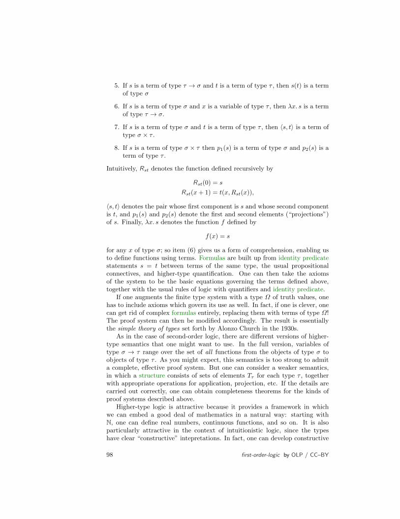
5. If s is a term of type τ → σ and t is a term of type τ , then s(t) is a termof type σ

6. If s is a term of type σ and x is a variable of type τ , then λx. s is a termof type τ → σ.

7. If s is a term of type σ and t is a term of type τ , then 〈s, t〉 is a term oftype σ × τ .

8. If s is a term of type σ × τ then p1(s) is a term of type σ and p2(s) is aterm of type τ .

Intuitively, Rst denotes the function defined recursively by

Rst(0) = s

Rst(x+ 1) = t(x,Rst(x)),

〈s, t〉 denotes the pair whose first component is s and whose second componentis t, and p1(s) and p2(s) denote the first and second elements (“projections”)of s. Finally, λx. s denotes the function f defined by

f(x) = s

for any x of type σ; so item (6) gives us a form of comprehension, enabling usto define functions using terms. Formulas are built up from identity predicatestatements s = t between terms of the same type, the usual propositionalconnectives, and higher-type quantification. One can then take the axiomsof the system to be the basic equations governing the terms defined above,together with the usual rules of logic with quantifiers and identity predicate.

If one augments the finite type system with a type Ω of truth values, onehas to include axioms which govern its use as well. In fact, if one is clever, onecan get rid of complex formulas entirely, replacing them with terms of type Ω!The proof system can then be modified accordingly. The result is essentiallythe simple theory of types set forth by Alonzo Church in the 1930s.

As in the case of second-order logic, there are different versions of higher-type semantics that one might want to use. In the full version, variables oftype σ → τ range over the set of all functions from the objects of type σ toobjects of type τ . As you might expect, this semantics is too strong to admita complete, effective proof system. But one can consider a weaker semantics,in which a structure consists of sets of elements Tτ for each type τ , togetherwith appropriate operations for application, projection, etc. If the details arecarried out correctly, one can obtain completeness theorems for the kinds ofproof systems described above.

Higher-type logic is attractive because it provides a framework in whichwe can embed a good deal of mathematics in a natural way: starting withN, one can define real numbers, continuous functions, and so on. It is alsoparticularly attractive in the context of intuitionistic logic, since the typeshave clear “constructive” intepretations. In fact, one can develop constructive





versions of higher-type semantics (based on intuitionistic, rather than classicallogic) that clarify these constructive interpretations quite nicely, and are, inmany ways, more interesting than the classical counterparts.

6.5 Intuitionistic Logic

fol:byd:il:sec

In constrast to second-order and higher-order logic, intuitionistic first-orderlogic represents a restriction of the classical version, intended to model a more“constructive” kind of reasoning. The following examples may serve to illus-trate some of the underlying motivations.

Suppose someone came up to you one day and announced that they haddetermined a natural number x, with the property that if x is prime, theRiemann hypothesis is true, and if x is composite, the Riemann hypothesis isfalse. Great news! Whether the Riemann hypothesis is true or not is one ofthe big open questions of mathematics, and here they seem to have reducedthe problem to one of calculation, that is, to the determination of whether aspecific number is prime or not.

What is the magic value of x? They describe it as follows: x is the naturalnumber that is equal to 7 if the Riemann hypothesis is true, and 9 otherwise.

Angrily, you demand your money back. From a classical point of view, thedescription above does in fact determine a unique value of x; but what youreally want is a value of x that is given explicitly.

To take another, perhaps less contrived example, consider the followingquestion. We know that it is possible to raise an irrational number to a rational

power, and get a rational result. For example,√

22

= 2. What is less clearis whether or not it is possible to raise an irrational number to an irrationalpower, and get a rational result. The following theorem answers this in theaffirmative:

Theorem 6.1. There are irrational numbers a and b such that ab is rational.

Proof. Consider√

2√2. If this is rational, we are done: we can let a = b =

√2.

Otherwise, it is irrational. Then we have

(√

2

√2)√2 =√

2

√2·√2

=√

22

= 2,

which is certainly rational. So, in this case, let a be√

2√2, and let b be

√2.

Does this constitute a valid proof? Most mathematicians feel that it does.But again, there is something a little bit unsatisfying here: we have provedthe existence of a pair of real numbers with a certain property, without beingable to say which pair of numbers it is. It is possible to prove the same result,but in such a way that the pair a, b is given in the proof: take a =

√3 and

b = log3 4. Then

ab =√

3log3 4

= 31/2·log3 4 = (3log3 4)1/2 = 41/2 = 2,





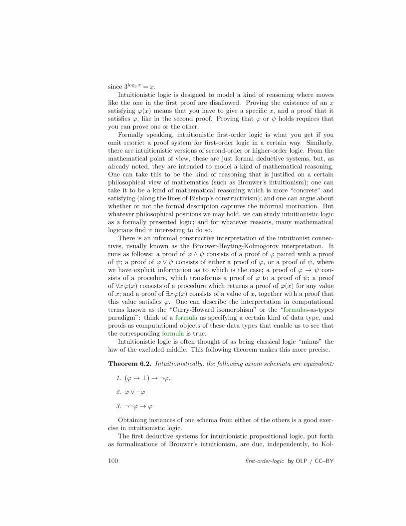
since 3log3 x = x.Intuitionistic logic is designed to model a kind of reasoning where moves

like the one in the first proof are disallowed. Proving the existence of an xsatisfying ϕ(x) means that you have to give a specific x, and a proof that itsatisfies ϕ, like in the second proof. Proving that ϕ or ψ holds requires thatyou can prove one or the other.

Formally speaking, intuitionistic first-order logic is what you get if youomit restrict a proof system for first-order logic in a certain way. Similarly,there are intuitionistic versions of second-order or higher-order logic. From themathematical point of view, these are just formal deductive systems, but, asalready noted, they are intended to model a kind of mathematical reasoning.One can take this to be the kind of reasoning that is justified on a certainphilosophical view of mathematics (such as Brouwer’s intuitionism); one cantake it to be a kind of mathematical reasoning which is more “concrete” andsatisfying (along the lines of Bishop’s constructivism); and one can argue aboutwhether or not the formal description captures the informal motivation. Butwhatever philosophical positions we may hold, we can study intuitionistic logicas a formally presented logic; and for whatever reasons, many mathematicallogicians find it interesting to do so.

There is an informal constructive interpretation of the intuitionist connec-tives, usually known as the Brouwer-Heyting-Kolmogorov interpretation. Itruns as follows: a proof of ϕ ∧ ψ consists of a proof of ϕ paired with a proofof ψ; a proof of ϕ ∨ ψ consists of either a proof of ϕ, or a proof of ψ, wherewe have explicit information as to which is the case; a proof of ϕ → ψ con-sists of a procedure, which transforms a proof of ϕ to a proof of ψ; a proofof ∀xϕ(x) consists of a procedure which returns a proof of ϕ(x) for any valueof x; and a proof of ∃xϕ(x) consists of a value of x, together with a proof thatthis value satisfies ϕ. One can describe the interpretation in computationalterms known as the “Curry-Howard isomorphism” or the “formulas-as-typesparadigm”: think of a formula as specifying a certain kind of data type, andproofs as computational objects of these data types that enable us to see thatthe corresponding formula is true.

Intuitionistic logic is often thought of as being classical logic “minus” thelaw of the excluded middle. This following theorem makes this more precise.

Theorem 6.2. Intuitionistically, the following axiom schemata are equivalent:

1. (ϕ→ ⊥)→ ¬ϕ.

2. ϕ ∨ ¬ϕ

3. ¬¬ϕ→ ϕ

Obtaining instances of one schema from either of the others is a good exer-cise in intuitionistic logic.

The first deductive systems for intuitionistic propositional logic, put forthas formalizations of Brouwer’s intuitionism, are due, independently, to Kol-





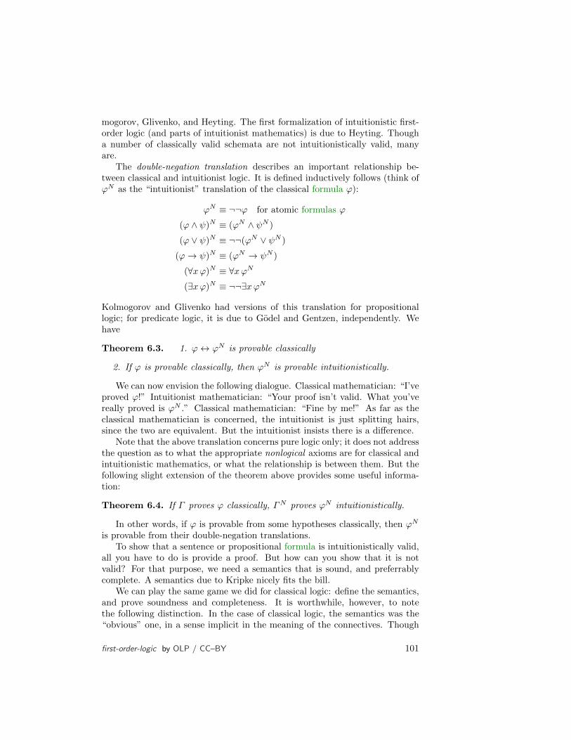
mogorov, Glivenko, and Heyting. The first formalization of intuitionistic first-order logic (and parts of intuitionist mathematics) is due to Heyting. Thougha number of classically valid schemata are not intuitionistically valid, manyare.

The double-negation translation describes an important relationship be-tween classical and intuitionist logic. It is defined inductively follows (think ofϕN as the “intuitionist” translation of the classical formula ϕ):

ϕN ≡ ¬¬ϕ for atomic formulas ϕ

(ϕ ∧ ψ)N ≡ (ϕN ∧ ψN )

(ϕ ∨ ψ)N ≡ ¬¬(ϕN ∨ ψN )

(ϕ→ ψ)N ≡ (ϕN → ψN )

(∀xϕ)N ≡ ∀xϕN

(∃xϕ)N ≡ ¬¬∃xϕN

Kolmogorov and Glivenko had versions of this translation for propositionallogic; for predicate logic, it is due to Godel and Gentzen, independently. Wehave

Theorem 6.3. 1. ϕ↔ ϕN is provable classically

2. If ϕ is provable classically, then ϕN is provable intuitionistically.

We can now envision the following dialogue. Classical mathematician: “I’veproved ϕ!” Intuitionist mathematician: “Your proof isn’t valid. What you’vereally proved is ϕN .” Classical mathematician: “Fine by me!” As far as theclassical mathematician is concerned, the intuitionist is just splitting hairs,since the two are equivalent. But the intuitionist insists there is a difference.

Note that the above translation concerns pure logic only; it does not addressthe question as to what the appropriate nonlogical axioms are for classical andintuitionistic mathematics, or what the relationship is between them. But thefollowing slight extension of the theorem above provides some useful informa-tion:

Theorem 6.4. If Γ proves ϕ classically, ΓN proves ϕN intuitionistically.

In other words, if ϕ is provable from some hypotheses classically, then ϕN

is provable from their double-negation translations.To show that a sentence or propositional formula is intuitionistically valid,

all you have to do is provide a proof. But how can you show that it is notvalid? For that purpose, we need a semantics that is sound, and preferrablycomplete. A semantics due to Kripke nicely fits the bill.

We can play the same game we did for classical logic: define the semantics,and prove soundness and completeness. It is worthwhile, however, to notethe following distinction. In the case of classical logic, the semantics was the“obvious” one, in a sense implicit in the meaning of the connectives. Though





one can provide some intuitive motivation for Kripke semantics, the latter doesnot offer the same feeling of inevitability. In addition, the notion of a classicalstructure is a natural mathematical one, so we can either take the notion of astructure to be a tool for studying classical first-order logic, or take classicalfirst-order logic to be a tool for studying mathematical structures. In contrast,Kripke structures can only be viewed as a logical construct; they don’t seemto have independent mathematical interest.

A Kripke structure for a propositional langauge consists of a partial orderMod(P ) with a least element, and an “monotone” assignment of propositionalvariables to the elements of Mod(P ). The intuition is that the elements ofMod(P ) represent “worlds,” or “states of knowledge”; an element p ≥ q rep-resents a “possible future state” of q; and the propositional variables assignedto p are the propositions that are known to be true in state p. The forcingrelation P, p ϕ then extends this relationship to arbitrary formulas in thelanguage; read P, p ϕ as “ϕ is true in state p.” The relationship is definedinductively, as follows:

1. P, p pi iff pi is one of the propositional variables assigned to p.

2. P, p 1 ⊥.

3. P, p (ϕ ∧ ψ) iff P, p ϕ and P, p ψ.

4. P, p (ϕ ∨ ψ) iff P, p ϕ or P, p ψ.

5. P, p (ϕ→ ψ) iff, whenever q ≥ p and P, q ϕ, then P, q ψ.

It is a good exercise to try to show that ¬(p∧ q)→ (¬p∨¬q) is not intuitionis-tically valid, by cooking up a Kripke structure that provides a counterexample.

6.6 Modal Logics

fol:byd:mod:sec

Consider the following example of a conditional sentence:

If Jeremy is alone in that room, then he is drunk and naked anddancing on the chairs.

This is an example of a conditional assertion that may be materially truebut nonetheless misleading, since it seems to suggest that there is a strongerlink between the antecedent and conclusion other than simply that either theantecedent is false or the consequent true. That is, the wording suggests thatthe claim is not only true in this particular world (where it may be trivially true,because Jeremy is not alone in the room), but that, moreover, the conclusionwould have been true had the antecedent been true. In other words, one cantake the assertion to mean that the claim is true not just in this world, but inany “possible” world; or that it is necessarily true, as opposed to just true inthis particular world.





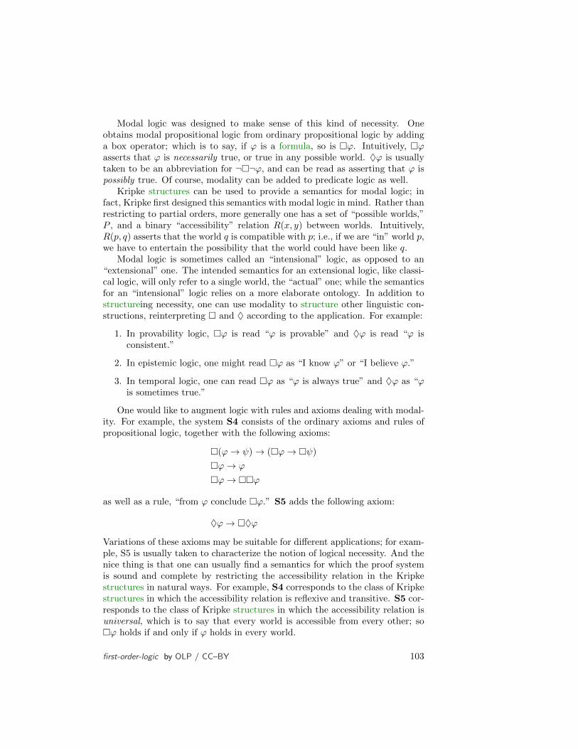
Modal logic was designed to make sense of this kind of necessity. Oneobtains modal propositional logic from ordinary propositional logic by addinga box operator; which is to say, if ϕ is a formula, so is ϕ. Intuitively, ϕasserts that ϕ is necessarily true, or true in any possible world. ♦ϕ is usuallytaken to be an abbreviation for ¬¬ϕ, and can be read as asserting that ϕ ispossibly true. Of course, modality can be added to predicate logic as well.

Kripke structures can be used to provide a semantics for modal logic; infact, Kripke first designed this semantics with modal logic in mind. Rather thanrestricting to partial orders, more generally one has a set of “possible worlds,”P , and a binary “accessibility” relation R(x, y) between worlds. Intuitively,R(p, q) asserts that the world q is compatible with p; i.e., if we are “in” world p,we have to entertain the possibility that the world could have been like q.

Modal logic is sometimes called an “intensional” logic, as opposed to an“extensional” one. The intended semantics for an extensional logic, like classi-cal logic, will only refer to a single world, the “actual” one; while the semanticsfor an “intensional” logic relies on a more elaborate ontology. In addition tostructureing necessity, one can use modality to structure other linguistic con-structions, reinterpreting and ♦ according to the application. For example:

1. In provability logic, ϕ is read “ϕ is provable” and ♦ϕ is read “ϕ isconsistent.”

2. In epistemic logic, one might read ϕ as “I know ϕ” or “I believe ϕ.”

3. In temporal logic, one can read ϕ as “ϕ is always true” and ♦ϕ as “ϕis sometimes true.”

One would like to augment logic with rules and axioms dealing with modal-ity. For example, the system S4 consists of the ordinary axioms and rules ofpropositional logic, together with the following axioms:

(ϕ→ ψ)→ (ϕ→ ψ)

ϕ→ ϕ

ϕ→ ϕ

as well as a rule, “from ϕ conclude ϕ.” S5 adds the following axiom:

♦ϕ→ ♦ϕ

Variations of these axioms may be suitable for different applications; for exam-ple, S5 is usually taken to characterize the notion of logical necessity. And thenice thing is that one can usually find a semantics for which the proof systemis sound and complete by restricting the accessibility relation in the Kripkestructures in natural ways. For example, S4 corresponds to the class of Kripkestructures in which the accessibility relation is reflexive and transitive. S5 cor-responds to the class of Kripke structures in which the accessibility relation isuniversal, which is to say that every world is accessible from every other; soϕ holds if and only if ϕ holds in every world.





6.7 Other Logics

fol:byd:oth:sec

As you may have gathered by now, it is not hard to design a new logic. Youtoo can create your own a syntax, make up a deductive system, and fashiona semantics to go with it. You might have to be a bit clever if you want theproof system to be complete for the semantics, and it might take some effort toconvince the world at large that your logic is truly interesting. But, in return,you can enjoy hours of good, clean fun, exploring your logic’s mathematicaland computational properties.

Recent decades have witnessed a veritable explosion of formal logics. Fuzzylogic is designed to model reasoning about vague properties. Probabilistic logicis designed to model reasoning about uncertainty. Default logics and nonmono-tonic logics are designed to model defeasible forms of reasoning, which is to say,“reasonable” inferences that can later be overturned in the face of new informa-tion. There are epistemic logics, designed to model reasoning about knowledge;causal logics, designed to model reasoning about causal relationships; and even“deontic” logics, which are designed to model reasoning about moral and ethi-cal obligations. Depending on whether the primary motivation for introducingthese systems is philosophical, mathematical, or computational, you may findsuch creatures studies under the rubric of mathematical logic, philosophicallogic, artificial intelligence, cognitive science, or elsewhere.

The list goes on and on, and the possibilities seem endless. We may neverattain Leibniz’ dream of reducing all of human reason to calculation—but thatcan’t stop us from trying.

Photo Credits

104

Bibliography

105

first-order logic - university of...

Documents