Firm-to-Firm Matching Along the Global Supply Chain∗

Raluca Dragusanu†

12 May 2014

(Preliminary and Incomplete)

Abstract: Despite its importance for international trade, our under-standing of the matching process between importing and exportingfirms remains limited. To shed light on this question, I use confidentialU.S. customs data to match firm-level information of Indian manu-facturing exporters from the CMIE-Prowess database with firm-levelinformation of their U.S. importers from the Census Longitudinal Busi-ness Database. I develop a model of sequential production in whichbuyers (importers) engage in costly search for suppliers (exporters)to control a production stage and optimally decide the amount ofinvestment in search. The model shows that the marginal benefit ofassigning a high-capability supplier to a given stage increases with thedownstreamness of the stage of production, and relatively more whenthe final product is less differentiated. Focusing on firm size as a proxyfor firm capability, the matched data highlights three key facts that areconsistent with the model predictions and are robust to different em-pirical strategies. First, there is positive assortative matching betweenU.S. buyers and their Indian suppliers. The elasticity of average buyersize with respect to Indian firm size is around 0.2. Second, the strengthof positive matching increases with the proximity to final use of theproduct traded (downstreamness). The magnitude of the buyer sizeelasticity is 0.5 when Indian firms supply final products to U.S. firms,and close to zero when they supply intermediate products. Finally,matching is stronger - and more sensitive to downstreamness - whenthe demand elasticity faced by the U.S. buyer is high.

JEL Classification: F1, F6, F10, F14, L6

Keywords: Heterogeneous firms, buyer-supplier relationships, globalsupply chains, assortative matching

∗I am grateful to my advisers Pol Antràs, Marc Melitz, Nathan Nunn for their guidance and support. I thankJonathan Fisher for his extensive help with the Census data. I also thank Allan Collard-Wexler, Dominic Wilson,Mary Amiti, Itzik Fadlon, Benjamin Mandel, Francisco Queiro, and seminar participants for valuable suggestions.The research in this paper was conducted while the author was a Special Sworn Status researcher of the U.S. CensusBureau at the Boston and New York Research Data Centers. Any opinions and conclusions expressed herein are thoseof the author and do not necessarily represent the views of the U.S. Census Bureau. All results have been reviewed toensure that no confidential information is disclosed.

†Harvard University. E-mail:rdragus@fas.harvard.edu; Website: http://scholar.harvard.edu/rdragusanu.

1

1. Introduction

Every year, US firms engage in import transactions with more than one million firms from aroundthe world. Together, these transactions span more than one and half million pairs of buyer-supplier relationships. These numbers have grown sharply over the last 20 years. Falling tradecosts and improved supply chain management technology have led US firms to outsource parts ofthe production chain to developing countries. Firms in these countries now perform tasks at manydifferent stages along the global supply chain from the production of basic inputs to complexassembly of parts and manufacturing of final goods. Production fragmentation has contributedto a large increase in the share of US imports from developing countries, from around 28 percentin 1990 to 56 percent in 2012.

As a result, the matching between US buyers and their suppliers in developing countries hasbecome an increasingly important activity for both sides. US buyers invest substantial resourcesin supplier selection and monitoring to ensure suppliers meet their requirements. Supplier failurecan be very costly as shortages of parts cause production delays and quality defects can lead torecalls1. For developing country firms, relationships with buyers in developed countries providenot only market access, but also constitute an important channel to access new technologies,management practices and demand information (Egan and Mody, 1992).

Although the matching between buyers and suppliers plays an important role in internationaltransactions, our understanding of this matching process remains limited. In large part, this isbecause data that allows us to observe detailed information about firms on both sides is noteasily available. To shed light on this question, I construct a novel dataset, which links firm-levelinformation on Indian manufacturing exporters from the CMIE-Prowess database with firm-levelinformation on the US firms with whom they engage in trade. To create these matches I usethe US import customs transactions from the US Census confidential Linked/Longitudinal FirmTrade Transaction Database (LFTTD). I investigate whether high-performing (large) US firmsmatch with high-performing (large) Indian firms and whether that varies systematically with theposition in the supply chain of the Indian firm.

I illustrate the intuition underlying the matching between buyers and suppliers along the pro-duction chain in a model of sequential production featuring complementarities. The productionof a final good entails the completion of a number of sequential stages. A buying firm (buyer)is in charge of organizing the production of the final good along the value chain. Each stage ofproduction m is controlled by a single supplier who uses the value of production up to stage m− 1as an input into stage m production process. Buyers and suppliers are heterogeneous in theircapability. The stage revenue function features complementarities between the the capabilitiesof the buying firm and of the supplier controlling the stage. At each stage, buyers optimallychoose the investments in search for high-capability suppliers to control the production process.A key feature of the model is that the marginal contribution to revenue of the stage-m supplieris increasing with the stage of production m. This implies that the marginal benefit of searchfor the high-capability supplier increases with the stage of production. The model delivers three

1See Beil (2010) for a comprehensive discussion of the process of supplier selection.

main predictions. The optimal amount of investment in supplier search, and hence the strengthof positive assortative matching between buyers and suppliers increases with (1) the stage ofproduction; (2) the elasticity of demand faced by the buyer; (3) the stage of production relativelymore when the buyer faces more elastic demand. The third prediction implies that the investmentin search for the high-capability suppliers is more sensitive to the stage of production when thebuyer is selling a less differentiated product.

I test the model predictions in the matched data. I use US and Indian firm size as the empiricalcounterparts to the buyer and supplier capability in the model, and the Antràs, Chor, Fally andHillberry (2012) product “downstreamness” measure to capture the position in the productionchain of the Indian supplier. I employ two empirical strategies. In the first empirical strategy, Icalculate the average size of US firms buying a given product from an Indian firm, and examinehow that average varies with Indian firm size. I find that the estimated elasticity of averageUS firm size with respect to Indian firm size is positive and around 0.24. Consistent withthe first prediction of the model, I find that the magnitude of the elasticity increases with thedownstreamness of the product traded. When the product traded is close to final consumption(as is the case for consumer products), the elasticity is around 0.5, so a doubling of Indian firmsize is associated with an increase in average buyer size of 50%. The sorting on size of buyersand suppliers trading very upstream products is much weaker. Here, the estimated elasticity ofUS buyer size with respect to Indian firm size is close to zero. The relationships are robust tocontrolling for other product characteristics that are correlated with upstreamness. The last twopredictions of the model also find support in the data. Using the Broda and Weinstein (2006)estimates of import demand elasticities to obtain a measure for the demand elasticity faced by USfirms, I find that the buyer-size elasticity is on average larger, and increases more rapidly with thestage of production, when Indian firms deal with US buyers selling less differentiated products.

In the second empirical strategy, I estimate a model of selection into a trading relationship atthe Indian firm, US firm, product level as a function of US and Indian firm size, while controllingfor other product and firm characteristics available from the matched data. Consistent with theestimated buyer-size elasticities, I find that the probability of engaging in trade with larger USbuyers is increasing with the size of the Indian supplier, and that this probability declines withthe distance from final use of the product traded. The results are again broadly consistent withthe model’s predictions for the influence of demand elasticity.

In focusing on the complementarity between buyer and supplier capability in global produc-tion networks this paper is related to the extensive literature emphasizing the complementarityof inputs in production and its extensions to sequential production settings (Sattinger (1975),Milgrom and Roberts (1990), Kremer (1993), Maggi and Grossman (2000), Garicano (2000), Antràs,Acemoglu and Helpman (2007), Verhoogen (2008), Kugler and Verhoogen (2012), Antràs and Chor(2013), Costinot, Vogel and Wang (2013)). A common feature is that a supermodular productionfunction where the marginal product of one agent is increasing in the productivity of the otheragents leads to positive assortative matching in equilibrium. Agents with similar productivitywork together. When production is sequential, the equilibrium allocation dictates that higherproductivity agents control later stages of production. Mistakes at the end of the production chain

3

destroy higher-valued intermediate inputs than in earlier stages (Sobel (1992), Kremer (1993)).In international trade, a growing literature has studied the implications of complementaritiesand sequential production for the patterns of specialization and trade flows between countries.Costinot et al. (2013) build a theoretical model to show that when production is sequential andsubject to mistakes, countries with higher income per capita which have lower probability ofmistakes at all stages of production specialize in the later stages of production, and low-incomecountries specialize in the earlier stages of production. Antràs and Chor (2013) build a theoreticalmodel to study how the sequentiality of production shapes the optimal ownership structure(integration versus outsourcing) between final-good producers and their various suppliers alongthe value chain. Their model derives predictions for how property rights should be allocatedalong the production chain and emphasize a key role played by the elasticity of demand faced bythe final-goods producer for the optimal allocation.

This paper is also directly related to the extensive theoretical and empirical literature in inter-national trade emphasizing firm heterogeneity in differentiated product markets2. In particular,this paper is part of an emerging strand of the literature examining the matching of importingand exporting firms and the implications of two-sided heterogeneity in international trade. Theexisting studies use customs-level data in which buyers and sellers can be identified in eachtransaction (Blum, Claro and Horstmann (2009), Blum, Claro and Horstmann (2012), Bernard,Moxnes and Ulltveit-Moe (2013))3. Using variables constructed from customs data to measurefirm size, these studies find that small exporters trade with large importers, while large exportersare able to reach both large and small importers.

This paper contributes to our understanding of firm matching in the global economy inthree main ways. First, because this paper matches customs-level data with firm-level dataon buyers and sellers, it is able to employ an actual measure of firm performance for bothsides of the transaction and not rely solely on customs-level variables to obtain buyer and sellercharacteristics, such as number of partners and total value of trade. Second, this paper documentsfirm matching patterns between Southern suppliers (Indian firms) and their buyers in the North(US firms), and the existing literature has focused largely on South-South or North-North trade.Finally, this paper explores how the sorting patters of buyers and suppliers vary with productcharacteristics, and finds that there is substantial heterogeneity. It is this last distinction that isthe most important. Both the model and empirical results here suggest that how buyers andsuppliers match with each other are far from uniform across the product space. At a minimum,this matching depends on the position of the product in the supply chain and the elasticitiesof demand faced by the buying firm, even for a given country pair. A better understanding of

2See Melitz and Redding (2014, Forthcoming) and Bernard, Jensen, Redding and Schott (2012) for a review oftheoretical and empirical contributions.

3Other recent papers exploring buyer-supplier relationships are Carballo, Ottaviano and Martincus (2013) andEaton, Eslava, Jinkins, Krizan, Kugler and Tybout (2012). Carballo et al. (2013) use customs data from Costa Rica,Ecuador and Uruguay to explore the export margins of firms. Decomposing exports across different margins, theyfind that the buyer extensive margin is at least as important as the firm and the product extensive margins for aggregatebilateral exports as well as the firm’s product extensive margin for firms destination-specific exports. Eaton et al. (2012)consider exports of Colombian firms to US importers, and use the confidential US customs data containing US importsfrom Colombian exporters. They develop a model of search and learning in which sellers learn from a given matchabout their productivity in a given market, and this knowledge affects their subsequent search behavior for new buyers.

4

how the costs and benefits of establishing a buyer-supplier match vary across different types ofproducts and trade relationships is needed to be able to explain the assortative matching patternsbetween firms in the global economy.

The paper proceeds as follows. The next section describes the theoretical framework usedto derive empirical predictions regarding the matching of buyers and sellers along the valuechain. Section III describes the data sources and the construction of the matched dataset ofIndian suppliers and their US buyers. Section IV presents the empirical strategy and establishesthe main empirical results. Section V concludes.

2. A Model of Sequential Production

In this section, I provide a stylized theoretical framework to guide the subsequent empirical anal-ysis. I consider a sequential production process in which each stage of production is controlled bya different supplier. A final-goods producer (buyer) with capability θ is in charge of organizingthe production chain. In each stage, the buyer chooses the capability of a supplier to occupy agiven stage of production. One can interpret the supplier’s capability as its ability to meet thebuyer-specific requirements for price, quality and delivery. To illustrate the trade-off faced bythe buyer in choosing a supplier at different stages of production, I introduce supplier searchcosts. More precisely, I assume that before trade between the buyer and the supplier takes place,the buyer needs to invest resources in a search and screening to identify whether suppliers havehigh-capability, and are able to meet its requirements. Higher investments in screening decreasethe likelihood that the buyer engages in a relationship with a low-capability supplier. The maintrade-off faced by the buyer along the value chain is between investing more resources in suppliersearch and increasing the revenue generated in a given stage.

I derive the argument in four stages. First, I derive the marginal contribution to final revenueof a supplier at stage m. Second, I show that the marginal contribution of the supplier occupyingthe stage of production m increases with the stage of production, m. Third, to illustrate thetrade-off faced by final goods producers in choosing suppliers along the value chain, I introducesearch costs for high-quality suppliers. I show that the marginal benefit of search is increasingwith the stage of production, and is increasing relatively more for products in which the finalbuyer faces a high elasticity of demand.

A. Sequential Production

Assume that the production of a final good entails the completion of number of production stages,which are indexed by j. Each stage of production is controlled by a different supplier. Productionis sequential - stage j cannot commence until stage j − 1 has been completed. Let qj be thecapability of a supplier controlling stage j. The volume of production up to stage m is given by

q(m) = θm

∏j=1

qjI(j) (2.1)

5

j is increasing with the stage of production. I(j) = 1 if supplier j enters the production chainafter stages j ′ < j have been completed and 0 otherwise. A final-goods producer with capabilityθ is in charge of organizing the production chain. Note that it is necessary to impose qj > 1 forthe production to be increasing along the value chain.

The sequential nature of production implies that downstream suppliers are useless unlessupstream stages have been completed. In fact, it is useful to express the technology in equation(2.1) in differential form. The marginal contribution to output of the supplier at stage m is givenby:

q(m)− q(m− 1) = θm

∏i=1

qi − θm−1

∏i=1

qi = θ(m−1

∏i=1

qi)I(m)(qm − 1) (2.2)

The supplier at stage m uses the value of production up to stage m, q(m− 1) as an input tothe stage-m production process, where it combines this input with its own capability qm. Notethat the importance of supplier m’s capability to total output is increasing with the value ofproduction accumulated up to stage m (q(m− 1)), and hence the stage of production.

B. Preferences

The final good is a differentiated variety in the eyes of the consumer and belongs to an industryin which firms produce a continuum of goods. Consumer have preferences that feature a constantelasticity of substitution across these varieties, equal to 1/(1− ρ) > 1

U = (∫ω∈Ω

q(ω)ρdω)1ρ

where ρ ∈ (0,1), q(ω) is the quality-adjusted output of variety ω and Ω is the set of varietiesconsumed.

Under this class of preferences, consumer behavior can be modeled in terms of the aggregatequantity of varieties consumed and an aggregate price. A firm producing variety ω will face ademand q(ω) = Ap(ω)

−11−ρ where A > 0 is the industry demand shifter, which the firm treats

as exogenous. The revenue function of the final goods producer of variety ω will be given byr(ω) = A1−ρqρ.

Substituting the production technology defined in equation (2.1), the total revenue generatedby the buying firm up to stage m is given by:

r(m) = A1−ρθρq(m)ρ (2.3)

The incremental contribution to final revenue of the stage-m supplier is given by

r(m)− r(m− 1) = r′(m) = A1−ρθρq(m)ρ −A1−ρθρq(m− 1)ρ = r(m− 1)(qρm − 1) (2.4)

Note that r′(m) is increasing with the stage of production because q(m− 1) is increasing alongthe production chain.

6

C. Supplier Search

In each stage of production, the buyer must search for a supplier to perform the activities requiredby the buyer in that given stage. For simplicity, assume that each stage of production is populatedby two types of suppliers: high-capability suppliers (qH) and low-capability suppliers (qL). Toidentify the H types, a buyer needs to invest resources in screening suppliers. Assume thescreening costs are of the form c(p), where p is the likelihood that the supplier is of type H .Assume that c(p) is convex in p, c′(p) > 0, c′′(p) > 0.

The buyer and the supplier bargain over the surplus generated in a given stage of production,and the buyer always obtains a share β of the stage surplus. The outside option of the supplieris normalized to zero. Assume that the buyer searches sequentially for suppliers along the valuechain to maximize the marginal contribution to total revenue of supplier m. This assumptionholds if different divisions within the buying firm are responsible for purchasing at differentstages of production, and the division in charge of stage m starts searching for stage-m suppliersafter the searches in previous stages have been completed. The buyer’s optimization problem isto choose the optimal amount of investment in search to carry out at stage m, pm, to maximizeexpected stage profits:

maxpmβ[pmr′H(m) + (1− pm)r′L(m)− c(pm) (2.5)

Substituting the expression for marginal contribution to revenue in equation (2.4), gives

maxpmβ[pmr(m− 1)(qρH − 1) + (1− pm)r(m− 1)(qρL − 1)]− c(pm) (2.6)

At each stage, the buyer chooses the amount of investment in supplier search such that themarginal cost of search equals the marginal benefit of search:

c′(pm) = βA1−ρθρq(m− 1)ρ[qρmH − qρmL] (2.7)

The marginal benefit of search is the difference in the stage revenues obtained with the high-capability supplier and with the low capability supplier respectively. In the next subsection, I willshow that the marginal benefit of search increases with the stage of production.

D. Empirical Predictions

First, note that the marginal benefit of search for high-capability suppliers is larger for higher θbuyers. High-capability suppliers are more valuable to high-θ buyers because the because therevenue function exhibits complementarities in the buyer and supplier capability. This impliesthat higher-capability buyers will be more likely to engage in search than lower capability buyersat all stages of production. This is the force that generates positive assortative matching at allstages of the supply chain.

∂c′(p∗m)

∂θ= ρβA1−ρθρ−1q(m− 1)ρ[qρmH − q

ρmL] > 0 (2.8)

7

The partial derivative of the optimal amount of search at stage m with respect to θ is alsoincreasing with ρ, and hence 1/(1− ρ), the elasticity of demand faced by the buyer. These tworesults imply high-capability buyers are more likely to work with high-capability suppliers inproducts where the elasticity of demand faced by the buyer is high.

Second, note that the marginal benefit of search is increasing with the stage of production.Differentiating equation 2.7 with respect to q(m − 1), the value of production up to stage m

yields

∂c′(p∗m)

∂q(m− 1)= ρβA1−ρθρq(m− 1)ρ−1[qρmH − q

ρmL] > 0 (2.9)

The elasticity of final demand faced by the buyer also plays a role in shaping how theinvestments in search change with the stage of production. Higher demand elasticities magnifythe investments in supplier search by final goods producers.

Summarizing, the model presented above delivers three main empirical predictions regardingthe likelihood that high-capability buyers engage in trade with high-capability suppliers, as afunction of the characteristics of the product traded and the nature of demand faced by the buyer.

Define positive assortative matching(PAM) as a high-capability (higher θ) buyer engaging in tradewith the high-capability qH supplier. The likelihood that these two types of firms match, whichis a function of the marginal benefit of search, denotes the strength of PAM. Equation 2.9 givesthe following predictions:

1. The strength of PAM increases with the stage of production, m

2. The strength of PAM is increasing with the elasticity of demand faced by the buying firm, ρ

3. The strength of PAM increases with the stage of production relatively more when elasticityof demand faced by the buying firm is high

To test the model predictions, I use a novel matched dataset of relationships between Indianmanufacturing suppliers and US buyers which I describe in the next section. I describe in detailhow the model parameters are measured in the data.

3. Data and Matching

The challenge in observing the matching patterns predicted by the model is to link trade transac-tions so that we can observe detailed characteristics of firms on both sides of the transaction. Theinnovation of the dataset used this paper comes from the matching of a sample of manufacturingexporting firms from the CMIE-Prowess database with US Census Linked/Longitudinal FirmTrade Transaction Database (LFTTD)4. The matching allows us for the first time to identify thecharacteristics of firms who engage in a trade transaction.

LFTTD is itself a matched dataset, and links the Foreign Trade Data (FTD) from the US customswith the Longitudinal Business Database (LBD) (Bernard, Jensen, Redding and Schott, 2010).

4For detailed description see http://econ.duke.edu/tcrdc/census-data/mixed/lfttd-overview.

8

The FTD is assembled by the US Census Bureau and US Customs and Border Protection (CBP)and captures all international trade transactions (imports and exports) carried out by US firmsfrom 1992 until present. For each import and export transaction, the dataset records the productclassification (at the HS 10-digit level), the value and quantity transacted, the date of the shipment,the destination (or source) country, the transport mode, and whether the transaction takes placeat arm’s length or between related parties5.

The US Census Bureau’s Longitudinal Business Database (LBD)6 records annual employment,payroll, industry classification, and survival information for the universe of establishments inthe non-farm private sector with at least one paid employee starting in 1976. The unit ofobservation is an establishment which is defined as a single physical location where economicactivity takes place. Each establishment has a corresponding firm identifier. US firms can owna single establishment or multiple establishments. Since the FTD records the US firm (not theestablishment) undertaking a foreign transaction, the links between LBD and FTD are done at thefirm level. This means that it is only possible to assign foreign transactions to a US firm ratherthan a US establishment. On average 80% of trade transactions by value can be matched withimporter information in LBD (Bernard et al., 2010).

I match the LFTTD with the CMIE-Prowess database of Indian firms. The CMIE-Prowessdatabase of Indian firms provides income/expenditure (including the amount of revenue gener-ated from exports) and balance sheet data for medium and large firms in India. The companiesaccount for close to 70 percent of the economic activity in the organized industrial sector Indiaand close to 60 percent of exports.

A. Matching LFTTD with Prowess

The matching between Prowess and LFTTD is possible because Prowess contains the name andthe address of Indian firms. While the LFTTD does not store the full name of exporting firms,it contains a variable called manufacturer’s ID (manufid) which contains parts of an exportingfirm name and address.The US Customs provides detailed instructions on how to construct themanufid variable7. The LFTTD manufid variable has only recently been used in academic researchpapers to identify buyer-supplier relationships (see Eaton et al. (2012), Kamal and Krizan (2013),Kamal and Sundaram (2012)). I conduct the matching in 4 steps. First, I start with an initialsample of approximately 4,900 manufacturing firms with positive exports in at least one yearbetween 1995 and 2007, as reported in the Prowess database. Second, I match the name partof the manufacturer’s ID in LFTTD with the names of Prowess exporters. Third, I construct alocation matching score for the manufacturer’s ID based on an indicator variable which is equalto 1 if the city of the exporter as reported in LFTTD corresponds to the set of cities reported

5“Related-party”, or intra-firm, trade refers to shipments between US companies and their foreign subsidiaries aswell as trade between US subsidiaries of foreign companies and their affiliates abroad. For imports, firms are “related”if either owns, controls or holds voting power equivalent to 6 percent of the outstanding voting stock or shares of theother organization.

6See Jarmin and Miranda (2002) for detailed description.7For example, a company with the name of Cosmo Garments with registered office address JLB Road 229, Mysore,

Karnataka state should appear in LFTTD as INCOSGAR22MYS in LFTTD.

9

in Prowess. Finally, I construct a product matching score based on an indicator variable whichchecks whether the product shipped by Indian firms is the same as the product recorded in thecustoms data. I drop all the manufacturer’s ID assigned to an Indian firm with location andproduct matching scores of less than 90%. I also drop from the matched data any Indian firmswho have less than 5 transactions in total to eliminate accidental exporters from the database.

B. Summary of the Matched Data

Figure 5 presents a visual representation of the dataset. The matched dataset spans around128,400 trade transactions and 7,400 importer-exporter relationships between 1995 and 2007. Icollapse all the transactions between an Indian exporter and a US importer at the year and productlevel (HS-4). The characteristics of the US and Indian firms in a given year are derived from theLBD and Prowess respectively.

The number of Indian manufacturing firms in the matched sample is approximately 1050.This represents around 20% of the number of exporting firms from the initial sample of Indianexporters8. Importantly, the dataset contains only those Indian manufacturing firms whichtrade directly. Although firms might record positive exports in Prowess, they may be exportingindirectly through Indian intermediary firms. These firms will not be part of the matched dataset.

On the US side, the matched sample contains around 4,100 US importers. This representsaround 2 percent of the total number of importers which was estimated to be around 184,000

in 2011. Table 1 presents the summary statistics for the sample of US firms. The distribution ofactivities of US firms in the sample is roughly similar to the patterns documented in earlier studiesby Bernard, Jensen, Redding and Schott (2009). Studying the differences between intermediaries(categorized as wholesalers and retailers) and other types of firms, Bernard et al. (2009) find thatmore than 42 percent of importing firms are “pure” wholesalers (firms with 100% of employmentin wholesaling), but they account for only 15 percent of import value. “Pure” retailers (firms with100% of employment in retailing) are less prevalent and smaller than wholesalers and accountfor only 1% of import value. More than 50% of import value is accounted for by “mixed” firms,firms with operations that span wholesale or retail and other sectors. “Mixed” firms are very rare,accounting for only 5% of the number of importers, but they are substantially larger, trade moreproducts, trade with more countries, and are more likely to engage in related-party trade. Undertheir classification, more than half of the US firms in the dataset are “pure” wholesalers (2,200 or53%), 4% are “pure” retailers, 17% (700) are pure manufacturing firms and 17% (700) are mixedfirms out of which 500 are firms with predominant manufacturing activities and the rest are firmswith predominant intermediation activities. I use the dummies for the firm types as controls inthe regression. As alternative controls to capture the types of activities of US firms, I also constructmeasures of intensity of various types of activities, such as wholesale, retail and manufacturingintensity. I do this by dividing employment in these activities by total employment.

The average number of US buyers per firm is 3, and per firm-product is 1.4. The averagerelationship duration is 2.8 years. The total number of products (at HS-4 level) in the sample

8The match rate in terms of the number of firms is comparable to India’s aggregate trade with the US. The USrepresents roughly 10% (13% excluding oil) of India’s exports to the world.

10

is approximately 700. The top products in the sample are apparel and textiles, chemicals andfoodstuffs and which are representative of Indian exports to the US.

C. Measuring Key Parameters of the Model

The predictions of the theoretical model center around three parameters: firm capability, stage ofproduction, and elasticity of demand faced by the buying firm. I now describe how I proxy eachof these variables empirically.

a. US and Indian Firm Capability

There are clearly many dimensions to the matching and selection process between buyers andsuppliers in the global production chain. The model of sequential production developed inSection 2 focuses on the matching of buyers and suppliers on one key dimension: firm capability.In the data, I proxy this with firm size, as measured from the Prowess for Indian firms andLBD for US firms. I use total firm revenues to measure firm size in Indian and total firmemployment to measure firm size in the U.S. Firm size is positively correlated with firm capabilityin heterogeneous firm trade (HFT) models in international trade (Melitz (2003) and its numerousextensions). In these models, ex-ante homogeneous firms pay a fixed cost to receive a "capability"9

draw, ϕ, from an exogenous distribution. ϕ uniquely determines pricing, revenues, and profits,generating ex-post firm heterogeneity. Under both CES and linear demand and monopolisticcompetition, higher ϕ firms will earn higher revenues, make higher profits and hire more workers.

Using firm size (as opposed to calculated TFP) to proxy for firm capability abstracts fromsome of the well-known difficulties of measuring TFP in the presence of quality heterogeneity ofinputs and outputs (see Loecker and Goldberg (2014) for extended discussion). Firm size has theadvantage of being easily measurable in the data for both US and Indian firms. I use two differentmeasures of size as the empirical measures of firm productivity dictated by data availability in thetwo datasets: total firm revenues for Indian firms and firm total employment for US firms. Bothmeasures of firm size move in tandem with the theoretical concept of productivity that underpinsthe HFT models, as dicussed above.

I follow Haltiwanger, Jarmin and Miranda (2013) and calculate US firm size as the sum ofemployment at all establishments owned by the firm from LBD. The size of single-unit establish-ments will be employment at the single establishment owned by the firm.

I also consider alternative measures of US firm size which have been used by existing studiesusing customs data. I calculate the total value of imports as one alternative measure. This isobtained by summing over all the import transactions assigned to a US firm in a given year inthe customs data. I calculate this measure both at the product level and at the firm level. I alsocalculate the total number of suppliers at the firm-year and firm-product-year level by countingthe unique number of manufacturer’s IDs with whom the US firm trades. Finally, I combine totalfirm employment calculated from LBD and the total value of imports from LFTTD to construct

9 In Melitz (2003) higher "capability" entails higher productivity, or lower marginal costs of production. In theextensions to the Melitz model to include endogenous quality choice, higher capability is associated with higherproduct quality and high prices

11

a measure of import intensity, the value of imports per employee. This variable allows us toquantify the degree to which firms are specialized importers and distribute the products importedto other firms, or they are using the imports in production.

I measure Indian firm size with total revenues reported in the Prowess database. Figure 7

presents the distribution of Indian firm size measured by total revenues in 2007 obtained fromthe Prowess database for firms with positive exports. The distribution is highly skewed with veryfew large firms and a large number of small firms. In the sample of all exporters from Prowess,the mean firm size is 3855.77 Million Rupees (6.35 in logs) while the median is 596.65 MillionRupees (6.35 in logs). The standard deviation is 40763.2 Million Rupees (1.7 in logs). In thematched sample, the mean firm size in logs is 6.74 and the standard deviation is 1.6.

b. Stage of production, m

The model predicts that the strength of assortative matching increases with the stage of pro-duction, m. To obtain a measure of the stage of production of the Indian firm, I use theproduct upstreamness measure developed by Antràs et al. (2012). This measure gives the averagedistance from final use of a given product and was constructed using the information from 2002

Input-Output tables of the United States from the BEA. More precisely, the upstreamness of agiven industry is a weighted average of the distance from final use at which the industry’s outputis used, with the weight equal to the share of industry’s use at each stage from total industryoutput. I use the BEA concordance between 2002 Input-Output commodity codes and the foreigntrade harmonized codes.

Consider an economy with i. The value of gross output (Yi) equals the sum of its use as a finalgood (Fi) and its use as an intermediate input to other industries (Zi)

Yi = Fi + Zi = Fi +N

∑j=1

dijYj

where dij is the dollar amount of sector i’s output needed to produce one dollar’s worth ofindustry j’s output.Fi is composed of personal consumption and private fixed investment. Thisidentity can be iterated which results in industry i’s output being expressed as an infinitesequence of terms which reflect the use of this industry’s output at different positions in thevalue chain, starting with final use:

Yi = Fi + Zi = Fi +N

∑j=1

N

∑k=1

dikdkjFj +N

∑j=1

N

∑k=1

N

∑l=1

dildlkdkjFj + ...

Antràs et al. (2012) suggest calculating an industry i’s upstreamness measure can be obtainedby dividing each of the terms in the expression above by the total output Yi and weighing eachterm by the distance from final use plus 1

Ui = 1 · FiYi

+ 2 · ∑Nj=1 Fj

Yi+ 3 · ∑N

j=1 ∑Nk=1 dikdkjFj

Yi+ 4 · ∑N

j=1 ∑Nk=1 ∑N

l=1 dildlkdkjFj

Yi+ ...

12

The Ui measure ranges from 1, where all of the industry’s output is used in final consumption,to 4.5 where all of an industry’s output is used as inputs for industries who are on average 4 stepsremoved from final use, since those industries serve as inputs to more downstream industriesand so on. The mean of the upstreamness variable Ui is 2.09 and the standard deviation is 0.85.Figure 4 presents the industries with the lowest and highest values of upstreamness respectively.Consumer products have low values of upstreamness since their output is allocated to personalconsumption expenditures while chemicals, plastics and petrochemicals have very high values ofupstreamness since all of the output in these industries serves as intermediate inputs for otherintermediate input industries and so on.

c. Buyer Demand Elasticity, 1/(1− ρ)

Testing the predictions of the model entails obtaining a measure of the elasticities of demandfaced by US buyers. I do this using the NAICS industry classification of the buyer establishmentsavailable from LBD and the Broda-Weinstein import demand elasticities. I use the concordancebetween the HS-10 product classification (at which level the Broda-Weinstein elasticities areestimated) and the NAICS industry classifications from (Pierce and Schott, 2012).

The concordance between NAICS industry codes and HS-10 codes is available only for man-ufacturing industries. However, almost three quarters of the sample is comprised of US buyerswho are classified as wholesalers, retailers or mixed-intermediary firms. Unlike manufacturingfirms, these buyers will sell the same product in the US market as the product traded with theIndian firm. For buyers who are intermediaries, I assume that the elasticity of demand theyface is equal to the Broda-Weinstein elasticity of the product they trade. For buyers who areclassified in manufacturing, the elasticity of demand is the average demand elasticity of theirNAICS industry which is obtained averaging the elasticities of the HS codes corresponding totheir NAICS concordance.

4. Empirical Strategy

A. Size Elasticities

I start by documenting average correlations between the Indian firm size and the average size ofthe US firms with whom they engage in trade. To do this, I create a measure of “exposure” to USfirm characteristic c (such as total employment, total value of imports, etc) for a given exportingfirm i in product p in year t, Ecipt. The exposure to US firm characteristic c is the weighted averageof the characteristic c of importers m with whom firm i trades in product p. More precisely:

Ecipt = ∑m∈i

Ximpt

Xiptcmt

where m denotes as US importer, cmt denotes importer m’s characteristic of interest at timet (such as total employment); Ximpt is the value of exports from exporter i to importer m inproduct p in year t and Xipt denotes exporter i’s total value of exports of product p in year t. Theexposure measure takes into account both the intensive and extensive margins of Indian firm’s

13

trade with US firms. The characteristics of those buying firms who account for more of exporter’sUS revenues in product p receive a higher weight in the exposure measure calculation. I alsocalculate an “extensive” measure of exposure to US firm characteristics as the simple average ofbuyer characteristics. In that calculation, each buyer has the same weight, irrespective of its tradewith p at time t. The results presented in the next section are robust to employing this alternativemeasure of exposure, and the magnitude of the coefficients is similar.

Exporter i’s exposure to US firm size as measured by total employment (Empmt) will be theweighted average of the average employment of US firms buying product p from exporting firm i

in year t. The calculation of the exposure variables is presented in Figure 6. Because the exposuremeasure is calculated at the Indian firm, product level, firms exporting multiple products mayhave different exposures to US firm size for each product, if the set of buyers buying each productis different.

Eempipt = ∑m∈i

Ximpt

XiptEmpmt

Figure 1 presents the relationship between Indian firm size Sit (on the x-axis) and the exposureto US firm employment in a given product, Eempipt , (on the y-axis) non-parametrically, in a binnedscatter plot. To construct the binned scatter plot, I first residualize Sit and Eempipt with respect toHS 4-digit product fixed effect using an OLS regression estimated on the whole sample. I thendivide the residuals of Sit into ten equally-sized bins and plot the means of Eempipt residuals in eachbin against the mean of Sit residuals. The relationship is positive suggesting that larger Indianfirms tend to engage in relationships with larger US firms in the sample.

To explore how the relationship between Indian firm size and their exposure to US firm sizevaries along the supply chain, I construct the binned scatter plot in two subsamples. The firstsubsample is comprised of Indian firms who trade products in the bottom 25th percentile ofproduct upstreamness (close to final consumption), and the second subsample is composed offirms trading products in the top 75th percentile of product upstreamness. Figures 2 and 3

present the corresponding binned scatter plots for the two subsamples. The plots suggest thatthe positive relationship between Indian firm size and average size of US firms with whom theyinteract in a given product is driven by products who are close to final use (essentially consumerproducts). This relationship is much weaker when Indian firms export very upstream products,since large and small Indian firms tend to interact with US firms of the same size on average.

Turning to regression analysis, the baseline estimation equation is the following

ln Ecipt = αt + αp + β1ln Sit + εipt (4.1)

where αt are year fixed effects (1995-2007), αp are product (HS-4) fixed effects, Sit is the size (totalrevenues) of Indian firm i in year t and Ecipt is firm i’s exposure to measures of US firm size inproduct p at time t. The product fixed effects αp control for systematic differences across productsin the size of exporters and their exposure to US firm characteristics trading a given product. Theyear fixed effects control for shocks common to all Indian firms which may affect their trade withUS firms and their exposure to US firm characteristics.

14

The coefficient β1 measures the elasticity of average US buyer size with respect to Indian firmsize within a given product. That is, β1 measures the percentage change in the average size ofthe US buyer corresponding to a 1% increase in Indian firm size. A positive and significant β1

suggests that larger Indian exporters tend to trade with larger US importers.To test the first prediction of the theoretical model and explore how the buyer size elasticity

varies with the stage of production of the Indian firm, I estimate the following equation in whichan interaction term of Indian firm size and the upstreamness measure is added to the previousspecification:

ln Ecipt = αt + αp + β1ln Sit + β2ln Sit · Up + εipt (4.2)

where Up is the Antras-Chor-Fally-Hillberry upstreamness measure described in the previoussection. The direct impact of upstreamness Up is absorbed by the product fixed effect αp. Thecoefficient β2 measures the change in the buyer-size elasticity as the distance from final use of theproduct traded varies. The first empirical prediction of the model in section 2 suggests that β2

should be negative and significant. As the product traded is closer to final consumption (Up isdecreasing), the strength of assortative matching is stronger - the average size of the buyers withwhom an Indian supplier interacts is increasing with Indian supplier size. The total elasticity ofaverage buyer size with respect to Indian firm size for a given product with upstreamness Up willbe given by β1 + β2 · Up.

To test the second and third predictions of the theoretical model regarding the role the elasticityof demand faced by the US firm, I estimate the following equation:

ln Ecipt = αt + αp + β1ln Sit + β2ln Sit · Up + β3ln Sit ·Bipt + β4ln Sit ·Bipt · Up+

+β5Up ·Bipt + β6Bipt + εipt (4.3)

where Bipt is the buyer demand elasticity faced by Indian exporter i in product p at time t, and itis calculated as a weighted average of the the demand elasticities with whom the Indian exporterinteracts in product p at time t. Note that because the buyer demand elasticity varies at the Indianfirm-product level, is not absorbed by the product fixed effect. The model predicts that β3 + β4

will be positive and significant. The strength of positive assortative matching is stronger when theUS buying firm faces a very elastic demand at all stages of production. The third prediction of thetheoretical mode is that β4 will be negative and significant. The strength of assortative matchingwill increase faster with downstreamness when the buyer sells a less differentiated product in theUS market. In the estimation, Bipt will be an indicator variable for whether the weighted averageelasticity calculated at the Indian firm i, product p, year t is above the median elasticity.

Estimation Results

Table 2 panel A presents the results from estimating equation (4.1). In column (1) the dependentvariable is the Indian exporter exposure to US firm size as measured by total employment. Theresults in column (1) which are the linear regression counterpart of the binned scatter plot inFigure 1, suggest that on average there is positive assortative matching in the sample. A doubling

15

of Indian supplier size is associated with close to 24% increase in the average size of the buyingfirms with whom the supplier interacts. In column (2) the dependent variable is the Indianexporter exposure to US firm size as measured by the total value of imports. The results suggestthat large Indian firms trade not only with large US firms, but also with large US importers.However, the magnitude of the elasticity is smaller. There is no association between Indian firmsize and US buyer size as measured by the number of foreign suppliers a firm has. Lastly, largeIndian firms are also more likely to be exposed to import-intensive US firms.

The results of estimating equation (4.2) are presented in table 2 panel B, and show that there issubstantial heterogeneity in the estimated elasticity with the distance to final use of the producttraded. The results confirm the first model prediction - the strength of positive assortativematching is increasing with the downstreamness of the product traded. The coefficient β2 onthe interaction of Indian firm size with the upstreamness measure is negative and statisticallysignificant for all exposure variables. Column (1) reports the estimates of the elasticity of averageUS firm size as measured by employment with respect to Indian firm size along the value chain.The elasticity declines as the product traded is further away from final consumption suggestingthe degree of assortative matching is strongest for consumer products and much weaker forproducts which primarily serve as intermediate inputs for other intermediate products. When theupstreamness measure is equal to 1, which is the case for most consumer products, the magnitudeof the elasticity is firmly positive around 0.5. When upstreamness measure is approximately3, the buyer size elasticity becomes zero. This implies that there is no statistically significantdifference in the average size of buying firms for large and small Indian firms selling veryupstream products. The elasticity becomes negative for products with upstreamness above 3,but the magnitude is very small.

Columns (2) and (3) show that the effect of upstreamness is robust to using other measuresfor US firm size constructed from the customs data. Larger Indian firms are likely to interactwith larger importing firms, as measured by the value of total imports and the number of foreignsuppliers, when they export products close to final consumption, but in very upstream productmarkets Indian firm size is not correlated with the average size of the importing partner. Theseresults support the model intuition that the benefit to high-capability buyers of having high-capability suppliers is larger when suppliers enter the production line in later stages, and as aresult they engage more in search in these later stages. The results in column (4) show that largeIndian exporters increasingly engage in trade with import-intensive US firms as the product theyexport is further away from final use. When combined with the results in column (1), the resultsin column (4) suggest that the trading partners of large exporters for upstream products are likelyto be specialized importers who trade very large volumes, but employ few employees in the US.

The results of testing the last two predictions of the model regarding the demand elasticityfaced by the buyer are presented in Table 3, and are broadly in line with the predictions ofthe model. The first two columns present the results of estimating 4.1 by splitting the sampleof Indian firms by the median elasticity, which is calculated at the Indian firm, product, yearlevel. The “high buyer-demand elasticity" subsample contains those Indian firm-product-yearobservations for which the average buyer-demand elasticity is above the median. The magnitude

16

of the elasticity is 0.4 when Indian firms trade with US firms facing a very elastic demand (onaverage) and 0.3 when they trade with US firms selling a less elastic demand. This suggests thaton average (at all stages of production) larger Indian firms are more likely to trade with larger USfirms when the US firms they interact with face a very elastic demand. However, the differencesin average elasticities in the two subsamples are not statistically significant, as suggested bycolumn (3) which presents the results of estimating 4.1 and adding the interaction of Indianfirm size with an indicator variable for whether the average elasticity of the buyers to whom anIndian firm i is selling product p is above the median. This interaction term is positive, but notstatistically significant, suggesting that on average the buyer-size demand elasticities for firmstrading with buyers facing high and low demand elasticities are equal, on average. Columns(4) to (6) reveal that the buyer-size elasticities are higher for Indian firms trading with buyersfacing a very elastic demand only in later stages of production (product upstreamness is above2) offering partial support for the second empirical prediction of the theoretical model. For veryupstream products, the elasticity is negative for high buyer-demand elasticity and close to zero forlow buyer-demand elasticity. The third prediction of the model which states that the buyer-sizeelasticity increases more rapidly with the stage of production when buyers face a very elasticdemand finds support in the data. In column (6), the coefficient β4 from estimating equation 4.3is negative and statistically significant. While the third prediction of the theoretical model is notin line with the empirical results for the upper range of the upstreamness variable, a potentialproblem is that the averaging of the buyer elasticities at the Indian firm, product, year level willhide heterogeneity in the relationships between buyers and suppliers and the elasticity of demandfaced by the buyers. The second empirical strategy presented in the next section will address thisissue.

Alternative Hypotheses

There are a number of potential alternative explanations for the observed correlation between thestrength of the assortative matching patterns and product upstreamness. Product upstreamnessmay be spuriously correlated with other product measures that are relevant for the matching ofbuyers and suppliers in international trade. I derive these hypotheses based on existing theoriesin international trade and the empirical correlations of the upstreamness measure with otherproduct characteristics.

The first alternative explanation for the observed patterns is that the matching process is drivenby product specificity, and not by the distance to final use of the product traded. In particular, aconcern here is that upstream products are more likely to be commodity-like products which havea reference price or are sold on an organized exchange. When the product traded is a commodity,a high-capability supplier may be easily substitutable with a lower-capability supplier. I use theRauch (1999) measure which classifies products based on whether they are sold on an organizedexchange, have a reference price or neither and the Broda and Weinstein (2006) estimates of importdemand elasticities for the product traded to to test the robustness of my results to this alternativeexplanation. Table 4 presents the results from estimation equation (2) including controls forIndian firm size interaction with the Rauch product measure (panel A) and the the Broda and

17

Weinstein (2006) import demand elasticity of the product trade (panel B). The results show thatβ2 remains significant and the magnitude remains almost unchanged. The matching process isnot seem to be driven by the correlation between upstreamness and product specificity.

The second alternative explanation is that the assortative matching between buyers and sup-pliers is based on “quality” - buyers whose products have high-quality work with supplierswho are able to deliver high-quality inputs - and upstreamness captures the scope for qualitydifferentiation of a given product. An extensive literature in international trade has examinedthe implications of quality differentiation for firm’s pricing decisions and export performance.To capture a product’s scope for quality differentiation, I employ two measures which exhibitthe highest correlation with upstreamness among the set of measures previously used in theliterature to capture scope for quality differentiation 10 the advertising intensity and the priceelasticity of revenue of the product traded. Advertising intensity is strongly negatively correlatedwith upstreamness, which is intuitive since the industries that are most advertising intensive areclosest to final consumers. The price elasticity of revenue is a measure I construct from valueand quantity data in the US import customs transactions. In particular, within each HS 4-digitproduct in a given year, I regress the log of unit values on the log of export revenues at theexporting firm level11. A positive price elasticity of revenue suggests that exporting firms export-ing those products earn higher revenues by setting higher prices on average, consistent with anenvironment where there is scope for quality differentiation. Products with a negative elasticityare likely to exhibit low scope for quality differentiation since on average higher revenues areassociated with lower prices. The price elasticity of revenue measure is negatively correlated withupstreamness suggesting that upstream products are more likely to be “cost” industries with lowscope for quality differentiation, while more downstream products have higher scope for qualitydifferentiation. Table 5 shows that the sorting of buyers and suppliers along the production chainis robust to including interactions with the product measures that captures the scope for qualitydifferentiation. As previously, the coefficient β2 remains significant and the magnitude remainsroughly unchanged.

Finally, I control for two other product characteristics that are correlated with upstreamness,namely capital intensity of the product traded and the ratio of the number of sellers to thenumber of buyers who are active trading a given product. Capital intensity exhibits a highestcorrelation with product upstreamness, suggesting that consumer products are on average morelabor intensive than upstream products. The ratio of buyers and sellers captures the (relative)market of thickness in a given product is negatively correlated with upstreamness. Downstreamproducts have more sellers per buyer on average relative to upstream products. The results intable 6 show that the sorting patterns along the value chain are also robust to controlling for theseproduct characteristics.

10The results are robust for controlling for other “quality” measures such as R&D intensity and the length of qualityladders measure developed by Khandelwal (2010).

11Manova and Zhang (2012) employ the same type of regression in exploring the export prices of Chinese exporters.

18

B. Estimating the Probability of Positive Trade Between Firms

While the buyer size elasticities are informative for the underlying correlations in the data, ashortcoming of this empirical strategy is that it does not allow us to fully take advantage ofthe information on heterogeneity in relationships between Indian and US firms. Moreover, theOLS regressions described in the previous section do not allows us to control easily for other USfirm characteristics that may be correlated with US firm size and may be the driver of matching,such as US firm age and types of activity. Existing studies documenting the heterogeneity of USimporters using the LFTTD database have emphasized the type and number of economic activitiesfirms performed by US firms as an important source of heterogeneity (Bernard et al., 2010). To theextent that firm activities are correlated with US firm size, and the true matching process withIndian firms is based on firm activity rather than firm size, the positive relationship between thelikelihood of observing trade between the US and Indian firm size will be spurious.

I employ an alternative empirical strategy to establish assortative matching between Indiansuppliers and US buyers, which allows me to address these concerns. I estimate a linear prob-ability model of the probability that a US importer and an Indian exporter engage in a tradingrelationship as a function of importer and exporter size. The specification of this equation istightly related to the theoretical model in that trade between exporter i and importer m is greaterthan zero if the benefits of establishing the match at stage i, r′(i) are greater than the matchingcosts c(p).

To be able to estimate the model, the original dataset needs to be modified to account for thoserelationships between buyers and suppliers in the sample that were not realized, i.e trade “zeros”.To create the trade “zeros” within a given product, I construct the set of importers M who areactive in buying product p (at the HS 4-digit level) in year t in the matched sample. The set M isrestricted to include the US importers in the matched sample12. This entails creating all possiblematches between importers and exporters

The initial matched sample of Indian and US firms contains all the observations with positivetrade between US firms and their Indian suppliers. In each product p at year t, I create an indicatorvariable Iimpt which is equal to 1 if a trading relationship between exporter i and importerm existsin the matched dataset, and zero if the trading relationship does not exist. The unit of observationis an Indian supplier (i), US buying firm (m), product p, in year t.

The estimation equation is given by

Iimpt = λp + λt + β1ln Sit + β2ln Empmt + β3ln Sit · ln Empmt +XmtΓ + εimpt (4.4)

Iimpt is the indicator which equals 1 if a trading relationship exists between exporter i andimporter m in product p in year t in the matched sample. λp are product (HS 4-digit) fixedeffects and λt are year (1995-2007) fixed effects. Sit is the size (total revenues) of the exporter i attime t and Empmt is the size of the importer m (total employment) active in trading product p at

12Note that set M can be defined as all the importers buying product p from India at time t. This would include theset of importers in the matched sample and the importers who are buying product p from Indian firms that are not inthe original sample

19

time t.Xmt is a vector of time varying importer characteristics, such as age and type of activityand their interactions with Indian firm size.

In this equation, the likelihood of observing trade between an exporter i and an importer m in agiven product p at time t is explained by the coefficient β3 on the interaction term between Indianfirm size and US firm size. A positive and significant β3 implies there will be positive assortativematching of size between US firms and their Indian suppliers. The interaction term between USfirm size and Indian firm size is intuitive in the light of a super-modular production function inwhich the cross-partial derivative of the joint payoff function with respect to the performance ofthe buyer and the supplier is positive.

To test the first prediction of the theoretical model regarding the strength of assortativematching along the value chain, I estimate the following equation:

Iimpt = λp + λt + β1ln Sizeit + β2ln Empmt + β3ln Sit · ln Empmt+

+β4ln Sit · ln Empmt · Up + β5ln Sit · Up + β6ln Empmt · Up +XmtΘ+ εimpt (4.5)

As in the previous empirical specification, Up is the product upstreamness measure developedby Antràs et al. (2012). The vector Xmt contains US firm characteristics such as age and type ofactivity and their interactions double and triple interactions with Indian firm size and productupstreamness. The coefficient β4 captures the effect of varying product upstreamness on thelikelihood that larger Indian firms engage in trade with larger US firms. The first prediction of themodel implies that β4 should be negative and significant. The likelihood that larger Indian firmstrade with larger US firms declines as the product traded is further away from final consumption,or, in the terminology of the model, increases as proximity to final consumption increases.

Testing the second and third predictions of the model regarding the demand elasticity faced bythe US buying firms entails modifying the empirical specification in (4.5) by adding the demandelasticity faced by US firm which is calculated at the NAICS 6-digit level. The estimating equationis given by:

Iimpjt = λp + λj + λt + β1ln Sizeit + β2ln Empmt + β3ln Sit · ln Empmt + β4ln Sit · ln Empmt · Up+

+β5ln Sit · ln Empmt ·Bj + β6ln Sit · ln Empmt ·Bj · Up +XmtΘ+XitΓ + εimpjt

(4.6)

Iimpjt is an indicator variable which equals 1 if positive trade exists in in product p at time t

between Indian firm i and US importing firm m with industry classification j. λp is a producttraded fixed effect (HS-4), λj is the buyer’s industry fixed effect (NAICS 6-digit).Bj is an indicatorfor whether the elasticity of demand faced by the US importing firm is above the median elasticityin the sample. Xmt and Xit are vectors of time-varying importer and exporter characteristics andtheir interactions with product and industry characteristics.

The second prediction of the model suggests that β5 + β6 is positive and significant. Thismeans that the likelihood that larger Indian firms trade with larger US firms is higher if the USbuyer faces a very elastic demand, at all stages of production. The third prediction of the model

20

regarding the interaction of product upstreamness and the buyer demand elasticity is that as wemove down the production chain towards final consumption the probability that larger Indianfirms trade with larger US firms increases more rapidly with the elasticity of demand faced bythe US buyer. This implies that β6 is negative and significant.

Estimation Results

The results of estimating equation (4.4) are presented in Table 7 in columns (1) to (4). Columns(1) and (2) do not contain any controls for US and Indian firm characteristics. In Column (1) wecontrol for product fixed effects at the HS 4-digit level, while in columns (2) -(4) the fixed effectsare at the US importer industry (NAICS 6-digit), product (HS 4-digit), Indian industry (ISIC2-digit). In column (3), I control for US and Indian firm age and their interactions with Indianand US firm size respectively, as well as their interaction. I column (4), I include controls for thetypes of activity US firms engage in and their interactions with Indian firm size. Specifically, Icontrol for manufacturing, retail, wholesale intensity, and headquarter intensity of US firms.

The results show that the coefficient on the interaction term between Indian and US firmsize in equation (4.4) is positive and significant, consistent with positive assortative matching onfirm size between Indian and US firms. These results are robust to using US and Indian firmindustry fixed effects, controlling for firm age, and the types of activities carried out by US firms.Note that the magnitude of the interaction term (shown in column (3)) declines when controlsfor the types of activity of US firms and their interactions with Indian firm size are includedin the regression. The interaction terms (not presented in this table) show that this is due tothe inclusion of headquarter and retail intensity variables (the share of US firm employmentengaged in management and administration activities, and retail activities respectively) whichare positively correlated with US firm size. The headquarter and retail intensity interactions withIndian firm size are positive and significant. To the extent that headquarter intensity also proxiesfor US firm capability, these results support the predictions of the model. The results for the buyerretail intensity are also in line with the intuition of the model - the marginal benefit of search forhigh-capability suppliers is higher when buyers and supplier meet in later stages of production,where buyers are more likely to be engaged in retail.

In terms of magnitude, the estimated coefficient in column (2) suggests that a one standarddeviation joint increase in logarithm of Indian firm size (1.6) and US firm size (2.92) increasesthe likelihood of observing trade between the firms by 0.015, which is 5 percent of the meanprobability of trading. Indian firms whose size is one standard deviation above the mean are 20

percent more likely to engage in trade with US firms whose size is one standard deviation abovethe mean relative to US firms with one standard deviation below the mean.

Columns (5) to (8) of Table 7 present the results from estimating equation (4.5) in which thesize interaction term and added controls are further interacted with product upstreamness. Inall specifications, the coefficient β4 is negative, supporting the first prediction of the theoreticalmodel, namely that the strength of positive assortative matching is increasing with the stageof production. The estimated effect of the firm size interaction term and its triple interactionwith product upstreamness continues to be significant and remains approximately the same in

21

magnitude when US firm covariates are added to the regression. Note the magnitude of the β3 +

β4 coefficient on the firm size interaction term varies from approximately 0.005 when the producttraded is close to final consumption (the value of product upstreamness is 1) to 0 for productswith upstreamness around 3. The upstreamness cut-off when the sign of assortative matchingbecomes negative is approximately equal to the cut-off obtained using the previous empiricalspecification. The triple interaction term is negative for very upstream products, suggesting thatlarger Indian firms are more likely to trade with smaller US firms in that region of the productspace. In terms of magnitude, a one standard deviation joint increase in logarithm of Indian firmsize (1.6) and US firm size (2.92) increases the likelihood of observing trade between the firms by0.047 (18 percent of the mean probability of observing positive trade in the sample), when Indianfirms export consumer products to US firms. Similarly, Indian firms whose size is one standarddeviation above the mean are 50 percent more likely to engage in trade with US firms whose sizeis one standard deviation above the mean relative to US firms with one standard deviation belowthe mean. The likelihood of engaging in trade with large US firms does not vary with Indian firmsize when the parties trade very upstream product.

To test the last two predictions of the model regarding the strength of assortative matchingand the elasticity of demand faced by the US firms, I first split the sample by the median buyerdemand elasticity and re-estimate equations (4.4) and (4.5) in the two subsamples. I then estimateequation (4.6) using the full sample. The results from estimation equations (4.4) and (4.5) arepresented in panels B and C of Table 7. Columns (1) to (4) in panels B and C show the magnitudeof the coefficient β3 on the Indian and US firm size interaction is almost three times as largewhen the sample is restricted to US firms facing an elasticity of demand above median. Theseresults support the third prediction of the theoretical model which states that the likelihood oflarger Indian firms engaging in trade with larger US firms is higher when the US buyer facesa very elastic demand. The revenue generated at a given stage of production is more sensitiveto supplier’s capability, and as a result the high-capability buyers are more likely to engage insearch for high-capability suppliers, generating stronger positive assortative matching. Columns(5) to (8) present the results of estimating equation (4.5) in the two subsamples. The coefficientβ4 on the triple interaction term of US and Indian firm size and product upstreamness is largerin magnitude and only statistically significant when the sample is restricted to those buyersfacing high elasticity of demand. These results are consistent with the fourth prediction of thetheoretical model which states that the elasticity of demand faced by the buyer magnifies theimpact of downstreamness on the investments in supplier search and implies that the strength ofassortative matching increases faster with the stage of production when the buyer faces a veryelastic demand.

Table 8 summarizes the results obtained from splitting the sample by the median buyerdemand elasticity as well as presents the results from estimating equation (4.6) in column (6).The results in column (3) suggests that the magnitude of the size interaction coefficients obtainedfrom the two subsamples are statistically different. The magnitude of the size interaction term isalmost three times as large when US buyers operate in industries where the elasticity of demandis high. The results in column (6) broadly support the predictions of the model. In particular β6

22

is negative and significant suggesting that the likelihood of larger buyers and suppliers engagingin trade increases more rapidly with the stage of production when the elasticity of demand facedby US buyers is high. When Indian firms export consumer products (the product upstreamnessmeasure has a value of 1), the coefficients on the size interaction term are 0.006 and 0.002 for highand low buyer demand elasticities, respectively. The magnitude of the size interaction coefficientbecomes zero for both high and low demand elasticity when the product traded has upstreamnessaround 3, and becomes negative for upstreamness values above 3. For these products, themagnitude of the size interaction coefficient is higher (less negative) when the US buyer facesa less elastic demand. However, the difference in the magnitudes of these elasticities is small.In sum, the results in tables 7 and 8 are broadly consistent with the prediction of the theoreticalmodel regarding the strength of the assortative matching between buyers and suppliers, and theelasticity of demand faced by the buyer. Because buyer revenues are more sensitive to supplier’scapability when the product variety sold by the US buyer in the final goods market has closesubstitutes, high-capability buyers will find it optimal to invest more resources in search for thehigh-capability suppliers, leading to stronger positive assortative matching.

5. Conclusion

Relationships between importing and exporting firms in global supply chains shape the interde-pendence of countries, but our understanding of how these firms match in international traderemains limited. Using a novel dataset that matches firm-level information on US importingfirms with firm-level information on their Indian exporters, this paper explored theoretically andempirically the matching of trading firms at different stages in the global production chain. Atheoretical model of sequential production featuring complementarities between the capability ofbuyers (US importers) and suppliers (Indian exporters) delivers three predictions regarding thestrength of positive assortative matching along the value chain and the elasticity of final demandfaced by the US importers. The model highlights that the incentives of high-capability buyers toinvest in search for high-capability suppliers - and hence the strength of the positive assortativematching - are increasing with the stage of production, with the elasticity of demand faced bythe buyer, and with the interaction of the stage of production and elasticity of demand. Themodel predictions find support in the matched data, and are robust to using different empiricalstrategies, and controlling for other product and firm characteristics. In particular, the resultsshow that large Indian exporters are more likely to engage in trade with large US firms when theproduct traded is close to final use, as it is the case for consumer products. The positive matchingpatterns on firm size are also stronger when the US firms sells a less differentiated product in theUS market, at all stages of the value chain. Finally, the strength of positive assortative matchingalso increases more rapidly with the stage of production when the US buyer faces a very elasticdemand.

The results in this paper highlight the significant product and industry heterogeneity of sortingpatterns between importing and exporting firms in the global economy, even within the samecountry pair. This suggests that average estimates of the strength of assortative matching in a

23

pooled sample are likely to mask significant heterogeneity. The theoretical framework outlinedin this paper highlights the trade-off between the marginal benefits of a superior match witha supplier and the frictions involved in generating that match. Understanding more about thenature and magnitude of the costs of matching between firms and how they vary with importingfirm and product characteristics is necessary to our understanding of trade costs. With thesignificant decline in tariffs and transportation costs over the last decades, the costs of establishinga match between importing and exporting firms might constitute the larger barrier to trade intoday’s global economy.

A next step in this research agenda is to explore the role of US importer heterogeneity for theproductivity dynamics of Indian firms. An extensive literature in international trade has studiedhow exporting affects firm productivity, often using as motivation case study evidence on learningand technology transfer from developed country firms. The benefit of the matched dataset is thatit allows us to disaggregate the firm export status to account for the heterogeneity of importerswith whom exporters come into contact. The evidence presented in this paper has revealed thatthe matching patterns differ substantially across the value chain, and it may be fruitful to explorehow firm productivity dynamics vary with buyer characteristics depending on the productionline position of exporting firms. Neither the buyer heterogeneity that the matched data providesnor the importance of the position in the value chain of exporters have been explored by previouslearning-by-exporting studies.

In its focus on firm-heterogeneity on both sides of the trade transaction, this paper contributesto the existing research agenda in international trade emphasizing the importance of firm het-erogeneity for understanding trade patterns and the aggregate response of economies to tradepolicy shocks. That research has uncovered substantial heterogeneity in firm-level outcomes thatvary with a firm’s participation in international trade. Only a small fraction of firms engage ininternational trade, and those firms who do are larger and more productive than purely domesticfirms. Within the group of trading firms, a small number of large firms account for most oftrading activity in a given country. The research in this paper suggests that trade activity betweencountries may be very concentrated in a small number of (large) firm pairs when the producttraded is close to final use. In future research, I will examine how these observed sorting patternsat the product level vary with the income-level exporting countries, and incorporate these featuresinto the theoretical model. An understanding of how economies are linked through firm-to-firmrelationships, might shed light on the transmission of shocks across countries, especially whenexplored through the lens of the “granularity” hypothesis in macroeconomics which emphasizesthe importance of idiosyncratic shocks to (large) firms in generating aggregate fluctuations.

In that respect, the evidence presented in this paper on the heterogeneity in the matching ofinternational buyers and suppliers - and the new matched data that allow us to observe this - maybe an initial step towards understanding how that same firm-to-firm heterogeneity is relevant forunderstanding a broader range of economic phenomena.

24

Figure 1: The Relationship Between Indian Firm Size and Average Size of Its US Buyers

55.

56

6.5

US

Firm

Siz

e (ln

Tot

al E

mpl

oym

ent)

5 6 7 8Indian Firm Size (ln Sales)

Notes: To construct the binned scatter plot, I first residualize the Indian firm size Sit and theaverage employment of its US buyers in a given product p, Eempipt , with respect to HS 4-digitproduct fixed effect using an OLS regression estimated on the whole sample. I then divide theresiduals of Sit into ten equally-sized bins and plot the means of Eempipt residuals in each binagainst the mean of Sit residuals.

25

Figure 2: The Relationship Between Indian Firm Size and Average Size of Its US Buyers forDownstream Products

56

78

US F

irm S

ize (l

n To

tal E

mpl

oym

ent)

5 6 7 8Indian Firm Size (ln Sales)

Notes: To construct the binned scatter plot, I first residualize the Indian firm size Sit andthe average employment of its US buyers in a given product p, Eempipt , with respect to HS 4-digit product fixed effect using an OLS regression estimated on the sample of products withupstreamness below the 25th percentile. I then divide the residuals of Sit into ten equally-sizedbins and plot the means of Eempipt residuals in each bin against the mean of Sit residuals.

26

Figure 3: The Relationship Between Indian Firm Size and Average Size of Its US Buyers forUpstream Products

4.8

55.

25.

45.

6Av

erag

e US

Firm

Size

(ln

Tota

l Em

ploy

men

t)

6 6.5 7 7.5 8 8.5Indian Firm Size (ln Sales)

Notes: To construct the binned scatter plot, I first residualize the Indian firm size Sit andthe average employment of its US buyers in a given product p, Eempipt , with respect to HS 4-digit product fixed effect using an OLS regression estimated on the sample of products withupstreamness above the 75th percentile. I then divide the residuals of Sit into ten equally-sizedbins and plot the means of Eempipt residuals in each bin against the mean of Sit residuals.

27

Figure 4: Upstreamness of US Manufacturing Industries: Least and Most Upstream Industries

!

Constructing Industry Upstreamness

Upstreamness in US Production

Table 1. Least and Most Upstream Industries (Manuf.)

US IO2002 Industry Upstreamness

Automobile (336111) 1.000Light truck and utility vehicle (336112) 1.001Nonupholstered wood household furniture (337112) 1.005Upholstered household furniture (337121) 1.007Footwear (316200) 1.007Motor home (336213) 1.012Truck trailer (336212) 1.017Manufactured home (mobile home) (321991) 1.019Women’s and girls’ cut and sew apparel (315230) 1.024Mattress (337910) 1.029

Plastics material and resin (325211) 3.571Copper rolling, drawing, extruding and alloying (331420) 3.611Alkalies and chlorine (325181) 3.611Carbon and graphite product (335991) 3.748Fertilizer (325310) 3.762Alumina refining and primary aluminum (33131A) 3.814Other basic organic chemical (325190) 3.853Secondary smelting and alloying of aluminum (331314) 4.064Primary smelting and refining of copper (331411) 4.355Petrochemical (325110) 4.651

ACFH (Harvard, SMU, Colorado & Melbourne) Measuring Upstreamness 8 Jan 2012 AEA meetings 11 / 19

28

Figure 5: A Visual Representation of the Matched Data!!!

Exporter A

T-shirts HS: 6109100000

Cotton Sweaters HS: 6110200000

Total Firm Revenue: 5 mil

Rupees

Importer 1

Importer 2

10 T-shirts, $200, 1 shipment, related parties

100 T-shirts, $1,500 5 shipments not related parties

Employees: 200 Type: Retailer Value of imports: 20,000 Number of Suppliers: 6 !

Employees: 500 Type: Mixed - intermediary Value of imports: 100,000 Number of Suppliers: 15 !

€

A,T−shirtSizeExp =

200∗($200) + 500∗($1,500)($200 + $1,500)

€

A,T−shirtRe tailE =

$200($200 + $1,500)

200 Sweaters, $1,200 10 shipments not related parties

Importer 2 Employees: 500 Type: Mixed - intermediary Value of imports: 100,000 Number of Suppliers: 15 !

29

Figure 6: The Construction of the Exposure Variable

!!!

Exporter A

T-shirts HS: 6109100000

Cotton Sweaters HS: 6110200000

Total Firm Revenue: 5 mil

Rupees

Importer 1

Importer 2

10 T-shirts, $200, 1 shipment, related parties

100 T-shirts, $1,500 5 shipments not related parties

Employees: 200 Type: Retailer Value of imports: 20,000 Number of Suppliers: 6 !

Employees: 500 Type: Mixed - intermediary Value of imports: 100,000 Number of Suppliers: 15 !

€

A,T−shirtSizeExp =

200∗($200) + 500∗($1,500)($200 + $1,500)

€

A,T−shirtRe tailE =

$200($200 + $1,500)

200 Sweaters, $1,200 10 shipments not related parties

Importer 2 Employees: 500 Type: Mixed - intermediary Value of imports: 100,000 Number of Suppliers: 15 !

€

A,sweaterSizeE =

500∗$1,200($1,200)

!

30

Figure 7: Indian Exporter Size Distribution in 2007 (Sales)

01.0e-04

2.0e-04

3.0e-04

Density

0 20000 40000 60000 80000Sales

Figure 8: Indian Exporter Size Distribution in 2007 (ln Sales)

Firm Size distribution.pdf

0.05

.1.15

.2.25

Density

-5 0 5 10 15ln_sales

Note: This table is based on the sample of all exporters in the Prowess data, including Indianexporters in the matched sample and exporters that were not matched.

31

Table 1: US Buyer Summary Statistics

Whole&sale Retail

Manufac&turing

Mean 5,81688888888888888 234,000,000$88888888888 12.9 10 129 30 0.5 0.1 0.3St.(Dev 35,033888888888888 1,540,000,000$8888888 8.0 13 558 117 0.5 0.3 0.4

Share8of8Firm8Employment

**8The8table8presents8summary8staJsJcs8for8the8US8firms8in8the8matched8data.8Total8number8of8firms8(rounded)8is84100.8Mean8of8ln(employment)8is884.4062658and8the8standard8deviaJon8of8ln8total8employment8is82.924205

Firm8size**8(total8

employment

Average8value8of88yearly8imports8

($1,000)

Average8firm8age8(years)

Average8number8

of8Products8imported8(HS&2)

Average8number8

of8products8traded8(HS&10)

Number8of8suppliers8in8a8given8product8(HS&4)

32

Table 2: The Relationship Between Indian Firm Size and Average US Firm Size Along the ValueChain

!!Size!!(ln!employment)!

!Import!Size!(ln!Total!Value!Imported)

Number!of!Suppliers!(ln)

!Import!Intensity!!

(1) (2) (3) (4)

Indian!Firm!Size!(ln!Sales) 0.234*** 0.129** 0.0459 0.100***(0.086) (0.064) (0.045) (0.035)

Product!Fixed!Effects!(HS4) Yes Yes Yes YesYear!Fixed!Effects! Yes Yes Yes YesRNsquared 0.252 0.316 0.328 0.239

Indian!Firm!Size!(ln!Sales) 0.708*** 0.253*** 0.245*** N0.0712(0.174) (0.094) (0.073) (0.063)

Indian!Firm!Size!x!Upstreamness N0.220*** N0.0576* N0.0925*** 0.0797***(0.062) (0.032) (0.025) (0.024)

Product!Fixed!Effects!(HSN4) Yes Yes Yes YesYear!Fixed!Effects! Yes Yes Yes YesRNsquared 0.258 0.316 0.331 0.242

Exposure)to)US)Firm)Characteris4c

Panel&A

Panel&B

Notes: The unit of observaTon is an Indian firm i, exporTng product p at Tme t. The dependentvariables in columns (1) to (4) is the Indian firm exposure to a US firm characterisTc in product p inyear t. The exposure to a US firm characterisTc is calculated as the weighted average of the US firmcharacterisTc with whom an Indian firm trades in product p at Tme t, with weights equal to the shareof exports to the US firm. In column (1), the dependent variable is the natural logarithm of exposureto US firm employment. In column (2), the US firm characterisTc used is the total value of imports, incolumn (3), the characterisTc used is the total number of suppliers, and in column (4), thecharacterisTc used is the total value of imports divided by total employment. All regressions includeproduct fixed effects (at the HS 4Ndigit classificaTon) and year fixed effects. Product upstreamnesswhich measures the average distance from final use of a given product. The upstreamness measurevaries!from!1!to!4.65.!!Standard!errors!in!parentheses!are!clustered!at!the!Indian!firm!level.!The!sample!is composed of 1050 Indian firms, 700 products over 12 years (1995 to 2007). *** p<0.01, ** p<0.05,*p<0.1

33

Table 3: The Relationship Between Indian Firm Size and Average US Firm Size and the Role ofDemand Elasticity

!High!Buyer!

Demand!

Elasi3city!

!Low!Buyer!

Demand!

Elasi3city! !Full!Sample!

!High!Buyer!

Demand!

Elasi3city!

!Low!Buyer!

Demand!

Elasi3city! Full!Sample

(1) (2) (3) (4) (5) (6)

Indian!Firm!Size!(ln!Sales) 0.401*** 0.317*** 0.318*** 0.949*** 0.597*** 0.626***

(0.073) (0.070) (0.072) (0.169) (0.152) (0.152)

Indian!Firm!Size!x!High!Buyer!Demand!Elas3city!(=1) 0.048 0.302**

(0.062) (0.126)

Indian!Firm!Size!x!Upstreamness O0.264*** O0.127** O0.139**

(0.071) (0.058) (0.058)

Indian!Firm!Size!x!High!Buyer!Demand!Elas3city!(=1)! O0.128**

x!Upstreamness (0.057)

HSO4!Fixed!Effect Yes Yes Yes Yes Yes Yes

Year!Fixed!Effects Yes Yes Yes Yes Yes Yes

Clustering!Indian!Firm Yes Yes Yes Yes Yes Yes

ROsquared 0.358 0.345 0.297 0.354 0.362 0.304

Average'US'Firm'Size''(ln'employment)'

Notes: The unit of observa3on is an Indian firm i, expor3ng product p at 3me t. The dependent variable is the average US firm employment with whom an Indian

firm trades in product p at 3me t. All regressions include product fixed effects (defined at the HS 4Odigit classifica3on) and year fixed effects. Product upstreamness

measures the average distance from final use of a given product. The upstreamness measure varies from 1 to 4.65. The buyer demand elas3city is calculated using

BrodaOWeinstein elas3ci3es of import demand and expressed at the HSO10 or NAICS 6Odigit level. The subsamples high/low buyer demand elas3ci3es are obtained

by spliang the sample by the median elasitcity calculated at the Indian firm, product, 3me level. Standard errors in parentheses are clustered at the Indian firm

level.!The!full!sample!is!composed!of!1050!Indian!firms,!700!products!over!12!years!(1995!to!2007).!***!p<0.01,!**!p<0.05,!!*p<0.1

34

Table 4: The Relationship Between Indian Firm Size and Average US Firm Size Along the ValueChain Controlling for Product Specificity

!!Size!!(ln!employment)!

!Import!Size!(ln!Total!Value!Imported)

Number!of!Suppliers!(ln)

!Import!Intensity!!

(1) (2) (3) (4)

Indian!Firm!Size!(ln!Sales) 0.726*** 0.328*** 0.256*** F0.0985*(0.167) (0.085) (0.068) (0.058)

Indian!Firm!Size!x!Upstreamness F0.235*** F0.118** F0.102*** 0.102***(0.068) (0.047) (0.033) (0.028)

Indian!Firm!Size!x!Rauch!Measure 0.0554 0.224** 0.0334 F0.0808(0.136) (0.113) (0.076) (0.071)

Product!Fixed!Effects!(HSF4) Yes Yes Yes YesYear!Fixed!Effects! Yes Yes Yes YesRFsquared 0.258 0.318 0.331 0.242

Indian!Firm!Size!(ln!Sales) 0.475*** 0.0726 0.141* 0.0169(0.164) (0.128) (0.082) (0.090)

Indian!Firm!Size!x!Upstreamness F0.213*** F0.0521* F0.0893*** 0.0770***(0.060) (0.031) (0.024) (0.023)

Indian!Firm!Size!x!BrodaFWeinstein! 0.111** 0.0856** 0.0494** F0.0419ElasVcity (0.049) (0.036) (0.023) (0.027)

Product!Fixed!Effects!(HSF4) Yes Yes Yes YesYear!Fixed!Effects! Yes Yes Yes YesRFsquared 0.259 0.318 0.332 0.242

Exposure)to)US)Firm)Characteris4c

Panel&A

Notes: The unit of observaVon is an Indian firm i, exporVng product p at Vme t. The dependent variables in

columns (1) to (4) is the Indian firm exposure to a US firm characterisVc in product p in year t. The exposure to a

US firm characterisVc is calculated as the weighted average of the US firm characterisVc with whom an Indian firm

trades in product p at Vme t, with weights equal to the share of exports to the US firm. In column (1), the

dependent variable is the natural logarithm of exposure to US firm employment. In column (2), the US firm

characterisVc used is the total value of imports, in column (3), the characterisVc used is the total number of

suppliers, and in column (4), the characterisVc used is the total value of imports divided by total employment. All

regressions include product fixed effects (at the HS 4Fdigit classificaVon) and year fixed effects. Product

upstreamness which measures the average distance from final use of a given product. The upstreamness measure

varies from 1 to 4.65. The Rauch Measure equals 1 if the product is sold in an organized exchange or has a

reference price. The BrodaFWeinstein elasVcity measures the median import demand elasVcity for the HS 4Fdigit

sector. Standard errors in parentheses are clustered at the Indian firm level. The sample is composed of 1050

Indian!firms,!700!products!over!12!years!(1995!to!2007).!***!p<0.01,!**!p<0.05,!!*p<0.1.

Panel&B

35

Table 5: The Relationship Between Indian Firm Size and Average US Firm Size Along the ValueChain Controlling for Scope for Quality Differentiation

!!Size!!(ln!

employment)!

!Import!Size!

(ln!Total!Value!

Imported)

Number!of!

Suppliers!(ln)

!Import!

Intensity!!

(1) (2) (3) (4)

Indian!Firm!Size!(ln!Sales) 0.795*** 0.221** 0.285*** F0.11

(0.217) (0.106) (0.084) (0.077)

Indian!Firm!Size!x!Upstreamness F0.238*** F0.0513 F0.101*** 0.0875***

(0.070) (0.035) (0.028) (0.025)

Indian!Firm!Size!x!AdverLsing! F3.533 1.264 F1.639 1.561

Intensity (3.594) (2.183) (1.778) (2.116)

Product!Fixed!Effects!(HSF4) Yes Yes Yes Yes

Year!Fixed!Effects! Yes Yes Yes Yes

RFsquared 0.258 0.316 0.331 0.242

Indian!Firm!Size!(ln!Sales) 0.752*** 0.298*** 0.237*** F0.112*

(0.178) (0.093) (0.074) (0.064)

Indian!Firm!Size!x!Upstreamness F0.252*** F0.0902** F0.0872*** 0.109***

(0.069) (0.037) (0.029) (0.027)

Indian!Firm!Size!x!PriceFRevenue F0.314 F0.326** 0.0529 0.292**

ElasLcity (0.233) (0.154) (0.141) (0.118)

Product!Fixed!Effects!(HSF4) Yes Yes Yes Yes

Year!Fixed!Effects! Yes Yes Yes Yes

RFsquared 0.258 0.317 0.331 0.243

Exposure)to)US)Firm)Characteris4c

Panel&A

Panel&B

Notes: The unit of observaLon is an Indian firm i, exporLng product p at Lme t. The dependent variables

in columns (1) to (4) is the Indian firm exposure to a US firm characterisLc in product p in year t. Theexposure to a US firm characterisLc is calculated as the weighted average of the US firm characterisLc

with whom an Indian firm trades in product p at Lme t, with weights equal to the share of exports to the

US firm. In column (1), the dependent variable is the natural logarithm of exposure to US firm

employment. In column (2), the US firm characterisLc used is the total value of imports, in column (3), the

characterisLc used is the total number of suppliers, and in column (4), the characterisLc used is the total

value of imports divided by total employment. All regressions include product fixed effects (at the HS 4F

digit classificaLon) and year fixed effects. Product upstreamness which measures the average distance

from final use of a given product. The upstreamness measure varies from 1 to 4.65. AdverLsing intensity

measures the spending on adverLsiLng services as a share of total spending on inputs in a given industry.

The priceFrevenue elasLcity measures the average elasLcity of unit values with respect to revenues at the

HS 4Fdigit level in the US import data. Standard errors in parentheses are clustered at the Indian firm

level. The sample is composed of 1050 Indian firms, 700 products over 12 years (1995 to 2007).

***!p<0.01,!**!p<0.05,!!*p<0.1.36

Table 6: The Relationship Between Indian Firm Size and Average US Firm Size Along the ValueChain Controlling for Capital Intensity and Market Thickness

!!Size!!(ln!employment)!

!Import!Size!(ln!Total!Value!Imported)

Number!of!Suppliers!(ln)

!Import!Intensity!!

(1) (2) (3) (4)

Indian!Firm!Size!(ln!Sales) 0.704*** 0.250*** 0.244*** D0.07(0.175) (0.096) (0.074) (0.064)

Indian!Firm!Size!x!Upstreamness D0.279*** D0.101** D0.101*** 0.0975***(0.074) (0.046) (0.034) (0.035)

Indian!Firm!Size!x!Capital!Intensity 0.115 0.0842 0.016!!!!!!!!!!!!!! 0.0163(0.099) (0.068) (0.052) (0.052)

Product!Fixed!Effects!(HSD4) Yes Yes Yes YesYear!Fixed!Effects! Yes Yes Yes YesRDsquared 0.259 0.317 0.331 0.242

Indian!Firm!Size!(ln!Sales) 0.579*** 0.240* 0.124 D0.03(0.168) (0.127) (0.086) (0.096)

Indian!Firm!Size!x!Upstreamness D0.204*** D0.0560* D0.0771*** 0.0745***(0.057) (0.030) (0.023) (0.025)

Indian!Firm!Size!x!RaSo!Sellers/Buyers 0.0282 0.00272 0.0265 D0.00905(0.036) (0.024) (0.019) (0.016)

Product!Fixed!Effects!(HSD4) Yes Yes Yes YesYear!Fixed!Effects! Yes Yes Yes YesRDsquared 0.258 0.316 0.331 0.242

Exposure)to)US)Firm)Characteris4c

Panel&A

Panel&B

Notes:!The!unit!of!observaSon!is!an!Indian!firm&i,!exporSng!product&p!at!Sme&t.!The!dependent!variables!in!columns!(1)!to (4) is the Indian firm exposure to a US firm characterisSc in product p in year t. The exposure to a US firmcharacterisSc is calculated as the weighted average of the US firm characterisSc with whom an Indian firm trades inproduct p at Sme t, with weights equal to the share of exports to the US firm. In column (1), the dependent variable isthe natural logarithm of exposure to US firm employment. In column (2), the US firm characterisSc used is the totalvalue of imports, in column (3), the characterisSc used is the total number of suppliers, and in column (4), thecharacterisSc used is the total value of imports divided by total employment. All regressions include product fixedeffects (at the HS 4Ddigit classificaSon) and year fixed effects. Product upstreamness which measures the averagedistance from final use of a given HS 4Ddigit product. The upstreamness measure varies from 1 to 4.65. The capitalintensity!measures!the!raSo!of!total!capital!stock!to!employment!at!the!HS!4Ddigit!level!.!The!raSo!of!buyers!to!sellers!is!measured using the number of exporters to the US and the number of US firms acSve trading a given HS 4Ddigitproduct in the US import data. Standard errors in parentheses are clustered at the Indian firm level. The sample iscomposed!of!1050!Indian!firms,!700!products!over!12!years!(1995!to!2007).!***!p<0.01,!**!p<0.05,!!*p<0.1.

37

Tabl

e7:

US

and

Indi

anFi

rmSi

zean

dth

eSe

lect

ion

Into

aTr

adin

gR

elat

ions

hip

(1)

(2)

(3)

(4)

(5)

(6)

(7)

(8)

US Firm

Size (ln

) x Indian Firm Size (ln

)0.00335***

0.00340***

0.00382***

0.00258***

0.00721***

0.00767***

0.00767***

0.00722***

(0.000

55)

(0.000

50)

(0.000

58)

(0.000

52)

(0.001

16)

(0.001

20)

(0.001

31)

(0.001

09)

US Firm

Size(ln) x Indian Firm Size (ln

)-­‐0.00206***

-­‐0.00235***

-­‐0.00210***

-­‐0.00218***

x Upstreamne

ss(0.000

43)

(0.000

45)

(0.000

50)

(0.000

42)

R-­‐squared

0.152

0.255

0.256

0.255

0.155

0.256

0.257

0.256

US Firm

Size (ln

) x Indian Firm Size (ln

)0.00440***

0.00453***

0.00502***

0.00338***

0.00785***

0.00846***

0.00872***

0.00788***

(0.000

53)

(0.000

56)

(0.000

59)

(0.000

63)

(0.000

91)

(0.000

92)

(0.001

03)

(0.000

89)

US Firm

Size(ln) x Indian Firm Size (ln

)-­‐0.00216***

-­‐0.00244***

-­‐0.00232***

-­‐0.00245***

x Upstreamne

ss(0.000

44)

(0.000

44)

(0.000

51)

(0.000

44)

R-­‐squared

0.148

0.232

0.233

0.232

0.151

0.233

0.234

0.233

US Firm

Size (ln

) x Indian Firm Size (ln

)0.00168***

0.00148***

0.00185***

0.000943*

0.00369***

0.00329**

0.00280*

0.00325**

(0.000

44)

(0.000

50)

(0.000

53)

(0.000

50)

(0.001

38)

(0.001

38)

(0.001

46)

(0.001

36)

US Firm

Size(ln) x Indian Firm Size (ln

)-­‐0.000

865

-­‐0.000

819

-­‐0.000

382

-­‐0.001

09*

x Upstreamne

ss(0.000

55)

(0.000

56)

(0.000

60)

(0.000

57)

R-­‐squared

0.166

0.296

0.295

0.166

0.170

0.295

0.296

0.295

Controls

US Indu

stry x Produ

ct Trade

d x Indian Indu

stry FE

NY

YY

NY

YY

Prod

uct Trade

d FE (H

S-­‐4-­‐digit)

YN

NN

YN

NN

Year Fixed

Effe

cts

YY

YY

YY

YY

US Firm

Age and

InteracQon

sN

NY

YN

NY

YIndian Firm Age and

InteracQon

sN

NY

YN

NY

YAcQviQe

s intensity

and

InteracQon

sN

NN

YN

NN

Y

Notes: The

unit o

f observaQo

n is an Indian firm

i, US firm m

trading prod

uct p at Qme t. The

dep

ende

nt variable is an indicator variable which equ

als 1 if a trading relaQo

nship exists between the Indian firm

i and

US firm m

in produ

ct p at Q

me t, and

zero othe

rwise. All columns con

tain con

trols for US firm size, Indian firm

size, and

their interacQon

s with

produ

ct upstreamne

ss whe

n approp

riate. All columns excep

t colum

n (1) and

(5) con

tain a US Indu

stry (N

AICS 6-­‐digit -­‐, produ

ct traded

(HS 4-­‐digit) -­‐ Indian firm

indu

stry (ISIC 2-­‐digit) fixed eff

ect. Colum

ns (1

) and

(5) con

tain a produ

ct traded

(HS 4-­‐digit) fixed eff

ect. The

upstreamne

ss

measure varies from

1 to

4.65. The

buyer dem

and elasQcity

is calculated

using Broda-­‐W

einstein elasQciQe

s of im

port dem

and and expressed at th

e HS-­‐10 or NAICS 6-­‐digit level. The

variable "H

igh Bu

yer Dem

and

ElasQcity

" eq

uals 1 if th

e elasQcity

of d

emand faced by th

e US firm is abo

ve th

e med

ian elasQcity

in th

e sample. Stand

ard errors in parentheses are clustered

at the

produ

ct level level. The

sam

ple is com

posed of

approxim

ately 1050 Indian firm

s, 4100 US firms, 700 produ

cts over 12 years (1995 to 2007). *** p<0.01, ** p<

0.05, *p

<0.1

Dep

ende

nt Variable=Indicator for Trad

ing Re

la6on

ship Between a US Firm

and

an Indian

Firm

Pane

l A: A

ll Observa6on

s

Pane

l B: H

igh Bu

yer Dem

and Elas6city

Pane

l C: Low

Buyer Dem

and Elas6city

38

Tabl

e8:

US

and

Indi

anFi

rmSi

zean

dth

eSe

lect

ion

Into

aTr

adin

gR

elat

ions

hip

and

the

Rol

eof

Dem

and

Elas

tici

ty

High Bu

yer

Dem

and

Elas3city

Low Buyer

Dem

and

Elas3city

All sample

High Bu

yer

Dem

and

Elas3city

Low Buyer

Dem

and

Elas3city

All sample

(1)

(2)

(3)

(4)

(5)

(6)

US Firm

Size (ln

) x Indian Firm Size (ln

)0.00453***

0.00148***

0.00148***

0.00846***

0.00329**

0.00363***

(0.000

56)

(0.000

50)

(0.000

47)

(0.000

92)

(0.001

38)

(0.001

32)

US Firm

Size(ln) x Indian Firm Size (ln

)-­‐0.00244***

-­‐0.000

819

-­‐0.000

995*

x Upstreamne

ss(0.000

44)

(0.000

56)

(0.000

54)

US Firm

Size (ln

) x Indian Firm Size (ln

)0.00484***

x High Bu

yer Dem

and Elas3city

(=1)

0.00298***

(0.001

23)

(0.000

61)

US Firm

Size(ln) x Indian Firm Size (ln

)-­‐0.00146**

x High Bu

yer Dem

and Elas3city

(=1) x Upstreamne

ss(0.000

66)

Controls

US Indu

stry x Produ

ct Trade

d x Indian Indu

stry FE

YY

YY

YY

Year Fixed

Effe

cts

YY

YY

YY

R-­‐squared

0.232

0.296

0.256

0.233

0.295

0.257

Dep

ende

nt Variable=Indicator for Trad

ing Re

la6on

ship Between a US Firm

and

an Indian

Firm

Notes:The

unitof

observa3

onisan

Indian

firm

i,USfirm

mtradingprod

uctpat

3met.

Thede

pend

entvariableisan

indicatorvariablewhich

equals1ifatradingrela3o

nshipexists

betw

eentheIndian

firm

iand

USfirm

minprod

uctp

at3m

et,andzero

othe

rwise.Allcolumns

containcontrolsforUSfirm

size,Ind

ianfirm

size,and

theirinterac3o

nswith

prod

uct

upstream

ness

whe

napprop

riate.

Allcolumns

containaUSIndu

stry

(NAICS6-­‐digit-­‐,prod

ucttraded

(HS4-­‐digit)-­‐Ind

ianfirm

indu

stry

(ISIC

2-­‐digit)fixed

effect.

Theup

stream

ness

measure

varies

from

1to

4.65.Thebu

yerde

mandelas3city

iscalculated

usingBrod

a-­‐Weinstein

elas3ci3es

ofim

portde

mandandexpressedat

theHS-­‐10

digitor

NAICS6-­‐digit

level.Thevariable

"HighBu

yerDem

andElas3city

"eq

uals1iftheelas3city

ofde

mandfacedby

theUSfirm

isabovethemed

ianelas3city

inthesample.

Standard

errors

inparenthe

sesareclusteredat

theprod

uctlevellevel.Thesampleiscompo

sedof

1050

Indian

firms,4100

USfirms,700prod

uctsover

12years(199

5to

2007

).***p<

0.01,*

*p<

0.05,

*p<0.1

39

6. Appendix

Theoretical Appendix

I provide an extension of the theoretical model presented in Section 2 using a a more generalproduction function (CES) and continuum of stages. This model follows the model set-up ofAntràs and Chor (2013).

I derive the argument in four stages. The first two stages follows the Antràs and Chor (2013)model. I first derive the marginal contribution to revenue of a supplier at stage m. I then showthat the marginal contribution to final revenue of the stage m supplier increases with the stageof production. I then show that the cross-partial of stage-m revenue with respect to buyer’sand supplier’s capability - which measures the strength of complementarities - is positive andincreases with the stage of production. In stage 4, I introduce search costs for high-capabilitysuppliers, and show that the marginal benefit of search is greater in the downstream stages ofproduction, and relatively more for products whether the buyer faces a high elasticity of demand.

The set-up of Antràs and Chor (2013) is the following. Production of final-goods entails a largenumber of production stages, which are indexed by m. For mathematical simplicity, assume thatthere is a continuum of stages. Each stage m is performed by a different supplier who needsto undertake relationship-specific investments, denoted by x(m) in order for the componentsproduced to be compatible with those delivered by other suppliers in the chain. Because theinput produced is specific to the buyer, its value for alternative buyers is equal to 0. The outsideoption of the suppliers is normalized to zero. The production function of the final-goods produceris given by:

q = θ(∫ 1

0x(j)αI(j)dj)

1α

j is increasing in the stage of production. I(j) = 1 if input j is produced after the other inputsj ′ < j has been produced and 0 otherwise. The indicator function captures the fact that a stagecannot commence until the rest of the previous stages have been delivered. The componentsdelivered by the suppliers at each stage are combined by a final-good producer with productivityθ according to a constant-elasticity of substitution production function with parameter α ∈ (0,1).A lower α entails a higher degree of complementarity between inputs delivered at different stages- lower quality in one stage cannot be easily substituted with higher quality in a different stageof production. Higher θ buyers will assemble inputs more efficiently and produce more output.

The production function can be re-written in differential form applying Leibniz rule. Themarginal contribution to quantity of supplier m is given by

q′(m) =1αθx(m)αq(m)1−αI(m)

where q(m) =∫ m

0 x(j)αdj)ρ−αα . The value of production up to that stage q(m) is an input to the

stage-m production process. The supplier at stage m combines its stage investments x(m) withthe aggregate input generated up to stage m according to a Cobb-Douglas production function.

40

Note that the importance of supplier m’s investments at stage m to the output resulting fromstage m increasing with q(m) and hence the stage of production.

In the final-goods market, the buyer faces an isoelastic demand curve with elasticity ofsubstitution ρ. Preferences over final good varieties are given by

U = (∫ω∈Ω

q(ω)ρdω)1ρ

where q(ω) is the quality-adjusted output and Ω is the set of varieties consumed. Under thesepreferences, firms will face a demand q = Ap

−11−ρ and will lead to the revenue function by A1−ρqρ,

where A is an industry demand shifter, which the firm treats as exogenousThe revenue generated up to stage m will be given by:

r(m) = A1−ρθρ(∫ m

0x(j)αI(j)dj)

ρα

The firm and the supplier bargain over the incremental contribution to total revenue generatedby supplier m at that stage. This is given by r′(m), which is obtained by differentiating r(m) andapplying Leibniz rule.

r′(m) =∂r(m)

∂m=ρ

α(A1−ρθρ)

αρ r(m)

ρ−αρ x(m)α

Now I will show that the marginal contribution to revenue of the stage m supplier is increasingin the amount of value generated up to that stage if the demand elasticity faced by the buyeris higher than the elasticity of substitution between stage inputs α. The marginal contributionto revenue of stage-m supplier as a function of stage of production embodied by the amount ofrevenue generated up to stage m provide the key intuition for the Antràs and Chor (2013) model.The incentives of a given supplier to make relationship-specific investments at stage m, x(m)

are shaped by the investments made by suppliers in more upstream stages, embodied in r(m).This in turn depends on whether higher investment levels by prior suppliers increase or decreasethe value of the marginal product of a particular supplier investment. In the expression of r′(m)

above, when ρ > α, the effect of higher value created before stage, r(m), is positive, and when ρ <α the effect of r(m)on x(m) is negative. So when ρ > α, prior supplier investments increase themarginal value of investments made by a supplier stage m, and supplier investments are sequentialcomplements. When prior supplier investments decrease the marginal contribution of supplier atstage m, supplier investments are sequential substitutes. When the price elasticity of demandfaced by the final-good producer is sufficiently low, inputs can becomesequential substitutes. Themarginal product of supplier investments falls along the value chain.

Consider the case when ρ > α, the sequential complements case. In this set-up, assume thatthe final-goods producer always gets a share β of the surplus generated at stage m (βr′(m)).The final-goods producer maximization problem is to choose a supplier at stage m to maximizethe incremental revenue generated at that stage. The final goods producer gets a share β, andits payoff is βr′(m). Assume that more capable suppliers x(m) are able to supply a higherquality-adjusted volume of inputs at stage m.

41

The cross-partial of the incremental revenue function r′(m) with respect to θ (the productivityof the buyer) and x(m) (the capability of the supplier) which is the standard metric for thestrength of assortative matching is given by:

∂r′(m)

∂θ∂x(m)= ρ2(A1−ρθρ−1)(

∫ m

0x(j)αdj)

ρ−αα x(m)α−1 > 0

The cross-partial derivative of the marginal revenue function is positive. To investigate howthis cross-partial varies along the supply chain, we can further differentiate this expression withrespect to which is the amount of investments accumulated up to stage m.

∂r′(m)

∂θ∂x(m)∂q(m)= ρ2(

ρ− αα

)(A1−ρθρ−1)(∫ m

0x(j)αdj)

ρ−αα −1x(m)α−1

This triple derivative is greater than 0 if ρ− α is positive. This implies that in the case of se-quential complements, the strength of assortative matching between the buyer with productivityθ and the supplier capability x(m) increases with the stage of production.

To illustrate the potential trade-off faced by buyers along the supply chain, I now introducesearch costs for high-quality suppliers at each stage of production. To do this, assume that thereare two-types of suppliers at any given stage: high-capability suppliers (H) and low-capabilitysuppliers L. Assume that matching with the H types yields intermediate input xH(m) = x(m)

and stage surplus r′H(m) = r′(m). Matching with the L types yields a stage input of xL(m) = 0.This can be motivated by the low-capability supplier providing incompatible or faulty inputs atstage m that are useless to the final buyer. In that case the stage surplus is r′L(m) = 0.To identify the H types at each stage, a buyer needs to invest resources in a supplier screeningtechnology. Assume the screening costs are of the form c(p), where p is the likelihood that thesupplier is of type H . Assume that c(p) are convex in p (c′(p) > 0, c′′(p) > 0).An important assumption here is that the buyer searches sequentially for suppliers and supplier’sinvestment at stage m is determined by the quality of the supplier at stage m.

At stage m, the buyer maximizes expected profits

maxpm pm[βr′H(m)] + (1− pm)[βr′L(m)]− c(pm)

which under the assumption of xL(m) = 0 implies

maxpm pm[βr′(m)]− c(pm)

The maximization yields that at any stage m the marginal benefit of search for a high-qualitysupplier equals the marginal cost of search for the high-quality supplier.

βr′(m) = c′(pm)

The marginal benefit of search is the difference between the stage surplus accruing to the final-good producer when the supplier in charge of the stage is H type m and the surplus whensupplier in charge of the stage is the low-type. For ρ > α, the case of sequential complements,the marginal contribution of supplier st stage m, r′(m) , is increasing in r(m).

42

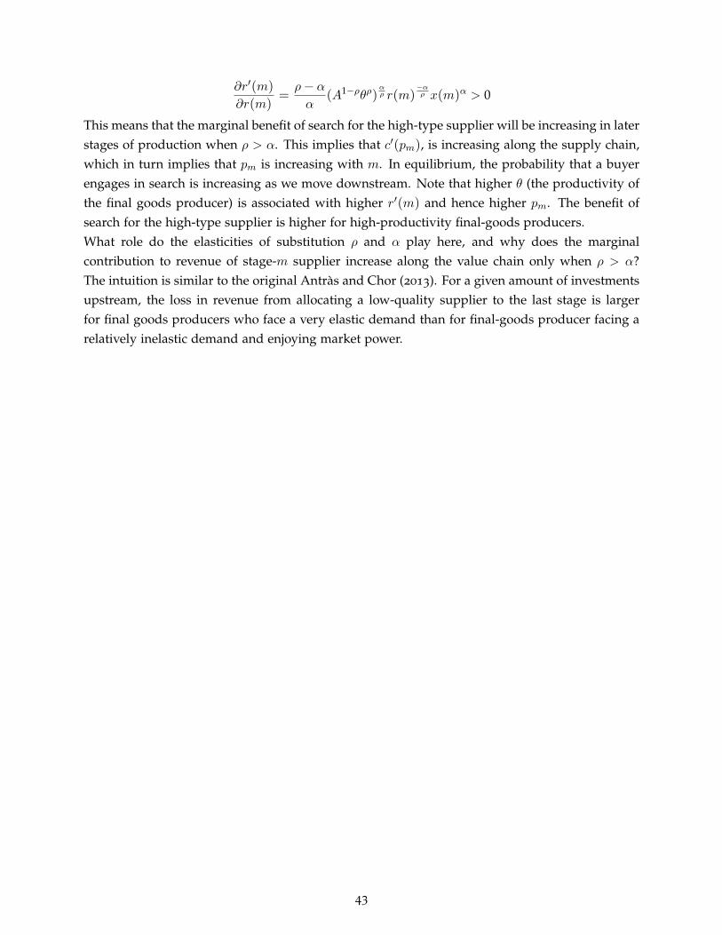
∂r′(m)

∂r(m)=ρ− αα

(A1−ρθρ)αρ r(m)

−αρ x(m)α > 0

This means that the marginal benefit of search for the high-type supplier will be increasing in laterstages of production when ρ > α. This implies that c′(pm), is increasing along the supply chain,which in turn implies that pm is increasing with m. In equilibrium, the probability that a buyerengages in search is increasing as we move downstream. Note that higher θ (the productivity ofthe final goods producer) is associated with higher r′(m) and hence higher pm. The benefit ofsearch for the high-type supplier is higher for high-productivity final-goods producers.What role do the elasticities of substitution ρ and α play here, and why does the marginalcontribution to revenue of stage-m supplier increase along the value chain only when ρ > α?The intuition is similar to the original Antràs and Chor (2013). For a given amount of investmentsupstream, the loss in revenue from allocating a low-quality supplier to the last stage is largerfor final goods producers who face a very elastic demand than for final-goods producer facing arelatively inelastic demand and enjoying market power.

43

References

Antràs, Pol and Davin Chor, “Organizing the Global Value Chain,” Econometrica, 2013, 81 (6),2127–2204.

, Daron Acemoglu, and Elhanan Helpman, “Contracts and Technology Adoption,” AmericanEconomics Review, 2007, 97 (3), 916–943.

, Davin Chor, Thibault Fally, and Russell Hillberry, “Measuring the Upstreamness of Produc-tion and Trade Flows,” American Economic Review Papers and Proceedings, 2012, 102 (3), 412–416.

Beil, Damian, “Supplier Selection,” in “Wiley Encyclopedia of Operations Research and Manage-ment Science” 2010.

Bernard, Andrew, Andreas Moxnes, and Karen Helene Ulltveit-Moe, “Two-Sided Heterogenityin Trade,” 2013. Mimeo, Dartmouth University.

, Bradford Jensen, Stephen Redding, and Peter Schott, “Importers, exporters, and multina-tionals: A Portrait of Firms in the U.S. that Trade Goods,” in Timothy Dunne, Bradford Jensen,and Mark Roberts, eds., Producer Dynamics: New Evidence from Micro Data, University of ChicagoPress, 2009.

, , , and , “Wholesalers and Retailers in US Trade,” American Economic Review, 2010, 100(2), 408–413.

, , , and , “The Empirics of Firm Heterogeneity and International Trade,” Annual Reviewof Economics, 2012, 4, 283–313.

Blum, Bernardo, Sebastian Claro, and Ignatius Horstmann, “Intermediation and the Nature ofTrade Costs: Theory and Evidence,” 2009. Mimeo, University of Toronto.

, , and , “Facts and Figure on Intermediated Trade,” American Economics Review Papers andProceedings, 2012, 100 (2), 419–423.

Broda, Christian and David Weinstein, “Globalization and the Gains from Variety,” QuarterlyJournal of Economics, 2006, 121 (2), 541–585.

Carballo, Jeronimo, Gianmarco Ottaviano, and Christian Volpe Martincus, “The buyer marginsof firms’ exports,” 2013. CEPR Discussion Paper 9584.

Costinot, Arnaud, John Vogel, and Su Wang, “An Elementary Theory of Global Supply Chains,”Review of Economic Studies, 2013, 80, 109–144.

Eaton, Jonathan, Marcela Eslava, David Jinkins, C.J. Krizan, Maurice Kugler, and James Ty-bout, “A search and learning model of export dynamics,” 2012. Mimeo, Penn State University.

Egan, Mary Lou and Asoka Mody, “Buyer-Supplier Links in Export Development,” WorldDevelopment, 1992, 3 (20), 321–334.

Garicano, Luis, “Hierarchies and the Organization of Knowledge in Production,” Journal ofPolitical Economy, 2000, 108 (5), 874–903.

Haltiwanger, John, Ron S. Jarmin, and Javier Miranda, “Who Creates Jobs? Small versus Largeversus Young,” Review of Economics and Statistics, 2013, 95 (2), 347–361.

Jarmin, Ron and Javier Miranda, “The Longitudinal Business Database,” 2002. Center forEconomic Studies, U.S.Census Bureau.

44

Kamal, Fariha and Asha Sundaram, “Buyer-Seller Relationships in International Trade: Do YourNeighbors Matter,” 2012. Mimeo, Center for Economics Studies, U.S. Census Bureau.

and C.J. Krizan, “Decomposing Aggregate Trade Flows: New Evidence from U.S. Traders,”2013. Working paper, Center for Economics Studies, U.S. Census Bureau.

Khandelwal, Amit, “The Long and Short (of) Quality Ladders,” Review of Economics Studies, 2010,77 (4), 1450–1476.

Kremer, Michael, “The O-Ring Theory of Economic Development,” Quarterly Journal of Economics,1993, 108 (3), 551–575.

Kugler, Maurice and Eric Verhoogen, “Prices, Plant Size and Product Quality,” Review of EconomicStudies, January 2012, 79 (1), 307–339.

Loecker, Jan De and Penny Goldberg, “Firm Performance in a Global Market,” Annual Review ofEconomics, 2014, 6 (xx), xx.

Maggi, Giovanni and Gene Grossman, “Diversity and Trade,” American Economics Review, 2000,90 (5), 1255–1275.

Manova, Kalina and Zhiwei Zhang, “Export Prices Across Firms and Destinations,” QuarterlyJournal of Economics, 2012, 127, 379–436.

Melitz, Marc, “The Impact of Trade on Intra-Industry Reallocations and Aggregate IndustryProductivity,” Econometrica, 2003, 71 (2), 1695–1725.

and Stephen Redding, “Heterogenous Firms and Trade,” in Gita Gopinath, Elhanan Helpman,and Kenneth Rogoff, eds., Handbook of International Economics, North Holland, 2014, Forthcom-ing.

Milgrom, Paul and Jon Roberts, “The Economics of Modern Manufacturing: Technology, Strat-egy, and Organization,” The American Economic Review, 1990, 80 (3), 511–528.

Pierce, Justin and Peter Schott, “A Concordance Between U.S. Harmonized System Codes andSIC/NAICS Product Classes and Industries,” Journal of Economic and Social Measurement, 2012,37 (1-2), 61–96.

Rauch, James, “Networks Versus Markets in International Trade,” Journal of International Eco-nomics, 1999, June, 1695–1725.

Sattinger, Michael, “Comparative Advantage and the Distribution of Earnings and Abilities,”Econometrica, 1975, XLIII (3), 455–468.

Sobel, Joel, “How to Count to One Thousand,” Economic Journal, 1992, 102 (3), 1–8.

Verhoogen, Eric, “Trade, Quality Upgrading and Wage Inequality in the Mexican ManufacturingSector,” Quarterly Journal of Economics, 2008, 123 (2), 489–530.

45