firm learning and growth - welcome | department of...
TRANSCRIPT

Firm Learning and Growth ∗
Costas Arkolakis Theodore Papageorgiou Olga A. Timoshenko †
Yale University and NBER McGill University George Washington University
March 24, 2017
Abstract
We study the implications of introducing learning (Jovanovic, 1982) in a standard
monopolistically competitive environment with firm productivity heterogeneity. Our
setup predicts that firm growth rates decrease with age, holding size constant, and
decrease with size, holding age constant, a fact that models focusing on idiosyncratic
productivity shocks have difficulty matching. We characterize the planner’s problem
and show that relative quantities between any two firms are the same in both planner’s
allocation and the decentralized economy. As a result, any inefficiency is driven by
a discrepancy in the firm entry and exit thresholds. We calibrate the model using
Colombian plant-level data and demonstrate how policies directly affecting firm entry
and exit can be welfare enhancing. In particular, age-dependent subsidies allow young
firms to avoid early exit and thus benefit consumers through access to a larger number
of varieties.
∗We are grateful to Manolis Galenianos, Illenin Kondo, Logan Lewis, Ryan Monarch, Giuseppe Moscarini,Emanuel Ornelas, Andres Rodriguez-Clare, Kim Ruhl, Erick Sager, James Tybout as well as various seminarparticipants. We also indebted to Shiva Kumar Venkatraman for outstanding research assistance. This researchis supported by NSF grant SES-0921673. This work was supported in part by the facilities and staff of the YaleUniversity Faculty of Arts and Sciences High Performance Computing Center and the George Washington UniversityColonial One High Performance Computing Initiative. All remaining errors are ours.†Contact: Arkolakis: [email protected], Papageorgiou: [email protected], Timoshenko:
1

1 Introduction
Policies intended to stimulate growth often provide subsidies for startups and young firms.1 Such
policies are poorly understood in workhorse models of firm dynamics where the determinant of
all firm decisions is size, not age, such as as Hopenhayn (1992), Klette and Kortum (2004), or
Luttmer (2007). To conduct such analysis we develop a quantitative learning model introducing
the Jovanovic (1982) firm learning setup into a monopolistically competitive economy.
In our model firms enter the market small and are uncertain about the demand their product
faces. Over time, as firms observe sales realizations, they may grow large if they have a very
successful product or, if not, they shrink and may eventually exit the market. More specifically,
the demand for a firm’s product is uncertain and demand realizations in each period are determined
by an unobserved idiosyncratic firm demand component, namely the firm’s product appeal in a
market plus a noise component. A firm that experiences higher demand than initially expected,
revises upward its belief, expands production and grows in size. A firm that experiences lower
demand than expected cuts back on production, and may even find it optimal to exit the market.
Using this basic Bayesian learning mechanism, our setup is able to replicate the observed higher
growth rate experienced by younger firms, even conditional on their size. First, younger firms face
large uncertainty about their product appeal, they revise their beliefs relatively more, compared
to firms that are older and better informed. In equilibrium, they are expected to grow faster
compared to older firms, even conditional on a firm’s size. Second, the endogenous selection of
firms strengthens the above result: Since younger firms face greater uncertainty, they are much
more likely to exit the market if they face a low demand realization. This selection implies that
the measured growth rate of surviving young firms is even higher than the respective growth rate
of older firms. While some early work by Evans (1987a) and Dunne et al. (1989) has suggested
that age might be an important determinant of growth, theoretical work has long ignored the role
of age in firm growth. A recent wave of research, led by Haltiwanger et al. (2013), has returned
the focus of empirical work on age, revealing its important role for firm growth.
To evaluate the significance of the learning mechanism for policy we characterize the planner’s
problem in this economy and show that relative quantities between any two firms are the same in
both the planner’s allocation and the market economy. Moreover, if the market economy’s entry
1See for instance the recommendations of Commision (2010) and the analysis and recommendations in chapter5 in the OECD (2013) report.
1

and exit thresholds coincide with those of the planner, perhaps as a result of a policy, then the
firms’ quantity decisions are efficient. This suggests that any inefficiency is driven by a discrepancy
in the firm entry and exit thresholds. This insight guides our search for optimal policies when we
perform welfare analysis in our calibrated economy.
To investigate the quantitative implications of our setup, we calibrate the model to match
moments from a panel of Colombian plant-level data, assuming that in our model each firm owns
a unique plant. Guided by our theoretical results, we identify the importance of learning by
targeting the impact of age on growth rates, conditional on size. In addition, the model correctly
predicts moments that are not targeted in the calibration, such as the annual survival rate and
the impact of size on growth rates, conditional on age. Furthermore, the model also matches the
non-linearity in the dependence of growth rates on age, conditional on size, as well as the decline
in the dispersion of firm growth rates as firm age.
Armed with the calibrated model, we explore policies that can potentially improve welfare.
Given our theoretical insights, we consider subsidies and taxes to the fixed cost of production:
these policies that directly impact firm entry and exit thresholds, while leaving relative quantities
unchanged. We consider a flexible subsidy schedule whereby the amount of the subsidy transfer
depends on a firm’s age, which can be easily observed and verified by a policymaker. The subsidies
we consider are financed through lump-sum taxation. Our results suggest that the optimal subsidy
is very high for young firms and can reach 50% for entrants and falls to 15% by age 5. Welfare
increases by 0.48% compared to the baseline economy. Furthermore, we consider the transition
dynamics from the implementation of the subsidy policy. We find that welfare declines initially
and increases thereafter. The discounted value of the policy remains positive, albeit considerably
smaller.
Our work follows the line of research that studies the impact of government subsidies on growth.
Acemoglu et al. (2013) extend the Klette and Kortum (2004) model to examine the optimal level
of subsidies to innovating firms, whereas Atkeson and Burstein (2010) study the impact of policy
on innovation and aggregate output in a wider class of models. Itskhoki and Moll (2015) study
policy in a growth setup with financial frictions. Unlike these papers, we do not consider a setup
with aggregate growth but instead a setup with firm dynamics in a stationary steady state. In our
context, some government policies may be welfare improving because of the interaction of learning
and monopolistic competition with love for variety. There are two key mechanisms through which
2

this interaction affects efficiency. First, in our setup with demand uncertainty, equilibrium entry
is lower than the efficient level. Second, by introducing a subsidy, some firms that would have
otherwise exited the market, receive additional signals, learn that in fact their underlying demand
is higher than they originally thought and grow large.
Moreover, our paper contributes to a new, but growing literature on the quantitative implica-
tions of learning on firm growth. Eaton et al. (2012) consider a model where firms actively learn
their product appeal by forming new matches with buyers. Abbring and Campbell (2003) also
develop a structural model of firm learning, which they estimate with data on Texan bars. Both
these frameworks are much richer in the specification of the learning mechanism, but they use a
partial equilibrium model and as such, they cannot be used for macro policy evaluation, a key focus
of our analysis. Ruhl and Willis (2014) modify a standard model with idiosyncratic productivity
shocks by specifying a foreign demand function that increases with firm age and Albornoz et al.
(2012) consider a model where a firm is uncertain about its demand and uncertainty is resolved
by incurring a fixed cost. David et al. (2016) consider the impact of imperfect information at the
firm level on input decisions and the extent to which imperfect information can lead to resource
misallocation. Their results suggest that imperfect information can result in sizeable productivity
losses. Finally, closer to our approach, Timoshenko (2015) develops a general equilibrium model
of learning in the context of multi-product firms and shows that such a framework can predict well
the age dependence of product switching among exporters.
Models that focus on idiosyncratic productivity shocks (Hopenhayn (1992), Luttmer (2007),
Arkolakis (2015)) have difficulty explaining the dependence of growth rates on age, conditional
on size.2 The reason for this failure is that growth is based on an underlying Markov process.
This assumption implies that all firms of the same size have the same growth profile, which is
independent of their age.3 Financial constraints together with idiosyncratic productivity shocks,
as in Cooley and Quadrini (2001), can explain age dependence (even conditional on size) if the entry
2Hopenhayn (1992) notes that “since size is a sufficient statistic for [productivity], age has no extra predictiverole” (page 1141).
3A similar reasoning applies to the Klette and Kortum (2004) approach. However, even if the productivity processis not a simple Markov process, but depends on a finite number of past realizations as well, the two approaches givedistinct predictions regarding the variance of sales as a function of age. The learning explanation proposed hereimplies that the variance of sales declines with age, as large firms become better informed regarding the demandthey face. However, productivity models have no such implication. In general, in a learning model, the dependenceof firm actions on past realizations does not erode away as the firm ages. This implication is used in Ericson andPakes (1998) to distinguish learning from a model of productivity shocks, in which the state dependence has ergodiccharacteristics.
3
of new firms is at high productivity levels.4 D’Erasmo (2011) and Clementi and Palazzo (2013)
show that adding convex and non-convex adjustment costs to Hopenhayn (1992) can generate age-
dependent growth. Adjustment costs imply that there is no longer a one-to-one mapping between
productivity and capital stock. As a result, firms of the same size can have different growth
rates which depend on both productivity and the capital stock. In equilibrium younger firms are
more productive, but have less capital, so by controlling for age in addition to size, one effectively
controls for both productivity and the underlying level of the capital stock. Our approach does
not require idiosyncratic productivity shocks to generate age dependence.5
The rest of the paper is organized as follows: Section 2 introduces our framework and considers
its both positive, as well as normative predictions. Section 3 contains the empirical section where
we use a panel of Colombian plant-level data to investigate data patterns that are consistent with
learning, calibrate our model and search for optimal policies. Section 4 concludes.
2 The Model
This section describes a model which introduces a demand-learning mechanism into a standard mo-
nopolistically competitive environment with firm productivity heterogeneity. The learning mech-
anism is similar to that of Jovanovic (1982) and firms must learn about their unobserved demand
level which is subject to transient preference shocks.
2.1 Environment
Time is discrete and denoted by t. The economy is populated by a continuum of consumers of
mass L. Each consumer derives utility from the consumption of a composite good, Ct, according
4In a multi-market setup, however, one can distinguish between our setup and the models of Jovanovic (1982)and Cooley and Quadrini (2001). Since a firm can have different demand realizations across markets, our frameworkis consistent with differential behavior of the same firm across the various markets in which it operates. For instance,it is possible that a firm expands production in a given market, while choosing to exit another one. If the financialconstraints are important or if the firm is learning about its underlying cost structure, then its behavior is restrictedto be the same across markets. Furthermore, the evidence in Eaton et al. (2008), Albornoz et al. (2012), Fitzgeraldet al. (2016) suggest that the age of a firm in a market is inversely related to firm growth and probability of exit inthat market, as implied by our model.
5It is worth pointing out that while age dependence always takes place in a Jovanovic learning model the sign ofthat dependence and its quantitative magnitude depend on the functional form assumptions. In our context withCES demand and monopolistic competition we find that growth rates always decline with firm age, conditional onsize, as discussed earlier.
4
to the utility function
U =+∞∑t=0
βt ln (Ct) ,
where β is the discount factor. The composite good consists of the consumption of a contin-
uum of differentiated varieties ct(ω), aggregated using a constant elasticity of substitution (CES)
aggregator with elasticity of substitution σ > 1
Ct =
(∫ω∈Ωt
(eat(ω)
) 1σ ct (ω)
σ−1σ dω
) σσ−1
, (1)
where Ωt is the continuum of differentiated varieties available at time t; at (ω) is the demand shock
at time t for variety ω ∈ Ωt. Consumers are endowed with one unit of labor that they inelastically
supply to the market to receives a wage, wt, in return. They also own an equal share of domestic
firms.
Each variety is supplied by a monopolistically competitive firm and the realization of the
demand variable at (ω) for each good is determined by a time invariant component, θ(ω), and a
shock, εt(ω), and is given every period by
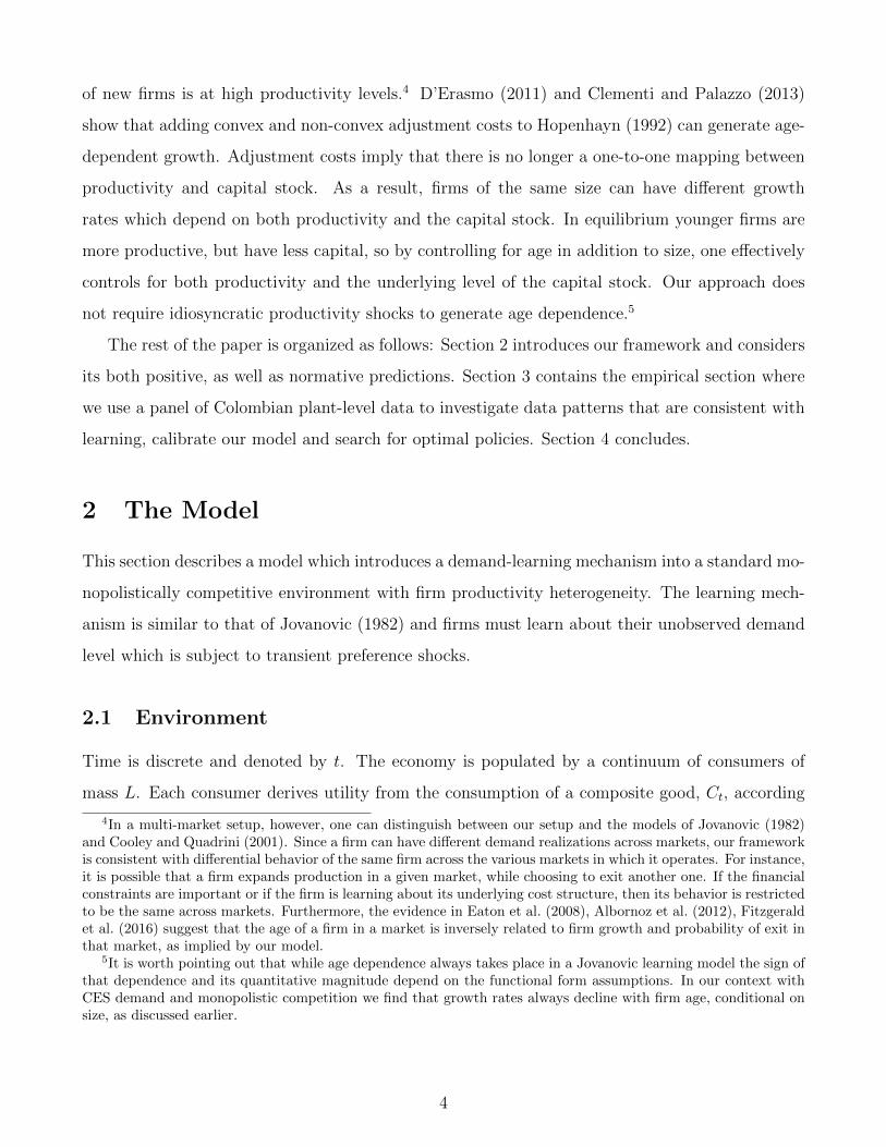
at (ω) = θ (ω) + εt (ω) , εt (ω) ∼ N(0, σ2
ε
)i.i.d.
The time-invariant demand parameter, θ (ω), can be interpreted as the true underlying demand
for a product, its product appeal, and it is unobserved by the firm. This is subject to transient
preference shocks, εt(ω), which are independent over time and across products.
Following Chaney (2008), we assume that every period there is an exogenous mass of potential
entrants J . Entrants draw their unobserved demand parameter, θ (ω), from a normal distribution
with mean θ and variance σ2θ. There is no sunk cost of entry. These firms maximize the expected
present discounted value of profits and have the same discount factor as consumers, β. Firms exit
the market either exogenously with probability δ or endogenously if the sum of their discounted
expected profits is less than zero. If the firm stays in the market, it decides the quantity to be
produced, qt (ω). Output is linear in labor, lt (ω), which is the only factor of production, and there
is a fixed cost of production, f , measured in the units of labor. Firms are heterogeneous in their
productivity level, ez(ω), which is drawn upon entry and is time-invariant (in Appendix G we relax
this assumption and allow productivity to change over time). Unlike the demand parameter, θ (ω),
5

each firm’s productivity level is observed by the firms. Realized firm profits after accounting for
variable and fixed costs are πt (ω) =(pt (ω)− w/ez(ω)
)qt (ω)− wf .
The sequence of actions is the following: At the beginning of each period, each incumbent
firm decides whether to stay in the market and what quantity to produce or to endogenously exit.
Next, potential entrants draw their productivity, ez(ω), and their (unobserved) demand parameter,
θ (ω), and decide whether to sell or exit. Those that decide to sell pay the fixed cost of production.
Subsequently, the firm decides the quantity produced, production takes place and the firm delivers
the good to the market. After all firms have delivered their quantity to the market, the demand
shock, at (ω), is realized and the price of each good, pt (ω), adjusts so that the good’s market clears.
After the market has cleared, the firm observes the realized price, infers the underlying demand
realization and updates its belief for its product appeal. Finally, firms exit the market exogenously
with probability δ.
2.2 Consumer Demand
Each consumer chooses the consumption levels, ct (ω), to minimize the cost of acquiring Ct taking
into account the prices of varieties, pt (ω), as well as his income. The resulting demand equation
for each variety is given by
qt (ω) = eat(ω) (pt (ω))−σ
P 1−σt
Yt, (2)
where Yt is the aggregate spending level and is given by Yt = wtL+ Πt, while Πt is total profits of
firms which are redistributed to consumers via a lump-sum payment,
Πt =
∫ω∈Ωt
πt (ω) dω.
Pt is the aggregate price index associated with the consumption of the composite good Ct and is
given by
P 1−σt =
∫ω∈Ωt
eat(ω) (pt (ω))1−σ dω. (3)
To economize on notation, in what follows we drop the variety index ω.
For the rest of the model description and for most of the exercise we focus on a stationary
equilibrium where the aggregate expenditure, Yt, the price index Pt, and the wage rate, wt, are
constant in the equilibrium. Hence, we suppress the time notation on the aggregate variables.
6

2.3 Firm Optimization
Each firm has to make two decisions every period: whether to stay in a market or exit and how
much to produce, if it chooses to stay. When the firm decides whether to produce or exit, it takes
into account not only that period’s profits, but also the value of learning by observing demand
realizations. We assume that at the start of each period a firm makes a quantity decision before
observing the current demand shock. Once the quantities are set the goods market clears and the
firm observes the market clearing price and, using the inverse demand function (2), infers the size
of the demand shock. When deciding how much to produce however, learning considerations are
not a factor, since the demand realization is independent of how much the firm produces. Therefore
its quantity choice is a static one.6 We begin by analyzing the beliefs formed by the firm, continue
with the static quantity decision, and then consider the entry and exit decision.
Belief Updating
Denote by a the mean of the observed shocks and by n the number of the observed shocks.
Since the firm receives one shock per period, n also corresponds to the firm’s age. Using Bayes’
rule, the firm updates its beliefs regarding θ: the posterior belief of a firm that has observed n
signals with mean a, is given by a normal distribution with mean
µn =σ2ε
σ2ε + nσ2
θ
θ +σ2θ
σ2ε + nσ2
θ
na , (4)
and variance
ν2n =
σ2θσ
2ε
σ2ε + nσ2
θ
.
Thus, the belief of the firm regarding the realization of its demand shock, at, followsN (µn, ν2n + σ2
ε).
An entrant knows the distribution from which the demand parameter is drawn, and that distribu-
tion serves as the prior. Notice that in the long run, upon observing infinitely many signals, the pos-
terior belief converges to a degenerate distribution centered at a and limn→∞ a = limn→∞
∑ni=0 ain
=
E(at) = θ. Thus, in the long run, firms learn their product appeal level, while in the short run
their knowledge can be summarized by the two state variables: the number of observed shocks n,
and the mean of the observed shocks a.
Quantity Decision
6See Bergemann and Valimaki (2000) and Eaton et al. (2012) for models of active learning and experimentation.
7

The static per-period profit maximization problem is given by
maxqtEat|n,a [pt (at) qt]− w
qtez− wf, (5)
subject to the consumer inverse demand
pt (at; qt) =
(eatY
qt
) 1σ
Pσ−1σ . (6)
Substituting the inverse demand constraint (6) into the static maximization problem (5) and
taking the first order conditions leads to the optimal quantity choice given by
qt (z, a, n) =
(σ − 1
σ
)σ (b(a, n)ez
w
)σY
P 1−σ , (7)
where we define
b(a, n) ≡ Eat|a,n(eatσ ) = exp
µnσ
+1
2
(ν2n + σ2
ε
σ2
), (8)
i.e. the firm’s belief regarding (eat). Notice from equation (7) that firms which are more productive
(have higher z) and firms which have higher beliefs regarding θ (have higher a and hence higher
b) sell more.
Substituting the firm’s quantity choice, equation (7), into the consumer inverse demand, equa-
tion (6), gives the market clearing price
pt (at, z, a, n) =σ
σ − 1
w
ezeatσ
b(a, n). (9)
The price depends on the firm’s productivity, z and belief, b, as well as the realization of the
demand shock, at. Taking expectation with respect to at, the expected market clearing price is
given by
Ept =σ
σ − 1
w
ez.
Thus, in expectation, price is a constant mark-up over marginal cost.
Substituting the optimal quantity and price into equation (5), the expected per-period firm
8

profits are given by
Eπ (z, a, n) =(σ − 1)σ−1
σσb(a, n)σ
(ez
w
)σ−1Y
P 1−σ − wf. (10)
Notice that, since σ > 1, profits are a convex function of firm beliefs.
Exit and Entry Decision
As discussed above, a firm decides whether to continue paying the fixed cost and stay in the
market or exit, taking the maximized expected profits, Eπ, as given. Thus, the value of a firm of
age n ≥ 0, with productivity z and observed shocks mean a, is given by
V (z, a, n) = maxEπ(z, a, n) + β(1− δ)Ea′|a,nV (z, a′, n+ 1), 0
, (11)
where the value of exit is normalized to zero. We assume that potential entrants pay the fixed
per-period cost and start to sell in the initial period if the value of entry is greater than zero,
otherwise exit immediately.
Since all the potential entrants draw their demand shock from the same distribution they start
with the same prior belief. From equation (8), the potential entrant’s belief is given by
b0 = exp
θ
σ+
1
2
(σ2θ + σ2
ε
σ2
). (12)
Notice that potential entrants do vary in terms of their productivity draw, ez. Thus, the entry
condition determines a productivity threshold value z, such that an entrant that draws productivity
z < z, exits immediately. The condition
V (z, θ, 0) = 0. (13)
pins down implicitly the productivity entry threshold z.
2.4 Stationary Equilibrium
To study the equilibrium we normalize the wage rate, w, to 1. Let M denote the equilibrium mass
of operating firms in every period and m(z, a, n) denote the mass of firms in state (z, a, n). Given
the entry and exit decisions of firms, the mass of firms evolves according the following transition
9

rule
m(z, a, n+ 1) =
∫ +∞
a∗(n,z)
(1− δ)m(z, ˆa, n)1√
υ2n + σ2
ε
φ
(a(n+ 1)− ˆan− µn
(ˆa)√
υ2n + σ2
ε
)dˆa. (14)
The mass of entrants is given by
m (z, 0, 0) =
J · g(z) for z > z
0 otherwise
,
where g(z) is the distribution from which entrants draw their productivity and a∗(n, z) is the firm
exit threshold rule.
The stationary equilibrium of the economy is described by the aggregate price index P , the
aggregate expenditure level Y , total profits of firms Π, the mass of operating firms M , the proba-
bility mass function m(z, a, n), the wage rate w, firms’ quantity choice q(z, a, n), firms’ entry and
exit decisions, z and a∗(n, z) consumers consumption choice c such that
1. Consumers are optimizing: given equilibrium values, c satisfies demand equation (2).
2. Firms are optimizing: given equilibrium values, q(z, a, n), z and a∗(n, z) solve the firm’s
optimization problem in equations (7), (13) and (11).
3. Goods market clears: Y = wL+ Π.
4. The labor market clears: L =∑+∞
n=0
∫ ∫q (z, a, n) /ezm(z, a, n)dzda+ fM .
5. The probability mass function m(z, a, n) delivers the aggregate mass of firms, M , i.e. M =∑+∞n=0
∫ ∫m(z, a, n)dzda.
6. The probability mass function m(z, a, n) satisfies the stationary flow condition (14).
2.5 Positive Implications
This section presents two key positive predictions of introducing learning into a heterogeneous-
firms model: the expected growth rate of a firm declines with age, conditional on size, and it
also declines with size, conditional on age. We summarize the two results in Propositions 1 and 2
below.
10

Proposition 1. The expected growth rate of a firm declines in age, conditional on size.
Proof. See Appendix A.
In our model, the learning mechanism lies at the heart of the conditional age dependence of
growth rates stated in Proposition 1. Let the expected growth rate of a firm be given by E (qt+1/qt).
As shown in Appendix A, using the expression for the optimal quantity choice in equation (7) and
in the absence of endogenous exit, the expected growth rate is given by
E
(qt+1
qt
)= exp
(λ2σ2
ε (σ − 1)
2σ (1 + nλ) (1 + (n+ 1)λ)
), (15)
where λ = σ2θ/σ
2ε . Notice that a firm’s age n only appears in the denominator. Hence, for a given
productivity level z and conditional on the firm’s initial size, qt, the expected growth rate of young
firms is higher than the growth rate of older firms. This result depends crucially on σ > 1.
To further understand the intuition of the above result, notice from equation (7) that a firm’s
optimal choice of output is a convex function of beliefs, b, through the term bσ. The convexity of
the output choice function implies that the increases in output when b increases are larger than the
declines in output when b falls by the same amount. Since young firms face more uncertainty than
older firms, their beliefs are expected to change by a larger amount. Higher volatility of beliefs, b,
combined with the convexity of the output choice function in b, leads to a high expected growth
rate. On the contrary, beliefs of older firms are less volatile leading to a lower expected growth
rate. Note that with no endogenous exit, the level of firm size, q, has no impact on the expected
growth rate, since it has no impact on the volatility of beliefs. Therefore Proposition 1 holds even
conditional on firm size.
In addition, if we allow for endogenous exit, the observed growth rate is even larger for young
firms near the exit threshold than what is implied by equation (15). The reason is that the firms
that observe low sales realizations may choose to exit the market, rather than stay in and record
low or negative growth rates. This mechanism is behind the next result.
Proposition 2. The expected growth rate of a firm declines in size, conditional on age.
Proof. See Appendix A.
The basic intuition behind Proposition 2 is the following: First, consider equation (15) which
computes the expected growth rate of a firm in the absence of selection. Notice that, conditional on
11

0 5 10 15 20 25 30−4
−3
−2
−1
0
The Number of the Observed Demand Shocks
The
Mea
n of
the
Obs
erve
d D
eman
d S
hock
s
A
B
Figure 1: Demand Shock and Exit Thresholds. Source: Author’s calculations on model simulations.
age, n, all firms are expected to grow at the same rate. More specifically, the expected growth rate
is independent of a firm’s productivity, z, and of the expected number of the observed demand
shocks, a. Thus, without controlling for selection, the growth rate is independent of a firm’s
initial size, qt. Put differently, the conditional size dependence of growth rates arises solely due to
endogenous exit as in Hopenhayn (1992).
The size dependence, hence, can only arise due to the endogenous selection. This is demon-
strated in Figure 1 which depicts, for a given productivity level z, the exit thresholds a∗(n, z) as
a function of firm age, n. The depicted exits thresholds are solutions to a firm’s entry and exit
problem described in Section 2.3. A firm of age n continues to sell if a > a∗(n, z) and exits other-
wise. The exit threshold a∗(n, z) increases with n because as firms become more confident about
their latent demand, i.e. n increases, the informational value of additional observations declines
and firms remain in the market only if their (expected) profit flow is sufficiently high.
To gain intuition regarding Proposition 2, consider two firms, Firm A and Firm B, that have
the same age, n, and productivity, z, but vary in terms of their mean of the observed demand
shocks, a. Since Firm A’s a is higher, its size, qt, is also larger compared to Firm B. Figure 1
plots the firm exit threshold as a function of a and n. Notice how Firm A is further away from
the exit threshold compared to Firm B. Since Firm B is located much closer to the exit threshold,
the only way it can survive in the next period is only if it grows by a sufficiently high amount.
Hence, conditional on survival, Firm B is expected to grow faster compared to Firm A. As shown
in Appendix A, the above result holds more generally in the case where the two firms have the
same size, but different productivity levels, z.
The above two propositions provide a theoretical foundation for the empirical findings of Evans
12

(1987b) and Haltiwanger et al. (2013). This literature establishes age as an additional determinant
of firm growth, other than size. More precisely they find that a regression of firm growth rates on
firm size and age yields negative and significant coefficients on both variables, which is consistent
with Propositions 1 and 2.7
It is worth pointing out that various authors have suggested models based on idiosyncratic
productivity shocks combined with additional mechanisms in order to explain age dependence,
conditional on size. Cooley and Quadrini (2001) generate conditional age dependence of growth
rates assuming a persistent productivity process in a model with financial frictions. In their
framework firms are heterogeneous in their productivity and new entrants start off with a high
level of productivity. The interaction of that assumption with financial frictions imply that more
productive young firms are able to borrow more than less productive older ones. Hence, the young
grow faster, even conditional on size. Models that focus on idiosyncratic productivity shocks
(Hopenhayn (1992), Luttmer (2007), Arkolakis (2015)) have difficulty explaining the dependence
of growth rates on age, conditional on size. The reason for this failure is that growth is based
on an underlying Markov process. In those setups two firms with the same size will have the
same expected growth rate. Finally, D’Erasmo (2011) and Clementi and Palazzo (2013) study
a Hopenhayn (1992) model with convex and non-convex adjustment costs. The introduction of
adjustment costs implies that young firms are below their target capital level and, as a result, are
more likely to expand their capital and grow, even conditional on their initial size.8
In our framework all that is required to generate conditional age dependence is a learning
mechanism. While in our model we also assume heterogeneity in productivities, as can be seen
from equation (15), age dependence holds for any productivity level. In Appendix G we calibrate
a model with productivity evolution and find that productivity shocks account for less than ten
percent of the conditional age dependence.
2.6 Normative Implications
We now turn to examine the normative predictions of the model. We first set up the planner’s
problem, characterize the planner’s allocation and compare the solution to the stationary market
equilibrium. The results of this section guide the empirical investigation of different policies in
7See also Eaton et al. (2012), Arkolakis (2015) for related evidence on exporters.8See also Castro et al. (2004).
13

Section 3.4.
We focus on a stationary economy and consider the problem of a planner who faces the same
information constraints as the agents of our economy and maximizes the steady state utility of the
representative consumer:9
maxI(z,a,n),N(z),qP (z,a,n),qP (z,a,n)
lnC∗ (16)
subject to (a) the definition of C∗, given by (1), (b) the labor market clearing condition as stated
in condition 4 of the stationary equilibrium definition, (c) the stationary flow conditions for the
mass of firms, equation (14) discussed in Section 2.4, where I(z, a, n) ∈ 0, 1 is the market
participation decision chosen by the planner for the incumbents of type (z, a, n), N(z) ∈ 0, 1
is the entry decision for entrants of type z, qP (z, a, n) is the quantity chosen by the planner for
incumbents of type (z, a, n) and qPe (z) is the quantity chosen for entrants of type z.
Proposition 3. The stationary planner’s quantity decisions for all the active firms in the economy
are given by
qP (z, a, n) =(ezb(a, n))σ (L− fM)
A, for n ≥ 1 (17)
qPe (z) =(ezb0)σ (L− fM)
A(18)
where A is defined in equation (38) of Appendix B.
Proof. See Appendix B.
Comparing the planner’s quantity choices, (17) and (18) with those of our baseline economy,
(7), it becomes apparent that they are the equal up to a multiplicative constant. This implies that
the relative quantities between any two firms are the same in both planner’s allocation and the
market economy. Corollary 4 below states that any stationary allocation that has the same entry
and exit thresholds as the planner, is efficient.
Corollary 4. If there exist lump-sum transfers to firms such that the resulting entry and exit
thresholds coincide with those of the planner, I(z, a, n) and N(z), then the quantity decisions also
coincide with those chosen by the planner.
Proof. See Appendix B.
9We explicitly consider stationary allocations for the planner excluding the possibility of optimal policies thatare not stationary.
14

In Appendix B we characterize the planner’s exit thresholds for every firm type. Even though
firms entry and exit thresholds do not admit a closed form expression in either the planner’s
problem or the general equilibrium, Corollary 4 enables us to conclude that any inefficiency must
be driven by a discrepancy in entry and exit. We next discuss why such a discrepancy might
occur and then, in Section 3.4, guided by the above results, examine the welfare properties of our
calibrated economy.
Any change in the economy’s the entry and exit thresholds has a direct effect in the number of
varieties available to the representative consumer. For concreteness, consider a decrease in the exit
threshold for some types, (z, a, n), which leads to more varieties being available in equilibrium. An
increase in the number of varieties has a direct effect on the equilibrium welfare as measured by real
consumption C. In particular, from equation (1), an increase in Ω increases the real consumption,
holding all else constant. Grossman and Helpman (1991) refer to this as the consumer-surplus
effect. An increase in the number of varieties at the same time however may reduce welfare because
of what Grossman and Helpman (1991) refer to as the profit-destruction effect. In particular, more
varieties implies that a greater amount of labor is used to cover firm fixed costs. As a result less
labor is used in the production of the final good, yielding less disposable income available to
consumers and reducing per variety consumption, c (ω). Indeed, as discussed in Appendix B, the
planner’s optimal exit thresholds take into account how a slight decrease leads on one hand to more
varieties, on the other hand to more labor being used to cover fixed costs. In addition, there’s also
a third effect capturing dynamic considerations and how this decline in the threshold affects the
distribution of firms of all types in the stationary equilibrium.
In the competitive market, when a firm makes an entry/exit decision it does not internalize the
benefits to consumers of an additional variety, nor the adverse effects on the profits of incumbent
firms through the monopolistic distortion.10 These two effects exactly cancel out in the basic setup
with CES demand and, as a result, efficiency holds even in the presence of firm heterogeneity, as
pointed out by Dhingra and Morrow (2012). The introduction of demand uncertainty implies that,
when a firm is active, there is an option value from learning. The firm takes this option value
into account when deciding whether to enter or exit. Put differently, the presence of learning
alters firm’s entry and exit decisions compared to the static monopolistic competion model (Melitz
(2003)) and as a result our model of learning implies the possibility of an inefficiency, compared
10Again, see discussion in Grossman and Helpman (1991), page 82.
15

to competitive learning model of Jovanovic (1982).
In Section 3.4, using our calibrated model, we show that the market economy is constrained
inefficient and that policies that appropriately target firms’ entry and exit thresholds can lead to
welfare improvement.
3 Quantitative Results
In this section we explore the quantitative implications of our model. We first discuss the data,
calibrate the model and finally examine the magnitude of the potential welfare gains from a targeted
policy intervention.
3.1 Data Patterns Consistent with Learning
We begin by documenting some empirical regularities that are consistent with learning. We use
the Colombian plant-level data collected in the DANE survey (see Roberts (1996)). The data cover
all the manufacturing plants in Colombia with 10 or more employees for the period of 1983-1991.11
For our purposes this database is particularly informative since it reports some key variables of
interest: the real output of the plant and the age of the plant (i.e. the year of a plant’s start-up
which we use to infer the plant’s age). We denote sales as the real value of production reported
in the survey; the growth rate measures the growth in sales between two consecutive periods. We
consider plants with age up to 20 years. In Appendix C we discuss additional details of the data
and the construction of the data moments later used in the calibration.
A robust empirical regularity in our data is that conditional on size, young plants grow faster
(see first column of Table 3 in Section 3.3 below). A plant with twice the age has an average
growth approximately 3% less. As discussed in detail in Appendix D, the finding is also robust if
we allow for industry fixed effects, as well as other controls.12
11Earlier data from 1977 to 1982 cover all manufacturing plants in Colombia but the data on real production arenot as reliable for that time period. To avoid measurement bias caused by the change in the coverage we use onlythe latest part of the survey, 1983-1991.
12In Appendix D we also consider alternative explanation such as financial constraints and non-convex costsof adjustment for investment and show that the age dependence remains robust. For example, we augment ourempirical specifications to allow for additional variables that proxy for financial constraints and find that the agecoefficient remains large and statistically significant. In addition, we explore how the conditional age effect varieswith age by flexibly running the above specification using age dummies (see also Haltiwanger et al. (2013)). Theage effect is stronger for younger firms and is statistically indistinguishable from zero after age 5.
16

In subsection 3.3 below we also consider how the cross-sectional standard deviation of growth
rates changes with age. We find that it declines sharply with age consistent with model’s predictions
discussed below.
In the next subsection, we discuss how we use the conditional age dependence to calibrate our
model and assess its quantitative fit.
3.2 Calibration
For the calibration we assume that the data has been generated from the steady state of our
model and match theoretical moments to their empirical counterparts. We also treat a plant in
the data as a firm in the model. In addition, we assume that each potential entrant draws its
productivity ez from the a Pareto distribution with parameter ξ > 0. The computation of the
stationary equilibrium is briefly outlined in Appendix E.13
We first specify some of the parameters independently. In particular, we set the elasticity of
substitution across goods, σ, to 7.49 following Broda and Weinstein (2006). Similarly we set the
discount factor, β, to 0.9606, which implies a quarterly discount rate of 1%. Given this, we set δ
to 0.025 to generate an exit rate of 2.56% among the largest 5% of plants in the Colombian data,
where exit happens only exogenously.
The remaining parameters are jointly calibrated. To be precise, we calibrate the following
four parameters: the per period fixed cost, f , the standard deviation of demand shocks, σε, the
shape parameter of the distribution of the productivity draws, ξ, and the standard deviation of the
distribution of the unobserved demand parameters, σθ.14 In order to calibrate the parameters, we
use the following four moments: the mean of log sales; the sales-weighted growth rate of entrants;
the entrants’ share of sales; and, following the discussion above, the age coefficient in the regression
of firms growth rates on age and size.
Although a rigorous identification argument is not possible due to the complexity of the setup,
we give an informal argument of how each parameter is identified from the data. The per period
fixed cost, f , is pinned down by the mean log sales, since increasing the fixed cost leads less
productive firms to exit the market thereby increasing the mean sales. The shape of the distribution
of the initial productivity draws, ξ, is pinned down by entrants’ share of sales: A lower value for
13The simplex search method is used to search over the parameter space (ξ, f, σε, σθ). To compute the simulatedmoments, 40,000 firms are simulated.
14Note that θ in this setup is not separately identified from f , so we set θ = 0.
17

Parameter Value
ξ 13.09σε 1.46σθ 0.997f 253,181
Table 1: Parameter Values. Model Baseline Calibration.
Targeted Moments: Data Model
Mean of log-sales 14.99 14.99Share of sales from entrants 2.66% 2.66%
Sales-Weighted growth rate of entrants 23% 23%Age Coefficient -0.035 -0.035
Other Moments:Annual Survival Rate 91% 91%
Table 2: Data and Simulation Moments. Sources: DANE survey data (see text for details) andModel Baseline Calibration.
ξ, all else equal, leads to a higher initial productivity dispersion and therefore more entrants
starting off relatively large. Finally, the parameters related to the learning process, σε and σθ are
pinned down by the sales-weighted growth rate of entrants and the age coefficient. The calibrated
parameters for this baseline calibration are presented in Table 1 and the targeted moments are
presented in Table 2.
As shown in Table 2, the fit for all four moments is close to exact. In addition, Table 2 reports
the annual survival rate. This moment was not targeted in the calibration and, nevertheless, the
predicted coefficient is very close to the empirical one. Given that learning affects both the growth
and the exit behavior of firms, it’s reassuring that our model is able to match this moment as well.
3.3 Quantitative Fit
In this section we explore the quantitative implications of the calibrated model in terms of its
ability to generate unconditional and conditional growth results, as well as the decline in the
cross-sectional standard deviation of growth rates.
Figure 2 depicts the unconditional relationship between a firm’s growth and age (Panel A), and
a firm’s growth and size (Panel B) for the simulated and actual data. Observe from both panels
of Figure 2 that Colombian data resembles similar patterns as found in the empirical literature:
18
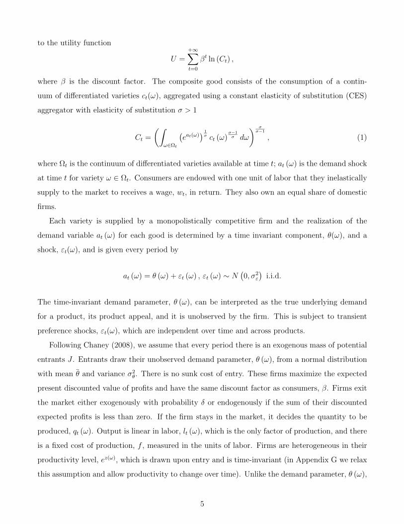
the growth rate declines in age and the growth rate declines in size.15
2 4 6 8 10−0.05
0
0.05
0.1
0.15
0.2
Age
Loga
rithm
of C
umul
ativ
eG
row
th R
ate,
Mea
n
Panel A
2 4 6 8 10−0.05
0
0.05
0.1
0.15
Sales Decile
Loga
rithm
of C
umul
ativ
eG
row
th R
ate,
Mea
n
Panel B
DataSimulations
DataSimulations
Figure 2: Growth Rates with Age and Size. Source: DANE survey data and authors’ calculationson model simulations.
The learning model is able to capture reasonably well both of these dependencies. As shown in
Panel A 2, our model can replicate the non-linear relationship between growth and age, as young
firms quickly learn their latent demand parameters.16 Further, as shown in Panel B of Figure 2,
the relationship between growth and size declines faster in the model compared to the data. This
is partially driven by large firms in the model exhibiting negative growth rates. In the model,
sales depend on price realizations, which, in turn, depend on realizations of the preference shocks.
Hence, an unusually large positive preference shock increases observed sales. However, since these
shocks are transitory, there is mean reversion, so the following period realized sales will be lower
on average yielding the negative growth rates observed in the figure.17
Moreover, the model is able to capture well the conditional size dependence of growth rates as
presented in Table 3. While the age coefficient was one of the targeted moments in the calibration,
the size coefficient was not and the model is able to match this moment well.
Next, we consider how quickly the conditional age dependence vanishes as plants grow older.
In order to flexibly measure the impact of age, we run our baseline conditional growth regression
using age dummies. Panel A of Figure 3 depicts the relation between a plant’s age and the
15See Evans (1987a,b), Dunne et al. (1989), D’Erasmo (2011) and also Eaton et al. (2008), Arkolakis (2015) andBastos et al. (2016) for exporters.
16In the simulated data, in contrast to the actual data, the growth rate gradually approaches zero as age rises.This is expected, since only source of firm growth in the model is learning. Once firms learn their true demandlevel, they experience no further growth
17Indeed, when the variance of the preference shock, σε, falls, the growth rate of large firms converges to zerofrom below.
19

Data ModelSales Growth Rate Sales Growth Rate
ln(sales) -0.022 -0.022(0.002)∗∗∗ (0.001)∗∗∗
ln(plant age) -0.035 -0.035(0.002)∗∗∗ (0.001)∗∗∗
constant 0.428 0.411(0.022)∗∗∗ (0.014)∗∗∗
R2 0.02 0.03Number of Observations 36,877 205,882
Table 3: Growth dependence on Age and Size in the Data and Model. Standard errors clusteredby plant. ∗∗∗ denotes significance at the 1% level. Source: DANE survey data (see text for details).
0 5 10 15 20Plant Age
-0.05
0
0.05
0.1
0.15
Age
Dum
my
Coe
ffici
ent
DataModel
0 5 10 15 20Plant Age
-0.1
-0.05
0
0.05
0.1
0.15
Cha
nge
in S
t Dev
of S
ales
Gro
wth
Rat
es DataModel
Figure 3: Panel A (left): Growth dependence by Age conditional on Size, Data vs Model. PanelB (right): Change in Cross-Sectional Standard Deviation of Sales Growth Rates by Age, Data vsModel. Source: DANE survey data and authors’ calculations on model simulations.
corresponding estimate of the age dummy in the conditional growth regression. The solid line
refers to the estimates from the data. As can be seen in Panel A of Figure 3, the conditional age
effect is highly non-linear. The dashed line replicates the results using the simulated data. The
figure demonstrates that the model is able to match the non-linear conditional age dependence of
growth rates quite well.
Finally, we examine the relationship between the cross-sectional standard deviation of the sales
growth rates and age. In our setup, as new information arrives, the change in the firm’s posterior
belief becomes smaller. This leads to a smaller change in the firm’s quantity decision from one
period to the next and implies that we should observe a lower standard deviation in growth rates as
firms grow older. Panel B of Figure 3 depicts the relationship between firm age and the standard
20

deviation of the growth rates for the data (solid line) and the model (dashed line). While our
calibrated model underpredicts the overall level of the cross-sectional standard deviation of sales
growth rates, it is able to match its decline with age.18
3.4 Implications for Welfare
Guided by the normative findings of Section 2.6, we explore policies that can potentially improve
welfare. More specifically, given the insight of Corollary 4, we focus on policies that affect firms’
entry and exit decisions and do not directly target the firms’ quantity decisions.
One straightforward way to implement welfare maximizing thresholds is by subsidizing or taxing
firms’ fixed costs and simultaneously imposing a lump-sum tax on the consumers. Denote by
τ(z, a, n) a fixed cost subsidy or tax applied to a firm of type (z, a, n). Hence, 0 < τ < 1 represents
a fixed cost subsidy whereby a firm pays τf portion of the fixed costs and the portion (1 − τ)f
is transferred (by the government) from consumers to each of the subsidized firms. In contrast,
τ > 1 represents a fixed cost tax whereby a firm pays a fixed cost in the amount of τf , and the
portion (τ − 1)f is transferred from each of the taxed firms to consumers.
With this set of instruments, the problem of the firm described in equation (11) becomes
V (z, a, n) = maxEπ(z, a, n)− (τ(z, a, n)− 1)f + β(1− δ)Ea′|a,nV (z, a′, n+ 1); 0. (19)
Notice that the fixed cost subsidy or tax rate τ does not affect the intensive margin decisions
of firms. The firm’s optimal quantity choice is included in the expected profit Eπ(z, a, n) and
is determined by the static per-period profit maximization problem described in (5). The policy
however does affect entry and exit choices of firms. For instance, any subsidy, τ(z, a, n), increases
total expected profits and hence reduces the incentive to exit, all else equal. As a result, the
corresponding exit thresholds declines. Summarizing, the proposed set of policies directly affects
a firm’s incentive to stay or exit and does not change the relative quantities of firms, consistent
with equations (17) and (18) of the planner’s problem.
Our empirical analysis focuses on fixed costs subsidies or taxes, τ(.) that depend on only a
firm’s age, n. While fixed cost subsidies or taxes can in theory depend on any of the firm’s state
18In our setup the predicted standard deviation of sales growth rates is 0.25 while in the data it is 0.41. Ourcalibration does not target any cross-sectional dispersion moments and our mechanism’s key implications focus onthe change of growth rate dispersion with age, rather than its level.
21

Age0 2 4 6 8 10
The
sha
re o
f fix
ed c
osts
paye
d by
a fi
rm
0.4
0.5
0.6
0.7
0.8
0.9
1
Figure 4: Optimal Subsidy Schedule. Authors’ calculations on model simulation.
variables, i.e. also its productivity, z, and its beliefs, b, we choose to focus only on age, n, because
it is more easily observable by policymakers.19 The problem of the government is then given by
maxτ(n)+∞n=0
lnCt,
where Ct is given by equation (1), and subject to the consumer’s optimal demand equation (2)
and the firms’ problem (19). Figure 4 depicts the corresponding set of welfare maximizing fixed
cost subsidies. Each value of the y-axis corresponds to the proportion of fixed costs payed by the
firm. For example, a firm pays 80% of the fixed cost in year 4.
Figure 4 implies that a welfare maximizing policy is to subside the entrants the most and
then gradually reduce the amount of the subsidy. This is consistent with the level of uncertainly
faced by the firms in the model. Entrants have the least information about their profitability in
a market. By subsidizing the entrants the most, a policy maker increases the survival rate of
potentially high-appeal index firms. As firms age in a market, they become more certain about
the value of their appeal indexes. Hence, a smaller fraction of high appeal-index firms is likely to
exit due to an occasional bad shock and the optimal level of the fix cost subsidy declines. In the
long run, as age goes to infinity, firms obtain complete information about their appeal indexes. At
19In addition, allowing for subsidies or taxes that depend on all three variables increases the dimensionality ofthe problem and render it computationally very cumbersome.
22

the same time, limn→+∞ τ(n) = 1, i.e. the optimal subsidy also approaches zero for these firms.20
The new stationary equilibrium leads to a 0.48% increase in welfare (real consumption) compared
to the baseline economy.
3.5 Transition Dynamics
We next describe the transition dynamics from a surprise implementation of the above government
subsidy program. More specifically we solve for the transition path of the economy starting from
the period that the subsidy is implemented until the new stationary equilibrium. Appendix F
describes our methodology in detail. We demonstrate that the static comparison of welfare gains
overstates the welfare impact of the policy as the benefits from greater survival of profitable firms
and the increased number of varieties available to consumers (the consumer-surplus effect) start
to accrue in the medium-run while the costs from greater initial entry of less profitable firms (the
profit-destruction effect) kick in immediately after the policy is announced.
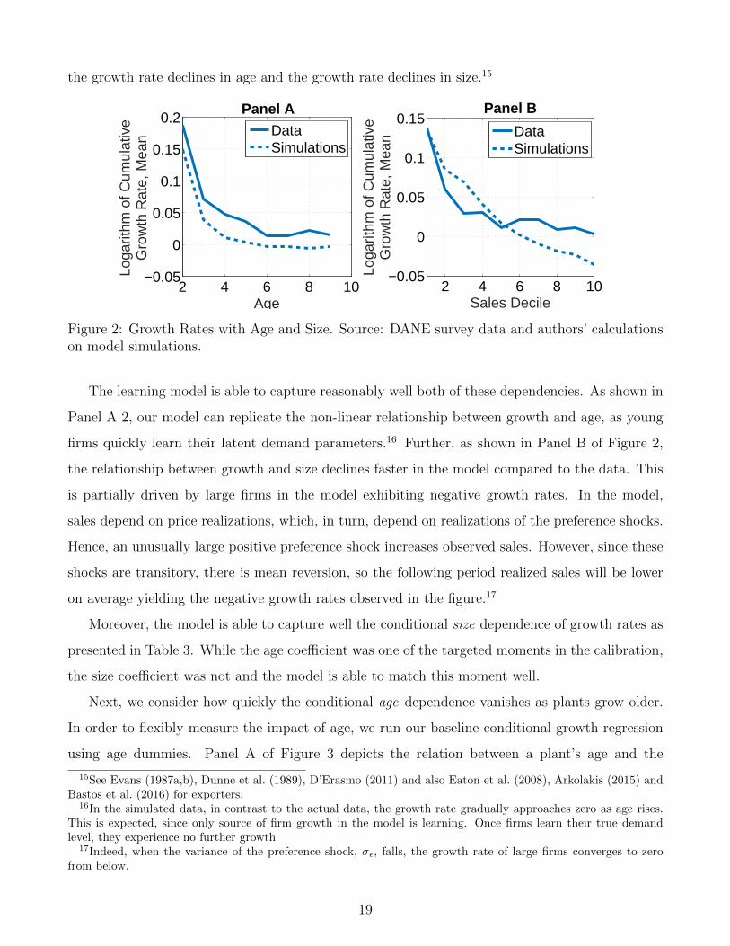
Figure 5 depicts the behavior of aggregate variables along the transition path. At the end of
period 1 the government announces the subsidy policy which will be implemented at the start of
period 2. As can be seen from Panel A of Figure 5, upon the announcement of the policy, real
consumption declines by about 0.34% in the initial transition period. It takes about 15 periods for
the change in aggregate consumption to become positive. When consumption has converged to its
new steady state level, there is a 0.48% increase in consumption compared to the previous steady
state, as indicated in the previous section. Taking into account however the transitional dynamics
depicted in Figure 5, leads to a 0.08% increase in the present discounted stream of consumption.21
Panels B through E of Figure 5 provide further intuition for the transition dynamics behavior.
The consumer-surplus effect is demonstrated in Panel B which depicts the equilibrium mass of
firms. The mass of firms sharply increases in period 2, primarily due to an immediate increase in
entry demonstrated in Panel C, and subsequently continues to increase due to the higher survival
rate of subsidized firms. The profit-destruction effect is demonstrated in Panel D of Figure 5 which
depicts the equilibrium level of income. The equilibrium level of income rapidly declines in the
initial periods, and then converges to its new steady state. In contrast, as demonstrated in Panel
20For computational purposes, we impose τ = 1 for n ≥ 10. The optimal policy results are quantitatively similarfor imposing a higher age threshold and are available upon request.
21Note that in the previous section we search for an optimal policy to maximize static welfare, not taking intoaccount the transitional dynamics. A welfare maximizing planner who takes into account transitional dynamics canpotentially obtain larger (dynamic) welfare gains. However, solving such a problem is computationally infeasible.
23
E, the price level converges to its new level at a much slower pace. These effects jointly lead to a
rapid decline in welfare in the initial periods, and a subsequent increase in welfare driven by the
continuously declining price level, as more profitable firms survive for longer and the share of (less
profitable) entrants declines.
0 10 20 30 40 50Period
-0.6
-0.4
-0.2
0
0.2
0.4
0.6
0.8
Rea
l Con
sum
ptio
n(p
erce
nt in
crea
se)
Panel A
0 10 20 30 40 50Period
0
2
4
6
8
10
12
14
16
18
The
Mas
s of
Firm
s(p
erce
nt in
crea
se)
Panel B
0 10 20 30 40 50Period
8
9
10
11
12
13
14
15
16
The
Shar
e of
Ent
rant
s(p
erce
nt)
Panel C
0 10 20 30 40 50Period
-1.2
-1
-0.8
-0.6
-0.4
-0.2
0Eq
uilib
rium
Inco
me
(per
cent
incr
ease
)Panel D
0 10 20 30 40 50Period
-1.8
-1.6
-1.4
-1.2
-1
-0.8
-0.6
-0.4
-0.2
0
Equi
libriu
m P
rice
Leve
l(p
erce
nt in
crea
se)
Panel E
Figure 5: Transition Dynamics. Values in Panels A, B, D, and E represent percent changes relativeto the corresponding values in the general equilibrium of the learning model. Authors’ calculationson model simulations.
24

4 Conclusion
In this paper we develop a framework to evaluate the importance of learning for firm growth by
suitably adapting the standard learning mechanism of Jovanovic (1982) into an environment with
firm productivity heterogeneity Our setup captures the dependence of growth rates on age, even
conditional on firm size. We characterize the planner’s problem and show that any inefficiency
in this economy is driven by a discrepancy in the firm entry and exit thresholds. Guided by a
theoretical results, we calibrate our setup and show how age-dependent subsidies can be welfare
enhancing, as they allow young firms to avoid early exit and thus benefit consumers through access
to a larger number of varieties.
25

References
Abbring, J. H. and J. R. Campbell (2003): “A Structural Empirical Model of Firm Growth, Learning,and Survival,” NBER working paper, 9712.
Acemoglu, D., U. Akcigit, N. Bloom, and W. Kerr (2013): “Innovation, Reallocation andGrowth,” Tech. rep., National Bureau of Economic Research.
Albornoz, F., G. Corcos, E. Ornelas, and H. F. C. Pardo (2012): “Sequential Exporting,”Journal of International Economics, 88, 17–31.
Arkolakis, C. (2015): “A Unified Theory of Firm Selection and Growth,” mimeo, Yale University.
Atkeson, A. and A. Burstein (2010): “Aggregate Implications of Innovation Policy,” mimeo.
Bastos, P., D. A. Dias, and O. A. Timoshenko (2016): “Learning, Prices, and Firm Dynamics,”mimeo.
Bergemann, D. and J. Valimaki (2000): “Experimentation in markets,” The Review of EconomicStudies, 67, 213–234.
Broda, C. and D. Weinstein (2006): “Globalization and the Gains from Variety,” Quarterly Journalof Economics, 121, 541–585.
Castro, R., G. L. Clementi, and D. Corbae (2004): “Information and Firm Dynamics,” Manuscript,University of Texas at Austin.
Chaney, T. (2008): “Distorted Gravity: The Intensive and Extensive Margins of International Trade,”American Economic Review, 98, 1707–1721.
Clementi, G. L. and B. Palazzo (2013): “Entry, exit, firm dynamics, and aggregate fluctuations,”NBER working paper, 19217.
Commision, E. (2010): “Communication from the Commision to the European Parliament, the Coun-cil, the European Economic and Social Committee and the Committee of the Regions,” EuropeanCommission.
Cooley, T. F. and V. Quadrini (2001): “Financial Markets and Firm Dynamics,” American EconomicReview, 91, 91.
David, J. M., H. A. Hopenhayn, and V. Venkateswaran (2016): “Information, Misallocation, andAggregate Productivity,” Quarterly Journal of Economics, 131, 943–1005.
D’Erasmo, P. (2011): “Investment and firm dynamics,” Available at SSRN 994663.
Dhingra, S. and J. Morrow (2012): “The Impact of Integration on Productivity and Welfare Distor-tions Under Monopolistic Competition,” mimeo, LSE.
Doms, M. and T. Dunne (1998): “Capital Adjustment Patterns in Manufacturing Plants,” Review ofEconomic Dynamics, 1, 409–429.
Dunne, T., M. J. Roberts, and L. Samuelson (1989): “The Growth and Failure of U.S. Manufac-turing Plants,” Quarterly Journal of Economics, 104, 671–698.
Eaton, J., M. Eslava, C. J. Krizan, M. Kugler, and J. Tybout (2012): “A Search and LearningModel of Export Dynamics,” Manuscript, Pennsylvania State University.
Eaton, J., M. Eslava, M. Kugler, and J. Tybout (2008): “The Margins of Entry Into ExportMarkets: Evidence from Colombia,” in Globalization and the Organization of Firms and Markets, ed.by E. Helpman, D. Marina, and T. Verdier, Massachusetts: Harvard University Press.
26

Ericson, R. and A. Pakes (1998): “Empirical Implications of Alternative Models of Firm Dynamics,”Journal of Economic Theory, 79, 1–45.
Evans, D. S. (1987a): “The Relationship Between Firm Growth, Size, and Age: Estimates for 100Manufacturing Industries,” The Journal of Industrial Economics, 35, 567–581.
——— (1987b): “Tests of Alternative Theories of Firm Growth,” The Journal of Political Economy, 95,657–674.
Fitzgerald, D., S. Haller, and Y. Yedid-Levi (2016): “How Exporters Grow,” Manuscript, FederalReserve Bank of Minneapolis.
Grossman, G. and E. Helpman (1991): Innovation and Growth in the Global Economy, Cambridge,Massachussets: MIT press.
Haltiwanger, J., R. Jarmin, and J. Miranda (2013): “Who Creates Jobs? Small Vs. Large Vs.Young,” The Review of Economics and Statistics, 95, 347–361.
Heer, B. and A. Maussner (2009): Dynamic General Equilibrium Modeling: Computational Methodsand Application, Springer.
Hopenhayn, H. A. (1992): “Entry, Exit, and Firm Dynamics in Long Run Equilibrium,” Econometrica,60, 1127–1150.
Itskhoki, O. and B. Moll (2015): “Optimal Development Policies with Financial Frictions,” mimeo,Princeton University.
Jovanovic, B. (1982): “Selection and the Evolution of Industry,” Econometrica, 50, 649–670.
Klette, J. and S. Kortum (2004): “Innovating Firms and Aggregate Innovation,” Journal of PoliticalEconomy, 112, 986–1018.
Luttmer, E. G. J. (2007): “Selection, Growth, and the Size Distribution of Firms,” Quarterly Journalof Economics, 122, 1103–1144.
Melitz, M. J. (2003): “The Impact of Trade on Intra-Industry Reallocations and Aggregate IndustryProductivity,” Econometrica, 71, 1695–1725.
OECD (2013): “OECD Science, Technology and Industry Scoreboard 2013,” OECD Publishing.
Roberts, M. J. (1996): Colombia, 1977-85: Producer Turnover, Margins, and Trade Exposure, Oxford,UK: Oxford University Press, 227–259.
Ruhl, K. J. and J. Willis (2014): “New Exporter Dynamics,” Manuscript New York University.
Timoshenko, O. A. (2015): “Product Switching in a Model of Learning,” Journal of InternationalEconomics, 95, 233–249.
27
A Positive Implications - Expected Growth Rate
Proof of Proposition 1: Expected growth rate conditional on size
The expected growth rate of a firm with current size qt is given by
Ea′
(qt+1(z, a′, n+ 1)
qt(z, a, n)
)=Ea′ (qt+1(z, a′, n+ 1))
qt(z, a, n). (20)
Using equation (7), we can substitute in for the firm’s quantity choice each period to obtain
Ea′ (qt+1(z, a′, n+ 1))
qt(z, a, n)=Ea′((
σ−1σ
)σ ( bt+1(a′,n+1)ez
w
)σY
P 1−σ
)(σ−1σ
)σ ( bt(a,n)ez
w
)σY
P 1−σ
=
(σ−1σ
)σ ( ezw
)σEa′ (bt+1(a′, n+ 1)σ) Y
P 1−σ(σ−1σ
)σ ( bt(a,n)ez
w
)σY
P 1−σ
=Ea′ (bt+1(a′, n+ 1)σ)
bt(a, n)σ.
Denote bt+1(a′, n+ 1) by b′, and bt(a, n) by b. We know that (bσ)′ is log normally distributed, with
mean
mn = log (bσ)−v2n − v2
n+1
2σ
and variance given by
s2n =
λ2 (v2n + σ2
ε)
(1 + (n+ 1)λ)2
where
λ =σ2θ
σ2ε
and
v2n =
σ2θσ
2ε
σ2ε + nσ2
θ
=λσ2
ε
1 + nλ
and n is the firm’s age (number of observations).
Thus the expected growth rate is given by
Ea′
(qt+1
qt
)=Ea ((bσ)′)
bσ=
exp(mn + s2n
2
)bσ
=
bσ exp
(12
λ2(v2n+σ2ε)
(1+(n+1)λ)2− v2n−v2n+1
2σ
)bσ
=
exp
(1
2
λ2 (v2n + σ2
ε)
(1 + (n+ 1)λ)2 −v2n − v2
n+1
2σ
).
Straightforward calculations show that we can rewrite the above growth rate as
exp
(λ2σ2
ε (σ − 1)
2σ (1 + nλ) (1 + (n+ 1)λ)
).
28
The derivative of the above growth rate with age (n) gives
∂ exp(
λ2σ2ε(σ−1)
2σ(1+nλ)(1+(n+1)λ)
)∂n
= exp
(λ2σ2
ε (σ − 1)
2σ (1 + nλ) (1 + (n+ 1)λ)
) ∂(
λ2σ2ε(σ−1)
2σ(1+nλ)(1+(n+1)λ)
)∂n
= − exp
(λ2σ2
ε (σ − 1)
2σ (1 + nλ) (1 + (n+ 1)λ)
)2σλ2σ2
ε (σ − 1)(2λ+ 2nλ2 + λ2
)(2σ (1 + nλ) (1 + (n+ 1)λ))2 < 0
since σ > 1 and all other parameters are positive.
Proof of Proposition 2: Expected growth rate conditional on age and survival
As discussed in Section 2.3, a firm’s state is given by the triplet (z, a, n). The solution to the
firm’s entry and exit problem described in (11) determines a set of market participation thresholds.
Denote by a∗(n, z) such market participation thresholds, such that firm (z, n) stays in the market
if a ≥ a∗(n, z). Hence, the expected growth rate conditional on survival can be written as
Ea′
(qt+1(z, a′, n+ 1)
qt(z, a, n)|a′ ≥ a∗(n+ 1, z), a, n
)=
= Ea′
(σ−1σ
)σ ( b(a′,n+1)ez
w
)σY
P 1−σ(σ−1σ
)σ ( b(a,n)ez
w
)σY
P 1−σ
|a′ ≥ a∗(n+ 1, z), a, n
=
= Ea′
((b(a′, n+ 1))σ
(b(a, n))σ|a′ ≥ a∗(n+ 1, z), a, n
)From equations (4) and (8), b(a, n) is monotonically increasing in a based on our assumption of
the normal prior and shocks. Hence, the conditional expected growth rate can be written as
Eb′
((b′)σ
bσ|b′ ≥ b∗(n+ 1, z), a, n
), (21)
where (b′)σ/bσ is log-normally distributed with mean and variance independent of size, as a result of
our assumption of the normal prior and shocks. From Proposition 1 in Timoshenko (2015) we know
that in this environment a∗(n + 1, z), and therefore b∗(n + 1, z)σ, are declining in z. Therefore
expression 21 is a conditional expectation of a positive random variable whose distribution is
independent of size. The lower threshold of this integration is b∗ and thus is declining in size.
Thus, conditional on age and survival, the expected growth rate declines in size.
29
B Normative Implications
We start by setting up the planner’s problem in its full detail. Before introducing the problem
it is useful to introduce some notation. Denote by I(z, a, n) ∈ 0, 1 the exit/stay decision of
the planner for the incumbents of type (z, a, n) and by N(z) ∈ 0, 1 the exit/entry decision for
entrants of type (z). Denote by qP (z, a, n) and by qPe (z) the quantity produced by the incumbents
of type (z, a, n) and entrants of type (z) respectively. Let m(z, a, n) denote the mass of firms in
state (z, a, n). Finally, h(a|ˆa, n) denotes the density function which corresponds to the transition
of a firm whose age is n and current average demand realization is ˆa moving to average demand
realization of a. In other words, it is the density corresponding to obtaining a demand realization
a = (n+ 1)a− nˆa.22
Since there is no aggregate shocks or aggregate uncertainty we focus on the stationary planner
problem given by
maxI(z,a,n),N(z),qP (z,a,n),qPe (z)
lnC∗ (23)
subject to
C∗ =
(∞∑n=1
∫z
∫a
qP (z, a, n)σ−1σ b(a, n)I(z, a, n)m(z, a, n)dadz +
∫z
qPe (z)σ−1σ b0N(z)g(z)dz
) σσ−1
(24)
∞∑n=1
∫z
∫a
(qP (z, a, n)
ez+ f
)I(z, a, n)m(z, a, n)dadz +
∫z
(qPe (z)
ez+ f
)N(z)g(z)dz ≤ L (25)
m(z, a, n+ 1) =
∫ˆa
(1− δ)I(z, ˆa, n)m(z, ˆa, n)h(a|ˆa, n)dˆa, (26)
22Since the belief of a firm regarding the realization of its demand shock a follows N(µn, ν2n + σ2
ε) then h(a|ˆa, n)is given by
h(a|ˆa, n) =1√
υ2n + σ2ε
φ
(a(n+ 1)− ˆan− µn(ˆa)√
υ2n + σ2ε
), (22)
where φ(.) denotes the probability density of the standard Normal distribution.
30

m(z, 0, 0) = J ·N(z) · g(z) (27)
The first constraint, equation (24), follows from the definition of the consumption aggregate
and the stationary steady state assumption wherein we have replaced the preference shocks in
the utility term by their expected values. The second constraint, equation (25), is the resource
constraint for labor. The last two constraints, equations (26) and (27), are the mass balance
conditions in the stationary steady state equilibrium.
Since we assume Bayesian learning, firm beliefs are set to
b(a, n) = Ea|a,neaσ = exp
µnσ
+1
2
(ν2n + σ2
ε
σ2
)and
b0 = Ea|0,0eaσ = exp
θ
σ+
1
2
(σ2θ
σ2
).
Quantity Decision
We first solve for the optimal quantity decisions by the planner taking the entry and exit
decisions as given. Let λ denote the Lagrange multiplier on the resource constraint, equation (25).
The first order condition with respect to qP (z, a, n) yields(C∗
1−σσ qP (z, a, n)
−1σ b(a, n)− λ
ez
)m(z, a, n)I(z, a, n) = 0
⇒ qP (z, a, n) =
(ezb(a, n)
λC∗σ−1σ
)σ, for n ≥ 1. (28)
Similarly, the first order condition with respect to qPe (z) yields
qPe (z) =
(ezb0
λC∗σ−1σ
)σ, (29)
We now solve for the two endogenous unknowns C∗ and λ. Substituting the optimal quantity
decisions (28) and (29) into the consumption aggregate equation (24) yields
C∗ =
(∞∑n=1
∫z
∫a
(ezb(a, n)
λC∗σ−1σ
)σ−1
b(a, n)I(z, a, n)m(z, a, n)dadz +
∫z
(ezb0
λC∗σ−1σ
)σ−1
b0N(z)g(z)dz
) σσ−1
.
31

The equation simplifies to
(λC∗)σ =
(∞∑n=1
∫z
∫a
ez(σ−1) (b(a, n))σ I(z, a, n)m(z, a, n)dadz +
∫z
ez(σ−1) (b0)σN(z)g(z)dz
) σσ−1
≡ Aσσ−1
⇒ λ =A
1σ−1
C∗. (30)
Next, substituting the optimal quantities into the resource condition for labor, equation (25),
and noting that the second term represents the total mass of firms we obtain
A
λσC∗σ−1+ fM = L
C∗1−σ
λσ=L− fM
A. (31)
Solving equations (30) and (31), we obtain
λ =1
L− fM(32)
and
C∗ =L− fMA
11−σ
. (33)
Hence, the optimal quantity decisions for all the active firms in the economy are given by
qP (z, a, n) =(ezb(a, n))σ (L− fM)
A, for n ≥ 1 (34)
qPe (z) =(ezb0)σ (L− fM)
A, (35)
This completes characterization of the optimal quantities chosen by the planner conditional on
entry and exit decisions.
Observe that the quantities derived here are identical (up to a multiplicative constant) to the
ones obtained for the competitive equilibrium case (see equation (7)). Thus, there is no distortion
to the relative quantities of firms that are active in both the decentralized equilibrium and the
planner’s equilibrium. Hence, the main difference between the planner’s and the market allocation
will arise from the equilibrium mass of active firms.
Entry and Exit Decision
Using the results for the optimal quantities obtained above, we can now re-write the planner’s
32

problem as a pure entry and exit problem as follows:
maxI(z,a,n),N(z)
[ln
(L− fMA
11−σ
)], (36)
subject to
M =
(∞∑n=1
∫z
∫a
I(z, a, n)m(z, a, n)dadz +
∫z
N(z)g(z)dz
)(37)
A =∞∑n=1
∫z
∫a
ez(σ−1) (b(a, n))σ I(z, a, n)m(z, a, n)dadz +
∫z
ez(σ−1) (b0)σN(z)g(z)dz (38)
m(z, a, n+ 1) =
∫ˆa
(1− δ)I(z, ˆa, n)m(z, ˆa, n)h(a|ˆa, n)dˆa, (39)
m(z, 0, 0) = J ·N(z) · g(z) (40)
Let the entry and exit decisions of the planner be defined through a cut-off rule as described below.
For every z ∈ Z and n ≥ 1 define aP (z, n) as follows:
I(z, a, n) =
1 ∀a ≥ aP (z, n)
0 otherwise.
Similarly, define zPas
N(z) =
1 ∀z ≥ zP
0 otherwise.
Therefore, the entry and exit choice problem of the planner can be represented as follows:
maxaP (z,n)z,n≥1,zP
[ln
(L− fMA
11−σ
)], (41)
subject to
M =∞∑n=1
(∫ +∞
zP
∫ +∞
aP (z,n)
m(z, a, n)dadz
)+ J ·
∫ +∞
zPg(z)dz (42)
33

A =∞∑n=1
(∫ +∞
zP
∫ +∞
aP (z,n)
ez(σ−1)b(a, n)σm(z, a, n)dadz
)+ J ·
∫ +∞
zPez(σ−1)bσ0g(z)dz (43)
m(z, a, n+ 1) =
∫ +∞
aP (z,n)
(1− δ)m(z, ˆa, n)h(a|ˆa, n)dˆa, (44)
m(z, 0, 0) =
J · E(z) · g(z) z ≥ zP
0 otherwise.
(45)
Substituting equations (42)-(45) into the objective function in the equation (41) and taking
the first order condition with respect to aP (z, n) yields
f
L− fM· ∂M
∂aP (z, n)=
1
A(σ − 1)· ∂A
∂aP (z, n), (46)
where
∂M
∂aP (z, n)=
∫ +∞
zP
(+∞∑k=n
(∫ +∞aP (k,n)
m(z, a, k)da
∂aP (z, n)
))dz and
∂A
∂aP (z, n)=
∫ +∞
zP
(+∞∑k=n
(∫ +∞aP (k,n)
ez(σ−1)b(a, k)σm(z, a, k)da
∂aP (z, n)
))dz.
Equation (46) equates marginal benefit to marginal cost from changing an exit threshold. The
intuition is as follows. When the threshold aP (z, n) increases by a small amount, the mass of firms
who are at the margin exits. Hence, the economy no longer incurs the fixed cost of production for
these exiting firms. The total gain from incurring less fixed costs is captured by the left hand side
of equation (46). The right hand side captures the loss to the aggregate utility from the exit of
firms since consumers now have less available varieties since variable A defined in equation (38) is
the average profitability of firms.
Proof of Corollary 4
Note that the planner’s quantity choices, (17) and (18), are equal to the market’s quantity
choice (7), if (σ − 1
σ
)σY P σ−1
wσ=L− fM
A(47)
and M and A in the stationary economy coincide with those of the planner’s allocation. We first
34

show that in the stationary economy condition (47) holds and then we show that M and A are
the same as in the planner’s allocation.
Substituting the market clearing price (9) into the price index equation (3), we obtain
P 1−σ =
(σ
σ − 1
)1−σ
w1−σA. (48)
The goods market clearing condition can be written as
Y = wL+ vΠ− wfM,
where vΠ is the total variable profit and equals to Y/σ. Hence, Y can be expressed as
Y =σ
σ − 1(wL− wfM). (49)
Substituting equations (48) and (49) into equation (47), we obtain condition (47) above.
In addition, M and A are the same as in the planner’s allocation. To see this, note that from
condition 5 of the equilibrium definition, the equilibrium mass of firms, M , is determined by the
corresponding mass of firms of each type, (z, a, n), which is determined by the entry and exit
threshold. Hence if the entry and exit thresholds are the same, so will the the total mass of firms,
M . Finally, from equation (38), A is also determined by the density of firms of each type, (z, a, n),
which is the same as in the planner’s allocation if the thresholds are the same. Thus when the
entry and exit thresholds are the same, so are the quantity decisions.
C Data
The measure of a plant’s sales is taken to be the real value of production (variable RP in the
dataset). The real value of production is reported in thousands of pesos. Thus, all values are
multiplied by 1000.
The first calibrating moment - the mean of the logarithm of sales - is constructed by taking a
cross sectional mean of the logarithm of plants’ sales for a given year. The reported value is the
mean across annual observations between 1983 and 1991.
For the second calibrating moment - the share of sales from entrants - an entrant is defined as
a plant which is observed selling a positive amount in a given period, and is not observed in the
sample in the previous period. The reported value is the mean across annual observations between
1983 and 1991.
35
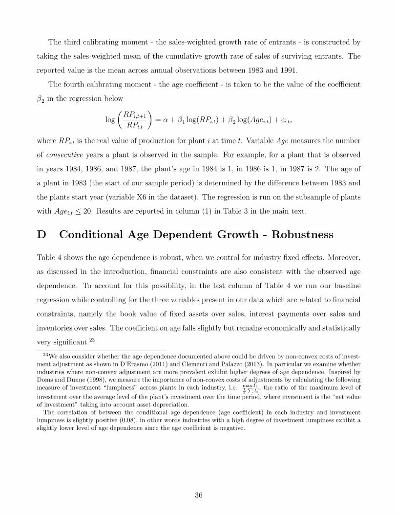
The third calibrating moment - the sales-weighted growth rate of entrants - is constructed by
taking the sales-weighted mean of the cumulative growth rate of sales of surviving entrants. The
reported value is the mean across annual observations between 1983 and 1991.
The fourth calibrating moment - the age coefficient - is taken to be the value of the coefficient
β2 in the regression below
log
(RPi,t+1
RPi,t
)= α + β1 log(RPi,t) + β2 log(Agei,t) + εi,t,
where RPi,t is the real value of production for plant i at time t. Variable Age measures the number
of consecutive years a plant is observed in the sample. For example, for a plant that is observed
in years 1984, 1986, and 1987, the plant’s age in 1984 is 1, in 1986 is 1, in 1987 is 2. The age of
a plant in 1983 (the start of our sample period) is determined by the difference between 1983 and
the plants start year (variable X6 in the dataset). The regression is run on the subsample of plants
with Agei,t ≤ 20. Results are reported in column (1) in Table 3 in the main text.
D Conditional Age Dependent Growth - Robustness
Table 4 shows the age dependence is robust, when we control for industry fixed effects. Moreover,
as discussed in the introduction, financial constraints are also consistent with the observed age
dependence. To account for this possibility, in the last column of Table 4 we run our baseline
regression while controlling for the three variables present in our data which are related to financial
constraints, namely the book value of fixed assets over sales, interest payments over sales and
inventories over sales. The coefficient on age falls slightly but remains economically and statistically
very significant.23
23We also consider whether the age dependence documented above could be driven by non-convex costs of invest-ment adjustment as shown in D’Erasmo (2011) and Clementi and Palazzo (2013). In particular we examine whetherindustries where non-convex adjustment are more prevalent exhibit higher degrees of age dependence. Inspired byDoms and Dunne (1998), we measure the importance of non-convex costs of adjustments by calculating the followingmeasure of investment “lumpiness” across plants in each industry, i.e. max It
1T
∑It
, the ratio of the maximum level of
investment over the average level of the plant’s investment over the time period, where investment is the “net valueof investment” taking into account asset depreciation.
The correlation of between the conditional age dependence (age coefficient) in each industry and investmentlumpiness is slightly positive (0.08), in other words industries with a high degree of investment lumpiness exhibit aslightly lower level of age dependence since the age coefficient is negative.
36

Sales Growth Rate Sales Growth Rate Sales Growth Rate
ln(sales) -0.022 -0.027 -0.026(0.002)∗∗∗ (0.002)∗∗∗ (0.002)∗∗∗
ln(plant age) -0.035 -0.033 -0.030(0.002)∗∗∗ (0.002)∗∗∗ (0.002)∗∗∗
Industry Fixed Effects X XLeverage/Financial Dependence Controls X
R2 0.02 0.02 0.03Number of Observations 36,877 36,877 36,877
Table 4: Growth dependence on Age and Size. Financial variables are the book value of fixedassets over sales, interest payments over sales and inventories over sales. Standard errors clusteredby plant. ∗∗∗ denotes significance at the 1% level. Source: DANE survey data (see text for details).
E Solving the Stationary Equilibrium
The computation of the stationary equilibrium is based on the method developed in Timoshenko
(2015). Here we briefly outline the steps for solving for the stationary equilibrium objects:
ez,M, P and Y .
Introduce the following change of variables
uσ−1 =(ez)σ−1P σ−1Y
wσ−1(50)
(u∗)σ−1 =(ez)σ−1P σ−1Y
wσ−1, (51)
where u∗ is a solution to the firm’s entry problem
V (u∗, b0, 0) = 0.
Given u∗, one is able simulate the equilibrium distribution of firms. From the equilibrium distri-
bution we obtain r, the mean revenue of firms, π, the mean profit level of firms, and m(z, a, n),
the distribution of firms across their state variables.
From the goods market clearing condition, we can then solve for the equilibrium mass of firms
as
M =L
r − π.
37

From the exogenous entry condition, we can solve for ez:
M = J
(ezmin
ez
)ξ×Mass
ez =
(J ×Mass
M
) 1ξ
ezmin ,
where, Mass is the mass of firms as determined by m(z, a, n). Next, we can solve for Y and P
from the goods market clearing conditions and equation (51) as follows:
Y = L+Mπ,
P =u∗
Y1
σ−1 ez.
This completes solving for the general equilibrium objects.
F Computation Algorithm for Transition Dynamics
The economy starts in period 1 in the stationary equilibrium. At the start of period 2, the
government announces a fixed costs subsidy program. Denote by Yt and Pt the aggregate income
and price levels in a transition period t. Observe that a firm’s revenue and expected profit depend
on the product of these two aggregate variables given by Xt = YtPσ−1t .24 Given the aggregate
variables summarized by Xt, the static within-period profit maximization problem of a firm remains
unchanged as is described in equation (5). The entry and exit problem of an incumbent firm in a
transition period t is given by
Vt(z, a, n,Xt) = max (Eπ(z, a,Xt) + β(1− δ)EVt+1(z, a′, n+ 1, Xt+1); 0) . (52)
Potential entrants start to produce in period t when their productivity draw is above the entry
threshold zt. The entry threshold is implicitly determined by the entry condition
Vt(zt, a, 0, Xt) = 0. (53)
We solve for the transition path using an algorithm described in Heer and Maussner (2009).25
In the context of our model, the steps are as follows:
1. Let T be the number of transition periods.
24In computing the transitional dynamics, due to the Walras’ law, one price in each period can be normalized.We normalize the wage rate, wt, to 1.
25We adopt Algorithm 6.2.2 described on page 314.
38

2. Guess a time path for the aggregate variable Xt, such that X1 is given by the value from the
initial stationary equilibrium and XT is given by the value from the subsidy equilibrium.
3. Use the backward induction method to solve for the value functions in equations (52) and
(53) for each transition period t.
4. Recover the entry and exit thresholds from the value functions computed in the previous
step.
5. Take the stationary distribution of firms in period 1, and using the computed entry and
exit threshold and firms’ optimal quantity choices according to equation (5), simulate the
distribution of firms in each of the transition periods.
6. Check whether the market clearing condition Yt = L+ Πt +Tt holds in each of the transition
periods, where Πt is the aggregate profit level in period t, and Tt is the total value of the
subsidy payments.
7. If markets do not clear, update Xt.
G Learning Model with Productivity Evolution
In this appendix we modify the learning model to allow for firm productivity, ezt , to change over
time. We also calibrate this extended model with both learning and productivity evolution.
In particular, conditional on a firm’s survival, productivity zt(ω) changes over time according
to
zt (ω) = ρzt−1 (ω) + ut (ω) , ut (ω) ∼ N(0, σ2
u
)i.i.d.
Firms observe this period’s productivity when making their quantity decision, but do not know
next period’s productivity realizations. In addition, today’s quantity choice does not affect the
evolution of productivity. Thus, the firm’s optimal quantity decision is still given by equation (7).
The firm’s value function (dropping the ω and the t) is now given by
V (z, a, n) = maxEπ(z, a, n) + β(1− δ)Ez′|z,a′|a,nV (z′, a′, n+ 1), 0
.
Since productivity now changes over time, firms take this into account both when making their
entry decision, as well as when considering whether to remain in a market or exit. In particular,
39

there is an option value of higher productivity draws in the future, especially given the convexity
of ez.
We now turn to the calibration. As in the calibration of the baseline model we calibrate
some of the parameters independently. In particular, β and δ take the values of 0.9606 and 0.025
respectively, while the autocorrelation coefficient, ρ, is set to 0.999.
The remaining parameters are jointly calibrated. In particular, we calibrate the following five
parameters: the per period fixed cost, f , the standard deviation of shocks to demands, σε, the
shape parameter of the distribution of the initial productivity draws, ξ, the standard deviation of
the distribution of the unobserved demand parameter, σθ and the standard deviation of shocks to
productivity, σu. We use the following five moments: mean log sales, the standard deviation of
log sales, the sales-weighted growth rate of entrants, the entrants’ share of sales and the annual
survival rate.
As in the baseline model, it is impossible to provide a rigorous identification argument, but we
offer an informal argument of how each parameter is identified from the data. The per period fixed
cost, f , is pinned down by mean log sales, since increasing the fixed cost pushes less productive
firms out of the market increasing mean sales. The standard deviation of log sales informs us about
the standard deviation of the distribution of the unobserved demand, σθ, since higher dispersion in
that distribution translates into a more disperse sales distribution. The shape of the distribution
of the initial productivity draws, ξ, is pinned down by entrants’ share of sales: A lower value for ξ,
all else equal, leads to a higher initial productivity dispersion and therefore more entrants starting
off relatively large. Finally, the sales-weighted growth rate of entrants and the annual survival
rate identify the standard deviation of shocks to demand, σε and the standard deviation of shocks
to productivity, σu. Intuitively, a lower σε implies faster learning and therefore, all else equal,
low demand firms exit sooner, while surviving firms grow faster. Similarly, a higher dispersion of
productivity shocks, σu, leads to both a higher exit rate, as more firms are hit by large negative
shocks, but also higher growth rates. Therefore the growth and survival moments allow us to
identify these two moments.
The calibrated parameters are presented in Table 5 and the targeted moments are presented
in Table 6. Two comments are in order: First the fit of the model is quite good, with all moments
quite close to their targets. In addition as shown in Table 6, the model also matches the size
coefficient of the regression of growth of sales on age and size. This moment was not targeted in
40

Parameter Value
ξ 10.80σε 1.32σθ 0.95σu 0.02f 248,572
Table 5: Parameter Values for the Learning Model with Productivity Evolution. Source: ModelCalibration with Productivity Evolution
Targeted Moments: Data Productivity Model No Productiv. Evolution
Mean of Log-Sales 14.99 15.09 15.08Share of Sales from Entrants 2.66% 2.65% 2.50%
Sales-Weighted Growth Rate of Entrants 23% 21% 19%Age Coefficient -0.035 -0.035 -0.032
Annual Survival Rate 91% 90% 92%Other Moment:
Size Coefficient -0.022 -0.023 -0.017
Table 6: Data and Simulation Moments for the Learning Model with Productivity Evolution.Sources: DANE survey data (see text for details); Model calibration with productivity evolution;Counterfactual model simulation when zt+1 = zt
the calibration and nonetheless the fit is close to exact.
Second, the calibrated parameters indicate that most of the action is driven by learning rather
than productivity. Indeed the standard deviation of productivity shocks, σu, necessary to match
the data is very small, especially compared to the two parameters capturing the importance of
learning, σε and σθ.
This becomes even more apparent when we use the calibrated model with productivity growth
and shut down the productivity evolution channel (set zt = z0 for all t). The resulting moments
are presented in the last column of Table 6. Notice, that with the exception of the size coefficient,
all other moments do not change much. In particular, the age coefficient changes by less than
ten percent suggesting that learning is the key mechanism in accounting for the conditional age
dependence of growth rates. The absolute value of the size coefficient however, declines by almost
a third indicating that time-varying productivity plays a much larger role in accounting for the
conditional size (rather than age) dependence of growth rates.
41