fire dynamics simulator : user's manual · nistir 6469 fire dynamics simulator - user’s...
TRANSCRIPT

Fire Dynamics Simulator –User’s Manual
Kevin B. McGrattanGlenn P. Forney
NISTIR 6469

NISTIR 6469
Fire Dynamics Simulator -User’s Manual
Kevin B. McGrattanGlenn P. Forney
Building and Fire Research Laboratory
January 2000
U.S. Department of CommerceWilliam M. Daley, Secretary
Technology AdministrationDr. Cheryl L. Shavers, Under Secretary of Commerce for Technology
National Institute of Standards and TechnologyRaymond G. Kammer, Director

Disclaimer
The US Department of Commerce makes no warranty, expressed or implied, to users of the Fire Dy-namics Simulator (FDS), and accepts no responsibility for its use. Users of FDS assume sole responsibilityunder Federal law for determining the appropriateness of its use in any particular application; for any con-clusions drawn from the results of its use; and for any actions taken or not taken as a result of analysesperformed using these tools.
Users are warned that FDS is intended for use only by those competent in the fields of fluid dynamics,thermodynamics, combustion, and heat transfer, and is intended only to supplement the informed judgmentof the qualified user. The software package is a computer model that may or may not have predictivecapability when applied to a specific set of factual circumstances. Lack of accurate predictions by the modelcould lead to erroneous conclusions with regard to fire safety. All results should be evaluated by an informeduser.
Throughout this document, the mention of computer hardware or commercial software does not con-stitute endorsement by NIST, nor does it indicate that the products are necessarily those best suited for theintended purpose.
ii

Contents
1 Getting Started 11.1 How to get FDS . . . . . . . . . . . . . . . . . . . . . . . . . . . . . . . . . . . . . . . . . 11.2 Computer Hardware Requirements . . . . . . . . . . . . . . . . . . . . . . . . . . . . . . . 1
2 Running fds 22.1 Compiling the Source Code . . . . . . . . . . . . . . . . . . . . . . . . . . . . . . . . . . . 22.2 Creating the data file . . . . . . . . . . . . . . . . . . . . . . . . . . . . . . . . . . . . . . 32.3 Running fds . . . . . . . . . . . . . . . . . . . . . . . . . . . . . . . . . . . . . . . . . . . 32.4 Monitoring Progress . . . . . . . . . . . . . . . . . . . . . . . . . . . . . . . . . . . . . . 3
3 Running Smokeview 53.1 Getting Started . . . . . . . . . . . . . . . . . . . . . . . . . . . . . . . . . . . . . . . . . 53.2 Installation . . . . . . . . . . . . . . . . . . . . . . . . . . . . . . . . . . . . . . . . . . . 53.3 Menu Options . . . . . . . . . . . . . . . . . . . . . . . . . . . . . . . . . . . . . . . . . . 53.4 Keyboard Commands . . . . . . . . . . . . . . . . . . . . . . . . . . . . . . . . . . . . . . 63.5 Command Line Options . . . . . . . . . . . . . . . . . . . . . . . . . . . . . . . . . . . . . 63.6 Customization Files . . . . . . . . . . . . . . . . . . . . . . . . . . . . . . . . . . . . . . . 8
4 Case Studies 114.1 Isolated Fire Plume . . . . . . . . . . . . . . . . . . . . . . . . . . . . . . . . . . . . . . . 114.2 Smoke Movement in a Townhouse . . . . . . . . . . . . . . . . . . . . . . . . . . . . . . . 164.3 Sprinkler Study . . . . . . . . . . . . . . . . . . . . . . . . . . . . . . . . . . . . . . . . . 18
4.3.1 Experimental Description . . . . . . . . . . . . . . . . . . . . . . . . . . . . . . . 184.3.2 Simulation Parameters . . . . . . . . . . . . . . . . . . . . . . . . . . . . . . . . . 204.3.3 Results . . . . . . . . . . . . . . . . . . . . . . . . . . . . . . . . . . . . . . . . . 22
4.4 Large Outdoor Fires . . . . . . . . . . . . . . . . . . . . . . . . . . . . . . . . . . . . . . . 244.5 Rack Storage Fire . . . . . . . . . . . . . . . . . . . . . . . . . . . . . . . . . . . . . . . . 27
5 Glossary of Input Parameters 305.1 The HEAD Namelist Group . . . . . . . . . . . . . . . . . . . . . . . . . . . . . . . . . . . 305.2 The GRID Namelist Group . . . . . . . . . . . . . . . . . . . . . . . . . . . . . . . . . . . 315.3 The PDIM Namelist Group . . . . . . . . . . . . . . . . . . . . . . . . . . . . . . . . . . . 315.4 The TRNX, TRNY and/or TRNZ Namelist Groups . . . . . . . . . . . . . . . . . . . . . . . 315.5 The TIME Namelist Group . . . . . . . . . . . . . . . . . . . . . . . . . . . . . . . . . . . 335.6 The MISC Namelist Group . . . . . . . . . . . . . . . . . . . . . . . . . . . . . . . . . . . 335.7 The SPEC and REAC Namelist Groups . . . . . . . . . . . . . . . . . . . . . . . . . . . . . 345.8 The SURF Namelist Group . . . . . . . . . . . . . . . . . . . . . . . . . . . . . . . . . . . 36
5.8.1 Thermal Boundary Conditions . . . . . . . . . . . . . . . . . . . . . . . . . . . . . 365.8.2 Velocity Boundary Condition . . . . . . . . . . . . . . . . . . . . . . . . . . . . . 365.8.3 Prescription of a Fire (LES only) . . . . . . . . . . . . . . . . . . . . . . . . . . . . 375.8.4 Species Boundary Conditions . . . . . . . . . . . . . . . . . . . . . . . . . . . . . 385.8.5 Time Dependent Boundary Conditions . . . . . . . . . . . . . . . . . . . . . . . . . 39
5.9 The OBST Namelist Group . . . . . . . . . . . . . . . . . . . . . . . . . . . . . . . . . . . 395.10 The VENT Namelist Group . . . . . . . . . . . . . . . . . . . . . . . . . . . . . . . . . . . 405.11 The SPRK Namelist Group . . . . . . . . . . . . . . . . . . . . . . . . . . . . . . . . . . . 405.12 The HEAT Namelist Group . . . . . . . . . . . . . . . . . . . . . . . . . . . . . . . . . . . 41
iii

5.13 The PART Namelist Group . . . . . . . . . . . . . . . . . . . . . . . . . . . . . . . . . . . 415.14 The THCP Namelist Group . . . . . . . . . . . . . . . . . . . . . . . . . . . . . . . . . . . 425.15 The PL3D Namelist Group . . . . . . . . . . . . . . . . . . . . . . . . . . . . . . . . . . . 435.16 The SLCF Namelist Group . . . . . . . . . . . . . . . . . . . . . . . . . . . . . . . . . . . 435.17 The BNDF Namelist Group . . . . . . . . . . . . . . . . . . . . . . . . . . . . . . . . . . . 44
6 Output File Formats 456.1 Diagnostic Output . . . . . . . . . . . . . . . . . . . . . . . . . . . . . . . . . . . . . . . . 456.2 PLOT3D Data . . . . . . . . . . . . . . . . . . . . . . . . . . . . . . . . . . . . . . . . . . 456.3 Thermocouple Data . . . . . . . . . . . . . . . . . . . . . . . . . . . . . . . . . . . . . . . 466.4 Sprinkler Data . . . . . . . . . . . . . . . . . . . . . . . . . . . . . . . . . . . . . . . . . . 466.5 Heat Release Rate . . . . . . . . . . . . . . . . . . . . . . . . . . . . . . . . . . . . . . . . 476.6 Slice Files . . . . . . . . . . . . . . . . . . . . . . . . . . . . . . . . . . . . . . . . . . . . 476.7 Boundary Files . . . . . . . . . . . . . . . . . . . . . . . . . . . . . . . . . . . . . . . . . 476.8 Particle Data . . . . . . . . . . . . . . . . . . . . . . . . . . . . . . . . . . . . . . . . . . . 48
7 Conclusion 50
References 51
iv

1 Getting Started
Fire Dynamics Simulator (FDS) is a computational fluid dynamics (CFD) model of fire-driven fluid flow.The software described in this document solves numerically a form of the Navier-Stokes equations appro-priate for low-speed, thermally-driven flow with an emphasis on smoke and heat transport from fires. Theformulation of the equations and the numerical algorithm are contained in a companion document, calledFire Dynamics Simulator – Technical Reference Guide [1]. The intent of this User’s Manual is to explainhow calculations are performed and how to analyze the results.
Fire Dynamics Simulator consists of two computer programs. The first, called simply fds, is a Fortran90 computer program that solves the equations described in Ref. [1]. The second, called smokeview, is anOpenGL graphics program that allows one to visualize the results. All of the input parameters required byfds to describe the particular scenario of interest are conveyed via one or two text files created by the user.Version 1 of smokeviewhas a limited Graphical User Interface (GUI), with major parameters controlled bya GUI and minor parameters controlled via a text file.
1.1 How to get FDS
All of the files associated with FDS are linked to the URL
http://fire.nist.gov
The FDS distribution consists of the Fortran 90 source code for fds, a compiled executable for the PC(fds.exe), a compiled executable of smokeview for the PC (smokeview.exe) and several popular UNIXworkstations, and sample input files for the cases discussed below.
1.2 Computer Hardware Requirements
Fire Dynamics Simulator requires a relatively fast CPU and a substantial amount of random-access memory(RAM). Both fds and smokevieware portable and can be run on a variety of computing platforms. Fora Windows-based PC, the processor should be at least as fast as a 450 Mhz Pentium II, with at least 256Mbytes of memory. Of course, more is better, but this configuration should allow the user to do fairly largecalculations in a reasonable time period. For UNIX-based workstations, the processor and memory shouldbe at least as fast and as large as the PC specs.
1

2 Running fds
Running fds is relatively simple. All of the parameters that describe a given fire scenario are typed intoa text file that will be referred to as the “data” file. In this document, the data file will be designatedas casename.data. In practice, the user chooses the identifying string “casename” so that all of the filesassociated with a given calculation all have a common prefix. A second text file, referred to as the “database”file, contains parameters describing specific materials, sprinklers, and other devices that can be referred toby name in the data file. In Section 4, several data files will be presented, along with entries pulled from thedatabase file. It is suggested that a new user start with an existing data file and make the appropriate changesto reflect the desired scenario.
2.1 Compiling the Source Code
If a compiled version of fds exists for the machine on which the calculation is to be run, there is no need tocompile the code, and this section may be skipped. For example, the file fds.exeis the compiled programfor a Windows-based PC; thus PC users do not need a Fortran compiler and do not need to compile thesource code. For machines for which an executable has not been compiled, the user must compile the code.A Fortran 90 compiler is needed for compilation. Table 1 lists the files that make up the source code. Thesefiles contain fixed form Fortran 90 instructions conforming to the ANSI and ISO standards except for themachine-specific instructions found in the files named sys ***.f . Before compiling, the user should selectthe sys ***.f file that is appropriate for the operating system of the machine on which the program will becompiled and run. Presently, there are machine-specific files for IBM AIX (sys aix.f), SGI IRIX (sys irix.f ),SUN Solaris (sys sol.f), DEC UNIX (sys dec.f), and Digital Visual Fortran (sys dvf.f). These files containtiming and buffer flushing calls that are not standard in Fortran 90 and differ from machine to machine. Ifnone of the available files is appropriate, the user should either use sys gen.fas is, or modify it appropriately.The source files should be compiled in the order in which they are listed in Table 1 because some routinesare dependent on others. For UNIX users, a Makefile has been provided that will assist in the compilation.Compiler options differ from platform to platform. The only compiler options that need to be prescribed arethose that optimize performance.
Table 1: Source Code Files
File Name Description
mods.f Global arrays and constantssys ***.f Machine-specific timing, flushing routines
read.f Read input parametersinit.f Initialize variables and Poisson solverdivg.f Compute the flow divergencemass.f Mass equation(s) and thermal boundary conditionspres.f Spatial discretization of pressure (Poisson) equationpois.f Poisson solvervelo.f Momentum equationspart.f Thermal elements and combustionsprk.f Sprinkler activation and spray dynamicsdump.f Dumps output data into files
main.f Main program, calls subroutines
2

2.2 Creating the data file
The data file provides the program with all of the necessary information to describe the scenario underconsideration. The most important inputs determine the physical size of the overall rectangular domain,the grid dimensions, and the additional geometrical features. Next, the energy sources must be prescribedand other boundary conditions. Finally, there are a number of parameters that customize the output filesto capture the most important flow quantities. Input data is prescribed by writing a small file containingFortran NAMELIST formatted records. Each record consists of a line or lines in the data file beginningwith the character & followed immediately by the name of the NAMELIST group (HEAD, GRID, VENT,etc.), followed by a list of the input parameters corresponding to that group. Each list is terminated with aslash. Note that the parameters listed are only those that the user desires to be changed from the default. AGlossary of Input parameters is found in Section 5 along with several sample data files in Section 4. It isrecommended that a new user simply execute one of the sample cases that best resembles the scenario ofinterest, and then modify that sample case appropriately. By doing this, the user will quickly learn how tocreate a data file.
2.3 Running fds
Windows: Open up a DOS shell session, and change directories to where the data file for the case is, thenrun the code by typing
fds < casename.data
to begin a run. The character string casename is the name of the case designated in the user-generatedinput file called casename.data. The input parameters will be read in as standard input, and the diagnosticoutput will be written out onto the screen. If one desires to save the diagnostic output, the job should be run
fds < casename.data > casename.out
The diagnostic output will then be saved to a file called casename.out. This file can be checked periodicallyto monitor the progress of the calculation.
UNIX: Change directories to where the data file for the case is, then run the code by typing
fds < casename.data > casename.out &
to begin a run. The input parameters will be read in as standard input, and the diagnostic output will bewritten out as standard output to a file called casename.out. To watch the progress of a run on the screen,simply type
fds < casename.data
Note that in the latter case, the job will be run in the foreground and the diagnostic output will not be saved.It is preferable to run jobs in the background so that a record of the calculation diagnostics will be saved.
2.4 Monitoring Progress
Diagnostics for a given calculation are either written out onto the screen or into a file, usually called case-name.outby the user. The CPU usage and simulation time will be written here, so a user can see how faralong the program has progressed. At any time during a calculation, smokeviewcan be run and the progresscan be checked visually. To stop a calculation before its scheduled time, a user can either kill the process,or preferably create a file in the same directory as the output files called casename.stop. The existence
3

of this file will stop the program gracefully, causing it to dump out the latest flow variables for viewing insmokeview.
Since calculations can be hours or days long, there is a restart capability built into fds. Details of howto use this feature are given in Section 5.6. Briefly, the user specifies at the beginning of calculation howoften a “restart” file should be dumped. Should something happen to disrupt the calculation, like a poweroutage, the calculation can be restarted from the time the last restart file was dumped. Also, if the user stopsthe calculation by creating a file called casename.stop, a restart file will be dumped.
4

3 Running Smokeview
A software tool named smokeviewis provided that allows you to visualize data generated by the fds firemodel. smokeviewpresents a 3D perspective view of the simulation along with animations of smoke (ortracer) particles, animated shaded contour slices of gas data and surface data. In addition you may also viewshaded contour and vector plots anywhere within the simulation scene at a fixed time. Normally smokeviewis used after an fds run has finished to analyze the simulation results. smokeviewmay also be used during arun to monitor a simulation’s progress and before a run to visualize blockages, vent locations, sprinkler andheat detector locations in order to more quickly set up correct cases.
3.1 Getting Started
To start using smokeviewon the PC, double-click on the file icon named casename.smvwhere casenameis the name of the case you have defined via the CHID keyword within the fds input data file. Alternatively,you may run smokeviewon all platforms (including the PC) by opening a command shell (DOS shell onthe PC) and typing:
smokeview casename
While smokeview is running you may click on the right mouse button to view a menu of options.Using the menu, you may then load and unload fds output data files, show and hide various parts of thesimulation, render the scene etc. The Help menu item gives information on how to use keyboard shortcutsto perform various tasks (pausing simulation, selecting views, creating graphic files of smokeviewscenesetc. Current versions of the software, documentation and example cases may be found on the World WideWeb at http://fire.nist.gov/smokeview.
3.2 Installation
smokeviewis written in standard ANSI Fortran 90 and C using the OpenGL[2] and GLUT1[3] graphicslibaries. Fortran 90, C and the graphics libraries are portable enabling smokeviewto run on a PC runningWindows 9x/NT and a number of UNIX workstations.
Windows: smokeviewmay be obtained by accessing the web site given above. You may then either down-load a setup program or request a CD. The CD contains examples and documenatation in addition to thesmokeviewinstallation program. After obtaining the setup program, install smokeviewon the PC by eitherselecting Setupfrom the Windows Start/Run... menu or double clicking on the smokeviewsetup program.The setup program will also install if necessary the OpenGL and GLUT graphics libraries used by smoke-view.
UNIX: Presently, there are compiled versions of smokeviewfor the following UNIX workstations: IBMAIX, SGI IRIX, SUN Solaris, DEC Alpha, and HP UX. These programs may also be obtained from theweb site given above. In order to run smokeview, the OpenGL and the GLUT libraries must be installed.The installation of these libraries varies from machine to machine, thus the user must contact the systemadministrator or manufacturer to determine if the libraries have been installed.
3.3 Menu Options
A pop up menu is displayed when you click the right mouse button anywhere within the scene. The mainmenu options are: Load/Unload, Show/Hide, Frame Rate, Render, Tour , Reset View, Help and Quit .
1Graphics Library Utility Toolkit
5

Menu items only appear if they are currently relevant. For example, if a PLOT3D file does not exist or isnot loaded then no other menu item pertaining to PLOT3D files will be visible.
Load/Unload This menu item allows you to load or unload particle, slice, PLOT3D or boundary files.You may also load or create customization files.
Show/Hide This menu item allows you to show or hide various parts of the scene such as the plot beingvisualized or geometric components such as walls, vents or blockages.
Max Frame Rate This option controls the maximum rate at which image frames are displayed. Theactual frame rate may be slower if the scene is complex. You may also specify unlimited orstep which allows you to display the frames as rapidly as your graphics hardware permits or tostep through the frames manually one frame at at time.
Render This option allows you to create GIF files of the current scene.
Tour Causes the scene to rotate slowly.
Reset View Reset the simulation scene back to the original view.
Help Display a list of keyboard equivalent commands.
Quit Quit smokeview.
3.4 Keyboard Commands
Many menu commands have equivalent keyboard shortcuts. These shortcuts are described in Table 2 andare also described briefly under the “Help” menu item from within smokeviewitself.
3.5 Command Line Options
Normally command line options are not necessary. However, they may be used for cases with very largeparticle files or when you wish to generate a customization file. To obtain a list of command line options,type:
smokeview
without any arguments which results in the following output:
Smokeview 1.0.0 - Release January 2, 2000Visualize fire/smoke flow simulations. All parameters are optional.
Usage:
smokeview casename -points m -frames n -ini -nopart
where
ID = project id (file names without the extension)m = maximum number of particles. Default=5000000n = maximum number of particle frames. Default=501
6

Table 2: Keyboard shortcutsKey Description
x Toggle the visibility of the PLOT3D data planealong the x axis (parallel to the yz plane).
y Toggle the visibility of the PLOT3D data planealong the y axis (parallel to the xz plane).
z Toggle the visibility of the PLOT3D data planealong the z axis (parallel to the xy plane).
p Show the next variable in the PLOT3D data set.v Toggle the vector visibility. This option is only
active if there are U, V and/or W velocity compo-nents present in the PLOT3D data set.
a Toggle the vector arrow size. A reference arrow isdisplayed on the lower left portion of the screen.
s Increment the number of grid cells between dis-played vectors.
i Toggle the visiblity of iso-contours (or equiva-lently 3d surface contours).
b increment the number of adjacent cells used todisplay iso-contours (default is 1 cell).
Page UpPage Down
Increment/decrement the PLOT3D plane locationshown in the xy plane.
Left/RightCursor
Increment/decrement the PLOT3D plane locationshown in the xz plane.
Up/DownCursor
Increment/decrement the PLOT3D plane locationshown in the yz plane.
t Toggle the time stepping mode. When time step-ping mode is turned on then you may step throughthe simulation on time step at a time.
1 � � �9 advance a time step or data plane 1 � � �9 respec-tively.
g Toggle the grid visiblity. The x, y and z keys maybe used to show grids along different planes.
r Render the current scene as a GIF file.- Advance a data plane or time step in a negative
direction.space bar Advance a data plane or time step in a positive
direction.
7

-ini = output default smokeview parameters to smokeview.ini-nopart = do not load particle file
If you do not wish to show the particle file then type:
smokeview casename -nopart
If your particle file has more then 5,000,000 points then pick a larger number (say 6,000,000) and type:
smokeview casename -points 6000000
where in both cases casenameis the basename of the fds output files.
3.6 Customization Files
It is not practical to have menu items for every possible smokeviewfeature and parameter. Many parameterssuch as line size, point size etc may be set in startup files. In addition to being read at the beginning of avisualization session, they are read each time a data file (particle, PLOT3D etc) is loaded and also when theload startup files menu option is selected. This allows you to override smokeview’s selection of min andmax’s by setting these or any other parameters in a customization file.
smokeviewlooks for two customization files. One is named smokeview.ini and the other is namedcasename.ini(again where casename is the prefix of all fds output files). Both customization files areoptional. The file smokeview.ini is located in either a directory pointed to by the environment variableSMOKEVIEWINI 2 or the current directory containing the fds data files you are visualizing. The secondcustomization file is casename.iniand is located in the current directory.
Table 3 contains definitions for parameters that are used to change the minimum or maxium data valuesdisplayed. Table 4 contains definitions for parameters that are used to reduce the memory required to displayvarious data files. Each entry in Table 3 (except for V PLOT3D) has the form
KEYWORDmin flag, min val, max flag, max val
smokeviewuses min val and/or max val if the corresponding min or max flag is set to 1 (rather than0). For example, the KEYWORD/value combination
V_PARTICLES1 15 1 28
will result in smokeviewusing 15 and 28 for min and max particle values while
V_PARTICLES0 15 1 100
will only use 100 for the max particle value. Each entry in Table 4 has the form
KEYWORDvalue
2The SMOKEVIEWINI environment variable may be defined on the PC by adding the line:set SMOKEVIEWINI=dirto the file c:nautoexec.bat where dir is the directory you wish to store the global customization file.It may be defined on a UNIX workstation under a cshshell by adding the line:setenv SMOKEVIEWINI dirto a .login or .cshrc start up file, again where dir is the directory where you wish to store the global customization file.
8

Table 3: Customization parameter definitions - data bounds.Keyword Description/Format Default Value
T PARTICLES Min and max time values for theparticle file.
0 1.0 0 0.0
T SLICE Min and max time values for theslice file.
0 1.0 0 0.0
T BOUNDARY Min and max time values for theboundary file.
0 1.0 0 0.0
V PARTICLES Min and max solution values forthe particle file.
0 1.0 0 0.0
V SLICE Min and max solution values forthe slice file.
1 15.0 1 100.0
V BOUNDARY Min and max solution values forthe boundary file.
0 1.0 0 0.0
V PLOT3D Min and max solution values forthe PLOT3D file.
51 0 1.0 0 0.02 0 1.0 0 0.03 0 1.0 0 0.04 0 1.0 0 0.05 0 1.0 0 0.0
9

Table 4: Customization parameter definitions - data loading.Keyword Description/Format Default Value
MAXFRAMES Maximum number of particleframes
501
MAXPOINTS Maximum number of particlepoints
5000000
PARTPOINTSTEP Particle file point stepping pa-rameter. If PARTPOINTSTEP isset to 3 then every 3rd particlefile point will be read in.
1
PARTFRAMESTEP Particle file frame stepping pa-rameter. If PARTFRAMESTEPis set to 3 then every 3rd particlefile frame will be read in.
1
SLICEFRAMESTEP Slice file frame stepping param-eter. If SLICEFRAMESTEP isset to 3 then every 3rd slice fileframe will be read in.
1
BOUNDFRAMESTEP Boundary file frame step-ping parameter. If BOUND-FRAMESTEP is set to 3 thenevery 3rd boundary file framewill be read in.
1
PARTPOINTCOMPRESS Particle file compression flag. IfPARTPOINTCOMPRESS is setto 1 then particle locations arestored in a compressed format re-quiring only 4 bytes of storageper particle rather than 16. Thepositions of the particle will bein error by plus or minus twopixels. If PARTPOINTCOM-PRESS is set to 0 then particlesare placed on the screen with fullprecision.
0
10

4 Case Studies
This section documents some calculations performed with the FDS model. The cases vary in complexityfrom simple room fires to more complicated warehouse fires. Note, however, that the computational domainin each case is a rectangular block, divided into a rectilinear mesh. For each case, the parameters usedto perform the calculations will be presented and explained in terms of the physical descriptions of theexperiments. A complete listing of the input parameters is included below.
4.1 Isolated Fire Plume
The most obvious test of the numerical model is to compute a buoyant plume from a fire. To perform asimulation of an isolated fire plume, the minimum length scale that must be resolved is the characteristic firediameter D� = (Q=ρ∞cp;∞T∞
pg)2=5 which is roughly comparable to the actual fire diameter near the base. It
involves the total heat release rateQ directly, and can be seen both in the dimensionless form of McCaffrey’splume correlations [4] and by considering the dimensionless form of the Navier-Stokes equations for thisproblem. In fact, if the governing equations discussed in Ref. [1] were made non-dimensional using D� asthe length scale,
p(gD�) as the velocity scale,
p(D�=g) as the time scale, and T∞ as the temperature scale,
all the physical constants would disappear from the inviscid terms in the equations. Only the Reynoldsand Prandtl numbers would remain in the viscous stress and heat conduction terms. For this reason, thecalculation discussed here is representative of a wide range of fire sizes.
Figure 1 shows an instantaneous snapshot of three temperature contours obtained from a simulation inwhich the burner itself is spanned by an 8 cell by 8 cell mesh. The contours correspond to the boundariesof the continuous flame, intermittent flame, and plume zones as defined by Baum and McCaffrey [4]. Notethat the image is an instantaneous snapshot of the fire, and that time averages of the output of this kindof simulation must be produced in order to make quantitative comparison with most experimental data.Indeed, it is the fact that the results of the simulation can be averaged in a routine way while the equationsof fluid mechanics cannot is the basis of the whole approach presented here. Figure 2 displays the time-averaged centerline and radial temperature and velocity profiles compared with McCaffrey’s correlation.The computation reproduces the correlation very well, except it over-predicts the temperature near the fuelsurface. The reason for this is that the mesh spanning the burner is relatively coarse, but fairly typical ofmost practical calculations where the fire plume comprises only a small fraction of the total volume of thecomputational domain. If the objective of the calculation were to study only the fire, then a finer grid couldbe afforded, and it would be possible to resolve the diffusion flame that separates the fuel-rich inner regionfrom the oxygen-rich outer region. The flame sheet is less than a centimeter thick, thus the grid spanningthe 0.2 m by 0.2 m burner would have to have at least 20 cells in each direction before any meaningfulstudy of the actual fire could take place. The objective here is to predict the temperature and velocity abovethe fire. The reason why the predicted plume temperature and velocity are accurate even though the firetemperature is over-predicted is that the prescription of the total heat release rate and the partition of theenergy into a convective and radiative component is based on measurements. Regardless of the distributionof the energy within the fire itself, the heat flux through a horizontal plane above the fire is the same in boththe calculation and the actual fire. The objective of the calculation is not to predict the heat release rate, butrather the transport of the combustion products above the fire.
The input file for the isolated plume calculation is included in Fig. 3. More detail about the inputparameters may be found in Section 5. A brief description is provided here.
&HEAD CHID=’plume’,TITLE=’Single Fire Plume’ /
The first line of the file provides a character string ’plume’ that will be common to all output files. TheTITLE is just for identifying the job. Note that single quotes should surround all character string input, and
11

Figure 1: Instantaneous snapshot of a pool fire simulation. The contours correspond roughly to theboundaries of the continuous flame, intermittent region and plume. The square burner is 0.2 m by0.2 m, the dimensions of the computational domain are 1.5 m by 1.5 m by 3.5 m.
12

Figure 2: Time-averaged centerline (left) and radial (right) profiles of velocity and temperature forthe pool fire simulation shown in Fig. 1.
that character strings are case sensitive.
&GRID IBAR=32,JBAR=32,KBAR=72 /&PDIM XBAR=1.5,YBAR=1.5,ZBAR=3.5 /&TRNX IDERIV=0,CC=0.75,PC=0.75 /&TRNX IDERIV=1,CC=0.75,PC=0.5 /&TRNY IDERIV=0,CC=0.75,PC=0.75 /&TRNY IDERIV=1,CC=0.75,PC=0.5 /
The dimensions of the numerical grid are given by the integers IBAR, JBAR and KBAR. The dimensions ofthe computational domain are given by XBAR, YBAR and ZBAR, all in meters. The parameters found on thelines TRNX and TRNY call for the computational grid to be stretched in the x and y directions, so that morecells can be concentrated in the fire. In this case, the grid cells near the center of the domain are half as wideas they would have been if no stretching of the mesh were called for.
&TIME DT=0.05,TWFIN=20. /
13

&HEAD CHID=’plume’,TITLE=’Single Fire Plume’ /&GRID IBAR=32,JBAR=32,KBAR=72 /&PDIM XBAR=1.5,YBAR=1.5,ZBAR=3.5 /&TRNX IDERIV=0,CC=0.75,PC=0.75 /&TRNX IDERIV=1,CC=0.75,PC=0.5 /&TRNY IDERIV=0,CC=0.75,PC=0.75 /&TRNY IDERIV=1,CC=0.75,PC=0.5 /&TIME DT=0.05,TWFIN=20. /&SURF ID=’burner’,HRRPUA=600.,TBO=0.20 /&OBST XB=0.65,0.85,0.65,0.85,0.00,0.15 /&VENT XB=0.65,0.85,0.65,0.85,0.15,0.15,SURF_ID=’burner’ /&VENT CB=’XBAR’ ,SURF_ID=’OPEN’ /&VENT CB=’XBAR0’,SURF_ID=’OPEN’ /&VENT CB=’YBAR’ ,SURF_ID=’OPEN’ /&VENT CB=’YBAR0’,SURF_ID=’OPEN’ /&VENT CB=’ZBAR’ ,SURF_ID=’OPEN’ /&PART QUANTITY=’TEMPERATURE’ /&PL3D DTSAM=5. /&SLCF XB=0.75,0.75,0.75,0.75,0.00,3.50,QUANTITY=’TEMPERATURE’ /&SLCF XB=0.75,0.75,0.75,0.75,0.00,3.50,QUANTITY=’W-VELOCITY’ /&SLCF XB=0.00,1.50,0.00,1.50,2.50,2.50,QUANTITY=’TEMPERATURE’ /&SLCF XB=0.00,1.50,0.00,1.50,2.50,2.50,QUANTITY=’W-VELOCITY’ /
Figure 3: Input file for isolated plume calculation.
The time of the simulation is given by TWFIN in seconds. The initial time step size DT is also included,but this number will be automatically adjusted based on the CFL condition3. If no initial time step size ischosen, it will be set to 0.05 s.
&SURF ID=’burner’,HRRPUA=600.,TBO=0.20 /&OBST XB=0.65,0.85,0.65,0.85,0.00,0.15 /&VENT XB=0.65,0.85,0.65,0.85,0.15,0.15,SURF_ID=’burner’ /
The burner and fire are defined by the next three lines. The SURF line defines the fire size and burn-outtime of the thermal elements that will represent the fire. The SURF line is essentially a boundary conditionapplied at the plane defined by the first VENT line. This plane is the top of the solid obstruction that isdefined by the OBST line. Thus, as far as the calculation is concerned, the burner is a rectangular solid outof whose top Lagrangian particles are ejected, and these particles distribute energy onto the computationalgrid for 0.20 s. The number of Lagrangian particles released may be changed by the user, but in all cases thetotal heat release rate of the fire will be (600 kW/m2) � (0.2 m)2 = 24 kW. The fraction of the total energyemitted as thermal radiation is by default 35%, but the user may change this parameter as well on the SURFline. In the present calculation, the thermal radiation is assumed lost, because neither the smoke nor theboundaries have been designated as absorbing media. In fact, there are no walls or ceiling in the calculation,as indicated by the five VENT lines that call for the planes x = 0 (XBAR0), x = 1:5 (XBAR), y = 0 (YBAR0),y = 1:5 (YBAR), and z = 3:5 (ZBAR) to be OPEN, that is, open to the atmosphere.
&PART QUANTITY=’TEMPERATURE’ /&PL3D DTSAM=5. /&SLCF XB=0.75,0.75,0.75,0.75,0.00,3.50,QUANTITY=’TEMPERATURE’ /
3The Courant-Friedrichs-Lewy (CFL) condition dictates that a fluid parcel cannot cross more that the width of a grid cell overthe course of a time step.
14

&SLCF XB=0.75,0.75,0.75,0.75,0.00,3.50,QUANTITY=’W-VELOCITY’ /&SLCF XB=0.00,1.50,0.00,1.50,2.50,2.50,QUANTITY=’TEMPERATURE’ /&SLCF XB=0.00,1.50,0.00,1.50,2.50,2.50,QUANTITY=’W-VELOCITY’ /
The remaining lines of the file designate what flow quantities to save in the output files. By default, thelocations of the thermal elements will be saved to a file that the graphics package smokeviewwill useto produce an animation of the simulation. The line PART indicates that the elements are to be coloredby the gas temperature in the animation. It does not affect the calculation. The line PL3D indicates thata PLOT3D file should be produced every 5 seconds. These files will contain 5 flow quantities at everypoint in the computational domain at an instant in time. By default the 5 quantities are temperature, the 3components of velocity, and the heat release rate per unit volume. The lines entitled SLCF specify that thelisted flow quantities are to be recorded every TWFIN/500=0.04 s along the line, on the plane or withinthe volume indicated by the sextuplet XB. In this case, the time-averaged profiles shown in Fig. 2 wereproduced from the data resulting from the SLCF commands.
15

4.2 Smoke Movement in a Townhouse
The next example demonstrates the movement of smoke and hot gases from a burning stove in a two-leveltownhouse. The scenario is a fire on a stove top in the kitchen. The characterization of the fire itself is nodifferent from the previous plume example – the interest here is the geometrical complexity of the house.By default, all external walls of the house are accounted for. They coincide with the boundaries of therectangular computational domain. There is no need to explicitly introduce external walls in the data file(Fig. 4). Only open windows to the outside need to be specified via the VENT namelist group. The entrySURF ID=’OPEN’means that the windows are open to the atmosphere. The pressure at these openings isassumed ambient. Internal walls must be explicitly specified with OBST lines. Each OBST line representsa rectangular block, thus the walls and the floor separating the first and second levels must be entered asseparate chunks. It is permissible to overlap these blocks, but it is not permissible to open a door within awall with a VENT statement. A wall with an open door in it must be specified with 3 OBST lines – a blockto the left and right of the door opening, plus a block over the door. Note also in this example that all thewalls are at least 2 cells thick. Although this is not absolutely necessary, it is recommended so that thermalboundary conditions may be applied properly.
&HEAD CHID=’townhouse’,TITLE=’Town House Kitchen Fire’ /&GRID IBAR=48,JBAR=64,KBAR=48 /&PDIM XBAR=6.4,YBAR=8.0,ZBAR=4.8 /&TIME DT=0.05,TWFIN=180.0 /&PART QUANTITY=’TEMPERATURE’,NPSAM=5 /&PL3D DTSAM=30. /&SURF ID=’BURNER’,HRRPUA=1000.,TAU_Q=-50. /&VENT XB=0.0,0.6,1.00,2.00,0.9,0.9,SURF_ID=’BURNER’ /&VENT XB=3.4,4.2,0.00,0.00,3.2,4.0,SURF_ID=’OPEN’ /&VENT XB=1.2,2.0,0.00,0.00,3.2,4.0,SURF_ID=’OPEN’ /&VENT XB=3.0,3.8,8.00,8.00,3.2,4.0,SURF_ID=’OPEN’ /&VENT XB=1.2,2.0,8.00,8.00,3.2,4.0,SURF_ID=’OPEN’ /&VENT XB=4.0,4.8,8.00,8.00,0.0,2.2,SURF_ID=’OPEN’ /&OBST XB=0.0,1.1,0.00,0.25,1.5,2.3/&OBST XB=0.0,0.2,0.25,2.75,1.5,2.3/&OBST XB=0.0,3.6,2.75,3.75,0.0,2.3/
.
.
.&PART QUANTITY=’TEMPERATURE’,NPSAM=5 /&PL3D DTSAM=30. /&SLCF PBY=1.5,QUANTITY=’TEMPERATURE’ /&SLCF PBZ=2.2,QUANTITY=’TEMPERATURE’ /&SLCF PBZ=4.6,QUANTITY=’TEMPERATURE’ /&SLCF PBX=4.4,QUANTITY=’TEMPERATURE’ /&SLCF PBX=5.8,QUANTITY=’TEMPERATURE’ /
Figure 4: Input file for townhouse smoke movement calculation.
16

Figure 5: Geometry of townhouse simulation.
17
4.3 Sprinkler Study
The next case study includes a description of a set of large-scale fire experiments. Not all of the informationpresented in the description is incorporated into the numerical simulation. The challenge for the modeler isto decide which of the many bits of information included in the description can be directly incorporated intothe calculation, which can be neglected, and which must be idealized due to limitations of the model.
In January, 1997, a series of 22 heptane spray burner experiments was conducted at the Large ScaleFire Test Facility at Underwriters Laboratories (UL) in Northbrook, Illinois [5, 6]. The objective of theexperiments was to characterize the temperature and flow field for fire scenarios with a controlled heatrelease rate in the presence of sprinklers, draft curtains and a single vent. The results of the experimentswere used to evaluate the predictive capability of the FDS model, and also to provide guidance as to theinteraction of vents and draft curtains with sprinklers.
4.3.1 Experimental Description
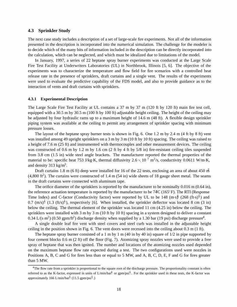
The Large Scale Fire Test Facility at UL contains a 37 m by 37 m (120 ft by 120 ft) main fire test cell,equipped with a 30.5 m by 30.5 m (100 ft by 100 ft) adjustable height ceiling. The height of the ceiling maybe adjusted by four hydraulic rams up to a maximum height of 14.6 m (48 ft). A flexible design sprinklerpiping system was available at the ceiling to permit any arrangement of sprinkler spacing with minimumpressure losses.
The layout of the heptane spray burner tests is shown in Fig. 6. One 1.2 m by 2.4 m (4 ft by 8 ft) ventwas installed among 49 upright sprinklers on a 3 m by 3 m (10 ft by 10 ft) spacing. The ceiling was raised toa height of 7.6 m (25 ft) and instrumented with thermocouples and other measurement devices. The ceilingwas constructed of 0.6 m by 1.2 m by 1.6 cm (2 ft by 4 ft by 5/8 in) fire-resistant ceiling tiles suspendedfrom 3.8 cm (1.5 in) wide steel angle brackets. The manufacturer reported the thermal properties of thematerial to be: specific heat 753 J/kg�K, thermal diffusivity 2:6� 10�7 m2/s, conductivity 0.0611 W/m�K,and density 313 kg/m3.
Draft curtains 1.8 m (6 ft) deep were installed for 16 of the 22 tests, enclosing an area of about 450 m2
(4,800 ft2). The curtains were constructed of 1.4 m (54 in) wide sheets of 18 gauge sheet metal. The seamsin the draft curtains were connected with aluminum tape.
The orifice diameter of the sprinklers is reported by the manufacturer to be nominally 0.016 m (0.64 in),the reference actuation temperature is reported by the manufacturer to be 74�C (165�F). The RTI (ResponseTime Index) and C-factor (Conductivity factor) were reported by UL to be 148 (m�s)
12 (268 (ft�s)
12 ) and
0.7 (m/s)12 (1.3 (ft/s)
12 ), respectively [6]. When installed, the sprinkler deflector was located 8 cm (3 in)
below the ceiling. The thermal element of the sprinkler was located 11 cm (4.25 in) below the ceiling. Thesprinklers were installed with 3 m by 3 m (10 ft by 10 ft) spacing in a system designed to deliver a constant0.34 L/(s�m2) (0.50 gpm/ft2) discharge density when supplied by a 1.30 bar (19 psi) discharge pressure4.
A single double leaf fire vent with steel covers and steel curb was installed in the adjustable heightceiling in the position shown in Fig. 6. The vent doors were recessed into the ceiling about 0.3 m (1 ft).
The heptane spray burner consisted of a 1 m by 1 m (40 in by 40 in) square of 1/2 in pipe supported byfour cement blocks 0.6 m (2 ft) off the floor (Fig. 7). Atomizing spray nozzles were used to provide a freespray of heptane that was then ignited. The number and locations of the atomizing nozzles used dependedon the maximum heptane flow rate expected during a test. The two configurations used were nozzles inPositions A, B, C and G for fires less than or equal to 5 MW, and A, B, C, D, E, F and G for fires greaterthan 5 MW.
4The flow rate from a sprinkler is proportional to the square root of the discharge pressure. The proportionality constant is oftenreferred to as the K-factor, expressed in units of L/min/bar
12 or gpm/psi
12 . For the sprinkler used in these tests, the K-factor was
approximately 166 L/min/bar12 (11.5 gpm/psi
12 .)
18

North Wall
Adjustable Height Ceiling
Draft Curtains
?
6
36.6 m
?
6
30.5 m
?
6
21.7 m
� -20.4 m� -6.4 m � -3.7 m
6
?
7.9 m
6 0.9 m
?
60.6 m
-� �
0.9 m
3.0 m
A
B
C
D
r
r
r
r
r
r
r
r
r
r
r
r
r
r
r
r
r
r
r
r
r
r
r
r
r
r
r
r
r
r
r
r
r
r
r
r
r
r
r
r
r
r
r
r
r
r
r
r
r
98 91 84 81 78 75 72
99 92 85 82 79 76 73
100 93 86 83 80 77 74
101 94 87 62 58 54 50
102 95 88 63 59 55 51
103 96 89 64 60 56 52
104 97 90 65 61 57 53
68
69
70
67 66
71
ppppppp 43
444546474849
Figure 6: Plan view of heptane spray burner configuration, Series I. The sprinklers are indicated bythe solid circles and are spaced 3 m (10 ft) apart. The number beside each sprinkler location indicatesthe channel number of the nearest thermocouple. The vent dimensions are 1.2 m by 2.4 m (4 ft by 8 ft).The boxed letters A, B, C and D indicate burner positions. Corresponding to each burner position isa vertical array of thermocouples. Thermocouples 1–9 hang 7, 22, 36, 50, 64, 78, 92, 106 and 120 infrom the ceiling, respectively, above Position A. Thermocouples 10 and 11 are positioned above andbelow the ceiling tile directly above Position B, followed by 12–20 that hang at the same levels belowthe ceiling as 1–9. The same pattern is followed at Positions C and D, with thermocouples 21–31 at Cand 32–42 at D.
19

Fuel Supply�
� -1 m� -.35 m � -.30 m
?
6
1 m
?
6.35 m
?
6.30 m
u u
u
u
u u
u
u
AH
G
F
DE
B
C
Figure 7: Plan view of heptane spray burner.
For all but one of the tests, the total heat release rate from the fire was ramped following the t-squaredcurve
Q = Q0
� tτ
�2(1)
where Q0 = 10 MW and τ = 75 s. The fire growth curve was followed until a specified fire size was reachedor the first sprinkler activated. After either of these events, the fire size was maintained at that level untilconditions reached roughly a steady state, i.e. the temperatures recorded near the ceilings remained steadyand no more sprinkler activations occurred.
Temperature measurements were recorded at 104 locations. Sheathed thermocouples were positionedto measure (i) temperatures near the ceiling, (ii) temperatures of the ceiling jet, and (iii) temperatures nearthe vent. The thermocouples numbered 50–65 were positioned near the sprinklers, 10 cm (4 in) belowthe ceiling. These were intended to measure near-sprinkler gas temperatures as well as to detect sprinkleractivation when wetted. Thermocouples 66–104 were placed 5 cm (2 in) below the ceiling. Thermocouples43–49 ran down the centerline of the vent at the level of the ceiling, and were spaced 0.3 m (1 ft) apart.Thermocouples 1–42 were mounted on arrays hanging above each fire location. The positions are noted inthe caption to Fig. 6.
4.3.2 Simulation Parameters
Figure 8 contains the parameters that define the numerical simulation of one of the tests described above.The first decision made by the modeler is the size of the computational domain. Because the test facility is alarge rectangular volume, it would seem natural to model the entire space. However, this is costly because theCPU time expended on the calculation is directly proportional to the number of grid cells used. Instead, thevolume beneath the adjustable height ceiling that is bounded by the draft curtains, plus a small volume abovethe ceiling to accommodate the flow of smoke through the vent, is chosen as the computational domain. Theorigin of the coordinate system is the southwest corner of the curtained area at the floor. Because the fireis in the northeast corner of the curtained area, the grid cells are clustered here by means of the coordinatetransformations in the x and y directions.
The fire is represented by a solid obstruction, 0.5 m high, with its top designated as a burner. Given theresolution of the underlying grid, it is not possible to model the burner as a set of spray nozzles mounted to asquare ring of pipe. Instead, the whole burner is idealized as a solid surface out of the top of which burning
20

&HEAD CHID=’heptane’,TITLE=’Heptane Burner Test’ /&GRID IBAR=50,JBAR=52,KBAR=32 /&PDIM XBAR=20.45,YBAR=21.69,ZBAR=9.00 /&TRNX CC= 2.454,PC= 8.000 /&TRNY CC= 3.337,PC= 8.000 /&TIME DT=0.10,TWFIN=300. /&MISC TMPA=14.,DATABASE=’database’ /&PART NPSAM=5 /&SURF ID=’BURNER’,HRRPUA=4400.,TAU_Q=-50.,TBO=0.6 /&SURF ID=’CEILING’,ALPHA=2.6E-7,DELTA=0.016,KS=0.0611 /&OBST XB=14.38,15.60,13.11,15.54, 7.92, 8.50, SURF_ID=’CEILING’ /&OBST XB= 0.00,14.38,13.11,15.54, 7.62, 8.50, SURF_ID=’CEILING’ /&OBST XB=15.60,20.45,13.11,15.54, 7.62, 8.50, SURF_ID=’CEILING’ /&OBST XB= 0.00,20.45, 0.00,13.11, 7.62, 8.50, SURF_ID=’CEILING’ /&OBST XB= 0.00,20.45,15.54,21.69, 7.62, 8.50 /&OBST XB=14.50,15.50,16.87,17.87, 0.00, 0.50 /&VENT XB=14.50,15.50,16.87,17.87, 0.50, 0.50, SURF_ID=’BURNER’ /&VENT XB= 0.00, 0.00, 0.00,21.69, 0.00, 5.79, SURF_ID=’OPEN’ /&VENT XB=20.45,20.45, 0.00,21.69, 0.00, 5.79, SURF_ID=’OPEN’ /&VENT XB= 0.00,20.45, 0.00, 0.00, 0.00, 5.79, SURF_ID=’OPEN’ /&VENT XB= 0.00,20.45,21.69,21.69, 0.00, 5.79, SURF_ID=’OPEN’ /&PIPE PRESSURE=1.30 /&SPRK XYZ= 1.270, 0.610, 7.462,MAKE=’K-11’ /&SPRK XYZ= 4.318, 0.610, 7.462,MAKE=’K-11’ /&SPRK XYZ= 7.366, 0.610, 7.462,MAKE=’K-11’ /
.
.
.&THCP QUANTITY=’TEMPERATURE’, XYZ=15.051,14.160, 7.386 /&THCP QUANTITY=’TEMPERATURE’, XYZ=15.051,14.160, 7.005 /&THCP QUANTITY=’TEMPERATURE’, XYZ=15.051,14.160, 6.650 /
.
.
.
Figure 8: Input file for sprinkler scenario.
thermal elements are ejected. The area of the burner is 1 m2 and the heat release rate per unit area is 4,400kW/m2. The heat release rate is ramped up to 4,400 kW in 50 s following a t-squared growth curve, andafter 50 s the heat release rate remains at 4,400 kW. It should be noted that by default 35% of the energyis radiated away. No surfaces have been designated to absorb this radiation, thus the energy is “lost” as faras the calculation is concerned. The burn-out time of the thermal elements is set to be 0.6 s based on flameheight correlations. See Ref. [1] for more details.
The other obstructions listed define the adjustable height ceiling and the vent within it. Note in this casethat the vent is passive, but it is not at the boundary of the computational domain. This vent is merely apassageway from one part of the domain to another, thus it is defined by prescribing 5 obstructions. Fourof these obstructions are sections of the ceiling, the fifth is the vent itself. The sections of the ceiling areassigned thermally-thick boundary conditions representative of the insulating tiles. The fifth obstruction iscontrolled by a heat detector that can activate automatically or manually, much like in the actual experiments.The heat detector is located where the vent’s thermal link would be located, and it is assigned properties thatbest reflect those of the link.
The sprinklers are designated as ’K-11’, and the listing in the DATABASE is given in Fig. 9. The C-Factor is 0.7 (m/s)
12 , K-Factor 166 L/min/bar
12 , RTI 148 (ms)
12 , orifice diameter 0.016 m, median droplet di-
21

ameter 0.0013 m, operating pressure 1.30 bar, and activation temperature 74�C. The parameters SPRAY ANGLE 0and SPRAY ANGLE 1 indicate the angles from the vertical through which the droplets will be ejected. Notethat the PIPE PRESSURE in the input file indicates the pressure at which the sprinklers in the simulationshould operate. The parameter SPR OP PRESS in the DATABASE file indicates the pressure at which thesprinkler was tested and the properties obtained.
&SMOD SNAME = ’K-11’CFAC = 0.7KFAC = 166.RTI = 148.ODIAM = 0.016SPRAY_ANGLE_0 = 30.SPRAY_ANGLE_1 = 80.DM = 0.0013SPR_OP_PRESS = 1.30TMPLA = 74. /
Figure 9: Parameters for K-11 sprinkler.
Finally, the positions of the 104 thermocouples are listed in at the end of the input file. The temperaturesrecorded at these locations can then be compared with the measurements made during the actual test.
4.3.3 Results
A comparison of the temperatures at the nearest 16 sprinklers is shown in Fig. 10. Activation of a sprinkleris indicated by a rapid decrease in temperature. The thermocouple temperatures will decrease to ambientin the experiment, but the temperature predicted by the calculation will not because it continues to recordthe gas temperature. In the experiment, 11 sprinklers activated, whereas in the simulation, 12 activated.Channel 51 shows the temperatures near the sprinkler that did not activate in the experiment, but did in thesimulation.
A complete description of all the experiments and the calculations is included in Ref. [5]. The resultsshown here are intended to demonstrate the capability of FDS for a fire test in which the heat release rateis well characterized. Even though sprinklers are activating, the fire size is not decreasing because a sprayburner is being used. The cooling of the hot gases by the water droplets is being accounted for in thecalculation, but not suppression.
22

Figure 10: Near-sprinkler temperature measurement (dashed lines) compared to numerical simula-tion (solid lines) for nearest 16 sprinklers.
23

4.4 Large Outdoor Fires
In this section the near field hazard associated with flame radiation is studied. The scenario is a fire burningthe contents of an oil storage tank adjacent to several neighboring tanks [7]. The heat release generatedby a fire on this scale can reach several gigawatts if the entire pool surface is exposed and burning. Suchfires interact strongly with the local topography (both natural and man made), and the vertical distributionof wind and temperature in the atmosphere.
The radiation is emitted as a prescribed fraction of the chemical energy released in each Lagrangianelement used to describe the fire energy input. This fraction, typically in the thirty to thirty five percentrange, is the same as that used previously in earlier studies of enclosure fires [8]. The difference is that afraction of the fuel mass in each burning element is converted to soot. The soot thus introduced is allowedto absorb radiant energy. The radiant energy flux arriving on the target surface is calculated by summing theexact solution to the radiative transport equation for a discrete set of point emitters with a prescribed energyrelease. The effect of the absorption on the plume hydrodynamics is accounted for by using the analyticalsolution to calculate the divergence of the flux from the same random sample of Lagrangian elements usedto compute the surface heat transfer. A check for self-consistency is made by noting that the fraction of thecombustion energy released arriving as radiation on the target surfaces is close to that estimated from crudeoil experiments [9].
The fire is burning the oil spilled from a tank into a containment trench surrounding it. Each of the tanksshown sits partially depressed in a spill containment trench surrounded by a sloping embankment of height9 m. The wind speed profile and thermal stratification of the atmosphere are selected to be representative ofthe atmospheric boundary layer under stable conditions prevalent in northern winter climates. A numericalgrid consisting of 128 by 128 by 128 cells was used to span a cubic domain 768 m on a side. The cell sizewas 6 m by 6 m in the horizontal directions and ranged from 3 m near the ground to 12 m at the top of thecube in the vertical. The diameter of each tank was 84 m, the height 27 m. These tanks were incorporatedinto the calculation by “blocking” cells. Because boundary layers are not resolvable (except the planetaryboundary layer) at this grid resolution, there is little penalty in assuming that the tank walls are not smooth,but rather are saw-toothed. The geometry of each tank and its associated “trench” were modeled on the oilstorage facility of the Japan National Oil Corporation at Tomakomai. No attempt was made to simulate theentire facility, which contains over 80 tanks.
A stratified wind profile of the form
u(z) = u0
�zz0
�p
(2)
was imposed as a boundary condition. The wind speed u0 at the height of the tanks (z0 = 27 m) was10 m/s. The exponent p, a function of the surface roughness, was 0.15. The temperature of the ambientatmosphere was assumed to be uniform with height (20�C), although any resolvable temperature profile canbe input. The fire was assumed to be engulfing the entire top of the tank, burning with a heat release rate of1,500 kW/m2, for a total of 8.2 GW. The fraction of the chemical heat release rate converted into thermalradiation and emitted from the thermal elements was assumed to be 35%. However, much of the emittedradiant energy is re-absorbed by the surrounding smoke. The ramifications of this smoke shielding can berealized by computing the radiative flux to the surrounding tanks. For the case of the burning tank top in a10 m/s wind (Fig. 11), the radiative flux to the side of the downwind tank was 1.6 kW/m2. A test calculationwas performed in which no thermal radiation was absorbed by the smoke. For this case, the flux to thedownwind tank was 9.0 kW/m2. Thus the effective radiative fraction is (1:6=9:0)�35% or about 6%. Thisestimate is consistent with the measurements of Koseki [9].
24

Figure 11: Instantaneous snapshot of a tank fire simulation with the wind speed 6 m/s at the tops of the tanks and the fire in the trench.
25

&HEAD CHID=’tankfarm’,TITLE=’Japanese Oil Storage Tank Farm’ /&GRID IBAR=128,JBAR=128,KBAR=48 /&PDIM XBAR0= 0.,XBAR=768.,YBAR0=0.,YBAR=768.,ZBAR=288. /&TRNZ IDERIV=1,CC=0.,PC=0.5 /&TRNZ IDERIV=2,CC=0.,PC=0.0 /&TIME DT=0.5,TWFIN=120. /&MISC TMPA=20.,DT0DZ=0.,SURF_DEFAULT=’EARTH’,RADIATIVE_ABSORPTION=.TRUE. /&PART DTPAR=.20 /&SURF ID=’EARTH’,RADIATION=.TRUE. /&SURF ID=’WIND’,VEL=-10.,PROFILE=’ATMOSPHERIC’,Z0=27.,PLE=0.15,TMPWAL=20. /&SURF ID=’FIRE’,HRRPUA=1500.,TBO=2.1,RADIATIVE_FRACTION=0.35,
RADIATION=.TRUE.,SMOKE_YIELD=0.12,DELTAH=40000. /&OBST XB= 0.,138., 0.,768., 0., 9. /&OBST XB=138.,144., 0.,768., 0., 6. /&OBST XB=144.,150., 0.,768., 0., 3. /
.
.&OBST XB=174.,180.,372.,396., 0., 27.,SURF_IDS=’FIRE’,’EARTH’,’EARTH’ /&OBST XB=180.,186.,360.,408., 0., 27.,SURF_IDS=’FIRE’,’EARTH’,’EARTH’ /&OBST XB=186.,192.,354.,414., 0., 27.,SURF_IDS=’FIRE’,’EARTH’,’EARTH’ /
.
.&VENT XB= 0., 0., 0.,768., 9.,768.,SURF_ID=’WIND’ /&VENT CB=’YBAR’ ,SURF_ID=’OPEN’ /&VENT CB=’YBAR0’,SURF_ID=’OPEN’ /&VENT CB=’XBAR’ ,SURF_ID=’OPEN’ /&VENT CB=’ZBAR’ ,SURF_ID=’OPEN’ /&SLCF XB= 0.,768.,384.,384., 0.,768.,QUANTITY=’TEMPERATURE’ /&BNDF QUANTITY=’RADIATIVE_FLUX’ /&PL3D DTSAM=60. /
Figure 12: Input file for oil tankfarm fire scenario.
26

4.5 Rack Storage Fire
The most challenging application of the Fire Dynamics Simulator has been racked storage fire tests with aboxed commodity. These calculations involve fire growth in a complicated fuel geometry, sprinkler acti-vation, and suppression by water. Of these, suppression is the most difficult phenomenon to characterize.The fuel for the tests was the FMRC Standard Plastic commodity, which consists of polystyrene cups incorrugated paper cartons. Details of the full scale experiments are given in Ref. [5]. Details of the smallscale burns are given in Ref. [10]. The input file for a simulation of one of the tests is given in Fig. 14.The physical domain of the calculation is taken to be the volume underneath a curtained area of the testfacility. Sprinklers are spaced every 3 m (10 ft) near the ceiling. The pallet loads of fuel are represented assolid obstructions whose tops, sides and bottoms have different thermal and burning properties. Ignition isachieved by creating a small fire at the floor between two pallet loads of fuel. The heat release rate and timeduration of the ignition fire are based on calorimeter measurements of the cotton roll ignitors used at UL.
The simulation of rack storage commodity fires is still a subject of active research at NIST. Since thepublication of Ref. [5], experiments have been performed to improve the suppression model [10], but thesprinkler characterization has not been improved. The drop size distribution and spray pattern from thesprinkler used in these tests has yet to be measured.
27

Figure 13: Geometry of rack storage fire simulation.
28

&HEAD CHID=’plastic’,TITLE=’Group A Plastic Commodity Test’ /&GRID IBAR=64,JBAR=62,KBAR=40 /&PDIM XBAR=21.34,YBAR=23.16,ZBAR=8.23 /&TRNX CC= 2.00,PC= 4.09 /&TRNX CC=17.67,PC=14.04 /&TRNY CC= 9.05,PC=10.96 /&TRNY CC=16.65,PC=15.41 /&TIME DT=0.10,TWFIN=300. /&MISC TMPA=18.,DATABASE=’database’ /&PL3D DTSAM=60. /&PART AGE=30.,NSPSAM=7,NPSAM=7,DTPAR=0.025 /&SURF ID=’IGNITION’,HRRPUA=3000.,VEL=-0.40,TBO=0.3,RAMP_Q=’IGN’ /&RAMP ID=’IGN’,T= 0.0,F=0.0 /&RAMP ID=’IGN’,T=10.0,F=1.0 /&RAMP ID=’IGN’,T=40.0,F=0.0 /&OBST XB= 4.09, 5.15, 8.52, 9.58, .00, 1.23,
SURF_IDS=’PLASTIC A TOP’,’PLASTIC A’,’PALLET’ /&OBST XB= 5.36, 6.42, 8.52, 9.58, .00, 1.23,
SURF_IDS=’PLASTIC A TOP’,’PLASTIC A’,’PALLET’ /..
&VENT XB= 8.96, 9.17,12.45,12.65, 0.00, 0.00,SURF_ID=’IGNITION’ /&VENT XB= 0.00, 0.00, 0.00,23.16, 0.00, 6.40,SURF_ID=’OPEN’ /&VENT XB=21.34,21.34, 0.00,23.16, 0.00, 6.40,SURF_ID=’OPEN’ /&VENT XB= 0.00,21.34, 0.00, 0.00, 0.00, 6.40,SURF_ID=’OPEN’ /&VENT XB= 0.00,21.34,23.16,23.16, 0.00, 6.40,SURF_ID=’OPEN’ /&PIPE PRESSURE=1.3 /&SPRK XYZ= 1.524, .305, 8.154,MAKE=’K-11’ /&SPRK XYZ= 4.572, .305, 8.154,MAKE=’K-11’ /&SPRK XYZ= 7.620, .305, 8.154,MAKE=’K-11’ /
.
.&THCP XYZ= 1.524, .305, 8.154,QUANTITY=’TEMPERATURE’ /&THCP XYZ= 4.572, .305, 8.154,QUANTITY=’TEMPERATURE’ /
.
.
Figure 14: Input data file for full scale rack storage fire simulation.
29

5 Glossary of Input Parameters
The first step in performing a calculation is to generate a text input file that will provide the program with allof the necessary information to describe the scenario under consideration. The most important inputs deter-mine the physical size of the overall rectangular domain, the grid dimensions, and the additional geometricalfeatures. Next, the energy sources must be prescribed and other boundary conditions. Finally, there are anumber of parameters that customize the output files to capture the most important flow quantities. Inputdata is prescribed by writing a small file that uses the NAMELIST formatted records. Each line of the filebegins with the character & followed immediately by the name of the NAMELIST group (HEAD, GRID,VENT, etc.), followed by a list of the input parameters corresponding to that group. Each list is terminatedwith a slash. Note that the parameters listed are only those that the user desires to be changed from thedefault.
Table 5: Namelist Groups.
Name Purpose
HEAD Header information, job IDGRID Grid dimensionsPDIM Physical dimensionsTRNX Coordinate transformation parameters for x directionTRNY Coordinate transformation parameters for y directionTRNZ Coordinate transformation parameters for z directionTIME Time duration of simulation and initial time stepMISC Miscellaneous or global inputsSPEC Additional speciesREAC Single step reaction rate parameters (DNS only)SURF Surface or boundary conditionsOBST Solid obstacles or obstructionsVENT Planar vents or wall patchesSPRK Sprinkler informationHEAT Heat detector informationRAMP Ramp-up functions for fire or other quantitiesPART Thermal element variables and outputPL3D PLOT3D output data setsTHCP Point measurement outputSLCF 1, 2 or 3 dimensional output data setsBNDF Boundary or surface quantity output data sets
5.1 TheHEAD Namelist Group
The namelist group HEAD contains two parameters. CHID is character string of 30 characters or less usedto tag output files with a given character string. If, for example, CHID=’casename’, it is convenient toname the input data file casename.dataso that the input file can be associated with the output files. Noperiods are allowed in CHID because the output files are tagged with suffixes that are meaningful to certaincomputer operating systems. TITLE is a character string of 60 characters or less that describes the problem.
30

s
(XBAR0,YBAR0,ZBAR0) x
z
-
����*
y
6
������
�����
������
�����
������
�����
� -XBAR-XBAR0
�����
����*
YBAR-YBAR0
?
6
ZBAR-ZBAR0
Figure 15: Domain geometry.
5.2 TheGRID Namelist Group
The namelist group GRID contains the dimensions of the computational grid. The grid consists of IBARcells in the x direction, JBAR cells in the y direction, and KBAR cells in the z direction. Usually, the zdirection is assumed to be the vertical direction. The longer horizontal dimension should be taken as thex-direction. Also, because an important part of the calculation uses a Poisson solver based on Fast FourierTransforms (FFTs), the dimensions of the grid should each be of the form 2l 3m 5n, where l, m and n areintegers. For example, 64 = 26, 72 = 2332 and 108 = 2233 are good grid dimensions. However, 37, 99 and109 are not.
5.3 ThePDIM Namelist Group
PDIM is the name of the group of parameters defining the size of the physical domain. The coordinatesystem spanned by these dimensions conforms to the right hand rule (See Fig. 15). The physical domain is asingle right parallelepiped, i.e. a box. The origin of the domain is the point (XBAR0,YBAR0,ZBAR0), andthe opposite corner of the domain is at the point (XBAR,YBAR,ZBAR). By default, XBAR0, YBAR0,ZBAR0 are zero, in which case the physical dimensions of the domain are given as XBAR, YBAR and ZBARin units of meters. Unless otherwise directed, the domain will be subdivided uniformly to form a grid ofIBAR by JBAR by KBAR cells. If it is desired that the grid cells not be uniform in size, then the namelistgroups TRNX, TRNY and/or TRNZ may be used to alter the uniform gridding.
5.4 TheTRNX, TRNY and/or TRNZ Namelist Groups
By default the grid cells that fill the computational domain are uniform in size. However, it is possible tospecify that the cells be non-uniform in one or two of the three coordinate directions. For a given coordinatedirection, x, y or z, a function can be prescribed that maps the uniformly-spaced computational grid to anon-uniformly spaced physical grid. Take the x direction as an example. A function x = f (ξ) will map the
31
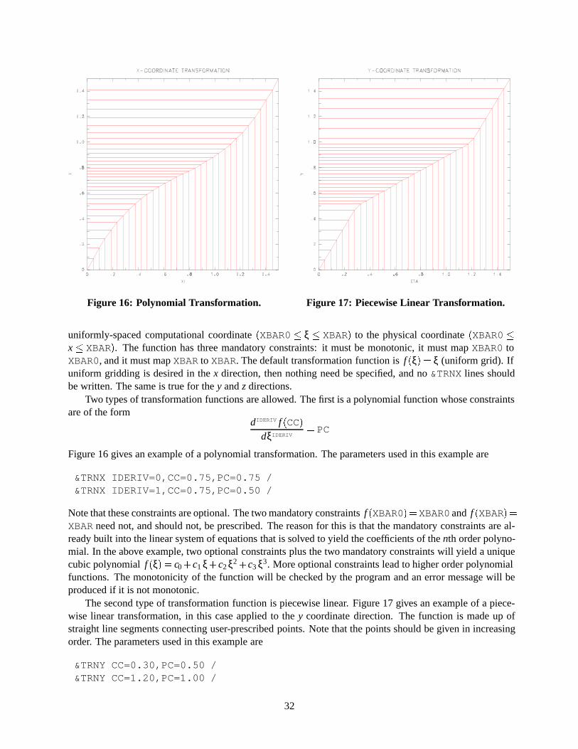
Figure 16: Polynomial Transformation. Figure 17: Piecewise Linear Transformation.
uniformly-spaced computational coordinate (XBAR0 � ξ � XBAR) to the physical coordinate (XBAR0 �x � XBAR). The function has three mandatory constraints: it must be monotonic, it must map XBAR0 toXBAR0, and it must map XBAR to XBAR. The default transformation function is f (ξ) = ξ (uniform grid). Ifuniform gridding is desired in the x direction, then nothing need be specified, and no &TRNX lines shouldbe written. The same is true for the y and z directions.
Two types of transformation functions are allowed. The first is a polynomial function whose constraintsare of the form
dIDERIV f (CC)dξIDERIV
= PC
Figure 16 gives an example of a polynomial transformation. The parameters used in this example are
&TRNX IDERIV=0,CC=0.75,PC=0.75 /&TRNX IDERIV=1,CC=0.75,PC=0.50 /
Note that these constraints are optional. The two mandatory constraints f (XBAR0)=XBAR0 and f (XBAR)=XBAR need not, and should not, be prescribed. The reason for this is that the mandatory constraints are al-ready built into the linear system of equations that is solved to yield the coefficients of the nth order polyno-mial. In the above example, two optional constraints plus the two mandatory constraints will yield a uniquecubic polynomial f (ξ) = c0+c1 ξ+c2 ξ2+c3 ξ3. More optional constraints lead to higher order polynomialfunctions. The monotonicity of the function will be checked by the program and an error message will beproduced if it is not monotonic.
The second type of transformation function is piecewise linear. Figure 17 gives an example of a piece-wise linear transformation, in this case applied to the y coordinate direction. The function is made up ofstraight line segments connecting user-prescribed points. Note that the points should be given in increasingorder. The parameters used in this example are
&TRNY CC=0.30,PC=0.50 /&TRNY CC=1.20,PC=1.00 /
32

Note that for a piecewise linear transformation, the parameter IDERIV should not be used. Indeed, thepresence of IDERIV signals a polynomial rather than a piecewise linear transformation.
The vertical and horizontal lines on Figs. 16 and 17 indicate how the uniformly spaced computationalgrid on the horizontal axis is transformed into a non-uniformly spaced physical grid on the vertical axis. Theslope of the transformation function indicates the degree to which the computational cells will be stretched(slope greater than 1) or shrunk (slope less than 1). Note that shrinking cells in one region will necessarilylead to stretching cells elsewhere. When one or two coordinate directions are transformed, the aspect ratioof the grid cells in the 3D mesh will vary. To be on the safe side, transformations that alter the aspect ratioof cells beyond 2 or 3 should be avoided. Keep in mind that the large eddy simulation technique is basedon the assumption that the numerical grid should be fine enough to allow the formation of eddies that areresponsible for the mixing. In general, eddy formation is limited by the largest dimension of a grid cell,thus shrinking the grid in one or two directions may not necessarily lead to a better simulation if the thirddimension is large. Also note that transformations, in general, reduce the efficiency of the computation, withtwo coordinate transformations impairing efficiency more than a transformation in one coordinate direction.
5.5 TheTIME Namelist Group
TIME is the name of a group of parameters defining the time duration of the simulation and the initial timestep used to advance the solution of the discretized equations.
DT Starting time step size in seconds. This input can be determined roughly by dividing the size of a gridcell by the characteristic velocity of the flow. During the calculation, the time step will be adjusted sothat the CFL condition is satisfied. (Default 0.1 s)
TWFIN Time when finished in seconds. This tells how long the simulation is to be run. (Default 1.0 s)
5.6 TheMISC Namelist Group
MISC is the namelist group of miscellaneous input parameters. Only one MISC line should be entered inthe data file. The MISC parameters vary in scope and degree of importance. The most important param-eter in this category is the one that determines whether a Large Eddy Simulation (LES) calculation is tobe performed, or whether a Direct Numerical Simulation (DNS) is to be performed. By default, an LEScalculation will be performed. If a DNS calculation is desired, enter DNS=.TRUE. on the MISC line. Also,certain global defaults are established via this group. If more than one species is being included in the cal-culation, the MISC line is used to establish what the predominant (or background) species is. By default,this BACKGROUND SPECIES is ’AIR’, but often in combustion-related calculations, a more appropriateBACKGROUND SPECIES is ’NITROGEN’. The properties of these gases are known to the program, sothe user need not say anything more about them. However, if the desired BACKGROUND SPECIES is notincluded in Table 6, the user must provide the molecular weight MW for a gas or DENSITY for a liquid inunits of g/mol or kg/m3, respectively. If the user is performing a DNS calculation, the VISCOSITY (kg/m/s)and THERMAL CONDUCTIVITY (W/m/K) must also be provided for an unlisted species.
Some other parameters prescribed on the MISC line are:
DATABASE A character string indicating the name of a file that contains information about particular sprin-klers, surface materials, or other auxiliary data. This need only be specified if sprinklers or surfacematerials other than those specified by the user are called for.
SURF DEFAULT Character string indicating which of the listed SURF IDs is to be considered the default.The default is ’INERT’.
33

DTCORE The interval of time (s) between “restart” dumps. Every DTCORE s, all of the flow variables willbe saved in a file called casename.restart. To restart a job from this point, the file casename.restartshould be designated by the parameter RESTART FILE which needs to be added to the MISC lineof the data file controlling the continued job. It’s a good idea to rename the continued job so thatthe output files from the original job are not overwritten. (Default for DTCORE is infinity, meaningno restart dumps will be made unless specified, or when the user gracefully stops a job by creating adummy file called casename.stop.)
RESTART FILE Character string containing the name of the “restart” file if the job is to be a continuationof a previously performed calculation.
TMPA Ambient temperature in degrees Celsius. (Default 15�C)
GVEC Gravity vector in units of m/s2. (Default GVEC=0.,0.,-9.81)
ISOTHERMAL Logical expression indicating that the calculation does not involve any change in temper-ature, thus reducing the number of equations that must be solved, simplifying those that are, andreducing the computation time. (Default .FALSE.)
RADIATIVE ABSORPTION Logical expression indicating whether the smoke should be allowed to absorbthermal radiation. This is a time-consuming option. (Default .FALSE.)
RMAX Maximum distance for which a single ray trace will be computed for thermal radiation. This is auseful parameter if the fire is located in one room and the user wants to prevent wasted ray traces toother rooms during the calculation of radiative flux. (Default unlimited)
DT0DZ Lapse rate of the atmosphere in units of�C/m. This need only be set for outdoor calculations wherethe height of the domain is tens or hundreds of meters. (Default -g/cp �-0.0097 �C/m)
NFRAMES Default number of output dumps per calculation. Thermocouple data, slice data, particle data,and boundary data will be saved every TWFIN/NFRAMES unless otherwise specified with DTSAM onthe THCP, SLCF, PART, and BNDF namelist lines. (Default 500)
PR Prandtl number used in an LES calculation to relate the viscosity to the thermal conductivity, k= cpµ=Pr.(Default 0.2)
SC Schmidt number used in an LES calculation to relate the viscosity to the material diffusivity, ρD= µ=Sc.(Default 0.2)
CSMAG Smagorinsky constant (LES only). (Default 0.14)
DTWALL Time step for solid phase temperature updates and radiation calculation. (Default 0.1 s)
5.7 TheSPEC and REAC Namelist Groups
By default, only one gas species is included in a calculation. For most applications this gas is air. Tochange the default gas species, specify BACKGROUND SPECIES under the MISC namelist group. Forsimulations involving mixtures of gas species, SPEC is the namelist group that is used to specify eachadditional species. Do not enter a SPEC line for the background species. Each SPEC line should include thename of the species (ID) and its ambient (initial) mass fraction, MASS FRACTION 0. Several gases thatcan be included in a calculation are listed in Table 6. The physical properties of these gases are known andneed not be specified. However, if a desired gas species is not included in Table 6, its molecular weight MW
34

Table 6: Optional Gas Species [11]
Species Mol. Wgt. σ k=ε(g/mol) (A) (K)
AIR 29 3.711 78.6CARBON DIOXIDE 44 3.941 195.2CARBON MONOXIDE 28 3.690 91.7HELIUM 4 2.551 10.22METHANE 16 3.758 148.6NITROGEN 28 3.798 71.4OXYGEN 32 3.467 106.7PROPANE 44 5.118 237.1WATER VAPOR 18 2.641 809.1
for a gas or DENSITY for a liquid must be specified in units of g/mol or kg/m3, respectively. In addition, ifa DNS calculation is being performed, either the Lennard-Jones potential parameters σ (SIGMALJ) and ε=k(EPSILONKLJ) should be specified; or the VISCOSITY (kg/m/s), THERMAL CONDUCTIVITY (W/m/K),and DIFFUSION COEFFICIENT (m2/s) between the given species and the background species should bespecified.
If the listed species is reacting, its stoichiometric coefficient, NU, needs to be specified. Include a minussign if the species is being consumed in the combustion process. The stoichiometric coefficient is requiredonly if fuel and oxygen are reacting. Note that the background species is not allowed to participate in thereaction. Often NITROGEN is a good candidate for the background species when oxygen is being consumed.
In an LES calculation, if oxygen is prescribed as an optional species, then automatically oxygen willbe consumed by the fire at a rate of 13,100 kJ/kg. If the oxygen mass fraction within a given grid cellfalls below OXBOMF, a parameter prescribed on the same line as the oxygen, no combustion will take placewithin that cell, and the thermal elements will not burn until they enter a cell with an oxygen mass fractionabove OXBOMF.
In a DNS calculation, if a reaction is to take place between a given fuel and oxygen, the REAC namelistgroup is used to designate the fuel and the reaction rate parameters. If one of the species is designated asoxygen, but no species is designated as fuel, then thermal elements will be used to introduce heat into thecalculation and oxygen will be depleted according to the overall heat release rate of the elements.
FUEL Character string indicating which of the listed optional gas species is the fuel.
BOF Pre-exponential factor in one-step chemical reaction in units of cm3/mole/s.
EACT Activation energy for one-step chemical reaction in units of kcal/mole.
XNO Exponent for oxygen concentration in one-step chemical reaction.
XNF Exponent for fuel concentration in one-step chemical reaction.
DELTAH The effective heat of combustion for one-step chemical reaction in units of kJ/kg. (Default 40,000kJ/kg)
35

5.8 TheSURF Namelist Group
SURF is the namelist group that defines boundary conditions for all solid surfaces or openings within orbounding the flow domain. The physical coordinates of obstructions or vents are listed in the OBST andVENT namelist groups below. Boundary conditions for the obstructions and vents are prescribed by refer-encing the appropriate SURF line(s) whose parameters will be described presently.
The default boundary condition for all solid surfaces is that of an adiabatic, inert wall. If only thisboundary condition is needed, there is no need to add any SURF lines to the input file. If additional boundaryconditions are desired, they are to be listed one boundary condition at a time. Each SURF line consists ofan identification string ID to enable reference to it by an obstruction or vent. Thus, on each OBST andVENT line, the character string SURF ID indicates the ID of the SURF line containing the desired boundarycondition parameters. These parameters describe the thermal properties and burning characteristics of asolid, or the velocity and composition of the gas entering or leaving through a vent.
5.8.1 Thermal Boundary Conditions
There are four types of thermal boundary conditions: adiabatic, constant temperature, thermally-thick orthermally-thin. For a given boundary condition (i.e. for the same SURF line), choose only one of these.The simplest condition, adiabatic, is the default, and nothing need be set to obtain it. Adiabatic walls donot absorb heat from the gas. For a wall of fixed temperature, set TMPWAL to be the wall temperature inunits of �C. For thermally-thick walls, prescribe the thermal diffusivity ALPHA (m2/s), the thermal con-ductivity KS (W/m�K), and the thickness DELTA (m) of the wall. Setting these parameters will direct thecode to perform a one-dimensional heat transfer calculation within the wall. For thermally-thin walls, pre-scribe C DELTA RHO, the product of the specific heat (kJ/kg-K), density (kg/m3), and thickness (m) of thewall/surface. A thermally-thin wall is assumed to be the same temperature throughout its width. By default,if a surface is designated as thermally-thin or thermally-thick, the radiative flux from the fire to that surfacewill be calculated. This calculation is relatively expensive, thus if the radiative flux to that surface is deemedinsignificant, the radiation calculation can be turned off by setting RADIATION=.FALSE.. The convec-tive heat transfer to the surface will still be calculated. Also note that adiabatic or constant temperaturesurfaces can include a radiation calculation by setting RADIATION=.TRUE.. Doing this will not affectthe calculation, but will provide the radiative fluxes to these surfaces for output purposes.
Another way to save on the cost of calculating radiation heat transfer to surfaces is to set a parametercalled RMAX on the MISC line. RMAX is the maximum distance in meters that a ray will be traced whencomputing radiative fluxes. Setting RMAX to, say 3, will restrict ray traces to less than 3 m, thus objectsmore than 3 m away from the fire will not feel the effect of the radiation. This parameter is useful whenperforming large, multi-room calculations because it restricts the unnecessary tracing of rays to objects farfrom the source of radiant energy.
5.8.2 Velocity Boundary Condition
Velocity boundary conditions effect both the normal and tangential components of the velocity vector atboundaries. The tangential velocity boundary condition can be no-slip, free-slip or something in between (asimple law of the wall). For no-slip, set VBC to -1. For free-slip, set VBC to 1. Numbers in between -1 and1 can represent partial slip conditions, which may be appropriate for simulations involving large grid cells.(Default VBC is 0.5 for LES, -1.0 for DNS)
The normal component of velocity is controlled by the parameter VEL. If VEL is negative, the flow isentering the computational domain. If VEL is positive, the flow is exiting the domain. By default the velocityprofile at the surface is a top hat, but the parameter PROFILE can yield other profiles. PROFILE=’PARABOLIC’
36
produces a parabolic profile, and PROFILE=’ATMOSPHERIC’ produces a typical atmospheric wind pro-file of the form u = u0(z=z0)
p. If an atmospheric profile is prescribed, also prescribe Z0 for z0 and PLE forp. VEL specifies the reference velocity u0.
Sometimes it is desired that a given volume flux through a vent be prescribed rather than a velocity.If this is the case then VOLUME FLUX can be prescribed instead of VEL. The units are m3/s. If the flowis into the computational domain, VOLUME FLUX should be a negative number. Note that either VEL orVOLUME FLUX should be prescribed, not both. The choice depends on whether an exact velocity is desiredat a given vent, or whether the given volume flux is desired. Keep in mind that the dimensions of the ventthat are prescribed will usually change because the prescribed vent dimensions are sometimes altered so thatthe vent edges line up with grid cells. Also note that a SURF group with a VOLUME FLUX prescribed shouldonly be associated with a VENT, not an OBST.
5.8.3 Prescription of a Fire (LES only)
A fire must originate at a solid surface; thus prescribing a fire is equivalent to setting some additionalboundary conditions. A fire is basically modeled as the ejection of thermal elements (discretized parcelsof burning fuel) from the surface at a given velocity. This velocity is usually small, but it is necessary to“push” the burning elements away from the surface. When a fire is prescribed, thermal elements are ejectedfrom the appropriate solid surface. If no fire is prescribed, no thermal elements will be ejected unlessPARTICLES=.TRUE. is included on the SURF line. Non-burning particles may be colored by speci-fying PARTICLE COLOR=’RED’, ’BLUE’, ’BLACK’, ’YELLOW’, ’GREEN’, ’MAGENTA’,’WHITE’ or ’CYAN’
Following is a list of parameters that are prescribed on a SURF line to designate a fire.
TMPIGN The temperature (C) at which the wall begins burning. This is only set if the wall is thermally-thickor thermally-thin, that is, if the wall is assumed to be heating up. Heat fluxes to the walls are both con-vective and radiative, with the radiative energy determined from the value of RADIATIVE FRACTION.If TMPIGN is set, a heat release rate per unit area HRRPUA should also be given. (Default: TMPIGNis 5000�C, i.e. no burning will occur)
HRRPUA Heat release rate per unit area in units of kW/m2. This can be prescribed with either adiabatic,thermally-thin or thermally-thick boundary conditions. The time of ignition can be explicitly specifiedwith TIGN or it can be determined automatically by the calculation in the case of thermally-thin orthick walls. (Default 0.)
TBO Burn-out time of the thermal elements that represent the fire. (Default 0.25 s)
RADIATIVE FRACTION The fraction of the energy from combustion converted into thermal radiation.The convective heat release rate can be monitored in the output file or in the file casenamehrr.csv.The energy converted to radiation will not play a role in the simulation unless certain surfaces arespecified as either thermally-thick or thermally-thin, in which case they are allowed to heat up and theradiative flux to these surfaces will be calculated. (Default 0.35)
DELTAH The effective heat of combustion of the fuel. (Default 20,000 kJ/kg)
SMOKE YIELD The fraction of the fuel mass that is converted into particulate matter. This parameter mustbe set if it is desired that the smoke absorb thermal radiation (RADIATIVE ABSORPTION=.TRUE.on the MISC line). Also, if the quantity SMOKE DENSITY is desired as output in either a PLOT3Dfile, slice file or thermocouple file. (Default 0.)
37

NPPC Number of thermal elements introduced into the flow field per active surface cell every DTPARseconds. Increasing this will not change the heat release rate, but in some cases it can improve theanimation of the fire. (Default 1)
HRPUV Heat Release Per Unit Volume. The energy contained within a cubic meter of fuel in units of kJ/m3.This parameter need only be set if the fuel is to disappear once it has burned out. No default value –it is assumed the fuel will remain burning unless this parameter is specified.
E COEFFICIENT An array of five parameters that characterize suppression of the fire by water. The localheat release rate of the fuel is expressed in the form [10]
q00f (t) = q00f ;0(t)�
e�R
k1 dt + k2(t� t0)�
(3)
Here q00f ;0(t) is the heat release rate per unit area of the fuel when no water is applied and k1 and k2 arefunctions of the local water mass per unit area, m00w, expressed in units of kg/m2.
k1 = a1 m00
w s�1 (4)
k2 = a2 m00
w+b2 s�1 (5)
The parameter a1 is given by E COEFFICIENT(1) for the first E COEFFICIENT(3) s of burning,after which it is given by E COEFFICIENT(2). The parameter a2 is given by E COEFFICIENT(4)and b2 is given by E COEFFICIENT(5).
POROSITY The fraction of water that does not cascade down the side of the fuel package, either becauseof absorption or because it is trapped within the interior of the fuel. (Default 0.)
5.8.4 Species Boundary Conditions
There are three types of boundary conditions for the Nth species listed with a SPEC namelist group. If asimple no-flux condition is desired at a solid wall, do not set anything. If the mass fraction of the Nth speciesis to be some value at a forced flow boundary, set MASS FRACTION(N) equal to the desired mass fraction.Use TAU MF(N), an array of NSPEC ramp-up times for the NSPEC species, to control the ramp-ups (seebelow). The mass fraction of species N at the surface is given by
YN(t) =YN(0)+ f (t)(YN �YN(0))
where YN(0) is the ambient mass fraction of species N (MASS FRACTION 0 in the Nth SPEC namelistgroup is used to prescribe YN(0)), YN is the desired mass fraction to which the function f (t) is ramping(MASS FRACTION(N) specified in the SURF line is used to prescribe YN). The function f (t) is either atanh, t2, or user defined function. For a user defined function, indicate the name of the ramp function withRAMP MF(N), a character string (see Time Dependent Boundary Conditions below). If a particular massflux of the Nth species is desired, set MASS FLUX(N) instead of MASS FRACTION(N). The mass flux isin units of kg/m2/s. Note that the thermal boundary conditions and velocity must also be set in addition tothe mass flux.
If the surface is burning, one can specify the yield of a given species with the parameter YIELD(N).This parameter indicates the amount of species N produced as a fraction of the fuel mass loss rate. Forexample, a CO yield of 0.01 means that 0.01 kg of CO are formed for every 1 kg of fuel consumed. IfYIELD(N) is specified then the following conditions need to be met: There should be a species N declaredwith a SPEC card. Neither MASS FRACTION(N) nor MASS FLUX(N) should be specified because theproduction rate of species N is now tied to the heat release rate HRRPUA via the heat of combustion DELTAH,
38

both of which need to be specified. Neither TAU MF(N) nor RAMP MF(N) should be specified because thetime history of species N production is now linked to that of the HRRPUAwhose time history is governed byTAU Q or RAMP Q.
5.8.5 Time Dependent Boundary Conditions
At the start of any calculation, the temperature is ambient everywhere, the flow velocity is zero everywhere,nothing is burning, the mass fractions of all species are uniform. When the calculation starts temperatures,velocities, burning rates, etc., are ramped-up from their starting values because nothing can happen instanta-neously. By default, everything is ramped-up to their prescribed values in roughly 1 s. However, the user cancontrol the rate at which things turn on, or turn off, by specifying time histories for the boundary conditionsthat are listed on a given SURF line. The above boundary conditions can be made time-dependent usingeither prescribed functions or user-defined functions. The parameters TAU Q, TAU V, and TAU MF(N) in-dicate that certain quantities are to ramp up to their prescribed values in TAU seconds and remain there.TAU Q is the characteristic ramp-up time of the heat release rate per unit area HRRPUA or wall temper-ature TMPWAL. TAU V is the ramp-up time of the normal velocity at a surface VEL or the volume fluxVOLUME FLUX. TAU MF(N) is the ramp-up time of the mass fraction MASS FRACTION(N) or mass fluxMASS FLUX(N) of the Nth species. If TAU Q is positive, then the heat release rate ramps up like tanh(t=τ).If negative, then the HRR ramps up like (t=τ)2. If the fire ramps-up like following a t2 curve, it will remainconstant after TAU Q seconds. These rules apply to TAU V and TAU MF(N) as well. The default value forall TAUs is 1 s. If something other than a tanh or t2 ramp up is desired, then a user-defined burning historymust be input. To do this, set RAMP Q, RAMP V, or RAMP MF(N) equal to a character string designatingthe ramp function to use for that particular surface type, then somewhere in the input file generate lines ofthe form:
&RAMP ID=’rampname1’,T= 0.0,F=0.0 /&RAMP ID=’rampname1’,T= 5.0,F=0.5 /&RAMP ID=’rampname1’,T=10.0,F=0.7 /
.
.
.&RAMP ID=’rampname2’,T= 0.0,F=0.0 /&RAMP ID=’rampname2’,T=10.0,F=0.3 /&RAMP ID=’rampname2’,T=20.0,F=0.8 /
.
.
.
Here, T is the time, and F indicates the fraction of the heat release rate, wall temperature, velocity, massfraction, etc., to apply. Linear interpolation is used to fill in intermediate time points. Be sure that theprescribed function starts at T=0., the ignition time. Note that the TAUs and the RAMPs are mutuallyexclusive. For a given surface quantity, both cannot be prescribed.
5.9 TheOBST Namelist Group
OBST is the namelist group listing information about obstructions. Each OBST line contains the coordinatesof a rectangular solid within the flow domain. This solid is defined by two points (x1,y1,z1) and (x2,y2,z2)that are entered on the OBST line in terms of the sextuplet XB=X1,X2,Y1,Y2,Z1,Z2. In addition tothe coordinates, the boundary conditions for the obstruction can be specified with the parameter SURF ID,
39
which designates which SURF group to apply at the surface of the obstruction. If the obstruction has differentboundary conditions for its top, sides and bottom, then instead of prescribing only one boundary conditionwith SURF ID, use SURF IDS, an array of three character strings specifying the boundary condition IDsfor the top, sides and bottom of the obstruction, respectively. If the default boundary condition is desired,then SURF ID(S) need not be set. However, if at least one of the surface conditions for an obstruction isthe inert default, it can be referred to as ’INERT’.
One other useful parameter in this group is IDEVICE. This parameter is the index of the HEAT detectorwhich, when activated, will cause the given obstruction to disappear. The removal of an obstruction can beused to model the opening of a door or vent that connects one part of the domain to another. If a door or avent to the outside is desired, then IDEVICE can be associated with a VENT. More on VENTs and HEATdetectors below.
Blocks may be colored by specifying BLOCK COLOR=’RED’, ’BLUE’, ’BLACK’, ’YELLOW’,’GREEN’, ’MAGENTA’, ’WHITE’ or ’CYAN’
5.10 TheVENT Namelist Group
Whereas the OBST group is used to prescribe obstructions within the computational domain, the VENTgroup is used to prescribe planes adjacent to obstructions or external walls. The vents are chosen in asimilar manner to the obstructions, with the sextuple XB denoting a plane abutting a solid surface. Twoof the six coordinates must be the same, denoting a plane as opposed to a solid. An easy way to specifyan entire external wall is to replace XB with CB, a character string whose value is one of the following:’XBAR’, ’XBAR0’, ’YBAR’, ’YBAR0’, ’ZBAR’ or ’ZBAR0’ denoting the planes x = XBAR, x =XBAR0, y = YBAR, y = YBAR0, z = ZBAR or z = ZBAR0, respectively. Like an obstruction, the boundarycondition index of a vent is specified with SURF ID, indicating which of the listed SURF lines to apply. Ifthe default boundary condition is desired, then SURF ID need not be set. If the vent is a passive openingto the outside, then SURF ID should be set equal to ’OPEN’. If the vent is a symmetry plane, SURF IDshould be set equal to ’MIRROR’. Note that only vents aligned with external walls can be designated asOPEN or MIRROR. Entire walls may be removed by making the vent as large as the wall and designatingit as a passive opening. If a passive opening is specified for one or more vents, there can be no build-up ofpressure in the enclosure, in other words, the enclosure vents to an infinite reservoir.
As with OBSTructions, passive vents to the outside can be opened according to the activation of a HEATdetector. To do this, set IDEVICE equal to the index of the HEAT detector that will control the vent. TheSURF ID for this vent must be ’OPEN’.
Vents may be colored by specifying VENT COLOR=’RED’, ’BLUE’, ’BLACK’, ’YELLOW’,’GREEN’, ’MAGENTA’, ’WHITE’ or ’CYAN’
5.11 TheSPRK Namelist Group
SPRK specifies sprinklers. The physical coordinates of the sprinkler are given by a triplet of real numbersXYZ. The make of the sprinkler is given by a character string MAKE. Choices of sprinklers can be foundin the database file indicated by the parameter DATABASE in the MISC namelist group. The sprinklerwill activate automatically based on its thermal properties listed in DATABASE. The user has the option ofmanually activating the sprinkler by setting TACT in seconds on the SPRK line itself. To control the flowrate from a sprinkler, the user must set the pressure in the sprinkler piping with a separate line of the form
&PIPE PRESSURE=1.30 /
Each sprinkler in the database has a K-factor associated with it, so the flow rate will be given by
mw = Kp
p
40

where mw is the flow rate in L/min, K the K-factor in L/min/(bar)12 and p the gauge pressure in bar5
Sprinkler properties listed in the DATABASE file are
RTI Response Time Index of the sprinkler in units ofp
m � s. (Default 165.)
CFAC C-Factor of sprinkler in units ofp
m/s. (Default 0.)
KFAC K-Factor of sprinkler in units of L/min/bar12 . (Default 166)
ODIAM Orifice diameter of sprinkler in meters. (Default 0.016)
DM Median drop diameter in meters. (Default 0.001)
TMPLA Link activation temperature (C). (Default 74�C)
SPRAY ANGLE 0, SPRAY ANGLE 1 Angles in degrees from the vertical centerline axis between whichthe sprinkler droplets are ejected. Straight down corresponds to 0 degrees, horizontal is 90 degrees.(Default 10.,80.)
SPR OP PRESS Sprinkler operating pressure in units of bar. This is the pressure at which the sprinkler wastested at. (Default 1.30)
5.12 TheHEAT Namelist Group
HEAT specifies heat detectors. Like a sprinkler, the physical coordinates of the heat detector are given by atriplet of real numbers XYZ. The make of the heat detector is given by a character string MAKE. Choices ofsprinklers can be found in the database indicated by the parameter DATABASE in the MISC namelist group.Automatic thermal activation can be overridden with TACT. Properties of a heat detector that is listed in theDATABASE are
RTI Response Time Index of heat detector in units ofp
m � s. (Default 165.)
CFAC C-Factor of heat detector in units ofp
m/s. (Default 0.)
TMPLA Link activation temperature (C). (Default 74�C)
5.13 ThePART Namelist Group
PART is the namelist group that is used to specify how the thermal elements and sprinkler droplets are to beincluded in the calculation. Some of the parameters contained in this group are purely for output purposesand will not affect the calculation.
DTPAR Time increment between thermal element insertions in seconds. If more particles are desired, lowerthe input value of this parameter. This parameter does affect the calculation because it controls howoften thermal elements are being ejected from burning surfaces. Ideally, DTPAR should be about thesame as the time step size. (Default 0.05 s)
DTSPAR Time increment between sprinkler droplet insertions (s). Like DTPAR, DTSPAR does have aneffect on the calculation. (Default 0.05 s)
51 bar is equivalent to 14.5 psi, 1 gpm is equivalent to 3.785 L/min, 1 gpm/psi12 is equivalent to 14.41 L/min/bar
12 .
41

NSPINS Number of sprinkler droplets inserted every DTSPAR seconds per active sprinkler. The numberof water droplets introduced into the flow domain per sprinkler per second is NSPINS/DTSPAR.(Default NSPINS is 50)
The following parameters have no effect on the calculation but rather control the number of particles dumpedto the output files and the quantity with which to color the particles in the animation.
AGE Lifetime of a thermal element in seconds. If AGE is prescribed, the thermal elements will be removedfrom the calculation AGE s following their insertion. This parameter can be used to reduce the numberof burned out elements that need to be tracked and save on CPU time. (Default unlimited)
DTSAM Incremental time between thermal element (and sprinkler droplet) data dumps in seconds. Thesedumps add to a file called casename.partwhich can be used to produce an animation of the flow field.(Default TWFIN/NFRAMES)
NPSAM Sampling factor for the thermal element output file casename.part. This parameter can be used toreduce the size of the particle dump file used to animate the simulation. (Default 1)
NPPS Number of particles per set. The maximum number of thermal elements that can be dumped into thefile casename.partevery DTSAM seconds. (Default 100000)
QUANTITY A character string indicating which scalar quantity should be used to color the particles whenviewed as an animation. Choices are listed in Table 7.
NIP Number of Initial Particles. This parameter allows the user to seed the domain with particles at thestart of the simulation. (Default 0)
Table 7: Quantities used to color thermal elements.Quantity Description Symbol Units
TEMPERATURE gas temperature T CHRRPUV Heat Release Rate Per Unit Volume q000 kW/m3
[SPECIES] species mass fraction Y
5.14 TheTHCP Namelist Group
THCP lists thermocouple or other point measurements. Each line in this group consists of the coordinatesof the point at which the measurement is to be recorded, XYZ, and a quantity to record, QUANTITY. Theseare either quantities associated with a given grid cell (see Table 8) or a surface cell (see Table 9). Whenprescribing a surface cell quantity, be sure to position the coordinates within a solid wall. It is not alwaysobvious where the wall is since the grid does not always align with the input obstruction locations. The codewill spit out an error message if a surface quantity is not embedded in a wall. If the orientation of the probeis not obvious, specify IOR appropriately. If the probe is facing in the positive x direction IOR=1, negativex direction IOR=-1, positive y IOR=2, negative IOR=-2, positive z IOR=3, and negative z IOR=-3.Also, the sampling rate of the measurements is specified with the parameter DTSAM. Since the samplingrate is the same for all point measurements, it need only be specified once. The default value for DTSAM isTWFIN/NFRAMES s. The time to start and stop recording can be controlled with the parameters TSTARTand TSTOP whose defaults are 0 and TWFIN. The thermocouples can be labeled with the character stringLABEL for easier identification in the output file.
42

Table 8: Gas Phase Output Quantities forTHCP, SLCF or PL3D.
Quantity Description Symbol Units Comments
DENSITY density ρ kg/m3
U-MOMENTUM momentum component ρu kg/m2/s line or planeV-MOMENTUM momentum component ρv kg/m2/s line or planeW-MOMENTUM momentum component ρw kg/m2/s line or planeTEMPERATURE gas temperature T CU-VELOCITY velocity component u m/sV-VELOCITY velocity component v m/sW-VELOCITY velocity component w m/sVELOCITY velocity
pu2+ v2+w2 m/s
PRESSURE perturbation pressure p PaHRRPUV Heat Release Rate Per Unit Volume q000 kW/m3
DYNAMIC VISCOSITY dynamic viscosity µ kg/m/sKINEMATIC VISCOSITY kinematic viscosity µ=ρ m2/sDIVERGENCE divergence ∇ �u s�1
WMPUV Water Mass Per Unit Volume m000
w kg/m3
[SPECIES] species mass fraction Y[SPECIES] VF species volume fraction X[SPECIES] FLUX X species mass flux ρuY kg/m2/s line or plane[SPECIES] FLUX Y species mass flux ρvY kg/m2/s line or plane[SPECIES] FLUX Z species mass flux ρwY kg/m2/s line or planeSMOKE DENSITY smoke density µg/m3
DROPLET FLUX vertical droplet flux kg/m2/s planar SLCF onlyDROPLET DIAMETER average sprinkler droplet diameter m planar SLCF only
5.15 ThePL3D Namelist Group
PL3D is the namelist group that defines how often and what quantities are to be dumped into files ofPLOT3D format. At most one PL3D line should be listed in the input file.
DTSAM Incremental time between PLOT3D data dumps in seconds. (Default TWFIN/5)
TSTART Time to start dumping PLOT3D data.
TSTOP Time to stop dumping PLOT3D data.
QUANTITIES An array of five quantities that are to be in included in the PLOT3D data sets. See Table 8for a list of output quantities. (Default: ’TEMPERATURE’, ’U-VELOCITY’, ’V-VELOCITY’,’W-VELOCITY’, ’HRRPUV’)
5.16 TheSLCF Namelist Group
The SLCF (“slice file”) namelist group allows the user to record various gas phase quantities (Table 8) atmore than a single point. A “slice” refers to a subset of the whole domain. It can be a line, plane, orvolume, depending on the values of XB. The sextuple XB indicates the boundaries of the region for whichvalues of QUANTITY are to be recorded every DTSAM s starting at TSTART s and ending at TSTOP s. XBis prescribed as in the OBST or VENT groups, with the possibility that 0, 2, or 4 out of the 6 values bethe same to indicate a volume, plane or line, respectively. Slice file information is recorded in files labeled
43
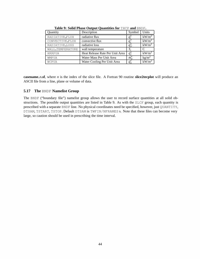
Table 9: Solid Phase Output Quantities forTHCP and BNDF.Quantity Description Symbol Units
RADIATIVE FLUX radiative flux q00r kW/m2
CONVECTIVE FLUX convective flux q00c kW/m2
RADIATIVE LOSS radiative loss q00rr kW/m2
WALL TEMPERATURE wall temperature Ts CHRRPUA Heat Release Rate Per Unit Area q00f kW/m2
WMPUA Water Mass Per Unit Area m00
w kg/m2
WCPUA Water Cooling Per Unit Area q00w kW/m2
casenamen.sf, where n is the index of the slice file. A Fortran 90 routine slice2tecplotwill produce anASCII file from a line, plane or volume of data.
5.17 TheBNDF Namelist Group
The BNDF (“boundary file”) namelist group allows the user to record surface quantities at all solid ob-structions. The possible output quantities are listed in Table 9. As with the SLCF group, each quantity isprescribed with a separate BNDF line. No physical coordinates need be specified, however, just QUANTITY,DTSAM, TSTART, TSTOP. Default DTSAM is TWFIN/NFRAMES s. Note that these files can become verylarge, so caution should be used in prescribing the time interval.
44

6 Output File Formats
The output from the code consists of the file casename.out, plus various data files that will be describedbelow. Most of these output files are written out by the routine dump.f, and can easily be modified toaccommodate various plotting packages.
6.1 Diagnostic Output
A file called casename.outis created if the program is run in the background and the file casename.outisprescribed as standard out. The file casename.outconsists of a list of the input parameters, and an account-ing of various important quantities, including CPU usage. Typically, diagnostic information is printed outevery 100 time steps
.
.
100 CPU/step: 3.870 s, Total CPU: 6.59 minTime step: 0.02885 s, Total time: 3.33 sMax divergence: 0.63E+01 at ( 30, 32, 1)Max CFL number: 0.98E+00 at ( 30, 33, 14)Number of Thermal Elements: 65Convective Heat Release Rate: 59.821 kW
200 CPU/step: 3.909 s, Total CPU: 13.10 minTime step: 0.02786 s, Total time: 6.08 sMax divergence: 0.98E+01 at ( 30, 32, 1)Max CFL number: 0.85E+00 at ( 30, 33, 14)Number of Thermal Elements: 211Convective Heat Release Rate: 108.130 kW
.
.
The number on the left indicates the number of the time step. The quantity CPU/step is the amount ofCPU time required to complete a time step; Total CPU is the amount of CPU time elapsed since the startof the run; Time step is the time step size of the simulation; Total time is the time of the simulation;Max divergence is the maximum value of the function ∇ �u and is used as a diagnostic when the flowis incompressible (i.e. no heating); and CFL number is the maximum value of the CFL number. The lasttwo values are self-explanatory.
Following the completion of a successful run, a summary of the CPU usage per subroutine is listed.This is useful in determining where most of the computational effort is being put.
6.2 PLOT3D Data
Presently, field data is dumped every DTSAM seconds in a format used by the graphics package PLOT3D.The PLOT3D data sets are single precision (32 bit reals), whole and unformatted. Note that there is blank-ing, that is, blocked out data points are not plotted. The grid data is written out to a file called casename.xyz
WRITE(LU13) IBAR+1,JBAR+1,KBAR+1WRITE(LU13) (((X(I),I=0,IBAR),J=0,JBAR),K=0,KBAR),
45

. (((Y(J),I=0,IBAR),J=0,JBAR),K=0,KBAR),
. (((Z(K),I=0,IBAR),J=0,JBAR),K=0,KBAR),
. (((IBLK(I,J,K),I=0,IBAR),J=0,JBAR),K=0,KBAR)
where X, Y and Z are the coordinates of the cell corners, and IBLK is an indicator of whether or not the cellis blocked. If the point (X,Y,Z) is completely embedded within a solid region, then IBLK is 0. Otherwise,IBLK is 1. The flow variables are written to a file called casename**** **.q , where the stars indicate atime at which the data is dumped. The file is written with the lines
WRITE(LU14) IBAR+1,JBAR+1,KBAR+1WRITE(LU14) ZERO,ZERO,ZERO,ZEROWRITE(LU14) ((((QQ(I,J,K,N),I=0,IBAR),J=0,JBAR),K=0,KBAR),N=1,5)
The five channels N=1,5 are by default the temperature (C), the u, v and w components of the velocity(m/s), and the heat release rate per unit volume (kW/m3). Alternate variables can be specified with the inputparameter QUANTITIES under the PL3D namelist group. Note that the data is interpolated at cell corners,thus the dimensions of the PLOT3D data sets are one larger than the dimensions of the computational grid.
The package smokeviewcan display the PLOT3D data. In addition, the PLOT3D data sets can be readinto whatever graphics routine the user has available, as long as the format of the data is specified. Thisparticular format is very convenient, and recognized by a number of graphics packages, including AVS,IRIS Explorer and Tecplot 6.
6.3 Thermocouple Data
Temperature (or other scalar quantity) data at discrete points specified in the input file under the NAMELISTgroup THCP is output in comma delimited format in a file called casenametc.csv. The format of the file isas follows
NTC, LABEL(1) , LABEL(2) , ... , LABEL(NTC)
TIME, QUANTITY(1), QUANTITY(2), ... , QUANTITY(NTC)s , UNITS(1) , UNITS(2) , ... , UNITS(NTC)T , TC(1) , TC(2) , ... , TC(NTC)
.
.
.
where NTC is the number of thermocouples, LABEL is a user-defined tag, QUANTITY is the physical quan-tity represented, UNITS the units, T the time of the dump, and TC(I) the value at the Ith thermocouple, inthe order that they are listed in the input file. The files can be imported into Microsoft Excel or other spreadsheet programs.
6.4 Sprinkler Data
If sprinklers are prescribed in the calculation, then a file called casenamespk.csvwill be generated. Thefile lists the temperature of each sprinkler link.
6With the exception of smokeview, the graphics packages referred to in this document are not included with the source code,but are commercially available.
46

NSPRTIME,TEMP ,TEMP ,...,TEMPs ,C ,C ,...,CT ,TL(1),TL(2),...,TL(NSPR)
.
.
.
where NSPR is the number of sprinklers, T is the time of the dump, TL(I) is the link temperature of theIth sprinkler. The data will be ordered the same way as the sprinklers are listed in the input file.
6.5 Heat Release Rate
The convective heat release rate of the fire is reported in the comma delimited file casenamehrr.csv. Thefile consists of two columns of numbers, the first column containing the time in seconds, the second containsthe convective heat release rate in units of kW.
6.6 Slice Files
The slice files defined under the NAMELIST group SLCF are named casenamen.sf (n=01,02...), and arewritten out unformatted, unless otherwise directed. These files are written out from dump.f with the follow-ing lines:
WRITE(LUSF) QUANTITYWRITE(LUSF) SHORT_NAMEWRITE(LUSF) UNITSWRITE(LUSF) I1,I2,J1,J2,K1,K2WRITE(LUSF) TIMEWRITE(LUSF) (((QQ(I,J,K),I=11,I2),J=J1,J2),K=K1,K2)
.
.
.WRITE(LUSF) TIMEWRITE(LUSF) (((QQ(I,J,K),I=11,I2),J=J1,J2),K=K1,K2)
QUANTITY,SHORT NAME and UNITS are character strings of length 30. The sextuple (I1,I2,J1,J2,K1,K2)denotes the bounding grid cell nodes. The sextuple indices correspond to grid cell nodes, or corners, thusthe entire grid would be represented by the sextuple (0,IBAR,0,JBAR,0,KBAR).
There is a short Fortran 90 program provided, called slice2tecplot.f, that can convert slice files intoASCII files that can be read into a variety of graphics packages. The program combines multiple slice filescorresponding to the same “slice” of the computational domain, time-averages the data, and writes the valuesinto one file, consisting of a line of numbers for each node. Each line contains the physical coordinates ofthe node, and the time-averaged quantities corresponding to that node. In particular, the package Tecplotwill read this file and produces contour, streamline and/or vector plots.
6.7 Boundary Files
The boundary files defined under the NAMELIST group BNDF are named casenamen.bf (n=01,02...), andare written out unformatted. These files are written out from dump.f with the following lines:
47

WRITE(LUBF) QUANTITYWRITE(LUBF) SHORT_NAMEWRITE(LUBF) UNITSWRITE(LUBF) NPATCHWRITE(LUBF) I1,I2,J1,J2,K1,K2WRITE(LUBF) I1,I2,J1,J2,K1,K2
.
.
.WRITE(LUBF) TIMEWRITE(LUBF) (((QQ(I,J,K),I=11,I2),J=J1,J2),K=K1,K2)WRITE(LUBF) (((QQ(I,J,K),I=11,I2),J=J1,J2),K=K1,K2)
.
.
.WRITE(LUBF) TIMEWRITE(LUBF) (((QQ(I,J,K),I=11,I2),J=J1,J2),K=K1,K2)WRITE(LUBF) (((QQ(I,J,K),I=11,I2),J=J1,J2),K=K1,K2)
.
.
.
QUANTITY, SHORT NAME and UNITS are character strings of length 30. NPATCH is the number of planes(or “patches”) that make up the solid boundaries plus the external walls. The sextuple (I1,I2,J1,J2,K1,K2)defines the cell nodes of each patch. The user does not prescribe these. Note that the data is planar, thus onepair of nodes will be the same.
Presently, smokeviewis the only program available to view the boundary files. See details above.
6.8 Particle Data
The thermal elements and sprinkler droplets are animated using a file called casename.part. It contains theparticle positions. There is a one line header followed by particle locations dumped every DTSAM seconds.The structure of the data file is given in the file dump.f by a subroutine called PDMP3D.
WRITE(LU10) ARX,ARY,DTSAM,IPART,NPPSWRITE(LU10) IBAR,JBAR,KBARWRITE(LU10) (X(I),I=0,IBAR),(Y(J),J=0,JBAR),(Z(K),K=0,KBAR)WRITE(LU10) NBDO N=1,NBWRITE(LU10) IB1(N),IB2(N),JB1(N),JB2(N),KB1(N),KB2(N),1END DOWRITE(LU10) NVDO N=1,NVWRITE(LU10) IV1(N),IV2(N),JV1(N),JV2(N),KV1(N),KV2(N),2END DOWRITE(LU10) NSPRDO N=1,NSPRWRITE(LU10) XSP0(N),YSP0(N),ZSP0(N)END DO
48

where ARX=ZBAR/XBAR and ARY=ZBAR/YBAR are the aspect ratios of the overall domain, IPART isthe index of the scalar quantity associated with the particles, NPPS is the maximum number of particles perframe, IB1, IB2, etc. are the indices of blocked grid cells, IV1, IV2, etc. indicate vent cell nodes, andXSP0, YSP0, ZSP0 are the coordinates of the sprinklers. The arrays X(I), Y(J), Z(K) containthe coordinates of the grid. Every DTSAM seconds the coordinates of the thermal elements and sprinklerdroplets are dumped
WRITE(LU10) TIME,NP,NN,(ISPR(N),N=1,NSPR)WRITE(LU10) (XP(I),I=1,NP),. (YP(I),I=1,NP),. (ZP(I),I=1,NP),. (BP(I),I=1,NP)IF (NASPR.GT.0) THENWRITE(LU10) NSPWRITE(LU10) (XSP(I),I=1,NSP),(YSP(I),I=1,NSP),(ZSP(I),I=1,NSP)ENDIF
where NP is the number of thermal elements, NN is a dummy integer kept for compatibility reasons, ISPRdenotes whether the sprinkler has activated, NSPR is the number of sprinklers, XP, YP, ZP are the coor-dinates of the element, BP is a the quantity referenced by IPART, NASPR is the number of active sprinklers,NSP is the number of sprinkler droplets, and XSP, YSP, ZSP are the droplet coordinates.
49

7 Conclusion
The equations and numerical algorithm described in this document form the core of an evolving fire model.As research into specific fire-related phenomena continues, the relevant parts of the model can be improved.Because the model was originally designed to analyze industrial scale fires, it can be used reliably when thefire size is specified and the building is relatively large in relation to the fire. In these cases, the model pre-dicts flow velocities and temperatures to an accuracy of 10 to 20% compared to experimental measurements.Currently, research is focussed on improving both the gas phase and solid phase descriptions of combustionin the model so that simulations involving fire growth and suppression, especially in residential sized rooms,can be improved.
Any user of the numerical model must be aware of the assumptions and approximations being employed.There are two issues for any potential user to consider before embarking on calculations. First, for both realand simulated fires, the growth of the fire is very sensitive to the thermal properties of the surroundingmaterials. Second, even if all the material properties are known, the physical phenomena of interest may notbe simulated due to limitations in the model algorithms or numerical grid. Except for those few materialsthat have been studied to date at NIST, the user must supply the thermal properties of the materials, and thenvalidate the performance of the model with experiments to ensure that the model has the necessary physicsincluded. Only then can the model be expected to predict the outcome of fire scenarios that are similar tothose that have actually been tested.
50

References
[1] K.B. McGrattan, H.R. Baum, R.G. Rehm, A. Hamins, and G.P. Forney. Fire Dynamics Simulator,Technical Reference Guide. Technical Report NISTIR 6467, National Institute of Standards and Tech-nology, Gaithersburg, Maryland, January 2000.
[2] Mason Woo, Jackie Neider, and Tom Davis. OpenGL Programming Guide. Addison-Wesley Devel-opers Press, Reading, Massachussets, 1996.
[3] Mark J. Kilgard. OpenGL Programming for the X Window System. Addison-Wesley Developers Press,Reading, Massachussets, 1996.
[4] H.R. Baum and B.J. McCaffrey. Fire Induced Flow Field – Theory and Experiment. In Fire Safety Sci-ence – Proceedings of the Second International Symposium, pages 129–148. International Associationfor Fire Safety Science, 1989.
[5] K.B. McGrattan, A. Hamins, and D. Stroup. Sprinkler, Smoke & Heat Vent, Draft Curtain Interaction— Large Scale Experiments and Model Development. Technical Report NISTIR 6196-1, NationalInstitute of Standards and Technology, Gaithersburg, Maryland, September 1998.
[6] D.T. Sheppard and D.R. Steppan. Sprinkler, Heat & Smoke Vent, Draft Curtain Project – Phase 1Scoping Tests. Technical report, Underwriters Laboratories, Inc., Northbrook, Illinois, May 1997.
[7] H.R. Baum and K.B. McGrattan. Simulation of Large Industrial Outdoor Fires. In Fire Safety Science– Proceedings of the Sixth International Symposium. International Association for Fire Safety Science,1999.
[8] K.B. McGrattan, H.R. Baum, and R.G. Rehm. Large Eddy Simulations of Smoke Movement. FireSafety Journal, 30:161–178, 1998.
[9] H. Koseki and T. Yumoto. Air Entrainment and Thermal Radiation from Heptane Pool Fires. FireTechnology, 24, February 1988.
[10] A. Hamins and K.B. McGrattan. Reduced-Scale Experiments to Characterize the Suppression of RackStorage Commodity Fires. Technical Report NIST Internal Report (NISTIR 6439), National Instituteof Standards and Technology, Gaithersburg, Maryland 20899, 1999.
[11] R.C. Reid, J.M. Prausnitz, and B.E. Poling. Properties of Gases and Liquids. McGraw-Hill, Inc., NewYork, 4th edition, 1987.
51