finite size effects near the onset of the oscillatory
TRANSCRIPT

Finite size effects near the onset of the oscillatory instability
Carlos Martel and José M Vega ETSI Aeronáuticos, Universidad Politécnica de Madrid, 28040-Madrid, Spain
Abstract. A system of two complex Ginzburg-Landau equations is considered that applies at the onset of the oscillatory instability in spatial domains whose size is large (but finite) in one direction; the dependent variables are the slowly modulated complex amplitudes of two counterpropagating wavetrains. In order to obtain a well posed problem, four boundary conditions must be imposed at the boundaries. Two of them were already known, and the other two are first derived in this paper. In the generic case when the group velocity is of order unity, the resulting problem has terms that are not of the same order of magnitude. This fact allows us to consider two distinguished limits and to derive two associated (simpler) sub-models, that are briefly discussed. Our results predict quite a rich variety of complex dynamics that is due to both the modulational instability and finite size effects.
AMS classification scheme numbers: 35B25, 35B32, 35Q35, 76E30
1. Introduction
The oscillatory instability is one of the few generic universal ways [1] in which nearly uniform steady states of physical systems in large spatial domains (i.e. large compared with the appropriate inherent characteristic length) may lose stability. Experimental results in fluid systems showed that a large variety of complex spatio-temporal structures appear near the onset of that instability. These experiments were concerned with binary fluid convection [2-5], isothermal double diffusive convection [6], a secondary instability of rolls in puré Rayleigh-Benard convection [7-9], spiral waves in the Taylor-Couette system [10,11], transversal waves in thermocapillary flows [12-14], electrohydrodynamic convection in nematic liquid crystals [2,15-18] and several combustión systems [19-23]. A remarkable feature is that these structures were essentially one-dimensional for a wide range of the parameters; this was sometimes (but not always) due to anisotropy properties of the underlying physical problem.
A systematic weakly nonlinear analysis near the onset of this instability has been undertaken in recent years. If the governing equations are invariant under spatial translations and reflection, then the marginally stable modes associated with this instability consist of a pair of counterpropagating wavetrains. The amplitude equations accounting for weakly nonlinear interaction of the counterpropagating waves were first derived by Coullet et al [24], who also obtained some significant particular time-dependent solutions and analysed their stability (see also [25,26]). These amplitude equations are the foUowing coupled

complex Ginzburg-Landau equations
At = cAxx + (b0 + líbl)Ax + A[(d0 + \xdx)\x + ex \A\2 + e2\B\2] (1.1)
Bt = cBxx - (b0 + [ib^Bx + B[(d0 + [idófi + ei\B\2 + e2\A\2]. (1.2)
Here A and B are the complex amplitudes of the two wavetrains, and depend weakly on the space and time variables x and t. The control parameter \x is real and such that \\x\ <c 1. The group velocity b0 is real while the remaining coefficients, bu c, d0, du e\ and e2, are complex in general. Notice that we are considering a second approximation of the coefficients of Ax, Bx, /¿A and /¿B; this is required by the asymptotic consistency of the underlying perturbation analysis, as will be seen below. Also the weakly nonlinear level of this approach requires (essentially) that
| / x | « l \At\«\A\«l \Bt\«\B\«l
\AXX\«\AX\«\A\ \BXX\«\BX\«\B\
while \b0\, \bi\, \c\, \d0\, \d\\, \e\\ and \e2\ remain of order unity. In particular, the group velocity b0 is a bounded away from zero except in the neighbourhood of a certain codimension-2 manifold of the parameter space of the underlying physical problem, and this fact will be essential in this paper. Let us mention here that the amplitude equations (1.1), (1.2), with the coefficients, c, e\ and e2 purely imaginary (then (1.1) and (1.2) are nonlinear Schródinger equations) appear also when studying wave propagation in conservative systems, invariant under reflection symmetry; two examples among several are: capillary waves (see [27-29] for recent weakly nonlinear analyses through the amplitude equations) and electromagnetic waves in optical libres [30].
If the spatial domain of the physical system leading to (1.1) and (1.2) is large but finite, then (1.1) and (1.2) must be considered in a finite interval —L/2 < x < L/2, with L ~^> 1, and four boundary conditions must be imposed at the ends of the interval, x = -L/2 and L/2. Two of them were first introduced by Cross [31-34]:
B=rA a tx = - L / 2 A = rB at x = L/2 (1.4)
and account for linear reflection of the wavetrains at the ends of the interval. The (complex in general) reflection coefficient r may be calculated from matching conditions between the solution of the (linearized) problem governing the underlying physical system in two boundary layers where \x ± L/2\ ~ 1, and the solution in the bulk, where \x ± L/2\ ~^> 1 (see [34]).
The other two boundary conditions will be derived in section 2 in a particular case, and in appendix A in a more general setting, by higher order matching between the solution in the bulk and in the boundary layers near x = -L/2 and L/2. These new conditions are
b0(Bx+rAx) = (e1-e2)r(\r\2-l)A\A\2 at x = -L/2 (1.5)
b0(Ax+rBx) = (e2-el)r(\r\2-l)B\B\2 at x = L/2. (1.6)
Notice that these conditions are nonlinear if (e\ — e2)r(\r\2 - 1) is non-zero, as may be assumed to be the case genencally; nevertheless, the (nongenenc without further restrictions) case \r\ = 1, conesponding to perfectly reflecting boundaries, deserves some attention (this will be paid below, for example in section 4). Also, as will be seen in section 5, any other pair of boundary conditions (different from (1.5) and (1.6)) would lead to inconsistencies in the weakly nonlinear description of the instability.
If the spatial domain has no boundaries (e.g. if it is an annulus, as in the experiment in [35]) then conditions (1.4) and (1.5) must be replaced by the new ones:
A(x + L,t) = elvA(x,t) B{x + L,t) = Q-wB{x,t) for all x (1.4')
that account for spatial periodicity. The length of the domain, L y>> 1, and the phase shift, v, are given constants. The resulting problem, (1.1), (1.2), (1.4'), will be discussed in section 6.
The assumption |¿>01_1 = 0(1) is essential in the derivation of (1.5), (1.6). On the
other hand, this assumption means that, when conveniently re-scaled (see section 3), equations (1.1) and (1.2) contain terms that are not of the same order. This fact may be seen as a difficulty (see [34]). In fact, we will need to consider two distinguished limits in section 3 (depending on the relative valúes of the small parameters L_ 1 and /x) which lead to two submodels of (1.1), (1.2), (1.4)—(1.6) that are essentially different. But, although the derivation and analysis of these submodels require some subtleties, they are significantly simpler than (1.1), (1.2), (1.4)—(1.6); in particular, they are more amenable to purely analytical treatment. Notice that nothing is wrong with considering equations such as (1.1), (1.2), that contain terms not of the same order, as long as the consistency conditions (1.3) are not vio late el.
The basic steady state, A = B = O, becomes unstable as /x > /xc = -2L~lb0(d0 + d0y
l log \r\ + 0(L~2), where overbars stand hereafter for the complex conjúgate; this shift in the instability limit is due to the presence of non-perfectly reflecting boundaries, as was first pointed out by Cross [31] to explain some experimental results. Then, two distinguished limits must be considered when analysing (1.1), (1.2), (1.4)—(1.6) as L -> oo and /x -> O,
\/x-/xc\~L-2 \A\~\B\~L-1 (1.7)
|/x - /xc| ~ Z.-1 \A\~\B\~L-1'2. (1.8)
The limit (1.7) will be considered in section 4, where we shall need to consider one spatial scale, x ~ L and two time scales, t ~ L and t ~ l?. Then we shall obtain a complex Ginzburg-Landau equation with a non-local, spatially averaged term, for the evolution of the amplitudes in the slower time scale. Non-local equations of this type seem to have first been derived systematically, in the analysis of counterpropagating pairs of waves, by Chikwendu and Kevorkian [36]. More recently these equations were obtained in the analysis of the oscillatory instability of ID spatially constató steady states [37] and 2D planar wavefronts [38], by means of two-timing scales methods (see also [39] for a rigorous derivation and [30,40,41] for some further analysis concerning this equation); in fact, in [38] the equations appeared, as a particular limit, in a weakly nonlinear stability analysis of a 2D wavefrotó of a reaction-diffusion system arising in combustión theory. But the derivation in [37-39] was made under the assumption of perfectly reflecting boundaries, i.e. \r \ = 1, while here we allow arbitrary valúes of the reflection coefficient. Also, we shall obtain a somewhat more general equation that exhibits some essentially new behaviour, as will be explained at the end of section 4. A more complete analysis of the complex averaged Ginzburg-Landau equation is given elsewhere [41,42].
In the limit (1.8) we are led to consider two spatial scales, x ~ Ü12 and x ~ L, and two time scales, t ~ L112 and t ~ L. In section 5 we shall analyse the stability of the solutions depending only on the larger space and time scales under perturbations depending on the shorter spatial scale. When the latter does not come into play, the evolution of the amplitudes is governed by a pair of real nonlinear wave equations (RNWE) that depend only on the size of the reflection coefficient \r\, the ratio of the real parts of e\ and e2, and the re-scaled control parameter, /xL. For a fairly complete analysis of these RNWE,

see [41,43,44]. Let us mention here that the RNWE explain quantitatively (with surprising accuracy) experimental results [8,9] in puré Rayleigh-Benard convection (see [41,44]).
Here we are not considering the limit b0 -> 0. In this limit Cross [31-34] introduced (by phenomenological arguments) some linear boundary conditions with adjustable coefficients. By applying these conditions to (1.1), (1.2) some experimental observations may be explained qualitatively.
Finally, let us mention that a different approach [45-50], based on an averaging procedure, leads to a pair of ODEs to describe the evolution of the amplitudes; the effect of the end-walls may be somehow taken into account in this model. Although it seems obvious that this approach cannot give the complete and detailed spatio-temporal picture (as we expect our results do) it has the advantage of providing a much simpler model, without ignoring completely the qualitative effect of the main physical mechanisms involved.
2. The complete set of boundary conditions
In this section and in appendix A we shall obtain the boundary conditions (1.4)—(1.6) and show that they apply to a large variety of physical problems. For the sake of clarity we first obtain those conditions for one of the simplest problems that may exhibit the oscillatory instability, and relégate to appendix A the derivation in a more general setting. We consider the ID reaction-diffusion system
ut = Duxx + f(u, ¡JL) in — L/2 < x < L/2
Cu±Eux = W at x = ±L/2 (2.1)
(2.2)
where u e (N > 1), C, D and E are constató N x N matrices, \i is the control parameter, / is the nonlinear reaction term, and W is a vector of R^.
We shall consider the limit
\l¿\ « 1 L » l (2.3)
and assume that, for all sufficiently small valúes of fi, (2.1), (2.2) has a steady state that is spatially uniform in first approximation except perhaps in two boundary layers near x = ±L/2 (see figure 1). If (without loss of generality) the uniform valué of u in the bulk is assumed to vanish, then we have
/ ( O , fj,) = 0
and the nonlinearity / may be expanded around (w, /x) (0, 0) as
f(u,f¿) = (Fi +fiF2 + fi¿F3)u+B(u,u)+C(u,u,u)+0(\fi\i + \yuu\ + \u\ó)\u\ (2.4)
as u -^ 0 and fi -^ 0, where F, = fu(p, 0), F2 = full(0, 0) and F3 = / a ^ ( 0 , 0)/2 are N x N matrices, while B = fuu(0, 0)/2 and C = fuuu{Q, 0)/6 are the multilinear symmetric
L » l Figure 1. Sketch of the basic steady state.

operators, associated with the second- and third-order terms in the Taylor expansión of f(u, 0). Some additional assumptions will be made below when needed.
We now consider the solution of (2.1), (2.2) both in the bulk and in the boundary layers and apply matching conditions to obtain the appropriate boundary conditions for the solution in the bulk; the ideas below are the standard ones in the method of matched asymptotic expansions [51,52] (see also [53] for a discussion on the application of the method to bifurcation problems in large domains). A somewhat cióse look at the weakly nonlinear description of the solution will be necessary in order to derive the boundary conditions (1.4)—(1.6). Notice that we are not introducing at this stage re-scalings relating the several small variables and parameters (A, B and their derivatives, |/x| and L_1) because we intend to obtain general boundary conditions (not depending on particular re-scalings).
2.1. The solution of (2.1), (2.2) in the bulk, —L/2 < x < L/2, \x ± L/2\ ^> 1
We assume that the steady state u = 0 exhibits the oscillatory instability at \x = 0. More precisely, if the ansatz
U exp(í2í + ikx) + ce. + o(\U\) with \U\ « 1
is inserted into (2.1), the resulting linearized eigenvalue problem possesses two pairs of algebraically simple, complex conjúgate eigenvalues, Í2± and S2± (hereafter, overbars and ce. stand for the complex conjúgate), such that
£24 ico ± i(b0 + fibi)(k =F k0) - c(k =f k0)2 + (d0 + fid^/j, + 0(|/x| + \k^fk0\)
3 (2.5)
as k -> ±k0 and fi -+ 0, where co > 0, k0 > 0 and b0 ^ 0 are real constants, while bu
c, do and d\ are complex constants such that the real parts of c and d0 are strictly positive (see figure 2); the remaining part of the spectrum is assumed to have a strictly negative real part, and to be at a non-zero distance from the imaginary axis. In fact, we only need to assume that the dispersión relation has one of the branches (2.5); the other one readily exists because (2.1) is invariant under spatial reflection, x ->- —x. The coefficients b0, bu
c, do and d\ may be calculated by expanding the eigenvector associated with Í2+ as
U = U0 + (k - k0)Ux + (k- k0)2U2 + fiU3 + ¡i{k - k0)U4 + fi2U5 + 0(|/x| + I* - ¿oI)3
and inserting this expansión, (2.4) and (2.5) into the linearized equation
[fu(0,/x)-k2D-Q+I]U = 0
Im(fi_)
Figure 2. Dispersión relation near criticality.

to obtain
(Fl - k2D - icoI)U0 = 0 U0 =¿ 0 (2.6)
(F1 - k20D - icoI)Ux = (2k0D + ib0I)Uo (2.7)
( F - k20D - icof)U2 = (D- d)Uo + (2k0D + ib0F)Ux (2.8)
( F - k¡D - icoI)U3 = (dol - F2)U0 (2.9)
( F - k20D - ia>I)U4 = ibxUo + (d0I - F2)Ux + (ib0I + 2k0D)U3 (2.10)
( F - k20D - icoI)U5 = (dlI- F3)U0 + (d0I - F2)U3 (2.11)
where I isthe N x N unit matrix. Then, the solvability conditions of (2.7)-(2.11) yield
b0 = 2ik0Ü*TDU0 c = Ü*TDU0 + Ü*T (2k0D + ib0F)U, d0 = Ü*T F2U0
(2.12)
bx = Ü¿T(id0I - iF2)Ux + Üf(2ik0D - b0I)U3 dx = Ü*TF3U0 + Üf'(F2 - d0F)U3
(2.13)
where the superscript T stands for the transpose and UQ is a normalized eigenvector of the adjoint linearized problem
(Fj - k\D + icolfU* = 0 Ü*TU0 = 1. (2.14)
Notice that the constants, b0, bu c, d0 and d\ do not depend on the particular solutions of (2.6)-(2.11) that are selected, and that (recall that the eigenvalue ico of (2.6) is algebraically simple) the nontrivial solutions of the first equation in (2.14) are such that ÜQTUO ^ 0.
The weakly nonlinear evolution of u is obtained by considering the ansatz
u = Uo(Aeia>í+I*0X + Bewt-lkoX) + ce. + higher order terms (2.15)
where the complex variables A and B are small and depend weakly on x and t. Notice that A and B are the complex amplitudes of two wavetrains that are travelling (with phase velocities ^co/ko) to the left and to the right, respectively. The evolution equations for A and B may be found, for example, by (a múltiple scales analysis consisting of) introducing (2.15) into (2.1) and requiring u to be bounded (i.e. eliminating secular terms) in the time scale í ~ 1 (see [51] or [54]). When applying the method it is useful to take into account that non-resonant forcing terms (i.e. those terms depending on the fast space and time variables as exp(im&>í + wk0x), with m2 ^ 1 or n2 / 1) do not have a contribution on secular terms because they provide a bounded evolution in the fast time scale, depending on the fast space and time variables precisely as exp(im&>í + wk0x); resonant forcing terms instead provide an unbounded evolution in the fast time scale, depending on the fast space and time variables as t exp(±i&>í ± ik0x) unless two (one for each counterpropagating wavetrain) appropriate solvability conditions are satisfied at each asymptotic order. When collecting those solvability conditions the following evolution equations result for the complex amplitudes A and B
At = (b0 + fib{)Ax + cAxx + A(dofi + dxi¿ + ex \A\2 + e2\B\2) + HORT1 (2.16)
Bt = -(b0 + ixbx)Bx + cBxx + B(dofi + dx/j,2 + ex |fi|
2 + e2\A\2) + HORT2 (2.17)
while u is seen to be given by 2 7 [(AUQ - iAx(Ux + /J,U4) - AXXU2 + /J,A(U3 + pU5) + A\A\¿U,
+A\B\2U9 +HORTl)eia>í+I*oX + c e ]
+[(BUo + iBx(Ux + fiU4) - BXXU2 + fiB(U3 + pU5) + B\B\2U,

+B \A\2U9 + HORT2)eia>í-¿*oX + c.c.]
+[(Á2e2lk°x + B2e'2lk°x)U6e2imt + ABW^210" + ABW2e
2lk°x + c.c.]
+(|A|2 + |fi|2)C77+HONRT (2.18)
where HONRT (higher order non-resonant terms) stands for non-resonant terms that are of higher order than those displayed, while HORT1 and HORT2 (higher order resonant terms) stand for
HORT1 = 0[(/x2 + \A\2 + \B\2)(\AX\ + \fj,A\) + \fzAxx\ + \AXXX\ + \A\(\A\2 + \B\2)2]
(2.19)
HORT2 = 0[(/¿ + \A\2 + \B\2)(\BX\ + \/xB\) + \/xBxx\ + \BXXX\ + \B\(\A\2 + \B\2)2].
(2.20)
The coefficients b0, bu c, d0 and di and the vectors U0, ...,U5 are as obtained above (i.e. are given by (2.6)-(2.13)), while the remaining vectors in (2.18) are given by
(Fi - 4k2D - 2\oA)U6 = -B(U0, U0) (2.21)
FlU7 = -2B(Üo,U0) (2.22)
(Fl - 2icoI)W1 = -2B(U0, U0) (2.23)
(Fl - 4k20D)W2 = -2B(Ü0, U0) (2.24)
(Fl - k20D - u)I)Us = eiU0- 2B(U7, U0) - 2B(U6, Ü0) - 3C(U0, U0, Ü0) (2.25)
(Fl - k2D - itoI)U9 = e2U0 - 2B(U7 + W2, U0) - 2B(WU Ü0) - 6C(U0, U0, Ü0). (2.26)
Now, U6, U7, W\ and W2 are uniquely determined by (2.21)-(2.24) because the N x N matrices in the left-hand sides of these equations are nonsingular (otherwise some of the points (Í2, k) = (2i&>, 2k0), (0, 0), (0, 2k0) or (2i&>, 0) would satisfy the dispersión relation of the linearized eigenvalue problem for \x = 0, and this cannot happen, according to the assumption made right after (2.5)). Equations (2.25) and (2.26) instead possess a solution if and only if
ex = Ü;T[2B(U7, U0) + 2B(U6, Ü0) + 3C(U0, U0, Ü0)] (2.27)
e2 = Ü*T[2B(U7 + W2, U0) + 2B(Wl, Ü0) + 6C(U0, U0, Ü0)] (2.28)
where UQ is given by (2.14). These conditions determine the complex coefficients e\ and e2 in the amplitude equations (2.16), (2.17).
2.2. The solution of (2.1), (2.2) in the boundary layers \x ± L/2\ ~ 1
Since the analysis of both boundary layers is completely similar, we only consider that one near x = —L/2, where
0 < f = x + L/2 ~ 1. (2.29)
The steady state in this boundary layer is
u = u° {%) +i¿ul {};) + •• • (2.30)
where u° and ul are given by (see (2.1), (2.2))
Du°^ +f(u°,0) = Du^ + fu(u0,0)ul+fIÁ(u0,0) = 0 in 0 < f < oo (2.31)
Cu0 - Fu\ - W = Cu1 - Eu\ = 0 at f = 0 (2.32)
|M°| + IM1! ^ 0 a s f ^ o o .
(2.33)

1136 C Martel andJMVega
We assume that (2.31)—(2.33) uniquely determines u° (otherwise, (2.1), (2.2) either has no steady state that vanishes in the bulk, or it has more than one such steady state) and that the spectrum of the linearized eigenvalue problem
DU^ + fu(u , 0)U = Í2U in 0 < f < oo
CU — EUi: = 0 at f = O
U -> O as f -> oo
has a strictly negative real part except for the spectral valúes £2 = ±i&>, that are associated with the oscillatory behaviour in the bulk (otherwise either the steady state (2.30) is exponentially unstable in the time scale t ~ 1 and the evolution of u in the boundary layer is fully nonlinear, or the weakly nonlinear description in the boundary layer is more complex than that below). Then (2.31)—(2.33) uniquely determines ul. Also, according to the assumption made at the beginning of section 2.1, the N x N matrix / a (O, 0) + X2D is nonsingular whenever the complex constató A. is purely imaginary; then the convergence (2.33) is exponential (see [55]).
The weakly nonlinear evolution of the solution of (2.1), (2.2) in the boundary layer is given by
u = u + ¡JM + [all + ayJJ + a\a \2 U4 + atU5 +RORT]éat
+a2U2e2lcot + ce. + \a\2U3 + HONRT (2.34)
where HONRT (higher order non-resonant terms) stands for terms whose fast oscillatory part is of the type exp(im&>í) for some integer m such that m ^ ±1 , that are of higher order than those displayed, HORT (higher order resonant terms) stands for
HORT = 0[(|/x|+|a|2)(|<3r | + \fia\ + \a\3) + \att\] (2.35)
and the complex amplitude a is small and depends weakly on time. The functions
U°,..., U5 are given by
DUtt — icol/0 + fu(u°, 0)U° = O (2.36)
DUtt — ia>U + fu(u ,0)U =—fufi(u ,0)U — 2B\(u ,U ) (2.37)
DUh — 2icoU2 + fu(u°, 0)U2 = —B-i(U°,U°) (2.38)
DU^ + fu(u°, 0)£/3 = -2BX(U°, Ü°) (2.39)
DU^ -icoU4 + fu(u°,0)U4 = -2Bi(C/3,C/°) -2Bl(U2,Ü0)-3Ci(U0,U0,Ü°)
(2.40)
DUtt — icoU5 + fu(u°, 0)U5 = U° in O < f < oo (2.41)
CU' — EUí = 0 at f = O (2.42)
\U]\ diverges at most algebraically as f -* oo (2.43)
for j = 1 , . . . , 5, where the multilinear (symmetric) opératers B\ and C\ are
B\ = fuu(u , 0)/2 C\ = fUuu(u , 0)/6.
Also, since the convergence (2.33) is exponential, we have
\u°\ + IK1! -^ O |/a(w°,0) - F i | + | / M a ( í í ° , 0 ) -F2\ -+ O
|Bi -B\^0 and |d - C\ -+ O exponentially as f -^ oo. (2.44)
where the matrices F\ and F2 and the multilinear operators B and C were defined in (2.4).
Let us first consider the linear equation (2.36). Its general solution is given by
JV
U° = £ > + V * ( £ ) + at-V*(£)] (2.45) k=\
where, for k = \,..., N, af are arbitrary constants. Also, since u° -> 0 exponentially as f -> oo, general results in, [55] imply that the linearly independent solutions V±,..., Vf may be selected to behave asymptotically as 2N prescnbed solutions of the asymptotic problem D£% - ÍOJU + /«(O, 0)U = 0. In particular, they may be selected such that
| V|(f) - Wk±(¡;)e±l^\ = o(\Wk
±(¡;)e±Arf|) as f ^ oo
where | W± | diverges at most algebraically as f -> oo and iA* are the solutions of the characteristic equation
det[A2£»-iíy/ + / a(0, 0)] = 0
with Re(^k) > O for k = l,..., N. But, according to the assumption at the beginning of (2.1), two of those solutions are ±A.i = ±ik0, while the remaining ones have a non-zero real part. Then, the solution (2.45) satisfies (2.43) only if a£ = O for k = 2 , . . . , N. Thus (2.45) may be rewritten as
JV
U° = a+VlG)+a-V^) + J2akV-& (2-46) k=2
and
JV
| Vi - U0ék^ | + | Vi - U0Q-'lk^ | + J2 Iv- (t) I -^ ° exponentially, as f -> oo (2.47)
k=2
where the vector U0 may be chosen to satisfy the last condition in (2.14). Finally, we must impose the boundary conditions (2.42). We assume that
dim span{W°, W2,..., WN] = dim spanf^1, W2,..., WN] = N
where W° = -£(dVJ(0)/df) + CVJ(O) and Wk = -£(dV*(0)/df) + CVk(Q) for k = 1 , . . . , N; then by imposing (2.42) to (2.46) we obtain the following relations:
a^ /al = rk for k = 1, . . . , N
where ru ...,rN are given complex constants, and the solution (2.46) may be rewritten as
JV
U° = Vl($)+riVl($) + J2rkVk(t) (2.48) k=2
up to a constant factor. Now, according to (2.47),
C/°g) = U0(Qlk^ + riQ-lk^) + EST as f ^ oo (2.49)
where EST stands for exponentially small terms. The remaining linear problems (2.37)-(2.43) are seen to have a unique solution (modulo
a solution of (2.36) in the case of the singular problems (2.37), (2.40)-(2.43)); for the sake of brevity we do not give here the (straightforward but somewhat tedious) proof of this assertion.
For matching purposes we only need the asymptotic behaviour of Ul,...,U5 as f -> oo. When taking into account (2.44), (2.49) and using the same ideas as above, such behaviour is found to be as given by
Ul = [b-'doi-^Uo + iC/i) + C/3]e^ + n [b-ld0(¡;U0 +iUx) + U3]Q-lk^ + EST (2.50)
U2 = U6(Q2lk^ + r2Q-2lk^) + n Wl + EST (2.51)
U3 = ñ W2Q2lk^ + c.c. + (1 + |n \2)U7 + EST (2.52)
U4 = [b-\ei + \r1\2e2)(-^U0 + iU1) + C78 + |r1|
2C79]e1^
+n [V1 (gi ki I2 + g2)(fC/o + iC/i) + In |2C/8 + t ^ e - * 0 * + EST (2.53)
U5 = b-\¡;U0 - itfOe*0* - n V 1 ^ ^ o + iUx)e-^ + EST (2.54)
where the vectors U¡ (for ; = O, . . . , 9), Wx and \¥2 are solutions of (2.6)-(2.11), (2.21)-(2.26) and the constants b0, c, d0, ex and e2 are given by (2.12), (2.13) and (2.27), (2.28).
2.3. Matching between the solutions in the bulk and in the boundary layers
The boundary conditions to be applied to (2.16), (2.17) are obtained here from matching conditions between the solutions in the bulk and in the boundary layers. To this end, we first introduce the spatial variable (2.29) and consider the limit
1 « h « * (2.55)
where X ^> 1 is the shorter space scale in the bulk, i.e. X is such that
X\Ax\ = 0(\A\) and X\Bx\ = 0(\B\) in - L/2 < x < L/2.
In this limit, the solution in the bulk (see (2.18)) is given by
u = [(A0 + A0x$)Uo - ÍAQJJX - A0xxU2 + IJ,A0U3 + A0(\A0\2US
+ |fí0|2^9) + HORTl]eia>í+I*0^IÍ:oL/2
+[(B0 + Box&Uo + iB0xU, - B0xxU2 + fiB0U3 + B0(\B0\2US
+ | A0\2U9) + HORT2]eia>í-I*oHl*oL/2 + c.c. + NRT (2.56)
and the solution in the boundary layer is (see (2.34), (2.49)-(2.54))
u = [aU0 + b0~1(a, - d0fia - (ex + \r\ \2e2)a\a\2)(i;U0 — iUi) +af¿U3
+a\a\2(Us + \n \2U9) + HORT]ela>í+I^
+ri[aU0 + b^1(d0fia + (eiki|2 + e2)a\a\2 - a,)(^U0 +iUi) +af¿U3
+a\a\2(\rl\2Ui + U9) + HORT]ela>í^^ + c.c. + NRT (2.57)
where HORTl, H0RT2 and HORT are as defined in (2.19), (2.20) and (2.35), NRT stands for non-resonant terms (i.e. terms whose fast oscillatory part is of the type exp(im&>í+ink0^), with \m2 -\\ + \n2 - 1| ̂ 0 ) , and
A0=A(-L/2,t) B0 = B(-L/2,t) A0x = Ax(-L/2,t), ....
Now, by identifying (2.57) and (2.58) we get, at x = -L/2
Ae-i*0¿/2 = a + H O T AxQ-lk"LI2 = b~l [at -d()iía- {ex + \rx \2e2)a \a |2] + HOT
(2.58)
B¿hL/2 = r i f l + HOT Bxelk°L/2 = b^nidofia + (ei\ri\
2 + e2)a\a\2 - at] + HOT
(2.59)

where
HOT = 0[(|/x| + \A\2 + \B\2)(\AX\ + \BX\ + \fj,A\ + \fj,B\)
+(|A| + \B\X\fi\ + \A\2 + \B\2)2]+0[\Axxx\ + \BXXX\ + \A„\ + \B„\].
(2.60)
Then
B=rA+ HOT b0(Bx + rAx) = r(\r\2 - \){ex - e2)A\A\2 + HOT at x = -L/2
(2.61)
where
r = riQ-lk"L (2.62)
and the derivation of the boundary conditions (1.4), (1.5) at x = —L/2 is complete. The boundary conditions at x = L/2 are obtained, in a similar way, to be
A = r f í+HOT b0(Ax+rBx) = r(\r\2 - l)(e2 - ex)B\B\2 + HOT at x = L/2
(2.63)
where HOT and r are given again by (2.60) and (2.62).
3. The two asymptotic regimes for the amplitude equations
We now consider the amplitude equations (2.16), (2.17) with the boundary conditions (2.61) and (2.63) where, as assumed earlier, the real parts of c and d0 are positive. In addition, we assume that the real part of the coefficient e\, is negative. This is a supercriticality assumption for if the real part of e\ is positive (resp., vanish), then we conjecture (although we were unable to prove it) that the problem (2.16), (2.17), (2.61), (2.63) possesses solutions that blow up in finite time (resp., as t -> oo); a further supercriticality assumption (namely, the real part of e\ + e2 is negative) will be imposed below, in due course.
After replacing A by Aexp[(/x(á0 - ¿o) + M2(^I — d\))t/2\ and B by B exp[(/x(á0 -do) + n2(d\ -di))t/2\, respectively, and re-scaling A, B, x, ¡x and L, (2.16), (2.17), (2.61) and (2.63) may be rewritten as (if b0 > 0).
A, = (1 + ia2)Axx + [1 + fi(a6 + ia7)]Ax + A[fi + a^j2 - (1 + ia3)|A|2
- ( « ! +ia4)\B\2} +HORT1 in - L/2 < x < L/2
B, = {\+ ia2)Bxx - [1 + f¿(a6 + ia7)]Bx + B[fz + a%\¿ - (1 + ia3)\B\2
- ( « ! + ia4)|A|2] + HORT2 in - L/2 < x < L/2
B = pe i a 5A+HOT
Bx + péa'Ax = pe™ (1 - p2)[\ - ax + i(a3 - a4)]A\A\2 + HOT
A = pe i a 5fi+HOT
Ax+pQm'Bx = PQm\\-p2)[al - l + i (a 4 -a 3 ) ] f i | f i | 2 + HOT
where au ... ,a$ are real,
-L/2
-- L/2
(3.1)
(3.2)
(3.3)
(3.4)
p = \r\ > 0 (3.5)
and HORT1, HORT2 and HOT are as given in (2.19), (2.20) and (2.60). If the group velocity (at \x = 0) b0 is negative, then (3.1), (3.4) are still obtained after replacing A by B, B by A and p by p _ 1 everywhere; therefore, p may be larger than 1 in (3.3), (3.4), even if
IMI
Pc ~ L~~~l
V2 /
- L " 1
M
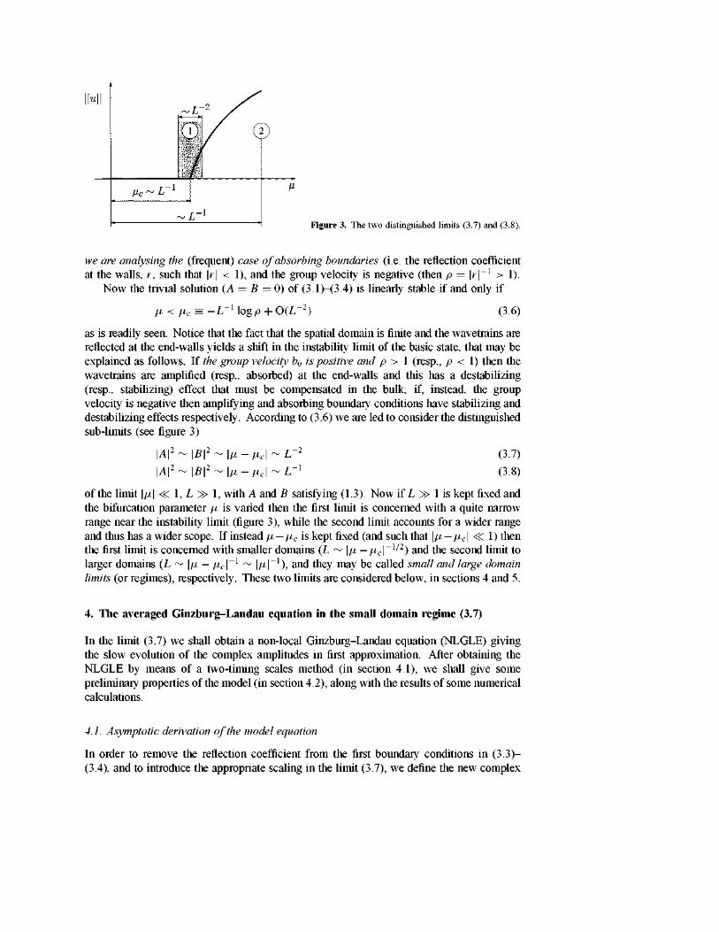
Figure 3. The two distinguished limits (3.7) and (3.!
we are analysing the (frequent) case of absorbing boundaries (i.e. the reflection coefficient at the walls, r, such that \r\ < 1), and the group velocity is negative (then p = |r|_1 > 1).
Now the trivial solution (A = B = 0) of (3.1)—(3.4) is linearly stable if and only if
p < pc -L-llogp + 0(L-2) (3.6)
as is readily seen. Notice that the fact that the spatial domain is finite and the wavetrains are reflected at the end-walls yields a shift in the instability limit of the basic state, that may be explained as follows. If the group velocity b0 is positive and p > 1 (resp., p < 1) then the wavetrains are amplified (resp., absorbed) at the end-walls and this has a destabilizing (resp., stabilizing) effect that must be compensated in the bulk; if, instead, the group velocity is negative then amplifying and absorbing boundary conditions have stabilizing and destabilizing effeets respectively. According to (3.6) we are led to consider the distinguished sub-limits (see figure 3)
\A\2
IAI2 \B\2>
\B\2' \p - pc
\p- pc
(3.7)
(3.8)
of the limit \p\ <¡C 1, L y¡> 1, with A and B satisfying (1.3). Now if L y¡> 1 is kept fixed and the bifurcation parameter p is varied then the first limit is concerned with a quite narrow range near the instability limit (figure 3), while the second limit accounts for a wider range and thus has a wider scope. If instead p-pcis kept fixed (and such that \p — pc\ -C 1) then the first limit is concerned with smaller domains (L ~ \p — pc\~
l/2) and the second limit to larger domains (L \P ~ Pc \p\ ), and they may be called small and large domain limits (or regimes), respectively. These two limits are considered below, in sections 4 and 5.
4. The averaged Ginzburg-Landau equation in the small domain regime (3.7)
In the limit (3.7) we shall obtain a non-local Ginzburg-Landau equation (NLGLE) giving the slow evolution of the complex amplitudes in first approximation. After obtaining the NLGLE by means of a two-timing scales method (in section 4.1), we shall give some preliminary properties of the model (in section 4.2), along with the results of some numerical calculations.
4.1. Asymptotic derivation ofthe model equation
In order to remove the reflection coefficient from the first boundary conditions in (3.3)-(3.4), and to introduce the appropriate scaling in the limit (3.7), we define the new complex
(4.3)
amplitudes, Y and Z, the re-scaled space and time variables, f and T, the new bifurcation parameter X and the small parameter e, as
A = epí+1/2Y exp[ia5tf + T + 1/2) + ie((a2 - a7)(logpf + a5(2 - a6)logp - a2a25)T]
(4.1)
B = epS+1/2Zexp[ia5(-% + T + 1/2) + ie((a2 - a7)(logpf
+a5(2-a6)logp-a2a25)T] (4.2)
f = ex T = et
¡j, = -elogp +s2[X + a25 + a5(2a2 - a7)logp - (1 + a 8 - a6)(logp)2]
e = \/L « 1 (4.4)
to write (3.1)-(3.4) as
YT = e(l + ia2)Yff + [1 + e « + ia'sWs + sYlx ~ (l + m)p1+2^\Y\2
- ( a 1 + i a 4 ) p 1 ^ | Z | 2 ] + 0 ( e 2 ) (4.5)
ZT = e(l + ia2)ZK - [1 + e « + ia's)]Zt¡ + eZ[X - (1 + i a s ) ^ 1 ^ | Z | 2
-(ü'1+iü'4)p1+2^|}'|2] + 0(e2) in - 1/2 < f < 1/2 (4.6)
7 = Z + 0(e2) at£ = ± l / 2 (4.7)
7? + Z? = ±e(p2 - 1)[1 - ttl + i(a3 - «4)]r |F I + 0(e2)
where
a'5 = (2a2 — aj) logp + 2a¡ a'6 = (2 — a,¡) logp — 2a2a¡. (4.8) Notice that the factors p^+l/2 and p^+l/2 have been introduced in (4.1), (4.2) for
the resulting problem to exhibit perfectly reflecting boundary conditions; this will allow us to apply a reflection principie and extend the spatial domain to — oo < f < oo (thus the characteristics of the leading hyperbolic problem are straight lines and the application of solvability conditions will be much facilitated). The other factors in (4.1), (4.2) are introduced to eliminate the phase shift in the reflecting boundary conditions, and to obtain equations on the new variables that are as simple as posible.
Now, to the leading order, Y and Z satisfy linear, first-order, wave equations (YT — Y¡= = ZT + Z¡: = 0 in - 1 / 2 < f < 1/2) with perfectly reflecting boundaries (Y = Z at f = ±1/2), and thus exhibit a linear, undamped, hyperbolic behaviour. Diffusion, dispersión and nonlinearity come into play in a second, still slower, time scale
x =eT (= e2í) (4.9)
and their effect is analysed by considering higher order terms
Y = Y0 + e y 1 + . . . z = Z0 + e Z 1 + - - - (4.10)
in (4.5)-(4.7). Then the following problems result:
Y0T - % = Z o r + Z0? = 0 (4.11)
YIT - Yit; = -Y0T + (1 + ia2)Y{)¡:¡: + (a'6 + ia'5)Y0í: + XY0
-Y0[(l + ia3)pl+2^\Y0\
2 + (al+ia4)pl-2^\Z0\
2] (4.12)
Zir + Zij = - Z 0 T + (1 + ia2)Z0ff - (a'6 + ia'5)Z0$ + XZ0
-Zo[(l + ia3)/t>1~2f|Zo|2-l-(oíi-|-ia4)/t>1+2f|l'ol2] in - 1/2 < £ < 1/2
(4.13)
at£ = ± l / 2 . (4.14) a4)]Y0\Y0\
2
Yo-
^
- Z 0 =
+ z l f
Y0¡: + Zo%
= T ( 1 - P :
= Y1
2 ) [ 1 -
- Z i = 0
- ax + i(a3
Notice that the second and fourth pairs of boundary conditions in (4.14) need not be imposed because they readily follow from (4.11)—(4.13) and the remaining boundary conditions. Equations (4.11)—(4.13) are invariant under space reflection f -> —f, Y0 o Z0, Y\ o Z i , and the boundary conditions (4.14) are appropriate to apply a reflection principie at % = ±1/2 to extend (4.11)-(4.14) to the whole line, -oo < % < oo, with a spatial periodicity condition (as it is convenient to solve (4.11)—(4.14) in the faster time scale). In order to do that we introduce the new dependent variables w0 and w\, defined in —oo < f < oo as
Wj^,T,r) = Zj(-l-^T,r) if - 3/2 < £ < - 1 / 2
Wj^,T,r) = Yj^,T,r) if - 1/2 < % < 1/2
Wj(% + 2, T, x) = Wj(%,T,r) if - oo < f < oo (4.16)
for j = O and 1, to rewrite (4.11)—(4.14) as
w o r - u>o¡¡ = O (4.17)
wlT - w^ = - W 0 T + (1 + ia2)w0^ + (cüg + ia'5)w0% + Xw0 - w0[(l + ia3)(p(^)\w0\2
+(«! + ia4)ít>(-f ) |w 0 ( - l - £, r , r)|2] (4.18)
where
(pg) = pl+2í¡ if - 1/2 < f < 1/2 T (4.19) ío(f + 1) = ÍÍ>(£ ) if - oo < f < oo
Notice that if O < p ^ 1 then <p exhibits jumps at f — 1/2 = integer and thus w^ is not smooth at these valúes of f. These jumps in w^ were to be expected and they are precisely such that the boundary conditions (4.14) are satisfied, as is readily seen when taking into account the reflection principie (4.15). Now, by integrating (4.17), (4.18) in the faster time scale we obtain
Wo = W(r¡, x) (4.20)
u>! = F{n, T) + tt/2)[-Wr + (1 + ia2)Wm + « + ia'5)Wn + kW] f (1-0/2
+(í+ia3)W\W\2 / (p(z)dz Jo
r (1-0/2 +(ai+ia4)W <p(-z)\W(r]-2z-l,x)\2dz (4.21)
Jo in terms of the characteristic variables
r] = T + i¡ and ? = T - f (4.22)
where the function F remains undetermined at this stage in the perturbation process. Finally, by eliminating secular terms, i.e. by requiring w\ to be bounded as T -> oo for each fixed valué of r], we get
Wx = (1 + ia2)Wm + (a<6 + ia'5)Wn + W - [(p2 - l)/(2logp)]W /.1/2
(l+ia3)\W\2 + (a,+ia4) / <p(z)\W(r¡ - 2z - 1, r) |2dz J—1/2
W(r] + 2,x) = W(r],x) if - oo < r¡ < oo (4.24)
(4.23)
where
0(z) = (21ogp)p 1 - 2 V(p 2 -D. (4.25)

To obtain (4.23) we have taken into account that, as T -> oo with r¡ fixed, f -> oo and (1-0/2
J( ^(z)dz = - ( p 2 - l)¿;/(41ogp) + 0(1) o f (1-0/2 M/2
/ <p(-z)\W(.r¡-2z-l,T)\2dz = -(U2) p^2z\W(r] - 2z-l, x)\2dz +0(1) J0 J —1/2
as readily seen when taking into account (4.16), (4.19) and (4.20). Finally, by using the new variables v and y, and the new bifurcation parameter j3,
defined as
v = W[(p2 - l)/(21ogp)]1/2exp[-iáí] + iá(áa2 - a'6)r] , 7 , (4.26)
y = T¡ + (a6 — 2&oi2)T ¡3 = X — S — 8a5
where
5 = -7r[integer part of(a'5/7t)]
equation (4.23) may be somewhat simplified to
vr = (1 + ia2)vyy + ia'¡vy
-v ,.1/2
0 - (l + ia3)|w|2 _ ( a i + ic<4) / <p(z)\v(y - 2z - 1, r) |2 dz -1/2
(4.27)
v(y + 2, r) = v(y, r) in — oo < y < oo (4.28)
with
a¡ = 27r[fractional part of ((a'5 + 7r)/27r))] - n. (4.29)
The averaged Ginzburg-Landau equation (4.27) depends on the bifurcation parameter j3 and on the real parameters
O < p < oo — oo < a¡ < oo for j = 1, . . . , 4 —7t^a'í<7t. (4.30)
Each solution of (4.27), (4.28) yields (a first approximation of) an evolution of the complex amplitudes A and B, that may be calculated in terms of the time scales T = et and r = e2í, when taking into account (4.1)-(4.4), (4.10), (4.15), (4.16), (4.20) and (4.26).
Notice that in the particular case of perfectly reflecting boundaries, p = 1, a removable singularity appears in (4.23) and (4.25). If the analysis above is repeated for that particular case (not considered independently for the sake of brevity) then it is readily seen that everythingstandsafterreplacing2(logp)/(p2-l)by 1; then the weight function <f> appearing in the averaged term becomes identically equal to 1.
The averaged term in (4.27) comes from the nonlinear cross-terms in (3.1), (3.2), that account for the effect of each wavetrain on the other (counterpropagating) one. It may be explained as follows. In the short time scale, T = et ~ 1, both counterpropagating wavetrains exhibit only linear propagation and reflection at the walls. The propagating velocity is large (of the order of e_1) in the slower time scale, x = e2t ~ 1. Thus, in the slower time scale each wavetrain 'sees' the other one travelling very fast in the opposite direction, and reflecting many times at the walls; only a weighted, averaged effect is felt in this time scale, the weight coming from the fact that the wavetrains are amplified (if p < 1) or reduced (if p > 1) as they travel, in order to counterbalance the instantaneous reduction (if p < 1) or amplification (if p > 1) at the walls.
A complete parametric description of the attractors (as x ->- oo) of (4.27), (4.28) is expected to be extremely complex due to both the presence of diffusion, dispersión,

nonlinearity and mean-field eífects, and the large number of parameters involved. Instead, some remarkable features will be outlined now. For a more complete analysis of (4.27), (4.28), see [42].
4.2. Some properties ofthe averaged Ginzburg-Landau model
A rigorous derivation of the averaged Ginzburg-Landau problem (4.27), (4.28) for the particular case of perfectly reflecting boundaries, p = 1, was given in [39], along with several global properties ofthe solutions. The ideas in [39] may be extended to the general case p T¿ 1, to prove, in particular, that if initial data is prescribed, then (4.27), (4.28) define a unique solution, that is uniformly bounded fora l l r > 0 if «i > — 1. If «i < - 1 (resp., «i = — 1) then (4.27), (4.28) possess solutions that blow up in finite time (resp., as x -> oo), as is readily seen when considering spatially uniform solutions, that are such that V = | v | satisfy the following ODE:
áV/áx = [fi -(l + ai)V2]V.
Then, if a\ < - 1 (resp., a\ = -1 ) local bifurcation at the onset ofthe oscillatory instability is sub-critical (resp., critical) and the analysis ofthe large-time dynamics ofthe underlying physical system requires that we consider the fully nonlinear model (resp., requires that we consider higher order nonlinear terms in the amplitude equations). In what follows, we shall consider only the super-critical case, ct\ > —1.
The simplest solutions of (4.27), (4.28) are such that \v\ is constató, and are given by
v = R0 exp(iq0x + ipoiry) (4.31)
where the real parameters R0 > 0 and q0 are given by
*0 = lfi~ (POX)2 -< (p 0 JT) ] / ( l + « l ) q0 = -a2(po7tf - (a3 + a^R2,
and po is an arbitrary integer. Notice that (i) there are infinitely many branches of these solutions that bifúrcate (through pitchfork bifurcations) from the basic steady state, v = 0; (ii) these solutions are independent of the reflection coefficient p; and (iii) the associated solutions of the amplitude equations are fairly simple, such that \A\ = eR0p^+l/2 and |B| = eR0p-^+ll2 to a first approximation (see (4.1)-(4.4), (4.10), (4.15), (4.16), (4.20) and (4.26)). The (straightforward but tedious) linear stability analysis of these solutions provides some insight into the large-time dynamics of (4.27), (4.28) (see [42]). According to the consistency conditions (1.3), only a large but finite number of the infinitely many branches mentioned above correspond to approximate solutions of the underlying physical problem. These solutions are associated with the different possible valúes of the phase shifts of the complex amplitudes (of the counterpropagating wavetrains) between the end-walls, and (somehow) account for the discrete distribution of wavenumbers due to the fact that the spatial domain is large but finite.
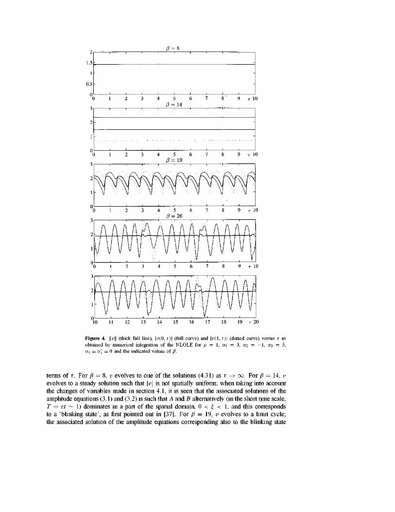
Let us first consider the particular case of perfectly reflecting boundaries, p = 1. If l+a2a3 < 0 and /3 > 0 is not too small then all solutions (4.31) are unstable (they exhibit the modulational instability, as the simplest solutions ofthe standard Ginzburg-Landau equation do). Then the dynamics of (4.27), (4.28) is expected to be fairly complex, as shown in figure 4, where representative results are given that were obtained by numencal integration of (4.27), (4.28) in the particular case p = 1, a\ = 3, a2 = — 1, a3 = 5, a4 = a¡ = 0, for several valúes of the bifurcation parameter j3. In order to appreciate the spatial stracture of \v\ to some extent, we have plotted ||u|| = [J_j \v(y, r) |2dy/2] , |u(0, T) | and \v(l, r)\ in
0 = 8
) 1 2 3 4 5 >3 = 14
6 7 8 9 r 1
-
-
-
-
8 9 r 10
9 r 10
9 r 10
10 11 12 13 14 15 16 17 18 19 T 20
Figure 4. ||i>|| (thick íüll line), |i>(0, r ) | (full curve) and |u(l, r ) | (dotted curve) versus r as obtained by numerical integration of the NLGLE for p = 1, a\ = 3, a?2 = —1, «3 = 5, «4 = OÍ'Í = 0 and the indicated valúes of /?.
terms of r. For /i = 8, v evolves to one of the solutions (4.31) as r -> oo. For f¡ = 14, v evolves to a steady solution such that \v\ is not spatially uniform; when taking into account the changes of variables made in section 4.1, it is seen that the associated solutions of the amplitude equations (3.1) and (3.2) is such that A and B alternatively (in the short time scale, T = et ~ 1) dominates in a part of the spatial domain, 0 < f < 1, and this corresponds to a 'blinking state', as first pointed out in [37]. For j3 = 19, v evolves to a limit cycle; the associated solution of the amplitude equations corresponding also to the blinking state

whose structure now periodically evolves also in the slower time scale, x = e2t ~ 1. For ¡i = 26 the solution exhibits an intermittent behaviour as x -> oo. After an interval of time when the profile behaves as a travelling wavetrain (the associated solutions of the amplitude equations corresponding to slowly modulated blinking states, as above), sudden excursions to more complex behaviour take place (at x ~ 3, 6.5, 9.5,...) in an aperiodic way. Such intermittent behaviour has also been obtained for the standard Ginzburg-Landau equation [56]; as in [56], for very large valúes of /3, the solution of (4.27), (4.28) is expected to exhibit spatio-temporal intermittency, that will be considered in [42]. If 1 + a2a3 > 0, then the steady states (4.31) exhibit again instabilities for appropriate valúes of the remaining parameters, that are not considered here for the sake of brevity; if, in addition, j3 is large, then the solutions of (4.27), (4.28) are expected to exhibit a simple behaviour as suggested by the solutions in the second regime that will be considered in section 5.
If p T¿ 1, then the analysis of the linear stability of the solutions of (4.31) is quite tedious. Here we only point out a remarkable feature concerning the limits p -> 0 and p -> oo, that may be easily explained. If either p y>> 1 or p <C 1, then the weight function <f> appearing in the averaged term of (4.27) is cióse to a Dirac delta function, and (4.27) becomes the following standard Ginzburg-Landau equation:
vr = (1 + ia2)vyy + \a'¡vy + v[f) - (1 + «i + i(a3 + a4))M2]-
For this approximation to be valid, the bifurcation parameter j3 cannot be too large if p remains fixed (for, if /i is large then \vy\ is also large and the local approximation of the non-local averaged term fails). Then if 1 + «2(«3 + «4)/(l + «i) < O and j3 > O is neither too large ñor too small, then the solutions (4.31) exhibit the modulational instability; consequently, a complex dynamic behaviour is to be expected for intermediate valúes of j3. Numerical integrations of (4.27), (4.28) show that this is in fact the case, as shown in figure 5, for the particular case p = 100, a\ = 3, a2 = — 1, a3 = 0, a4 = 6 and a'¡ = 0. As in figure 4, ||u||, |u(0, x)\ and |u(l, x)\ are plotted in terms of x for several valúes of the bifurcation parameter j3.
5. The real nonlinear wave system in the large domain regime (3.8)
In the limit (3.8) we re-scale the amplitudes, the space and time variables and the bifurcation parameter as
A = e1,2Y B=e1,2Z x = l¡/e t = T/e p = ek (5.1)
in terms of the small parameter
s = l/L « 1 (5.2)
to re-write (3.1)—(3.4) as
YT = e(l + i a 2 ) % + Yf + Y[X - (1 + ia 3 ) |F | 2 - (a, + ia4)\Z\2] +HOT (5.3)
ZT = e(l + ia2)ZK -Zf + Z[X - (1 + ia3)\Z\2 - (a, + ia4)\Y\2] + HOT
in - 1/2 < f < 1/2 (5.4)
Z = péa5Y + eHOT at f = - 1 / 2 Y = peia5Z + eHOT at f = 1/2 (5.5)
Zi;+pQ10í5Yi: = pQ10í5(l-p2)[l-a1+i(a3-a4)]Y\Y\2+¥íOT at f = - 1 / 2 (5.6)
Y¡: + pem'Z>: = PQm'(p2- l ) [ l -o ! i + Í ( Ü ' 3 - Ü ' 4 ) ] Z | Z | 2 + H O T at f = 1/2 (5.7)
where
HOT = 0[e(X + \Y\2 - |Z|2)(|7,| + \Z*\) + e(X + \Y\2 + \Z\2f(\Y\ + |Z|)].

/3 = 20
2~
9 T 10
ftti'cl 11 W J w
j(|nW,|lWri(,|
•V |«
AWitt'l 1
I " O T
• l ' i
I r ' JiPwmi
l Ir ' ultaflllp1
ri] M\n; í N*
i/ V ' V\ ' | ' l l | | ' i ;V l ti
w Mf ***vVi
1
8 9 r 10
c 8
6
2
1 2 3 4 5 6 ,3 = 200
? 8 9 r 1
' i i 1 i
-
-
0 1 2 3 4 5 6 7 8 9 r l 0
Figure 5. As in figure 3 but for p = 100, u\ = 3, ai = — 1, a¡ = 0, a\ = 6, a'¿ = 0 and the indicated valúes of /?.
The solutions of (5.3)-(5.7) such that
| e % | « 1 and \eZff\ « 1 (5.8)
for all T > 0, T ~ 1, depend only on the spatial scale f ~ 1 and may be obtained by seeking for an expansión of the form
Y = Y0G,T) + eY1G,T) + --- Z = Z0^,T) +eZ^,T) + • •• (5.9)
where the leading order terms are readily found to be given by the hyperbolic system
Y0T = Y^ + Y0(k - (1 +ia3) |F0 |2 - («i + ia4)\Z0\2) (5.10)
ZOT = -Zol: + Zo(k-(l + ia3)\Zo\2-(a1+ia4)\Yo\2) in - 1/2 < £ < 1/2
(5.11)
Z0 = peiOÍ5Y0 a t f = - l / 2 70 = peia5Z0 a t f = 1/2. (5.12)
That system will be considered in section 5.2. Here we only point out that althougth the boundary conditions (5.6), (5.7) cannot be imposed on Y0 and Z0, they are precisely such that every solution of (5.10), (5.11) satisfies them for all T > 0 provided that these conditions hold at T = 0. Then no boundary layer is necessary near í¡ = ±1/2 to impose (5.6), (5.7). This fact is essential for the consistency of our weakly nonlinear description. If the boundary conditions (5.6), (5.7) were not satisfied by the solutions of (5.10), (5.11), then two boundary layers would be necessary near f = ±1/2; the characteristic size of those layers should be such that \Y^\ ~ \Y%\ and \Z^\ ~ |Zj|, i.e. |f ± 1/2| ~ e, or \x ± L/2\ ~ 1; then the boundary layers would be precisely those considered in section 2.2 (where (5.3), (5.4) do not apply, see section 2.2) that allowed us to obtain the boundary conditions (5.6), (5.7).
Notice that conditions (5.8) mean that the smaller spatial scales are large as compared to s112 = L~112 in the f-variable (or to Le112 = L112 in the original x-variable). If condition (5.8) does not hold, then Y and Z depend on smaller spatial scales (than those of the size of the domain, f ~ 1 or x ~ L) and the approximation (5.9) breaks down That case will be considered elsewhere [44]. Here, we only derive sufficient conditions for (5.8) to hold in the time scale T ~ 1 provided that it holds at T = 0. To do that, in section 5.1 we shall analyse the linear evolution of an small perturbation (added to a solution of the type (5.9)) not satisfying (5.8). If all such perturbations are damped out exponentially as T -> oo, then we conclude that the approximation (5.9) makes sense for appropriate initial conditions.
The size of the small scales mentioned above is of the order of Ll/2 in the original x-variable; then these scales are in between that of the basic smallest scale, x ~ 1, and the size of the domain, x ~ L, and will be called intermedíate scales in the remainder of this paper.
5.1. Linear evolution ofincipient intermedíate scales
In order to analyse the linear evolution of small perturbations containing intermediate scales (i.e. not satisfying (5.8)) around a solution without those scales (i.e. satisfying (5.8)), we first anticipate that those scales are such that s\Y^\ ~ \Y\ ~ 1, e\Z^\ ~ \Z\ ~ 1, \Y%\ ~ \YT\ and |Zj| ~ \ZT\. Then we introduce the new short space and time variables
rj = e-1,2l; a=e-1,2T (5.13)
and consider a solution of (5.3)-(5.7) of the form
r(£, T; r¡, a) = [r0(£, T) + • • -][1 + yiH, T;r¡,a) + .. •]
Z(M, T; r,, a) = [Z0(f, T) + • • -][1 + z(f, T; r¡, a) + • • •]
where Y0 and Z0 is a given solution of (5.10)-(5.12) and
e « | 3 ' | « l e « | z | « l . (5.15)
By inserting (5.14) into (5.3)-(5.7) and taking into account (5.13) and (5.15), we get the following linear problem giving the evolution of y and z:
ya~yr, = sl/2[-yT + y^ + (l + ioc2)ym - (1 + ia3)\Y0\2(y + y)
- ( a 1 ± i a 4 ) | Z 0 | 2 ( z ± z ) ± H O T ] (5.16)
Za + Zr, =£1/2[-ZT ~ Z% + (1 + \a2)zm — (1 + ÍQf3)|Z0|2(z + z)
-(a,+ia4)\Y0\2(y + y)+ROT] (5.17)
in —1/2 < f < 1/2, —£~1/2/2 < r¡ < e1/2/2, with boundary conditions
z = y + e HOT
y, + z, = - e 1 / 2 [ ^ + zf ± p-2Hfi2 - 1)(1 - «i + i(a3 - «4))|i'o|2(3' + y) + HOT]
at % = ±1/2, r¡ = ±e-1'2/2, where HOT = 0(e + \y\2 + \z\2). In fact, only the first pair of boundary conditions (5.18) will be imposed below; the second pair is readily seen to hold, up to the order e1/2, as a consequence of the first pair and (5.16), (5.17) (notice that ym = Zr¡r¡ to the leading order at the boundanes, see (5.19) and (5.20) below). The solution of the complex linear problem (5.16)—(5.18) may be written as
/>O0
y= / [%+(f,r)e l t ("+ff ) + %(f,r)e- l t ( ' '+ff )]dfe + e
1 / 2 3 ' i ( f , r ; í ] , a ) + . . . (5.19) JO
/»00
/ [z+(£, D e * ^ + zt-(£, T)e-lk(i-a)] dfe + e1/2Zl (£, T; r¡, a) + • • • (5.20)
Jo
/o
z
where y¡ and z\ satisfy /»00
yia - ?i„ = / V-ytr + y» -k2(l + ia2)yt ~(l + ™3)\Y0\2{y+ + %)\ék
JO />O0
+ / 1-ytT + % " * 2 d + i«2)% - (1 + ia3)\Y0\2(y¿ + y+)]e-I*("+ff) dfe
Jo /»00
+ / NRTdfe (5.21) Jo
/>O0
zia + 2 1 , = / [-zt+
r - zt - fe2(l + ia2)zt+ - (1 + ia3)|Z0|2(zt+ + z ^ e * ^ dfe
Jo />oo
+ / [-z¿"r " z« " * 2 d + >«2)zt~ - (1 + i«3)|Zo|2(z^ + zt+)]e-I*("-ff) dfe
Jo
NRTdfe. (5.22) Jo lo
Here overbars and NRT stand for the complex conjúgate and non-resonant terms (i.e. terms not proporcional to exp[±ik(r¡ - a)] and to exp[±ik(r¡ + a)] in (5.21) and (5.22), respectively). Notice that y^ and zk account for the linear evolution of the intermedíate scale with a wavenumber equal to fe. By eliminating secular terms in (5.21) and (5.22) (i.e. by requiring y\ and z\ to be bounded in the time scale a ~ 1) we get, for all fe > 0,
y£T = y% - k2(l + ia2)yt - a + ^Wo\2{y^ + ykT) (5.23)
4r = " 4 " * 2 d + ia2)zt - (1 + i«3)|Z0| V + z*T) in - 1/2 < £ < 1/2
(5.24)
while the first boundary conditions (5.18) yield
% + =z t -e T h * %=z , + e ± I U t a t f = ± l / 2 (5.25) where vk = 2n fract(feVL/2;r), with fract(x) = fractional part of x.
In order to obtain equations and boundary conditions with real coefficients (and to eliminate the phase vk) we may use the new variables
4 = (%+ + %)e'^+r) vt = i(yk- - ytWv^+T)
(5.26) k "T- zk ;c ^ = i w t - ¿ t
w " t v ? T Í ; (z+ + z r ) e "*«+ r ) ur = i(z+ - z r ) e "*«+ r )

to write (5.23)-(5.25) as
4T - ut% = ~(k2 + 2\Y0\2)u+ + a2k
2v+ (5.27) vkT ~ u*+? = - ( « 2 ^ + 2a3\Y0\
2)u+ - k2v+ (5.28)
HT + ul% = ~^2 + 2\zo\2)ut + a2k2v^ (5.29)
vkT + ^ = -(«2¿2 + 2a3\Z0\2)uk - k2vk - 1/2 < % < 1/2 (5.30)
4 = H 4 = vk atf = ±l/2. (5.31)
Now, by collecting the results of the formal analysis above we may state the following properties concerning the stability of the solutions of (5.10)-(5.12) under small perturbations containing the intermediate scales. Take a solution of (5.10)-(5.12), Y0 = Y0{¿¡, T) and Z0 = Z0(£, T).
Property 1. If, for each k > 0, every solution o/(5.27)—(5.31) is such that
uk -> 0 and vk -> 0 exponentially as T -> oo f5.32j
;7ze« a«y small perturbation of {Yo, Zo) containing the intermediate scales is damped out exponentially as T -> oo. /« / t e case we conclude that {Yo, Zo) /'s a gooa" approximation of a solution q/"(5.3)-(5.7) /'« //ze ft'/we 5ca/e r ~ 1.
Property 2. /£ _/br so/we k > 0 ;7zere z's a solution of (5.27)—(5.31) //za/ diverges exponentially as T -> oo, z'.e. swc/z //za/ í/zere z's a sequence {(f„, T„)} satisfying —1/2 ^ f„ ^ 1/2, r„ ^ w/or a// « a«íi
l«í(fn, r„)| + |w¡T(t„, r„)| + |i^(f„, T„)| + |u^(f„, T„)\ -> oo exponentially as n -> oo.
(5.35)
77ze« ;7zere are small perturbations of{Yo, Zo), containing the intermediate scales, that do not remain smallfor all T > 0. In this case, we conclude that {Yo, Zo) cannot be considered a good approximation of a solution o/"(5.3)-(5.7) in the time scale T ~ 1.
Notice that although uk and vf are complex, their real and imaginary parts also satisfy (5.27)-(5.31) (because the coefficients in the equations and boundary conditions are real). Then we may consider uf and vf as real functions when analysing whether they satisfy one of the conditions (5.32) or (5.33).
The linear problem (5.27)-(5.31) is considered in appendix B, where sufficient conditions are obtained for properties 1 and 2 to apply (see theorem B.5 at the end of the appendix). Several remarks concerning the results in this section and those in appendix B are in order:
(a) The problem (5.27)-(5.31), giving the linear evolution of the intermediate scales, depends explicitly only on a2 and a3 (of course there is an implicit dependence o n p , I and «i through the functions \Y0\ and |Z0|).
( « ) (b)
( ' • )
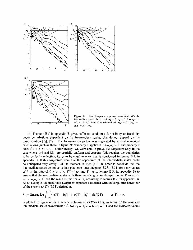
Figure 6. First Lyapunov exponent associated with the intermedíate scales. For l = 6, ai = 3, ai = 1, 1 + «2«3 = - 2 , - 1 , 0, 1, 2, 5 and 10 as indicated and (a) p = .01, (b) p = 1 and (c) p = 100.
(b) Theorem B.5 in appendix B gives sufficient conditions, for stability or instability under perturbations dependent on the intermedíate scales, that do not depend on the basic solution \Y0\, \Z0\. The following conjecture was suggested by several numencal calculations (such as those in figure 7): 'Property 1 applies if 1 + a2a3 > 0, and property 2 does if 1 + a2a3 < 0'. Unfortunately, we were able to prove the conjecture only in the case where \Y0\ and |Z0| are spatially uniform and constant (this requires the boundaries to be perfectly reflecting, i.e. p to be equal to one), that is considered in lemma B.l, in appendix B. If this conjecture were trae the appearance of the intermediate scales could be anticipated very easily. At the moment, if a2a3 > 1, in order to conclude that the intermediate scales do not come into play, one must intégrate (5.27)-(5.31) for many valúes of k in the interval 0 < k < (p,F*)112 {p, and F* as in lemma B.3, in appendix B) to ensure that the intermediate scales with these wavelengths are damped out as T ->- oo (if - 1 < a2a3 < 1 then the result is trae for all k, according to lemma B.2, in appendix B). As an example, the máximum Lyapunov exponent associated with the large time behaviour of the system (5.27)-(5.31), defined as
,.1/2 XL=limsuplog / (\u+\2 + \v+\2 + \u-k\
2+\v^\2)ó¿;/(2T) as T -+ oo J —1/2
is plotted in figure 6 for a generic solution of (5.27)-(5.31), in terms of the re-scaled intermediate scales wavenumber k2, for a\ = 3, X = 6, a2 = - 1 and the indicated valúes
IVII II 7
IVII 117 \x 11)11^
IVII 117
IVII 117 \i , \\¿j
IIVII 117 l l r II) 11^
IVII 117 r > I ^
1 + a2«3 = 1
O 5 10 15 20 25 30 35 40 45 r p 5 0
1 + a.io.% — ~ 1
O 5 10 15 20 25 30 35 40 45 rr>50 rpy
1 + a 2 a 3 — — 2
O 5 10 15 20 25 30 35 40 45 rpSO Ts
1 + 020:3 = —5
O 5 10 15 20 25 30 35 40 45 r p 5 0 T1
0.5
Solution of Hyperbolic Eqs.
/ 10 15 20 25 30 35 40 45 rr>50 rpSi
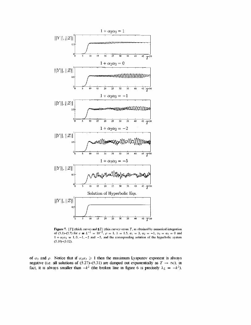
Figure 7. \\Y\\ (thick curve) and ||Z|| (thin curve) versus T, as obtained by numerical integration of (5.3)-(5.7) for e = L~l = 10~2, p = 1, k = 1.5, ai = 3, a?2 = —1, «4 = «5 = 0 and 1 + a2«3 = 1 , 0 , - 1 , - 2 and —5, and the corresponding solution of the hyperbolic system (5.10)-(5.12).
of «3 and p . Notice that if a2a3 > 1 then the máximum Lyapunov exponent is always negative (i.e. all solutions of (5.27)-(5.31) are damped out exponentially as T -> oo); in fact, it is always smaller than —k2 (the broken line in figure 6 is precisely XL = —k2).
0 -
0.5 -i
1 i
1.5 i
2
T 2.5
3-i
3.5 r
4-;
4.5 h
5 -
-0.5 0 0.5 -0.5 0 0.5
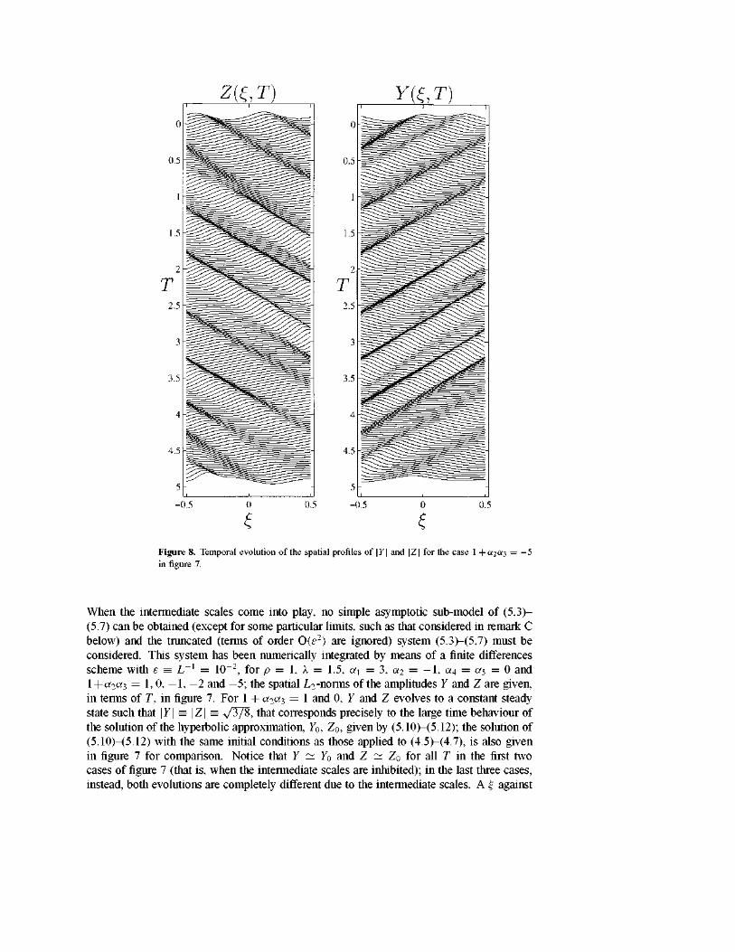
Figure 8. Temporal evolution of the spatial profiles of |F| and \Z\ for the case 1+012013 = —5 in figure 7.
When the intermedíate scales come into play, no simple asymptotic sub-model of (5.3)-(5.7) can be obtained (except for some particular limits, such as that considered in remark C below) and the truncated (terms of order 0(e2) are ignored) system (5.3)-(5.7) must be considered. This system has been numerically integrated by means of a finite differences scheme with e = L_ 1 = 10~2, for p = 1, X = 1.5, a\ = 3, a2 = —1, a4 = a5 = 0 and l + a2a3 = 1, 0, —1, - 2 and - 5 ; the spatial L2-norms of the amplitudes Y and Z are given, in terms of T, in figure 7. For 1 + a2a3 = 1 and 0, Y and Z evolves to a constant steady state such that \Y\ = \Z\ = V3/8, that corresponds precisely to the large time behaviour of the solution of the hyperbolic approximation, Y0, Z0, given by (5.10)-(5.12); the solution of (5.10)-(5.12) with the same initial conditions as those applied to (4.5)-(4.7), is also given in figure 7 for comparison. Notice that Y ~ Y0 and Z ~ Z0 for all T in the first two cases of figure 7 (that is, when the intermedíate scales are inhibited); in the last three cases, instead, both evolutions are completely different due to the intermedíate scales. A f against
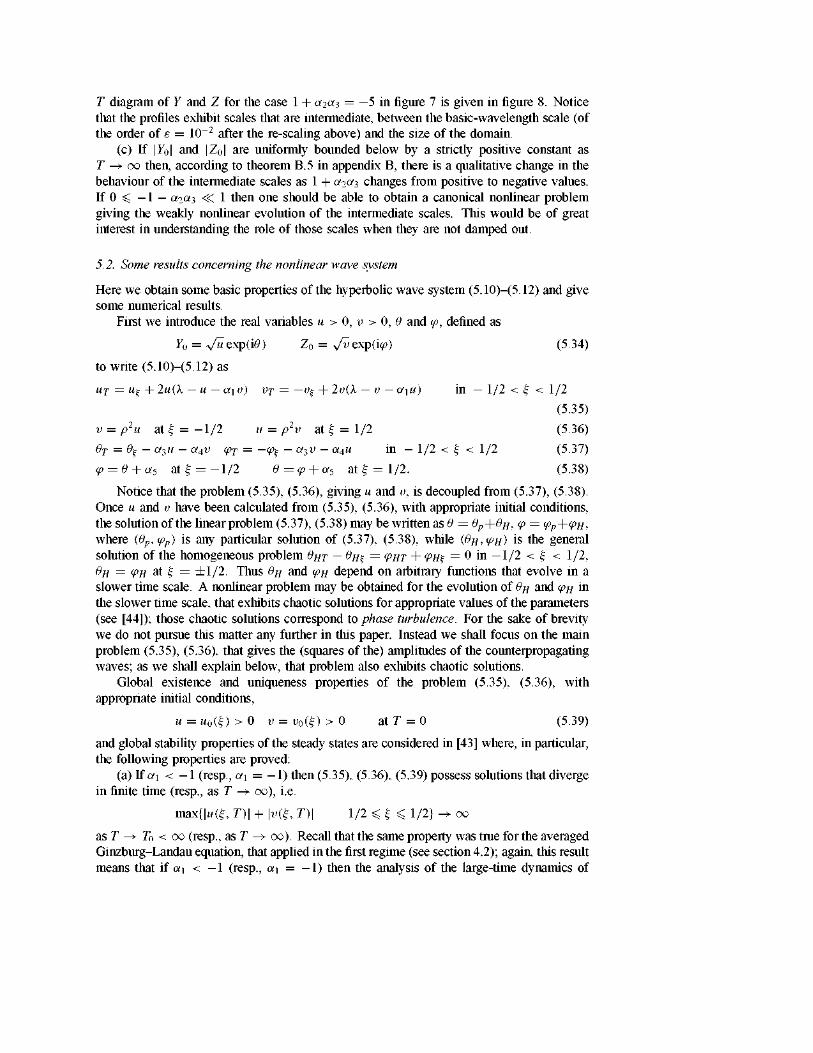
T diagram of Y and Z for the case 1 + a2a3 = -5 in figure 7 is given in figure 8. Notice that the profiles exhibit scales that are intermedíate, between the basic-wavelength scale (of the order of e = 10~2 after the re-scaling above) and the size of the domain.
(c) If | Y01 and |Z0| are uniformly bounded below by a strictly positive constató as T -> oo then, according to theorem B.5 in appendix B, there is a qualitative change in the behaviour of the intermediate scales as 1 + a2a3 changes from positive to negative valúes. If O < - 1 - a2a3 <C 1 then one should be able to obtain a canonical nonlinear problem giving the weakly nonlinear evolution of the intermediate scales. This would be of great interest in understanding the role of those scales when they are not damped out.
5.2. Some results concerning the nonlinear wave system
Here we obtain some basic properties of the hyperbolic wave system (5.10)-(5.12) and give some numerical results.
First we introduce the real variables u > O, v > O, 0 and <p, defined as
Y0 = */u exp(i0) Z0 = v/uexp(i^) (5.34)
to write (5.10)-(5.12) as
UT = ui: + 2w(A. — u — a\v) vj = —v^ + 2i>(A. — v — a\u) in — 1/2 < f < 1/2
(5.35)
v = p2u at f = - 1 / 2 u = p2v at f = 1/2 (5.36)
0T = 0% — ce3u — a4v <px = —<p^ — a3v — a4u in — 1/2 < f < 1/2 (5.37)
(p = e + a5 a t f = - l / 2 e=cp + a5 at f = 1/2. (5.38)
Notice that the problem (5.35), (5.36), giving u and v, is decoupled from (5.37), (5.38). Once u and v have been calculated from (5.35), (5.36), with appropriate initial conditions, the solutionof the linear problem (5.37), (5.38) may be written as 6 = 9P+9H, <p = <PP+<PH,
where {9p,(pp) is any particular solution of (5.37), (5.38), while (0H,'PH) is the general solution of the homogeneous problem 0HT - OH% = <PHT + <PHÍ¡ = O in - 1 / 2 < f < 1/2, OH = <PH at f = ±1/2. Thus OH and <pn depend on arbitrary functions that evolve in a slower time scale. A nonlinear problem may be obtained for the evolution of 9H and <pH in the slower time scale, that exhibits chaotic solutions for appropriate valúes of the parameters (see [44]); those chaotic solutions correspond to phase turbulence. For the sake of brevity we do not pursue this matter any further in this paper. Instead we shall focus on the main problem (5.35), (5.36), that gives the (squares of the) amplitudes of the counterpropagating waves; as we shall explain below, that problem also exhibits chaotic solutions.
Global existence and uniqueness properties of the problem (5.35), (5.36), with appropriate initial conditions,
M = M o ( f ) > 0 u = i;o(f)>0 a t r = 0 (5.39)
and global stability properties of the steady states are considered in [43] where, in particular, the following properties are proved:
(a) If a\ < - 1 (resp., a\ = -1 ) then (5.35), (5.36), (5.39) possess solutions that diverge in finite time (resp., as T ->- oo), i.e.
max{|íí(f, T)\ + \v(%, T)\ 1/2 ^ f ^ 1/2} -^ oo
as T -+ T0 < oo (resp., as T -+ oo). Recall that the same property was true for the averaged Ginzburg-Landau equation, that applied in the first regime (see section 4.2); again, this result means that if «i < - 1 (resp., a\ = - 1 ) then the analysis of the large-time dynamics of

1.6
1.4
1.2
U \ \ l \\V\\ 1
0.8
0.6
0.4
0.2
Al Al A3 A
Figure 9. Bifurcation diagram of the nonlinear wave system (5.35), (5.36) for p = 0.1 and u\ = 3.
the underlying physical system requires that we consider the fully-nonlinear model (resp., requires that we consider higher order terms in the amplitude equations).
(b) If a\ > - 1 then every solution of (5.35), (5.36), (5.39) is uniformly bounded in - 1 / 2 < f < 1/2, 0 < T < oo. If, in addition X < - logp then \u\ + \v\ -> 0, uniformly in - 1 / 2 < f < 1/2, as T ^ oo.
(c) If — 1 < «i < 1 and X > - l o g p then (5.35), (5.36) has a unique steady state, (us, vs), such that us > O and vs > O in - 1 / 2 < f < 1/2, and every solution of (5.35), (5.36), (5.39) is such that u -> us and v -> vs, uniformly in —1/2 < f < 1/2, as T -+ oo.
Global stability properties are obtained in [43] by means of comparison methods that do not apply if a\ > 1 and X > - log p. This case is considered in [44], where continuation methods, standard dynamical systems techniques and numerical integration of (5.35), (5.36) are systematically used. As an example of the results obtained in [44], the attractors (as T ->- oo) of (5.35), (5.36) are plotted in figures 9 and 10 in terms of the bifurcation parameter X for the particular case a\ = 3 and p2 = 0.1. As shown in figure 9, at X = A.1 = — logp ~ 1.15 there is a supercritical bifurcation from the basic steady state, u = v = 0, to a new branch of symmetric steady states (i.e. invariant under the symmetry u -+ v, v -+ u, x ->- —x). As an example, the bifurcated steady state for X = 2 is plotted in figure 10(a); when taking into account the fact that */u and */v are essentially the modulating amplitudes of two counterpropagating wavetrains (see (2.13), (5.1), (5.9) and (5.34)), these bifurcated steady states are seen to correspond to symmetric chevrons in the spacetime diagram of the underlying physical problem. At X = X2 — 2.70 there is a secondary supercriticalpitchfork bifurcation to non-symmetric steady states (i.e. a symmetry breaking); as an example, one of the two non-symmetric steady states at X = 3 is plotted in figure 10(6), and corresponds to a non-symmetric chevron. At X = X3 ~ 3.35 there are two super-critical Hopf bifurcations (one from each branch of non-symmetric steady states) to non-symmetric limit cycles; that for X = 3.5 is plotted in figure 10(c). Its period is T0 ~ 3.09, and corresponds to a beating state (essentially only one of the two counterpropagating wavetrains is seen in most part of the domain, and the size of this part

0.6
¡i, V ' 0,4
0.2
0 -0.5 -0.4 -0.3 -0.2 -0.1 0 0.1 0.2 0.3 0.4 ¿. 0.5
(*) _ _
-0.5 -0.4 -0.3 -0.2 -0.1 0 0.1 0.2 0.3 0.4 t 0.5
Figure 10. Attractors as T —>• oo of the nonlinear wave system for the case in figure 9 and (a) 1 = 2, (b) 1 = 3 and (c) A. = 3.5 («: solid curve and v: dotted curve).
varíes periodically in time; the other wave is seen only in a quite narrow región). The remaining part of the bifurcation diagram is not precisely descnbed here for the sake of brevity. Let us just say that for larger valúes of X there is a period-doubling sequence that leads to a non-symmetric a chaotic attractor that, as X mercases, becomes symmetric; as X is further increased the attractor becomes periodic through an intermittency-like process. This way of gaining symmetry through chaos is known as crisis. For higher valúes of X, symmetry is lost again through a transcritical bifurcation and a second crisis takes place as X is further increased. See [44] for details. For other valúes of the parameters p > 0 and «i > 1, bifurcation diagrams in terms of X are qualitatively similar to that descnbed above.
6. Concluding remarks
The amplitude equations that apply at the onset of the oscillatory instability in large domains, and the appropriate boundary conditions when the domain is finite, have been obtained for ID reaction-diffusion systems in section 2, and for more general problems in appendix A. In the generic case when the group velocity is of order unity, the amplitude equations contain terms that are not of the same order. This fact has allowed us to obtain two asymptotic submodels in the distinguished limits (3.7) and (3.8). In the first distinguished limit we have reduced the amplitude equations to an averaged Ginzburg-Landau model, that accounts for diffusion, dispersión, nonlinearity and interaction of each wavetrain with a weighted average of the counterpropagating one. That model was obtained in section 4.1, and some of its properties were briefly considered in section 4.2; a more complete analysis of the model will be given elsewhere [42]. In the second distinguished regime, the real amplitudes and phases associated with the complex amplitudes become decoupled in the first approximation provided that some intermedíate scales (whose wavelength is large compared with the basic wavelength of the counterpropagating wavetrains, but small compared with the size of the spatial domain) are inhibited; a linear model giving the incipient evolution of the intermediate scales was obtained in section 5.1 and analysed in appendix B, where sufficient conditions were derived for the intermediate scales to be exponentially damped out for large time. When the intermediate scales are inhibited, the evolution of the real amplitudes of the counterpropagating wavetrains is given by a system of two nonlinear wave equations that account for wave propagation and nonlinear interaction, with boundary conditions accounting for linear reílection at the boundaries; that system is thoroughly

(c)
u,v 2
i
T = = 0
_ _ _ _ _ _ _ _ • - " " :
u,v
u,v
-0.5 -0.4 -0.3 -0.2 -0.1 0 0.1 0.2 0.3 0.4 ¿- 0.5 Figure 10. (Continued.)
analysed in [43,44] and briefly discused in section 5.2. We believe that our results provide a fairly complete picture of the weakly nonlinear
behaviour of physical systems near the onset of the oscillatory instability. Qualitative and quantitative companson with experimental results in the literature [41,44] are fairly good.

Notice that our analysis predicts two main sources of complexity: (a) The modulational instability in the first distinguished regime, and the appearance of
the intermedíate scales in the second distinguished limit, that come into play whenever
1 + a2a3 < 0.
(b) The presence of the walls. Inthe first distinguished regime, the averaged Ginzburg-Landau model exhibits complex behaviour if 1 + a2a3 > 0 but the remaining parameters are appropriate. In the second distinguished regime, the hyperbolic system exhibits chaotic behaviour if a\ > 1 and X is appropriate.
Finally, let us just mention two obvious extensions of our results, that will be considered elsewhere.
• If the governing equations are still invariant under reflection (and translation) but the boundary conditions at x = ±L/2 are not, then the amplitude equations (3.1), (3.2) still apply, but the reflection coefficient, pe1"5, is not the same in both boundary conditions (3.3) and (3.4). This extensión is of interest in some experiments; for example, in the Taylor-Couette system, the upper end of the liquid in between of the counter-rotating cylinders is sometimes left open.
• As mentioned in section 1, if the spatial domain has no boundaries (e.g. if it is an annulus) then the boundary conditions (1.4)—(1.6) must be replaced by (1.4'). Then the distinguished limits (3.7), (3.8) must be still considered, with /xc = 0. In the first distinguished limit, a system of two Ginzburg-Landau equations is obtained, with non-local averaged coupling terms. In the second distinguished limit, the system (5.35) is still obtained, with the new boundary conditions
ug + l,T) = u(%,T) vg + l,T) = v(%,T) for all f e R, T > 0.
A preliminary analysis of the asymptotic submodels has suggested that if 1 + a2a3 > 0 then no complexity appears for large time. That conclusión makes sense because the source of complexity (b) is now absent.
Acknowledgments
This research was supported by DGICYT and the EEC Program on Human Capital and Mobility, under grants PB-94-0416 and CHRX-CT-93-0413.
Appendix A. The complete set of boundary conditions in a general case
Here we shall obtain the boundary conditions (1.4)—(1.6) in a fairly general case to show that they apply to a large variety of physical problems. For the sake of clarity we will not pursue complete generality. Instead we shall require our results to apply at least to
(a) 2D and 3D reaction-diffusion systems in slender strips and cylinders
Here the governing equations are
ut = Duxx + DKu + f(u, f¿) in — L/2 < x < L/2 y e £2
Cu + Euv = 0 a t - L / 2 < x < L / 2 y e 3Í2 (A.l)
Cu ± Eux = 0 at x = ±L/2 y e Q
where £2 c R"_1 (n = 2 or 3) is a bounded domain, with boundary 3Í2, v is the outward unit normal to 3Í2 and the spatial coodinates, (x\,x2) or (x\, x2,x3), are written as (x, y),
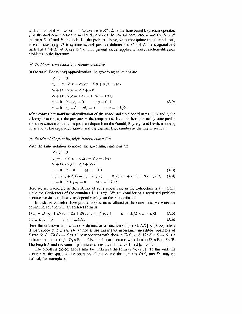
with x = x\ and y = x2 or y = (x2, x3); u e RN, Á is the transversal Laplacian operator, / is the nonlinear reaction term that depends on the control parameter \x and the N x N matrices D, C and E are such that the problem above, with appropriate initial conditions, is well posed (e.g. D is symmetric and positive definite and C and E are diagonal and such that C2 + E2 ^ 0, see [57]). This general model applies to most reaction-diflusion problems in the literature.
(b) 2D binary convection in a slender container
In the usual Boussinesq approximation the governing equations are
V -v = 0
vt + (v • V)v = aAv — Vp + a (9 — c)e2
6, + (v • V)<9 = A0 + Rv2
ct + (v • V)c = XAc + sXA6 - sRv2
v = 0 9 = cy=0 at y = 0, 1 (A.2)
v = 0 cx = 0 ± y6x = 0 at x = ±L/2.
After convenient nondimensionalization of the space and time coordinates, x, y and í, the velocity v = (v\, v2), the pressure p, the temperature deviation from the steady state profile 6 and the concentration c, the problem depends on the Prandtl, Rayleigh and Lewis numbers, a, R and X, the separation ratio s and the thermal Biot number at the lateral wall, y.
(c) Restricted 3D puré Rayleigh-Benard convection
With the same notation as above, the governing equations are
V -v = 0
vt + (v • V)v = aAv — Vp + a0e2
0t + (v • V)<9 = A0 + Rv2
v = 0 e = 0 at y = 0, 1 (A.3)
v(x,y,z + £,t) = v(x,y,z,t) 6(x, y, z + £, t) = 6(x, y, z, t) (A.4)
v = 0 0 ± y0x = 0 at x = ±L/2.
Here we are interested in the stability of rolls whose size in the z-direction is i = 0(1), while the slendemess of the container L is large. We are considering a restricted problem because we do not allow i to depend weakly on the x-coordinate.
In order to consider those problems (and many others) at the same time, we write the governing equations in an abstract form as
D0ut = Diuxx + D2ux + Cu + B(u, ux) + f(u, /x) in - L/2 < x < L/2 (A.5)
Cu ± Eux = O at x = ±L/2. (A.6)
Here the unknown u = u(x, t) is defined as a function of [—L/2, L/2] x [O, oo[ into a Hilbert space S, D0, Du D2, C and E are linear (not necessanly invertible) operators of S into S; C : V(C) -* S is a linear operator with domain V(C) cS,B:SxS^Sisa bilinear operator and / : V\ x R -+ S is a nonlinear operator, with domain V\xR c SxR. The length L and the control parameter \x are such that L ^> 1 and \\x\ <-¿ 1.
The problems (a)-(c) above may be written in the form (2.5), (2.6). To this end, the variable u, the space S, the operators C and B and the domains V(C) and T>\ may be defined, for example, as
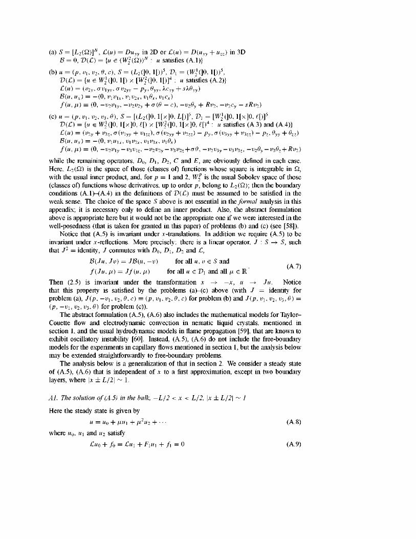
(a) S = [L2(£2)]N, C{u) = Duyy in 2D or C{u) = D{uyy + uzz) in 3D B = 0, V(C) = {ue (W2(í2)f : u satisfies (A.l)}
(b) u = (p, vu V2, 9, c), S = (L2(]0, 1[))5, V1 = (W¡(]0, 1[))5, V(C) = {u e W¡(]0, 1[) x [W¡(\0, 1[)]4 : u satisfies (A.2)} C(U) = (V2y, CíVlyy, aV2yy ~ Py , Oyy, XCyy + Sk9yy)
B(u, ux) = - (0 , vxvlx, vxv2x, vx6x, vxcx) f(u, /x) = (0, -v2v\y, -v2v2y + a (9 - c), -v29y + Rv2, -v2cy - sRv2)
(c) u = (p, Vl, V2, vs, 9), S = [(L2(]0, l[x]0, L[)]5, V1 = [W¡Q0, l[x]0, l[)]5
V{£) = {u e W¡Q0, l[x]0, í[) x [W¡{]0, l[x]0, l[)4 : u satisfies (A.3) and (A.4)} C{ü) = (V2y + V3z, a{Vlyy + V^), Cj{V2yy + V2zZ) ~ Py,a(V3yy + V3zZ ) ~ ft , Oyy + 6^)
B(u, ux) = - (0 , v\u\x, viv2x, viv3x, v\0x) f(u,[z) = (0, -v2v\y-v3vu, -v2v2y-v3v2z+a&, -v2v3y-v3v3z, -v26y-v3ez + Rv2)
while the remaining operators, D0, D\, D2, C and E, are obviously defined in each case. Here, L2 (Í2) is the space of those (classes oí) functions whose square is integrable in Í2, with the usual inner product, and, for p = 1 and 2, W% is the usual Sobolev space of those (classes of) functions whose derivatives, up to order p, belong to L2(Q); then the boundary conditions (A.1)-(A.4) in the definitions of V(C) must be assumed to be satisfied in the weak sense. The choice of the space S above is not essential in the formal analysis in this appendix; it is necessary only to define an inner product. Also, the abstract formulation above is appropriate here but it would not be the appropriate one if we were interested in the well-posedness (that is taken for granted in this paper) of problems (b) and (c) (see [58]).
Notice that (A. 5) is invariant under x-translations. In addition we require (A. 5) to be invariant under x-reflections. More precisely: there is a linear operator, / : S -+ S, such that J2 = identity, / conmutes with D0, D\, D2 and C,
BUu, Jv) = JB(u, —v) for all u, v e S and (A.7)
f(Ju, fi) = Jf(u, fi) for all u e T>\ and all ¡i. e R
Then (2.5) is invariant under the transformation x —>- — x, u -* Ju. Notice that this property is satisfied by the problems (a)-(c) above (with / = identity for problem (a), J(p, -vu v2, 9, c) = (p, vu v2, 9, c) forproblem (b) and J(p, vu v2, v3, 9) = (p, —v\, v2, v3, 9) for problem (c)).
The abstract formulation (A.5), (A.6) also includes the mathematical models for Taylor-Couette flow and electrodynamic convection in nematic liquid crystals, mentioned in section 1, and the usual hydrodynamic models in llame propagation [59], that are known to exhibit oscillatory instability [60]. Instead, (A.5), (A.6) do not include the free-boundary models for the experiments in capillary flows mentioned in section 1, but the analysis below may be extended straightforwardly to free-boundary problems.
The analysis below is a generalization of that in section 2. We consider a steady state of (A.5), (A.6) that is independent of x to a first approximation, except in two boundary layers, where |x ± L/2\ ~ 1.
Al. The solution of (A.5) in the bulk, —L/2 < x < L/2, |x ± L/2\ ~ 1
Here the steady state is given by
U = Wo + /¿U\ + fl u2 + • • •
where u0, u\ and u2 satisfy
-C«o + /o = £wi + FiUi + fi = 0
(A.8)
(A.9)
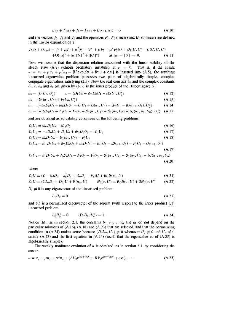
Cu2 + Fxu2 + f2 + F2ux + Bi(«i, ux) = O (A.10)
and the vectors f0, fx and f2 and the operators Fx, F2 (linear) and Bx (bilinear) are defined in the Taylor expansión of /
f(u0 + U,fi) = f0 + /x/i + fi2f2 + (Fx + fiF2 + fi2F3)U + Bx (U, U) + C(U, U, U)
+0(|/x|3 + |/x|||C7||2+||C7||4) as \i¿\ + \\U\\ - + 0 . (A. 11)
Now we assume that the dispersión relation associated with the linear stability of the steady state (A. 8) exhibits oscillatory instability at \x = 0. That is, if the ansatz u = u{) + ixu\ + ix2u2 + [£/exp(£2í + ikx) + c e ] is inserted into (A.5), the resulting linearized eigenvalue problem possesses two pairs of algebraically simple, complex conjúgate eigenvalues satisfying (2.5). Now the real constant b0 and the complex constants b\, c, do and d\ are given by ((•, •> is the inner product of the Hilbert space S)
b0 = {CiUo, UZ) c = {DxUo + iboDoUx - iCxUx, W0) (A. 12)
do = {B2(Ul, Uo) + F2U0, UZ) (A.13)
bx = {-b0D0U3 + idoDoU, + £ , [ / 3 + B(Ul, Uo) - iF2Ux - iB2(Ul, Ux), U^) (A. 14)
dx = {-d0D0U3 + F3U0 + F2U3 + B2(uu U3) + B2(u2, U0) + 3C(m, uu U0), U^) (A. 15)
and are obtained as solvability conditions of the following problems
CoU^iboDoUo-iCiUo (A. 16)
C0U2 = -cD0Uo + DxUo + \boDoUx - iCxUx (A. 17)
C0U3 = doDoUo - B2(ux,Uo) - F2U0 (A. 18)
C0U4 = ibxD0U0 + ib0D0U3 + d0D0Ux - iCxU3 - iB(ux, U0) - F2UX - B2(ux,Ux)
(A. 19)
C0U5 = dxD0U0 + d0D0U3 - F3U0 - F2U3 - B2(ux, U3) - B2(u2, U0) - 3C(ux, ux,U0)
(A.20)
where
C0U = {C- icoDo - klDx + ik0D2 + FX)U + ik0B(u0, U) (A.21)
CXU = (2ik0Dx +D2)U +B(u0,U) B2(u,U) = ik0B(u,U)+ 2Bx(u,U) (A.22)
Uo T¿ 0 is any eigenvector of the linearized problem
£0Uo = 0 (A.23)
and U¿ is a normalized eigenvector of the adjoint (with respect to the inner product (, » linearized problem
CIU* = 0 (DoUo, U*) = 1. (A.24)
Notice that, as in section 2.1, the constants b0, bx, c, d0 and dx do not depend on the particular solutions of (A. 16), (A. 18) and (A.23) that are selected, and that the normalizing condition in (A.24) makes sense because (D0U0, Ufi) ^ 0 whenever U0 =£ 0 and UQ ^ 0 satisfy (A.23) and the first equation in (A.24) (recall that the eigenvalue ico of (A.23) is algebraically simple).
The weakly nonlinear evolution of u is obtained, as in section 2.1, by considering the ansatz
Uo + IJMX + IJ,2U2 + {AUoéCút+lkQX + BVoé0"-^1 + ce.) + • • • (A.25)

where the complex amplitudes are small and depend weakly on x and t. The evolution equations for A and B are obtained, as in section 2.1, to be given again by (2.16), (2.17), while U is given by
u = u0 + ixui + ¡J2U2 + [(AUo - iAx(Ui + i¿U4) - AXXU2 + f¿A(U3 + ixU5)
+A\A\2Ug + A\B\2U9 + HORTl)eia>í+I*°x + c e ]
+[(BV0 + iBx(V1+/xV4)-BxxV2 + /xB(V3+/xV5) + B\B\2Vs
+fí|A|2V9 + HORT2)eia>í^0X + c e ]
+[(A2U6e2lk°x + B2V6e-2lkoX)e2wt + ABW^210* + ABW2e
2lk°x + c e ]
+ \A\2U7+ |fí|2V7+HONRT (A.250
where HONRT, HORT1 and HORT2 are as in (2.19), (2.20) and, the vectors U0,...,U5
are as obtained above, while the remaining vectors are given by
(£„ + C22)U6 = -ik0B(U0, U0) - Bl (Uo, U0) (A.26)
(£o + £oo)U7 = ik0B(U0, Ü0) - B2(Ü0, U0) (A.27)
(£o + £20)Wj = ik0B(U0, V0) - B2(V0, U0) (A.28)
(£0 + £02)^2 = -ik0B(U0, Vo) - ik0B(V0, U0) - 2B,(V0, U0) (A.29)
£0C/8 = eiD0Uo - B2(U7, Uo) - B3(U6, Ü0) - 3C(U0, U0, Ü0) (A.30)
C0U9 = e2D0U0 - B2(V7, U0) - B2(WU V0) - B3(W2, V0) - 6C(U0, V0, %) (A.31)
Vj = JUj for j = 0 , . . . , 9 (A.32)
where the linear operators / , £0 and £ r s for r,s = 0, 2, and the bilinear operators B2 and B3 are given by (A.6), (A.21), (A.22) and
£ „ = [i(l - r)eoD0 + (1 - s2)k2D, + i(j - l)k0D2]U + i(j - l)koB(uo, U) (A.33)
B2(U, V) = ik0B(U, V) +2B1(U, V) (A.34)
B3(U, V) = B2(U, V) +2ik0[B(V, U) - B(U, V)]. (A.35)
As in section 2.1, U6, U7, W\ and W2 are uniquely determined by (A.26)-(A.29), while (A.30) and (A.31) possess a solution if and only if
ex = {B2(U7, Uo) + B3(U6, Ü0) - 3C(U0, U0, Ü0), U^} (A.36)
e2 = {B2(V7, Uo) + B2(WU Vo) + B3(W2, V0) + 6C(U0, V0, V0), U¿} (A.37)
and this determines the coefficients e\ and e2 of (2.14), (2.15).
A2. The solution of (A.5), (A.6) in the boundary layers, \x ± L/2\ ~ 1
As in section 2.2 we consider only the boundary layer near x = —L/2 and use the re-scaled coordinate
f = x + L/2. (A.38)
The steady state in this boundary layer is
u = u°(í;) + iiul (£) + ••• (A.39)
where ul and u2 satisfy
DlU0^ + D2u\ + £w° + B(u°, u¡) + / ° ( f ) = 0 (A.40)
C°ul + f (f) = 0 in 0 < f < 00 (A.41)
Cu0 - Eu\ = Cul -Eu\=Q at f = 0 (A.42)
u° -+ u0 ul -* u\ as f —>- 00 (A.43)

Here w0 and u\ are given by (A.9), (A. 10), the linear operator £° is given by
£°u = A % + D2u% + [£ + Fl(f )]w + ¿3(w°, ¡ÍJ) + B(u, u¡) (A.44)
and, for each f, the vectors / ° and Z1 and the linear operator F 1 are defined in the Taylor expansión of / around u = u°, \x = 0,
/(«°(f) + C/, /x) = / ° + l¿f + (í^1 + M^ 2 )^ + &(U, U) + C\U,U,U) + ---. (A.45)
The multihnear operators Bl and C1 will be used below and depend also on f. Notice that if (A.43) holds then
/ " - • / o / ' - • / i F 1 ^ ^ F 2 ^ F 2 , , (A.46)
¿31 - ^ 6 , aad C U C as £ -> oo
where /0 , / i , F\, F2, B\ and C are defined in the Taylor expansión (A. 11). We assume that (A.40), (A.42), (A.43) has a unique solution; this assumption must be
analysed carefully in each particular case since it does not need to hold in semi-infinite multidimensional nonlinear problems, even for the simplest reaction-diffusion equations [60,61]. We also assume that the linearized problem
£°U = QD0U in 0 < f < oo (A.47)
CU-EU¡:=0 a t f = 0 \\U\\ boundedasf -> oo (A.48)
has a nontrivial eigenfunction, U°, associated with the eigenvalue ico, that satisfies
£°U° = icoD0U° in 0 < f < oo (A.49)
CU°-EU¡ = 0 a t f = 0 || £7° || bounded as f -^ oo (A.50)
and that the remaining part of the spectram has a negative real part and lies at a non-zero distance from any point of the imaginary axis different from ±ico. Then (Í2 = 0 does not belong to the spectram of (A.47), (A.48) and) (A.41)-(A.43) uniquely determines ul. Finally, we assume that the convergence in(A.43) is exponential, and that there is a complex constató r\ ^ 0 such that the eigetóunctions of (A.49), (A.50) satisfy
||C/°(f) - U0Qlk^ - n Voe"1*^ || -^ 0 exponentially as f -^ oo. (A.51)
These are again nontrivial issues for semi-infinite multidimensional problems, specially in the nonlinear case [63,64]. Fortunately, the assumptions made above about the spectram of (A.47), (A.48) imply that the convergence (A.43) is exponential; this may be proven by applying classical general results in [65,66] for the linear case, and those in [67] for the nonlinear case. The assumption (A.51) instead must be analysed in each particular case. Notice that our assumptions imply that the convergence in (A.46) is also exponential.
Under the assumptions above, the weakly nonlinear evolution of the solutions of (A. 5), (A.6) in this boundary layer is given by
u =u° + /.M1 + [(aU° + afiU1 + a\a\2U4 + atU5 + HORT)ela>í + a2U2e2wt + c e ]
+ |a|2C73+HONRT (A.52)
where HORT and HONRT are as in (2.34), the complex amplitude a is small and depends weakly on time, U° =¿= O is given by (A.49), (A.50) and U1,..., U5 are now given by
C°Ul - icoDoU1 = -F2U° - 2B2(u\U°) (A.53)
£°U2 - 2icoD0U2 = -B2(U°, U°) (A.54)
C°U3 = -2B2(U°, Ü°) (A.55)
C°U4 - ÍOJDQU4 = -2B2(Ü°, U2) - 2B2(U°, U3) - 3C\U°, U°, Ü°) (A.56)
1164 C Martel andJMVega
CU — icoDoU = Dolí in O < f < oo (A.57)
CU' — EUí = O at f = 0 (A.58)
U' diverges at most algebraically as f -> oo (A.59)
for j = 1 , . . . , 5. The Minear operator B2 is given by
B (U, V) = —IB (U, V) — B(U, Vx) — B(V, Ux)
and the operators F2 and C1 are defined in (A.45). For matching purposes we only need the asymptotic behaviour of Ul,..., U5 at f = oo. When taking into account that the convergence is exponential in (A.43), (A.46) and (A.51), it is seen that
Ul = [b^ldo(—^Uo + iU\) + U^e1 "^ + r\ [b^ldo(^Vo + iVi) + V^e-1 °̂ + EST (A.60)
U2 = U(,Q2lki>'^ + r2Vse^2lk"^ + r\ W\ + EST (A.61)
U3 = f\ W2e2lk"^ + c.c. + U-¡ + \r2 \ V-¡ + EST (A.62)
U4 = [b-l{ei + \rl\2e2)(-l;Uo + iUl) + Us + |r1|
2C79]e1^
+ri[^o^1(eilri |2 + ei)(% Vo + i Vi) + \r\ |2 Vg + Vgje-1*0^ +EST (A.63)
U5 = by1 (í; UQ — iUi)elko!¡ + ribyl(—í;Vo — iVOe-1*0^ + EST (A.64)
where the vectors TJ¡, V, (for j = 0 , . . . , 9), W\ and W2 are solutions of (A.16)-(A.20), (A.23) and (A.26)-(A.32), the constants bo, c, do, e\ and e2 are given by (A.12), (A.13) and (A.36), (A.37), and EST stand for exponentially small terms as f -> oo.
A3. Matching between the solutions in the bulk and in the boundary layers
As in section 2.3 we apply matching conditions between the solutions in the bulk and in the boundary layer at x = —L/2, to obtain the boundary conditions to be applied to the solutions in the bulk. To this end we write the solutions in the bulk and in the boundary layer in terms of the variable (A.38) and consider the limit
1 <C f <C A (A.65)
where A. is as in section 2.3. The solution in the bulk is obtained by replacing (A.38) into (A.25’) to obtain
u = [(Ao + AQX^)U() — iAoxí7i — A()XXU2 + ¡I-AQUI,
+A0(\A0\2Ug + \B0\
2U9) +HOR^l]éa't+lkol;-lkoL,2
+[(B0 + BoxHWo + i#oxVi - B0xxV2 + /¿B0V3
+Bo(\Bo\2Vg + | Ao|2 V9) + HORT2]eia>í~1*0^+1*°L/2 +c.c. +NRT (A.66)
and the solution in the boundary layer is obtained by placing (A.51) and (A.60)-(A.64) into (A.52), to give
u = [aUo + b~Q (at — do/j,a — {e\ + \r\ \ e2)a\a\ )(f UQ, — iU\) + ayuUj,
+a\a\2(Ug + \n \2U9) + HORT]ela>í+I^
+ri[aVo + b~Q (—at + do/j,a + {e\ + \r\ \ e2)a\a\ )(f Vo + i Vi) + ajxV^
+a\a\2(\ri\2Vg + V9) + HORT]ela>í_I^ (A.67)
where HORT1, HORT2, HORT and NRT, Ao, fio, ^ox and BQ,X are as in (2.56), (2.57). Then, by identifying (A.66) and (A.67) we obtain (2.58), (2.59) again. As a consequence, (2.61) holds and the derivation of the boundary conditions at x = —L/2 is complete. The boundary conditions (2.63) are obtained in a completely similar way.
Appendix B. Large time behaviour of the solutions of the linear system (5.27)-(5.31)
Here we obtain sufficient conditions for properties 1 and 2 in section 5.1 to hold; more general conditions are omitted for the sake of brevity and will be considered elsewhere [44]. To proceed we first apply a reflection principie at f = ±1/2 to rewrite (5.27)-(5.31) as
UkT -Utt: = -(k2 + 2f)Uk + a2k2 Vk (B. 1)
VkT ~ Vkf = -(a2k2 + 2a3f)Uk - k2Vk (B.2)
UkG + 2,T) = Ukg,T) VkG + 2,T) = Vkg,T) i n - o o < f < o o (B.3)
Uk(M, 0) = Um(£) Vk(^, 0) = Vt0(£) (B.4)
where
U&, T) = «+(£, T)
V*(£, T) = u+(£, T)
f^,T) = \Y0(^,T)\2 if - 1/2 < £ < 1/2 (B.5)
UkG,T) = Ut(-l-Z,T)
vt(f,r) = wt-(-i-f,r) / (£ , r ) = | Z 0 ( - l - f , T)|2 if - 3 / 2 < f < - l / 2 (B.6)
/ (£ + 2 , r ) = / ( £ , r ) i f - o o < f < o o . (B.7)
Equations (5.10)-(5.12) and (B.5)-(B.7) imply that if p = 1 then the function / is smooth in— o o < f < o o , 0 < r < o o , while if p =/= 1 then / is only piecewise smooth (it is discontinuous at f = 1/2 + m for each integer m and each T > 0); then some care must be taken below when obtaining general properties concerning the asymptotic behaviour of Uk and Vk as T -+ oo. Also, as was seen in section 5.2, in the supercritical case, a\ > - 1 , | Y01 and |Z0| are uniformly bounded above in - 1 / 2 < f < 1/2 for all T > 0. In some cases (e.g. when analysing solutions of (5.10)-(5.12) that converge to either a steady state or a limit cycle as T -+ oo), | Y0 \ and | Z01 are also uniformly bounded below by a strictly positive constant as T ->- oo. Then we shall assume that / > 0 is uniformly bounded above in -oo < f < oo for all T > 0; also, we shall consider the case when / is uniformly bounded below by a strictly positive constant, in -oo < f < oo, for all T > 0.
Notice that when using the characteristic variable
n = T-H (B.8)
equations (B.1)-(B.4) are reduced to the following pair of ODEs:
Ukn = -{k2 + 2f)Uk + a2k2 Vk (B.9)
Vkn = -{a2k2 + 2a3f)Uk - k2Vk (BAO)
UkG,-Z) = Uk0G) Vt(f, - f ) = Vto(É) (B.H)
where the variable f acts as a parameter and
/(f, ÍJ) = / (£ , f + ÍJ).
Notice also that since Uk and Vk satisfy the periodicity conditions (B.3), in order to obtain asymptotic bounds as T -+ oo, that are uniformly valid in -oo < f < oo, we only need to obtain bounds valid in one period, e.g. in 0 < f < 2.
If |iol and |Zol are constant (this requires the boundaries to be perfectly reflecting, i.e. p to be equal to 1, see (5.10)-(5.12)), then the function / is constant (see (B.5), (B.6)) and
the solutions of (B.9), (B.IO) are readily obtained in closed form. Then the folio wing result applies.
Lemma B.l. Let f > 0 be a constant. If\+ a2a3 > 0 then every solution of(B.9), (B.IO) satisfies
|£4I +I VtK^oexpt-M (£)?]]
where KQ, is a constant depending on the initial conditions, Xi(k) = (k2 + f) if p(k) = f2-2a2a3k
2f-ajk4 < 0 and X^k) = [2(1 + a2a3)f + (1 + a¡)k2]k2 / (k2 + f + ^pW)) otherwise. Lf\ + 0(20(3 < 0 and p(k) > 0 then there is a solution of (B.9), (B.IO) such that
\Uk\ + \Vk\^K{)QW[X2{k)V]
where X2(k) = [2(1 + a2a3)f + (1 + a2)k2]k2/((k2 + f) - JpW)) > 0.
Proof. The result follows when solving (B.9), (B.IO) in closed-form.
Lemma B.2. Let f be a piecewise smooth, positive function, and let the constants a2 and a3 be such that — 1 < a2a3 < 1. Then, every solution of (B.l)-(BA) satisfies
|£4I + IVtK K0exp(-Xk2T) as T -> 00
for all h,, where the constant K0 depends on the initial conditions (B.4) and
X = 1 + oi2a3 if — 1 < a2a3 ^ 0 A. = 1 — a2a3 ifO < a2a3 < 1.
Proof. If a2 = 0 then the result readily follows from (B.9), (B.IO). If a2 ,é 0 then we introduce the new dependent variable
Wk = a2(a3Uk - Vk) exp[(l + a2a3)k2r]] (B.12)
to reduce (B.9)-(B.ll) to
Wkm + 2 ( / - a2a3k2)Wkn + a\{\ + aj)k4Wk = 0 (B.13)
W¡t(£, -£ ) = a2[a3Uk0G) - Vt0(f)] exp[-(l + a2a3)k2^] (B.14)
Wkr¡(^, - £ ) = a\{\ + a23)k
2Uk0^)exp[-(l +a2a3)k2^]. (B.15)
Notice that
a\{\ + aj)k2Uk = Wkn exp[-(l + a2a3)k2r¡] (B.16)
a22(l + af)k2Vk = [a3Wkn - a2(l + aj)k2Wk]exp[-(l + a2a3)k
2r¡]. (B.17)
Now, when multiplying (B.13) by Wkr} and integrating in ] - f, r¡[ we obtain
W2kl] + aj(l + a¡)k4W2 < Kx + 4 f (a2a3k
2 - f)W2kr] di] (B.18)
J—%
if 0 < f < 2 and ?j > —f, where
Kx = a4{\ + aj)k4 max{(l + aj)Uk0^)2 + [a3Uk0& - Vk0(^)]2}.
If - 1 < a2a3 < 0 then W2n + a2(1 + a2)£4W2 < K¡ (see (B.18)) and the result readily
follows when taking into account (B.16), (B.17). If 0 < a2a3 < 1 then by applying Gronwall's lemma to (B.18) we obtain
W¡n < Ki exp[4a2a3k2(r¡ + H)] < Kx exp[4a2a3k
2 (r¡ + 2)]
if 0 < f < 2 and ?j > —f; when taking into account (B.16), (B.17) the result follows again, and the proof is complete.
Lemma B.3. Let f be uniformly bounded above and satisfy the assumptions in lemma B.2, and let the constant F* be given by
i n ~ i rT
F* = sup l imsup- / /(f, z)dz = sup limsup — / /(f, z)dz.
In, addition
a2a3 ^ 1 and k2 > pF* with p = va2 + 1 — 1.
then every solution of(B.l)—(B.4) satisfies
\Uk\ + \Vk\^K0exp[(pF*-k2)T] as T -* oo
for all í¡, where the constant KQ, depends on the initial conditions.
Proof. We introduce the new dependent variable
Wk = Ukexp(2F+k2r¡) with F(£, r¡) = í / (£ , z)dz (B.19)
to write (B.9), (B.10) as
Wt,, - 2/Wt, + (a22¿4 + 2a2a3/*2)W¡t = 0. (B.20)
Notice that Uk and V¿ may be obtained in terms of Wk and Wkj] by means of (B.19) and
Wkri = a2k2VkQxp(2F + k2r]). (B.21)
Now, we multiply (B.20) by Wkj] exp(-4F), intégrate in ] - f,)][ and intégrate by parts to obtain
(Wl„ + ajk4W2) exp(-4F) < Kx - \a\k4 f / (£ , z)Wk(¿, zf exp[-4F(f, z)] dz
-4a2a3k2 í /(f,z)W¡t(f, 2 ) ^ , ( 1 , z)exp[-4F(f,z)]dz (B.22)
where the constant í^ depends on the initial conditions. But, by Cauchy's inequality we have, for all X > O,
"i \a2a3k
2 i" fG,z)WkG,z)WknG,z)exp[-4Fg,z)]dz
< 2 a 2 a 3 1 ' / (£ , z)[U4W t(f, zf + k^W^, z)2]exp[-4F(f, z)]áz.
If we select here
k = (a2/a3) (l + Vi + a2)
(the positive root of a3k2 - 2a2X — a\a3 = 0) and substitute in (B.22) we obtain
{W2V + ajk4W2) exp(-4F) < Kx + {2a2a3/X) f / (£ , z)[Wk^, zf + a¡k4Wk(^, zf]
J-l;
xexp[-4F(f ,z)]dz
and, by applying Gronwall's inequality
exp(-4F)(W£, + axk4W¡) < K2exp(2a2a3F/X)
for a certain constant K2 depending on initial conditions. When taking into account (B.19) and (B.21) the result follows, and the proof is complete.
Lemma B.4. Let f be uniformly bounded below by a positive constant and satisfy the assumptions in lemma B.3, and let the constants f and f* be given by
f = inf liminf / (£ , n) = inf liminf / (£ , T) 0<£<2 í)-*-oo 0<£<2 T^oo
/* = sup limsup/Xf, r¡) = sup limsup/Xf, T). 0<£<2 I J ^ O O 0<£<2 T-?oo
Ifa^a3 < — 1, thenfor each k and each p > O satisfying
k2 < -2(1 + aiQ!3)/+/(l + a22) (B.23;
/x < - ( ¿ 2 + /*) + V(k2 + f*f - 2(1 + a2a3)k2f - (1 + a¡)k4 (B.24)
there is a solution of(B.l)—(B.4) and a constant T0 such that
\Uk\ + \Vk\ ^ expQiT) ifT> T0and^ e R.
Proof. Let the constants f\ and f2 be such that
- ( 1 + a22)k
2/2{\ + a2a3) < A < f f < f2 (B.25)
p = -(k2 + f2) + j{k2 + f2f - 2(1 + a2a3)fx - (1 + a¡)k4. (B.26)
Such constants exist because k and /x satisfy (B.23), (B.24) and the right-hand side of (B.26) decreases whenever (B.25) holds and either f\ decreases or f2 increases (and it vanishes as /i = - ( 1 + aj)k2/2(1 + a2a3)). Also, (B.25) and the definition of /* and / * imply that there is a constant r¡0 such that
/i < /(£,»?) < fi if O % for all £. (B.27)
Now, let us introduce the new variable
Wk = a2(a3Uk - Vk) exp(-prj) (B.28)
to write (B.9), (B.10) as (see (B.26))
Wkm + 2(p + k2 + f)Wkn + [2p(f - f2) + 2(1 + a2a3)k2(f - fi)]Wk = O (B.29)
and, for each f e [-2, 0], consider the solution of (B.29) such that
Wk = max{\a2a3\, \a2\] Wkr¡ = O at r¡ = r¡0. (B.30)
That solution increases as r¡ (> r¡0) increases because, since the coefficient of Wk in (B.29) is negative (see (B.27)), Wkj]J] > O at r¡ = r¡0, and Wk cannot have a local máximum if r] > r¡o. Then if - 2 < f < O and T > r¡0 + 2 we have (see (B.8) and (B.28))
\Uk\ + Wk\> \Wk\/max{\a2a3\, \a2\] > exp(prj) > exp(pT)
and the result follows. Thus the proof is complete.
When collecting the results in lemmas B.1-B.4 and taking into account (B.5)-(B.8), the following result is obtained.
Theorem B.5. (a) If either (i) — 1 < a2a3 < 1, or (ii) a2a3 ^ 1 and k is not too small, or (iii) a2a3 ^ —1 andboth |io| ond |Zo| are constant, thenproperty 1 ofsection 5.1 applies.
(b) If'a2a3 < — 1 and both \Y0\ and \Z0\ are uniformly bounded below by a strictly positive constant as T -> oo, then property 2 ofsection 5.1 applies.

References
[i
p;
[3
[4:
[5
[7
[«
[9
[ío;
[11
[12;
[13
[14;
[15
[ie;
[17;
[1
[19; [20 [21
[22;
[23
[24
[25
[26
[27
[28 [29
[30
[31
Cross M C and Hohenberg P C 1993 Pattern formation outside of equilibrium Rev. Mod. Phys. 65 851-1112 Steinberg V, Fineberg J, Moses E and Rehberg I 1989 Pattern selection and transition to turbulence in
propagating waves Physica 37D 359-83 Bensimon D, Kolodner P, Surko C M, Williams H and Croquette V 1990 Competing and coexisting dynamical
states of travelling-wave convection in an annulus J. Fluid Mech. 217 441-67 Kolodner P 1993 Repeated transients of weakly nonlinear travelling-wave convection Phys. Rev. E 47 1038-
48 Kaplan E and Steinberg V 1993 Measurement of reflection of travelling waves nearthe onset of binary-fluid
convection Phys. Rev. E 48 R661^1 Predtechensky A A, McCormick W D, Swift J B, Noszticzius Z and Swinney H L 1994 Onset of travelling
waves in isothermal double diffusive convection Phys. Rev. Lett. 72 218-21 Motsay R W, Anderson K E and Behringer R P 1988 The onset of convection and turbulence in rectangular
layers of normal liquid 4He J. Fluid Mech. 189 263-86 Croquette V and Williams H 1989 Nonlinear competition between waves on convective rolls Phys. Rev. A
39 2765-8 Croquette V and Williams H 1989 Nonlinear waves of the oscillatory instability on finite convective rolls
Physica 37D 300-14 Andereck C D, Liu S S and Swinney H L 1986 Flow regimes in a circular Couette system with independently
rotating cylinders J. Fluid Mech. 164 155-83 Tagg R, Edwards W S and Swinney H L 1990 Convective versus absolute instability in flow between
counter-rotating cylinders Phys. Rev. A 42 831-7 Dubois M, Daviaud F, Ronsin O and Bergé P 1992 Traveling waves in puré fluids locally heated along wires
Physica 61D 140-6 Vince J M and Dubois M 1992 Hot wire below the free surface of a liquid: structural and dynamical
properties of a secondary instability Europhys. Lett. 20 505-10 Daviaud F and Vince J M 1993 Travelling waves in a fluid layer subjected to a horizontal temperature
gradient Phys. Rev. E 48 4432-6 Joets A and Ribotta R 1988 Localized, time-dependent state in the convection of a nematic liquid crystal
Phys. Rev. Lett. 60 2164-7 Rehberg I, Rasenat S and Steinberg V 1989 Travelling waves and defect-initiated turbulence in
electroconvecting nematics Phys. Rev. Lett. 62 756-9 Rehberg I, Winkler B L, de la Torre M, Rasenat S and Schópf W 1989 Pattern formation in a liquid crystal
Advances in Solid State Physics vol 29, ed V Roessler (Braunschweig: Vieweg) pp 35-52 de la Torre M 1990 Contribución al estudio de la formación de estructuras en fluidos anisótropos Doctoral
Thesis Universidad Nacional de Educación a Distancia, Madrid Markstein G H 1964 Nonsteady Fíame Propagation (New York: Plenum) Ferguson C R and Keck J C 1979 Stand-off distances on a flat burner Combustión and Fíame 34 85-98 Sabathier F, Boyer L and Clavin P 1979 Experimental study of weak turbulent premixed flames Combustión
andFlame 35 139-53 Buckmaster J 1983 Stability of the porous plug burner llame SIAM J. Appl. Math. 43 1335^19 Margolis S B and Williams F A 1989 Diffusional-thermal instability of a solid propellant fíame SIAM J.
Appl. Math. 49 1390^120 Coullet P, Fauve S and Tirapegui E 1985 Large scale instability of nonlinear standing waves J. Physique
Lett. 46 787-91 Hohenberg P C and Cross M C 1987 An introduction to pattern formation in non-equilibrium systems Lecture
Notes in Physics vol 268 (Berlin: Springer) Fauve S 1987 Large scale instabilities of cellular flows Instabilities and Non-equilibrium Structures ed E
Tirapegui and D Villarroel (Dordrecht: Reidel) Pierce R D and Knobloch E 1995 Asymptotically exact Zakharov equations and the stability of water waves
with bimodal spectra Physica 81D 341-73 Christodoulides P and Dias F 1994 Resonant capillary-gravity interfacial waves J. Fluid Mech. 265 303-43 Nicolás J A, Martel C and Vega J M 1996 Weakly non-linear oscillations in liquid bridges under high-
frequency axial forcing in preparation Knobloch E and Gibbon J D 1991 Coupled NLS equations for counter propagating waves in systems with
reflection symmetry Phys. Lett. 154A 353-6 Cross M C 1986 Travelling and standing waves in binary-fluid convection in finite geometries Phys. Rev.
Lett. 57 2935-8

[32] Cross M C 1988 Structure of nonlinear travelling waves in finite geometries Phys. Rev. A 38 3593-600 [33] Cross M C 1989 Nonlinear travelling wave states in finite geometries Physica 37D 315-8 [34] Cross M C and Kuo E Y 1992 One dimensional spatial structure near a Hopf bifurcation at finite wave
number Physica 59D 90-120 [35] Bensimon D, Kolodner P, Surko C M, Williams H and Croquette V 1990 Competing and coexisting dynamical
states of travelling-wave convection in an annulus J. Fluid Mech. 217 441-67 [36] Chikwendu S C and Kevorkian J 1972 A perturbation method for hyperbolic equations with small
nonlinearities SIAM J. Appl. Math. 22 235-58 [37] Knobloch E and de Luca J 1990 Amplitude equations for travelling wave convection Nonlinearity 3 575-80 [38] Alvarez-Pereira C and Vega J M 1992 On the pulsating instability of two-dimensional llames Eur. J. Appl.
Math. 3 55-73 [39] Vega J M 1993 On the amplitude equations arising at the onset of the oscillatory instability in pattern
formation SIAM J. Math. Anal. 24 603-17 [40] Knobloch E 1992 Nonlocal amplitude equations Pattern Formation in Complex Dissipative Systems ed S Kai
(Singapore: World Scientific) [41] Martel C 1995 La Inestabilidad Oscilatoria y sus Aplicaciones en Mecánica de Fluidos y Combustión Doctoral
Thesis Universidad Politécnica de Madrid, Madrid [42] Martel C and Vega J M 1996 A non-local amplitude equation that applies at the oscillatory instability in
finite geometries, in preparation [43] Martel C and Vega J M 1996 Global stability properties of a hyperbolic system arising in pattern formation
Nonlinear Anal. TMA to appear [44] Martel C and Vega J M 1996 Dynamics of a hyperbolic system that applies at the onset of the oscillatory
instability, in preparation [45] Knobloch E 1986 Oscillatory convection in binary mixtures Phys. Rev. A 34 1538^19 [46] Dangelmayr G and Knobloch E 1987 The Physics of Structure Formation: Theory and Simulation ed W
Güttinger and G Dangelmayr (Berlin: Springer) [47] Clever R M and Busse F H 1989 Nonlinear oscillatory convection in the presence of a vertical magnetic
field J. Fluid Mech. 201 507-23 [48] Schópf W and Zimmermann W 1989 Multicritical behaviour in binary fluid convection Europhys. Lett. 8
41-6 [49] Dangelmayr G, Knobloch E and Wegelin M 1991 Dynamics of travelling waves in finite containers Europhys.
Lett. 16 723-9 [50] Knobloch E and Silber M 1993 Oscillatory convection in a rotating layer Physica 63D 213-32 [51] Kevorkian J and Colé J D 1981 Perturbation Methods in Applied Mathematics (Berlin: Springer) [52] Lagerstrom P A 1988 Matched Asymptotic Expansions (Berlin: Springer) [53] Roberts A J 1992 Boundary conditions for approximate differential equations J. Austral. Math. Soc. Ser. B
34 54-80 [54] Jeffrey A and Kawahara T 1982 Asymptotic Methods in Nonlinear Wave Theory (Boston, MA: Pitman) [55] Coddington E A and Levinson N 1955 Theory of Ordinary Differential equations (New York: McGraw-Hill) [56] Gil L 1991 Space and time intermittency behaviour of a one-dimensional complex Ginzburg-Landau equation
Nonlinearity 4 1213-22 [57] Eidel'man S D 1969 Parabolic Systems (Amsterdam: North-Holland) [58] Teman R 1983 Navier-Stokes Equations and Nonlinear Functional Analysis (Society for Industrial and Applied
Mathematics) [59] Clavin P 1985 Dynamic behaviour of premixed flame fronts in laminar and turbulent flows Prog. Energy
Combust. Sci. 11 1-59 [60] Jackson T L and Kapila A K 1986 Thermal expansión effects on perturbed premixed llames Reacting Flows:
Combustión and Chemical Reactors (Lectures in Applied Mathematics 24-1) ed G S S Ludford (Providence, RI: American Mathematical Society) pp 325-48
[61] Parra I E and Vega J M 1992 Múltiple solutions of some semilinear elliptic equations in slender cylindrical domains J. Diff Eqns 100 225-56
[62] Dancer E N 1993 Weakly nonlinear Dirichlet problems on long or thin domains Mem. Am. Math. Soc. 105 501
[63] Berestycki H and Nirenberg L 1990 Some qualitative properties of solutions of semilinear elliptic equations in cylindrical domains Analysis ... etc, Research Papers Published in Honor of Jurgen Moser's 60th Birthday ed P H Rabinowitz and E Zehnder (New York: Academic) pp 115-64
[64] Vega J M 1993 The asymptotic behaviour of the solutions of some semilinear elliptic equations in cylindrical domains J. Diff. Eqns 102 119-52
[65] Agmon S and Nirenberg L 1963 Properties of solutions of ordinary differential equations in Banach space Commun. PureAppl. Math. 16 121-239
[66] Pazy A 1967 Asymptotic expansión of solutions of ordinary differential equations in Hilbert space Are. Rational Mech. Anal. 24 193-218
[67] Simón L 1985 Isolated singularity of extrema of geometric variational problems Harmonic Mappings and Minimal Immersions (Lecture Notes in Mathematics 1161) ed E Giusti (Berlin: Springer)