1

FINITE ELEMENT STUDY OF NERVE FIBERS AROUND RETINAL ARTERIES AND POSSIBLE RISK FACTORS FOR GLAUCOMA

By

DEVESH CHUGH

A THESIS PRESENTED TO THE GRADUATE SCHOOL OF THE UNIVERSITY OF FLORIDA IN PARTIAL FULFILLMENT

OF THE REQUIREMENTS FOR THE DEGREE OF MASTER OF SCIENCE

UNIVERSITY OF FLORIDA

2012

2

© 2012 Devesh Chugh

3

To my Parents

4

ACKNOWLEDGMENTS

It has been one of the toughest journeys of my life and I want to extend my

sincere thanks to all the people who have helped me in getting across the line. I want to

thank my advisor Dr. Roger Tran-Son-Tay who guided me all these two years. With him,

I have gained a research experience that is going to help me all my life. I also want to

thank Dr. Malisa Sarntinoranont and Dr. Nam Ho Kim for being on my committee and

always extending time and help whenever I faced a problem in my project.

I thank my friends in Gainesville who were like a family, always supporting me

away from my home. I also want to thank my friends back home in India who have

supported me throughout this time.

I want to thank my father and mother who have been constant source of love,

inspiration, motivation and guidance. I also want to thank for all the love, support and

care that I received from my sisters, brother in laws and my girlfriend Sakshi.

My master’s journey has contribution from all these people and this won’t have

been possible with the patience, support and motivation that these people have

extended to me.

5

TABLE OF CONTENTS Page

ACKNOWLEDGMENTS .................................................................................................. 4

LIST OF TABLES ............................................................................................................ 7

LIST OF FIGURES .......................................................................................................... 8

LIST OF ABBREVIATIONS ........................................................................................... 10

ABSTRACT ................................................................................................................... 11

CHAPTER

1 INTRODUCTION .................................................................................................... 13

Glaucoma ............................................................................................................... 13

Objective ................................................................................................................. 14 Specific Aim ............................................................................................................ 15

2 BACKGROUND AND SIGNIFICANCE ................................................................... 17

Anatomy and Physiology of the Eye ....................................................................... 17 Structure ........................................................................................................... 17

The Fluid System of the Eye ............................................................................ 17

The Retina ........................................................................................................ 18

Optic Nerve Head (ONH).................................................................................. 20 Blood Flow in the Eye ....................................................................................... 21

Mechanism of Glaucoma ........................................................................................ 21

Prevalence and Types of Glaucoma ....................................................................... 23 Present Analytical and Numerical Modeling for Glaucoma ..................................... 24

Significance ............................................................................................................ 25

3 MATERIALS AND METHODS ................................................................................ 27

Finite Element Model for the Retinal Nerve Fiber Layer ......................................... 27

Finite Element Model in ADINA .............................................................................. 33 Assumptions in this Model ................................................................................ 34

Boundary Conditions ........................................................................................ 35 Model Validation ..................................................................................................... 38

4 RESULTS ............................................................................................................... 44

Case 1: Effect of Variation of Diameter ................................................................... 44 Case 2: Effect of Thickness of Retina ..................................................................... 51 Case 3: Effect of Material Properties of Different Layers. ....................................... 55

6

5 DISCUSSION ......................................................................................................... 59

Limitations of the Study........................................................................................... 63 Conclusion .............................................................................................................. 63

Future Studies ........................................................................................................ 64

LIST OF REFERENCES ............................................................................................... 66

BIOGRAPHICAL SKETCH ............................................................................................ 73

7

LIST OF TABLES

Table page 3-1 The values of the retinal artery diameter as reported in literature....................... 28

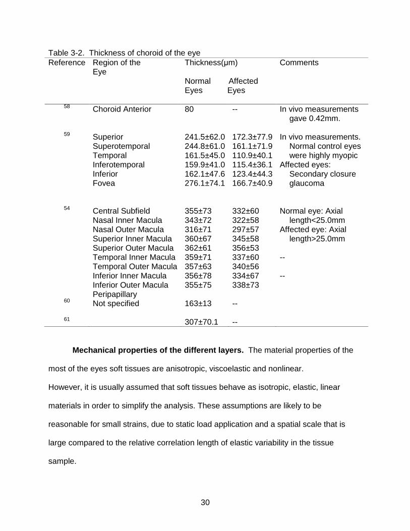
3-2 Thickness of choroid of the eye .......................................................................... 30

3-3 Thickness of retinal nerve fiber layer and retina as reported in literature ........... 31

3-4 Elastic properties of the different layers of the eye. ............................................ 32

3-5 Test case comparison of stress values of ADINA and analytical solution for a plate with a whole ............................................................................................... 40

3-6 Actual model comparison of stress values of ADINA and analytical solution ..... 42

4-1 Fixed parameters to study effect of diameter ..................................................... 44

4-2 Fixed parameters to study effect of retinal thickness .......................................... 52

4-3 Fixed parameters to study effect of material properties ...................................... 55

4-4 Conditions of IOP and BP. .................................................................................. 58

8

LIST OF FIGURES

Figure page 2-1 Formation and flow of the fluid in the eye ........................................................... 18

2-2 The system for outflow of aqueous humor from the eyeball into the conjunctival veins ............................................................................................... 19

2-3 Retinal layers. Low power micrograph of human retina ...................................... 20

2-4 Nerve fiber fascicles fan out as they overlie a medium sized blood vessel ........ 22

3-1 Plane stress model schematic used to analyze the retinal nerve fiber layer. ...... 34

3-2 OCT of a mouse eye. Arrows pointing at the retinal vessels .............................. 35

3-3 Variation of IOP and BP with time. ..................................................................... 36

3-4 Representation of a 2D plane stress element in ADINA ..................................... 37

3-5 Actual finite element model mesh from ADINA ................................................... 38

3-6 Test case schematic. .......................................................................................... 39

3-7 Superimposing plate with hole subject to tension and a thick cylinder pressurized from inside. ..................................................................................... 41

4-1 Representation of the radial lines where results were evaluated ........................ 45

4-2 Von-Mises stress distribution for all time steps for vessel diameter=100 and WLR=0.4 along radial 1,2,3 and 7. ..................................................................... 46

4-3 Normalized variation of stress along radial1 for different diameters A) Maximum stress B) Minimum stress. .................................................................. 46

4-4 The retinal mesh with effective stress field for the model for two load combinations. ..................................................................................................... 47

4-5 Maximum stress value across different radials(1,2,3 and 7) for different diameters. ........................................................................................................... 47

4-6 Pattern of strain yy for diameter=100 along radial 1,2,3 and 7, with WLR=0.4. .. 49

4-7 Normalized variation of strain yy along radial 2 for all diameters ........................ 49

4-8 Comparison of Maximum and minimum strain yy values in different radials for same diameter. ................................................................................................... 50

9

4-9 The pattern for strain zz for Radial1, 2, 3 and 7 for diameter =100 and WLR =0.4. ................................................................................................................... 50

4-10 The variation strain zz along different radials(1,2,3,7) for all diameter .............. 51

4-11 Normalized variation of strain zz for radial 1 for all diameters. ........................... 51

4-12 Normalized variation of stress along radial 3 for different retinal thickness. ....... 53

4-13 The variation of stress along different radials around the artery for different retinal thicknesses .............................................................................................. 53

4-14 Normalized variation of strain yy along radial 3 for different thicknesses. .......... 54

4-15 Variation of strain yy along different radials around the artery for fixed thicknesses ......................................................................................................... 54

4-16 Normalized variation of stress for different retinal moduli at radial 2. ................. 56

4-17 The variation of stress for each radial and for different retinal moduli ................ 56

4-18 Normalized variation of strain yy for different retinal moduli at radial 2. .............. 57

4-19 Variation in strain zz for each radial and different retinal moduli ........................ 57

5-1 Estimation of the area of nerve fibers exposed to higher stresses. .................... 61

10

LIST OF ABBREVIATIONS

ACG Angle Closure Glaucoma

BP Blood Pressure

FSI Fluid Structure Interaction

GON Glaucomatous Optic Neuropathy

IOP Intraocular Pressure

LC Lamina Cribrosa

OAG Open Angle Glaucoma

OBF Ocular Blood Flow

OCT Optical Coherence Tomography

ONH Optic Nerve Head

RNFL Retinal Nerve Fiber Layer

RPE Retinal Pigment Epithelium

11

Abstract of Thesis Presented to the Graduate School of the University of Florida in Partial Fulfillment of the Requirements for the Degree of Master of Science

FINITE ELEMENT STUDY OF NERVE FIBERS AROUND RETINAL ARTERIES AND

POSSIBLE RISK FACTORS FOR GLAUCOMA

By

Devesh Chugh

December 2012

Chair: Roger Tran-Son-Tay Major: Mechanical Engineering

Glaucoma is an irreversible optic neuropathy that causes loss of peripheral and

ultimately central vision. It is a pathologic condition in which there is a progressive loss

of retinal ganglion cells, specific visual field deficit, and a characteristic excavative

atrophy of the optic nerve. There are many forms and different subsets of this disease,

but the exact cause and pathophysiology are still unknown. Intraocular pressure (IOP)

has been identified as the most important factor. However, alone IOP is not able to

explain the cause of the disease. Other parameters, like blood flow, diameter of the

retinal arteries, layer thickness and material properties of the tissues need to be studied.

Many clinical observations have reported a change in the physical structure of the

retinal arteries and different layers of the retina in glaucoma. But there has been no

study on the correlation between how various factors like retinal thickness, diameter of

the artery and the material properties impact the retinal ganglion cells. A finite element

eye model has been created using commercially available software and the factors

mentioned above were studied.

The simulations help characterize the stress-strain field around the retinal

arteries in the retinal layer. Within the literature reported values of the parameters

12

studied, the diameter of the retinal vessels and the material properties have significant

impact onto the stress-strain field. We can conclusively say that in the nerve fibers near

the retinal arteries there are extremely high stresses as compared to stresses produced

only by IOP.

13

CHAPTER 1 INTRODUCTION

Glaucoma

Glaucoma is an irreversible optic neuropathy that causes loss of peripheral and

ultimately central vision. It is a pathologic condition in which there is a progressive loss

of retinal ganglion cells, specific visual field deficit, and a characteristic excavative

atrophy of the optic nerve head. In practice it has proven useful to speak about

glaucoma patients if they present either with elevated Intraocular pressure (IOP),

glaucomatous optic neuropathy (GON) or both1. Whereas a number of indisputable risk

factors, including elevated IOP, have been described, the pathogenesis leading to

glaucomatous optic neuropathy remains poorly understood. For an eye with glaucoma,

the reduction in visual sensitivity is a result of the loss of retinal ganglion cells and that

retinal areas with greater losses of sensitivity have undergone greater glaucomatous

losses of ganglion cells2-4. Half of the people who suffer from the disease do not even

know it until the disease has reached advanced stages5.

There are some clinical measurable factors that are now being used to diagnose

glaucoma like the retinal nerve fiber layer (RNFL) thickness. Studies have shown the

overall RNFL thickness average to be the best diagnostic parameter for glaucoma6-9.

Other studies have shown the inferior10-12 or superior 13 quadrant of the eye's RNFL

thickness average to be the best, in agreement with clinical observation that

glaucomatous optic nerve damage seems to begin. Also, the diameter of the retinal

arteries of glaucoma patients has been observed to vary from normal subjects. Studies

have shown that the vessel diameters decreases significantly with increasing glaucoma

14

stage independently of the patients' age 14-18. These factors when combined, affect the

mechanical environment (stress and strain distribution) of the retinal nerve fibers.

Data available in literature shows how the nerve fibers, in different parts of the

human body, behave when subject to mechanical stresses and strains. For example in

the peripheral nerves while 5% strain does not affect conduction, further elongation

decreases amplitude approximately linearly with strain19. The pressure threshold at

which the blood perfusion in sciatic nerves starts to decrease in diabetic rats is 24.1 mm

Hg and that in the normal controls is 47.1 mm Hg 20. The blood perfusion of the sciatic

nerve started to decrease at a mean pressure of 30.5mmHg and reached a stable lower

level of 30% of pre-compression value at 102.8 mmHg21.

In all the theories of the glaucoma, the effect of IOP has been taken into account,

but the effect of the retinal arteries, thickness of retinal layer and the material properties

onto the stress strain field of the RNFL has not been explored.

Objective

The focus of this thesis was to develop a finite element model which can

characterize the stress and strain field in the retinal nerve fiber layer, specifically around

the retinal arteries. The retinal artery is embedded inside the retinal nerve fiber layer

and exerts pressure on the nerve fibers all around it. To add to this, there is the

intraocular pressure (IOP) that acts on the inner limiting membrane of the retina.

This study includes the variation of factors like IOP, arterial blood pressure,

diameter of the retinal arteries, thickness of the retina and the material properties. Since

glaucoma involves the loss of retinal ganglion cells, we need to study the mechanical

environment in the retinal nerve fiber layer. The objective of this study is to characterize

the stress and strain distribution around the retinal nerve fiber layer and how some of

15

the clinical measurable parameters and material properties affect it. The variation of the

input parameters thickness, diameter, material properties and the loading conditions will

help us to establish in which area of the eye the retinal nerve fibers are exposed to

higher stress and strain values. This information can potentially help us to identify the

risk for loss of ganglion cells within the retinal nerve fiber layer.

Specific Aim

To develop 2D Finite Element Model for a cross-section of retinal nerve fiber

layer around the retinal arteries under different pressure loading conditions. We include

the three load bearing layers i.e. retina, choroid and sclera, in the posterior portion of

the eye. The arterial wall is embedded in the retinal layer and will be modeled as

separate within the retinal layer.

The material properties considered in this model are purely elastic properties.

Each layer will have different material properties. We will cover the physiological range

and use values as reported in the literature. Three values are used, two extreme values

and one in the middle. The range for different layers is:

Retina: Young's Modulus from 0.03MPa to 0.12MPa

Choroid: Young's Modulus from 0.15MPa to 0.25MPa

Sclera: Young's Modulus from 0.5MPa to 4.0MPa

Arterial Wall: Young's Modulus from 0.2MPa to 0.5MPa

The geometrical properties i.e. the diameter of the retinal artery, the thickness of

each layer varies in different regions of the eye. We are concentrating on the

physiological range. The values that will be used are 250 to 320μm for retinal layer, 280

to 370 μm for choroid, 900 to 1000 μm for sclera and 80 to 120 μm for the diameter. For

all the range reported above we use two extreme values and one middle value.

16

The pressure conditions inside the retinal artery (BP) and pressure inside the eye

(IOP) are also incorporated with suitable pressure functions. They are varied to capture

the different combinations of IOP and BP for the circadian variation in IOP and BP. The

range for IOP is 13mm Hg to 23 mm Hg and the range for BP is 80mm Hg to 120 mm

Hg.

The model will be solved using commercially available software ADINA (ADINA

R&D Inc., MA). The output from the model is the stress and strain fields around the

retinal artery. The von-mises stresses will be used to characterize the stress field and

the strains will be analyzed in two directions to characterize the stretch and

compression of the nerve fibers.

17

CHAPTER 2 BACKGROUND AND SIGNIFICANCE

Anatomy and Physiology of the Eye

Structure

The eye is a very complex organ that sends a huge amount of information to the

brain. It has a very specific design to capture and analyze light. The most important

parts of the structure, relevant to this thesis, are discussed in this section.

The outer shape of the eye is a non-symmetric sphere, flattened at the top and

the bottom part and an outside bulge at the front part. The outer shell is called the

sclera, which is visible to us as the white part. Sclera is the site of attachment of the eye

to external structures (muscles and connective tissues) and has portals for the passage

of blood vessels and nerves in and out of the eye22. It is light-tight so that light can only

enter through a small opening, called the cornea at the front, which is also the primary

refractive element of the eye. The cornea and sclera limbus are thin elastic sheets and

are made primarily of type I collagen fibrils 22, 23. The image of the object is formed at

the retina which is at the back of the eye, and the light is focused by the cornea, lens,

aqueous and vitreous humor. The lens contributes about one-third of the eye's total

dioptric power.

The Fluid System of the Eye

The fluid system (Figure 2-1) that we discuss here is responsible for all the

pressure that is exerted onto the retina, choroid and the sclera. To maintain the shape

of the eye formed by sclera and cornea it is necessary to provide pressure from the

inside of the eye, therefore the eye is filled with intraocular fluid. It maintains sufficient

pressure in the eyeball to keep it distended. This fluid in front of the lens is called the

18

aqueous humor and vitreous humor is between the posterior surface of the lens and the

retina. Total ocular volume is about 6.5ml of which 10% is aqueous humor. The

aqueous humor is a freely flowing fluid, whereas the vitreous humor, sometimes called

the vitreous body, is a gelatinous mass held together by a fine fibrillar network

composed primarily of greatly elongated proteoglycan molecules.

Eighty percent of the interior volume of the eye is vitreous and the longest optical

path from the cornea to the retina is through the vitreous22. Aqueous humor is

continually being formed in the ciliary processes at a rate of 2 to 3 microliters per

minute24, 25. The balance between formation and reabsorption of aqueous humor

regulates the total volume and pressure of the intraocular fluid.

Figure 2-1. Formation and flow of the fluid in the eye. Reprinted by permission from Elsevier Publications. Guyton & Hall: Textbook of medical Physiology, 11th Edition (Figure 49-19, Page 623) Elsevier, .All copyrights with Elsevier Publications, Philadelphia

The aqueous humor flows anterior to the lens and into the angle between the

cornea and the iris, then through a meshwork of trabeculae, finally entering the canal of

19

Sclemm, which empties into extraocular veins (as shown in Figure 2-2). The average

normal intraocular pressure is about 15 mm Hg, with a range of 12 to 20 mm Hg24.

The Retina

The light is focused on to the retina and retina transforms the light energy into a

signal to be communicated to the brain. The photoreceptors in the retina act as a group

they transform the pattern of light and shade in the retinal image into a corresponding

pattern of gradations in neural activity. The Figure 2-3 shows a typical histological

section of the retina and a representation of different cells along the thickness.

After the light passes through the lens system of the eye and then through the

vitreous humor, it enters the retina from the inside, that is it first passes through the

ganglion cells, then through the plexiform and nuclear layers before it finally reaches the

layer of rods and cones located all the way on the outer edge of the retina. This

distance is a thickness of several hundred micrometer, which varies from one part of the

eye to the other part of the eye24.

Figure 2-2. The system for outflow of aqueous humor from the eyeball into the conjunctival veins. Reprinted by permission from Elsevier Publications. Guyton & Hall: Textbook of medical Physiology, 11th Edition (Figure 49-21, Page 624) Elsevier, .All copyrights with Elsevier Publications, Philadelphia

20

The layer beneath the retina is called the choroid. The choroid serves a double

purpose: nourishment and absorption. The choroid carries blood to the retina and the

humors, providing nourishment to the eye24.

Optic Nerve Head (ONH)

All ganglion cell axons and all branches of the central retinal artery and vein

converge at the optic nerve head. Ganglion cell axons run in stereotypical pattern from

their bodies to the ONH, which is their site of exit from the eye. The optic disc is a weak

spot in the fundus of the eye because it is not reinforced by the sclera. It lacks

photoreceptors and is therefore called the blind spot of the eye. In glaucoma there is

characteristic atrophy of the optic nerve head and clinically optic disk damage is used to

monitor the progress of glaucoma.

Figure 2-3. Retinal layers. (Low power micrograph of human retina(wax histology): arrows, retinal vessels. Original magnification: x150. 26). Reprinted by permission from Elsevier publications. The Eye: Basic Sciences in Practice by John V Forrester, 2002, Chapter 1, Figure 1.23, Page 37. All copyrights with Elsevier, Philadelphia.

21

The nerve head can be divided into three structurally different parts: the laminar

portion, which is defined by scleral fibers that intersect the axons as they exit the eye

(lamina cribrosa), the prelaminar portion lying between the lamina and vitreous; and the

postlaminar portion, which is the first section of the optic nerve22. The lamina cribrosa is

considered as the primary damage site in the optic nerve head27, 28.

Blood Flow in the Eye

The blood supply to the eye arises primarily from the ophthalmic artery, which is

the first branch of the internal carotid artery. At various points from the ophthalmic

artery, different branches supply the eye and its associated structures. The central

retinal artery branches off to penetrate the optic nerve approximately 10 to 15 mm

behind the globe29.

Vasculature of the retina. Retina has two separate sources of blood supply,

one from the central retinal arteries and the other from the bottom layered choroid. The

retinal arteries and veins lie within the nerve fiber layer of the superficial retina26, 29. The

nerve fibers are observed to splay around the retinal arteries inside the retina. Figure 2-

4 shows a nerve fiber fascicles fan out as they overlie a medium sized blood vessel.

Mechanism of Glaucoma

The pathogenesis leading to glaucoma is still not clearly understood. The primary

causes of glaucomatous optic neuropathy are unknown. The disorder affects the

individual axons of the optic nerve, which may die by apoptosis. Scientists have

proposed two main theories, the Mechanical Theory and the Vascular Theory but none

has been able to clearly define the path and cause of the disease. The research is

proceeding in many different fronts: genetic, biochemical, cellular biological and

22

mechanical to name a few30. In this study we are concentrating on the mechanical

factors that may affect the ganglion cells and its axons.

Figure 2-4. Nerve fiber fascicles fan out as they overlie a medium sized blood vessel (appearing as a black void) in the equatorial region of a cat retina. Magnification X30031. Reprinted by permission ARVO from Zhang X, Mitchell C, Wen R, Laties AM. Nerve fiber layer splaying at vascular crossings. Figure 3. IOVS, July 2002, Vol. 43, No. 7, Page 2064. All copyrights with ARVO.

Mechanical theory1. An increased intraocular pressure (IOP) leads to

elongation, stretching and collapse of the laminar beams and their posterial

displacement (bowing). The axons of the retinal ganglion cells become damaged either

directly, by increased pressure and pressure gradient, or indirectly, by tissue

deformation. The axoplasmatic transport is impeded which may ultimately induce cell

death, for example due to a lack of trophic factors1.

Vascular theory1. The vascular theory of glaucoma considers glaucoma as a

consequence of insufficient blood supply due to either an increased IOP or other risk

23

factors reducing ocular blood flow (OBF). The main cause of this theory is the existence

of glaucoma in patients with low IOP (called normal tension glaucoma).

Prevalence and Types of Glaucoma

In open angle glaucoma the angle between the cornea and the iris is open and

while in angle closure glaucoma this angle is closed. Further, in some open glaucoma

patients high IOP is observed which is called high tension glaucoma and in some

patients low IOP is observed which is normal tension glaucoma (NTG). There were 60.5

million people with open angle glaucoma (OAG) and acute angle glaucoma (ACG) in

2010, which will increase to 79.6 million by 2020, and of these, 74% will have OAG.

Women comprise 55% of OAG, 70% of ACG, and 59% of all glaucoma in 2010. Asians

will represent 47% of those with glaucoma and 87% of those with ACG. Bilateral

blindness will be present in 4.5 million people with OAG and 3.9 million people with

ACG in 2010, rising to 5.9 and 5.3 million people in 2020, respectively 32.

In 2010 more than 2 million individuals in the United States were affected by

open-angle glaucoma. Owing to the rapid aging of the US population, the total number

of treatable OAG patients will increase to more than 3 million by 202032 and to 7.32

million by 205033. Studies consistently find that about half of those with glaucoma are

unaware they have the disease5.

Given an estimated prevalence of glaucoma in the United States of 2.2 million

people, this would represent a payer burden (largely Medicare and Medicaid) in excess

of $300 million/year over and above the cost of providing routine care for glaucoma,

such as intraocular pressure lowering medications and visual field testing 34.

24

Present Analytical and Numerical Modeling for Glaucoma

The eye and its tissues are not easily accessible, therefore modeling is the most

logical way to analyze the behavior of the tissue of eye and how they react to the

different parameters of the environment they are in.

A simple model35 uses the Laplace model to predict the stress onto the lamina

cribrosa, whereas there are others where ocular rigidity is defined to estimate the

stresses36. There are many other mathematical models 27, 37, 38, but the problem with

these models is that the assumptions used make the model are oversimplified. These

models do not depict the individual tissue behaviors and also they cannot individually

vary the physiological parameters that the eye and its tissues are subject to. Therefore,

these models cannot quantify the effects and the cause of glaucoma, which needs the

understanding of the individual tissues that are subject to variable parameters.

A numerical approach can incorporate more realistic conditions than analytical

models can and has been widely used in engineering to determine the mechanical

response of complex biological tissues. Previous numerical modeling has focused on

modeling the optic nerve head (ONH) and more specifically the lamina cribrosa (LC)

which is considered as the primary site of the damage within the optic nerve head.

Finite element models are made using the geometric and material property values from

experimental data as listed in the literature and with 3D reconstruction of the eye28, 39-49.

These models studied the effects of the size and eccentricity of the scleral canal

on the mechanical response of the ONH. They found that IOP-related stresses within

the connective tissues of the ONH could be substantial 41, 48. Eye specific models were

reconstructed by using images of histological sections from donor tissues of the human

eyes obtained from the eye bank 40, 49. These models were then used to study the

25

relative influences of geometry and material properties of the ONH to changes in IOP 40,

41, 45. In the study by Segal et al. parameterized study of various geometric and material

details of the ocular model to assess their impact on a host of outcome measures

identified the five most important determinants of ONH biomechanics as: the modulus of

the sclera, the globe radius of the eye, intraocular pressure, the modulus of the LC, and

the thickness of the sclera 42.

Basis of these models. The hypothesis that Segal et al. have adopted is they

want to cater to all types of glaucoma, as glaucoma occurs in eyes with high IOP and

low IOP and therefore the hypothesis that even at normal levels of IOP, the connective

tissues of the ONH are constantly exposed to substantial levels of IOP related stress.

The level of stress generated by normal levels of IOP is assumed to play a central role

in the physiology and, in some eyes, the pathophysiology of all three ONH tissue types.

Therefore these models study the ONH tissue to analyze its behavior under IOP to

ascertain the cause of glaucoma or what initiates the start of glaucoma. These models

do not look into the impact of the IOP and the retinal arteries on to the retinal nerve fiber

layer.

Significance

It is still not clear how the pathophysiology of glaucoma is initiated. The models

described above have given some insight about sclera and the ONH, but no study has

been performed to study the retinal layer from a mechanical point of view. Glaucoma is

essentially the loss of axons in the retinal nerve fiber layer and there are many

mechanical factors that cause the stresses and strains on the axons in this layer.

Studies have shown the overall RNFL thickness average to be the best diagnostic

parameter 6-8 for glaucoma. Other studies have shown the inferior10-12 or superior 13

26

quadrant RNFL thickness average to be the best, in agreement with clinical observation

that glaucomatous optic nerve damage seems to begin. However, its impact on the

ganglion cells and its axons in the retinal artery has not been studied. Since the retina is

essentially a plane with substantial area over which the blood vessels ramify, most

retinal pathology is local in its early stages and cannot easily affect the entire area. The

loss of the retinal ganglion cells can further affect the material properties of a substantial

area of retina.

Also, predominantly only IOP is attributed as damaging the axons in the nerve

fibers, the stresses by the arteries and blood pressure are not considered. In this study

we characterize these stresses in the RNFL that are caused by the retinal arteries. The

retinal blood vessels serve for nutrition of the retinal ganglion cells and their axons. The

size of the artery plays a significant role as it is embedded inside the retinal nerve fiber

layer and narrowing of retinal arterial calibers in subjects with glaucoma has been

demonstrated14, 15, 50.

Through the modeling of various tissues and arteries inside the retinal never fiber

layer and simulating realistic eye conditions, like varying the IOP and blood pressure

over time, we can gain an insight of how mechanical stresses affects the retinal nerve

fiber layer. Such a model could serve as a potential tool to help us to identify the risk for

loss of ganglion cells within the retinal nerve fiber layer.

27

CHAPTER 3 MATERIALS AND METHODS

Finite Element Model for the Retinal Nerve Fiber Layer

The eye is one of the most complex organs of the human body. The conditions

inside the eye vary from one point to the other. Therefore, to analyze the retinal nerve

fiber layer from a mechanical point of view we need to make simplifying assumptions

and consider the most important parameters. We can point out the following parameters

that can affect the nerve fibers around the retinal arteries.

Geometrical factors. The geometrical factors go into defining the physical

parameters of the environment in our model. These are listed as follows.

Diameter of the retinal artery

Radius of the eye (Curvature/change of direction of flow)

Length of the artery

Thickness of the different layers of the eye: Retina, Choroid, Sclera, Artery Wall

Branching of the arteries

Mechanical properties of different layers. The material properties define how

material behaves to the applied load. These are listed as follows

Retina

Choroid

Sclera

Artery wall

Flow properties. The flow properties determine the pressures and are listed as

follows.

Pressure outside the artery(IOP)

Pressure inside the artery(arterial pressure)

Viscosity of the blood

Blood flow rate

Diameter of the retinal artery. The retinal arterial diameters which have a

major influence on the arterial blood pressure, owing to Hagen–Poiseuille’s law and are

28

therefore of major clinical interest. The retinal artery diameter varies from the point of

bifurcation to the very end of these arteries. The vasculature of each and every human

being is different and there are some mean values for the retinal diameters that are

based upon population surveys. These population-based data suggest that generalized

retinal arteriolar narrowing, an indicator of localized vascular change, is significantly

associated with optic nerve damage caused by OAG17.There is variation in the value

reported in literature for a specific region of the eye. Diameters from some of the major

population studies and some experimental studies are listed in Table 3-1.

Table 3-1. The values of the retinal artery diameter as reported in literature.

Reference Region of the Eye

Diameter(μm) Normal GON Eye Eye

Comments

14 Superotemporal 106±18 89±17 For Age <65: Caliber measured 105±18 88.8±16 For Age >65 Inferortemporal 113±20 88.6±14 For Age <65: Caliber measured 107±14 92.4±18 For Age >65

17 Not Specified 183±2.6 194±0.4 Measurements 0.5 to 1.0 disk

diameter from ONH. They used a formula given in 51, this formula gives higher values and was later corrected in 52

18 Superotemporal 115±18 87.3±18 Measurements just outside the

margin of optic disk. Visupac software used.

Inferotemporal 110±16 87±21 Superonasal 96±14 72±17 Inferonasal 89±16 71±18 16 Superotemporal 111±16 112±16 Measurement at optic disk border.

Caliber measured. Measurement of the temporal

superior and inferior vessels

53

Inferotemporal Superornasal Inferotemporal Not specified

117±17 97±15 94±14

101±15

117±86 95±12 91±12

100±8

29

Radius of the eye globe. The eye is not exactly spherical in shape. The end to

end distance varies from one point to other. It is maximum from anterior to the posterior

section and minimum from the top to bottom section. The anterior to posterior distance

is higher because of the bulge out of the cornea, the distance is usually between 22mm

to 23.5mm22. Since the retina is essentially a plane with substantial area over which the

blood vessels ramify, we can ignore the effect of the blood vessel curvature.

Thickness of the different layers of the eye. The properties of the different

layers of the eye are not spatially uniform and they vary from point to point. This applies

to all the layers of the eye. This impacts the load distribution in the nerve fiber layer and

the blood arteries. The thicknesses of the different layers involved in this analysis are

tabulated in Table 3-2.

The difference in thickness also arises in these values because different

approaches/algorithms are used to analyze the image data. For example in some

studies 54 retinal thickness is defined from internal limiting membrane and retinal

pigment epithelium, and in a different study 55 it is defined as between the vitreoretinal

interface and the inner and outer segments of the photoreceptors. Table 3-2 and 3-3 list

all the reported values of thickness of the choroid and the retina respectively.

The sclera is thickest at the posterior pole (996±181 μm), thinnest at the equator

(491±91 μm) and the thickness is in between at the corneoscleral limbus (588±63

μm)56. Similar results were reported in another study where the range of thickness was

reported between 1000 μm to 900 μm near the optic nerve to 250 μm at the equator and

390 μm at limbus57. There has been more convergence on the thickness of sclera as

compared to other layers because of its high rigidity.

30

Table 3-2. Thickness of choroid of the eye

Mechanical properties of the different layers. The material properties of the

most of the eyes soft tissues are anisotropic, viscoelastic and nonlinear.

However, it is usually assumed that soft tissues behave as isotropic, elastic, linear

materials in order to simplify the analysis. These assumptions are likely to be

reasonable for small strains, due to static load application and a spatial scale that is

large compared to the relative correlation length of elastic variability in the tissue

sample.

Reference Region of the Eye

Thickness(μm) Normal Affected Eyes Eyes

Comments

58 Choroid Anterior 80 -- In vivo measurements gave 0.42mm.

59 Superior 241.5±62.0 172.3±77.9 In vivo measurements.

Normal control eyes were highly myopic

Affected eyes: Secondary closure glaucoma

Superotemporal Temporal Inferotemporal Inferior Fovea

244.8±61.0 161.5±45.0 159.9±41.0 162.1±47.6 276.1±74.1

161.1±71.9 110.9±40.1 115.4±36.1 123.4±44.3 166.7±40.9

54

60

61

Central Subfield Nasal Inner Macula Nasal Outer Macula Superior Inner Macula Superior Outer Macula Temporal Inner Macula Temporal Outer Macula Inferior Inner Macula Inferior Outer Macula Peripapillary Not specified

355±73 343±72 316±71 360±67 362±61 359±71 357±63 356±78 355±75 163±13 307±70.1

332±60 322±58 297±57 345±58 356±53 337±60 340±56 334±67 338±73 -- --

Normal eye: Axial

length<25.0mm Affected eye: Axial

length>25.0mm -- --

31

Table 3-3. Thickness of retinal nerve fiber layer and retina as reported in literature

Reference Region of the Eye

Thickness(μm) Normal Affected Eyes Eyes

Comments

62

Temporal quadrant Superior quadrant Nasal quadrant Inferior quadrant

170±58 240±57 220±70 266±64

-- -- -- --

RNFL defined from inner limiting membrane to Bruch's Membrane

63 Temporal Superior Nasal Inferior

89.9±15.6 134.6±23.3 91.9±28.9 138.1±23.2

49.4±23.9 77.9±31.2 53.0±36.0 76.3±31.2

Affected eye: Advanced glaucoma

64 Perifoveal avg. 211.4±16.8 185.7±16.8

55 Center Fovea Mean Fovea Temporal Inner Macula Superior Inner Macula Nasal Inner Macula Inferior Inner Macula Temporal Outer Macula Superior Outer Macula Nasal Outer Macula Inferior Outer Macula

157.8±3.2 191.6±2.7 255.6±1.9 272.2±2.1 269.3±2.0 266.8±2.0 221.0±1.8 240.7±2.1 257.6±2.2 230.3±1.9

-- -- -- -- -- -- -- -- -- --

Retina defined as

between vitreoretinal interface to inner and outer segments of photoreceptors

54 Central Subfield Nasal Inner Macula Nasal Outer Macula Superior Inner Macula Superior Outer Macula Temporal Inner Macula Temporal Outer Macula Inferior Inner Macula

256±13 321±14 297±20 315±15 281±13 310±14 267±13 315±14

-- -- -- -- -- -- -- --

retinal thickness is defined from internal limiting membrane and retinal pigment epithelium

65 Superior Inferior Temporal Nasal Mean

146.6±32.2 143.5±32.9 66.9±34.6 117.2±33.1 119.7±28.1

-- -- -- -- --

Only Nerve fiber layer thickness

500 μm from the ONH

65 Superior Inferior Temporal Nasal Mean

133.5±34.7 128.7±42.0 91.5±35.8 89.2±31.0 110.7±30.9

-- -- -- -- --

Only Nerve fiber layer thickness

750 μm from the ONH

32

Table 3-3. Continued

Reference Region of the Eye

Thickness(μm) Normal Affected Eyes Eyes

Comments

65 Superior Inferior Temporal Nasal Mean

316.9±48.1 286.1±50.4 223.5±23.9 271.3±30.6 277.6±33.4

-- -- -- -- --

Retina: from vitreoretinal interface to RPE

500 μm from the ONH

65 Superior Inferior Temporal Nasal Mean

285.0±32.7 269.2±35.2 253.5±36.3 239.0±30.6 262.2±30.3

-- -- -- -- --

Retina: from vitreoretinal interface to RPE

750 μm from the ONH

Table 3-4. Elastic properties of the different layers of the eye.

Reference Layer (Region)

Elastic modulus (E) kPa

Model Comment

66 Retina 20 Bovine Invitro experiment and mathematical model

67 Retina 1.0 to 2.09 Porcine Spatial mapping of E. E defined at steps from ONH

68 Retina 100 to 110 Porcine Different strain rates used. 69 Retina 19.5±12.2 to

107.8±58 Porcine Tension test

70 Retina-Choroid Combined

15.63±4.25 Human In-vivo measurements

58 Choroid Anterior Posterior

2.2±1.5x102 7.5±7x102

Human In vitro testing. Tension test.

69 Choroid 1842±1221 to 3739±2638

Porcine Tension test in different environmental conditions.

71 Peripappillary Sclera

2930 to 6150 Human Tension test in different environmental conditions.

72 Sclera 1.1±0.8 to 1.47±0.33

3.87±.57 to 4.36±0.60

Human Porcine

Drained Secant Modulus for both cases.

73 58

Sclera Sclera

33.378 200 to 2600

Human Human

Average of several values Posterior Sclera

74 Sclera 4940±1220 to 7146±1580

Monkey

33

Again as for the thickness, the material properties of the sclera are mostly

studied and well documented in the literature. Other layers like the choroid, retina have

had very little focus from this point of view, but recently there have been few studies to

determine the material properties of the other layers. There is no convergence in the

reported values when compared to other studies66-70, 74, 75. Table 3-4 lists the elastic

modulus for the different layers being studied in this study. There are few reported

studies on the viscoelastic properties of the sclera, and this has been limited to monkey

and rabbit models74, 75.

Finite Element Model in ADINA

We use a simplified model to analyze the effect of the various geometrical and

material properties that have been listed in the previous section. To focus on the how

the stress-strain field in nerve fiber layer is affected all around the retinal arteries, we

take a cross-section of the retinal artery and the different layers around it as shown in

the Figure 3-1.

Computational domain. The domain is shown in the Figure 3-1. There are

three different tissue layers, retina, choroid and sclera. The artery is embedded in the

retinal layer. Since the arteries are not fixed at the ends inside the eye, we can reduce

the problem to a 2D plane stress model. The nodes at the interface between different

layers are shared to ensure contact between the layers. For example, the artery is free

to expand and it deforms the retinal layer around it and therefore causes the stress and

strain in retinal layer. Similarly, the nodes between retina and choroid are shared and

nodes between choroid and sclera are shared. The retina is loaded from top with the

IOP and the artery has internal pressure acting on the inside surface. The outside

vertical edges, for all the three layers, are constrained to move only in Z direction

34

(edges L1 to L6 as shown in Figure 3-1). The width of the model is 700µm. The bottom

edge is fixed as this is the point where eye is attached to the body (edge L7 in the

Figure 3-1). The tissue layers retina, choroid, sclera and the artery wall layer are

attributed linear elastic material properties with different elastic modulus as reported in

the literature.

Figure 3-1. Plane stress model schematic used to analyze the retinal nerve fiber layer.

Assumptions in this Model

Isotropic-elastic material properties for each layer. The reason for this was there were no visco-elastic properties reported in the literature for retina and choroid.

Plane stress model. Since the arteries are not fixed in the retinal layer, a plane stress assumption is assumed.

Retinal artery in the model is geometrically centered in the retinal layer.

35

We assume this cross-section of the retina is near the optic nerve head and far away from the retina edge (i.e. within the white circular border area as shown in Figure 3-2 left image, the radius of the circle being 5 times the radius of optic disk). The reason for this is that we want to analyze the effect of large arteries, the artery diameter is highest near the optic nerve head and it decreases as we move away from optic nerve head.

Figure 3-2. OCT of a mouse eye. Arrows pointing at the retinal vessels. A) Front view

of the mouse eye in OCT. B) A cross-section, showing the artery and different layers of the eye.

No thermal effects, temperature does not affect the output i.e. stress and strain.

The shear traction by the vitreous humor onto top layer of the retina is negligible and not accounted in the study. Viscous effects between different layers are also neglected. We have also neglected the shear gradient by the blood flow on the walls of the retinal vessels.

No fluid flux due to pressure gradient across tissues.

Boundary Conditions

Degrees of freedom x-translation, y-rotation, x-rotation and z-rotation are constrained. Only free degrees of freedom are y-translation, z-translation. These follow from plane stress condition.

The effect of the retinal arteries is negligible after a distance of ~300μm from the artery. This leads us to a width of L4 ~700 μm to analyze the effect of one retinal artery.

Retina Edge

X Y

Y

Z

Cross-section of the retina with artery

Cross-section of the retina with artery

A B

X

C’

C

36

IOP is applied to the top edge. The vertical edges (L1-L6 in Figure 3-1) are constrained to move only in the vertical (Z) direction. Figure 3-2 which shows an OCT of an eye of a mouse. In the image on the left, we can see the artery and vein network and in the right image we can see a cross-section (C-C’) at one location. The vertical edges of the model will have negligible expansion in the Y direction (see Figure 3-2). The lateral expansion will only be pronounced near the retina edge in outward direction(X direction) away from optic nerve head of the retina. If we observe in vertical cross-section of the OCT (right image of Figure 3-2), its vertical edge (pointed with arrow) will be forced from both side (in Y direction) of the material and hence expansion in Y direction inside the circular region will be minimal. Hence the boundary condition of vertical edges to move in vertical direction (Z direction) can be applied. Since it is a plane stress model, we do have non zero strain in X direction.

The bottom edge (L7 in Figure 3-1) is the outer layer of the sclera, where sclera is connected to the rest of the body and therefore constrained to not to move in all directions.

The top layer is exposed to IOP, a pressure function is used to include the variation of the IOP (refer Figure 3-3)

Arterial inner surface of the blood vessel is subject to the blood pressure. Another pressure function is used to describe to capture this variation.

Figure 3-3. Variation of IOP and BP with time. (Please note: this is not a time dependent problem, IOP and BP are varied to capture different load combinations that occur within the eye due to circadian rhythms. In ADINA, for soft tissues, due to convergence issues we cannot jump from one load to other load in one step, we need to go in small load steps)

37

Figure 3-4. Representation of a 2D plane stress element in ADINA (ADINA Inc., MA)

Details about the model in ADINA. A plane stress element in ADINA is as

shown in the Figure 3-4. Equation 3-1 represents the equation which is solved and for

the calculation of all element matrices and vectors, numerical Gauss integration is used.

In linear analysis using ADINA, the finite element system equilibrium equations to

be solved are

(3-1)

Where K is the stiffness matrix, U is the displacement vector and R is the load

vector. The two material constants used to define the constitutive relation are =

Young's modulus, = Poisson's ratio.

Mesh size and sensitivity. Two dimensional nine node elements were used

throughout the model. The mesh sensitivity was checked in the preliminary stages with

three different mesh sizes. The number of elements varied in the three cases were

4879, 10943, 43467. For example, for a retinal thickness of 280, choroidal thickness of

330, sclera thickness of 960 and retinal diameter of 100 the total number of elements

were 10943. Error for this specific case was then checked and found to be ~0.4% for

the retinal layer and ~1% for the arterial wall. For choroid and sclera it was O (~10-4).

With a mesh size of 5 units (total elements = 43647, for the same example mentioned

above) the results were within 0.5% with respect to mesh size of 10 and with mesh size

38

15 units (total elements = 4879, for the same example mentioned above) the difference

in results were within 2.2%. Mesh size of 10 was then used to do all the simulations.

Actual finite element model is shown in Figure 3-5.

Figure 3-5. Actual finite element model mesh from ADINA

Model Validation

Test Case. To check the ADINA modeling and solutions, we compared results

with a benchmark problem of an infinite plate with a hole in tension (Figure 3-6). There

39

is an analytical solution for the stress on the horizontal line of symmetry which is given

by Equation 3-276. This analytical solution is valid for linear elastic properties and for the

hole dimension being very small compared to the length of the plate. ADINA was then

used to solve same problem, to simulate infinite plate the width and height of the plate

were kept very large as compared to the hole dimension. The hole dimension was 5mm

and the tensile stress was 25MPa on the top edge of the plate. Results of analytical

solution (Equation 3-2) and ADINA are compared in Table 3-5.

(( (

)

) ( (

) )) (3-2)

Figure 3-6. Test case schematic.

40

The percentage error was acceptable considering the limitation that the

numerical model was not actually infinite. A second validation check was then

performed for the actual model.

Table 3-5. Test case comparison of stress values of ADINA and analytical solution for a plate with a whole

Distance from

center Ratio

Analytical Plate Stress

ADINA Stress

Percentage error

R(mm) A/R (MPa) (MPa) 5.00 1.000 75.000 74.709 -0.39

5.65 0.885 57.746 59.827 3.48

6.30 0.793 47.700 48.477 1.60

6.96 0.719 41.465 41.038 -1.04

7.61 0.657 37.391 37.357 -0.09

8.26 0.605 34.612 34.570 -0.12

8.91 0.561 32.647 32.209 -1.36

9.57 0.523 31.215 30.816 -1.30

10.22 0.489 30.144 29.774 -1.24

10.87 0.460 29.324 28.922 -1.39

11.52 0.434 28.684 28.365 -1.13

12.17 0.411 28.176 27.875 -1.08

12.83 0.390 27.766 27.482 -1.03

13.48 0.371 27.430 27.208 -0.82

14.13 0.354 27.153 26.962 -0.71

14.78 0.338 26.921 26.755 -0.62

15.43 0.324 26.725 26.622 -0.38

16.09 0.311 26.557 26.468 -0.34

16.74 0.299 26.414 26.328 -0.33

17.39 0.288 26.289 26.215 -0.28

18.04 0.277 26.181 26.111 -0.27

18.70 0.267 26.086 26.010 -0.29

19.35 0.258 26.002 25.929 -0.28

20.00 0.250 25.928 25.854 -0.28

Actual model validation. A second check was performed to validate the actual

model. By superimposing the stress fields (Figure 3-7) of an infinite plate with a hole

subject to tension and a very thick cylinder subject to internal pressure were used to

41

compare the results obtained from ADINA. Our particular problem does not match the

exact analytical solution of the problem mentioned as in our case the plate is finite and

the pressurized hole is being approximated as a very thick cylinder, therefore the

analytical results will give reasonable values only near the artery wall, the deviation will

increase as we move away from the artery wall.

Figure 3-7. Superimposing plate with hole subject to tension and a thick cylinder pressurized from inside.

Analytical solution for stress for a thick cylinder problem is given by Equation 3-

376

(3-3)76

K and C are constants and are determined based on boundary condition of the cylinder.

Since we are approximating the cylinder to be infinitely large, the boundary condition for

the cylinder analytical solution become

42

Where p is the blood pressure inside the artery ( ) and A being the internal

radius (45µm in this specific case). Using above boundary conditions Equation 3-4

reduces to

(3-4)

Analytical solution for the plate with σ =0.00227MPa and A=45µm were calculated using

Equation 3-3. This solution will only hold good for stress near the hole.

ADINA results from a model with exact conditions of pressure and hole dimension (with

artery radius=45µm, IOP=0.00227MPa and BP=0.01295MPa) were compared with the

resultant analytical stress. Sigma 1(in Table 3-6) is calculated from Equation 3-2 and

sigma 2 is the stress for cylinder which is given by Equation 3-4. The two stresses

sigma 1 and sigma 2 are then added and compared with ADINA stress. Comparison is

presented in Table 3-6.

Table 3-6. Actual model comparison of stress values of ADINA and analytical solution Distance

from hole

center

Relative distance

from hole

Approximate Plate Stress (Equation

3-2)

Approximate Hole Stress (Equation

3-4)

Total Stress

ADINA STRESS

Percentage error

R(mm) A/R sigma1 (MPa)

sigma2 (MPa)

(MPa) (MPa)

45.00 1.0000 0.00680 0.01295 0.01975 0.01979 0.2302 46.02 0.9778 0.00646 0.01238 0.01884 0.01886 0.1028 47.04 0.9566 0.00615 0.01185 0.01800 0.01792 -0.4302 48.06 0.9363 0.00587 0.01135 0.01722 0.01749 1.5045 49.08 0.9169 0.00562 0.01089 0.01651 0.01705 3.2044 50.10 0.8982 0.00539 0.01045 0.01584 0.01569 -0.9489 51.12 0.8803 0.00519 0.01003 0.01522 0.01538 1.0406 52.14 0.8631 0.00500 0.00965 0.01464 0.01507 2.8311

43

Percentage error in stress values very near the hole (for the A/R values less than

0.86), was always less than 3.3%. Since these are only approximate analytical solution

that we are comparing with, we can conclude that the results obtained from ADINA are

acceptable and hence same scheme of modeling was used throughout the study.

44

CHAPTER 4 RESULTS

Case 1: Effect of Variation of Diameter

Table 4-1. Fixed parameters to study effect of diameter

Layer Thickness Elastic modulus Poisson’s ratio

Retina 280 70kPa 0.49 Choroid 330 187kPa 0.49 Sclera 960 3000kpa 0.48 Vessel Wall WLR*=0.4 300kPa 0.4

Material properties: Linear Elastic properties, isotropic Varying parameter: Vessel Diameters: 80, 90, 100,110 and 120μm. *WLR= Wall to lumen ratio

Physiological relevance. The diameter would cover all the major regions of the

eye. WLR is average value. All the values used are in the tables which summarized the

geometric properties in Chapter 3. To better quantify the results, we have evaluated

stress and strain fields at different radial lines as shown in Figure 4-1.

Stress. Maximum stress is near the wall and then the stress decreases as we

go away from the wall. The pattern for variation of stress as we move away from the

artery wall is similar for all the diameters (80-120). To show specific patterns, we have

plotted data along different angular radials, this is as shown in Figure 4-2. As this is a

symmetric problem, other radial plots are omitted in this Figure. The pattern for radial 3

and 7 is a little different than for the others, because of the small length of the radial

over which the stress is observed. For other diameters, there is a change in the

magnitude of the maximum and minimum values for the stress. Figure 4-3 a and b

depict this pattern of variation of maximum and minimum stress. For normalization the

value corresponding to the lowest parameter i.e. 80µm diameter are used, this practice

is followed for all the normalized curves in this thesis. Contours of the stress distribution

for two load combinations is shown in Figure 4-4.

45

Figure 4-1. Representation of the radial lines where results were evaluated

With increase in the vessel diameter it is expected that the maximum stress will

increase for all the other parameters being fixed. For the variation of minimum stress,

which occurs at the away from the wall and is affected only by the IOP, the observed

pattern is because the dimensions of the retina are fixed and the same point is now

closer to the vessel wall (for higher diameter), therefore the minimum stress value

increases.

To depict the effect of variation of stress values for one diameter at different

radial position we have included Figure 4-5. The stress values peak for radials 3 and 7.

Similarly the minimum value varies across all the radials.

Strain yy. The strain yy(in the horizontal direction) changes nature as we move

around the artery wall.

46

Figure 4-2. Von-Mises stress distribution for all time steps for vessel diameter=100 and WLR=0.4 along radial 1,2,3 and 7. The pattern is same for all other diameters as well. However the magnitude of stress change for different diameters.

Figure 4-3. Normalized variation of stress along radial1 for different diameters A) Maximum stress B) Minimum stress. The variation of minimum and maximum value is same for all other radials as well. Base stress values correspond to the specific case of 80µm diameter.

A B

47

Figure 4-4. The retinal mesh with effective stress field for the model for two load combinations. For the above image the IOP=21.1 and BP=116.5 and for the bottom image the IOP=21.3 and BP=77.7(All pressures in mmHg). The case parameters are diameter=100, retinal thickness =280, E=0.07MPa(retina)

Figure 4-5. Maximum stress value across different radials(1,2,3 and 7) for different diameters.

48

But as have symmetry, the strain patterns are same for radials 1 and 5 and 2,4,6

and 8 and 3 and 7. The strain values along these radial pairs are very close. The

variation of the strain yy along radial 1, 2, 3 and 7 is as shown in Figure 4-6. Along

radial 1, the nerve fibers are compressed along this direction. The value is maximum

compressive near the wall and strain reduces as we move away. As observed for the

stress the value of the maximum compressive strain in yy direction is maximum near the

vessel wall and this value increases as the diameter increases. Figure 4-7a and b show

the minimum and maximum value pattern across different diameters. The pattern is

similar to the variation of the stress values along the same radial line. The minimum and

maximum stress and strain yy occur at the same positions as for the stresses. The

variation of maximum and minimum strain yy for all diameters along different radials is

shown in Figure 4-8.

Along radial 2 the nerve fibers are compressed. The value is maximum

compressive near the wall and strain reduces as we move away. The pattern of

variation of maximum and minimum values across radial 1, 3, 6 and 8 is same as for

radial 2, as shown in Figure 4-7. The minimum and maximum stress and strain yy occur

at the same positions as for the stresses.

Along radial 3 the big difference is that in this case the nerve fibers are stretched

and are in tension. The value is maximum tensile near the wall and strain reduces as

we move away. The pattern of variation of maximum and minimum values across others

radials is same as for radial 2, as shown in Figure 4-7.

Strain zz. As we clubbed the strains along yy direction, we observe similar

grouping for strain zz (Radial 1 and 5, radial 2, 4, 6 and 8, 3 and 7).

49

Figure 4-6. Pattern of strain yy for diameter=100 along radial 1, 2, 3 and 7, with WLR=0.4.

Figure 4-7. Normalized variation of strain yy along radial 2 for all diameters A) Minimum

strain yy B) Maximum strain yy. Base strain values correspond to specific case of 80µm diameter.

Along radial 1 and 2, the strain zz changes its nature as we move away from the

artery walls. Since radial 1 and 5 are along the horizontal axis, due to the expansion of

the artery the nerve fibers along these radials are in stretched condition, but as we

move away this effect reduces and due to IOP they get compressed.

A B

50

Figure 4-8. Comparison strain yy values in different radials for same diameter. A)

Minimum strain yy. B) Maximum strain yy

Figure 4-9. The pattern for strain zz for Radial1, 2, 3 and 7 for diameter =100 and WLR =0.4. (This strain is for the maximum strain zz configuration)

The distance from the vessel wall where this transition occurs increases with

increase in the diameter. Figure 4-9 show the pattern for radial1, 2, 3 and 7. The

variation of strain zz along different radials, for one diameter is as shown in Figure 4-10.

The variation of maximum and minimum values for radial 1 across all diameters is as

shown in Figure 4-11. Along radial 3 and 7 the nerve fibers remain in compression only.

A B

51

The nerve fibers above and below the artery are subject to constant compression from

the IOP and the expanding arteries.

Figure 4-10. The variation strain zz along different radials (1, 2, 3, 7) for all diameters A) Minimum strain zz B) Maximum strain zz

Figure 4-11. Normalized variation of strain zz for radial 1 for all diameters. A) Minimum

strain zz B) Maximum strain zz. Base strain values correspond to 80µm diameter case.

Case 2: Effect of Thickness of Retina

Among the three layers studied, the retinal thickness is observed to have some

impact on the stress distribution. Therefore, results for only the retinal thickness are

presented. Same model is used for this analysis. The summary of all the properties is

listed in Table 4-2.

A B

A B

52

Table 4-2. Fixed parameters to study effect of retinal thickness

Layer Thickness/Diameter Elastic modulus Poisson’s ratio

Retina -- 70kPa 0.49

Choroid 330 187kPa 0.49

Sclera 960 3000kPa 0.48

Vessel Wall Dia=90 , WLR*=0.4

300kPa 0.4

Material properties: Linear Elastic-isotropic properties only. Varying parameter: Retinal thickness: 250, 280 and 330 μm.

Physiological relevance. The retinal thickness would cover all the major

regions of the eye. WLR is average value. This is all referenced in the tables which

summarized the geometric properties in Chapter 3.

Stress. The stress variation pattern is same as in the case 1. Here we will

describe the variation in stress magnitude across the different thicknesses of retina.

As we increase the thickness of retina, stress decreases for most of the locations

around the artery, except radial 1 and 5 where the stress increases (by 0.1%) when we

first increase the thickness from 250 to 280(12%) and then it decreases (0.5%). Figure

4-12 shows the variation of maximum and minimum value of stress along radial 3.

Pattern for maximum stress in radials 1 to 8 is same and decreases continuously except

radial 1 and 5, for which there is slight increase in first thickness increase from .250 to

280. However, if we talk of percentages the change in stress values are most significant

along radial 3. There is almost 7% increase in the maximum stress value as we

decrease the thickness from 320 to 250 μm (21% decrease). For radial 7 its about 5%.

The variation of minimum and maximum along different radials around the artery for

fixed thicknesses is shown in Figure 4-13.

53

Figure 4-12. Normalized variation of stress along radial 3 for different retinal thickness. A) Minimum stress. B) Maximum stress. Base stress values are for specific case of Retina thickness 250µm

Figure 4-13. The variation of stress along different radials around the artery for different retinal thicknesses A) Minimum stress B) Maximum stress

Strain yy. Figure 4-14 shows the changes in the values of maximum and

minimum strain yy with different retinal thicknesses. The pattern of variation along a

particular radial is same as discussed in section 1 of this Chapter. The maximum value

of strain yy change at radial 2 is approximately 15% and minimum strain yy which

occurs far away from artery wall it is 40% as we decrease the thickness from 320 to 250

μm.

A B

A B

54

Figure 4-14. Normalized variation of strain yy along radial 3 for different thicknesses. A) Minimum strain yy B) Maximum strain yy. Base stress values are for specific case of Retina thickness 250µm

Figure 4-15. Variation of strain yy along different radials around the artery for fixed

thicknesses. A) Minimum strain yy B) Maximum strain yy

Strain zz. The pattern is same as shown in Figure 4-15 shows the changes in

the values of maximum and minimum strain yy with different retinal thicknesses, along

different radials. The pattern of variation along a particular radial is same as for the

different diameter (case 1) section of this Chapter. However, there is change in

magnitude of the value and these are depicted in the Figure 4-15. Again, the

A B

A B

55

percentage change in the maximum values is along radial 3 and 7 when we decrease

the thickness from 320 to 250.

Case 3: Effect of Material Properties of Different Layers.

With a standard geometry we varied the material properties of the different tissue

layers, to see the impact on stress and strain of the nerve fibers around the artery wall.

However the impact of the choroid and the sclera was very small and the variation in

stress was within 1% for different young’s modulus of choroid and sclera. However,

change in only the young’s modulus of retina did impact the stress values significantly

and therefore only the results of variation of retinal layer’s young’s modulus is

presented. Same model was used to study the impact.

Table 4-3. Fixed parameters to study effect of material properties

Layer Thickness/ Diameter Elastic modulus Poisson’s ratio

Retina 280 𝑚 -- 0.49

Choroid 330 𝑚 187kPa 0.49

Sclera 960 𝑚 3000kPa 0.48

Vessel Wall Dia=90 𝑚, WLR=0.4

300kPa 0.4

Stress. The pattern of variation of stress is same as in the case 1. However, the

change in stress values with reported elastic moduli is very high. The value of stress

increase to almost 60% as we increase the elastic moduli of retinal layer in the given

physiological range as reported in literature. Please note that we only varied the young’s

modulus of the retinal layer. If we increase young’s modulus of all the different layers

with same factor, we do not observe any change in the stress values, which should be

expected. But when we change only material property of one layer we observe change

in the stress values. The variation of the maximum and the minimum values of stress

are shown in Figure 4-16.

56

The variation of stresses along different radials for different moduli is shown in

Figure 4-17. Again, the gap between stress values for different elastic moduli is

significant.

Figure 4-16. Normalized variation of stress for different retinal moduli at radial 2. A) Maximum stress B) Minimum stress. Base values correspond to stress for moduli of 0.03MPa

Figure 4-17. The variation of stress for each radial and for different retinal moduli A) Maximum stress B) Minimum stress

Strain zz: The patterns for strain zz are very similar to the strain yy. To show

how the elastic moduli affects the strain zz in the nerve fiber, see the Figure 4-19.

A B

A B

57

Figure 4-18. Normalized variation of strain yy for different retinal moduli at radial 2. A) Minimum strain yy. B) Maximum strain yy. Base values correspond to the case of E=0.03MPa.

Figure 4-19. Variation in strain zz for each radial and different retinal moduli. A) Minimum strain zz B) Maxuimum strain zz

Effect of BP and sensitivity to IOP. The pressure conditions in the eye keep

varying with time. To study the impact of change in stress values with different IOP

conditions, we calculated the percentage change in the stress with given IOP conditions

and varying BP. The various IOP and BP conditions are listed in Table 4-3. Basically

this helps to understand the variation in RNFL stresses in the eye of patients with

different IOP conditions (high tension and low tension glaucoma). The variation for the

first set of IOP condition(Average to high IOP) was approximately equal for all the

A B

A B

58

thicknesses ~ 22.4%, 11.4% and 4.7% for a jump from minimum to average BP,

average to high BP and finally from high to maximum BP(49% increase). These

variations were within ± 1 % for all the different radials. For high and low IOP the

variation from minimum BP to average BP (25% increase) and from average to

maximum(19% increase) was ~23% and ~15% which is similar to the previous case.

Since we have linear elastic properties, we do not observe any significant effect of BP

on RNFL stress with the changing IOP conditions, therefore this analysis is limited to

this case only. But these results highlight the importance of the impact of BP onto the

nerve fibers adjoining the retinal arteries.

Table 4-4. Conditions of IOP and BP.

Time IOP BP IOP condition BP condition Increase in

Stress

6.88E-01 19.842 80.062 Avg to High

IOP Min BP --

4.00E-03 17.586 101.997 Avg IOP Avg BP 22.43%

2.80E-02 18.103 112.884 Avg to High

IOP High BP 11.41%

6.40E-02 18.868 119.991 Avg to High

IOP Max BP 4.71%

1.88E-01 21.202 80.001 High IOP Min BP --

2.52E-01 22.097 100.336 High IOP Avg BP 23.73%

3.16E-01 22.703 119.978 High IOP Max BP 15.39%

9.44E-01 14.553 80.014 Low to Avg IOP Min BP --

8.80E-01 15.801 99.822 Low to Avg IOP Avg BP 16.10%

8.16E-01 17.155 119.995 Low to Avg IOP Max BP 26.34%

59

CHAPTER 5 DISCUSSION

There are many models for the eye to study glaucoma, but most of these have

concentrated on modeling the lamina cribrosa and the ONH, which is considered as the

primary site of injury in glaucoma. This is the first model which studies the nerve fiber

layer from a mechanical point of view. The 2D model allows us to study the impact of

the retinal arteries and IOP on the nerve fibers. In addition, we have quantified stress-

strain field in the retinal nerve fiber layer behavior with varying material properties and

geometric properties.

Mechanical stretching of nerve fibers is known to cause morphologic and

functional changes. Some data is available on how the nerve fibers, in different parts of

the human body, behave when subject to mechanical stresses and strains. There is

variability and inconsistency in the literature in this data, for example it is reported that in

the pressure threshold that blood perfusion in sciatic nerves started to decrease in

diabetic rats at 24.1 mm Hg and that in the normal controls was 47.1 mm Hg 20 and the

blood perfusion of the nerve started to decrease at a mean pressure of 30.5mmHg and

reached a stable lower level of 30% of pre-compression value at 102.8 mmHg21. In

peripheral nerves while 5% strain does not affect conduction, further elongation

decreases amplitude approximately linearly with strain19. In our study, for the given

range of properties studied, we did encounter stresses and strains of that level. But we

have to keep in mind that the values are very sensitive to material properties, these vary

a lot than that used in our study19-21. Also, a direct comparison cannot be made as these

results are reported for tests over a comparatively large group of nerves than that

studied in our study. For example the nerves where 10-12 mm long in the experiments

60

reported, whereas our model the nerve fiber layer was 700μm long (the maximum

length for a nerve fiber running across the artery). So comparative to these

experimental studies we are studying the micro environment of the nerve fibers inside

the retina. Therefore we cannot draw direct comparison to these studies and more

experimental studies are called for.

Putting the results in physiological perspective, near the ONH, which is

considered as the primary site of injury in glaucoma, two effects are prominent, the high

vessel diameter (as the retinal vessels exit the ONH) and the retinal thickness (as all the

nerve fibers converge at this point). From our simulations we observe that around the

retinal arteries, the stresses increase by ~10% when diameter increases by 12.5%(from

80 to 90 μm) and only by ~6% for every increase of 10μm above 90μm. We also

observe that increasing retinal thickness by 28% (70μm) reduces stress only by 2%.

The retinal vessels produce more stress on adjacent nerve fibers than these are relaxed

by increase in thickness. With these results in mind we can say that near the ONH the

axons of the ganglion cells are exposed to comparatively very high stresses caused by

the retinal arteries.

If we now observe in the different quadrants of the eye, in superior-temporal

region has the highest retinal vessel diameter (a range reported from 105 to 117μm),

highest retinal artery density, and the retinal thickness on a higher side to 250 μm. This

makes the nerve fibers in this quadrant to be exposed highest level of stresses, as

compared to other regions of the eye. As pointed out earlier, studies have shown the

overall RNFL thickness average to be the best diagnostic parameter 6-8 for glaucoma.

Other studies have shown the inferior10-12 or superior 13 quadrant RNFL thickness

61

average to be the best, in agreement with clinical observation that glaucomatous optic

nerve damage seems to begin. The cause for this is still not known. From our

simulations we can conclude that this region has the highest volume of nerve fibers that

are exposed to higher stresses. There might be a possibility high stresses caused by

retinal vessels might trigger loss of RNFL cells, thereby decreasing its thickness of

retinal layer in this region.

As mentioned above the nerve fibers around the retinal arteries are exposed to

almost double the stresses than that on the nerve fibers away from the artery walls. To

approximately quantify this region, we have included Figure 5-1. We can estimate the

volume per unit length of the retinal vessels of the retinal nerve fiber layers that are in

the shaded gray area. It comes out to be approximately 38% of the cross-sectional area

(considered in this study) of the retina is exposed to higher stresses (outside the shaded

area the stress are below 10% of the maximum stress value).

Figure 5-1. Estimation of the area of nerve fibers exposed to higher stresses. This clearly shows the impact of the retinal vessels on to the retinal nerve fibers. Shaded area ~38% of the retinal cross-section.

62

Another observation can be made about the nerve fibers on top and bottom of

the vessel being subject to maximum stresses and strains. So nerve fiber splaying can

affect the stresses onto the nerve fibers at the vascular crossing. The material property

of the retinal nerve fiber layer is one of the important factors that determine how the

nerve fibers bear the load. There is 60% increase in stress values and 30% decrease in

strain values when we double the elastic modulus of the retina from 0.03MPa.The

increase is ~50% and ~20% in stress and strain values respectively when we increase

the modulus further by 70% (from 0.07 to 0.12MPa). The material properties of

individual neurons in the human retina and of the whole retinal nerve fiber layer have

been studied 77. In glaucoma there is considerable loss of axons of the ganglion cells,

this can change the mechanical properties of retinal nerve fiber layer. We can have

variable properties across the whole retina, if we can map the material property of a

volume of retinal layer to cell density in that region, we can have better understanding of

the behavior of retinal layer in terms of its material properties and stress distribution.

Another important aspect is the viscoelastic properties of the different tissues

studied in this study. There is a reported change in viscoelastic properties of the sclera

for a monkey with glaucoma74. The values reported were not adequate to be

incorporated in the model and there was no viscoelastic properties reported anywhere

for choroid. Also for cells in the retinal layers the elastic behavior dominates over the

viscous behavior77. However, we feel that viscoelastic properties will play an important

role in glaucoma, because these properties are time dependent and the chances of

glaucoma increases with age 32, 78.

63

This study highlights the role of the high diameter, the role of retinal thickness

and material properties on the environment of the nerve fibers around the retinal

arteries.

Limitations of the Study

All the data that has been used in this study has been derived from the literature.

Different researchers use different techniques to measure various properties. For

example, for the diameter of the retinal artery there are many different equipment that

were used, each equipment manufacturer have their own algorithms to analyze the

images obtained. They cannot produce same results. To add, the there is also variation

in nature of study as different studies target different regions of the eye.

The material properties of the soft tissues like retina and choroid are inconsistent.

There is big difference in the reported material property values, as compared to other

properties like diameter and thicknesses. We have tried to cover most of the range of

the reported values and predict how it affects the retinal nerve fiber layer. We could not

find any reported viscoelastic property for the tissue concerned (except sclera for

monkey model). We strongly feel that viscoelastic properties will play very important role

in glaucoma and the mechanical environment of the retinal ganglion cells.

Conclusion

We have studied the mechanical parameters that affect the stresses and strains

on the nerve fiber layer. This is the first study to characterize the effect of retinal vessel

diameter, retinal material properties and the thickness of the retinal layer on to the nerve

fibers. We observe that with increasing diameter the stresses increase significantly. The

thickness of the retina does not affect the nerve fibers significantly. From the point of

glaucoma, around the retinal arteries the retinal ganglion cells are exposed to extremely

64

high stresses as compared to stresses induced only by the IOP. This stress increases

with increase in retinal vessel diameter. The simulations also show that near ONH,

because the diameter of the retinal vessels and the retinal thickness are maximum, the

nerve fibers are exposed to higher stresses near the ONH, which is clinically observed

to assess glaucoma damage and progress. Within the reported values for all the

parameters the material properties are most significant. However, the material

properties reported in the literature lacks consistency, which needs further experimental

investigation.

Future Studies

To most accurately determine the effect of the parameters studied we need

convergence on the material properties and the geometrical properties of these layers.

With more accurate modeling data, a 3D fluid-structure interaction (FSI) model would

best describe the stresses and strain in the nerve fiber layer. The decrease in the retinal

thickness leads to lesser blood flow requirement and that over a long period of time can

lead to remodeling of the retinal arteries to decrease in caliber. This effect can be

captured in 3D FSI models with viscoelastic material properties and accurate geometry.

We already have some good OCT techniques which have high repeatability and

confidence for measuring the thickness of the retina. We still need good techniques to

measure the thickness of choroid and sclera non-invasively. Also, techniques should be

developed for measuring the material properties of different layers non-invasively. The

ultimate goal should be to be able to predict the stresses and strain in the nerve fiber

layer of a patient with some image scans for the geometry and non-invasive material

testing for material properties. Glaucoma is a multifactorial pathology, with the impact of

each parameter being clear, the next step should be to look at interactions of these

65

parameters like IOP with BP, thicknesses of retina, artery diameter on how they affect

the retinal nerve fiber layer.

66

LIST OF REFERENCES

1. Flammer J, Orgul S, Costa V, et al. The impact of ocular blood flow in glaucoma. Progress in Retinal and Eye Research 2002;21:359-393. 2. Quigley H, Dunkelberger G, Green W. Retinal ganglion-cell atrophy correlated with automated perimetry in human eyes with Glaucoma. American Journal of Ophthalmology 1989;107:453-464. 3. Harwerth R, Carter-Dawson L, Shen F, Smith E, Crawford M. Ganglion cell losses underlying visual field defects from experimental glaucoma. Investigative Ophthalmology & Visual Science 1999;40:2242-2250. 4. Harwerth R, Carter-Dawson L, Smith E, Barnes G, Holt W, Crawford M. Neural losses correlated with visual losses in clinical perimetry. Investigative Ophthalmology & Visual Science 2004;45:3152-3160. 5. Wensor M, McCarty C, Stanislavsky Y, Livingston P, Taylor H. The prevalence of glaucoma in the Melbourne Visual Impairment Project. Ophthalmology 1998;105:733-739. 6. Wollstein G, Schuman J, Price L, et al. Optical coherence tomography (OCT) macular and peripapillary retinal nerve fiber layer measurements and automated visual fields. American Journal of Ophthalmology 2004;138:218-225. 7. Sihota R, Sony P, Gupta V, Dada T, Singh R. Comparing glaucomatous optic neuropathy in primary open angle and chronic primary angle closure glaucoma eyes by optical coherence tomography. Ophthalmic and Physiological Optics 2005;25:408-415. 8. Chen H, Huang M. Discrimination between normal and glaucomatous eyes using Stratus optical coherence tomography in Taiwan Chinese subjects. Graefes Archive For Clinical and Experimental Ophthalmology 2005;243:894-902. 9. Lu A, Wang M, Varma R, et al. Combining nerve fiber layer parameters to optimize glaucoma diagnosis with optical coherence tomography. Ophthalmology 2008;115:1352-1357. 10. Leung C, Chan W, Yung W, et al. Comparison of macular and peripapillary measurements for the detection of glaucoma - An optical coherence tomography study. Ophthalmology 2005;112:391-400. 11. Medeiros F, Zangwill L, Bowd C, Vessani R, Susanna R, Weinreb R. Evaluation of retinal nerve fiber layer, optic nerve head, and macular thickness measurements for glaucoma detection using optical coherence tomography. American Journal of Ophthalmology 2005;139:44-55.

67

12. Huang M, Chen H. Development and comparison of automated classifiers for glaucoma diagnosis using stratus optical coherence tomography. Investigative Ophthalmology & Visual Science 2005;46:4121-4129. 13. Nouri-Mahdavi K, Hoffman D, Tannenbaum D, Law S, Caprioli J. Identifying early glaucoma with optical coherence tomography. American Journal of Ophthalmology 2004;137:228-235. 14. Jonas J, Nguyen X, Nauman G. Parapapillary retinal vessel diameter in normal and glaucoma eyes .1. Morphometric data. Investigative Ophthalmology & Visual Science 1989;30:1599-1603. 15. Jonas J, Naumann G. Parapapillary retinal vessel diameter in normal and glaucoma eyes .2. Correlations. Investigative Ophthalmology & Visual Science 1989;30:1604-1611. 16. Wang S, Xu L, Wang Y, Wang Y, Jonas J. Retinal vessel diameter in normal and glaucomatous eyes: the Beijing eye study. Clinical and Experimental Ophthalmology 2007;35:800-807. 17. Mitchell P, Leung H, Wang J, Rochtchina E, Lee A, Wong T. Retinal vessel diameter and open-angle glaucoma - The Blue Mountains Eye Study. Ophthalmology 2005;112:245-250. 18. Bhojwani K. Comparison of Retinal Arterial Diameters in Primary Open Angle Glaucoma and Normals AIOC. Amritsar, India; 2008. 19. Rickett T, Connell S, Bastijanic J, Hegde S, Shi R. Functional and mechanical evaluation of nerve stretch injury. J Med Syst 2011;35:787-793. 20. Chen RJ, Lin CC, Ju MS. In situ transverse elasticity and blood perfusion change of sciatic nerves in normal and diabetic rats. Clin Biomech (Bristol, Avon) 2010;25:409-414. 21. Ju MS, Lin CC, Fan JL, Chen RJ. Transverse elasticity and blood perfusion of sciatic nerves under in situ circular compression. J Biomech 2006;39:97-102. 22. Oyster CW. The human eye : structure and function. Sunderland, Mass.: Sinauer Associates; 1999:xxviii, 766, [729] p. 23. Mats R, Thorkil A, Bjorn T. Collagen distribution in the lamina cribrosa and the trabecular meshwork of the human eye. British Journal of Ophthalmology; 1987:886-892. 24. Hall JE, Guyton AC. Guyton and Hall textbook of medical physiology. 12th ed. Philadelphia, Pa.: Saunders/Elsevier; 2011:xix, 1091 p.

68

25. Macknight A, McLaughlin C, Peart D, Purves R, Carre D, Civan M. Formation of the aqueous humor. Clinical and Experimental Pharmacology and Physiology 2000;27:100-106. 26. John V. Forrester. The Eye: Basic sciences in practice; 2002. 27. Sander E, Downs J, Hart R, Burgoyne C, Nauman E. A cellular solid model of the lamina cribrosa: Mechanical dependence on morphology. Journal of Biomechanical Engineering-Transactions of the Asme 2006;128:879-889. 28. Downs JC, Roberts MD, Burgoyne CF, Hart RT. Multiscale finite element modeling of the lamina cribrosa microarchitecture in the eye. Conf Proc IEEE Eng Med Biol Soc 2009;2009:4277-4280. 29. Harris A. Atlas of ocular blood flow : vascular anatomy, pathophysiology, and metabolism. Philadelphia: Butterworth-Heinemann; 2003:ix, 128 p. 30. Choplin NT, Lundy DC, Greenfield DS. Atlas of glaucoma. [London]: Martin Dunitz; 1998:xiv, 304 p. 31. Zhang X, Mitchell C, Wen R, Laties A. Nerve fiber layer splaying at vascular crossings. Investigative Ophthalmology & Visual Science 2002;43:2063-2066. 32. Friedman D, Wolfs R, O'Colmain B, et al. Prevalence of open-angle glaucoma among adults in the United States. Archives of Ophthalmology 2004;122:532-538. 33. Vajaranant T, Wu S, Torres M, Varma R. A 40-Year Forecast of the Demographic Shift in Primary Open-Angle Glaucoma in the United States (vol 53, pg 2464, 2012). Investigative Ophthalmology & Visual Science 2012;53:4329-4329. 34. Kymes S, Plotzke M, Li J, Nichol M, Wu J, Fain J. The Increased Cost of Medical Services for People Diagnosed With Primary Open-Angle Glaucoma: A Decision Analytic Approach. American Journal of Ophthalmology 2010;150:74-81. 35. Szczudlowski K. Glaucoma Hypothesis - Application of the law of Laplace. Medical Hypotheses 1979;5:481-485. 36. Ethier C, Johnson M, Ruberti J. Ocular biomechanics and biotransport. Annual Review of Biomedical Engineering 2004;6:249-273. 37. Edwards M, Good T. Use of a mathematical model to estimate stress and strain during elevated pressure induced lamina cribrosa deformation. Current Eye Research 2001;23:215-225. 38. He D, Ren Z. A biomathematical model for pressure-dependent lamina cribrosa behavior. Journal of Biomechanics 1999;32:579-584.

69

39. Sigal I. Interactions between Geometry and Mechanical Properties on the Optic Nerve Head. Investigative Ophthalmology & Visual Science 2009;50:2785-2795. 40. Sigal I, Flanagan J, Tertinegg I, Ethier C. Modeling individual-specific human optic nerve head biomechanics. Part I: IOP-induced deformations and influence of geometry. Biomechanics and Modeling in Mechanobiology 2009;8:85-98. 41. Sigal I, Flanagan J, Tertinegg I, Ethier C. Modeling individual-specific human optic nerve head biomechanics. Part II: influence of material properties. Biomechanics and Modeling in Mechanobiology 2009;8:99-109. 42. Sigal I, Flanagan J, Tertinegg I, Ethier C. Predicted extension, compression and shearing of optic nerve head tissues. Experimental Eye Research 2007;85:312-322. 43. Sigal I, Flanagan J, Ethier C. Factors influencing optic nerve head biomechanics. Investigative Ophthalmology & Visual Science 2005;46:4189-4199. 44. Sigal I, Flanagan J, Ethier C. Identification of the main factors influencing optic nerve head biomechanics. Investigative Ophthalmology & Visual Science 2005;46. 45. A. SI, G. FJ, Inka T, Ross EC. Reconstruction of human optic nerve heads for finite element modeling. Technology and Health Care 2005;13:17. 46. Sigal I, Flanagan J, Tertinegg I, Ethier C. Finite element modeling of optic nerve head biomechanics. Investigative Ophthalmology & Visual Science 2004;45:4378-4387. 47. Sigal I, Flanagan J, Tertinegg I, Ethier C. Individual-specific finite element modelling of human optic nerve head biomechanics. Investigative Ophthalmology & Visual Science 2004;45:U665-U665. 48. Bellezza A, Hart R, Burgoyne C. The optic nerve head as a biomechanical structure: Initial finite element modeling. Investigative Ophthalmology & Visual Science 2000;41:2991-3000. 49. Downs J, Yang H, Girkin C, et al. Three-dimensional histomorphometry of the normal and early glaucomatous monkey optic nerve head: Neural canal and subarachnoid space architecture. Investigative Ophthalmology & Visual Science 2007;48:3195-3208. 50. Jonas J, Fernandez M, Naumann G. Parapapillary atrophy and retinal vessel diameter in nonglaucomatous optic-nerve damage. Investigative Ophthalmology & Visual Science 1991;32:2942-2947. 51. Parr JC, Spears GF. General caliber of the retinal arteries expressed as the equivalent width of the central retinal artery. Am J Ophthalmol 1974;77:472-477.

70

52. Knudtson M, Lee K, Hubbard L, Wong T, Klein R, Klein B. Revised formulas for summarizing retinal vessel diameters. Current Eye Research 2003;27:143-149. 53. Arend O, Remky A, Plange N, Martin BJ, Harris A. Capillary density and retinal diameter measurements and their impact on altered retinal circulation in glaucoma: a digital fluorescein angiographic study. Br J Ophthalmol 2002;86:429-433. 54. Agawa T, Miura M, Ikuno Y, et al. Choroidal thickness measurement in healthy Japanese subjects by three-dimensional high-penetration optical coherence tomography. Graefes Archive For Clinical and Experimental Ophthalmology 2011;249:1485-1492. 55. Kashani A, Zimmer-Galler I, Shah S, et al. Retinal Thickness Analysis by Race, Gender, and Age Using Stratus OCT. American Journal of Ophthalmology 2010;149:496-502. 56. Norman R, Flanagan J, Rausch S, et al. Dimensions of the human sclera: Thickness measurement and regional changes with axial length. Experimental Eye Research 2010;90:277-284. 57. Olsen TW, Aaberg SY, Geroski DH, Edelhauser HF. Human sclera: Thickness and surface area. American Journal of Ophthalmology 1998;125:237-241. 58. FRIBERG T, LACE J. A comparison of the elastic properties of human choroid and sclera. Experimental Eye Research 1988;47:429-436. 59. Usui S, Ikuno Y, Miki A, Matsushita K, Yasuno Y, Nishida K. Evaluation of the choroidal thickness using high-penetration optical coherence tomography with long wavelength in highly myopic normal-tension Glaucoma. American Journal of Ophthalmology 2012;153:10-16. 60. Maul E, Friedman D, Chang D, et al. Choroidal thickness measured by spectral domain optical coherence tomography factors affecting thickness in Glaucoma patients. Ophthalmology 2011;118:1571-1579. 61. Brown J, Flitcroft D, Ying G, et al. In vivo human choroidal thickness measurements: evidence for diurnal fluctuations. Investigative Ophthalmology & Visual Science 2009;50:5-12. 62. Dichtl A, Jonas J, Naumann G. Retinal nerve fiber layer thickness In human eyes. Graefes Archive For Clinical and Experimental Ophthalmology 1999;237:474-479. 63. Guedes V, Schuman J, Hertzmark E, et al. Optical coherence tomography measurement of macular and nerve fiber layer thickness in normal and glaucomatous human eyes. Ophthalmology 2003;110:177-189.

71

64. Tanito M, Itai N, Ohira A, Chihara E. Reduction of posterior pole retinal thickness in glaucoma detected using the retinal thickness analyzer. Ophthalmology 2004;111:265-275. 65. Schuman J, Hee M, Puliafito C, Et Al. Quantification of nerve-fiber layer thickness in normal and glaucomatous eyes using optical coherence tomography - A Pilot-Study. Archives of Ophthalmology 1995;113:586-596. 66. Jones I, Warner M, Stevens J. Mathematical-modeling of the elastic properties of retina - A determination of young modulus. Eye 1992;6:556-559. 67. Franze K, Francke M, Gunter K, et al. Spatial mapping of the mechanical properties of the living retina using scanning force microscopy. Soft Matter 2011;7:3147-3154. 68. Wollensak G, Spoerl E. Biomechanical characteristics of retina. Retina-the Journal of Retinal and Vitreous Diseases 2004;24:967-970. 69. Chen K, Rowley A, Weiland J. Elastic properties of porcine ocular posterior soft tissues. Journal of Biomedical Materials Research Part a 2010;93A:634-645. 70. Shahbazi S, Mokhtari-Dizaji M, Mansori M. Noninvasive estimation of the ocular elastic modulus for age-related macular degeneration in the human eye using sequential ultrasound imaging. Ultrasonics 2012;52:208-214. 71. Spoerl E, Boehm A, Pillunat L. The influence of various substances on the biomechanical behavior of lamina cribrosa and peripapillary sclera. Investigative Ophthalmology & Visual Science 2005;46:1286-1290. 72. Mortazavi A, Simon B, Stamer W, Geest J. Drained secant modulus for human and porcine peripapillary sclera using unconfined compression testing. Experimental Eye Research 2009;89:892-897. 73. Battaglioli J, Kamm R. Measurements of the compressive properties of scleral tissue. Investigative Ophthalmology & Visual Science 1984;25:59-65. 74. Downs J, Suh J, Thomas K, Bellezza A, Hart R, Burgoyne C. Viscoelastic material properties of the peripapillary sclera in normal and early-glaucoma monkey eyes. Investigative Ophthalmology & Visual Science 2005;46:540-546. 75. Downs J, Suh J, Thomas K, Bellezza A, Burgoyne C, Hart R. Viscoelastic characterization of peripapillary sclera: Material properties by quadrant in rabbit and monkey eyes. Journal of Biomechanical Engineering-Transactions of the Asme 2003;125:124-131. 76. Lai WM, Knovel, Krempl E, Rubin D. Introduction to continuum mechanics. 4th ed. ed. Amsterdam ; Boston: Butterworth-Heinemann/Elsevier; 2010.

72

77. Lu Y, Franze K, Seifert G, et al. Viscoelastic properties of individual glial cells and neurons in the CNS. Proceedings of the National Academy of Sciences of the United States of America 2006;103:17759-17764. 78. McCarty C, Stanislavsky Y, Livingston P, Taylor H. Prevalence of and risk factors for primary open angle glaucoma in The Melbourne Visual Impairment Project. Investigative Ophthalmology & Visual Science 1997;38:3358-3358.

73

BIOGRAPHICAL SKETCH

Devesh Chugh completed his schooling in New Delhi, India. He also completed

his bachelor’s in mechanical engineering in New Delhi from Jamia Millia Islamia in 2007.

After his bachelor’s degree, Devesh worked for three years in Engineers India Limited,

one of the top EPC Company in India.

Devesh joined UF in fall 2010 and is going to join PhD program in mechanical

engineering at UF in spring 2013.