finite element modelling of fracture in dowel type timber...
TRANSCRIPT
Master's Thesis in Mechanical Engineering
Finite‐Element Modelling of
Fracture in Dowel‐type Timber
Connections
Authors: Hui Jin, Hao Wu
Supervisor LNU: Erik Serrano, Michael Dorn
Examiner, LNU: Andreas Linderholt
Course Code: 4MT01E
Semester: Spring 2014, 15 credits
Linnaeus University, Faculty of Technology
Abstract
Dowel-type steel to timber connections are commonly used in timber structure. The
load carrying capacity and the stress distribution within the connection area are
complicated and the failure behavior of a connection depends on many parameters.
The main purpose of this thesis was to verify, using the data obtained from previous
experiments, the conventional design method of European Code 5(EC5) (hand
calculation) for dowel type joints subjected to pure bending moment and other
alternative design methods based on the finite element method (FEM) including the
use of the mean stress approach and the extended finite element method (XFEM).
Finite element models were created in the software ABAQUS. The models were then
used to predict the load bearing capacity and compare this to the experimental
results. In addition parametric studies were performed with modifications of material
properties and other parameters. The closest prediction in relation to the test results
was obtained using XFEM where the predicted capacity was 3.82% larger than the
experimental result.
An extension of the mean stress method going from a 2D-formulation to a 3D-
formulation was verified as well.
A general conclusion drawn from this work is that the numerical modelling
approaches used should also be suitable for application to complex connections and
situations involving other loading situations than pure tension.
Key words: Dowel, timber, fracture mechanics, mean stress method, finite element
model, bending, XFEM, ABAQUS
III
Acknowledgement
This work is based on experiments that were done in the “MechWood II”-project.
The thesis provides a few numerical methods to calculate the load-bearing capacity
in dowel-type connections, and the report was written during 2014 at mechanical
engineering, Linnaeus University.
First of all, we would like to express our deepest gratitude to our supervisors Prof.
Erik Serrano and Dr. Michael Dorn, for their time, thoughts, advice, knowledge and
patience to guide and support us through our thesis work, without their help, this
thesis wouldn’t possibly be assembled.
What is more, we would like to sincerely thank the Linnaeus University for the
opportunity offered for us to study in Sweden. We have especially appreciated the
Swedish approach to teaching and education, allowing us to make use of this benefit
of our life.
Linnaeus University, May 2014
Hui Jin and Hao Wu
IV
Table of Contents
ABSTRACT ....................................................................................................................... II
ACKNOWLEDGEMENT .............................................................................................. III
1. INTRODUCTION........................................................................................................ 1
1.1 BACKGROUND ..................................................................................................................................... 1 1.2 PURPOSE AND AIM ............................................................................................................................... 2 1.3 HYPOTHESIS AND LIMITATIONS ........................................................................................................... 2 1.4 RELIABILITY, VALIDITY AND OBJECTIVITY .......................................................................................... 3 1.5 LITERATURE REVIEW ........................................................................................................................... 3
2. THEORY ...................................................................................................................... 5
2.1 EUROPEAN YIELD MODEL ..................................................................................................................... 5 2.1.1 Dowel action ................................................................................................................................. 5 2.1.2 Material parameter ....................................................................................................................... 5 2.1.3 Embedding strength ...................................................................................................................... 5 2.1.4 Yielding moment ........................................................................................................................... 7 2.1.5 Slotted-in steel plate ..................................................................................................................... 7
2.2 ORTHOTROPIC ELASTICITY .................................................................................................................. 8 2.2.1 Orthotropic material ..................................................................................................................... 8 2.2.2 Orthotropic in linear elasticity ..................................................................................................... 8
2.3 LINEAR ELASTICITY FRACTURE MECHANICS ...................................................................................... 11 2.3.1 Linear Elastic Fracture Mechanics-LEFM................................................................................. 11 2.3.2 Energy release rate ..................................................................................................................... 11 2.3.3 The stress intensity factor ........................................................................................................... 12 2.3.4 Relation between G and K .......................................................................................................... 13 2.3.5 Mean stress approach-Generalized LEEM ................................................................................. 13
2.4 THE FINITE ELEMENT METHOD (FEM) AND XFEM ............................................................................ 15 2.4.1 The finite element method for linear elasticity ............................................................................ 15 2.4.2 The extend finite element method ................................................................................................ 17
3. METHODOLOGY .................................................................................................... 18
3.1 EXPERIMENTAL SET UP AND DATA COLLECTION ................................................................................ 18 3.1.1 The experimental sets up............................................................................................................. 18 3.1.2 Joint configurations, dowel type and timber properties ............................................................. 19
3.2 FE-MODELS ....................................................................................................................................... 20 3.2.1Reference model (Model A) ......................................................................................................... 21 3.2.2 Data post-processing .................................................................................................................. 23 3.2.3 Alternative 2D-models (Model B and C) .................................................................................... 24
3.3 CALCULATIONS USING MATLAB®
........................................................................................................ 24 3.3.1 EC5 approach ............................................................................................................................. 24 3.3.2 Mean stress approach ................................................................................................................. 27
3.4 XFEM SIMULATIONS AND 3D SIMULATION ....................................................................................... 32 3.4.1 XFEM simulations ...................................................................................................................... 32 3.4.2 3D simulation (Model E) ............................................................................................................ 35
4. RESULTS ................................................................................................................... 39
4.1 EXPERIMENTAL RESULTS ................................................................................................................... 39 4.2 RESULTS FROM NUMERICAL FE-SIMULATIONS (2D) .......................................................................... 40 4.3 ESTIMATION OF LOAD BEARING CAPACITY......................................................................................... 42
4.3.1 EC5 approach ............................................................................................................................. 42 4.3.2 Mean stress approach ................................................................................................................. 42
4.4 XFEM SIMULATION RESULTS (MODEL D) ......................................................................................... 46 4.4.1 Load bearing capacity ................................................................................................................ 46 4.4.2 Stress distributions and crack propagation ................................................................................ 48

V
4.4.3Energy balance in XFEM ............................................................................................................ 52 4.5 3D SIMULATION RESULTS (MODEL E) ................................................................................................ 53
4.5.1 Stress distribution for different models ....................................................................................... 54 4.5.2 Stress distribution along certain cut-plane and line ................................................................... 59
5. ANALYSIS AND DISCUSSION .............................................................................. 62
5.1 ANALYSIS OF EXPERIMENTAL RESULTS .............................................................................................. 62 5.2 ANALYSIS OF EC5 RESULTS AND DISCUSSION .................................................................................... 63 5.3 ANALYSIS AND DISCUSSION OF MEAN STRESS RESULTS ..................................................................... 63 5.4 ANALYSIS AND DISCUSSION OF RESULTS FOR XFEM SIMULATION .................................................... 65 5.5 ANALYSIS AND DISCUSSION OF 3D SIMULATION ................................................................................ 66
6. CONCLUSIONS AND FUTURE WORK ................................................................. 67
REFERENCES .................................................................................................................. A
APPENDIX .................................................................................................................... - 1 -
1
Hui Jin. & Hao Wu.
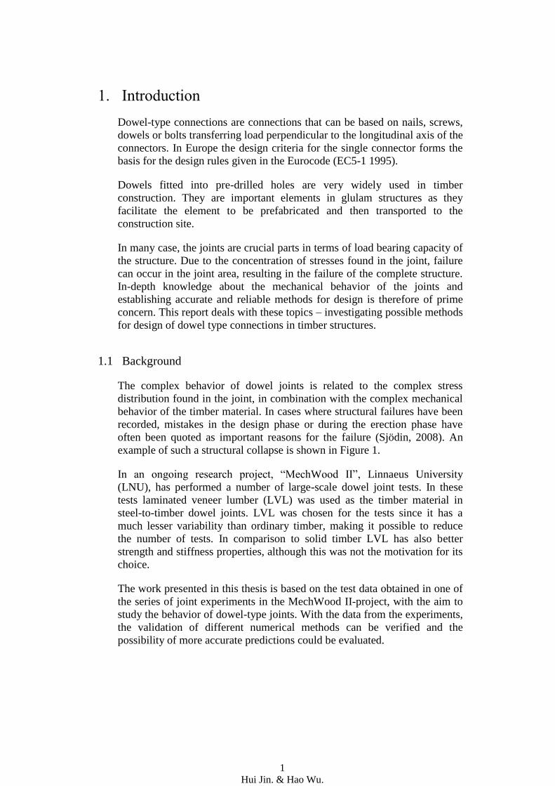
1. Introduction
Dowel-type connections are connections that can be based on nails, screws,
dowels or bolts transferring load perpendicular to the longitudinal axis of the
connectors. In Europe the design criteria for the single connector forms the
basis for the design rules given in the Eurocode (EC5-1 1995).
Dowels fitted into pre-drilled holes are very widely used in timber
construction. They are important elements in glulam structures as they
facilitate the element to be prefabricated and then transported to the
construction site.
In many case, the joints are crucial parts in terms of load bearing capacity of
the structure. Due to the concentration of stresses found in the joint, failure
can occur in the joint area, resulting in the failure of the complete structure.
In-depth knowledge about the mechanical behavior of the joints and
establishing accurate and reliable methods for design is therefore of prime
concern. This report deals with these topics – investigating possible methods
for design of dowel type connections in timber structures.
1.1 Background
The complex behavior of dowel joints is related to the complex stress
distribution found in the joint, in combination with the complex mechanical
behavior of the timber material. In cases where structural failures have been
recorded, mistakes in the design phase or during the erection phase have
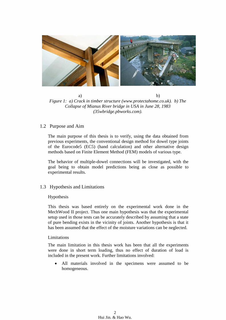
often been quoted as important reasons for the failure (Sjödin, 2008). An
example of such a structural collapse is shown in Figure 1.
In an ongoing research project, “MechWood II”, Linnaeus University
(LNU), has performed a number of large-scale dowel joint tests. In these
tests laminated veneer lumber (LVL) was used as the timber material in
steel-to-timber dowel joints. LVL was chosen for the tests since it has a
much lesser variability than ordinary timber, making it possible to reduce
the number of tests. In comparison to solid timber LVL has also better
strength and stiffness properties, although this was not the motivation for its
choice.
The work presented in this thesis is based on the test data obtained in one of
the series of joint experiments in the MechWood II-project, with the aim to
study the behavior of dowel-type joints. With the data from the experiments,
the validation of different numerical methods can be verified and the
possibility of more accurate predictions could be evaluated.
2
Hui Jin. & Hao Wu.
a) b)
Figure 1: a) Crack in timber structure (www.protectahome.co.uk). b) The
Collapse of Mianus River bridge in USA in June 28, 1983
(35wbridge.pbworks.com).
1.2 Purpose and Aim
The main purpose of this thesis is to verify, using the data obtained from
previous experiments, the conventional design method for dowel type joints
of the Eurocode5 (EC5) (hand calculation) and other alternative design
methods based on Finite Element Method (FEM) models of various type.
The behavior of multiple-dowel connections will be investigated, with the
goal being to obtain model predictions being as close as possible to
experimental results.
1.3 Hypothesis and Limitations
Hypothesis
This thesis was based entirely on the experimental work done in the
MechWood II project. Thus one main hypothesis was that the experimental
setup used in those tests can be accurately described by assuming that a state
of pure bending exists in the vicinity of joints. Another hypothesis is that it
has been assumed that the effect of the moisture variations can be neglected.
Limitations
The main limitation in this thesis work has been that all the experiments
were done in short term loading, thus no effect of duration of load is
included in the present work. Further limitations involved:
All materials involved in the specimens were assumed to be
homogeneous.
3
Hui Jin. & Hao Wu.
The constitutive relation between the stress and the strain was
restricted to linear elastic.
All mechanical properties of the timber and the dowel were taken
from literature.
1.4 Reliability, validity and objectivity
Although the EC5 design approach is widely used in structures, it is much
debated also. It is not clearly stated in EC5 how to use the design approach
e.g. in multiple dowel joint exposed to bending, leaving room for
interpretations. Thus, the validity of the design approach can be questioned,
per se. What is more, the validity of the investigations performed is limited
to the specific joint configurations investigated (materials, geometry, loading
conditions).
1.5 Literature review
A Large number of researchers have investigated the behavior of dowel type
connections over the years. The most well–known theory, which also serves
as a basis for EC5 approach is the so-called Johansen theory (Johansen,
1949). This is sometimes also referred to as the European yield model
(EYM).
The characteristic load-carrying capacity according to EC5 is illustrated in
Dorn (2012) for the case of varying several parameters such as dowel
diameter, wood density, steel quality and the connection width. Furthermore,
the study also stated how the failure modes differ due to varying connection
parameters.
In the study of Sjödin and Serrano (2008), two different methods were used
to calculate the capacity of multiple dowel joints loaded in tension parallel to
the grain: Linear Elastic Fracture Mechanics (LEFM) and the EC-5
approach.
The effect of friction was studied in Serrano et al. (2008) where
experimental results showed that the load-bearing capacity in tension
increases when rough surface dowels were used as comparison to smooth
surface dowels. The experiments confirmed the advantage of rough surface
dowels, something which not taken into account in the EC-5. However, the
experiments were done on single dowel joints in tension along the grain, and
the beneficial effect of high friction can be questioned for other joint
configurations and loadings.
Serrano and Gustafsson (2006) give an overview of various fracture
mechanics methods that could possibly be used in timber engineering
applications. At that time, fracture mechanics concepts had not been widely

4
Hui Jin. & Hao Wu.
accepted for use in timber design. Using fracture mechanics concepts make
it possible to take the fracture toughness of wood into account.
The mean stress approach was presented in the study of Sjödin and Serrano
(2008), where this numerical approach was verified to be suitable to fit the
experimental results. This approach is based on LEFM and the purpose is to
evaluate the load-carrying capacity by mean stresses that act on a certain
area instead of using the stresses in a single point.
5
Hui Jin. & Hao Wu.
2. Theory
This section discusses the mechanical properties of timber and dowels.
Several analytical and numerical models that have been proposed are
briefly described.
2.1 European yield model
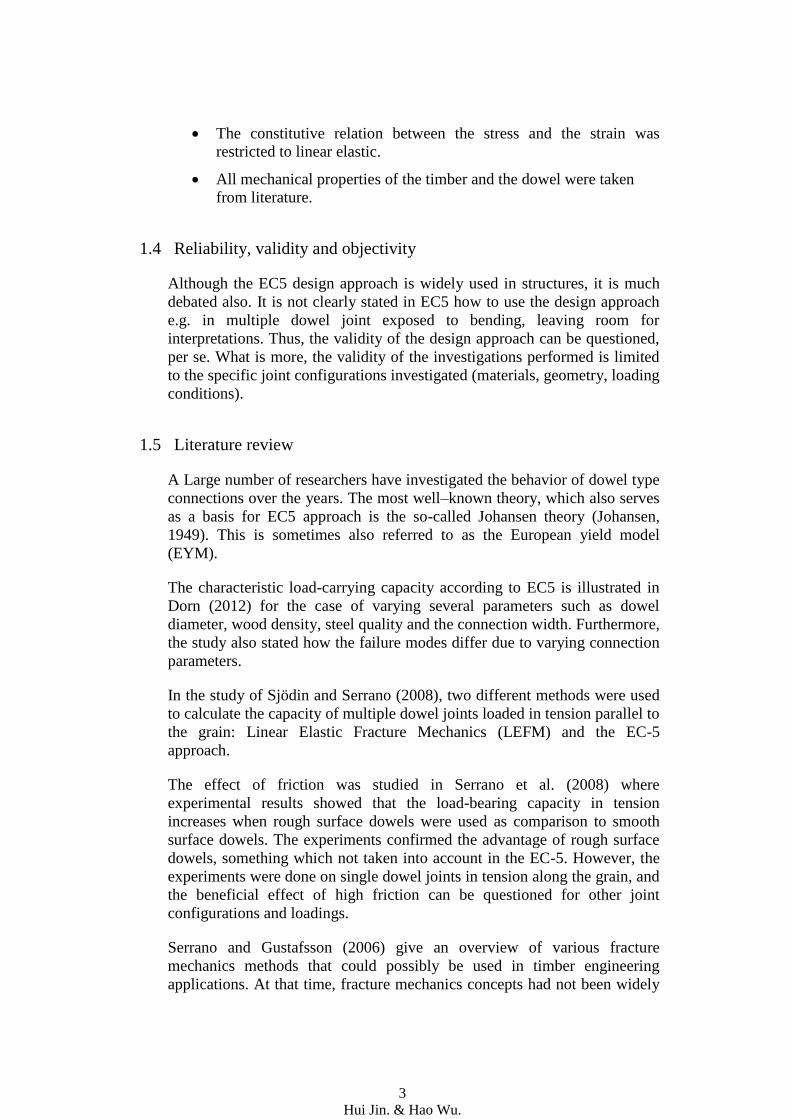
2.1.1 Dowel action
The load on the fastener is introduced by e.g. steel plates and is counteracted
by the contact pressure and possibly friction between the timber and dowel.
The dowel will work as a beam, but once deformed, the shear action can be
complemented with a tensile action in the dowel.
Figure 2: dowel action with embedding strength.
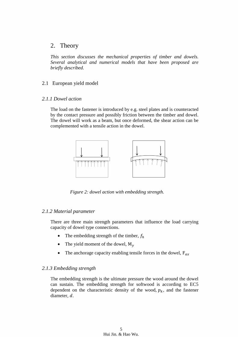
2.1.2 Material parameter
There are three main strength parameters that influence the load carrying
capacity of dowel type connections.
The embedding strength of the timber,
The yield moment of the dowel,
The anchorage capacity enabling tensile forces in the dowel,
2.1.3 Embedding strength
The embedding strength is the ultimate pressure the wood around the dowel
can sustain. The embedding strength for softwood is according to EC5
dependent on the characteristic density of the wood, , and the fastener
diameter, .
6
Hui Jin. & Hao Wu.
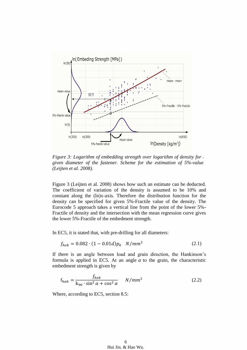
Figure 3 (Leijten et al. 2008) shows how such an estimate can be deducted.
The coefficient of variation of the density is assumed to be 10% and
constant along the (ln)x-axis. Therefore the distribution function for the
density can be specified for given 5%-Fractile value of the density. The
Eurocode 5 approach takes a vertical line from the point of the lower 5%-
Fractile of density and the intersection with the mean regression curve gives
the lower 5%-Fractile of the embedment strength.
In EC5, it is stated that, with pre-drilling for all diameters:
( ) ⁄ (2.1)
If there is an angle between load and grain direction, the Hankinson’s
formula is applied in EC5. At an angle to the grain, the characteristic
embedment strength is given by
⁄ (2.2)
Where, according to EC5, section 8.5:
Figure 3: Logarithm of embedding strength over logarithm of density for a
given diameter of the fastener. Scheme for the estimation of 5%-values
(Leijten et al. 2008).
7
Hui Jin. & Hao Wu.
(Softwoods)
(LVL)
(Hardwoods)
(2.3)
2.1.4 Yielding moment
The yielding moment is referred to as ultimate (plastic) plastic moment that
the steel dowel can withstand. The characteristic value of the yield moment
is dependent on fastener diameter and ultimate steel strength of
the dowel.
For round nails
(2.4)
For all fastener with
(2.5)
2.1.5 Slotted-in steel plate
By using steel plates, very efficient joints can be made in terms of load
bearing capacity. The main drawback using steel is related to fire. Due to the
fact that steel softens at elevated temperatures, steel plates are always
protected by fire proof paint or are covered in the structures by insulating
materials (wood, mineral wool, gypsum). Dowel holes are pre-drilled both in
wood and steel, and dowels are then inserted to complete the connection.
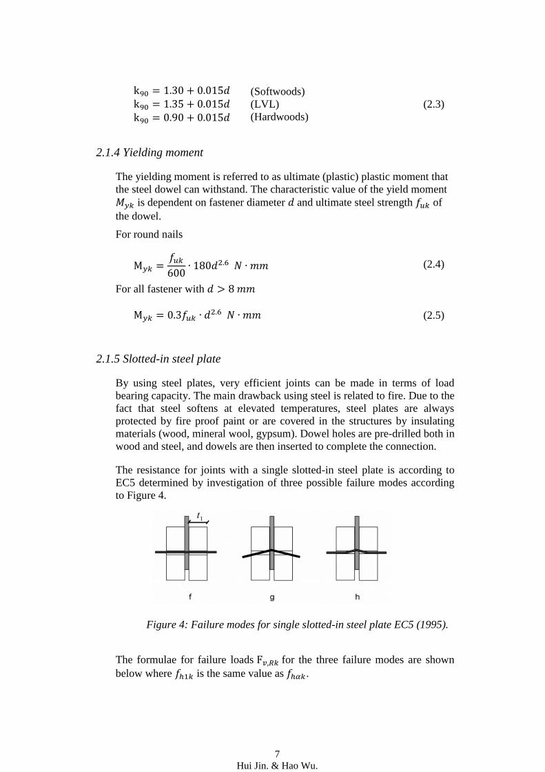
The resistance for joints with a single slotted-in steel plate is according to
EC5 determined by investigation of three possible failure modes according
to Figure 4.
Figure 4: Failure modes for single slotted-in steel plate EC5 (1995).
The formulae for failure loads for the three failure modes are shown
below where is the same value as .
8
Hui Jin. & Hao Wu.
Where d is fastener diameter and is timber thickness.
2.2 Orthotropic elasticity
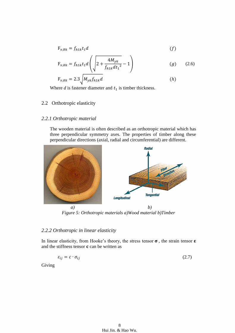
2.2.1 Orthotropic material
The wooden material is often described as an orthotropic material which has
three perpendicular symmetry axes. The properties of timber along these
perpendicular directions (axial, radial and circumferential) are different.
a) b)
Figure 5: Orthotropic materials a)Wood material b)Timber
2.2.2 Orthotropic in linear elasticity
In linear elasticity, from Hooke’s theory, the stress tensor , the strain tensor
and the stiffness tensor can be written as
(2.7)
Giving
( )
(√
) ( ) (2.6)
√ ( )
9
Hui Jin. & Hao Wu.
[ ]
[
]
[
]
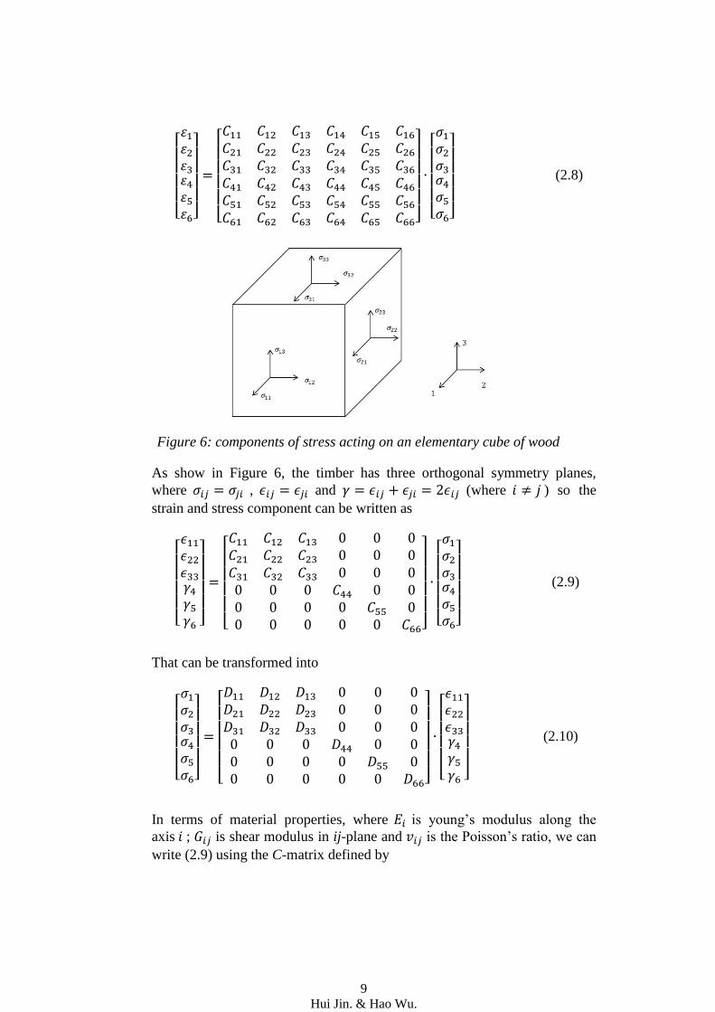
(2.8)
Figure 6: components of stress acting on an elementary cube of wood
As show in Figure 6, the timber has three orthogonal symmetry planes,
where , and (where ) so the
strain and stress component can be written as
[
]
[ ]
[
]
(2.9)
That can be transformed into
[
]
[ ]
[
]
(2.10)
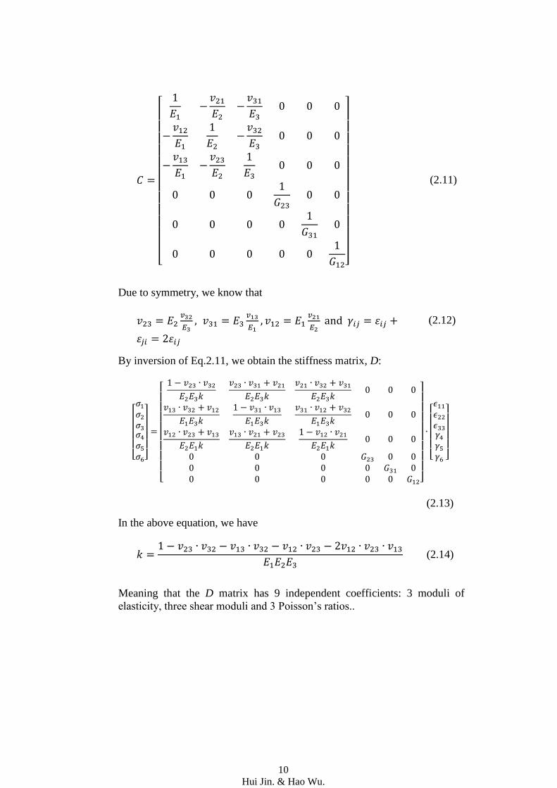
In terms of material properties, where is young’s modulus along the
axis ; is shear modulus in ij-plane and is the Poisson’s ratio, we can
write (2.9) using the C-matrix defined by
10
Hui Jin. & Hao Wu.
[
]
(2.11)
Due to symmetry, we know that
(2.12)
By inversion of Eq.2.11, we obtain the stiffness matrix, D:
[
]
[
]
[
]
(2.13)
In the above equation, we have
(2.14)
Meaning that the D matrix has 9 independent coefficients: 3 moduli of
elasticity, three shear moduli and 3 Poisson’s ratios..
11
Hui Jin. & Hao Wu.
2.3 Linear elasticity fracture mechanics
2.3.1 Linear Elastic Fracture Mechanics-LEFM
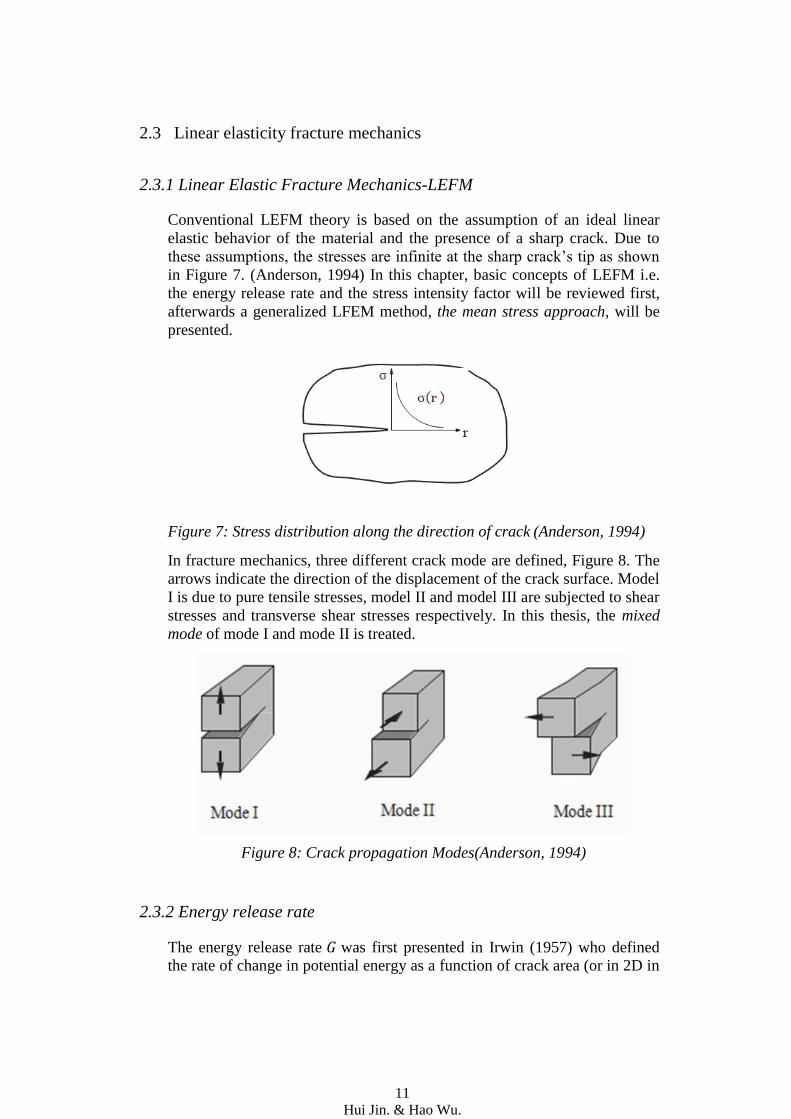
Conventional LEFM theory is based on the assumption of an ideal linear
elastic behavior of the material and the presence of a sharp crack. Due to
these assumptions, the stresses are infinite at the sharp crack’s tip as shown
in Figure 7. (Anderson, 1994) In this chapter, basic concepts of LEFM i.e.
the energy release rate and the stress intensity factor will be reviewed first,
afterwards a generalized LFEM method, the mean stress approach, will be
presented.
Figure 7: Stress distribution along the direction of crack (Anderson, 1994)
In fracture mechanics, three different crack mode are defined, Figure 8. The
arrows indicate the direction of the displacement of the crack surface. Model
I is due to pure tensile stresses, model II and model III are subjected to shear
stresses and transverse shear stresses respectively. In this thesis, the mixed
mode of mode I and mode II is treated.
Figure 8: Crack propagation Modes(Anderson, 1994)
2.3.2 Energy release rate
The energy release rate was first presented in Irwin (1957) who defined
the rate of change in potential energy as a function of crack area (or in 2D in
12
Hui Jin. & Hao Wu.
terms of crack length). If , the fracture occurs when the crack length,
a, is equal to ac:
(2.15)
Where E refers to Young s modulous, refers to applied stress, and a refers
to half length of the crack,
The failure stress is denoted . Thus the can be considered as a
material property which is independent of the geometry. As Figure 8 shows,
it is possible to separate the energy release rate G into three different modes
as .
The total energy release rate = .
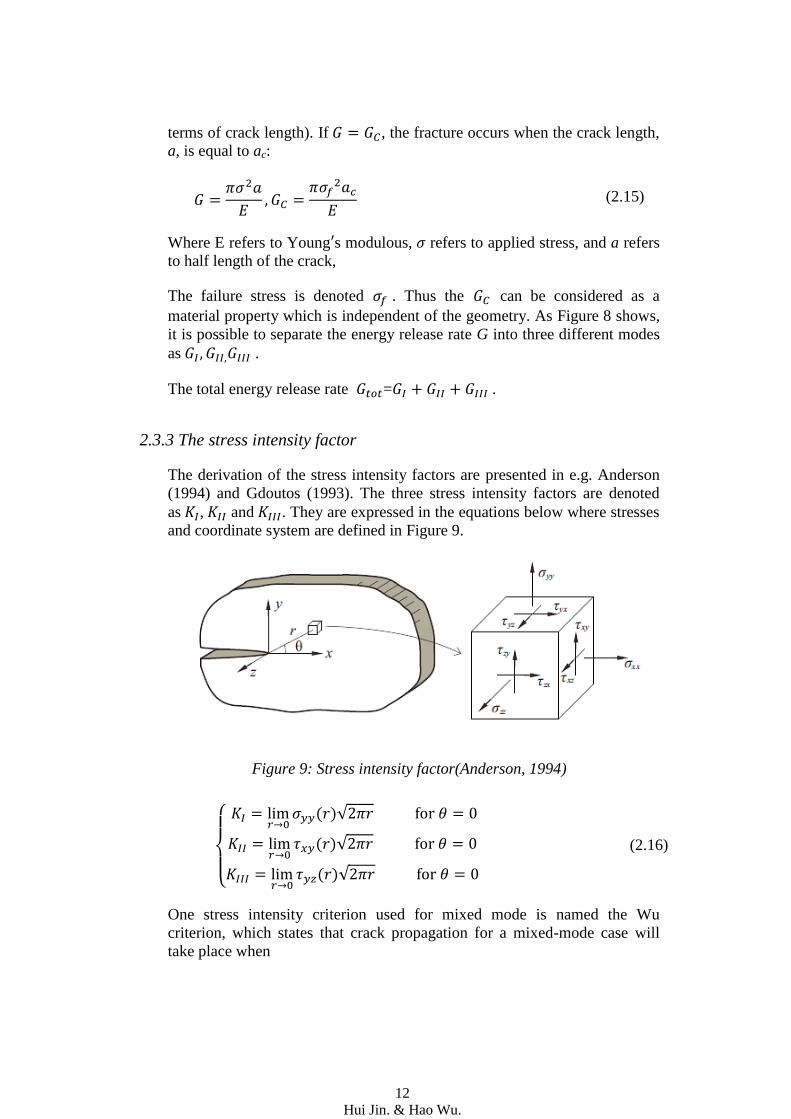
2.3.3 The stress intensity factor
The derivation of the stress intensity factors are presented in e.g. Anderson
(1994) and Gdoutos (1993). The three stress intensity factors are denoted
as , and . They are expressed in the equations below where stresses
and coordinate system are defined in Figure 9.
Figure 9: Stress intensity factor(Anderson, 1994)
{
( )√
( )√
( )√
(2.16)
One stress intensity criterion used for mixed mode is named the Wu
criterion, which states that crack propagation for a mixed-mode case will
take place when
13
Hui Jin. & Hao Wu.
(
)
(2.17)
2.3.4 Relation between G and K
The relation between stress intensity factors can be stated by the
following equations. (Blyberg, 2008)
√
(2.18) √
Where
√
√
(2.19)
√
√
(2.20)
Note: are the Young’s moduli of the orthotropic material in the different
directions, is the shear modulus and is Poisson’s ratio.
2.3.5 Mean stress approach-Generalized LEEM
As shown in Figure 9, the square root singularities are typically found at the
tips of sharp cracks. Conventional stress criteria are restricted to situations
without any stress singularity. In contrast, a generalized method e.g. the
mean stress method can be used no matter if the singularity exists or not.
(Serrano and Gustafsson, 2006) The basic idea of the mean stress methods is
to evaluate the average, or mean, stress over a predefined length along the
assumed crack propagation direction. The predefined length is chosen such
that the mean stress method will give the same prediction of failure load as a
standard LEFM-based method if a sharp crack exists.
The fracture criterions used for mean the stress method is given as
14
Hui Jin. & Hao Wu.
(
)
(
)
(2.21)
Where are the mean stress assumed to be acting across a possible
fracture area, is the shear strength parallel to the grain and is the tensile
strength perpendicular to the grain. This equation holds on when i.e.
the normal stress is tensile stress. If i.e. the normal stress is
compressed, only the shear stress will be taken into computation. The
crack area is calculated as the width of the timber times a certain length ( )
in the longitudinal direction. (Gustafsson, 2002), (Serrano and Gustafsson,
2006)
Using the definition of , according to the Eq.2.18, the expression
of over a certain length can be obtained
∫ ( )
√
(2.22)
∫ ( )
√
(2.23)
With insertion into Eq.2.22 and Eq.2.23 the definition of mixed mode ratio,
(2.24)
The expression of the mean stress length can be obtained,
(
)
{
√ √
}
( ⁄ )
(2.25)
Where
√
√ √
(2.26)
And the mean stress length can thus be calculated for any value of mixed
mode, k. Moreover we obtain
15
Hui Jin. & Hao Wu.
For pure mode I (2.27)
For pure mode II (2.28)
Assuming a certain load being applied to the body, a factor , the
critical load factor, can be calculated:
(2.29)
And the critical mean stresses are found to be
(2.30)
Or directly from the Norris criterion:
√(
)
(
)
(2.31)
2.4 The finite element method (FEM) and XFEM
Nowadays, the FEM is one of the most powerful and widely used methods
to solve arbitrary differential equations. The general steps to set up the FE
equations in elasticity are briefly outlined below. At the same time, XFEM
which is a numerical method that enhances the conventional FEM approach
by allowing discontinuous approximating functions to describe cracks, will
be introduced as well.
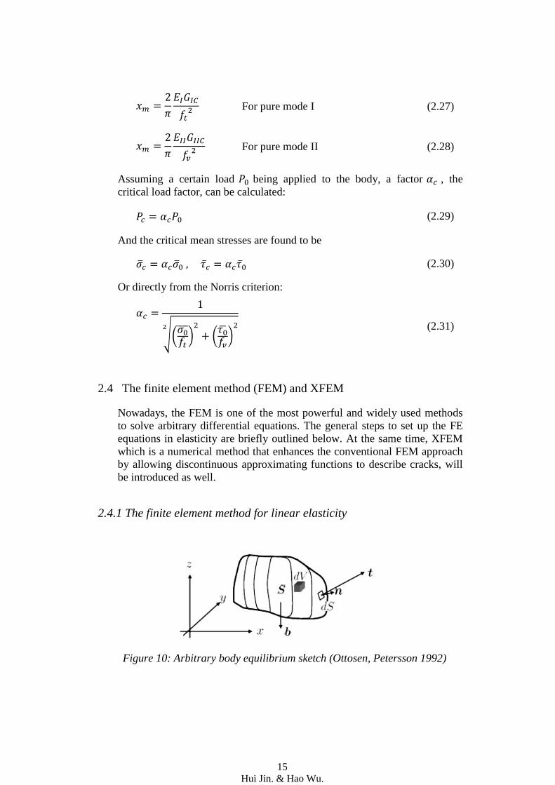
2.4.1 The finite element method for linear elasticity
Figure 10: Arbitrary body equilibrium sketch (Ottosen, Petersson 1992)
16
Hui Jin. & Hao Wu.
As shown in Figure 10Error! Reference source not found., the forces
acting on an arbitrary body is given by traction vector t over the boundary S
and the body force b in the region V. The equilibrium can be expressed as.
∫
∫
0 (2.32)
And
[
] [
] [
] (2.33)
With the following definitions
[
]
[
]
(2.34)
and Gauss’ divergence theorem, the weak formulation of the force
equilibrium can eventually be expressed as
∫ ( )
=∫
∫
(2.35)
where v is an arbitrary weight function. The finite element method
approximates the real solution by dividing the body into a number of
elements. During this procedure, the so-called shape functions are used to
approximate within each element the displacement field. The shape
functions are written as in terms of displacements, denoted by u. The
stresses and strains are denoted and . The shape functions, N, are defined
by:
u=[
]=[
]
[
]
= (2.36)
With the constitutive relation and using the Galerkin method (meaning we
use the same shape functions for the weight function as for the
approximation of the displacement):
17
Hui Jin. & Hao Wu.
= u, where =
[
]
(2.37)
and expressing the weight function as:
(2.38)
The FE formulation can be obtained
∫
∫
∫
(2.39)
Eq.2.39 was obtained at the element level, and the global parameters can be
obtained by adding all element contributions in the assembling process. The
system of equations can then be solved.
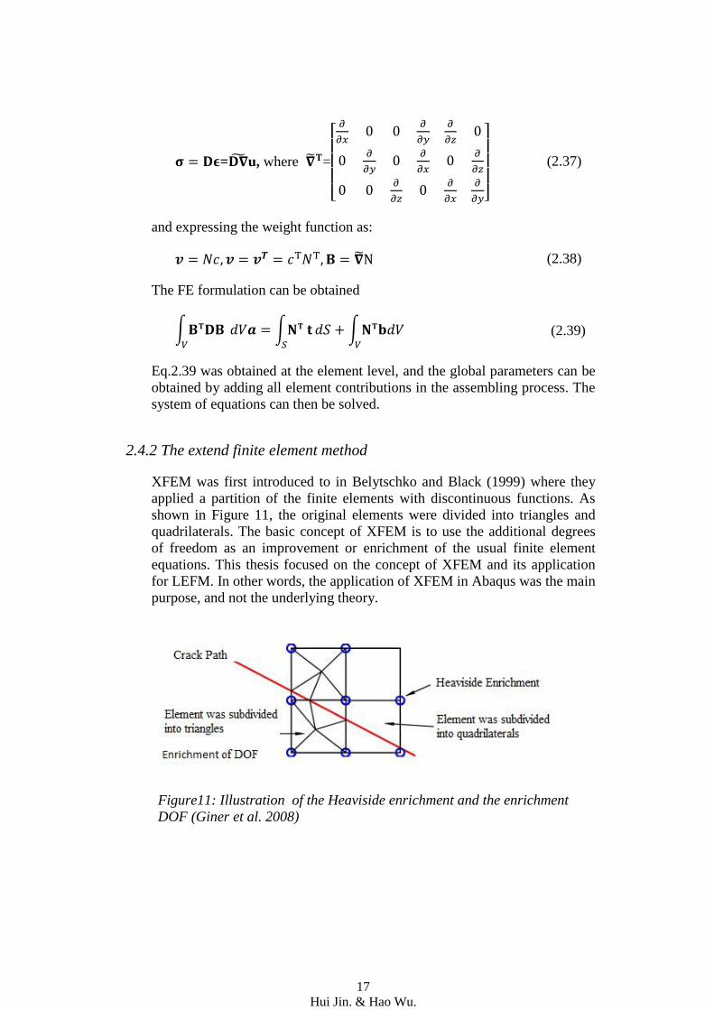
2.4.2 The extend finite element method
XFEM was first introduced to in Belytschko and Black (1999) where they
applied a partition of the finite elements with discontinuous functions. As
shown in Figure 11, the original elements were divided into triangles and
quadrilaterals. The basic concept of XFEM is to use the additional degrees
of freedom as an improvement or enrichment of the usual finite element
equations. This thesis focused on the concept of XFEM and its application
for LEFM. In other words, the application of XFEM in Abaqus was the main
purpose, and not the underlying theory.
Figure11: Illustration of the Heaviside enrichment and the enrichment
DOF (Giner et al. 2008)
18
Hui Jin. & Hao Wu.
3. Methodology
In the present chapter, the experimental setup, specimens and equipment are
described. The numerical model established to compare the results of
experiments with the FE-results is presented.
3.1 Experimental set up and data collection
3.1.1 The experimental sets up
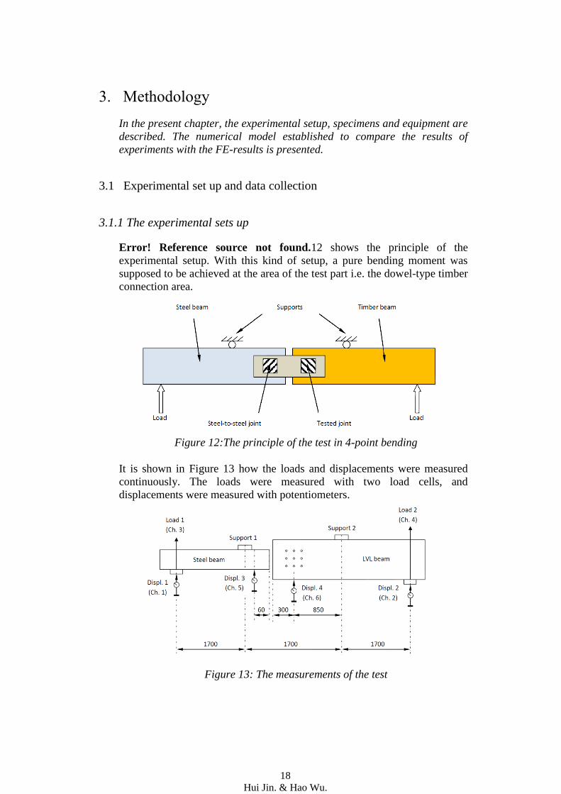
Error! Reference source not found.12 shows the principle of the
experimental setup. With this kind of setup, a pure bending moment was
supposed to be achieved at the area of the test part i.e. the dowel-type timber
connection area.
Figure 12:The principle of the test in 4-point bending
It is shown in Figure 13 how the loads and displacements were measured
continuously. The loads were measured with two load cells, and
displacements were measured with potentiometers.
Figure 13: The measurements of the test
19
Hui Jin. & Hao Wu.
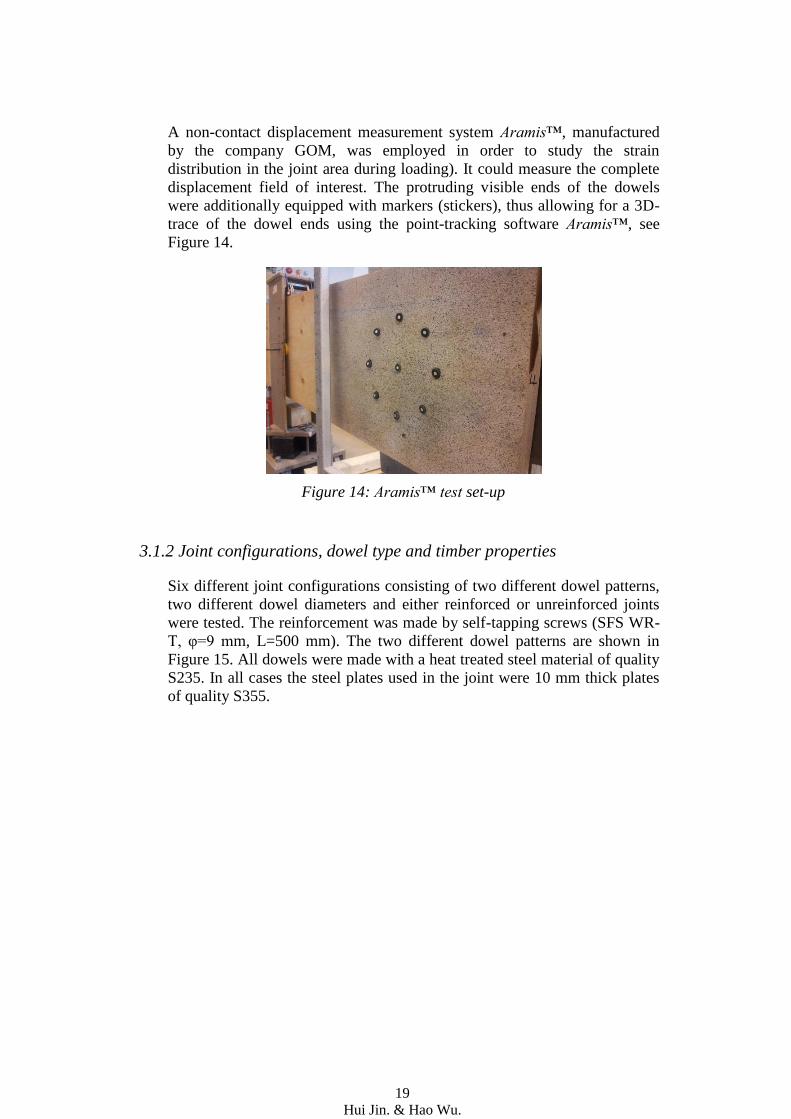
A non-contact displacement measurement system Aramis™, manufactured
by the company GOM, was employed in order to study the strain
distribution in the joint area during loading). It could measure the complete
displacement field of interest. The protruding visible ends of the dowels
were additionally equipped with markers (stickers), thus allowing for a 3D-
trace of the dowel ends using the point-tracking software Aramis™, see
Figure 14.
Figure 14: Aramis™ test set-up
3.1.2 Joint configurations, dowel type and timber properties
Six different joint configurations consisting of two different dowel patterns,
two different dowel diameters and either reinforced or unreinforced joints
were tested. The reinforcement was made by self-tapping screws (SFS WR-
T, φ=9 mm, L=500 mm). The two different dowel patterns are shown in
Figure 15. All dowels were made with a heat treated steel material of quality
S235. In all cases the steel plates used in the joint were 10 mm thick plates
of quality S355.

20
Hui Jin. & Hao Wu.
a) b)
Figure 15: Rectangular and Circular dowel pattern, a)Rectangular dowel
pattern, b) Circular dowel pattern
The timber beams are made of laminated veneer lumber (LVL, brand name
is Kerto-S®. Two LVL beams with a 12 mm Oriented Strand Board (OSB)
in between were manufactured for each test specimen. The LVL-beam is
shown in Figure 16.
Figure 16: Views of timber with the geometric size
The moduli of elasticity (MOE) for the LVL was assumed to be 13 800
MPa, 430 MPa and 130 MPa. The MOE-value for the OSB is
3 800 MPa and for the steel 210 000 MPa.
3.2 FE-models
The FE software ABAQUS, version 6.13-2 (ABAQUS Inc. (2013)) was
used for all simulations. Here a number of FE-models are described. These
are denoted Model A-E, with the following basic characteristics and linear
elastic material is used for all models.
Model A: 2D-plane stress, dowels are modeled as analytical rigid,
variations of different parameters are based on this model;
Model B: 2D-plane stress, steel plate is included, dowels are rigid;
21
Hui Jin. & Hao Wu.
Model C: 2D-plane stress, dowels are modeled as deformable;
Model D: 2D-plane stress, dowels are rigid, XFEM is used, four
cases based on this model are studied;
Model E: 3D-stress model, three sub-models based on this are
created.
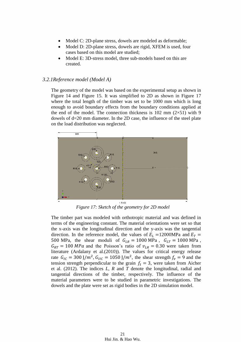
3.2.1Reference model (Model A)
The geometry of the model was based on the experimental setup as shown in
Figure 14 and Figure 15. It was simplified to 2D as shown in Figure 17
where the total length of the timber was set to be 1000 mm which is long
enough to avoid boundary effects from the boundary conditions applied at
the end of the model. The connection thickness is 102 mm (2×51) with 9
dowels of d=20 mm diameter. In the 2D case, the influence of the steel plate
on the load distribution was neglected.
Figure 17: Sketch of the geometry for 2D model
The timber part was modeled with orthotropic material and was defined in
terms of the engineering constant. The material orientations were set so that
the x-axis was the longitudinal direction and the y-axis was the tangential
direction. In the reference model, the values of 12000MPa and MPa, the shear moduli of , ,
and the Poisson’s ratio of were taken from
literature (Ardalany et al.(2010)). The values for critical energy release
rate , the shear strength and the
tension strength perpendicular to the grain , were taken from Aicher
et al. (2012). The indices L, R and T denote the longitudinal, radial and
tangential directions of the timber, respectively. The influence of the
material parameters were to be studied in parametric investigations. The
dowels and the plate were set as rigid bodies in the 2D simulation model.
22
Hui Jin. & Hao Wu.
The contact behavior between dowel and timber was defined in terms of
normal behavior (hard contact) and tangential behavior (setting the frictional
coefficient). The initial coefficient of friction was set to 0.1.
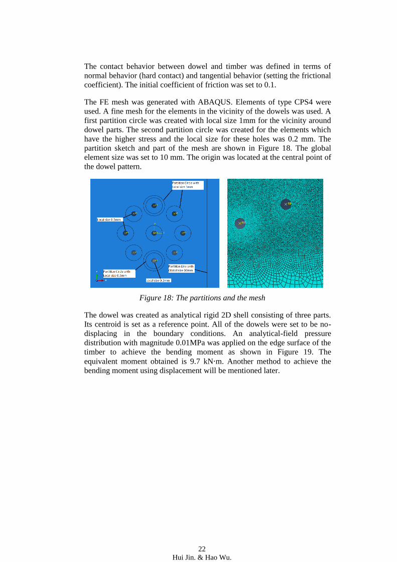
The FE mesh was generated with ABAQUS. Elements of type CPS4 were
used. A fine mesh for the elements in the vicinity of the dowels was used. A
first partition circle was created with local size 1mm for the vicinity around
dowel parts. The second partition circle was created for the elements which
have the higher stress and the local size for these holes was 0.2 mm. The
partition sketch and part of the mesh are shown in Figure 18. The global
element size was set to 10 mm. The origin was located at the central point of
the dowel pattern.
Figure 18: The partitions and the mesh
The dowel was created as analytical rigid 2D shell consisting of three parts.
Its centroid is set as a reference point. All of the dowels were set to be no-
displacing in the boundary conditions. An analytical-field pressure
distribution with magnitude 0.01MPa was applied on the edge surface of the
timber to achieve the bending moment as shown in Figure 19. The
equivalent moment obtained is 9.7 kN m. Another method to achieve the
bending moment using displacement will be mentioned later.
23
Hui Jin. & Hao Wu.
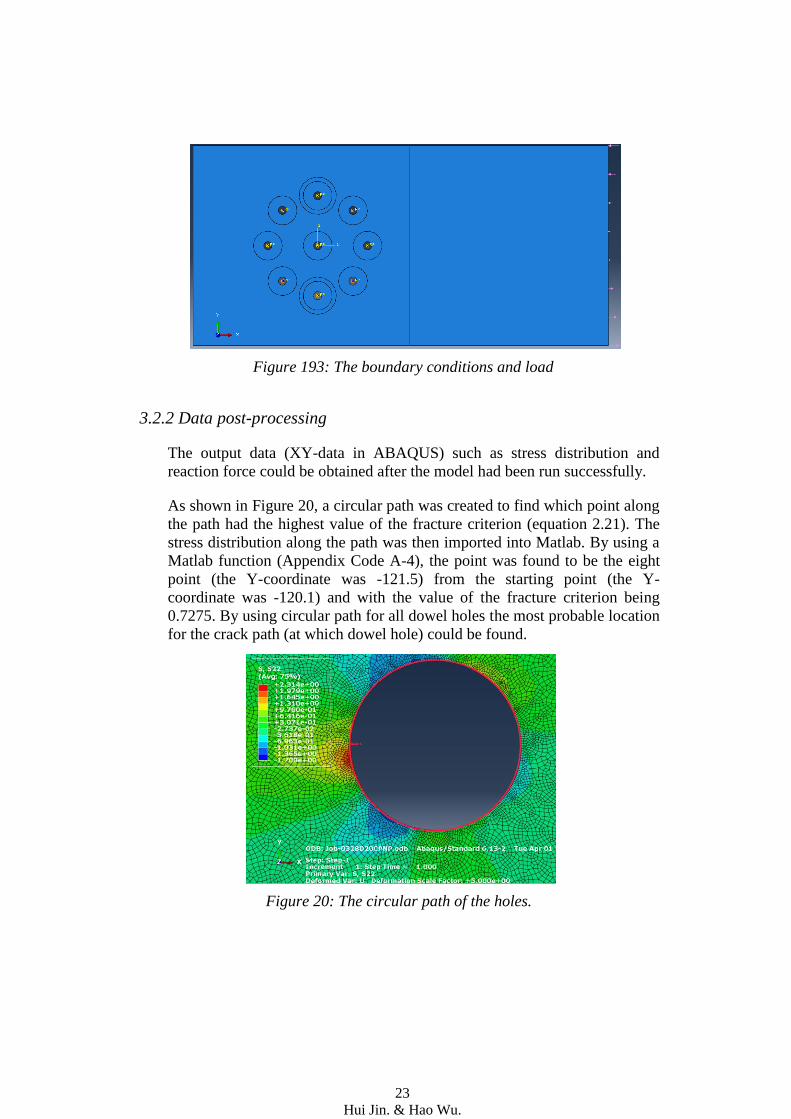
Figure 193: The boundary conditions and load
3.2.2 Data post-processing
The output data (XY-data in ABAQUS) such as stress distribution and
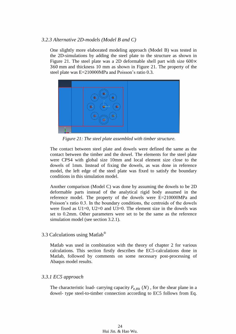
reaction force could be obtained after the model had been run successfully.
As shown in Figure 20, a circular path was created to find which point along
the path had the highest value of the fracture criterion (equation 2.21). The
stress distribution along the path was then imported into Matlab. By using a
Matlab function (Appendix Code A-4), the point was found to be the eight
point (the Y-coordinate was -121.5) from the starting point (the Y-
coordinate was -120.1) and with the value of the fracture criterion being
0.7275. By using circular path for all dowel holes the most probable location
for the crack path (at which dowel hole) could be found.
Figure 20: The circular path of the holes.
24
Hui Jin. & Hao Wu.
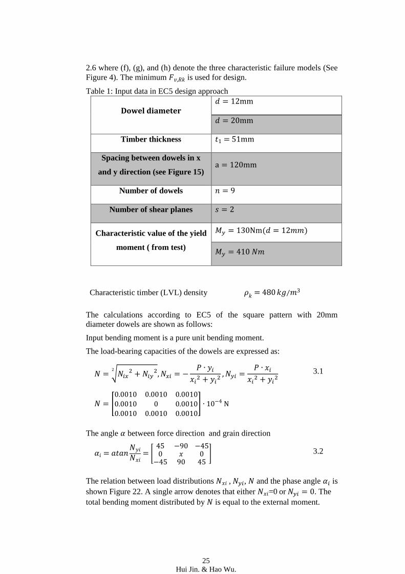
3.2.3 Alternative 2D-models (Model B and C)
One slightly more elaborated modeling approach (Model B) was tested in
the 2D-simulations by adding the steel plate to the structure as shown in
Figure 21. The steel plate was a 2D deformable shell part with size 600 and thickness 10 mm as shown in Figure 21. The property of the
steel plate was E=210000MPa and Poisson’s ratio 0.3.
Figure 21: The steel plate assembled with timber structure.
The contact between steel plate and dowels were defined the same as the
contact between the timber and the dowel. The elements for the steel plate
were CPS4 with global size 10mm and local element size close to the
dowels of 1mm. Instead of fixing the dowels, as was done in reference
model, the left edge of the steel plate was fixed to satisfy the boundary
conditions in this simulation model.
Another comparison (Model C) was done by assuming the dowels to be 2D
deformable parts instead of the analytical rigid body assumed in the
reference model. The property of the dowels were E=210000MPa and
Poisson’s ratio 0.3. In the boundary conditions, the centroids of the dowels
were fixed as U1=0, U2=0 and U3=0. The element size in the dowels was
set to 0.2mm. Other parameters were set to be the same as the reference
simulation model (see section 3.2.1).
3.3 Calculations using Matlab®
Matlab was used in combination with the theory of chapter 2 for various
calculations. This section firstly describes the EC5-calculations done in
Matlab, followed by comments on some necessary post-processing of
Abaqus model results.
3.3.1 EC5 approach
The characteristic load- carrying capacity ( ) , for the shear plane in a
dowel- type steel-to-timber connection according to EC5 follows from Eq.
25
Hui Jin. & Hao Wu.
2.6 where (f), (g), and (h) denote the three characteristic failure models (See
Figure 4). The minimum is used for design.
Table 1: Input data in EC5 design approach
Dowel diameter
Timber thickness
Spacing between dowels in x
and y direction (see Figure 15)
Number of dowels
Number of shear planes
Characteristic value of the yield
moment ( from test)
( )
Characteristic timber (LVL) density ⁄
The calculations according to EC5 of the square pattern with 20mm
diameter dowels are shown as follows:
Input bending moment is a pure unit bending moment.
The load-bearing capacities of the dowels are expressed as:
√
3.1
[
]
The angle between force direction and grain direction
[
] 3.2
The relation between load distributions , , and the phase angle is
shown Figure 22. A single arrow denotes that either =0 or . The
total bending moment distributed by is equal to the external moment.
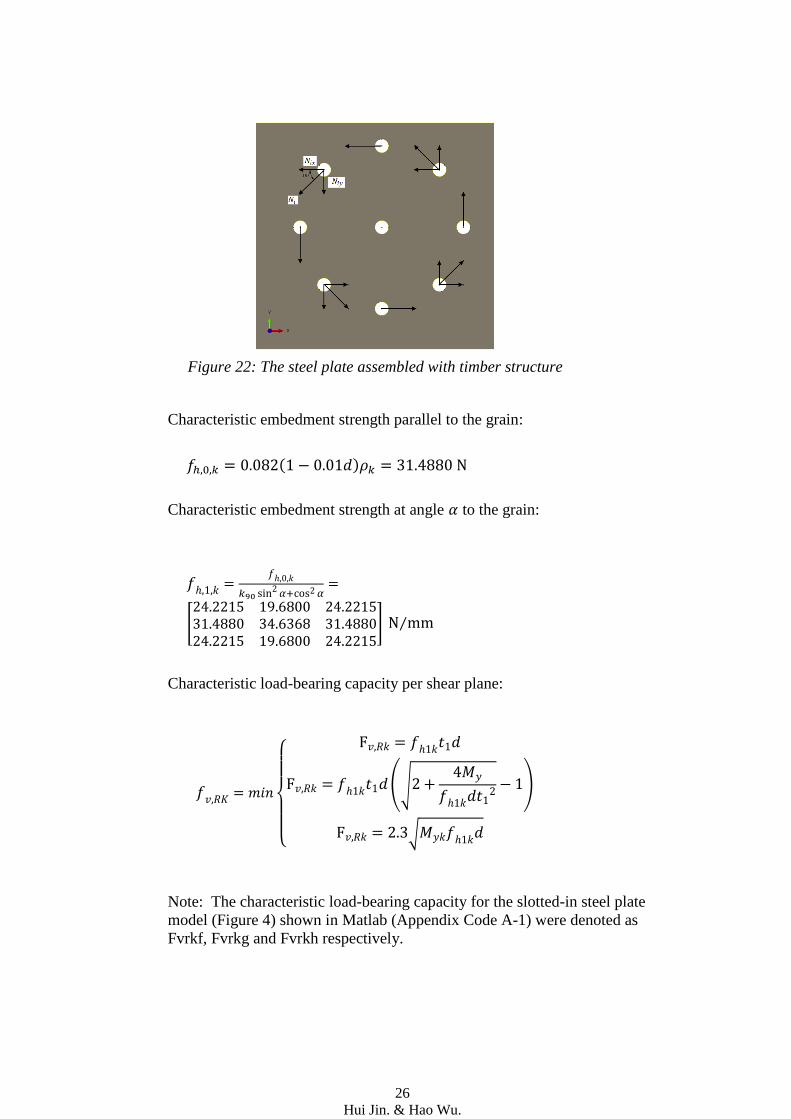
26
Hui Jin. & Hao Wu.
Figure 22: The steel plate assembled with timber structure
Characteristic embedment strength parallel to the grain:
( )
Characteristic embedment strength at angle to the grain:
[
] ⁄
Characteristic load-bearing capacity per shear plane:
{
(√
)
√
Note: The characteristic load-bearing capacity for the slotted-in steel plate
model (Figure 4) shown in Matlab (Appendix Code A-1) were denoted as
Fvrkf, Fvrkg and Fvrkh respectively.
27
Hui Jin. & Hao Wu.
[
] ( ) 3.3
Characteristic load-bearing capacity:
⁄
[ ] 3.4
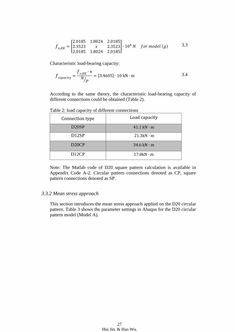
According to the same theory, the characteristic load-bearing capacity of
different connections could be obtained (Table 2).
Table 2: load capacity of different connections
Connection type Load capacity
D20SP
D12SP
D20CP
D12CP
Note: The Matlab code of D20 square pattern calculation is available in
Appendix Code A-2. Circular pattern connections denoted as CP, square
pattern connections denoted as SP.
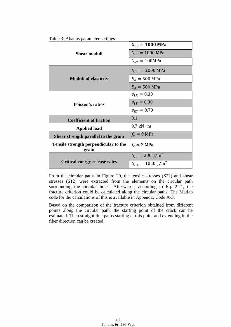
3.3.2 Mean stress approach
This section introduces the mean stress approach applied on the D20 circular
pattern. Table 3 shows the parameter settings in Abaqus for the D20 circular
pattern model (Model A).
28
Hui Jin. & Hao Wu.
Table 3: Abaqus parameter settings
Shear moduli
Moduli of elasticity
Poisson’s ratios
Coefficient of friction 0.1
Applied load
Shear strength parallel to the grain
Tensile strength perpendicular to the
grain
Critical energy release rates
⁄
⁄
From the circular paths in Figure 20, the tensile stresses (S22) and shear
stresses (S12) were extracted from the elements on the circular path
surrounding the circular holes. Afterwards, according to Eq. 2.21, the
fracture criterion could be calculated along the circular paths. The Matlab
code for the calculations of this is available in Appendix Code A-3.
Based on the comparison of the fracture criterion obtained from different
points along the circular path, the starting point of the crack can be
estimated. Then straight line paths starting at this point and extending in the
fiber direction can be created.
29
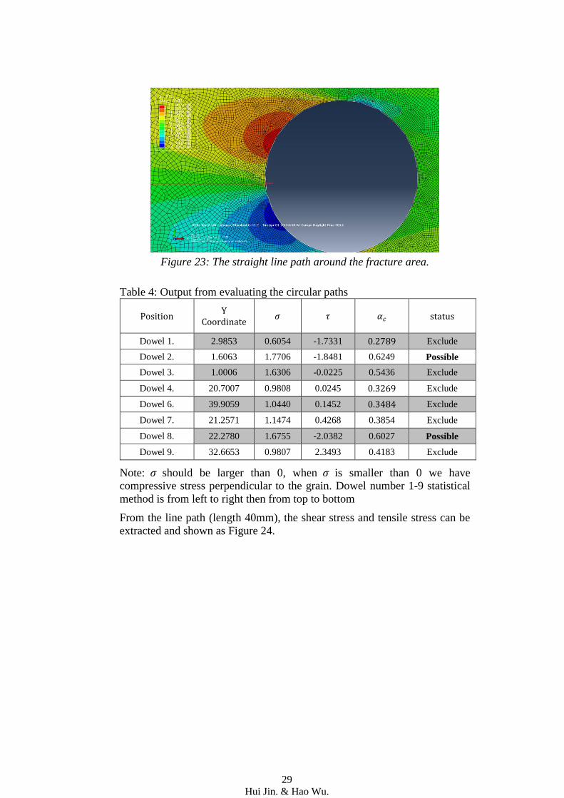
Hui Jin. & Hao Wu.
Figure 23: The straight line path around the fracture area.
Table 4: Output from evaluating the circular paths
Position Y
Coordinate status
Dowel 1. 2.9853 0.6054 -1.7331 Exclude
Dowel 2. 1.6063 1.7706 -1.8481 0.6249 Possible
Dowel 3. 1.0006 1.6306 -0.0225 0.5436 Exclude
Dowel 4. 20.7007 0.9808 0.0245 Exclude
Dowel 6. 39.9059 1.0440 0.1452 Exclude
Dowel 7. 21.2571 1.1474 0.4268 0.3854 Exclude
Dowel 8. 22.2780 1.6755 -2.0382 0.6027 Possible
Dowel 9. 32.6653 0.9807 2.3493 0.4183 Exclude
Note: should be larger than 0, when is smaller than 0 we have
compressive stress perpendicular to the grain. Dowel number 1-9 statistical
method is from left to right then from top to bottom
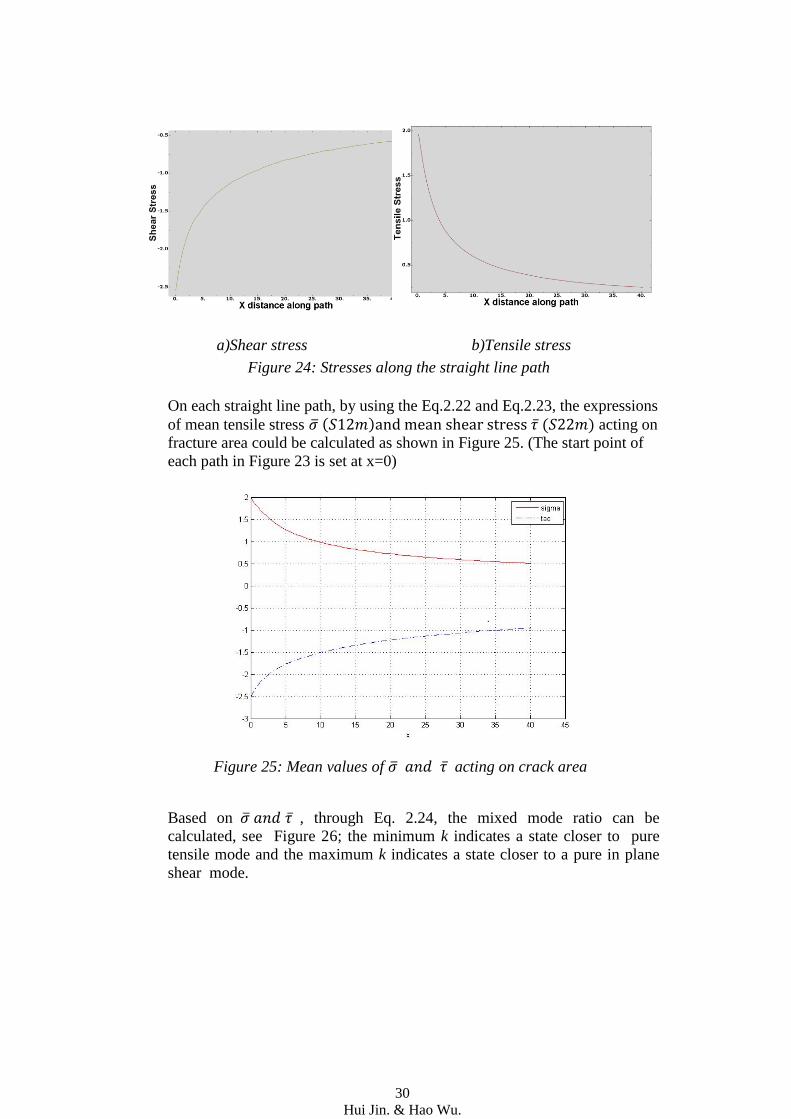
From the line path (length 40mm), the shear stress and tensile stress can be
extracted and shown as Figure 24.
30
Hui Jin. & Hao Wu.
a)Shear stress b)Tensile stress
Figure 24: Stresses along the straight line path
On each straight line path, by using the Eq.2.22 and Eq.2.23, the expressions
of mean tensile stress ( ) ( ) acting on
fracture area could be calculated as shown in Figure 25. (The start point of
each path in Figure 23 is set at x=0)
Figure 25: Mean values of acting on crack area
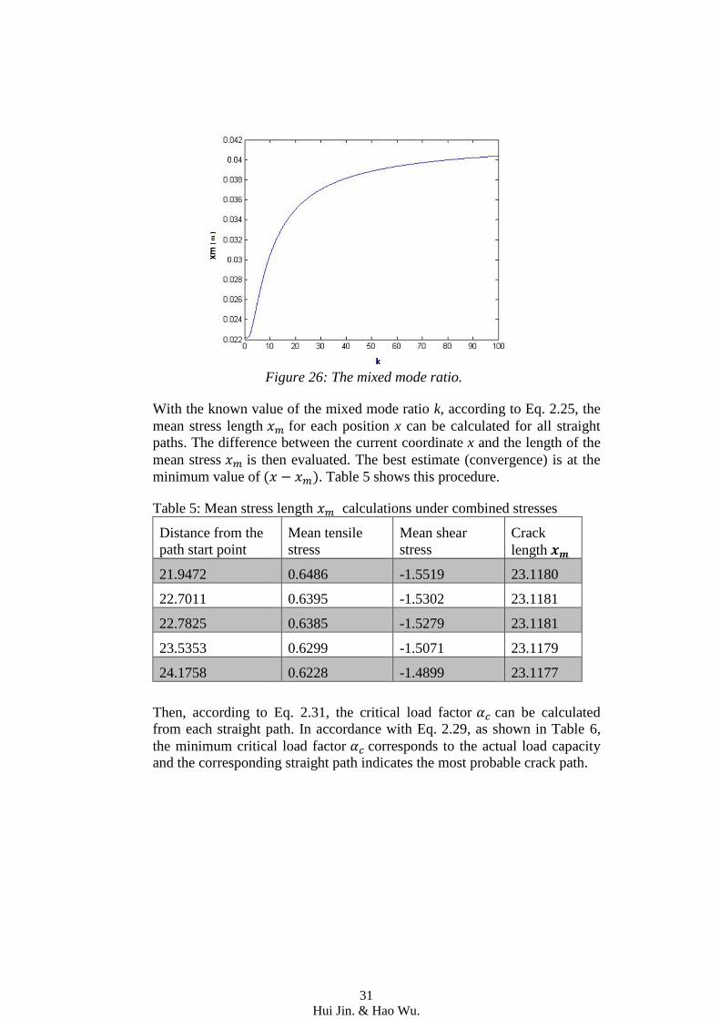
Based on , through Eq. 2.24, the mixed mode ratio can be
calculated, see Figure 26; the minimum k indicates a state closer to pure
tensile mode and the maximum k indicates a state closer to a pure in plane
shear mode.
31
Hui Jin. & Hao Wu.
Figure 26: The mixed mode ratio.
With the known value of the mixed mode ratio k, according to Eq. 2.25, the
mean stress length for each position x can be calculated for all straight
paths. The difference between the current coordinate x and the length of the
mean stress is then evaluated. The best estimate (convergence) is at the
minimum value of ( ). Table 5 shows this procedure.
Table 5: Mean stress length calculations under combined stresses
Distance from the
path start point
Mean tensile
stress
Mean shear
stress
Crack
length
21.9472 0.6486 -1.5519 23.1180
22.7011 0.6395 -1.5302 23.1181
22.7825 0.6385 -1.5279 23.1181
23.5353 0.6299 -1.5071 23.1179
24.1758 0.6228 -1.4899 23.1177
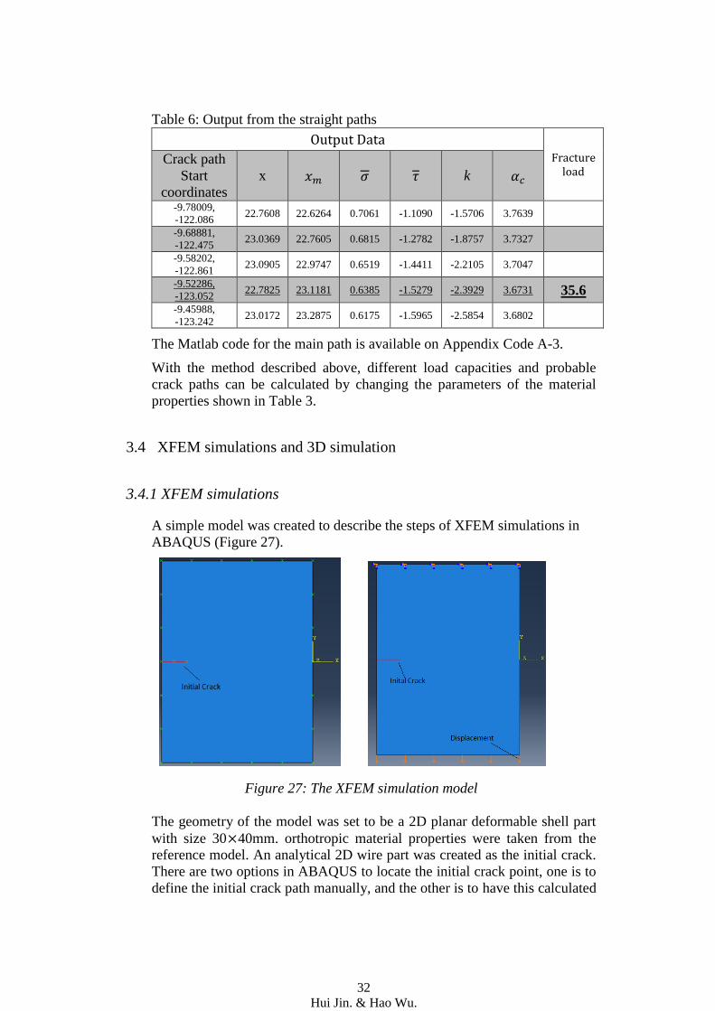
Then, according to Eq. 2.31, the critical load factor can be calculated
from each straight path. In accordance with Eq. 2.29, as shown in Table 6,
the minimum critical load factor corresponds to the actual load capacity
and the corresponding straight path indicates the most probable crack path.
32
Hui Jin. & Hao Wu.
Table 6: Output from the straight paths
Output Data Fracture
load Crack path
Start
coordinates
x k
-9.78009,
-122.086 22.7608 22.6264 0.7061 -1.1090 -1.5706 3.7639
-9.68881,
-122.475 23.0369 22.7605 0.6815 -1.2782 -1.8757 3.7327
-9.58202,
-122.861 23.0905 22.9747 0.6519 -1.4411 -2.2105 3.7047
-9.52286,
-123.052 22.7825 23.1181 0.6385 -1.5279 -2.3929 3.6731 35.6
-9.45988,
-123.242 23.0172 23.2875 0.6175 -1.5965 -2.5854 3.6802
The Matlab code for the main path is available on Appendix Code A-3.
With the method described above, different load capacities and probable
crack paths can be calculated by changing the parameters of the material
properties shown in Table 3.
3.4 XFEM simulations and 3D simulation
3.4.1 XFEM simulations
A simple model was created to describe the steps of XFEM simulations in
ABAQUS (Figure 27).
Figure 27: The XFEM simulation model
The geometry of the model was set to be a 2D planar deformable shell part
with size 30 40mm. orthotropic material properties were taken from the
reference model. An analytical 2D wire part was created as the initial crack.
There are two options in ABAQUS to locate the initial crack point, one is to
define the initial crack path manually, and the other is to have this calculated
33
Hui Jin. & Hao Wu.
automatically by ABAQUS. The first one was chosen for this simulation
model. The initial crack defines the elements which would separate during
the start of the analysis.
For the orthotropic material, a quadratic stress interaction (the “Quadsˮ for
“Traction Separation Law ˮ which is similar to (2.21)) was used for the
initiation criterion. The damage evolution is based on a power law, with
normal mode fracture energy 300 ⁄ and shear mode fracture energy
1050 ⁄ .
The interaction property was set with hard contact in normal behavior and
penalty of tangential behavior. Elements of type CPS4 were used with size
0.3 0.3mm.
A uniform displacement load u2= -1 was applied on the bottom surface and
the top surface was fixed.
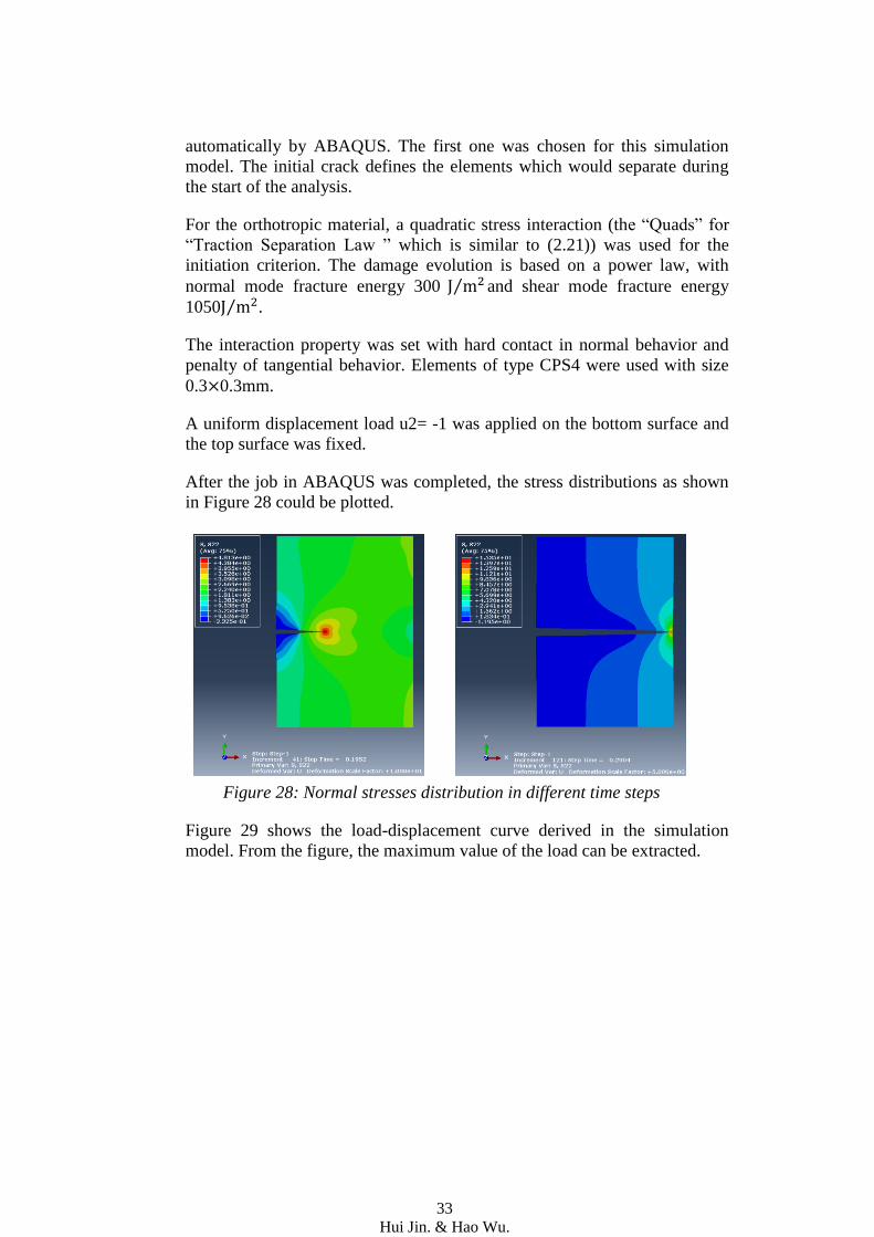
After the job in ABAQUS was completed, the stress distributions as shown
in Figure 28 could be plotted.
Figure 28: Normal stresses distribution in different time steps
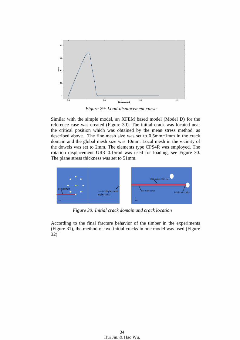
Figure 29 shows the load-displacement curve derived in the simulation
model. From the figure, the maximum value of the load can be extracted.
34
Hui Jin. & Hao Wu.
Figure 29: Load-displacement curve
Similar with the simple model, an XFEM based model (Model D) for the
reference case was created (Figure 30). The initial crack was located near
the critical position which was obtained by the mean stress method, as
described above. The fine mesh size was set to 0.5mm~1mm in the crack
domain and the global mesh size was 10mm. Local mesh in the vicinity of
the dowels was set to 2mm. The elements type CPS4R was employed. The
rotation displacement UR3=0.15rad was used for loading, see Figure 30.
The plane stress thickness was set to 51mm.
Figure 30: Initial crack domain and crack location
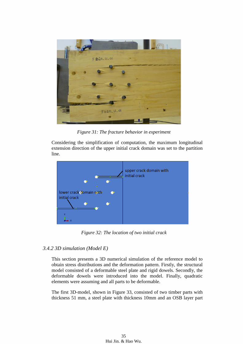
According to the final fracture behavior of the timber in the experiments
(Figure 31), the method of two initial cracks in one model was used (Figure
32).
35
Hui Jin. & Hao Wu.
Figure 31: The fracture behavior in experiment
Considering the simplification of computation, the maximum longitudinal
extension direction of the upper initial crack domain was set to the partition
line.
Figure 32: The location of two initial crack
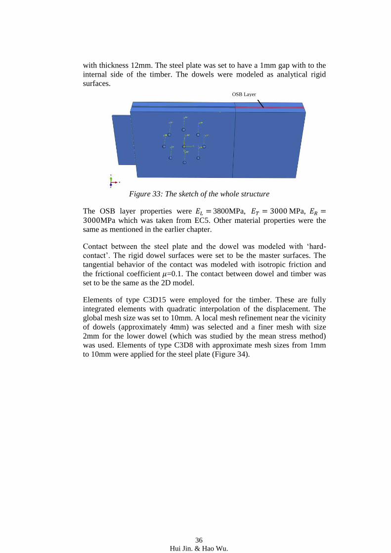
3.4.2 3D simulation (Model E)
This section presents a 3D numerical simulation of the reference model to
obtain stress distributions and the deformation pattern. Firstly, the structural
model consisted of a deformable steel plate and rigid dowels. Secondly, the
deformable dowels were introduced into the model. Finally, quadratic
elements were assuming and all parts to be deformable.
The first 3D-model, shown in Figure 33, consisted of two timber parts with
thickness 51 mm, a steel plate with thickness 10mm and an OSB layer part
36
Hui Jin. & Hao Wu.
with thickness 12mm. The steel plate was set to have a 1mm gap with to the
internal side of the timber. The dowels were modeled as analytical rigid
surfaces.
Figure 33: The sketch of the whole structure
The OSB layer properties were 3800MPa, MPa, MPa which was taken from EC5. Other material properties were the
same as mentioned in the earlier chapter.
Contact between the steel plate and the dowel was modeled with ‘hard-
contact’. The rigid dowel surfaces were set to be the master surfaces. The
tangential behavior of the contact was modeled with isotropic friction and
the frictional coefficient =0.1. The contact between dowel and timber was
set to be the same as the 2D model.
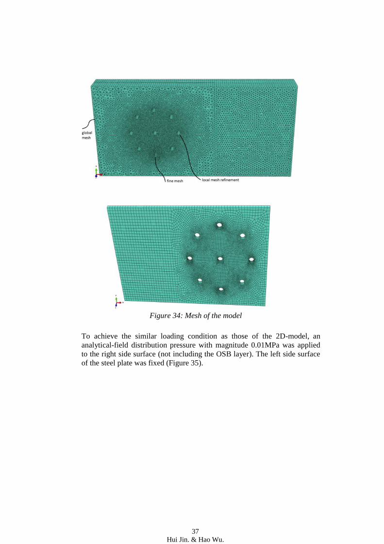
Elements of type C3D15 were employed for the timber. These are fully
integrated elements with quadratic interpolation of the displacement. The
global mesh size was set to 10mm. A local mesh refinement near the vicinity
of dowels (approximately 4mm) was selected and a finer mesh with size
2mm for the lower dowel (which was studied by the mean stress method)
was used. Elements of type C3D8 with approximate mesh sizes from 1mm
to 10mm were applied for the steel plate (Figure 34).
OSB Layer
37
Hui Jin. & Hao Wu.
Figure 34: Mesh of the model
To achieve the similar loading condition as those of the 2D-model, an
analytical-field distribution pressure with magnitude 0.01MPa was applied
to the right side surface (not including the OSB layer). The left side surface
of the steel plate was fixed (Figure 35).
38
Hui Jin. & Hao Wu.
Figure 35: Boundary conditions of the model
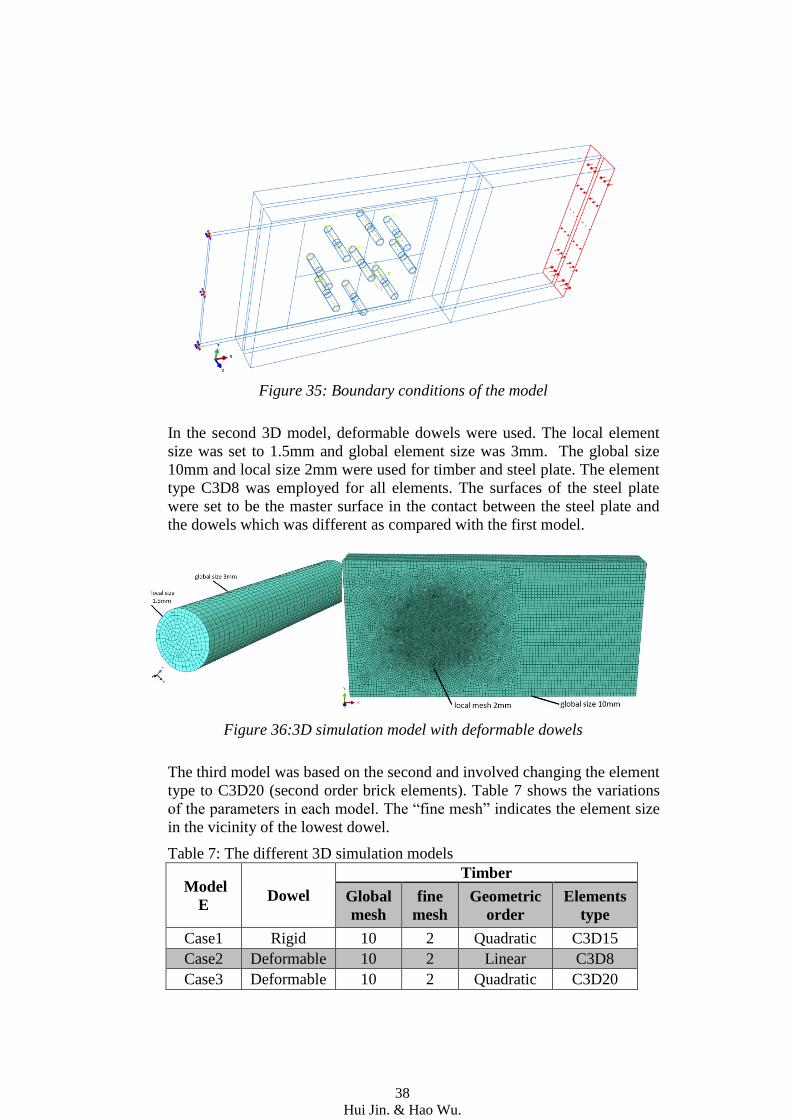
In the second 3D model, deformable dowels were used. The local element
size was set to 1.5mm and global element size was 3mm. The global size
10mm and local size 2mm were used for timber and steel plate. The element
type C3D8 was employed for all elements. The surfaces of the steel plate
were set to be the master surface in the contact between the steel plate and
the dowels which was different as compared with the first model.
Figure 36:3D simulation model with deformable dowels
The third model was based on the second and involved changing the element
type to C3D20 (second order brick elements). Table 7 shows the variations
of the parameters in each model. The “fine mesh” indicates the element size
in the vicinity of the lowest dowel.
Table 7: The different 3D simulation models
Model
E Dowel
Timber
Global
mesh
fine
mesh
Geometric
order
Elements
type
Case1 Rigid 10 2 Quadratic C3D15
Case2 Deformable 10 2 Linear C3D8
Case3 Deformable 10 2 Quadratic C3D20
39
Hui Jin. & Hao Wu.
4. Results
In this section, the results from using different approaches to calculate the
load capacity are presented and compared with the experimental results.
The aim is to understand how the various modeling approaches work.
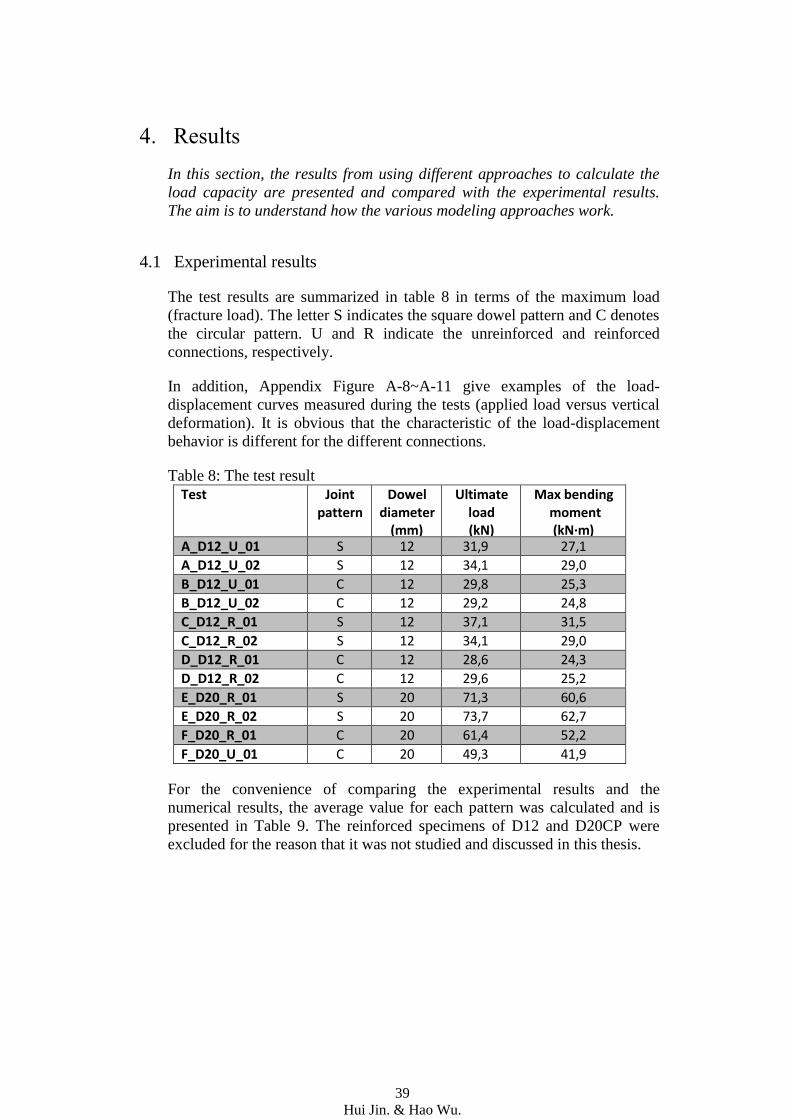
4.1 Experimental results
The test results are summarized in table 8 in terms of the maximum load
(fracture load). The letter S indicates the square dowel pattern and C denotes
the circular pattern. U and R indicate the unreinforced and reinforced
connections, respectively.
In addition, Appendix Figure A-8~A-11 give examples of the load-
displacement curves measured during the tests (applied load versus vertical
deformation). It is obvious that the characteristic of the load-displacement
behavior is different for the different connections.
Table 8: The test result
Test Joint pattern
Dowel diameter
(mm)
Ultimate load (kN)
Max bending moment (kN·m)
A_D12_U_01 S 12 31,9 27,1
A_D12_U_02 S 12 34,1 29,0
B_D12_U_01 C 12 29,8 25,3
B_D12_U_02 C 12 29,2 24,8
C_D12_R_01 S 12 37,1 31,5
C_D12_R_02 S 12 34,1 29,0
D_D12_R_01 C 12 28,6 24,3
D_D12_R_02 C 12 29,6 25,2
E_D20_R_01 S 20 71,3 60,6
E_D20_R_02 S 20 73,7 62,7
F_D20_R_01 C 20 61,4 52,2
F_D20_U_01 C 20 49,3 41,9
For the convenience of comparing the experimental results and the
numerical results, the average value for each pattern was calculated and is
presented in Table 9. The reinforced specimens of D12 and D20CP were
excluded for the reason that it was not studied and discussed in this thesis.
40
Hui Jin. & Hao Wu.
Table 9: Summary of the test result
Specimen type Joint
pattern
Dowel diameter
(mm)
Ultimate load (kN)
Max bending moment (kN m)
D20SP(R) S 20 72.5 61.7 D12SP S 12 33.0 28.1 D20CP C 20 49.3 41.9 D12CP C 12 29.5 25.1
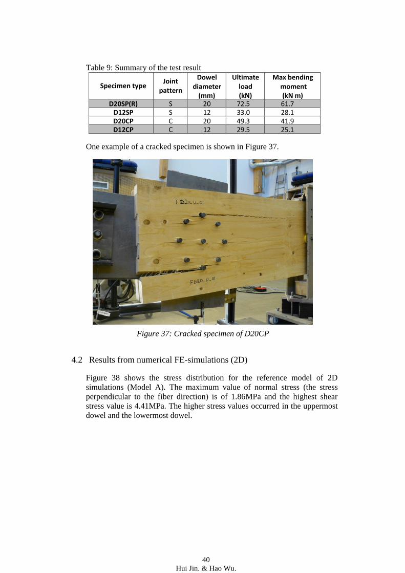
One example of a cracked specimen is shown in Figure 37.
Figure 37: Cracked specimen of D20CP
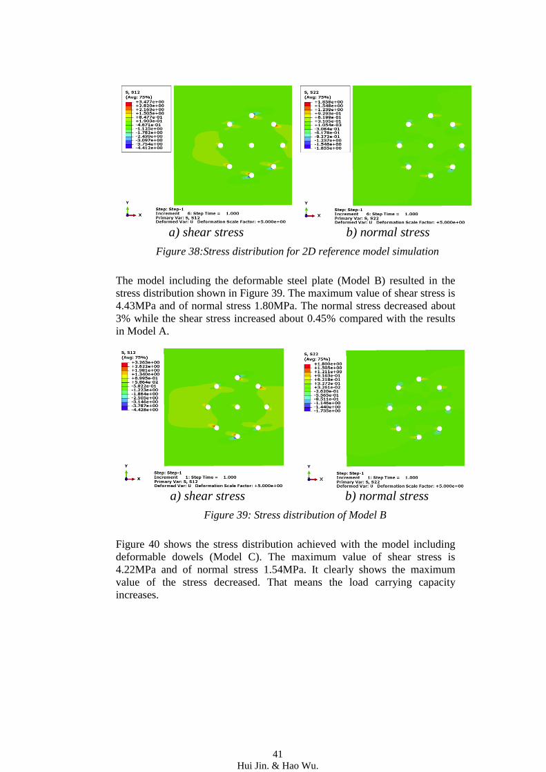
4.2 Results from numerical FE-simulations (2D)
Figure 38 shows the stress distribution for the reference model of 2D
simulations (Model A). The maximum value of normal stress (the stress
perpendicular to the fiber direction) is of 1.86MPa and the highest shear
stress value is 4.41MPa. The higher stress values occurred in the uppermost
dowel and the lowermost dowel.
41
Hui Jin. & Hao Wu.
a) shear stress b) normal stress
Figure 38:Stress distribution for 2D reference model simulation
The model including the deformable steel plate (Model B) resulted in the
stress distribution shown in Figure 39. The maximum value of shear stress is
4.43MPa and of normal stress 1.80MPa. The normal stress decreased about
3% while the shear stress increased about 0.45% compared with the results
in Model A.
a) shear stress b) normal stress
Figure 39: Stress distribution of Model B
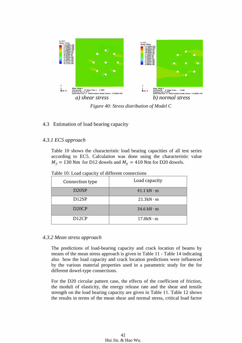
Figure 40 shows the stress distribution achieved with the model including
deformable dowels (Model C). The maximum value of shear stress is
4.22MPa and of normal stress 1.54MPa. It clearly shows the maximum
value of the stress decreased. That means the load carrying capacity
increases.
42
Hui Jin. & Hao Wu.
a) shear stress b) normal stress
Figure 40: Stress distribution of Model C
4.3 Estimation of load bearing capacity
4.3.1 EC5 approach
Table 10 shows the characteristic load bearing capacities of all test series
according to EC5. Calculation was done using the characteristic value
for D12 dowels and for D20 dowels.
Table 10: Load capacity of different connections
Connection type Load capacity
D20SP
D12SP
D20CP
D12CP
4.3.2 Mean stress approach
The predictions of load-bearing capacity and crack location of beams by
means of the mean stress approach is given in Table 11 - Table 14 indicating
also how the load capacity and crack location predictions were influenced
by the various material properties used in a parametric study for the for
different dowel-type connections.
For the D20 circular pattern case, the effects of the coefficient of friction,
the moduli of elasticity, the energy release rate and the shear and tensile
strength on the load bearing capacity are given in Table 11. Table 12 shows
the results in terms of the mean shear and normal stress, critical load factor
43
Hui Jin. & Hao Wu.
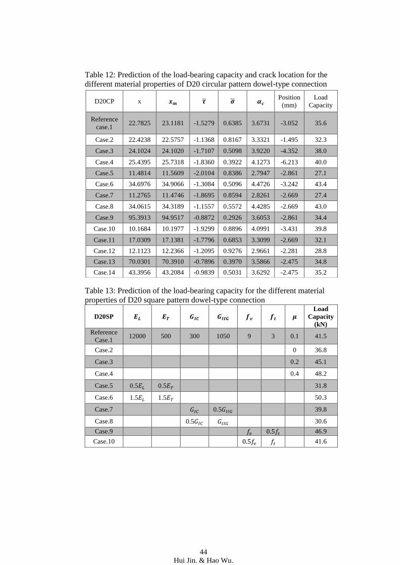
and crack location for the different cases. The corresponding results for the
D20 square pattern case are shown in Table13 and Table 14.
Note: for the variable friction coefficient and moduli of elasticity in D20SP,
CP cases, additional simulations with Abaqus were done. For other types of
variations only new post-processing of the results from the reference model
had to be done.
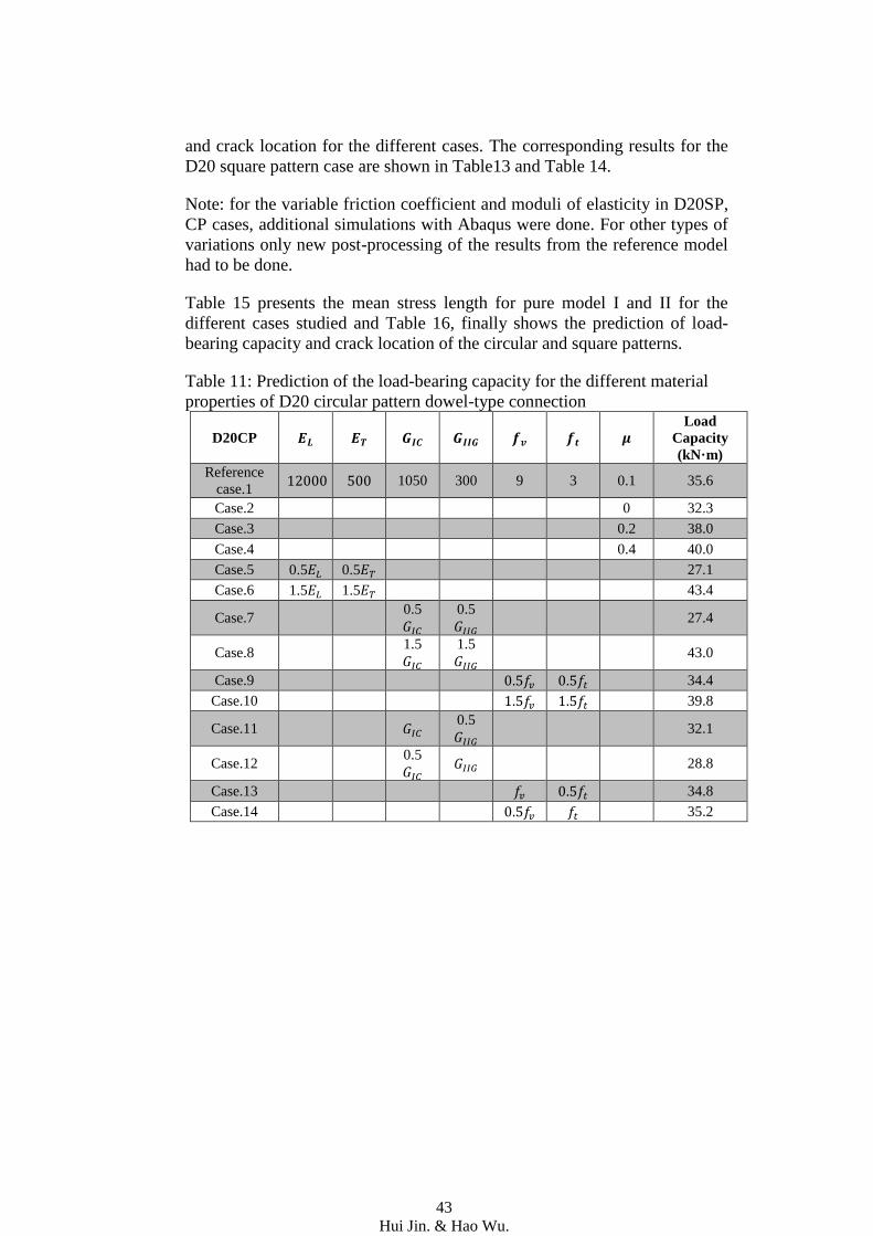
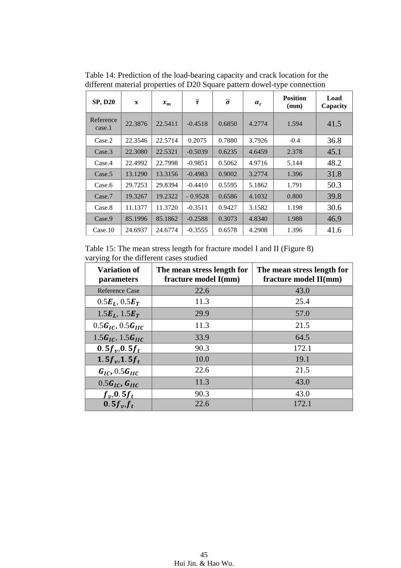
Table 15 presents the mean stress length for pure model I and II for the
different cases studied and Table 16, finally shows the prediction of load-
bearing capacity and crack location of the circular and square patterns.
Table 11: Prediction of the load-bearing capacity for the different material
properties of D20 circular pattern dowel-type connection
D20CP
Load
Capacity
(kN·m)
Reference
case.1 1050 300 9 3 0.1 35.6
Case.2 0 32.3
Case.3 0.2 38.0
Case.4 0.4 40.0
Case.5 0.5 0.5 27.1
Case.6 1.5 1.5 43.4
Case.7 0.5
0.5
27.4
Case.8 1.5
1.5
43.0
Case.9 34.4
Case.10 39.8
Case.11 0.5
32.1
Case.12 0.5
28.8
Case.13 34.8
Case.14 35.2
44
Hui Jin. & Hao Wu.
Table 12: Prediction of the load-bearing capacity and crack location for the
different material properties of D20 circular pattern dowel-type connection
Table 13: Prediction of the load-bearing capacity for the different material
properties of D20 square pattern dowel-type connection
D20SP
Load
Capacity
(kN)
Reference
Case.1 12000 500 300 1050 9 3 0.1 41.5
Case.2 0 36.8
Case.3 0.2 45.1
Case.4 0.4 48.2
Case.5 0.5 0.5 31.8
Case.6 1.5 1.5 50.3
Case.7 0.5 39.8
Case.8 0.5 30.6
Case.9 46.9
Case.10 41.6
D20CP x Position
(mm)
Load
Capacity
Reference
case.1 22.7825 23.1181 -1.5279 0.6385 3.6731 -3.052 35.6
Case.2 22.4238 22.5757 -1.1368 0.8167 3.3321 -1.495 32.3
Case.3 24.1024 24.1020 -1.7107 0.5098 3.9220 -4.352 38.0
Case.4 25.4395 25.7318 -1.8360 0.3922 4.1273 -6.213 40.0
Case.5 11.4814 11.5609 -2.0104 0.8386 2.7947 -2.861 27.1
Case.6 34.6976 34.9066 -1.3084 0.5096 4.4726 -3.242 43.4
Case.7 11.2765 11.4746 -1.8695 0.8594 2.8261 -2.669 27.4
Case.8 34.0615 34.3189 -1.1557 0.5572 4.4285 -2.669 43.0
Case.9 95.3913 94.9517 -0.8872 0.2926 3.6053 -2.861 34.4
Case.10 10.1684 10.1977 -1.9299 0.8896 4.0991 -3.431 39.8
Case.11 17.0309 17.1381 -1.7796 0.6853 3.3099 -2.669 32.1
Case.12 12.1123 12.2366 -1.2095 0.9276 2.9661 -2.281 28.8
Case.13 70.0301 70.3910 -0.7896 0.3970 3.5866 -2.475 34.8
Case.14 43.3956 43.2084 -0.9839 0.5031 3.6292 -2.475 35.2
45
Hui Jin. & Hao Wu.
Table 14: Prediction of the load-bearing capacity and crack location for the
different material properties of D20 Square pattern dowel-type connection
Table 15: The mean stress length for fracture model I and II (Figure 8)
varying for the different cases studied
Variation of
parameters
The mean stress length for
fracture model I(mm)
The mean stress length for
fracture model II(mm)
Reference Case 22.6 43.0
0.5 , 0.5 11.3 25.4
1.5 , 1.5 29.9 57.0
0.5 , 0.5 11.3 21.5
1.5 , 1.5 33.9 64.5
, 90.3 172.1
, 10.0 19.1
, 0.5 22.6 21.5
0.5 , 11.3 43.0
, 90.3 43.0
, 22.6 172.1
SP, D20 x Position
(mm)
Load
Capacity
Reference
case.1 22.3876 22.5411 -0.4518 0.6850 4.2774 1.594 41.5
Case.2 22.3546 22.5714 0.2075 0.7880 3.7926 -0.4 36.8
Case.3 22.3080 22.5321 -0.5039 0.6235 4.6459 2.378 45.1
Case.4 22.4992 22.7998 -0.9851 0.5062 4.9716 5.144 48.2
Case.5 13.1290 13.3156 -0.4983 0.9002 3.2774 1.396 31.8
Case.6 29.7253 29.8394 -0.4410 0.5595 5.1862 1.791 50.3
Case.7 19.3267 19.2322 - 0.9528 0.6586 4.1032 0.800 39.8
Case.8 11.1377 11.3720 -0.3511 0.9427 3.1582 1.198 30.6
Case.9 85.1996 85.1862 -0.2588 0.3073 4.8340 1.988 46.9
Case.10 24.6937 24.6774 -0.3555 0.6578 4.2908 1.396 41.6
46
Hui Jin. & Hao Wu.
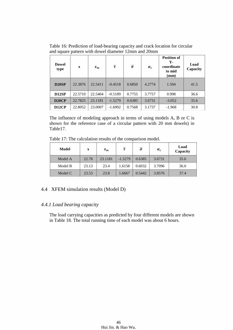
Table 16: Prediction of load-bearing capacity and crack location for circular
and square pattern with dowel diameter 12mm and 20mm
The influence of modeling approach in terms of using models A, B or C is
shown for the reference case of a circular pattern with 20 mm dowels) in
Table17.
Table 17: The calculation results of the comparison model.
4.4 XFEM simulation results (Model D)
4.4.1 Load bearing capacity
The load carrying capacities as predicted by four different models are shown
in Table 18. The total running time of each model was about 6 hours.
Dowel
type x
Position of
Y-
coordinate
to mid
(mm)
Load
Capacity
D20SP 22.3876 22.5411 -0.4518 0.6850 4.2774 1.594 41.5
D12SP 22.5710 22.5404 -0.5189 0.7755 3.7757 0.998 36.6
D20CP 22.7825 23.1181 -1.5279 0.6385 3.6731 -3.052 35.6
D12CP 22.8052 23.0007 -1.6992 0.7568 3.1737 -1.968 30.8
Model x Load
Capacity
Model A 22.78 23.1181 -1.5279 0.6385 3.6731 35.6
Model B 23.13 23.4 1.6158 0.6032 3.7096 36.0
Model C 23.53 23.8 1.6667 0.5442 3.8576 37.4
47
Hui Jin. & Hao Wu.
Table 18: The results of different XFEM modal simulations
XFEM
Model
Dowels
pattern
Amount of
initial crack
Timber
Elements
type
Rotation
displacement
[rad]
Load
Capacity
[kN·m]
1 D20SP 1 CPS4R 0.015 67.3
2 D20SP 2 CPS4R 0.015 57.2
3 D20CP 1 CPS4R 0.015 47.8
4 D20CP 2 CPS4R 0.015 43.5
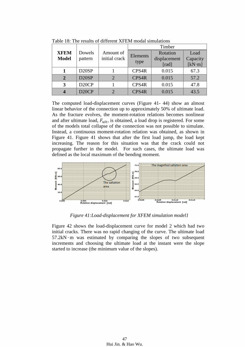
The computed load-displacement curves (Figure 41- 44) show an almost
linear behavior of the connection up to approximately 50% of ultimate load.
As the fracture evolves, the moment-rotation relations becomes nonlinear
and after ultimate load, , is obtained, a load drop is registered. For some
of the models total collapse of the connection was not possible to simulate.
Instead, a continuous moment-rotation relation was obtained, as shown in
Figure 41. Figure 41 shows that after the first load jump, the load kept
increasing. The reason for this situation was that the crack could not
propagate further in the model. For such cases, the ultimate load was
defined as the local maximum of the bending moment.
Figure 41:Load-displacement for XFEM simulation model1
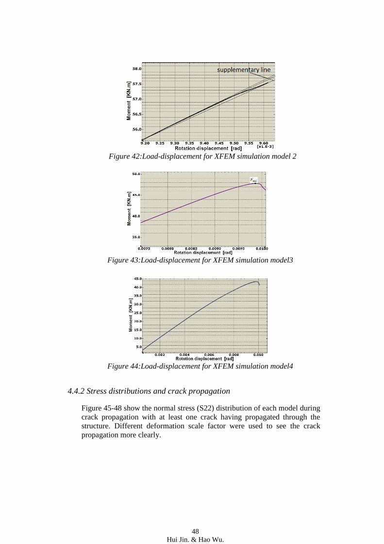
Figure 42 shows the load-displacement curve for model 2 which had two
initial cracks. There was no rapid changing of the curve. The ultimate load
57.2kN m was estimated by comparing the slopes of two subsequent
increments and choosing the ultimate load at the instant were the slope
started to increase (the minimum value of the slopes).
48
Hui Jin. & Hao Wu.
Figure 42:Load-displacement for XFEM simulation model 2
Figure 43:Load-displacement for XFEM simulation model3
Figure 44:Load-displacement for XFEM simulation model4
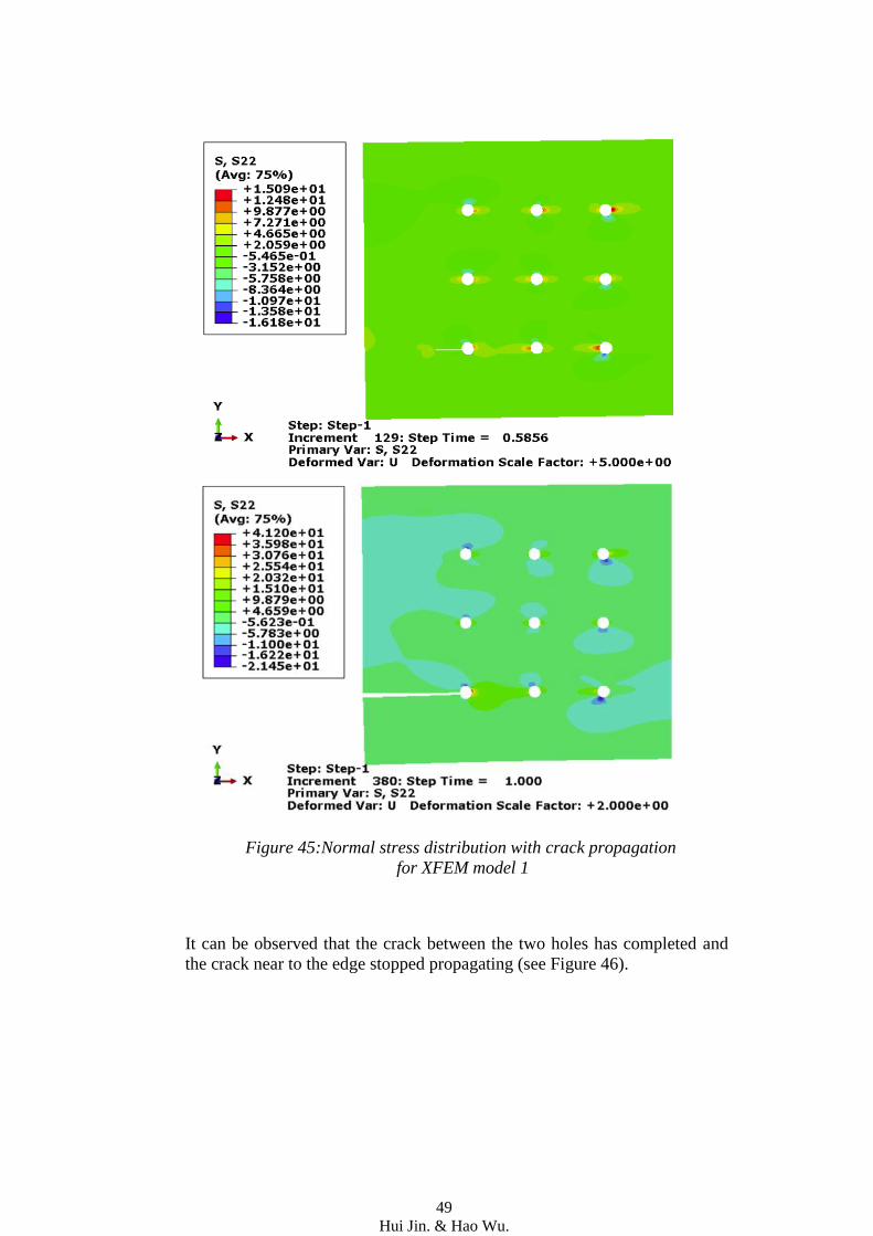
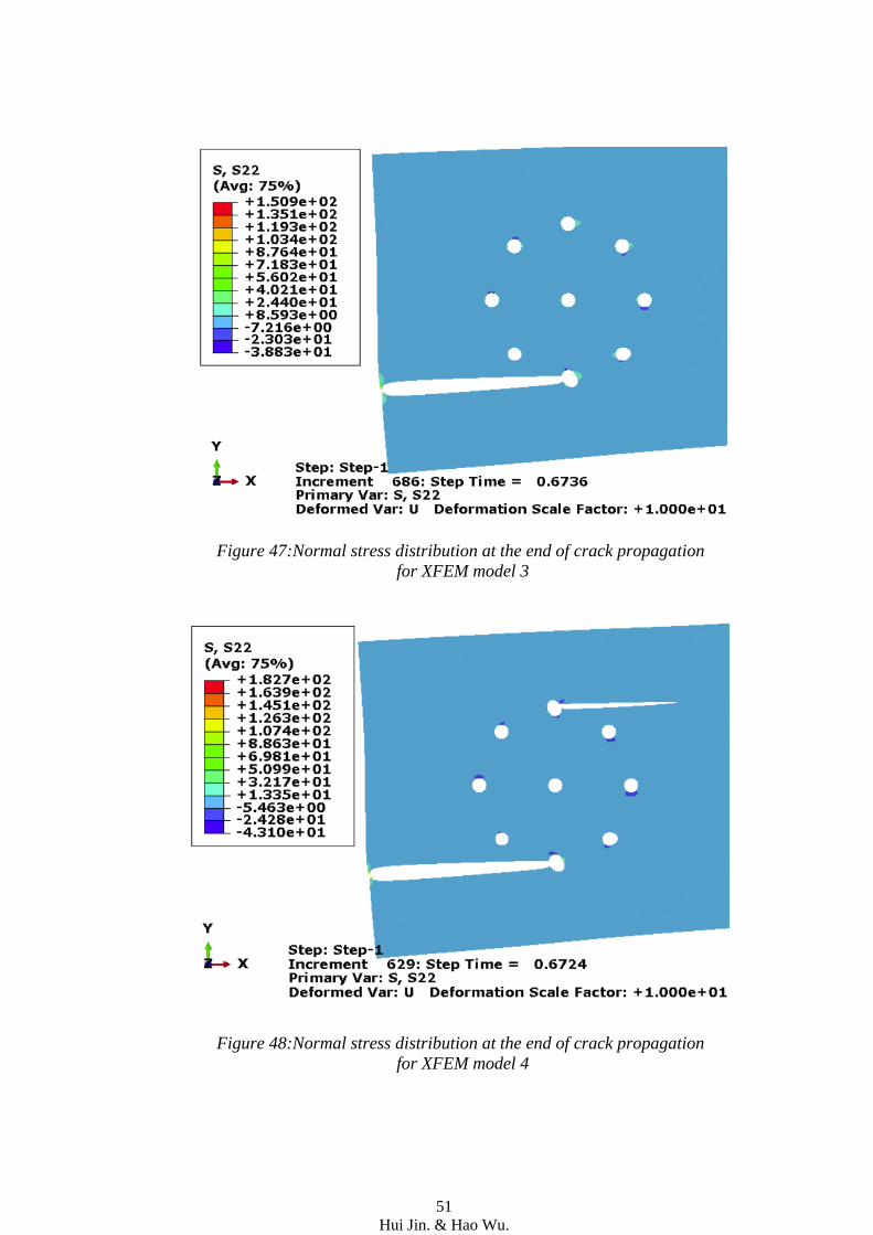
4.4.2 Stress distributions and crack propagation
Figure 45-48 show the normal stress (S22) distribution of each model during
crack propagation with at least one crack having propagated through the
structure. Different deformation scale factor were used to see the crack
propagation more clearly.
49
Hui Jin. & Hao Wu.
Figure 45:Normal stress distribution with crack propagation
for XFEM model 1
It can be observed that the crack between the two holes has completed and
the crack near to the edge stopped propagating (see Figure 46).

50
Hui Jin. & Hao Wu.
Figure 46:Normal stress distribution within crack propagation
for XFEM model 2
Figure 47 and 48 shows that there were still stresses in the vicinity of the left
edge of the crack surfaces. The reason is that although the crack surfaces
separated, the last pair of nodes would not separate.
51
Hui Jin. & Hao Wu.
Figure 47:Normal stress distribution at the end of crack propagation
for XFEM model 3
Figure 48:Normal stress distribution at the end of crack propagation
for XFEM model 4
52
Hui Jin. & Hao Wu.
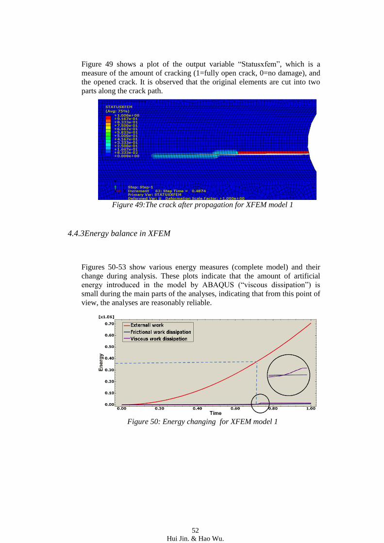
Figure 49 shows a plot of the output variable “Statusxfem”, which is a
measure of the amount of cracking (1=fully open crack, 0=no damage), and
the opened crack. It is observed that the original elements are cut into two
parts along the crack path.
Figure 49:The crack after propagation for XFEM model 1
4.4.3Energy balance in XFEM
Figures 50-53 show various energy measures (complete model) and their
change during analysis. These plots indicate that the amount of artificial
energy introduced in the model by ABAQUS (“viscous dissipation”) is
small during the main parts of the analyses, indicating that from this point of
view, the analyses are reasonably reliable.
Figure 50: Energy changing for XFEM model 1

53
Hui Jin. & Hao Wu.
Figure 51 Energy changing for XFEM model 2
Figure 52:Energy changing for XFEM model 3
Figure 53: Energy changing for XFEM model 4
4.5 3D simulation results (Model E)
The results of 3D simulation focused on the deformation patterns and stress
distributions, especially the normal stress distribution in different cases. The
3D simulation model 3, which used the quadratic geometric order elements,
54
Hui Jin. & Hao Wu.
is believed to give the most accurate stress distribution, but its computing
time was nearly 3 days.
4.5.1 Stress distribution for different models
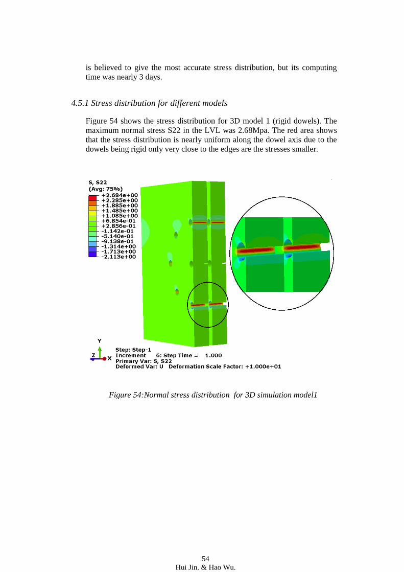
Figure 54 shows the stress distribution for 3D model 1 (rigid dowels). The
maximum normal stress S22 in the LVL was 2.68Mpa. The red area shows
that the stress distribution is nearly uniform along the dowel axis due to the
dowels being rigid only very close to the edges are the stresses smaller.
Figure 54:Normal stress distribution for 3D simulation model1
55
Hui Jin. & Hao Wu.
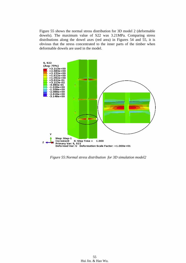
Figure 55 shows the normal stress distribution for 3D model 2 (deformable
dowels). The maximum value of S22 was 3.21MPa. Comparing stress
distributions along the dowel axes (red area) in Figures 54 and 55, it is
obvious that the stress concentrated to the inner parts of the timber when
deformable dowels are used in the model.
Figure 55:Normal stress distribution for 3D simulation model2
56
Hui Jin. & Hao Wu.
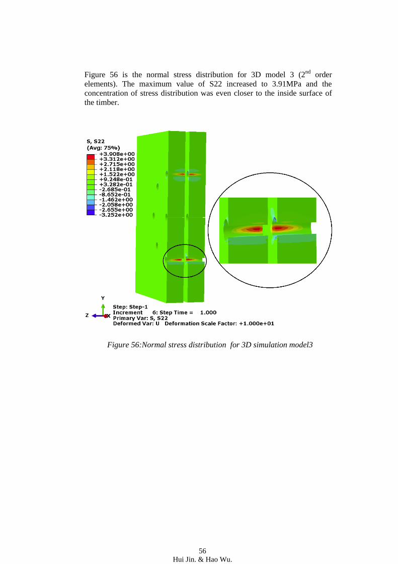
Figure 56 is the normal stress distribution for 3D model 3 (2nd
order
elements). The maximum value of S22 increased to 3.91MPa and the
concentration of stress distribution was even closer to the inside surface of
the timber.
Figure 56:Normal stress distribution for 3D simulation model3
57
Hui Jin. & Hao Wu.
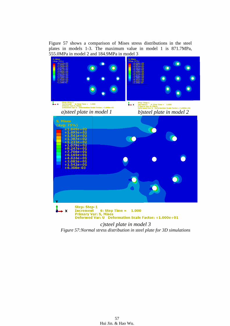
Figure 57 shows a comparison of Mises stress distributions in the steel
plates in models 1-3. The maximum value in model 1 is 871.7MPa,
555.0MPa in model 2 and 184.9MPa in model 3
a)steel plate in model 1 b)steel plate in model 2
c)steel plate in model 3
Figure 57:Normal stress distribution in steel plate for 3D simulations
58
Hui Jin. & Hao Wu.
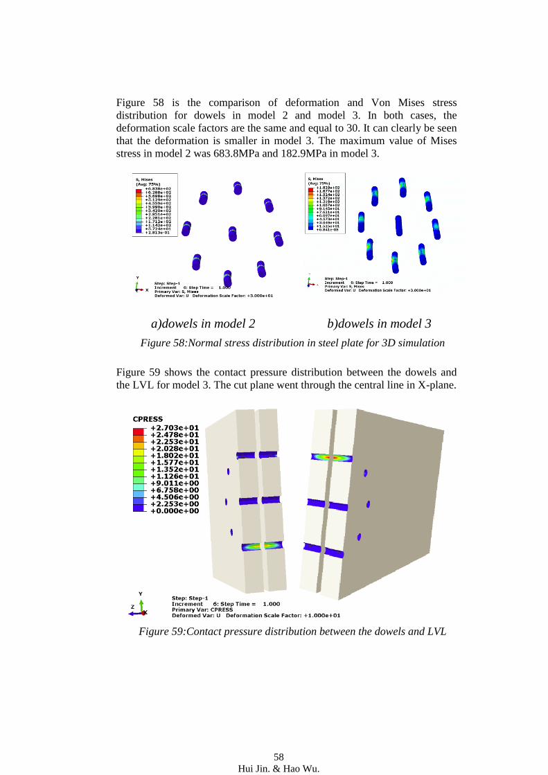
Figure 58 is the comparison of deformation and Von Mises stress
distribution for dowels in model 2 and model 3. In both cases, the
deformation scale factors are the same and equal to 30. It can clearly be seen
that the deformation is smaller in model 3. The maximum value of Mises
stress in model 2 was 683.8MPa and 182.9MPa in model 3.
a)dowels in model 2 b)dowels in model 3
Figure 58:Normal stress distribution in steel plate for 3D simulation
Figure 59 shows the contact pressure distribution between the dowels and
the LVL for model 3. The cut plane went through the central line in X-plane.
Figure 59:Contact pressure distribution between the dowels and LVL
59
Hui Jin. & Hao Wu.
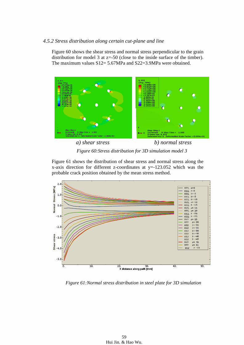
4.5.2 Stress distribution along certain cut-plane and line
Figure 60 shows the shear stress and normal stress perpendicular to the grain
distribution for model 3 at z=-50 (close to the inside surface of the timber).
The maximum values S12= 5.67MPa and S22=3.9MPa were obtained.
a) shear stress b) normal stress
Figure 60:Stress distribution for 3D simulation model 3
Figure 61 shows the distribution of shear stress and normal stress along the
x-axis direction for different z-coordinates at y=-123.052 which was the
probable crack position obtained by the mean stress method.
Figure 61:Normal stress distribution in steel plate for 3D simulation
60
Hui Jin. & Hao Wu.
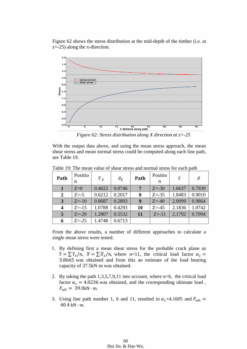
Figure 62 shows the stress distribution at the mid-depth of the timber (i.e. at
z=-25) along the x-direction.
Figure 62: Stress distribution along X direction at z=-25
With the output data above, and using the mean stress approach, the mean
shear stress and mean normal stress could be computed along each line path,
see Table 19.
Table 19: The mean value of shear stress and normal stress for each path
Path Position
Path Positio
n
1 Z=0 0.4022 0.0746 7 Z=-30 1.6637 0.7939
2 Z=-5 0.6212 0.2017 8 Z=-35 1.8483 0.9010
3 Z=-10 0.8687 0.2893 9 Z=-40 2.0099 0.9864
4 Z=-15 1.0788 0.4293 10 Z=-45 2.1836 1.0742
5 Z=-20 1.2807 0.5532 11 Z=-51 2.1792 0.7094
6 Z=-25 1.4748 0.6713
From the above results, a number of different approaches to calculate a
single mean stress were tested.
1. By defining first a mean shear stress for the probable crack plane as
∑ ∑ where n=11, the critical load factor was obtained and from this an estimate of the load bearing
capacity of 37.5kN·m was obtained.
2. By taking the path 1,3,5,7,9,11 into account, where n=6, the critical load
factor was obtained, and the corresponding ultimate load ,
3. Using line path number 1, 6 and 11, resulted in =4.1605 and
61
Hui Jin. & Hao Wu.
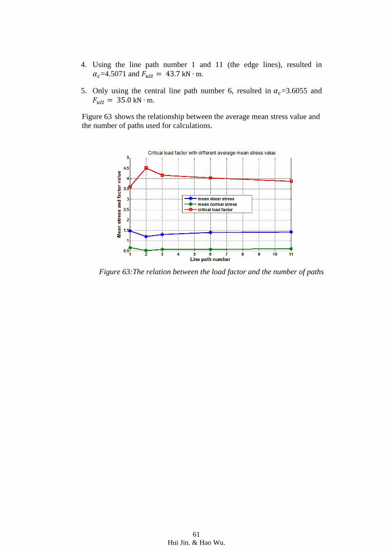
4. Using the line path number 1 and 11 (the edge lines), resulted in
=4.5071 and
5. Only using the central line path number 6, resulted in =3.6055 and
Figure 63 shows the relationship between the average mean stress value and
the number of paths used for calculations.
Figure 63:The relation between the load factor and the number of paths
62
Hui Jin. & Hao Wu.
5. Analysis and discussion
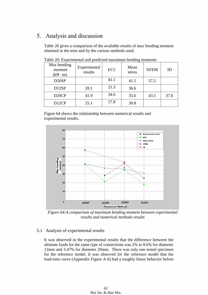
Table 20 gives a comparison of the available results of max bending moment
obtained in the tests and by the various methods used.
Table 20: Experimental and predicted maximum bending moments
Max bending moment
(k )
Experimental
results EC5
Mean
stress XFEM 3D
D20SP 41.1 41.5 57.2
D12SP 28.1 21.3 36.6
D20CP 41.9 34.6 35.6 43.5 37.6
D12CP 25.1 17.8 30.8
Figure 64 shows the relationship between numerical results and
experimental results.
Figure 64:A comparison of maximum bending moment between experimental
results and numerical methods results
5.1 Analysis of experimental results
It was observed in the experimental results that the difference between the
ultimate loads for the same type of connections was 2% to 8.6% for diameter
12mm and 3.47% for diameter 20mm. There was only one tested specimen
for the reference model. It was observed for the reference model that the
load-time curve (Appendix Figure A-6) had a roughly linear behavior before

63
Hui Jin. & Hao Wu.
the ultimate load was reached. For the specimens of diameter 12mm, the
dowel had reached the plastic deformation during the test before the timber
cracks occurred (Appendix Figure A-4).
5.2 Analysis of EC5 results and discussion
It is obvious that the predictions obtained by the EC5 approach are much
smaller than the experimental results (see Table 10). This is reasonable,
since the characteristic embedding strength was used for the calculation.
This means, in principle that 95% of the test results will show a higher load
bearing capacity than the computed results using the EC5 approach.
The numerical results obtained with the EC5-appraoch of type D12CP is
40% smaller compared with the experimental result. For the D20CP
specimens the predictions is 17% smaller than the experimental result. The
reason for this difference could be that the dowel of diameter 12mm yielded
(large deformation) before the timber structure failed (see Appendix Figure
A-4 and A-4), and this is not correctly accounted for in the EC5-approach.
Since a limited number of specimens were tested, the influence of different
dowel patterns cannot be clearly observed. However, the EC5-approach
seems to give the same trend as the tests: for the dowels used here, the
square pattern gives a slightly higher load bearing capacity.
5.3 Analysis and discussion of mean stress results
From Table 6, there is a difference less than 1% between the critical load
factors for the three most critical crack paths.
To obtain accurate results and comprehend how the parameters influence the
structures, 14 configurations of D20 circular pattern and 10 configurations
of D20 square pattern were analyzed with the mean stress approach; the
results are available in Table 11 and Table 14.
It is obvious in Table 11 case 1-4 (D20CP), that the load-bearing capacity
increased approximate linearly with the coefficient of friction. What is more,
the crack location (Table 12 case 1-4) moves from the center of the dowel
(i.e. in the y-direction) when the coefficient of friction increases. The same
tendency is seen for the D20SP case and shown in Table 14 case 1-4.
Obviously, for the variations of the moduli of elasticity (Table 12
cases 5-6), it can be considered that the load-bearing capacity increased with
increasing moduli of elasticity. An increased modulus of elasticity increases
the means stress length, and thus reduces the mean stress used in the
evaluation. In addition, the calculation results show that the crack location
will not move as the elasticity moduli are changed (this because all moduli
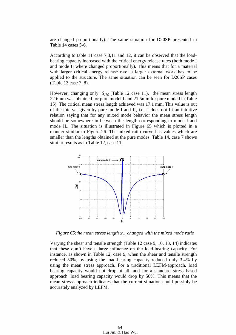
64
Hui Jin. & Hao Wu.
are changed proportionally). The same situation for D20SP presented in
Table 14 cases 5-6.
According to table 11 case 7,8,11 and 12, it can be observed that the load-
bearing capacity increased with the critical energy release rates (both mode I
and mode II where changed proportionally). This means that for a material
with larger critical energy release rate, a larger external work has to be
applied to the structure. The same situation can be seen for D20SP cases
(Table 13 case 7, 8).
However, changing only (Table 12 case 11), the mean stress length
22.6mm was obtained for pure model I and 21.5mm for pure mode II (Table
15). The critical mean stress length achieved was 17.1 mm. This value is out
of the interval given by pure mode I and II, i.e. it does not fit an intuitive
relation saying that for any mixed mode behavior the mean stress length
should be somewhere in between the length corresponding to mode I and
mode II.. The situation is illustrated in Figure 65 which is plotted in a
manner similar to Figure 26. The mixed ratio curve has values which are
smaller than the lengths obtained at the pure modes. Table 14, case 7 shows
similar results as in Table 12, case 11.
Figure 65:the mean stress length changed with the mixed mode ratio
Varying the shear and tensile strength (Table 12 case 9, 10, 13, 14) indicates
that these don’t have a large influence on the load-bearing capacity. For
instance, as shown in Table 12, case 9, when the shear and tensile strength
reduced 50%, by using the load-bearing capacity reduced only 3.4% by
using the mean stress approach. For a traditional LEFM-approach, load
bearing capacity would not drop at all, and for a standard stress based
approach, load bearing capacity would drop by 50%. This means that the
mean stress approach indicates that the current situation could possibly be
accurately analyzed by LEFM.
65
Hui Jin. & Hao Wu.
However, as shown in Table 15, changing only the tensile strength, the mean
stress length for pure mode I is 90.3mm and for pure model II is 43mm. The
achieved critical mean stress length was 85mm as shown in Table 14 case 9.
In this case, the mean shear stress influence increased and the mean normal
stress influence increased (i.e. k increased) and, thus, the load-bearing
capacity (46.9kN·m) is 11.5% higher than the D20SP reference case
(41.5kN·m).
The cases involving large changes of one strength parameter only are
believed not to be realistic since, in general one would expect some
correlation between elastic moduli, strength and fracture energies.
5.4 Analysis and discussion of results for XFEM simulation
The main results computed with XFEM simulation was presented in Table
18. The prediction for XFEM model 4 was 43.5kN m when two initial
cracks were predefined. This result had an error of +3.82% compared with
the experimental result. However, only one specimen of a type similar to the
reference model has been tested, so the accuracy of the predictions is
unclear.
As shown in Table 18, the predicted ultimate load with one initial crack was
larger than which has two initial cracks. This comparison fits the assumption
of the fracture mechanical theory: Less strength will be obtained if it has
more flaws. Thus the assumption of linear elastic material is used, the non-
linear behavior occurred due to the non-linear geometry within the crack
propagation.
According to the configuration of the crack propagation (Figure 45-48), all
cracks propagated along the fiber direction of the timber. It’s reasonable for
the material property of orthotropic elasticity and it was confirmed by the
experiment as well. The shear displacement (the slight sliding along x-
direction between the crack surfaces) can be observed as well. This fracture
behavior confirms that the model was subjected to a mixed fracture mode
containing both mode I and mode II (Figure 8).
The energy curves (Figures 50-53) show how the external work, the
frictional dissipation and the viscous dissipation change during the crack
propagation. It is observed that the total external work for XFEM model 1
(Figure 50) is larger than for XFEM model 2. This is in line with the result
in terms of ultimate load. It can be observed that the frictional dissipation in
these figures is zero. That means the displacements along the frictional load
direction are zero. The viscous dissipation of the models is at very low
values until the ultimate load occurs. This means that the artificial damping
introduced by the FE-software does not play an important role.
66
Hui Jin. & Hao Wu.
The XFEM simulations gave results which coincided well with the
experimental findings. The effects of different parameters has not been
considered in this thesis, additional studies would be needed.
5.5 Analysis and discussion of 3D simulation
It is assumed in general that the stress distributions obtained for the model
which used the quadratic elements (Figure 54-56) are the most accurate. The
concentration of stress was much closer to the inside surface of the timber
comparing model 3 to model 1.
For Figure 58 a), the maximum value of Von Mises stress had reached
683.8MPa which is above the yield strength of the dowels. Figure 59 shows
the contact pressure between the dowels and the timber. It is observed that
there was no contact pressure in the central dowel which is also predicted by
the EC5-approach. The lower and upper dowels act similar and the small
difference between the upper and lower dowels is due to the fact that the
lower dowels are closer to the edge.
Figure 60 shows a very similar appearance compared to the 2D numerical
model (Figure 38) but the maximum value of stress varies. According to
Figure 61, the stress levels increased from the outside surface to the inside
surface. The stress distribution is reasonable because the deformation of the
timber near the vicinity of dowel was caused by the dowels and it increased
from the outside to inside due to the geometry.
By using the average value of the mean stress in Table 19, the ultimate load
37.5 was achieved and this value differs by 5% compared with the
reference model. The difference was 0.2% compared with the 2D model
which had the deformable dowels (Table 17). It shows the consistency
between the 2D and 3D models.
Figure 63 shows how the critical load factor and the average of mean stress
varied with the numbers of line paths used in an attempt to extend the
normally 2D-mean stress method into 3D. This approach seems to be one
way to make such an extension, and it is recommended to use values from
the paths at the edges plus at least one central path.
67
Hui, Jin. & Hao, Wu.
6. Conclusions and future work
Four numerical approaches were adopted in this project in order to predict
the load carrying capacity of multiple dowel-type steel to timber
connections. The numerical methods could predict the influence of the
different dowel patterns. Some of the numerical results are quite close to the
experiments. However, most of the values of material properties were taken
from other literature and not from measurements, and here, additional
studies are needed.
The advantage of the EC5-approach is that this method is simple use in
hand-calculations to obtain the load distribution for each single dowel and to
evaluate the load capacity.
The mean stress approach has good correlation to experiments. This method
has the advantage that it makes possible to study the influence of the elastic
material properties and the fracture properties. For instance, the load
carrying capacity increased with increasing friction as reported in previous
literature.
The XFEM results had the lowest error of +3.82% compared with the
experimental results and it can describe the crack propagation at the same
time. The initial crack location can be obtained using a simple assumption of
a straight line starting from a point determined by the mean stress method as
mentioned in section 3.3.2. It also can be used to simulate more complex
crack situations, which would be of interest for future studies.
The 3D model shows a very similar stress distribution as compared to the
2D model. It is useful for illustrating the general deformation behavior and
the stress distribution through arbitrary sections of the structure. To ensure
the accuracy of the 3D simulation results and to create a model with fewer
elements, elements of quadratic geometric order is recommended. An
interesting observation is the extended mean stress method for 3D
simulation proposed here, which gave a similar prediction of the load
bearing capacity as compared to the 2D simulations.
In general, the numerical methods used here, should be possible to apply for
other loading cases than pure bending, and also for other dowel
configurations. This would be a very interesting future research task. Since it
is difficult to find in literature results from such tests, also experimental
investigations would be of interest.
A
Hui, Jin. & Hao, Wu.
References
ABAQUS Inc. (2013). ABAQUS/Standard and ABAQUS/CAE Version
6.13-2, User Manuals.
Ad Leijten, Jochen Köhler, and André Jorissen (2004). Review of probability
data for timber connections with dowel-type fasteners. Timber structures, 2004;
37: 7-13.
Aicher S, Gustafsson PJ (ed), Haller P, Petersson H (2002). Fracture
mechanics models for strength analysis of timber beams with a hole or a
notch – a report of RILEM TC-133. Report TVSM-7134, Lund University,
Sweden
Anderson, T.L. (1994). Fracture Mechanics. Fundamentals and
Applications. CRC Press
Ardalany M, Deam B, Fragiacomo M (2010). Experimental results of
fracture energy and fracture toughness of Radiata Pine laminated veneer
lumber (LVL) in model I (opening). Materials and structures, 2012; 45:
1189-1205.
Belytschko, T., Black, T. (1999) Elastic crack growth in finite elements with
minimal remeshing. International Journal for Numerical Methods in
Engineering; 45:601–620.
Blyberg, L. (2008) Modelling the effect of cracks in an inverted double-
tapered glulam beam. Master thesis, Växjö University Eurocode 5 (2011)
Eurocode 5 - Design of Timber Structures. EN 1995-1-1:2011
Dolbow, J. (1999) an extended finite element method with discontinuous
enrichment for applied mechanics. PhD thesis, Northwestern University.
E. Giner, N. Sukumar, J.E. Tarancon, and F.J. Fuenmayor (2008). An
abaqus implementation of extended finite element method. Engineering
fracture mechanics, 2009; 76: 347-368.
Gdoutos, E.E. (1993) Fracture Mechanics. An introduction. Netherlands,
Kluwer Academic
Gustafsson, P. J. (2002) Mean stress approach and initial crack approach In:
Aicher S. Gustafsson, PJ (ed). Haller, P. and Petersson, H., Fracture
mechanics models for strength analysis of timber beams with a hole or a
notch - a report of RILEM TC-133. Report TVSM-7134, Lund University,
Sweden.
Handbok och formelsamling i Hållfasthetslära. (In Swedish) Department of
Solid Mechanics, Royal Institute of Technology (KTH), Stockholm, 1999
B
Hui, Jin. & Hao, Wu.
Henrik, Danielsson. (2007) the strength of glulam beams with holes. A
survey of tests and Calculation methods. KFS I Lund AB, Lund, Sweden,
2007
Irwin, G. (1957) Analysis of stresses and strains near the end of a crack
traversing a plane, Journal of Applied Mechanics 24,361-364
Johansen, K. (1949). Theory of Timber Connections In international
Association for bridge and structural Engineering (IABSE) Pub 9
Michael, Dorn. (2012). Investigations on the Serviceability Limit State of
Dowel-type Timber Connections. Doctoral thesis, Vienna University of
Technology.
Moes, N., Dolbow, J., Belytschko, T. (1999). A finite element method for
crack growth without remeshing. Int J Numer Meth Eng. 46:131–150
Niels Ottosen,Hans Petersson (1992). Introduction to the finite element
method. Prentice Hall, 1 edition, 1992.
Richardson, C.L., Hegemann, J., al.(2009) An XFEM method for modelling
geometrically elaborate crack propagation in brittle materials. International
Journal For Numerical Method in Engineering. Int. J. Meth. Engng.1:1
Serrano, Erik., Enquist, Bertil.(2013) MechWood II. Tests on dowel type
joints. Lineaus University.
Serrano, E. and Gustafsson, P.J. (2006) Fracture Mechanics in timber
engineering-Strength analyses of components and joints. RILEM 2006
Serrano, Erik, Gustafsson, P.J.(2006) Fracture mechanics in timber
engineering – Strength analyses of components and joints, Material and
structures 40: 87-96
Swedishwood (2014), Available at
http://www.swedishwood.com/facts_about_wood/wood_industry/swedish_s
awmills_in_brief [Accessed 2014.01.29]
Sjödin, Johan. (2008) Strength and moisture aspects of steel-timber dowel
joints in glulam structures – an Experimental and Numerical Study. Doctor
thesis, Växjö University
Sjödin, Johan., Serrano, Erik. (2008). A numerical study to predict the
capacity of multiply steel-timber dowel joints, Holz Roh Werkst 2008;
66:447-454.
Sjödin, Johan., Serrano, Erik., Bertil, Enquist. (2008). An experimental and
numerical study of effect of friction in single dowel joints, Holz Roh Werkst
2008; 66: 363-372
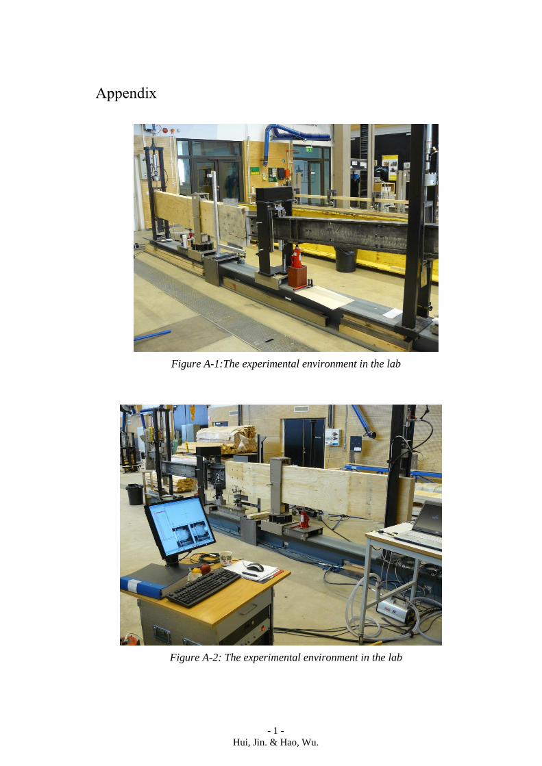
- 1 -
Hui, Jin. & Hao, Wu.
Appendix
Figure A-1:The experimental environment in the lab
Figure A-2: The experimental environment in the lab
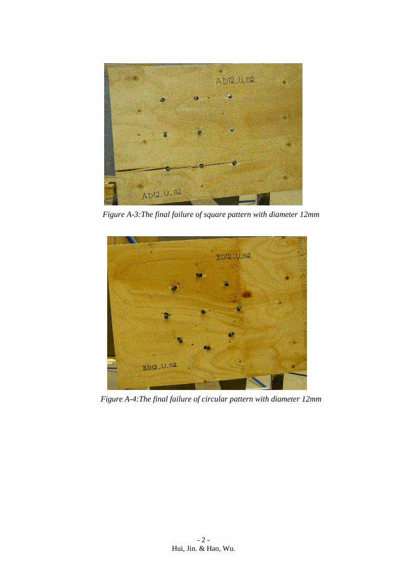
- 2 -
Hui, Jin. & Hao, Wu.
Figure A-3:The final failure of square pattern with diameter 12mm
Figure A-4:The final failure of circular pattern with diameter 12mm
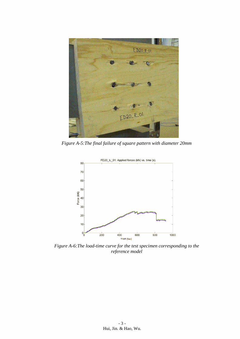
- 3 -
Hui, Jin. & Hao, Wu.
Figure A-5:The final failure of square pattern with diameter 20mm
Figure A-6:The load-time curve for the test specimen corresponding to the
reference model
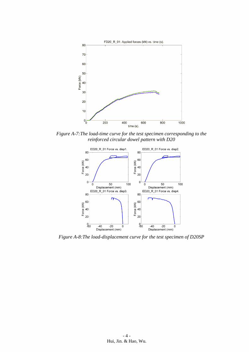
- 4 -
Hui, Jin. & Hao, Wu.
Figure A-7:The load-time curve for the test specimen corresponding to the
reinforced circular dowel pattern with D20
Figure A-8:The load-displacement curve for the test specimen of D20SP
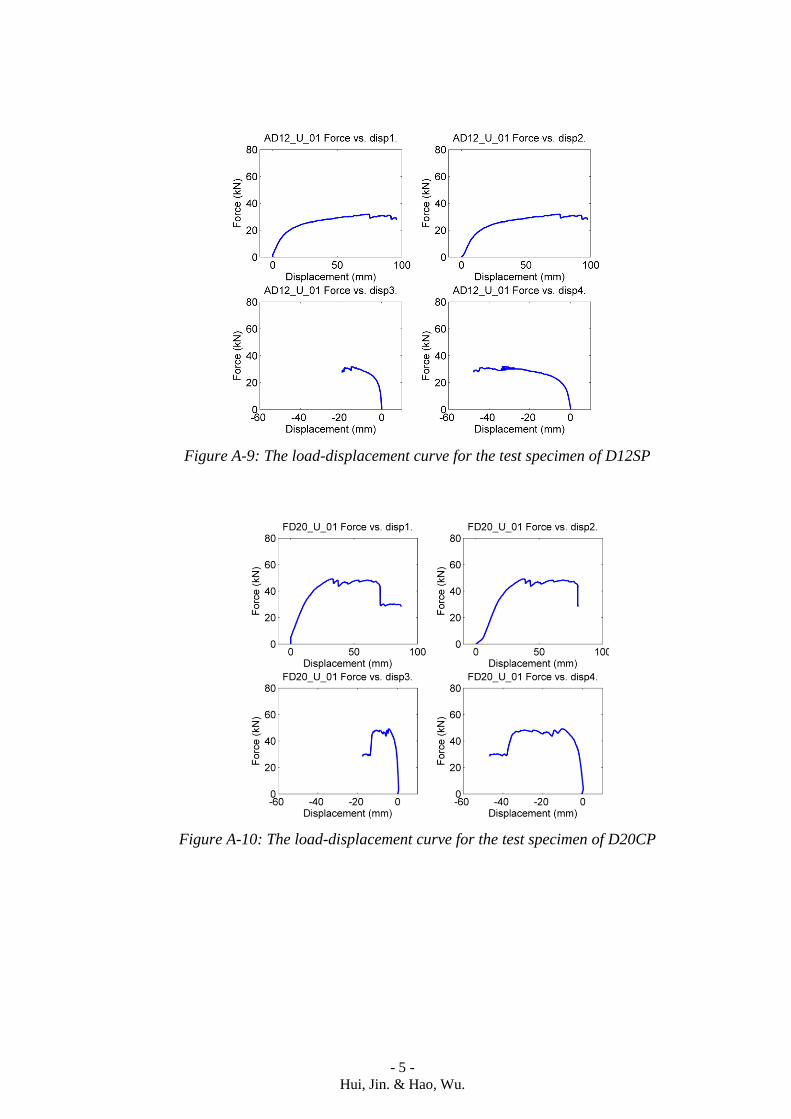
- 5 -
Hui, Jin. & Hao, Wu.
Figure A-9: The load-displacement curve for the test specimen of D12SP
Figure A-10: The load-displacement curve for the test specimen of D20CP
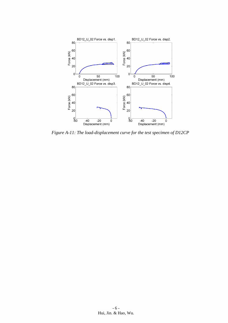
- 6 -
Hui, Jin. & Hao, Wu.
Figure A-11: The load-displacement curve for the test specimen of D12CP
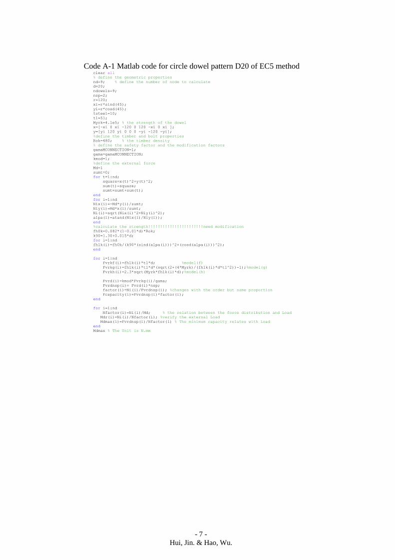
- 7 -
Hui, Jin. & Hao, Wu.
Code A-1 Matlab code for circle dowel pattern D20 of EC5 method clear all
% define the geometric properties
nd=9; % define the number of node to calculate
d=20;
ndowels=9;
nsp=2;
r=120;
xi=r*sind(45);
yi=r*cosd(45);
tsteel=10;
t1=51;
Myrk=4.1e5; % the strength of the dowel
x=[-xi 0 xi -120 0 120 -xi 0 xi ];
y=[yi 120 yi 0 0 0 -yi -120 -yi];
%define the timber and bolt properties
Rok=480; % the timber density
% define the safety factor and the modification factors
gamaMCONNECTION=1;
gama=gamaMCONNECTION;
kmod=1;
%define the external force
Md=1
sumt=0;
for t=1:nd;
square=x(t)^2+y(t)^2;
sum(t)=square;
sumt=sumt+sum(t);
end
for i=1:nd
Nix(i)=-Md*y(i)/sumt;
Niy(i)=Md*x(i)/sumt;
Ni(i)=sqrt(Nix(i)^2+Niy(i)^2);
alpa(i)=atand(Nix(i)/Niy(i));
end
%calculate the strength!!!!!!!!!!!!!!!!!!!!!!!need modification
fh0k=0.082*(1-0.01*d)*Rok;
k90=1.30+0.015*d;
for i=1:nd
fh1k(i)=fh0k/(k90*(sind(alpa(i)))^2+(cosd(alpa(i)))^2);
end
for i=1:nd
Fvrkf(i)=fh1k(i)*t1*d; %model(f)
Fvrkg(i)=fh1k(i)*t1*d*(sqrt(2+(4*Myrk)/(fh1k(i)*d*t1^2))-1);%model(g)
Fvrkh(i)=2.3*sqrt(Myrk*fh1k(i)*d);%model(h)
Fvrd(i)=kmod*Fvrkg(i)/gama;
Fvrdnsp(i)= Fvrd(i)*nsp;
factor(i)=Ni(i)/Fvrdnsp(i); %changes with the order but same proportion
Fcapacity(i)=Fvrdnsp(i)*factor(i);
end
for i=1:nd
Nfactor(i)=Ni(i)/Md; % the relation between the force distribution and Load
Mdr(i)=Ni(i)/Nfactor(i); %verify the external Load
Mdmax(i)=Fvrdnsp(i)/Nfactor(i) % The minimum capacity relates with Load
end
Mdmax % The Unit is N.mm
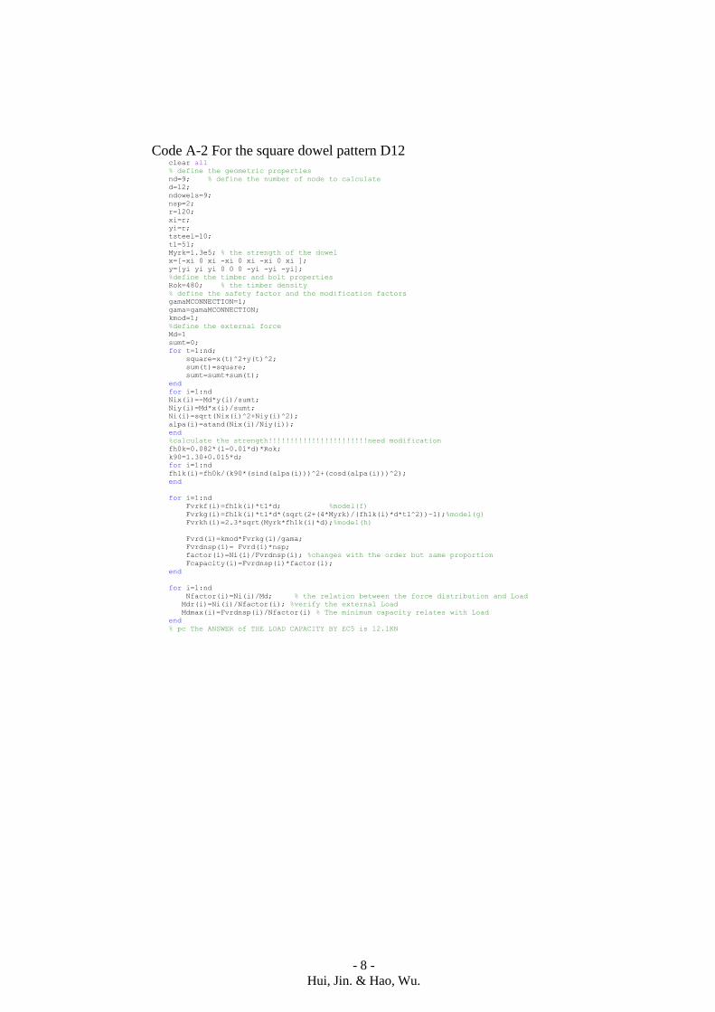
- 8 -
Hui, Jin. & Hao, Wu.
Code A-2 For the square dowel pattern D12 clear all
% define the geometric properties
nd=9; % define the number of node to calculate
d=12;
ndowels=9;
nsp=2;
r=120;
xi=r;
yi=r;
tsteel=10;
t1=51;
Myrk=1.3e5; % the strength of the dowel
x=[-xi 0 xi -xi 0 xi -xi 0 xi ];
y=[yi yi yi 0 0 0 -yi -yi -yi];
%define the timber and bolt properties
Rok=480; % the timber density
% define the safety factor and the modification factors
gamaMCONNECTION=1;
gama=gamaMCONNECTION;
kmod=1;
%define the external force
Md=1
sumt=0;
for t=1:nd;
square=x(t)^2+y(t)^2;
sum(t)=square;
sumt=sumt+sum(t);
end
for i=1:nd
Nix(i)=-Md*y(i)/sumt;
Niy(i)=Md*x(i)/sumt;
Ni(i)=sqrt(Nix(i)^2+Niy(i)^2);
alpa(i)=atand(Nix(i)/Niy(i));
end
%calculate the strength!!!!!!!!!!!!!!!!!!!!!!!need modification
fh0k=0.082*(1-0.01*d)*Rok;
k90=1.30+0.015*d;
for i=1:nd
fh1k(i)=fh0k/(k90*(sind(alpa(i)))^2+(cosd(alpa(i)))^2);
end
for i=1:nd
Fvrkf(i)=fh1k(i)*t1*d; %model(f)
Fvrkg(i)=fh1k(i)*t1*d*(sqrt(2+(4*Myrk)/(fh1k(i)*d*t1^2))-1);%model(g)
Fvrkh(i)=2.3*sqrt(Myrk*fh1k(i)*d);%model(h)
Fvrd(i)=kmod*Fvrkg(i)/gama;
Fvrdnsp(i)= Fvrd(i)*nsp;
factor(i)=Ni(i)/Fvrdnsp(i); %changes with the order but same proportion
Fcapacity(i)=Fvrdnsp(i)*factor(i);
end
for i=1:nd
Nfactor(i)=Ni(i)/Md; % the relation between the force distribution and Load
Mdr(i)=Ni(i)/Nfactor(i); %verify the external Load
Mdmax(i)=Fvrdnsp(i)/Nfactor(i) % The minimum capacity relates with Load
end
% pc The ANSWER of THE LOAD CAPACITY BY EC5 is 12.1KN
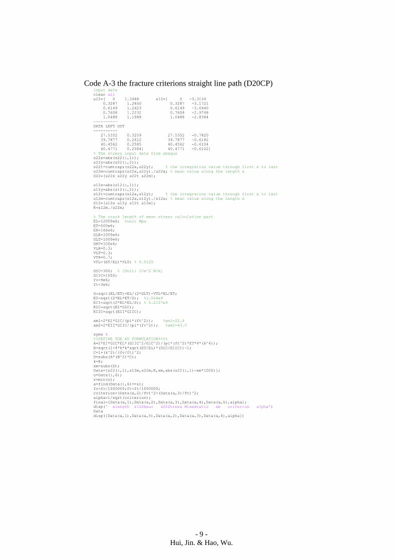
- 9 -
Hui, Jin. & Hao, Wu.
Code A-3 the fracture criterions straight line path (D20CP) Input date
clear all
s22=[ 0 1.3488 s12=[ 0 -3.3134
0.3287 1.2850 0.3287 -3.1721
0.6149 1.2423 0.6149 -3.0440
0.7608 1.2232 0.7608 -2.9748
1.0488 1.1988 1.0488 -2.8384
----------
DATA LEFT OUT
----------
27.5352 0.3259 27.5352 -0.7820
39.7877 0.2612 39.7877 -0.6182
40.4562 0.2585 40.4562 -0.6104
40.4771 0.2584] 40.4771 -0.6102]
% The stress input data from abaqus
s22x=abs(s22(:,1));
s22y=abs(s22(:,2));
s22t=cumtrapz(s22x,s22y); % the integration value through first x to last
s22m=cumtrapz(s22x,s22y)./s22x; % mean value along the length x
S22=[s22x s22y s22t s22m];
s12x=abs(s12(:,1));
s12y=abs(s12(:,2));
s12t=cumtrapz(s12x,s12y); % the integration value through first x to last
s12m=cumtrapz(s12x,s12y)./s12x; % mean value along the length x
S12=[s12x s12y s12t s12m];
K=s12m./s22m;
% The crack length of mean stress calculation part
EL=12000e6; %unit Mpa
ET=500e6;
ER=166e6;
GLR=1000e6;
GLT=1000e6;
GRT=100e6;
VLR=0.3;
VLT=0.3;
VTR=0.7;
VTL=(ET/EL)*VLT; % 0.0125
GIC=300; % [Unit: J/m^2 N/m]
GIIC=1050;
fv=9e6;
ft=3e6;
S=sqrt(EL/ET)+EL/(2*GLT)-VTL*EL/ET;
EI=sqrt(2*EL*ET/S); %1.064e9
EII=sqrt(2*EL*EL/S); % 5.2127e9
KIC=sqrt(EI*GIC);
KIIC=sqrt(EII*GIIC);
xm1=2*EI*GIC/(pi*(ft^2)); %xm1=22.6
xm2=2*EII*GIIC/(pi*(fv^2)); %xm2=43.0
syms k
%%DEFINE THE X0 FORMULATION%%%%
A=2*EI*GIC*EL*(GIIC^2/GIC^2)/(pi*(ft^2)*ET*4*(k^4));
B=sqrt(1+4*k*k*sqrt(ET/EL)*(GIC/GIIC))-1;
C=1+(k^2)/(fv/ft)^2;
D=subs(A*(B^2)*C);
k=K;
xm=subs(D);
Data=[s22(:,1),s12m,s22m,K,xm,abs(s22(:,1)-xm*1000)];
u=Data(:,6);
z=min(u);
a=find(Data(:,6)==z);
fv=fv/1000000;ft=ft/1000000;
criterion=(Data(a,2)/fv)^2+(Data(a,3)/ft)^2;
alpha=1/sqrt(criterion);
final=[Data(a,1),Data(a,2),Data(a,3),Data(a,4),Data(a,5),alpha];
disp(' xlength s12Shear s22Stress Mixedratio xm criterion alpha')
Data
disp([Data(a,1),Data(a,5),Data(a,2),Data(a,3),Data(a,4),alpha])
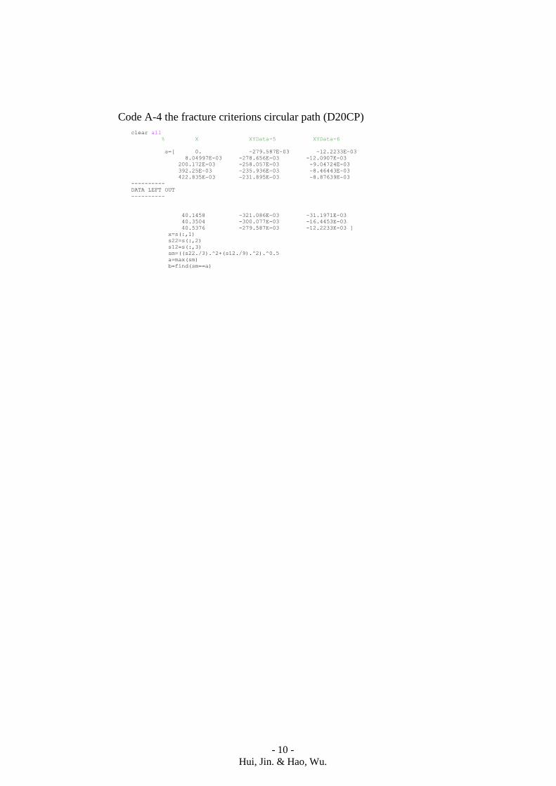
- 10 -
Hui, Jin. & Hao, Wu.
Code A-4 the fracture criterions circular path (D20CP)
clear all
% X XYData-5 XYData-6
s=[ 0. -279.587E-03 -12.2233E-03
8.04997E-03 -278.656E-03 -12.0907E-03
200.172E-03 -258.057E-03 -9.04724E-03
392.25E-03 -235.936E-03 -8.46443E-03
422.835E-03 -231.895E-03 -8.87639E-03
----------
DATA LEFT OUT
----------
40.1458 -321.086E-03 -31.1971E-03
40.3504 -300.077E-03 -16.4453E-03
40.5376 -279.587E-03 -12.2233E-03 ]
x=s(:,1)
s22=s(:,2)
s12=s(:,3)
sm=((s22./3).^2+(s12./9).^2).^0.5
a=max(sm)
b=find(sm==a)

Faculty of Technology 351 95 Växjö, Sweden Telephone: +46 772-28 80 00, fax +46 470-832 17 (Växjö)