finite element model for brittle fracture and fragmentation · ... a phantom node method, which is...

BNL-112403-2016-JA

Finite Element Model for Brittle Fracture and

Fragmentation

Wei Li1, Tristan J. Delaney

1, Xiangmin Jiao

1,

Roman Samulyak 1,2

, Cao Lu1

1Dept. of Applied Mathematics & Statistics, Stony Brook University, Stony

Brook NY 11794, USA 2 Brookhaven National Laboratory, Upton, NY 11973 USA

Submitted to Procedia Computer Science

June 2016

Computational Science Initiative

Brookhaven National Laboratory

U.S. Department of Energy [USDOE Office of Science]

[Advanced Scientific Computing Research]

Notice: This manuscript has been co-authored by employees of Brookhaven Science Associates, LLC under

Contract No. DE-SC0012704 with the U.S. Department of Energy. The publisher by accepting the

manuscript for publication acknowledges that the United States Government retains a non-exclusive, paid-up,

irrevocable, world-wide license to publish or reproduce the published form of this manuscript, or allow others

to do so, for United States Government purposes.

DISCLAIMER

This report was prepared as an account of work sponsored by an agency of the

United States Government. Neither the United States Government nor any

agency thereof, nor any of their employees, nor any of their contractors,

subcontractors, or their employees, makes any warranty, express or implied, or

assumes any legal liability or responsibility for the accuracy, completeness, or any

third party’s use or the results of such use of any information, apparatus, product,

or process disclosed, or represents that its use would not infringe privately owned

rights. Reference herein to any specific commercial product, process, or service

by trade name, trademark, manufacturer, or otherwise, does not necessarily

constitute or imply its endorsement, recommendation, or favoring by the United

States Government or any agency thereof or its contractors or subcontractors.

The views and opinions of authors expressed herein do not necessarily state or

reflect those of the United States Government or any agency thereof.

Finite Element Model for Brittle Fracture and

Fragmentation

Wei Li1, Tristan J. Delaney1, Xiangmin Jiao1, Roman Samulyak12∗, and Cao Lu1

1 Dept. of Applied Mathematics & Statistics, Stony Brook University, Stony Brook, NY 11794, USA{wei.li,tristan.delaney,xiangmin.jiao,roman.samulyak,cao.lu}@stonybrook.edu2 Computational Science Initiative, Brookhaven National Laboratory, Upton, NY 11973

AbstractA new computational model for brittle fracture and fragmentation has been developed basedon finite element analysis of non-linear elasticity equations. The proposed model propagatesthe cracks by splitting the mesh nodes alongside the most over-strained edges based on theprincipal direction of strain tensor. To prevent elements from overlapping and folding underlarge deformations, robust geometrical constraints using the method of Lagrange multipliershave been incorporated. The model has been applied to 2D simulations of the formation andpropagation of cracks in brittle materials, and the fracture and fragmentation of stretched andcompressed materials.

Keywords: brittle fracture, fragmentation, collision detection, finite elements method, nonlinear elas-

ticity

1 Introduction

Computational study of brittle fracture networks are of great interest to engineers who workwith material that breaks before it can undergo plastic deformation. This can occur when thematerial is in a “pre-stressed” configuration, where small deformations and strains can lead thematerial to surpass its internal critical stress. Of great importance to engineers is the predictionof crack nucleation and overall dependence of the resulting crack pattern on material properties.

Computational methods are of growing importance in modeling brittle fracture in materials.Due to the complex nature of fracture mechanics, several phenomenological methods have beenproposed. Such methods include generalized and extended finite element methods (X-FEM)[8, 11], cohesive element (CE) models [2], and spring models [9].

The extended FEM (X-FEM) [11] and the generalized FEM (GFEM) [12], which are closelyrelated and both belong to the partition of unity methods (PUM) [8], enrich the traditionalFEM function space with families of discontinuous shape functions, which can model the dis-placements of either the crack tip or opposite sides of the crack plane. The main advantage lies

∗Corresponding author.

FEM for Brittle Fracture and Fragmentation W. Li, T. J. Delaney, X. Jiao, R. Samulyak, and C. Lu

in the fact that the interface can be studied within each individual element without having toconstantly remesh near the crack tip. The types of enrichment functions can model a varietyof engineering problems the crack tip including branching [6], material interfaces, and soft dis-continuities. More recently, a phantom node method, which is a variant of the extended FEMwas developed in [?].

Cohesive zone models (CZM) were first introduced by Barenblatt [2] and have been incor-porated into commercial FEM codes. The CZM is intriguing because it explicitly avoids thecreation of stress singularities by modeling inter-element traction-displacement relationships.Elements become separated when their tractions exceed a critical threshold, and the locationof the “cohesive elements” (CE) can generate complex fracture networks. Cohesive elementshave been used in traditional finite element codes by Xu and Needleman [16] and Ortiz and Ca-macho [5]. Additionally, cohesive zone models have been incorporated into other finite elementframeworks such as X/G-FEM [11], meshless methods [1], and isogeometric analysis [13]. WhileCZMs may provide complex fracture structures, it was noted in [7] that CZMs are dependenton aspects of the mesh.

Spring models were introduced in [4, 10] and have the advantage of very simple implemen-tation of solid mechanics and fracture mechanics. For example, Meakin [10] modeled fractureusing a two-dimensional network of springs with a critical tension parameter. Over-strainedsprings were removed to simulate the propagation of fracture. Beale added random defects andperturbations to a spring model to investigate their effects on the propagation of the crack sur-face [4]. However, both of these models implemented fracture mechanisms by removing springs;thereby losing mass conservation and “obliterating” material under compression.

Recently, Wei et al. [9] investigated the use of mass conservative spring models, and wereable to reproduce complex fracture networks in two and three dimensions. The method usednonlinear optimization of the global energy functional and split vertices adjacent to springs thatwere strained past a pre-defined threshold. The advantage of this method was that it conservedmass and produced rich crack networks throughout the material. The work demonstratedcomplex fracture patterns, which qualitatively change due to variations in material properties.

The spring network model of [9] is difficult to integrate into pre-existing finite elementsoftware. The intent of this paper is to apply the fracture mechanisms of [9] to existing finiteelement codes. In this work, we describe the fracture mechanism incorporated into a finiteelement solid mechanics code as well as collision detection algorithms to prevent inter-elementpenetration.

The remainder of the paper is divided as follows. In Section 2, the principles of continuummechanics and their implementation within the finite element method are briefly discussed.In Section 3, the fracture mechanism is described, and particular emphasis is placed on thedetection of intersecting elements and their resolution through the introduction of Lagrangemultipliers. In Section 4, we present some verification of our FEM code and simulation resultswith our fracture model. Finally, we present concluding remarks in Section 5.

2 Finite Element Based Brittle Fracture Model

Finite element analysis is an important tool in the study of solid mechanics and fracture me-chanics in particular. Linear elastic fracture mechanics (LEFM) has been well-studied usingmethods such as X-FEM and CZM. However, the range of applications of LEFM is limited bythe assumptions of linear elasticity, which is valid for small displacements and small strains.In many applications involving brittle fracture, large displacements and rotations may occurwhile the strain exhibited within a material may still be in the elastic regime. Therefore, it is

2


important to take into account these geometric nonlinearities in the continuum formulation. Inparticular, we use a quasi-static updated Lagrangian description of the physical system followingthat in [3].

For any solid body of some material, denoted at time τ as τV , the material is in energeticequilibrium when the principle of virtual work is satisfied, namely that the body is in a minimumenergy configuration. The principle of virtual work for a body at some future time t+ ∆t canbe written as [3] ∫

t+∆tV

t+∆tτijδt+∆teijt+∆tdv = t+∆tR, (1)

where t+∆tτij is the Cauchy stress tensor of the material, δt+∆teij is the linear variation oflinear strain tensor at time t + ∆t, and t+∆tR is the total sum external virtual work due tosurface tractions and body forces.

Since the configuration of the body at time t+ ∆t is unknown, (1) cannot be solved directlyand instead must be rewritten in term of some previously known configuration. In the updatedLagrangian formulation, (1) may be rewritten in terms of the material body in its currentconfiguration at time t,∫

tVtCijrs tεrsδ tεij

tdv +

∫tV

tτijδtηijtdv = t+∆tR −

∫tV

tτijδteijtdv, (2)

which is a nonlinear equation in the incremental nodal displacements ui.

The nonlinear equation (2) can be solved using an iterative method. We choose to usethe modified Newton-Raphson scheme of [3] to iteratively determine the solution of (2). Inparticular, the stiffness matrix associated with (2) is computed only once and is held con-stant throughout the Newton-Raphson iteratin. Lagrange multipliers are used to accommodateseveral types of (linear) Dirichlet boundary conditions on the vertex displacement degrees offreedom, ui. We solve (2) iteratively by solving for several incremental displacements of theform [

tK GT

G 0

] [∆u(k)

λ

]=

[t+∆tR − t+∆t

t+∆tF(k−1)

b(k−1)

], (3)

where tK is the tangent stiffness matrix of the body in configuration tV , t+∆tt+∆tF

(k−1) is the

internal virtual work of the deformed body in configuration t+∆tV (k−1). Within each step ofthe Newton-Raphson iteration, the nodal displacements are updated as

t+∆tu(k+1)i = t+∆tu

(k)i + ∆u

(k+1)i , (4)

t+∆tu(0)i = tui. (5)

The vector of Dirichlet conditions, b(k−1), is updated within each iteration to ensure thateach incremental displacements enforce the correct boundary conditions at each increment. Theupdate is computed via

b(k−1) = b−G t+∆tu(k−1). (6)

As the nodal displacements t+∆tu(k−1)i are updated, the internal virtual work of the current

updated configuration, t+∆tt+∆tF

(k−1), is updated and subtracted from the external virtual work.

At each increment, (3) is solved using an incomplete LU-preconditioned GMRES solver,which is available in MATLAB and PETSc. The iteration stops once the vector of incremental

3


nodal displacements is within a predefined tolerance∥∥∆u(k)∥∥

2∥∥∆u(0)∥∥

2

< tol. (7)

3 Crack Formation and Propagation Algorithm

The cracks form and propagate when some part of the brittle material exceeds its critical strain.In the network based model, the overstrained bonds are split [9]. In the FEM based approach,we split overstrained nodes and generate new edges to introduce cracks. In order to determinethe overstrained nodes, we calculate the nodal strain tensor by averaging the value of strainsfrom the neighboring elements. The principal strain is the largest eigenvalue of the straintensor, and its eigenvector is the maximum strain direction. We collect a set of overstrainednodes by comparing their principal strains with the fracture critical strain threshold. For eachoverstrained node, we split edges that are most orthogonal to the maximum strain direction.Depending on the location of the node, we propose some rules:

1. If a node u1 is an interior node, we split two edges with minimum angles to the orthogonaldirection of the maximum strain. u1 is the splitting end of the two edges.

(a) If the two edges belong to the same element, we will discard one with a larger angleand pick a different edge.

(b) If the other end of a chosen edge, vertex u2, is on the boundary or crack surface,u2 will also be a splitting end. This is to prevent the case where two chunks areconnected by a single vertex.

2. If a node v1 is a boundary node, we select one edge with the minimum angle to theorthogonal direction of the maximum strain.

(a) If the chosen edge is an interior edge, v1 will be the splitting end. Otherwise, noedge will be split.

(b) Similar to case 1 if the other end of the chosen edge, vertex v2, is on the boundaryor crack surface, v2 will also be a splitting end.

After each node is processed, we update the element connectivity list and other related datastructures, as is shown in Figure 1.

3.1 Collision Detection

When cracks form and the mesh breaks into fragments, the mesh may fold and the fragmentsmay overlap, creating unphysical states. Introduction of proper constraints resolves this issue.It provides a physics-based interaction model between fragments and the cracked material andleads to the propagation of cracks.

Before elimination, the overlapping and folding should be detected first. A standard wayis to do pairwise triangles collision detection, in which triangles have at least one edge oncrack surface. In order to reduce the number of pairwise comparison, the computational field isdivided into coarse grids, and elements are assigned to each grid based on where the coordinatesof their center fall into.

4


max strain

u1u1

u′1max strain

u1

(a) Case 1a

max strain

u1u1

u′1

u2 u2u′2

(b) Case 1b

v1 v1v′1

max strain

(c) Case 2a

v1 v1v′1

v2 v2v′2

max strain

(d) Case 2b

Figure 1: Illustrations of the mesh splitting process.

The detection process sweeps from upper left corner grid block towards lower right cornergrid block, and only elements in right, lower or right lower diagonal adjacent grid would bedetected pairwise for each grid block.

For each pair of triangles, first of all, every vertex of each element is examined if it is insideof the other one. This step checks 6 vertices using relative coordinates within each triangle,and would preclude succeeding examinations in most overlapping situations. However, thereare cases that triangles are just intersecting each other by edges, thus, we need to check edge-to-edge intersections pair-wisely, and this line segments intersection checking happens between9 pairs.

In cases of stiff material, both the deformation and the overlapped parts are very small. Theround-off error makes it difficult to assert whether these elements are overlapped. Presetting a“threshold” value helps to resolve this problem. By adding this controlling parameter to thealgorithm, we adjust the precision of the overlap detection. This is crucial for the simulationbecause adding too few constraints would impair the correct physical system we would liketo obtain, while adding too many constraints would result in an over-determined state of thesystem, eventually leading to a failure.

3.2 Contact Constraints

For frictionless contact problems, the contact condition, known as a Kuhn-Tucker condition,can be written as

gN ≤ 0, pN ≤ 0 on Γc, gNpN = 0, (8)

where gN is the normal component of the gap function, and pN is the normal component ofcontact stress.

We adopt the method of Lagrangian multipliers to resolve the contact problem. The contactcontribution and its variation can be written as:

Πc =

∫Γc

λNgN dA, Cc =

∫Γc

(λNδgN + δλNgN ) dA, , (9)

where λN denotes the Lagrangian multiplier which can be identified as the contact pressure pN ,and δgN is the variation of the normal contact gap function [14]. The Lagrangian multipliers

5


add constraints contribution to the weak formulation of the solids in contact, and preventfurther penetration between overlapping elements and push already overlapped triangles backto separated status.

Equation (9) can be generally discretized by introducing discretization for the gap functionin each contact area Γic, that

giN = CiTu, C = [C1|C2|...|Cns ], Λ = (λ1, λ2, ..., λns), (10)

which C depends on the choice of discretization, thus∫Γc

λNgN dA → ΛTCTu,

∫Γc

λNδgN dA → δuTCΛ,

∫Γc

δλNgN dA → δΛTCu, (11)

The constraints can be arranged into the KKT matrix as (t+∆ttKL + t+∆t

tKNL

)GT CT

G 0 0C 0 0

uλDλc

=

R − ttF

bgc

, (12)

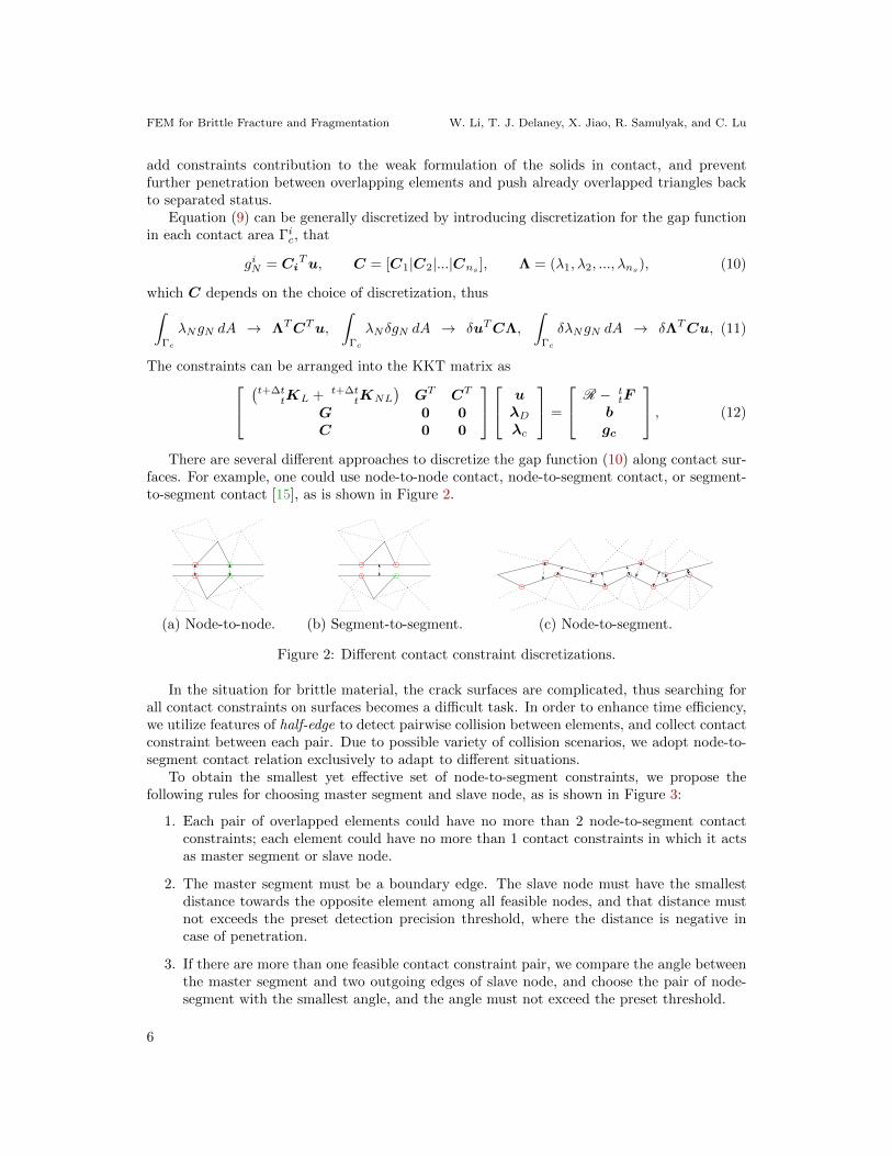
There are several different approaches to discretize the gap function (10) along contact sur-faces. For example, one could use node-to-node contact, node-to-segment contact, or segment-to-segment contact [15], as is shown in Figure 2.

(a) Node-to-node. (b) Segment-to-segment. (c) Node-to-segment.

Figure 2: Different contact constraint discretizations.

In the situation for brittle material, the crack surfaces are complicated, thus searching forall contact constraints on surfaces becomes a difficult task. In order to enhance time efficiency,we utilize features of half-edge to detect pairwise collision between elements, and collect contactconstraint between each pair. Due to possible variety of collision scenarios, we adopt node-to-segment contact relation exclusively to adapt to different situations.

To obtain the smallest yet effective set of node-to-segment constraints, we propose thefollowing rules for choosing master segment and slave node, as is shown in Figure 3:

1. Each pair of overlapped elements could have no more than 2 node-to-segment contactconstraints; each element could have no more than 1 contact constraints in which it actsas master segment or slave node.

2. The master segment must be a boundary edge. The slave node must have the smallestdistance towards the opposite element among all feasible nodes, and that distance mustnot exceeds the preset detection precision threshold, where the distance is negative incase of penetration.

3. If there are more than one feasible contact constraint pair, we compare the angle betweenthe master segment and two outgoing edges of slave node, and choose the pair of node-segment with the smallest angle, and the angle must not exceed the preset threshold.

6


4. If all above rules does not satisfy, there will be no constraints subscribed for the givenpair of overlapped elements.

(a) 2 constraints per pair. (b) Choose the smallest gap. (c) Choose the smallest angle.

Figure 3: Rules on choosing contact.

The Lagrangian Multipliers are obtained in a predict-and-correct manner, which use pre-dicted position without contact constraints for both node xb and segment (xa, xc) to calculatethe surface norm n and the gap function gN , which are calculated in the following steps:

1. Project slave node xb on the master edge (xa, xc) as x′b and calculate ξ

x′b = ξxa + (1− ξ)xc, (x′b − xb) · (xa − xc) = 0. (13)

2. Calculate the normal gap distance as a linear relation for displacement ua, ub, uc

gN = (ξ(xa + ua) + (1− ξ)(xc + uc)− (xb + ub)) · nd. (14)

3. Assemble the coefficient of u into C and constant into gc in (12).

As is shown in Figure 4, this node-to-segment contact will reduce to a node-to-node contactif ξ is 0 or 1 in some cases.

gN

xb;ub

xa;ua

xc;uc

x′b

Figure 4: Contact constraint calculation.

eA

eB

eC

Figure 5: Redundant constraints.

Even if we apply these rules to how contact constraints are added, there could still benumerous duplicate or redundant contact constraints. For example, a duplicate constraintoccurs when adding degenerated node-to-segment contact, which is essentially a node-to-nodecontact, that the slave node is exactly the same vertex sharing by adjacent elements. Redundantconstraints occur when the mesh breaks up totally at one vertex, when 3 or more elements arein node-to-node contact with one another, and vertices constraints between va and vc may be

7


derived from constraints between va and vb, and constraints between vb and vc, as shown inFigure 5

Redundant constraints would result in a singular or badly conditioned KKT system. Toresolve the problem, we firstly collect all contact constraints and apply QR factorization toextract the largest linear independent rows from the contact constraints matrix. After that, weadd the deducted contact constraint matrix C to the KKT system.

4 Numerical Results

In this section, we present several numerical results with the proposed finite-element fracturemodel. We start with a verification of the FEM code for linear elasticity, and then presentresults for the fracture model.

4.1 Verification of the Finite Element Code

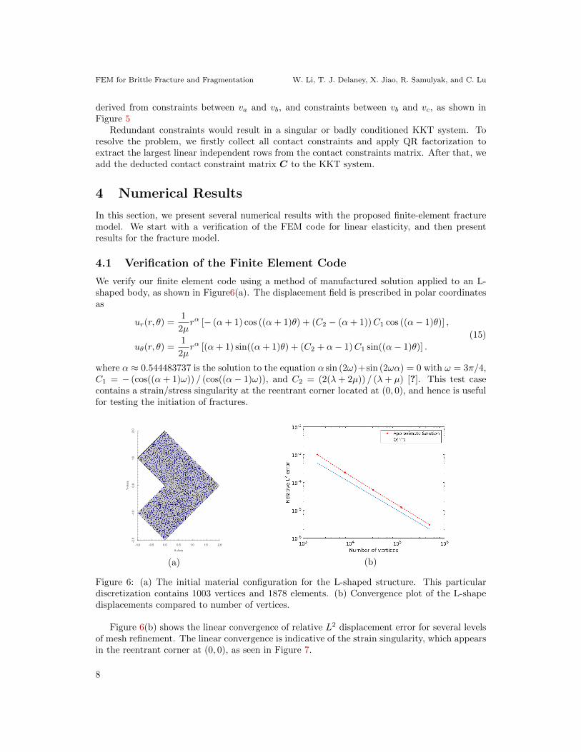
We verify our finite element code using a method of manufactured solution applied to an L-shaped body, as shown in Figure6(a). The displacement field is prescribed in polar coordinatesas

ur(r, θ) =1

2µrα [− (α+ 1) cos ((α+ 1)θ) + (C2 − (α+ 1))C1 cos ((α− 1)θ)] ,

uθ(r, θ) =1

2µrα [(α+ 1) sin((α+ 1)θ) + (C2 + α− 1)C1 sin((α− 1)θ)] .

(15)

where α ≈ 0.544483737 is the solution to the equation α sin (2ω)+sin (2ωα) = 0 with ω = 3π/4,C1 = − (cos((α+ 1)ω)) / (cos((α− 1)ω)), and C2 = (2(λ+ 2µ)) / (λ+ µ) [?]. This test casecontains a strain/stress singularity at the reentrant corner located at (0, 0), and hence is usefulfor testing the initiation of fractures.

(a) (b)

Figure 6: (a) The initial material configuration for the L-shaped structure. This particulardiscretization contains 1003 vertices and 1878 elements. (b) Convergence plot of the L-shapedisplacements compared to number of vertices.

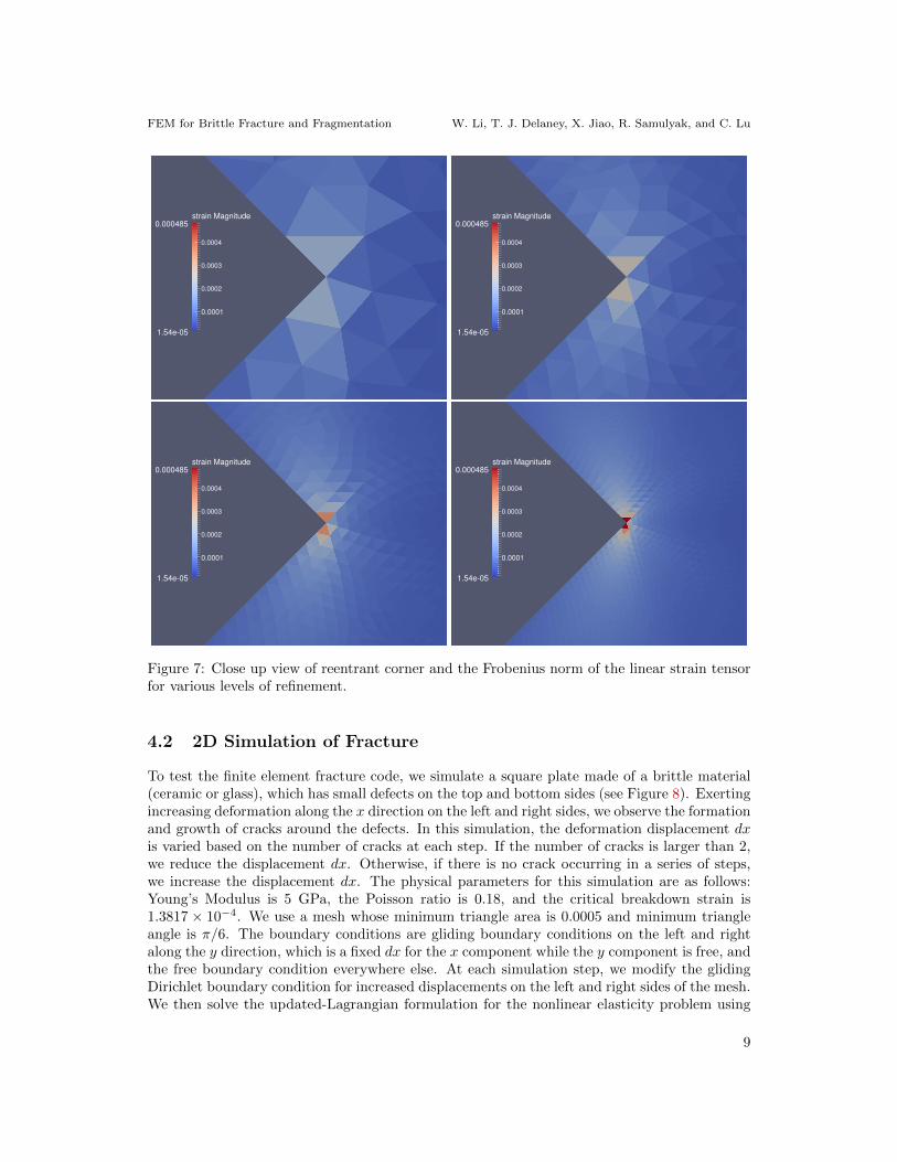
Figure 6(b) shows the linear convergence of relative L2 displacement error for several levelsof mesh refinement. The linear convergence is indicative of the strain singularity, which appearsin the reentrant corner at (0, 0), as seen in Figure 7.

8


0.0001

0.0002

0.0003

0.0004

strain Magnitude

1.54e-05

0.000485

0.0001

0.0002

0.0003

0.0004

strain Magnitude

1.54e-05

0.000485

0.0001

0.0002

0.0003

0.0004

strain Magnitude

1.54e-05

0.000485

0.0001

0.0002

0.0003

0.0004

strain Magnitude

1.54e-05

0.000485

Figure 7: Close up view of reentrant corner and the Frobenius norm of the linear strain tensorfor various levels of refinement.

4.2 2D Simulation of Fracture

To test the finite element fracture code, we simulate a square plate made of a brittle material(ceramic or glass), which has small defects on the top and bottom sides (see Figure 8). Exertingincreasing deformation along the x direction on the left and right sides, we observe the formationand growth of cracks around the defects. In this simulation, the deformation displacement dxis varied based on the number of cracks at each step. If the number of cracks is larger than 2,we reduce the displacement dx. Otherwise, if there is no crack occurring in a series of steps,we increase the displacement dx. The physical parameters for this simulation are as follows:Young’s Modulus is 5 GPa, the Poisson ratio is 0.18, and the critical breakdown strain is1.3817 × 10−4. We use a mesh whose minimum triangle area is 0.0005 and minimum triangleangle is π/6. The boundary conditions are gliding boundary conditions on the left and rightalong the y direction, which is a fixed dx for the x component while the y component is free, andthe free boundary condition everywhere else. At each simulation step, we modify the glidingDirichlet boundary condition for increased displacements on the left and right sides of the mesh.We then solve the updated-Lagrangian formulation for the nonlinear elasticity problem using

9


the quasi- Newton method. A crack processing routine is applied to the mesh to open cracksaround overstrained nodes, based on the principal direction of the stress tensor of the node,while the stress is an averaged value from the vertex’s surrounding elements. To ensure thesystem’s finite element discretized virtual work plus Lagrangian multiplier matrix to be non-singular or not badly scaled, we add extra boundary conditions for isolated elements. In ourcurrent case, because of lacking contact constraint of elements touching each other, we onlyplaced two fixed points for each isolated piece of glass. In the end, we check if the crack numberexceeds the maximum number of cracks prescribed. If so, we reduce the displacements dx atone step and re-run the procedure using the old data; otherwise we keep the deformation to beunchanged and run step 2 and 3 for a release of energy through crack formation until there areno more cracks occurring. Figure 8 shows some sample results of the fracture of a brittle plateunder tension.

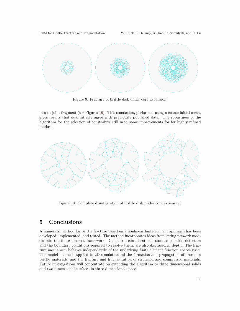
To test the robustness of the model, we simulate a brittle disk that has a hole in the center.The hole is in contact with an expanding softer material core, which is not displayed; see Figures9. While exerting increasing expansion on the inner core, which is passed by contact conditiontowards the outer disk, cracks begin to form around the hole. The applied deformation of theinner core is such that the inner part of the disk completely disintegrates into grains, formingthe so-called comminuted zone, while the outer part of the disk remains intact.

Under increased deformation of the inner core, the disk undergoes complete disintegration

Figure 8: Fracture of brittle plate under tension.

10


Figure 9: Fracture of brittle disk under core expansion.

into disjoint fragment (see Figures 10). This simulation, performed using a coarse initial mesh,gives results that qualitatively agree with previously published data. The robustness of thealgorithm for the selection of constraints still need some improvements for for highly refinedmeshes.

Figure 10: Complete disintegration of brittle disk under core expansion.

5 Conclusions

A numerical method for brittle fracture based on a nonlinear finite element approach has beendeveloped, implemented, and tested. The method incorporates ideas from spring network mod-els into the finite element framework. Geometric considerations, such as collision detectionand the boundary conditions required to resolve them, are also discussed in depth. The frac-ture mechanism behaves independently of the underlying finite element function spaces used.The model has been applied to 2D simulations of the formation and propagation of cracks inbrittle materials, and the fracture and fragmentation of stretched and compressed materials.Future investigations will concentrate on extending the algorithm to three dimensional solidsand two-dimensional surfaces in three-dimensional space.

11


Acknowledgements The authors would like to thank Prof. James Glimm and Dr. MichaelGreenfield for insightful discussions. Research was partially supported by US Army ResearchOffice under contracts #W911NF0910306 and GS04T09DBC0017.

References

[1] E. Barbieri and M. Meo. A meshless cohesive segments method for crack initialization and prop-agation in composites. Advanced Composite Materials, 18(1):45–63, 2011.

[2] G. I. Barenblatt. The mathematical theory of equilibrium cracks in brittle fracture. Advances inApplied Mechanics, 7(1):55–129, 1962.

[3] K.-J. Bathe, E. Ramm, and E. Wilson. Finite element formulations for large deformation dynamicanalysis. Int. J. Numer. Meth. Engrg., 9:353–386, 1975.

[4] P. D. Beale and D. J. Srolovitz. Elastic fracture in random materials. Physical Review B,37(10):5500, 1988.

[5] G. T. Comacho and O. M. Computational modeling of impact damage in brittle materials. Inter-national Journal of Solids and Structures, 33(20):2899–2938, 1996.

[6] C. Daux, N. Moes, J. Dolbow, N. Sukumar, and T. Belytschko. Abritrary branched and intersectingcracks with the extended finite element method. Int. J. Numer. Meth. Engrg., 48:1741–1760, 2000.

[7] R. De Borst. Numerical aspects of cohesive-zone models. Engineering Fracture Mechanics,70(14):1743–1757, 2003.

[8] T.-P. Fries and T. Belytschko. The extended/generalized finite element method: An overview ofthe method and its applications. Int. J. Numer. Meth. Engrg., 84:253–304, 2010.

[9] R. S. H. Wei. Mass-conservative network model for brittle fracture, 2014.

[10] P. Meakin, G. Li, L. Sander, E. Louis, and F. Guinea. A simple two-dimensional model for crackpropagation. Journal of Physics A: Mathematics and General, 22(9):1393, 1989.

[11] N. Moes and T. Belytschko. Extended finite element method for cohesive crack growth. EngineeringFracture Mechanics, 69:813–833, 2002.

[12] J. Pereira, C. A. Duarte, and X. Jiao. Three-dimensional crack growth with hp-generalized finiteelement and face-offsetting methods. Computational Mechanics, 46(3):431–453, 2010.

[13] C. V. Verhoosel, M. A. Scott, R. de Borst, and T. J. Hughes. An isogeometric approach to cohesivezone modelling. Int. J. Numer. Meth. Engrg., 87(1-5):336–350, 2011.

[14] P. Wriggers. Finite element algorithms for contact problems. Archives of Computational Methodsin Engineering, 2,4:1–49, 1995.

[15] P. Wriggers. Computational Contact Mechanics, chapter 6-9, pages 109–182. Springer-Verlag,Berlin, 2006.

[16] X.-P. Xu and A. Needleman. Numerical simulations of fast crack growth in brittle solids. Journalof the Mechanics and Physics of Solids, 42(9):1397–1434, 1994.

12

finite element model for brittle fracture and fragmentation · ... a phantom node method, which is...

Documents