finite element implementation of virtual internal...
TRANSCRIPT
Engineering Fracture Mechanics 71 (2004) 401–423
www.elsevier.com/locate/engfracmech
Finite element implementation of virtual internal bondmodel for simulating crack behavior
Ganesh Thiagarajan a, K. Jimmy Hsia b,*, Yonggang Huang c
a Department of Civil Engineering, University of Missouri-Kansas City, Kansas City, MO 64110, USAb Department of Theoretical and Applied Mechanics, University of Illinois at Urbana-Champaign, Urbana, IL 61801, USA
c Department of Mechanical and Industrial Engineering, University of Illinois at Urbana-Champaign, Urbana, IL 61801, USA
Received 10 January 2001; received in revised form 16 September 2002; accepted 21 January 2003
Abstract
The virtual internal bond (VIB) model has been recently proposed to describe material deformation and failure
under both static and dynamic loading. The model is based on the incorporation of a cohesive type law in a hyperelastic
framework, and is capable of fracture simulation as a part of the constitutive formulation. However, with an implicit
integration scheme, difficulties are often encountered in the finite element implementation of the VIB model due to
possible negative eigenvalues of the stiffness matrix. This paper describes the implementation of an explicit integration
scheme of the VIB model. Issues pertaining to the implementation, such as mesh size and shape dependence, loading
rate dependence, crack initiation and growth characteristics, and solution time are examined. Both quasi-static and
dynamic loading cases have been studied. The experimental validation of the VIB model has been done by calibrating
the model parameters using the experimental data of Andrews and Kim [Mech. Mater. 29 (1988) 161]. The simulations
using the VIB model are shown to agree well with the experimental observations.
� 2003 Elsevier Ltd. All rights reserved.
Keywords: Cohesive model; VIB model; Finite elements; Static and dynamic crack propagation; Explicit integration scheme
1. Introduction
Numerical simulations of crack initiation, propagation and branching are a computationally intensive
process. Traditional finite element packages simulate the crack propagation problem either by using sin-
gularity elements or by using line spring elements with built-in fracture criteria. Recently, a popular methodto do this task is the cohesive surface modeling of the fracture zone. Following the work of Barenblatt [2],
Dugdale [3], and Willis [4], many researchers have addressed the issues pertaining to this approach. Nee-
dleman [5] provided a framework for the separation process starting from initial debonding in the cohesive
zone. Larsson [6] used this approach to simulate crack growth in brittle materials, while Xia and Shih [7]
simulated fracture in ductile materials under static loading. Camacho and Ortiz [8] have used cohesive
* Corresponding author. Tel.: +1-217-333-2321; fax: +1-217-244-5707.
E-mail address: [email protected] (K.J. Hsia).
0013-7944/$ - see front matter � 2003 Elsevier Ltd. All rights reserved.
doi:10.1016/S0013-7944(03)00102-4
402 G. Thiagarajan et al. / Engineering Fracture Mechanics 71 (2004) 401–423
surface modeling to study material fragmentation, while Xu and Needleman [9] used it to study dynamic
crack tip instabilities by allowing cracks to form along element boundaries. The method by Xu and
Needleman involves introducing special boundary elements between regular elements, where the boundary
elements obey a cohesive law. Three factors influence the cohesive law behavior, namely the cohesivestrength, the critical separation at cohesive strength and the fracture energy in the separation process. These
models obviate the need for a separate external fracture criterion in fracture simulations. The effects of
plasticity inside volumetric elements have been investigated using the embedded-process-zone cohesive
fracture model by Tvergaard and Hucthinson [10,11]. Gullerud and Dodds [12] have used 3-D cohesive
elements for modeling ductile crack growth. More recently Foulk et al. [13] presented a procedure for
implementing the cohesive zone model in a 3-D finite element framework where zones of cracking are
known a-priori and cohesive zone elements are placed along these element boundaries.
Gao [14,15] proposed that materials undergoing brittle fracture have large non-linear elastic deforma-tions and that a hyperelastic description of the crack tip behavior provides a better explanation of dynamic
crack tip instabilities. Gao and Klein [16] developed a method, called the virtual internal bond (VIB) model,
in which a cohesive type law is directly incorporated into the constitutive model. This is done by treating the
body as a collection of randomly distributed material points interconnected by a network of cohesive
bonds. The Cauchy–Born rule of crystal elasticity is used to derive the overall constitutive relations. This is
done by equating the strain energy of the bonds to the potential energy stored in the continuum due to
applied loads and deformations. As this is implemented in a hyperelastic framework of finite deformation
continuum mechanics, the Green–Lagrange strain tensor can be evaluated from deformation gradient, andthe second Piola–Kirchoff stress tensor can be computed from the potential energy expression. The main
advantage of this method is that, as in the cohesive boundary element approach [9], no separate fracture
criterion is needed. Furthermore, the cohesive law is now embedded directly into the constitutive equations,
thus no special boundary elements between regular elements are needed.
The application of the VIB model to fracture initiation and dynamic crack propagation was shown by
Klein and Gao [17]. An implicit second order time stepping algorithm was used for the simulations. They
successfully simulated both quasi-static and dynamic loading problems. Zhang et al. [18] presented a nu-
merical algorithm, using the implicit integration scheme, for the VIB model under static loading cases andimplemented the material model in ABAQUS 1 using the UMAT subroutine.
One of the primary issues in implementing constitutive models with a cohesive formulation is the
softening region, which often causes problems in the stability of numerical simulations. The VIB formu-
lation also correlates the onset of fracture to the presence of strain localization, arising from the loss of
ellipticity of the governing equations and posing a number of difficulties in the implicit integration scheme
for static problems. The difficulties are in the form of singular tangent stiffness matrix and presence of
highly negative eigenvalues, resulting possibly in the failure to converge to any solution at all. Thus the
successful execution of the implicit scheme requires preconditions such as the incorporation of high stiffnesselements adjoining the VIB layer of elements [16] or specifying a narrow band of VIB layer which is akin to
prespecifying the crack path [18]. These difficulties have also been observed by the present researchers.
The motivation for the present work stems from the desire to implement a robust formulation of the VIB
model without any preconditions attached. The problem thus leads to an alternative formulation, namely
the usage of explicit integration schemes. Albeit being slow to converge, the explicit integration schemes
avoid difficulties arising from the loss of ellipticity of the governing equations due to the stabilizing effects
of the mass matrix. However, explicit schemes, if not used judiciously, could pose problems relating to the
convergence to the true solution. Issues that could affect convergence, especially when simulating staticloading in a dynamic environment, are the influence of mesh shape and size, loading rate and history, and
1 Commercial FE program from HKS Inc.

G. Thiagarajan et al. / Engineering Fracture Mechanics 71 (2004) 401–423 403
material parameters, amongst others. An appropriate choice of time step and increments is also required to
accurately simulate static loading cases.
The work presented here attempts to implement the VIB model in an explicit integration scheme and to
study the robustness of it by examining in detail the issues outlined in the previous paragraph. Both thequasi-static loading case, in the form of crack initiation and propagation in a plate with a hole subjected to
uniaxial tension, and the dynamic loading case, in the form of impact of a deformable disk on a rigid wall,
are studied.
Andrews and Kim [1] studied the dynamic fragmentation of brittle materials experimentally by im-
pacting small spherical (0.4–6.35 mm in radius) alumina balls against a rigid anvil. The impact process was
observed using high speed cameras. It was experimentally observed that the threshold impact velocity,
defined as the velocity at which the ball rebounds with damage, depended on the material properties and the
ball diameter. In our numerical simulations the VIB model parameters are calibrated using one set of theirexperimental data and simulations are compared with the other sets of experiments. The predictions of our
simulations agree well with the experimental observations.
2. Elements of virtual internal bond model
A complete discussion of the VIB model is given in Gao and Klein [16] which is summarized below. The
basic premise on which the VIB model is built is that the elastic behavior of a spatial distribution ofmaterial points, arising as a result of microstructural cohesive bonds, can be described using the Cauchy–
Born rule of crystal elasticity. The interaction among the microstructural particles can be described through
interaction potentials. In a polycrystalline material, the material behavior is isotropic because of the ran-
dom crystallographic orientation of grains. Such behavior can be modeled by a random spatial distribution
of cohesive bonds using the VIB model.
The VIB model is described within the framework of hyperelastic continuum mechanics. The initial and
the deformed configurations are defined using the Lagrangian coordinates X ¼ XI and the Eulerian co-
ordinates x ¼ xðX; tÞ ¼ xiðXI ; tÞ, respectively. In this paper capital letter subscripts are used for the initialconfiguration while lower case subscripts are used for the deformed configuration. The deformation gra-
dient can be expressed as
F ¼ ox
oXor FiI ¼
oxioXI
ð1Þ
The Green–Lagrange strain tensor can then be defined as
E ¼ 12ðFT � F� IÞ ð2Þ
where I is the second order identity tensor.
Consider an arbitrary microstructural bond at an angle h and /, where h is the angle of the bond ori-
entation with respect to the vertical positive z-axis, and / is the angle in the horizontal plane with respect tothe positive x-axis (in polar coordinates), respectively. The unit vector along this direction is given as
n ¼ ðsin h cos/; sin h sin/; cos hÞ with respect to the undeformed configuration. The stretch of this bond
can be given as
l ¼ l0ffiffiffiffiffiffiffiffiffiffiffiffiffiffiffiffiffiffiffiffiffiffiffiffiffi1þ 2nIEIJnJ
pð3Þ
The macroscopic strain energy density function is derived using the Cauchy–Born rule [19,20] as
wðEIJ Þ ¼ hUðlÞi ð4Þ
404 G. Thiagarajan et al. / Engineering Fracture Mechanics 71 (2004) 401–423
where h� � �i represents the weighted average with respect to the bond density function Dd . UðlÞ is the po-
tential energy function for each bond. Assuming that all bonds have the same initial length l0, for the
general case the weighted average is evaluated as,
h� � �i ¼Z 2p
0
Z p
0
� � �Ddðh;/Þ sin hdhd/ ð5Þ
The term Ddðh;/Þ sinðhÞdhd/ represents the number of bonds per unit volume between the bond angles
(h; hþ dh) and (/;/þ d/). As we restrict this study to isotropic solids the bond density function is taken asa constant D0. Hence the macroscopic strain energy density function can now be given as
wðEIJ Þ ¼ D0
Z 2p
0
Z p
0
UðlÞ sin hdhd/ ð6Þ
For a 2-dimensional isotropic solid subjected to plane stress the bond density function can be expressed asDddðh� p
2Þ and the strain energy density function becomes
w ¼ D0
Z 2p
0
UðlÞd/ ð7Þ
where d is the Dirac delta function.
2.1. Constitutive equations
From the strain energy density function w, the symmetric second Piola–Kirchoff stress SIJ and the elastic
modulus AIJKL can be derived as follows:
S ¼ owoE
or SIJ ¼owoEIJ
ð8Þ
AIJKL ¼o2w
oEIJ oEKLð9Þ
The modulus derived from this potential satisfies the major and minor symmetries, AIJKL ¼ AJIKL ¼AIJLK ¼ AKLIJ , as well as the Cauchy symmetry, AIJKL ¼ AIKJL. This results in only one isotropic elastic
constant being needed. This is due to the fact that the Cauchy symmetry is satisfied by the fourth order
isotropic elasticity tensor only for the case of k ¼ l, where k and l are the two Lam�ee constants.
2.2. Special cases
While it is impossible to derive a closed form solution for the elastic stiffness tensor for a general case,
Gao and Klein [16] have derived analytical forms of the elastic stiffness tensor for a few simple cases. Thesecases provide a guideline to correlate material properties to the model parameters. Three special cases of
interest are outlined below.
Infinitesimal strain: For this case the elastic tensor reduces to
AIJKL ¼ lðdIJdKL þ dIKdJL þ dILdKJ Þ ð10Þ
where dIJ is the Kronecker delta, and the shear modulus,
l ¼ 4p15
l20U00ðl0Þ ð11Þ
G. Thiagarajan et al. / Engineering Fracture Mechanics 71 (2004) 401–423 405
where U 00ðl0Þ is the second derivative of the potential energy function with respect to the bond length.
Poisson�s ratio for this case is a constant equal to 1/4. While this limits the suitability of the VIB model to
materials with Poisson�s ratio close to this value, it does cover a reasonable range of materials.
Plane strain equibiaxial stretching (finite deformation): This is the case that closely resembles the state ofstress near the mode I crack tip. The stiffness tensor components can be expressed in an integral form and it
was shown that the solid develops a transversely isotropic instantaneous response with a plane strain
Poisson�s ratio, given as A1122=A1111 (at finite deformation) of 1/3. The expressions for the elastic modulus
must be expressed in an integral form and is given in detail in [16].
Plane stress isotropic solid (finite deformation): This is a very useful case and is highly suitable for
implementation. It was shown by Gao and Klein [16] that the shear modulus is given by
l ¼ pD0l20U00ðl0Þ
4ð12Þ
while the elasticity tensor retains the same form as that in Eq. (10).
2.3. Cohesive force law
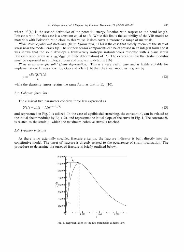
The classical two parameter cohesive force law expressed as
U 0ðlÞ ¼ Aaðl� l0Þe�ðl�l0Þ=Bb ð13Þ
and represented in Fig. 1 is utilized. In the case of equibiaxial stretching, the constant Aa can be related to
the initial shear modulus by Eq. (12), and represents the initial slope of the curve in Fig. 1. The constant Bb
is related to the strain at which the maximum cohesive stress is reached.
2.4. Fracture indicator
As there is no externally specified fracture criterion, the fracture indicator is built directly into the
constitutive model. The onset of fracture is directly related to the occurrence of strain localization. The
procedure to determine the onset of fracture is briefly outlined below.
l
U’(
l)
1 1.025 1.05 1.0750
2E+08
4E+08
6E+08
8E+08
1E+09
1.2E+09
1.4E+09
1.6E+09
Bb
Aa
Fig. 1. Representation of the two-parameter cohesive law.
406 G. Thiagarajan et al. / Engineering Fracture Mechanics 71 (2004) 401–423
The equation of motion in the initial configuration can be written as
oPiJoXJ
¼ qo2xiot2
ð14Þ
where PiJ is the asymmetric first Piola–Kirchoff stress given by the following transformation:
PiJ ¼ FiLSLJ ð15Þ
The effective tangent modulus in the mixed configuration is now given as
BiJkL ¼oPiJoFkL
ð16Þ
¼ dikSJL þ FiIAIJKLFkK ð17Þ
This is utilized in the classical condition of strain localization as follows. The acoustic tensor is defined as
QikðNÞ ¼ BiJkLNJNL ð18Þ
where N is a unit vector along the wave propagation direction. Strain localization is considered to occur
when the acoustic tensor becomes singular for a given N [21]. The loss of ellipticity of the acoustic tensor
signals the onset of fracture and is numerically used to detect it.Another way to define the onset of fracture is the strain at which the maximum cohesive stress is reached.
This critical strain is represented by the parameter Bb=I0 in Eq. (13). It is to be noted that this strain does
not necessarily coincide with the state at which strain localization takes place.
3. Finite element setup
The VIB model described above has been incorporated into a user material model subroutine in
ABAQUS. The implementation can be done using both implicit and explicit integration schemes. A brief
description of the implicit scheme [18] is given in Appendix C.
3.1. Explicit integration scheme
The major thrust of this paper is to study the performance of the VIB model with an explicit integration
scheme. The user material subroutine, VUMAT, is implemented using the Cauchy stress components. As
the stresses and strains are defined in the corrotational system, the stresses and other state variables can be
directly computed and updated in the subroutine. The steps to do this are outlined below. ABAQUSprovides, amongst other quantities, the strain increments and the deformation gradient at the current time
increment.
Step 1a: For the data check phase ABAQUS/Explicit calls VUMAT with a set of fictitious strains (at time
0.0). The data provided by VUMAT are used to calculate the initial elastic wave speeds and to
estimate the required initial time increment. During this phase the Green strain values are taken
from the input strain increments as
EIJ ¼ D�ij
D�ij ¼Z Dt
0
1
2ðLþ LTÞdt
ð19Þ
where L is the velocity gradient.
G. Thiagarajan et al. / Engineering Fracture Mechanics 71 (2004) 401–423 407
Step 1b: For subsequent time steps (at time not equal to zero), the deformation gradient is converted to a
matrix form and the Green strains can be calculated as follows:
EIJ ¼ 12ðFiIFiJ � dIJÞ ð20Þ
Step 2: The second Piola–Kirchoff stress components are calculated based on the equation,
SIJ ¼l20U
0ðlÞl
nInJ
� �ð21Þ
A 10 point Gaussian integration is used in this study to determine the stresses and the material
tangent modulus based on the integration defined in Eq. (5). It can be seen from Eq. (5) that a 3-D
problem involves a double integral (100 integration points) while it reduces to a single integral (10
integration points) for a 2-D problem. Appendix A gives the explicit forms of these stresses. Forthe 2-D problem the angle / is divided into 10 parts in the range 0 < / < 2p and the angle
h ¼ p=2. The bond length at each set of these angles is then calculated from
l ¼ l0
ffiffiffiffiffiffiffiffiffiffiffiffiffiffiffiffiffiffiffiffiffiffiffiffiffiffiffiffiffiffiffiffiffiffiffiffiffiffiffiffiffiffiffiffiffiffiffiffiffiffiffiffiffiffiffiffiffiffiffiffiffiffiffiffiffiffiffiffiffiffiffiffiffiffiffiffiffiffiffiffiffiffiffiffiffiffiffiffiffiffiffiffiffiffiffiffiffiffiffiffiffiffiffiffiffiffiffiffiffiffiffiffiffiffiffiffiffiffiffiffiffiffiffiffiffiffiffiffiffiffiffiffiffiffiffi1þ 2 � ðE11 sin
2 h cos2 /þ E22 sin2 h sin2 /þ 4E12 sin
2 h sin/ cos/Þq
ð22Þ
The Cauchy stresses r are then calculated from the push forward operation of the second Piola–
Kirchoff stress tensor as
sij ¼ FiKSKLFjL
rij ¼sijJ
ð23Þ
where J is the ratio of the volume in the final configuration to that in the initial configuration.
Step 3: The material tangent modulus, which is required for the computation of the acoustic tensor, can
be computed based on the following equation:
AIJKL ¼ l40U 00ðlÞl2
��� U 0ðlÞ
l3
�nInJnKnL
�ð24Þ
A 10 point integration scheme, as outlined in Step 2, is used in the computations. Appendix B
gives the details of this tensor.
Other state variables and internal energy quantities can be computed and input if necessary.
3.2. Acoustic tensor
The acoustic tensor can be used to detect loss of ellipticity, which corresponds to the localization ofdeformation at a material point. The material points where such localization occurs can be considered
fractured, thus indicative of the crack path. The numerical implementation of the acoustic tensor for a 2-D
problem (h ¼ p=2) is described in this section.
The principal stretch and their directions at a given integration point can be found from the Green–
Lagrange strain tensor. In the principal stretch directions we can write
C ¼ FTF ð25Þ
¼ k21 0
0 k22
!ð26Þ
where C is the Cauchy–Green deformation matrix and k1, k2 are the square root of the eigenvalues of C. Theprincipal values of the symmetric second Piola–Kirchoff stress are determined (Sp
11, Sp22 from the S11, S22, S12
408 G. Thiagarajan et al. / Engineering Fracture Mechanics 71 (2004) 401–423
values shown in Appendix A). Klein and Gao [17] have shown that the principal stretch and principal stress
directions will be aligned as expected for isotropic materials. In a similar fashion it can be shown that the
non-zero material modulus components are A1111, A1122, A2211, A2222 and A1212. We now denote the material
modulus components in the principal stretch directions as Ap11, A
p12 and Ap
22.Assuming that there exists a localization at the current integration point and that the normal to this
surface can be expressed as
N ¼ ðcos a; sin aÞ ð27Þ
the acoustic tensor Q can now be expressed in component form as
Q11 ¼ B1111N 21 þ B1112N1N2 þ B1211N2N1 þ B1212N 2
2
Q12 ¼ B1121N 21 þ B1122N1N2 þ B1221N2N1 þ B1222N 2
2
Q21 ¼ Q12
Q22 ¼ B2121N 21 þ B2122N1N2 þ B2221N2N1 þ B2222N 2
2
ð28Þ
where the non-zero values of B are given below
B1111 ¼ Sp11 þ Ap
11k21
B1212 ¼ Sp22 þ Ap
12k22
B1122 ¼ Ap12
B2121 ¼ Sp11 þ Ap
12k22
B2222 ¼ Sp22 þ Ap
22k22
ð29Þ
Substituting the above values in the acoustic tensor we get
Q11 ¼ a1 cos2 aþ b1 sin2 a
Q22 ¼ c1 cos2 aþ d1 sin2 a
Q12 ¼ e1 sin a cos a
Q21 ¼ Q12
ð30Þ
where
a1 ¼ Ap11k
21 þ Sp
11
b1 ¼ Ap12k
21 þ Sp
22
c1 ¼ Ap12k
22 þ Sp
11
d1 ¼ Ap22k
22 þ Sp
22
e1 ¼ 2Ap12k1k2
ð31Þ
Detecting localization involves the search over all possible angles of a to see if the condition
jdetQðaÞj ¼ 0 ð32Þ
is satisfied. The determinant reduces to the following quadratic form:
H0 þ H1 cos2 aþ H2 cos
4 a ¼ 0 ð33Þ
G. Thiagarajan et al. / Engineering Fracture Mechanics 71 (2004) 401–423 409
where
H0 ¼ b1d1
H1 ¼ a1d1 þ b1c1 � 2b1d1 � e21H2 ¼ ða1 � b1Þðc1 � d1Þ þ e21
ð34Þ
4. Results
The primary purpose of this work is to develop a robust numerical implementation of the VIB model in
predicting crack behavior. Several issues pertaining to the implementation of the explicit integration scheme
of VIB model have been studied, including
• effect of mesh shape and size,
• effect of loading rate and type,
• effect of material parameters.
The appropriate choice of the simulation time is particularly important in simulating deformation and
fracture behavior under quasi-static and dynamic loading. Any explicit scheme cannot ignore the inertia
effect in the simulations. A quasi-static loading case can be defined as one where the loading rate is suf-
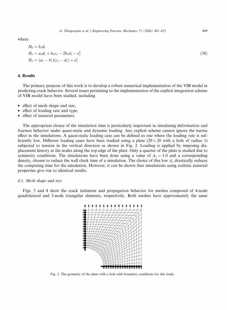
ficiently low. Different loading cases have been studied using a plate (20� 20 with a hole of radius 1)
subjected to tension in the vertical direction as shown in Fig. 2. Loading is applied by imposing dis-
placement history at the nodes along the top edge of the plate. Only a quarter of the plate is studied due to
symmetry conditions. The simulations have been done using a value of Aa ¼ 1:0 and a corresponding
density, chosen to reduce the wall clock time of a simulation. The choice of this low Aa drastically reducesthe computing time for the simulation. However, it can be shown that simulations using realistic material
properties give rise to identical results.
4.1. Mesh shape and size
Figs. 3 and 4 show the crack initiation and propagation behavior for meshes composed of 4-node
quadrilateral and 3-node triangular elements, respectively. Both meshes have approximately the same
Fig. 2. The geometry of the plate with a hole with boundary conditions for this study.
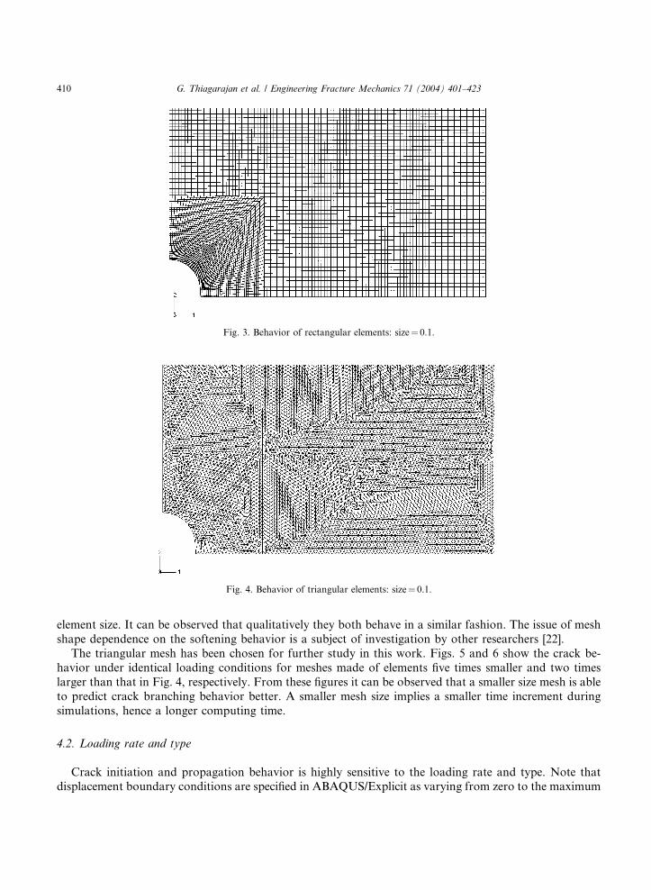
Fig. 3. Behavior of rectangular elements: size¼ 0.1.
Fig. 4. Behavior of triangular elements: size¼ 0.1.
410 G. Thiagarajan et al. / Engineering Fracture Mechanics 71 (2004) 401–423
element size. It can be observed that qualitatively they both behave in a similar fashion. The issue of mesh
shape dependence on the softening behavior is a subject of investigation by other researchers [22].
The triangular mesh has been chosen for further study in this work. Figs. 5 and 6 show the crack be-
havior under identical loading conditions for meshes made of elements five times smaller and two times
larger than that in Fig. 4, respectively. From these figures it can be observed that a smaller size mesh is able
to predict crack branching behavior better. A smaller mesh size implies a smaller time increment during
simulations, hence a longer computing time.
4.2. Loading rate and type
Crack initiation and propagation behavior is highly sensitive to the loading rate and type. Note thatdisplacement boundary conditions are specified in ABAQUS/Explicit as varying from zero to the maximum
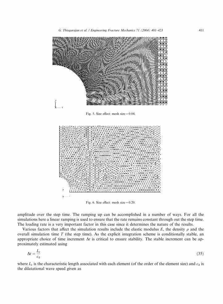
Fig. 5. Size effect: mesh size¼ 0.04.
Fig. 6. Size effect: mesh size¼ 0.20.
G. Thiagarajan et al. / Engineering Fracture Mechanics 71 (2004) 401–423 411
amplitude over the step time. The ramping up can be accomplished in a number of ways. For all the
simulations here a linear ramping is used to ensure that the rate remains constant through out the step time.
The loading rate is a very important factor in this case since it determines the nature of the results.
Various factors that affect the simulation results include the elastic modulus E, the density q and the
overall simulation time T (the step time). As the explicit integration scheme is conditionally stable, an
appropriate choice of time increment Dt is critical to ensure stability. The stable increment can be ap-
proximately estimated using
Dt ¼ Le
cdð35Þ
where Le is the characteristic length associated with each element (of the order of the element size) and cd isthe dilatational wave speed given as

Table
Crack
Den
4000
1
0.00
Cas
1
Cas
1
412 G. Thiagarajan et al. / Engineering Fracture Mechanics 71 (2004) 401–423
cd ¼
ffiffiffiffiffiffiffiffiffiffiffiffiffiffikþ 2l
q
sð36Þ
where k and l are the Lam�ee constants. Hence the number of increments (N ) required to complete the
problem can be expressed as
N ¼ TDt
¼ T1
Le
ffiffiffiffiffiffiffiffiffiffiffiffiffiffikþ 2l
q
sð37Þ
Generally the step time T would directly influence the loading rate, implying that a smaller T would result in
a faster rate of loading. However, it has been found from numerical experiments that the results are
identical, in terms of the crack growth patterns, if
K ¼ffiffiffiq
p
Tð38Þ
is constant, i.e. different T values can produce identical results. Hence it is more appropriate to define the
loading rate using K. Table 1 lists the simulation results of the crack growth patterns for different K values.
A higher value of K indicates a dynamic simulation while a lower K is for a quasi-static simulation. Figs. 7–
9 show the crack propagation behaviors for three values of K. They clearly show that, at a low K value, the
simulation results in a quasi-static crack growth behavior, Fig. 7; at an intermediate K value, the simulation
results in a dynamic crack propagation with crack branching, Fig. 8; and at a high K value, the loading rate
is so high that the elastic wave does not have time to travel down the plate before failure occurs at the top,Fig. 9.
In light of this we can rewrite Eq. (37) as
N ¼ 1
K1
Le
ffiffiffiffiffiffiffiffiffiffiffiffiffiffikþ 2l
pð39Þ
From Eq. (39) it is seen that the total number of steps, hence the wall time, required to solve a problem is
dependent only on the modulus of the material and the parameter K for a given mesh size.
The above equation would suggest that using a lower material modulus would result in fewer solution
steps. In the VIB model implemented here it is possible to use scaled values of the material modulus and
density.We conducted another numerical experiment to see if the wall time depended on the absolute values of
modulus and density. The elastic modulus was scaled to a value of unity and the corresponding equivalent
density was calculated from Eq. (37) to ensure that the simulation is identical. It was observed that the wall
1
patterns for various loading rates
sity q Step time (seconds) Increment time (seconds)ffiffiffiq
p=T Comments
0.001 4� 10�6 K0 ¼ 63; 245 Observed crack pattern
1.6� 10�5 7� 10�8 62,500 Same as above
1 5� 10�7 2� 10�9 63,245 Same as above
e when K < K0
1.0� 10�4 7� 10�8 10,000 Stable but different
crack pattern
e when K > K0
1.0� 10�5 7� 10�8 100,000 Unstable crack pattern
at top
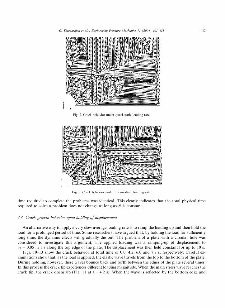
Fig. 8. Crack behavior under intermediate loading rate.
Fig. 7. Crack behavior under quasi-static loading rate.
G. Thiagarajan et al. / Engineering Fracture Mechanics 71 (2004) 401–423 413
time required to complete the problems was identical. This clearly indicates that the total physical time
required to solve a problem does not change as long as N is constant.
4.3. Crack growth behavior upon holding of displacement
An alternative way to apply a very slow average loading rate is to ramp the loading up and then hold theload for a prolonged period of time. Some researchers have argued that, by holding the load for sufficiently
long time, the dynamic effects will gradually die out. The problem of a plate with a circular hole was
considered to investigate this argument. The applied loading was a ramping-up of displacement to
u2 ¼ 0:05 in 1 s along the top edge of the plate. The displacement was then held constant for up to 10 s.
Figs. 10–13 show the crack behavior at total time of 0.0, 4.2, 6.0 and 7.8 s, respectively. Careful ex-
aminations show that, as the load is applied, the elastic wave travels from the top to the bottom of the plate.
During holding, however, these waves bounce back and forth between the edges of the plate several times.
In this process the crack tip experiences different loading magnitude. When the main stress wave reaches thecrack tip, the crack opens up (Fig. 11 at t ¼ 4:2 s). When the wave is reflected by the bottom edge and
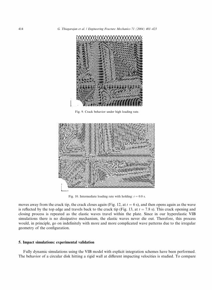
Fig. 9. Crack behavior under high loading rate.
Fig. 10. Intermediate loading rate with holding: t ¼ 0:0 s.
414 G. Thiagarajan et al. / Engineering Fracture Mechanics 71 (2004) 401–423
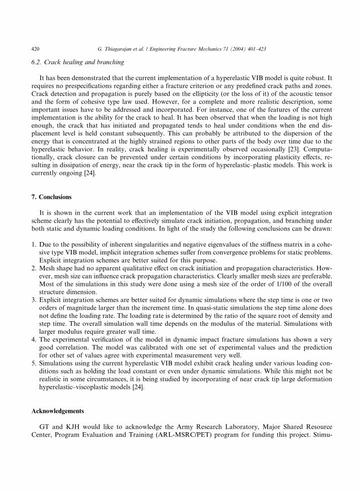
moves away from the crack tip, the crack closes again (Fig. 12, at t ¼ 6 s), and then opens again as the wave
is reflected by the top edge and travels back to the crack tip (Fig. 13, at t ¼ 7:8 s). This crack opening and
closing process is repeated as the elastic waves travel within the plate. Since in our hyperelastic VIBsimulations there is no dissipative mechanism, the elastic waves never die out. Therefore, this process
would, in principle, go on indefinitely with more and more complicated wave patterns due to the irregular
geometry of the configuration.
5. Impact simulations: experimental validation
Fully dynamic simulations using the VIB model with explicit integration schemes have been performed.The behavior of a circular disk hitting a rigid wall at different impacting velocities is studied. To compare
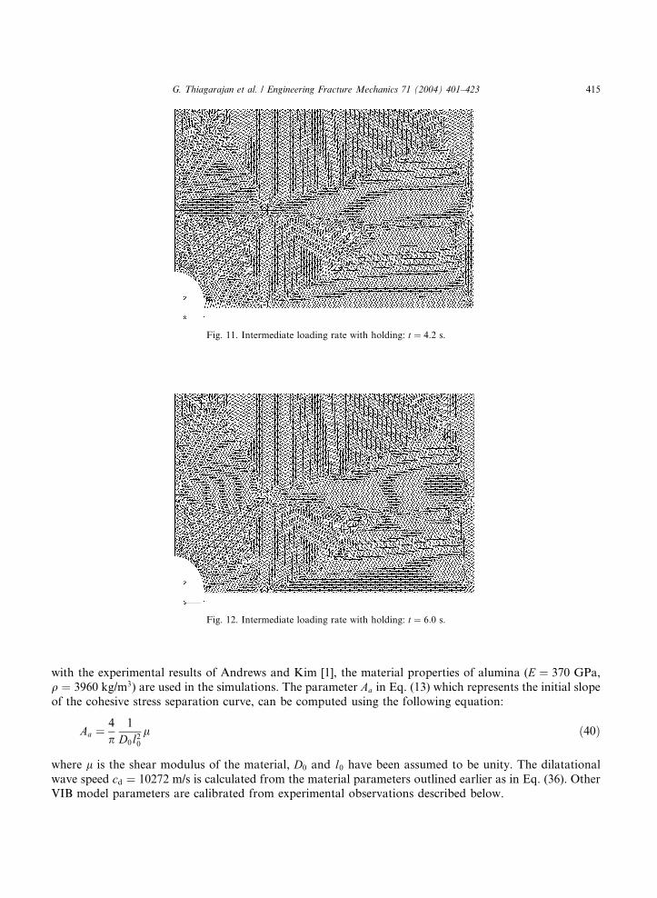
Fig. 11. Intermediate loading rate with holding: t ¼ 4:2 s.
Fig. 12. Intermediate loading rate with holding: t ¼ 6:0 s.
G. Thiagarajan et al. / Engineering Fracture Mechanics 71 (2004) 401–423 415
with the experimental results of Andrews and Kim [1], the material properties of alumina (E ¼ 370 GPa,
q ¼ 3960 kg/m3) are used in the simulations. The parameter Aa in Eq. (13) which represents the initial slope
of the cohesive stress separation curve, can be computed using the following equation:
Aa ¼4
p1
D0l20l ð40Þ
where l is the shear modulus of the material, D0 and l0 have been assumed to be unity. The dilatational
wave speed cd ¼ 10272 m/s is calculated from the material parameters outlined earlier as in Eq. (36). OtherVIB model parameters are calibrated from experimental observations described below.

Fig. 13. Intermediate loading rate with holding: t ¼ 7:8 s.
416 G. Thiagarajan et al. / Engineering Fracture Mechanics 71 (2004) 401–423
5.1. Experimental observations
Andrews and Kim [1] have studied dynamic fracture and fragmentation in brittle materials under impact
loading. They conducted tests on small, spherical alumina balls impacting a rigid anvil. Five different ball
diameters (0.4, 0.795, 1.59, 3.18 and 6.35 mm) were tested to investigate the effect of particle size on the
fragmentation process. These balls were impacted at different velocities against the anvil. Two observationsrelevant to this work are made from their data (Fig. 5 in [1]). The first is that the threshold velocity (defined
as the lowest velocity at which a ball rebounds with damage) decreases as the ball size increases from 0.40 to
3.18 mm. Secondly, the threshold velocity appears to remain relatively constant as the ball size doubles
from 3.18 to 6.35 mm.
5.2. VIB model calibration
To calibrate the VIB model, we use one set of data (0.795 mm ball diameter) from Andrews and Kim�s [1]experimental measurement to determine the parameters Aa and Bb. Once the values of Aa and Bb are de-
termined, the same values are used throughout the rest of the simulations. The value of Aa is computed as
outlined in Eq. (40). The parameter Bb (which represents the strain at which the maximum cohesive stress is
reached) was determined by matching the threshold velocity of 50 m/s reported in Andrews and Kim [1]. A
finite element mesh with 3-node plane stress triangular elements was used for the alumina disk. The anvil
was modeled using rigid link elements. The disk had 276 nodes and 500 elements. A velocity initial con-
dition was specified for the disk and simulations were run with different values of the parameter Bb. Anadvantage of studying alumina is that it has a Poisson�s ratio of 0.25. The VIB model, due to the Cauchy
symmetry properties, is ideally suited for materials with a Poisson�s ratio of 0.25.
It was found from our simulations that a value of Bb in the range of 0.0015–0.0025 resulted in the
threshold velocity of 50 m/s. Figs. 14 and 15 show the crack patterns in the disk immediately after bouncing
back for Bb values of 0.0015 and 0.0025, respectively. Values of Bb greater than 0.0025 did not result in
fracture at 50 m/s.
The simulation result with a value of Bb ¼ 0:0015 in Fig. 14 shows multiple cracks immediately after
bouncing back, while the result in Fig. 15 with Bb ¼ 0:0025 shows one single crack just appearing. Hence avalue of Bb ¼ 0:0025 was chosen for subsequent simulations for disks of different diameters. It is interesting

Fig. 14. Deformed shape of 0.795 mm disk for Bb ¼ 0:0015, v ¼ 50 m/s.
Fig. 15. Deformed shape of 0.795 mm disk for Bb ¼ 0:0025, v ¼ 50 m/s.
G. Thiagarajan et al. / Engineering Fracture Mechanics 71 (2004) 401–423 417
to note that this range of Bb, representing the strains at which brittle materials fracture, is indeed consistentwith experimentally observed fracture strain in many brittle materials such as alumina.
To simulate dynamic fracture and fragmentation behavior realistically, it is important to calibrate the
material parameters accurately, especially Bb. In the current work, Bb is calibrated using the experimental
data on critical velocity in alumina balls by Andrews and Kim [1] for one ball diameter, and the behavior
for balls with several other diameters were simulated. In principle, the value of Bb can be calibrated using an
entirely different set of experiments, e.g., quasi-static fracture and use the value to simulate dynamic
fracture cases. However, since Bb represents the strain at fracture in a brittle material, the value of Bb is
expected to be close to the value (0.0025) used in the current simulations.
5.3. Comparison with experiment
To validate of the VIB model, simulations were run for the other three diameters (1.59, 3.18 and 6.35
mm). Numerical simulations were also done for a 4 mm diameter disk. The same values of Aa and Bb as
those determined in Section 5.2 were used in these simulations. The behavior of the disk at different impact
velocities was simulated. The threshold velocity at which the disk just starts to fracture upon rebounding is
determined.
Table 2 shows a summary of the trials for disks of different diameters. The table depicts the impact
velocity, the maximum logarithmic strain in the direction normal to the fracture plane just after impact, and
the results on whether a crack has been formed. From these data the inferences of the critical impact ve-locity are done.

Table 2
Numerical observations to determine threshold impact velocity
Diameter of disk (mm) Impact velocity (m/s) Logarithmic strain (max LEyy) Conclusion
1.59 35 No crack
37 No crack
39 0.0014 No crack
41 0.1 Big center cracks
4.0 23 No crack
25 0.04 No crack
29 0.09 One central crack––small
33 0.14 One central crack––small
6.375 23 0.0013 No crack
25 0.116 Minor central crack
27 0.12 Central crack
Fig. 16. Experimental and numerical threshold impact velocities for Bb ¼ 0:0025.
418 G. Thiagarajan et al. / Engineering Fracture Mechanics 71 (2004) 401–423
Fig. 16 shows the threshold velocity as a function of ball or disk diameter from both experimental data
[1] and the VIB model simulations. It is clear that, using the model parameters calibrated from the result of
one particular ball diameter (0.79 mm), the trend of the threshold velocity versus ball diameter observed inAndrews and Kim�s [1] experiment is well captured by our simulations. Considering the fact that we
simulated circular disks as an approximation to spherical balls, the agreement between our simulation
results and that of the experiment is very good.
6. Discussions
6.1. Crack tip location
As outlined in Section 2.4 the location of the crack tip can be identified as the element in which the
acoustic tensor has last lost its ellipticity. In order to study this, a smaller tension problem was simulated.
Fig. 17 shows the deformed shape of the plate with a hole loaded in the vertical direction.

Fig. 17. Element numbers and crack path for acoustic tensor analysis.
G. Thiagarajan et al. / Engineering Fracture Mechanics 71 (2004) 401–423 419
The following observations are made:
1. While Fig. 17 clearly shows a definite crack, the propagation of the crack through the elements does not
follow a narrow crack-like path. Fig. 17 shows the sequence of elements in which the loss of ellipticity
occurred successively, which indicates that the simulated crack propagation occurs within a band of ele-
ments rather than along a single array of elements. This implies that there is loss of cohesion in the ele-
ments adjacent to the primary crack path before the crack itself opens up.2. The simulation also revealed that, while the strain at which the maximum cohesive stress is reached was
specified as Bb ¼ 0:02, the loss of ellipticity for all the elements occurred in the range of E22 ¼ 0:026–0.04.This indicates that, in the simulations, the loss of ellipticity occurs at a point beyond the plateau of the
cohesive stress–strain curve.
3. In the deformed configuration, the strains along the band of the crack path (Fig. 17) are in the range of
0.1 or more.
While it is difficult to draw definitive conclusions from this one simulation, it can be seen that there is abroad region of damage in the cohesive zone around the crack propagation path.
420 G. Thiagarajan et al. / Engineering Fracture Mechanics 71 (2004) 401–423
6.2. Crack healing and branching
It has been demonstrated that the current implementation of a hyperelastic VIB model is quite robust. It
requires no prespecifications regarding either a fracture criterion or any predefined crack paths and zones.Crack detection and propagation is purely based on the ellipticity (or the loss of it) of the acoustic tensor
and the form of cohesive type law used. However, for a complete and more realistic description, some
important issues have to be addressed and incorporated. For instance, one of the features of the current
implementation is the ability for the crack to heal. It has been observed that when the loading is not high
enough, the crack that has initiated and propagated tends to heal under conditions when the end dis-
placement level is held constant subsequently. This can probably be attributed to the dispersion of the
energy that is concentrated at the highly strained regions to other parts of the body over time due to the
hyperelastic behavior. In reality, crack healing is experimentally observed occasionally [23]. Computa-tionally, crack closure can be prevented under certain conditions by incorporating plasticity effects, re-
sulting in dissipation of energy, near the crack tip in the form of hyperelastic–plastic models. This work is
currently ongoing [24].
7. Conclusions
It is shown in the current work that an implementation of the VIB model using explicit integration
scheme clearly has the potential to effectively simulate crack initiation, propagation, and branching underboth static and dynamic loading conditions. In light of the study the following conclusions can be drawn:
1. Due to the possibility of inherent singularities and negative eigenvalues of the stiffness matrix in a cohe-
sive type VIB model, implicit integration schemes suffer from convergence problems for static problems.
Explicit integration schemes are better suited for this purpose.
2. Mesh shape had no apparent qualitative effect on crack initiation and propagation characteristics. How-
ever, mesh size can influence crack propagation characteristics. Clearly smaller mesh sizes are preferable.
Most of the simulations in this study were done using a mesh size of the order of 1/100 of the overallstructure dimension.
3. Explicit integration schemes are better suited for dynamic simulations where the step time is one or two
orders of magnitude larger than the increment time. In quasi-static simulations the step time alone does
not define the loading rate. The loading rate is determined by the ratio of the square root of density and
step time. The overall simulation wall time depends on the modulus of the material. Simulations with
larger modulus require greater wall time.
4. The experimental verification of the model in dynamic impact fracture simulations has shown a very
good correlation. The model was calibrated with one set of experimental values and the predictionfor other set of values agree with experimental measurement very well.
5. Simulations using the current hyperelastic VIB model exhibit crack healing under various loading con-
ditions such as holding the load constant or even under dynamic simulations. While this might not be
realistic in some circumstances, it is being studied by incorporating of near crack tip large deformation
hyperelastic–viscoplastic models [24].
Acknowledgements
GT and KJH would like to acknowledge the Army Research Laboratory, Major Shared ResourceCenter, Program Evaluation and Training (ARL-MSRC/PET) program for funding this project. Stimu-
G. Thiagarajan et al. / Engineering Fracture Mechanics 71 (2004) 401–423 421
lating discussions with Dr. William Walters of the Army Research Labs, Aberdeen, MD are gratefully
acknowledged. The authors would also like to thank Dr. P. Zhang for providing the UMAT subroutine of
ABAQUS finite element program for the implicit integration scheme of the VIB model. YH acknowledges
the support from the Office of Naval Research (grant #N00014-01-1-0205, program monitor Dr. Y.D.S.Rajapakse) and from National Science Foundation (grant #9983779). This work was partly supported by
National Computational Science Alliance (NCSA) under grant number OND and utilized the SGI Origin
2000 system.
Appendix A
This section outlines the details of the explicit forms of the second Piola–Kirchoff stress tensor. The basic
expression of this stress tensor is given as
SIJ ¼owoEIJ
¼ l20U0ðlÞl
nInJ
� �
Knowing that n1 ¼ sin h cos/, n2 ¼ sin h sin/, n3 ¼ cos h, and the averaging scheme is given as
h� � �i ¼Z 2p
0
Z p
0
� � �Dðh;/Þ sin hdhd/
we have
S11 ¼l20U
0ðlÞl
sin3 h cos2 /
� �
S12 ¼l20U
0ðlÞl
sin3 h sin/ cos/
� �
S13 ¼l20U
0ðlÞl
sin2 h cos h cos/
� �
S22 ¼l20U
0ðlÞl
sin3 h sin2 /
� �
S23 ¼l20U
0ðlÞl
sin2 h cos h sin/
� �
S33 ¼l20U
0ðlÞl
sin h cos2 h
� �
Appendix B. Material tangent modulus components
The components of the material tangent modulus can be expressed as shown below
AIJKL ¼ow
oEIJoEKL¼ l40
U 00ðlÞl2
��� U 0ðlÞ
l3
�nInJnKnL
�
Denoting
Aa ¼ l40U 00ðlÞl2
�� U 0ðlÞ
l3
�
422 G. Thiagarajan et al. / Engineering Fracture Mechanics 71 (2004) 401–423
we get
A11 ¼ hAa sin5 h cos4 /i
A12 ¼ hAa sin5 h cos2 / sin2 /i
A13 ¼ hAa sin3 h cos2 h cos2 /i
A14 ¼ hAa sin5 h cos3 h sin/i
A15 ¼ hAa sin4 h cos h cos3 /i
A16 ¼ hAa sin4 h cos2 / sin/ cos hi
A22 ¼ hAa sin5 h sin4 /i
A23 ¼ hAa sin3 h cos2 h sin2 /i
A24 ¼ hAa sin5 h sin3 / cos/i
A25 ¼ hAa sin4 h cos h sin2 / cos/i
A26 ¼ hAa sin4 h cos h sin3 /i
A33 ¼ hAa cos4 h sin hi
A34 ¼ hAa sin3 h cos2 h sin/ cos/i
A35 ¼ hAa sin2 h cos3 h cos/i
A36 ¼ hAa sin2 h cos3 h sin/i
Appendix C. Implicit integration scheme
The implicit integration scheme has been implemented using the subroutine UMAT by Zhang et al. [18].
The input from ABAQUS main program provides information regarding the deformation gradient and
other state variables at the current level. Using this information the constitutive theory is derived to obtain
the incremental modulus (the Jacobian) and hence an updated stress state, as follows.
The Kirchoff stress is defined as s ¼ Jr, where r is the Cauchy stress and J is the ratio of the volumes in
the final and initial configurations. The rate of Kirchoff stress can be expressed as
dsdt
¼ sOJ þ ðX � sþ s �XTÞ
where X is the spin tensor. The Jaumann rate of Kirchoff stress is defined from the constitutive theory as
sOJ ¼ M : D
where D ¼ symmðLÞ is the rate of deformation tensor, and is the symmetric part of the velocity gradient L.
The velocity gradient is given as L ¼ ov=ox where v is the velocity field. The incremental modulus matrix is
then M=J .The material rate of the second Piola–Kirchoff stress tensor is related to the rate of Green–Lagrange
strain tensor as follows:
_SS ¼ CPK : _EE
and the rate of Green strain tensor is related to D by the following equation:
_EE ¼ FT �D � F
G. Thiagarajan et al. / Engineering Fracture Mechanics 71 (2004) 401–423 423
Knowing the relationship between the Cauchy stress and second Piola–Kirchoff stress as
Jr ¼ FT � S � F
it can be shown from a detailed derivation that
sOJ ¼ D � sþ s �DT þ FT � ðCPK � FT �D � FÞ � F
where CPK is a material elasticity tensor and is the same as the material modulus tensor A shown in Eq. (9).
The above equation can then be expanded in component form to derive the incremental moduli for the
solution.
References
[1] Andrews EW, Kim KS. Threshold conditions for dynamic fragmentation of ceramic particles. Mech Mater 1998;29:161–80.
[2] Barenblatt GI. The formation of equilibrium cracks during brittle fracture: general ideas and hypotheses, axially symmetric cracks.
Appl Math Mech (PMM) 1959;23:622–36.
[3] Dugdale DS. Yielding of steel sheets containing slits. J Mech Phys Solids 1960;8:100–8.
[4] Willis JR. A comparison of the fracture criteria of Griffith and Barenblatt. J Mech Phys Solids 1967;15:151–62.
[5] Needleman A. A continuum model for void nucleation by inclusion debonding. J Appl Mech 1987;54:525–31.
[6] Larsson R. A generalized fictitious crack model based on plastic localization and discontinuous approximation. Int J Numer Meth
Engng 1995;38:3167–88.
[7] Xia L, Shih FC. Ductile crack growth––I. A numerical study using computational cells with microstructurally based length scales.
J Mech Phys Solids 1995;43:233–59.
[8] Camacho GT, Ortiz M. Computational modeling of impact damage in brittle materials. Int J Solids Struct 1996;33:2899–938.
[9] Xu XP, Needleman A. Numerical simulation of fast crack growth in brittle solids. J Mech Phys Solids 1994;42(9):1397–434.
[10] Tvergaard V, Hutchinson JW. The relation between crack growth resistance and fracture process parameters in elastic–plastic
solids. J Mech Phys Solids 1992;41:1377–97.
[11] Tvergaard V, Hutchinson JW. The influence of plasticity on mixed mode interface toughness. J Mech Phys Solids 1993;41:1119–
35.
[12] Gullerud A, Dodds R. 3-D modelling of ductile crack growth in thin sheet metals. Engng Fract Mech 1999;63:347–74.
[13] Foulk JW, Allen DH, Helms KLE. Formulation of a three dimensional cohesive zone model for application to a finite element
algorithm. Comput Meth Appl Mech Engng 2000;183:51–66.
[14] Gao H. A theory of local limiting speed in dynamic fracture. J Mech Phys Solids 1996;44:1453–74.
[15] Gao H. Elastic waves in a hyperelastic solid near its plane strain equibiaxial cohesive limit. Philos Mag Lett 1997;76:307–14.
[16] Gao H, Klein P. Numerical simulation of crack growth in an isotropic solid with randomized internal cohesive bonds. J Mech
Phys Solids 1998;46:187–218.
[17] Klein P, Gao H. Crack nucleation and growth as strain localization in a virtual internal bond continuum. Engng Fract Mech
1998;61:21–48.
[18] Zhang P, Klein P, Huang Y, Gao H, Wu PD. Numerical simulation of cohesive fracture by the virtual internal bond method.
Comput Model Engng Sci 2002;3:263–78.
[19] Milstein F. Review: theoretical elastic behavior at large strains. J Mater Sci 1980;15:1071–84.
[20] Tadmor EB, Ortiz M, Phillips R. Quasicontinuum analysis of defects in solids. Philos Mag A 1996;73:1529–63.
[21] Hill R. Accelerating waves in solids. J Mech Phys Solids 1962;10:1–16.
[22] Laurenco P, De Borst R, Rots J. A plane stress softening plasticity model for orthotropic materials. Int J Numer Meth Engng
1997;40:4033–57.
[23] Ferney BD, DeVary MR, Hsia KJ, Needleman A. Oscillatory crack growth in glass. Scripta Mater 1999;41:275–81.
[24] Thiagarajan G, Huang Y, Hsia KJ. Fracture simulations using an elasto-viscoplastic virtual internal bond model with finite
elements. ASME J Appl Mech, submitted for publication.