finite element approach of electronic structures
TRANSCRIPT

HAL Id: tel-00985912https://tel.archives-ouvertes.fr/tel-00985912
Submitted on 30 Apr 2014
HAL is a multi-disciplinary open accessarchive for the deposit and dissemination of sci-entific research documents, whether they are pub-lished or not. The documents may come fromteaching and research institutions in France orabroad, or from public or private research centers.
L’archive ouverte pluridisciplinaire HAL, estdestinée au dépôt et à la diffusion de documentsscientifiques de niveau recherche, publiés ou non,émanant des établissements d’enseignement et derecherche français ou étrangers, des laboratoirespublics ou privés.
Finite Element Approach of Electronic StructuresAmélie Fau
To cite this version:Amélie Fau. Finite Element Approach of Electronic Structures. Materials and structures in mechanics[physics.class-ph]. Ecole Centrale Paris, 2012. English. NNT : 2012ECAP0049. tel-00985912
Finite Element Approach
of Electronic Structures
THÈSE
présentée et soutenue publiquement le 10 décembre 2012
pour l’obtention du
Doctorat de l’École Centrale Paris
(spécialité mécanique, mécanique des matériaux)
par
Amélie Fau
sous la direction du Prof. D. Aubry
Composition du Jury
Président : Prof. P. Cortona (SPMS, École Centrale Paris)
Rapporteurs : Prof. F. Chinesta (GeM, École Centrale Nantes)
Prof. S Prudhomme (École polytechnique de Montréal)
Examinateur : Prof. D. Aubry (MSSMat, École Centrale Paris)
Laboratoire de Mécanique des Sols, Structures et Matériaux - C.N.R.S. U.M.R. 8579
2012ECAP0049


Acknowledgements
Je remercie les membres du jury pour le regard porté sur ces travaux, et pour les précieux conseils
et remarques partagés. Je remercie spécifiquement M. Pietro Cortona pour avoir accepté de
présider ce jury, M. Serge Prudhomme et M. Paco Chinesta pour avoir rapporté ce travail, et
pour l’attention et l’enthousiasme qu’il y ont apportés.
Je remercie M. Denis Aubry pour m’avoir proposé ce sujet de recherche, et pour ce qu’il m’a
appris, tant scientifiquement qu’humainement.
Je remercie l’École Centrale Paris pour la qualité de l’accueil dans sa structure, son école
doctorale pour sa vitalité et sa disponibilité, et le Département de Mécanique, pour m’avoir
offert des possibilités d’enseigner tout au long de ma thèse notamment M. D. Aubry, Mme A.-L.
Hamon et Mme A. Modaressi. Je pense aussi aux dynamiques équipes des laboratoires, tout
particulièrement à celle du laboratoire MSSMat, pour cet environnement d’effervescence scien-
tifique, de rencontres multiples et enrichissantes. Merci pour tous ces échanges et les amitiés qui
en sont nées.
Je remercie l’École Normale Supérieure de Cachan pour le support financier fourni pour mettre
en œuvre ces travaux, et l’ensemble du personnel de son Département de Génie Civil pour m’avoir
accueillie si chaleureusement et constructivement dans leur équipe.

Pour mes proches, de ma douce vallée, de la grande capitale, de souvenirs toulousains ou
de pays lointains, merci , ! Merci pour votre convivialité enjouée, votre simplicité raffinée, vos
projets débridés et toutes les couleurs des blés... C’est une joie d’inventer la route avec vous !

Contents
Introduction 1
I.1 Multi-scale arrangements in materials . . . . . . . . . . . . . . . . . . . . . . . . 1
I.2 Scale of the electrons in the mechanical behavior of materials . . . . . . . . . . . 3
I.3 How to obtain electronic information? . . . . . . . . . . . . . . . . . . . . . . . . 5
I.4 Objectives and outline of this dissertation . . . . . . . . . . . . . . . . . . . . . . 5
1 An ab initio perspective for modeling the mechanical behavior of materials 7
1.1 Interest of the nanoscale . . . . . . . . . . . . . . . . . . . . . . . . . . . . . . . . 7
1.1.1 Mechanical quantities of interest . . . . . . . . . . . . . . . . . . . . . . . 8
1.1.2 Electrical quantities of interest . . . . . . . . . . . . . . . . . . . . . . . . 9
1.2 Modelization at the nanoscale . . . . . . . . . . . . . . . . . . . . . . . . . . . . . 9
1.2.1 Quantum mechanics model . . . . . . . . . . . . . . . . . . . . . . . . . . 11
1.2.2 Classical mechanics model . . . . . . . . . . . . . . . . . . . . . . . . . . . 16
1.3 Our framework . . . . . . . . . . . . . . . . . . . . . . . . . . . . . . . . . . . . . 18
1.3.1 Stationary cases . . . . . . . . . . . . . . . . . . . . . . . . . . . . . . . . 18
1.3.2 Non-relativistic electrons . . . . . . . . . . . . . . . . . . . . . . . . . . . . 18
1.3.3 Absolute zero temperature . . . . . . . . . . . . . . . . . . . . . . . . . . . 19
1.3.4 Born-Oppenheimer’s hypothesis . . . . . . . . . . . . . . . . . . . . . . . . 20
1.3.5 Breaking down the wave function . . . . . . . . . . . . . . . . . . . . . . . 20
1.4 Methods to tackle the quantum electronic problem . . . . . . . . . . . . . . . . . 22
1.4.1 Hartree-Fock’s methods . . . . . . . . . . . . . . . . . . . . . . . . . . . . 23
1.4.2 Density functional theory . . . . . . . . . . . . . . . . . . . . . . . . . . . 23
i

ii CONTENTS
1.4.3 Quantum Monte Carlo calculations . . . . . . . . . . . . . . . . . . . . . . 26
1.5 Summary . . . . . . . . . . . . . . . . . . . . . . . . . . . . . . . . . . . . . . . . 27
2 Hartree-Fock’s models 29
2.1 State of the art . . . . . . . . . . . . . . . . . . . . . . . . . . . . . . . . . . . . . 31
2.1.1 Slater determinants . . . . . . . . . . . . . . . . . . . . . . . . . . . . . . 31
2.1.2 The post Hartree-Fock methods . . . . . . . . . . . . . . . . . . . . . . . . 32
2.1.3 A mathematical viewpoint of the Hartree-Fock’s models . . . . . . . . . . 33
2.2 The Galerkin method for Hartree-Fock models . . . . . . . . . . . . . . . . . . . . 34
2.2.1 The weak form of the Schrödinger problem . . . . . . . . . . . . . . . . . 34
2.2.2 The Galerkin approximation for the Schrödinger problem . . . . . . . . . 35
2.2.3 Weak formulation of the multiconfiguration problem . . . . . . . . . . . . 36
2.2.4 The weak form of the Hartree-Fock problem . . . . . . . . . . . . . . . . 39
2.2.5 Weak formulation of the configuration interaction problem . . . . . . . . . 43
2.3 Summary . . . . . . . . . . . . . . . . . . . . . . . . . . . . . . . . . . . . . . . . 45
3 Numerical strategy 47
3.1 State of the art . . . . . . . . . . . . . . . . . . . . . . . . . . . . . . . . . . . . . 47
3.1.1 Basis functions . . . . . . . . . . . . . . . . . . . . . . . . . . . . . . . . . 49
3.1.2 Evaluation of the different functions basis . . . . . . . . . . . . . . . . . . 52
3.1.3 The FEM in quantum mechanics . . . . . . . . . . . . . . . . . . . . . . . 54
3.2 The FEM strategy for the Hartree-Fock model . . . . . . . . . . . . . . . . . . . 56
3.2.1 Galerkin approximation . . . . . . . . . . . . . . . . . . . . . . . . . . . . 56
3.2.2 Newton method . . . . . . . . . . . . . . . . . . . . . . . . . . . . . . . . . 56
3.2.3 Artificial boundary conditions . . . . . . . . . . . . . . . . . . . . . . . . . 64
3.2.4 Mesh and adaptivity . . . . . . . . . . . . . . . . . . . . . . . . . . . . . . 66
3.2.5 Symmetry simplifications for atoms and linear molecules . . . . . . . . . . 67
3.3 Summary . . . . . . . . . . . . . . . . . . . . . . . . . . . . . . . . . . . . . . . . 71
3.4 Large scale perspectives . . . . . . . . . . . . . . . . . . . . . . . . . . . . . . . . 73
CONTENTS iii
4 Ab initio quantities of interest 77
4.1 The one-electron wave functions . . . . . . . . . . . . . . . . . . . . . . . . . . . . 77
4.1.1 Geometrical distribution of the individual wave functions . . . . . . . . . 77
4.1.2 Individual wave functions in bonds . . . . . . . . . . . . . . . . . . . . . . 81
4.2 The electronic density . . . . . . . . . . . . . . . . . . . . . . . . . . . . . . . . . 83
4.3 Prediction of molecular geometry . . . . . . . . . . . . . . . . . . . . . . . . . . . 89
4.4 Mechanical properties . . . . . . . . . . . . . . . . . . . . . . . . . . . . . . . . . 91
4.4.1 Stress computation . . . . . . . . . . . . . . . . . . . . . . . . . . . . . . . 91
4.4.2 Elasticity tensor computation . . . . . . . . . . . . . . . . . . . . . . . . . 93
4.5 Numerical results . . . . . . . . . . . . . . . . . . . . . . . . . . . . . . . . . . . . 94
4.6 Three-dimensional computations . . . . . . . . . . . . . . . . . . . . . . . . . . . 94
4.7 Summary . . . . . . . . . . . . . . . . . . . . . . . . . . . . . . . . . . . . . . . . 95
5 Error indicator for quantum mechanics quantities of interest 97
5.1 How exact are our results ? . . . . . . . . . . . . . . . . . . . . . . . . . . . . . . 97
5.1.1 Different quantities of interest . . . . . . . . . . . . . . . . . . . . . . . . . 98
5.1.2 The various origins of error . . . . . . . . . . . . . . . . . . . . . . . . . . 99
5.2 A very short overview of the state of the art . . . . . . . . . . . . . . . . . . . . . 104
5.2.1 Error estimate . . . . . . . . . . . . . . . . . . . . . . . . . . . . . . . . . 104
5.2.2 Error estimate for ab initio computations . . . . . . . . . . . . . . . . . . 105
5.3 A first investigation of error indicators with respect to mechanical and quantum
quantities of interest . . . . . . . . . . . . . . . . . . . . . . . . . . . . . . . . . . 106
5.3.1 Error indicator for the ground energy . . . . . . . . . . . . . . . . . . . . . 106
5.3.2 Error indicator for the probability of presence . . . . . . . . . . . . . . . . 109
5.3.3 Error indicator for the mechanical stresses . . . . . . . . . . . . . . . . . . 111
Conclusions and Perspectives 113
Bibliography 139

iv CONTENTS
Appendices 143
A A brief description of microscopes 143
B Periodic Table 147
C Atomic units 149
D Electron configurations of the atoms 151
E Quantum numbers 155
F The weak form of the Hartree-Fock system 157
G Setting up the Hartree-Fock system 161
H The Two-dimensional equations 165
I Magnetic properties 167
J Crystals: The Bloch theorem 169

Introduction
I.1 Multi-scale arrangements in materials
Multi-scale organization can be observed for most materials. For example, concrete is studied as
a structural beam or as a plate from an engineering point of view. At that macroscopic scale,
i.e. the length scale on which objects are of a size that is observable by the naked eye, the me-
chanical behavior of concrete is generally modeled as isotropic, continuous, and homogeneous.
Under the elasticity hypotheses, it is characterized by its Young’s modulus and its Poisson’s ra-
tio. To understand this macroscopic behavior, smaller scales can be explored. Concrete appears
to be built from aggregates surrounded by a cement paste. The material at that scale is discon-
tinuous and non homogeneous. Each constituent can be assumed as isotropic, continuous, and
homogeneous. To characterize the hydrated cement paste, we look at it from a microscopic scale.
The cement paste is composed of different constituents: calcium hydroxide CH, calcium silicate
hydrate CSH, and calcium aluminate hydrates CAH. A challenging endeavor is to describe CSH
gel [PKS+09, DvB11]. The CSH gel is made up of nuclei and electrons. The study of the nuclei
provides information on the behavior of the gel. The behavior of the nuclei themselves depends
on the interactions created by the nuclei network and the electronic cloud. The most refined
model for a mechanical description consists in looking into the behavior of the electrons.
Similarly, an alloy can be seen as a homogeneous material from an engineering point of
view, an assembly of grains at a microscopic scale, an assembly of atoms with a periodic or
quasiperiodic arrangement or as a nuclear network surrounded by an electronic cloud. As a third
example, the layered structures of a clay are detailed in Table 1.

2In
troducti
on
Homogeneous Heterogeneous Mesoscopic scales Atomic scale
Macroscopic scale
Concrete
Granulates and Ettringite (SEM) A molecular model of CSH [PKS+09]:cement paste [vHWvdK03] : oxygen, : hydrogen (water molecules),
: inter and : intra-layer calcium ions,: silicon, : oxygen (silica tetrahedra).
Alloy
Austenite grains (OM) [NMCO08] Al111 crystal (HRTEM) [RJR+07]
Clay
Kaolinite layers (SEM) A kaolinite layer (modified from [Gri62])
Table 1: Different organization scales of concrete, alloy and clay (OM: Optical Microscope, SEM: Scanning Electron Microscope,
HRTEM: High-Resolution Transmission Electron Microscope)

Introduction 3
In many application fields, such as aeronautics and civil engineering, engineers have to deal
with design problems in which the structures can be several meters large. For these problems,
only the structure is of interest, so what could motivate engineers to give a special attention on
the electronic scale?
I.2 Scale of the electrons in the mechanical behavior of materials
To study the mechanical behavior, the scales of interest are between the macroscopic scale
and the electronic scale depending on the quantity of interest. At the lowest scale, mechanical
characteristics are due to atom displacements associated with the rearrangement of electronic
density, especially the density of valence electrons that are involved in chemical bonding. Explor-
ing the intranuclear properties is not needed. Information acquired at the nanoscale is crucial for
enhancing strength and interfacial performance of materials. For example, [Tho11] shows that
the properties of functional ceramics are largely linked with the local microstructure (defects,
grain boundaries, intergranular films, or other precipitations) and with the distribution of these
microstructural entities at the mesoscopic or the macroscopic scale. Therefore, electronic studies
are useful to obtain a detailed view of classical engineering materials. In addition to these tradi-
tional purposes, electronic studies cannot be bypassed to explore new systems that are entirely
at the nanoscale.
Nowadays, miniaturization of industrial devices is an important process in manufacturing.
Micro-electro-mechanical systems (MEMS) [GD09] and nano-electro-mechanical systems (NEMS)
[DBD+00] are expected to significantly impact many areas of technology and science. For those
systems, the largest scale is the nanometric one and atomic studies are essential. DNA molecules
or nanotubes, whose nanometric structures are presented in Figure 1, are other examples of
nanostructures.
Beyond understanding the behavior of materials, nanoscience allows the creation of new ma-
terials whose characteristics are dedicated to a specific load or environment. For example, self
cleaning glass has been produced; titanium oxyde coats glass and breaks down organic and

4 Introduction
SEM image of CNT Carpet TEM image of graphene layers in CNT
Figure 1: Images of carbon nanotubes (CNT) [BMB09]
1931
Transmissionelectron
microscope
1935
Scanning
electronmicroscope
1946
Synchrocyclotron
1950
Synchrotron
1981
Scanningtunneling
microscope
1986
Atomicforce
microscope
Figure 2: Timeline of microscopy development
10−10 10−9 10−8 10−7 10−6 10−5 10−4 10−3 10−2distance (in m)
Infrared, X-ray microscopes
Atomic Force microscope
Transmission electron microscope
Scanning electron microscope
Optical microscope
Naked eye
Figure 3: Order of length observable depending on the microscope technologies [FPZ95]

Introduction 5
inorganic air polluants by photo-catalytic process [BSI11].
Despite these promising potentialities, the electronic scale has been explored only for the last
century due to the difficulties of its observation.
I.3 How to obtain electronic information?
Electronic systems can be examined by physical experiments or numerical simulations.
Atomic characteristics can be provided by physico-chemical analyses or by observations using
a microscope. Appendix A describes the different microscopy technologies invented during the
20th century (Figure 2) with increasing resolution (Figure 3). These devices allow currently the
observation of atomic structures. Unfortunately, they generally imply cost prohibitive facilities
and require a specific environment, including an air-conditioning system and a large area to
install them. They must be handled by specialized scientific experts, and the sample preparation
prior to observation is a long and strenuous task.
Numerical simulations and experiments can complement each other. Simulations are based
on quantum mechanics theory. They appear as an appealing alternative but they face strong
limitations. Because of the high amount of computer memory needed, the problems which can be
solved by simulations are still very simple systems. They are interesting for physical studies, but
too limited from a mechanical point of view. In recent years, the performance of computational
methods and tools increased dramatically, and representative electronic calculations can now be
achieved [Ced10].
I.4 Objectives and outline of this dissertation
This work deals only with numerical simulations of electronic systems. The goal is to collect
mechanical information of a material at the nanoscale. These properties of the material are
derived from the ground state of any system, i.e. the state of the material for which its energy is
the lowest. At the atomic level, this ground state is determined by the Schrödinger equation, but

6 Introduction
this problem cannot be solved exactly for most systems. We employ the Hartree-Fock methods
to simplify the problem. Here we propose to employ localized trial functions, and particularly
the finite element method, to approximate the solution. This numerical tool has been widely
used in other areas and offer ripe numerical background and tools. We provide error estimates
for different quantities of interest with respect to both modeling and numerical sources of error.
The outline of this document is as follows:
• Chapter 1 begins with a brief introduction of nanoscale potentialities and quantum theory.
Then, we expose the scope of our study. The exact quantum problem cannot be solved
even numerically. The usual methods and approximations to make this problem numerically
computable are described.
• Chapter 2 concentrates on the Hartree-Fock hypotheses we chose to approximate the prob-
lem. It is shown how the Schrödinger equation is turned into the Hartree-Fock system, and
introduces the different post-Hartree-Fock methods, which are derived from the Hartree-
Fock method to compute more accurate solutions.
• Chapter 3 begins with a review of the numerical methods proposed in the literature to
solve the Hartree-Fock system. These methods are evaluated with respect to their ability
to be coupled with larger scales models, the accuracy of their solutions, and their ability to
handle large systems. This evaluation hints at using the finite element method. The core
of this chapter deals with the details of the numerical strategy that we propose.
• Chapter 4 presents the results obtained for isolated systems: atoms and molecules. En-
ergies of the systems, equilibrium of internuclear distances, and mechanical and electrical
properties are computed.
• Chapter 5 focuses on error estimation. The results obtained in Chapter 4 are approximate
due to the approximations made to get a computable problem (detailed in Chapter 2) and
the employment of numerical tools (detailed in Chapter 3). The goal of the last chapter is
to estimate errors with respect to both model and numerical approximations.

Chapter 1
An ab initio perspective for modeling
the mechanical behavior of materials
We discuss, in this chapter, how considering the atomic scale can be relevant to study the
mechanical behavior of materials. The choice of this scale influences the selection of the models
to work with. Two major classes of models can be considered: either quantum mechanics models
or classical mechanics models. We detail the tools employed and the possibilities offered by
each class. We opt to utilize quantum models, and expose the framework of our study. The
mathematical problem modelizing the system cannot be solved exactly. A brief presentation of
the different solution methods proposed in the literature concludes this chapter.
1.1 Interest of the nanoscale
This work looks at materials from the atomic point of view. This scale allows the understanding
of the local properties which cannot be analyzed by simply studying materials at larger scales
e.g. the interfaces between two grains, or two materials, the atomic defects, etc. We see in
Table 1.1 that the atomic systems have nanometer-order sizes.

8 Chapter 1
Van der Waals radiusa of a H-atom 1, 2.10−10 m [Bon64]
Covalent radiusb of a H-atom 3, 2.10−9 m [PA08]
Length of the O-H bond in the H20 molecule 0, 957854.10−10 m [CCF+05]
Size of the elementary cell of LiH crystal 4, 0834.10−10 m [SM63]
Average grain size in a decarburized steel 2, 0.10−6 m [Jao08]
aradius of a conventional sphere modeling the atombhalf of the distance between two nuclei of identical atoms linked by a covalent bond
Table 1.1: Orders of magnitude of different electronic systems
Throughout this dissertation, we aim at characterizing the mechanical properties of materials
at the nanometer level. The size of the numerical samples are in the order of 10−8 m. At that
scale, we can investigate the distribution of nuclei and electrons but not the physical phenomena
inside the nuclei, which are beyond the scope of mechanical approaches.
Versatility is an advantage of the electronic approach. At this level, the same entities can
describe all types of materials, and a unique framework can define the different characteristics of
the material, such as mechanical behavior [NFP+11], electrical behavior [DGD02] or magnetic
behavior [LMZ91].
1.1.1 Mechanical quantities of interest
We can develop the concept of stress at the atomistic level [Wei02], and derive the mechanical
properties of a material at that scale from its total energy E [Sla24, NM85a, God88, IO99].
From uniform displacements δXNjof the nuclei initially located at XNj
, we define the homog-
enized deformation tensor of the nuclear network as:
δXNj= ε
(XNj
). (1.1)
The stress tensor σ and the elasticity tensor C can be defined as the derivative of the energy
density with respect to the deformation of the nuclear network ε at the first order and at the

An ab initio perspective for modeling the mechanical behavior of materials 9
second order [LC88, GM94], respectively:
σ =1
Ω
∂E
∂ε, (1.2)
C =1
Ω
∂2E
∂ε∂ε, (1.3)
where Ω denotes the volume associated with energy E.
Quantum mechanics provides the total energy of a system at the nanoscale. Provided one can
calculate the derivative of the energy with respect to the deformation ε and associate a volume Ω
to the energy E computed beforehand, we can derive both mechanical properties from nanoscale
calculations [NM85b, SB02, HWRV05].
1.1.2 Electrical quantities of interest
Besides mechanical properties, we can also benefit from quantum computations to estimate
electrical properties such as the dipole moment or the polarizability tensor [RMG65, JT03, AF05].
Similarly as before, these quantities can be derived from the total energy E when the electric field
is taken into account in the Schrödinger equation. The dipolar moment p and the polarizability
tensor α can be defined as the derivative of the energy with respect to the electric field Eel at
the first order and at the second order respectively:
p =∂E
∂Eel, (1.4)
α =∂2E
∂Eel∂Eel. (1.5)
Here, these material quantities are predicted by solving an atomic problem and determining the
ground state of the system, for which the energy is the lowest. They have to be seen as nanoscale
quantities because defects and mesoscale organization create some scale effects between nanoscale
and macroscale.
1.2 Modelization at the nanoscale
At the atomic scale, two kinds of models can be considered: either quantum mechanics models
or classical mechanics models.
10 Chapter 1
Nucleus
Electron
X1
X2
x1 x2
x3
x4
x5
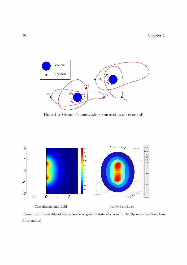
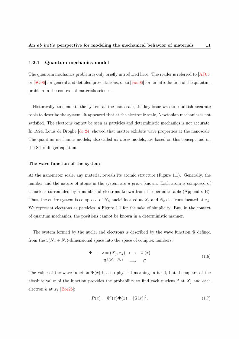
Figure 1.1: Scheme of a nanoscopic system (scale is not respected)
Two-dimensional field Isolevel surfaces
Figure 1.2: Probability of the presence of ground-state electrons in the H2 molecule (length in
Bohr radius)
An ab initio perspective for modeling the mechanical behavior of materials 11
1.2.1 Quantum mechanics model
The quantum mechanics problem is only briefly introduced here. The reader is referred to [AF05]
or [SO96] for general and detailed presentations, or to [Fou06] for an introduction of the quantum
problem in the context of materials science.
Historically, to simulate the system at the nanoscale, the key issue was to establish accurate
tools to describe the system. It appeared that at the electronic scale, Newtonian mechanics is not
satisfied. The electrons cannot be seen as particles and deterministic mechanics is not accurate.
In 1924, Louis de Broglie [de 24] showed that matter exhibits wave properties at the nanoscale.
The quantum mechanics models, also called ab initio models, are based on this concept and on
the Schrödinger equation.
The wave function of the system
At the nanometer scale, any material reveals its atomic structure (Figure 1.1). Generally, the
number and the nature of atoms in the system are a priori known. Each atom is composed of
a nucleus surrounded by a number of electrons known from the periodic table (Appendix B).
Thus, the entire system is composed of Nn nuclei located at Xj and Ne electrons located at xk.
We represent electrons as particles in Figure 1.1 for the sake of simplicity. But, in the context
of quantum mechanics, the positions cannot be known in a deterministic manner.
The system formed by the nuclei and electrons is described by the wave function Ψ defined
from the 3(Nn +Ne)-dimensional space into the space of complex numbers:
Ψ : x = (Xj , xk) 7−→ Ψ(x)
R3(Nn+Ne) −→ C.
(1.6)
The value of the wave function Ψ(x) has no physical meaning in itself, but the square of the
absolute value of the function provides the probability to find each nucleus j at Xj and each
electron k at xk [Bor26]:
P (x) = Ψ∗(x)Ψ(x) = |Ψ(x)|2, (1.7)
12 Chapter 1
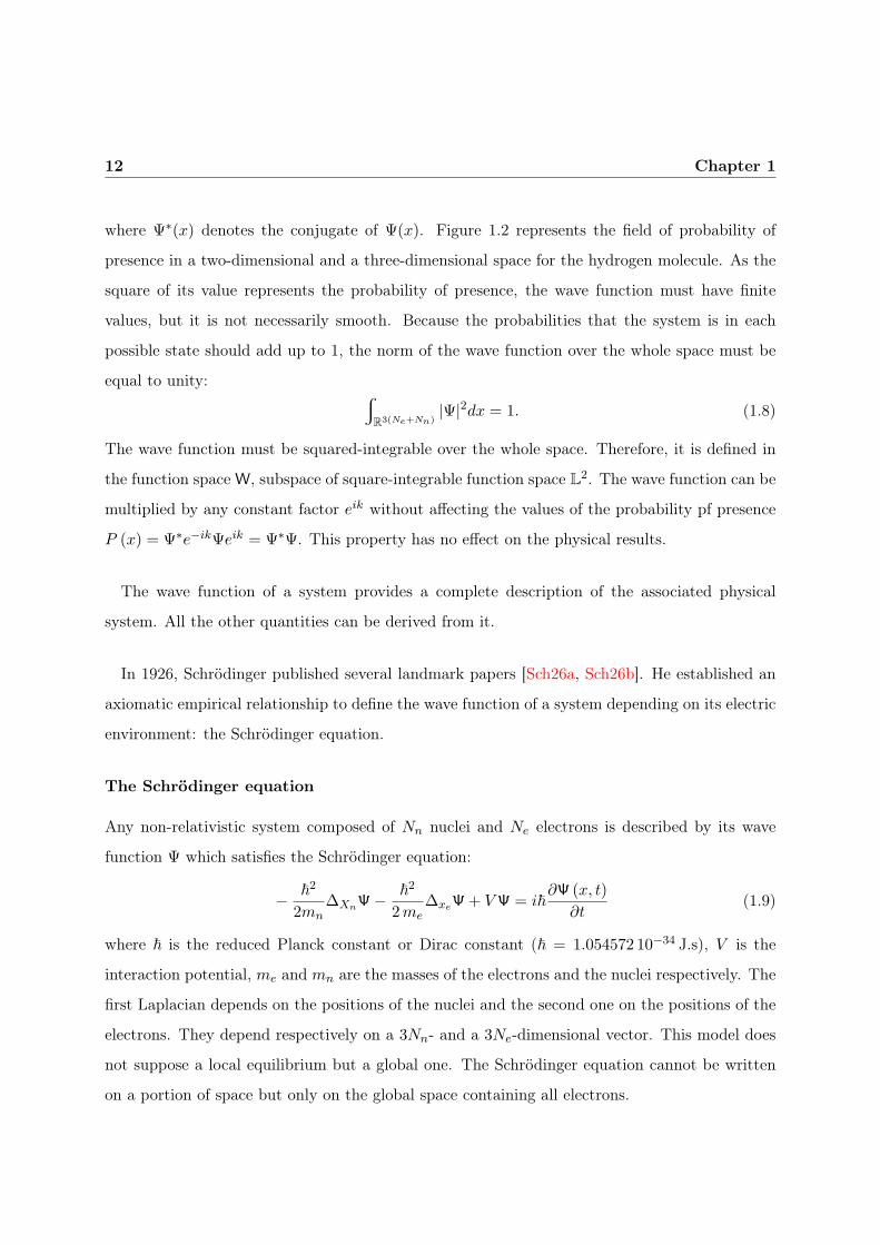
where Ψ∗(x) denotes the conjugate of Ψ(x). Figure 1.2 represents the field of probability of
presence in a two-dimensional and a three-dimensional space for the hydrogen molecule. As the
square of its value represents the probability of presence, the wave function must have finite
values, but it is not necessarily smooth. Because the probabilities that the system is in each
possible state should add up to 1, the norm of the wave function over the whole space must be
equal to unity:w
R3(Ne+Nn)|Ψ|2dx = 1. (1.8)
The wave function must be squared-integrable over the whole space. Therefore, it is defined in
the function space W, subspace of square-integrable function space L2. The wave function can be
multiplied by any constant factor eik without affecting the values of the probability pf presence
P (x) = Ψ∗e−ikΨeik = Ψ∗Ψ. This property has no effect on the physical results.
The wave function of a system provides a complete description of the associated physical
system. All the other quantities can be derived from it.
In 1926, Schrödinger published several landmark papers [Sch26a, Sch26b]. He established an
axiomatic empirical relationship to define the wave function of a system depending on its electric
environment: the Schrödinger equation.
The Schrödinger equation
Any non-relativistic system composed of Nn nuclei and Ne electrons is described by its wave
function Ψ which satisfies the Schrödinger equation:
− ~2
2mn∆XnΨ− ~
2
2me∆xeΨ+ VΨ = i~
∂Ψ (x, t)
∂t(1.9)
where ~ is the reduced Planck constant or Dirac constant (~ = 1.054572 10−34 J.s), V is the
interaction potential, me and mn are the masses of the electrons and the nuclei respectively. The
first Laplacian depends on the positions of the nuclei and the second one on the positions of the
electrons. They depend respectively on a 3Nn- and a 3Ne-dimensional vector. This model does
not suppose a local equilibrium but a global one. The Schrödinger equation cannot be written
on a portion of space but only on the global space containing all electrons.

An ab initio perspective for modeling the mechanical behavior of materials 13
For stationary cases which will be detailed in section 1.3.1, Ψ (x, t) = Ψ (x) e−E~it, the Schrödinger
equation defines the eigenpair wave function/energy of the system Ψ, E:
− ~2
2mn∆XnΨ− ~
2
2me∆xeΨ+ VΨ = EΨ. (1.10)
When using atomic units (Appendix C), the stationary Schrödinger equation reads
− me
2mn∆XnΨ− 1
2∆xeΨ+ VΨ = EΨ. (1.11)
Wave functions appear as eigenmodes of this equation. The solution is not unique. The wave
function related to the lowest energy is called the ground state. The others are called excited
states. The ground-state system is in a stationary state whereas the lifetime of excited states is
in the order of 10−10 s [FCC96].
If Ψ1 and Ψ2 are solutions of the Schrödinger equation with the same energy E, any linear
combination λ1Ψ1 + λ2Ψ2 is also a solution of this equation. The superposition principle may
be applied to the wave functions.
Potential energies
The wave function constituting a system depends on its environment, which is described by
the interaction potential energy V . It is the sum of the internal and the external interaction
potential energies. Particles inside the system determine the internal potential energy. The
external potential one is due to external particles and electric or magnetic fields.
Internal potential energy Internal potential energy can be divided into three contributions:
interactions between nuclei Vnn, between electrons and nuclei Ven, or between electrons Vee.
Nuclei are characterized by their positionXj and their atomic number Zj . Electrons are described
by their position xk. Their charge is the elementary charge e, equal to one atomic unit. For the
sake of clarity, we do not write it explicitly here, but two electrons interact only if they have the
same spin-eigenvalue.
Considering only cases when interaction potentials between particles are Coulomb potentials
[Cou84], the expressions of the different potential energies are as follow:
Vnn(Xi, Xj) =e2ZiZj
4πε0|Xi −Xj |,
14 Chapter 1
Ven(Xj , xk) =−e2Zj
4πε0|Xj − xk|,
Vee(xk, xl) =e2
4πε0|xk − xl|.
In atomic units, the internal potential energies are expressed in Hartree (1 Ha = 4.360×10⁻¹⁸ J,
see Appendix C). They are estimated by
Vnn(Xi, Xj) =ZiZj
|Xi −Xj |, (1.12)
Ven(Xj , xk) =−Zj
|Xj − xk|, (1.13)
Vee(xk, xl) =1
|xk − xl|. (1.14)
Potential energies tend to vanish when the distance between two particles tends to infinity.
Potential energy is positive when both particles have the same charge sign (repulsion), whereas
it is negative when they have opposite charges (attraction).
External potential energy The only external source studied here is the application of a
uniform external electric field Eel. V el
e is the potential energy caused by the interactions between
the external electric field and the electrons:
V ele (xk) = exk.E
el. (1.15)
V eln is the potential energy caused by the interactions between the external electric field and the
nuclei:
V eln (Xj) = eZjXj .E
el. (1.16)
In atomic units, for a uniform electric field, the expressions of the external electric field potential
energies [AF05] read
V ele (xk) = xk.E
el, (1.17)
V eln (Xj) = ZjXj .E
el. (1.18)
Non uniform fields would involve interaction with higher multipoles.

An ab initio perspective for modeling the mechanical behavior of materials 15
The magnetic potential of a system under the application of an external magnetic field B is,
similarly as before [NLK86]:
V mage (xk) = e i (∇xk
. ∧B)xk, (1.19)
V magn (Xj) = e i Zj (∇xk
. ∧B)Xj . (1.20)
These expressions evaluate the “load” borne by each particle of the system. As stated previ-
ously, the total energy is the key information to derive the mechanical properties of the material.
The total energy of the system
From (1.11), satisfying the normality condition (1.8) and using integration by parts, we get:
E =w
R3(Ne+Nn)
(
1
2
∣∣∣∣
me
mn∇xnΨ
∣∣∣∣
2
+1
2|∇xeΨ|2 + V |Ψ|2
)
dx. (1.21)
The termsrR3(Ne+Nn)
1
2
∣∣∣∣
me
mn∇xnΨ
∣∣∣∣
2
dx andrR3(Ne+Nn)
1
2|∇xeΨ|2dx represent respectively the ki-
netic energies of the nuclei and the electrons. The termrR3(Ne+Nn) V |Ψ|2dx represents the po-
tential energy.
The total energy appears as the eigenvalue of the Schrödinger equation. The spectrum of
eigenvalues can be very large. The mathematical properties of the spectrum are studied in
Section 2.1.3. Because some eigenvalues can be degenerated, the dimension of the eigenspace is
not necessarily equal to the number of eigenvalues. Hence the system is completely described by
its eigenmodes rather than by its eigenvalues.
The ground-state energy provided by these quantum models can be used to define the equi-
librium positions of the nuclei or to derive some mechanical, electrical, or magnetic properties,
as presented in section 1.1. These models provide advantageously the accurate tools to analyze
the electronic properties. Moreover, they do not need - at least theoretically - empirical param-
eters but only fundamental physical constants. Their major drawback is that they are quite
complicated numerically. Therefore, computable systems have a small number of atoms and a
small time scale. For stationary cases, simulations are limited to systems of 100 or 1000 atoms
[CLM06]. Dynamic simulations are very time consuming, and only short time scale on the order
of one picosecond (10−12 s) can be computed [CLM06].

16 Chapter 1
Real-world problems are immensely large quantum systems. Therefore, solving problems with
a quantum approach requires special strategies [You01]. An attractive alternative is to use
empirical models based on classical mechanics.
1.2.2 Classical mechanics model
The most usual empirical simulations use molecular dynamics [MH09]. The atoms are considered
as material points satisfying Newtonian mechanics [Fre71, Fey99]. Empirical potentials represent
interactions between particles. The expressions of the potentials between two electrons Vee are
established through preliminary quantum computations or experimental data. Depending on the
model refinement, the energy contribution from each pair of interacting particles is considered
as a 2-body potential:
Vee =
Ne∑
i=1
Ne∑
j=i+1
f2b (xi, xj) , (1.22)
as a 3-body potential:
Vee =
Ne∑
i=1
Ne∑
j=i+1
f2b (xi, xj) +
Ne∑
i=1
Ne∑
j=1j 6=i
Ne∑
k>j
f3b (xi, xj , xk) , (1.23)
or generally as a N-body potential. The force exerted on a given particle is given by the derivative
of the energy with respect to the position of that particle:
Fi = −Ne∑
j=1
∂
∂xif2b (xi, xj)−
Ne∑
j=1
Ne∑
k>j
∂
∂xif3b (xi, xj , xk) . (1.24)
This type of model has several drawbacks. Because it uses empirical parameters, it requires a
preliminary study of the molecules considered. Therefore, it cannot predict the behavior of new
molecular systems, either easily simulate chemical reactions, during which wave functions, and
so potentials, are largely modified. In addition, it cannot provide electronic information.
Its major advantage is that it is easier to solve numerically, allowing one to compute a large
number of atoms, up to several millions for stationary cases [CWWZ00, KOB+02, HTIF06]. This
large number of atoms or molecules can be used in the context of statistical physics.

An ab initio perspective for modeling the mechanical behavior of materials 17
To sum up, the major difference between ab initio and empirical models is that ab initio
models provide a quantum description due to the wave function of the system, whereas empirical
models provide a classical description due to the position and the velocity of the particles. The
coexistence of these two models raises two issues. The first is the compatibility between the two
modelizations, and the second is how to couple these approaches to benefit from their strong
points and minimize their shortcomings.
Ehrenfest’s theorem [NP06] states that classical mechanics equations can be derived from
quantum mechanics equations by considering particles as localized wave packets [CDL73, BD06].
This hypothesis is satisfied for most macroscopic systems. Thus, quantum mechanics can be seen
as a more general theory than classical mechanics. However quantum mechanics is quite special
because it requires some concepts of classical mechanics to express some of its principles.
From a numerical point of view, different strategies can be performed to “couple” quantum
and empirical models. Praprotnik et al. propose a solver equipped with a flexible simulation
scheme changing adaptively the model in certain regions of space on demand. Model coupling
is a very active research domain which proposes various strategies depending on the problem
characteristics. For instance, change of scale from nanoscale to macroscale can be performed by
providing information for larger scale models [PSK08], by homogenization [Le 05], by statistical
models through Boolean schemes [Mor06], or by an energetic volume coupling method such as
the Arlequin method [Ben98]. Brown et al. [BTS08] propose a “one-way coupling” of these
different models: he performs an ab initio calculation to estimate local potentials between some
molecules, and then used these potentials as input data in an empirical model. To our knowledge,
no “two-way coupling” model has been proposed in the literature until now.
To derive the mechanical properties of materials from the electronic scale, we implement a
quantum model whose framework is detailed hereafter.

18 Chapter 1
1.3 Our framework
Because the aim of this research is to collect mechanical information, we only focus on stationary
cases.
1.3.1 Stationary cases
Note that, in the context of quantum mechanics, stationary states involve wave functions de-
pending on time, but whose probability of presence is independent of time:
∂Ψ (x, t)
∂t6= 0 but
∂|Ψ (x, t) |2∂t
= 0. (1.25)
Therefore, |Ψ (x, t) |2 = |Ψ(x) |2. The general form of the wave function is Ψ (x, t) = Ψ (x) eiαt.
For stationary cases, the total energy E of the system is constant with respect to time. Therefore,
the general form of such a solution is Ψ (x, t) = Ψ (x) eiαt where α = −E~
. This dissertation
examines only the amplitude of the wave function that we also denote by Ψ.
1.3.2 Non-relativistic electrons
We suppose electrons to be non-relativistic. This assumes that the speed of electrons is largely
smaller than the speed of light, and therefore the kinetic energy of electrons is negligible compared
to the mass energy of electrons Em = mec2 (c = 299, 792.458 m.s−1).
To compute electrons of heavy atoms, and especially their core electrons whose speed is the
most important, we would have to apply relativistic models. Desclaux et al. [DDE+03] survey the
different approaches of relativistic models. The most used one is the Dirac-Fock model [IV01].
The Dirac equation [Dir28] is
(mnc
2β +mec2β − i~cγ∇Xn − i~cγ∇xe
)Ψ = i~
∂Ψ (x, t)
∂t(1.26)
where β and γ are Dirac’s matrices. For stationary cases, the equation turns into
(mnc
2β +mec2β − i~cγ∇Xn − i~cγ∇xe
)Ψ = EΨ. (1.27)
Using the Schrödinger equation, a relativistic approach has been proposed by some authors
using a pseudopotential [LCT72] or by an a posteriori perturbation [PJS94].

An ab initio perspective for modeling the mechanical behavior of materials 19
1.3.3 Absolute zero temperature
We only focus on systems at 0 K temperature, so that entropy is at a minimum. This hypothesis
assumes that the system would be fully removed from the rest of the universe, since it does not
have enough energy to transfer to other systems. At this temperature, the wave functions that
are solutions of the system are those with the lowest energy.
At a temperature different from 0 K, the system produces a thermal radiation i.e. electro-
magnetic waves [GH07]. To extend to these cases, not only the ground state must be computed
but also other states, with higher energies, called excited states. The effect of temperature is
described through a statistical distribution between these different states [Kit04, LL05]. Two
major statistical distributions are employed depending on the value of the average intermolecu-
lar distance with respect to the average de Broglie wavelength. The de Broglie wavelength λB is
the ratio between the Planck constant h and the norm of the momentum of particles p: λB =h
|p| .
If the average intermolecular distance R is smaller than the thermal de Broglie wavelength
λB, the Fermi-Dirac distribution is considered. At the absolute temperature T , the number ni
of electrons in state i, with energy Ei and degenerate degree gi, is given by:
ni =gi
exp
(Ei − µ
kBT
)
+ 1
(1.28)
where µ is the chemical potential and kB is Boltzmann’s constant.
If the average intermolecular distance R is much greater than the average thermal de Broglie
wavelength, the Maxwell-Boltzmann distribution is applied. Among the Ne electrons of the
system, the number ni of electrons in state i, with energy Ei and degenerate degree gi, is given
by the following expression:
ni = Negie
−Ei
kBT
∑Ne
j=1 gje−
EjkBT
. (1.29)
The effect of temperature is beyond the scope of this dissertation. We only compute the ground
state of the system from Equation (1.11). This equation, defined in a very large space, requires
some simplifications to be solvable for most systems.

20 Chapter 1
1.3.4 Born-Oppenheimer’s hypothesis
In the Schrödinger equation (1.11), the Laplace operators depend on the 3 (Nn +Ne)-dimensio-
nal vector x which represents the positions of all the particles in the system. The first Laplacian
depends on the positions of the nuclei and the second one on the positions of the electrons.
Each nucleus is composed of protons and neutrons. A proton and a neutron are 1836 and 1839
times heavier than an electron, respectively. Therefore, nuclei are much heavier than electrons,
between 103 and 105 times depending on the atom. The Born-Oppenheimer hypothesis [BO27]
assumes electron motion to be independent of nuclei motion. The kinetic energy of the nuclei
− me
2mn∆xnΨ can thus be omitted with respect to the kinetic energy of the electrons −1
2∆xeΨ.
The Schrödinger equation turns into:
− 1
2∆xeΨ+ VΨ = EΨ. (1.30)
Under Born-Oppenheimer’s hypothesis, the wave function is still defined in a 3 (Ne +Nn)-
dimensional space. It is only the dimension of the space of the Laplacian derivation that is
reduced.
It is common to extend this hypothesis to break the global wave function down into two
independent ones defined in smaller spaces.
1.3.5 Breaking down the wave function
We generally assume the global wave function of the system as the product of a 3Nn-dimensional
nuclear wave function Ψn and a 3Ne-dimensional electronic wave function Ψe [Thi03, CLM06]:
Ψ(Xj , xk) = Ψn(Xj)Ψe(xk), (1.31)
Ψ : R3(Ne+Nn) → C
Ψn : R3Nn → C
Ψe : R3Ne → C.
Under this assumption, these two wave functions can be solved independently. The nuclear
problem is solved using classical mechanics, whereas the electronic problem requires quantum
mechanics.

An ab initio perspective for modeling the mechanical behavior of materials 21
Nuclear problem solved by classical mechanics
The Nn nuclei are modeled by non-quantum particles characterized by their atomic number Zj .
They are described by their positionXn and not by a wave function. Each nucleus has a mass mn.
It is submitted to a force Fn derived from the nuclear Coulomb potential Vn = Vnn + Ven + V eln :
Fn = −∇XnVn = mn∂2Xn
∂t2. (1.32)
The positions Xn are estimated using classical deterministic mechanical laws, and the acceler-
ations are estimated by molecular dynamics. To determine the ground state of the system, we
minimize the energy functional of the system in which the nuclei positions appear as parameters.
The nuclear problem is a geometric optimization on R3Nn [CLM06].
Electronic wave function
The Ne electrons are elementary quantum particles. They are described by a wave function
Ψe, which obeys the following electronic Schrödinger equation (in atomic units) defined from a
3Ne-dimensional space:
HeΨe = −1
2∆xeΨe + VeΨe = EeΨe (1.33)
where Ve stands for the electronic Coulomb potential: Ve = Ven + Vee + V ele and He is the
electronic Hamiltonian operator of the system.
Let us examine the properties of the electronic wave function. From equation (1.7), we can
establish that the probability distribution of the presence of electrons is the square of the absolute
value of the electronic wave function:
Pe(xe, t) = |Ψe(xe, t)|2. (1.34)
From equation (1.8), we deduce that the electronic wave function must satisfy a normality con-
dition over the 3Ne-dimensional space:
w
R3Ne|Ψe|2dx = 1. (1.35)

22 Chapter 1
The exclusion principle, also called the Pauli principle [Pau25], states that two non-identical
electrons may not occupy the same quantum state simultaneously. To satisfy this principle, the
electronic wave function solution is chosen as an anti-symmetric function with respect to the
permutation of the positions of the electrons xi:
Ψe(xσ(1), . . . , xσ(Ne)) = sg (σ)Ψe(x1, . . . , xNe) (1.36)
where σ is a permutation on [1, Ne] and sg(σ) is its signature.
The electronic quantum problem is a partial differential equation defined in R3Ne , for which
the positions of the nuclei appear only as parameters. Considering this framework, the total
energy E of the system can be divided into a nuclear part En and an electronic one Ee:
E = En + Ee. (1.37)
Considering the kinetic energy of nuclei to be negligible with respect to the kinetic energy of
electrons, the nuclear contribution is only due to the potential energy:
En = Vnn + V eln . (1.38)
Along the same line as previously (section 1.2.1), we can express the electronic energy Ee as
Ee =w
R3Ne
(1
2|∇xeΨe|2 + (Ven + Vee + V el
e )|Ψe|2)
dx+1
2
w
∂Ωe
(∇neΨe,Ψ∗e) dx. (1.39)
Therefore, from the electronic Schrödinger equation (1.33), we can estimate the electronic wave
function but this equation can be solved analytically only for very simple cases like the hy-
drogenoid and the H+2 ions, systems with only one electron. For general systems, the equation is
defined on a highly multi-dimensional domain and cannot be easily solved, even numerically. We
briefly present in the next section the different approximations proposed to tackle this problem.
1.4 Methods to tackle the quantum electronic problem
Three major families of methods have been proposed to approximate the electronic solution:

An ab initio perspective for modeling the mechanical behavior of materials 23
• the Hartree-Fock method, where the wave function Ψe is assumed to be the product of
one-electron wave functions ϕi. It is referred to as a “rigorous energy/approximate wave
function approach” in [DL97];
• the density functional theory, which describes the system through a unique three-dimensional
electron density. It is referred to as a “rigorous density/approximate energy approach” in
[DL97];
• the Monte-Carlo method, which relies on repeated random sampling and allows for the
estimation of the high-multidimensional global wave function.
A classification of these methods and their derivatives is represented in Figure 1.3. Saad et
al. [SCS10] give a comparative overview of them.
1.4.1 Hartree-Fock’s methods
The Hartree-Fock method has been developed around 1930. Because it is generally solved using
a self-consistent algorithm, it was formerly called self-consistent field method (SCF) [SO96].
Assuming electrons are essentially independent, the form of a determinant is imposed to the
global electronic wave function [Sla29]. The resulting solutions behave as if each electron was
submitted to the mean field created by the external potential and all the other particles.
Its major drawback is that it disregards the correlation between electrons and it does not
guarantee size consistency, i.e. it does not guarantee the additivity of energies: for two non-
interacting systems A and B, the estimation of the energy of the supersystem A-B will not be
equal to the sum of the energy of A plus the energy of B taken separately. The post-Hartree-Fock
methods were proposed later to reduce these estimation errors.
The Hartree-Fock methods are detailed in Chapter 2.
1.4.2 Density functional theory
In 1964, Hohenberg and Kohn [HK64] proved that the electron density:
ρ (x) = Ne
w
R3(Ne−1)|Ψe|2 dx2 . . . dxNe (1.40)

24 Chapter 1
Schrödinger equation
Wave function methods
Monte Carlo methods
Density functional theory
Hartree-Fock
Multiconfiguration
Variational Monte CarloDiffusion Monte CarloPath integral Monte CarloAuxiliary field Monte Carlo
Thomas-Fermi
Kohn-Sham
Møller-Plessetperturbation methodsConfiguration interactionCoupled cluster
LDALSDGGAMeta GGAHybrid functionals
Figure 1.3: Classification of electronic calculation methods (inspired from [CDK+03])
LDA: Local-density approximation - LSD: Local spin density - GGA: Generalized gradient ap-
proximation

An ab initio perspective for modeling the mechanical behavior of materials 25
can thoroughly describe a system. Based on this idea, density functional theory does not evaluate
the wave function Ψe itself but the electronic density. Therefore, the first advantage of this
method is to handle a unique three-dimensional function to describe any system. It is less time-
consuming than the Hartree-Fock approach. Another great advantage of this method is that it
takes into account the correlation effects, leading to accuracy improvement.
The fundamental state is computed by minimizing the electronic energy functional EDFTe ,
which depends on the electronic density. This energy functional includes the kinetic energy of
the electrons Ec[ρ(x)], the electron-nucleus potential, possibly the potential due to an external
electric field, and the Coulomb interactions between the electrons:
EDFTe [ρ(x)] = Ec[ρ(x)] +
w
R3ρ(x)Ven(x)dx+
1
2
w
R3
w
R3
ρ(x1)ρ(x2)
|x1 − x2|dx1dx2 + Exc[ρ(x)]. (1.41)
The last term Exc[ρ(x)], called the exchange-correlation energy functional, cannot be exactly
estimated. Establishing the approximate expression of this term is the main difficulty in the
DFT method and the key to improve the accuracy of the results [RC04, TCA08b]. The simplest
approximation is the local-density approximation (LDA). It is based on the interaction energy for
a uniform electron gas. Therefore, it describes the exchange-correlation energy as an analytical
function of the electron density ρ.
Generalized gradient approximations (GGA) consist in writing the energy as a function of
the electron density ρ and the gradient ∇ρ [PBE96].
Meta GGAs methods consider dependence on ρ, ∇ρ, and higher derivatives of ρ. Becke
proposed to improve the DFT estimation by including the Hartree-Fock exchange in a DFT
exchange-correlation functional [Bec93]. Nowadays, such hybrid functionals are largely employed
[HCA12].
DFT allows the computation of large systems. Therefore, this method is intensely employed in
materials science, both fundamental and industrial research [HWC06]. Improving the accuracy
of this method requires material expertise and should be considered for each material specifically.

26 Chapter 1
1.4.3 Quantum Monte Carlo calculations
Quantum Monte Carlo calculations have been the less used until now, despite being apparently
very powerful. They are adapted to quantum problems since they offer an easy method to
integrate over highly multidimensional space. They sample statistically the integrand and average
the sampled values. They are suitable for parallel algorithms and can easily be applied to systems
containing a thousand or more electrons.
Several quantum Monte Carlo methods exist, some of them are reviewed in [AGL03]. Va-
riational Monte Carlo (VMC) and diffusion Monte Carlo (DMC) are generally the most em-
ployed [FMNR01]. They calculate the ground-state wave function of the system and are based
on a chosen trial wave function.
Based on the Schrödinger equation (1.33), VMC uses a stochastic integration method over
the 3Ne-dimensional space. Let R be a 3Ne-dimensional vector where ri is the position of the
ith electron. Any value of R is called a walker, a configuration, or a psip in the literature.
The probability density of finding the electrons in the configuration R is P (R). We define
Rm : m = 1,M as a set of independent configurations distributed according to the probability
distribution P (R). Considering the trial wave function ΨMCe , the electronic energy
EMCe =
rΨMC∗
e (x, P )HeΨMCe (x, P )dRr
ΨMC∗
e (R)ΨMCe (R)dR
(1.42)
can be estimated by the set of independent configurations through:
EMCe ≈ 1
M
M∑
m=1
ΨMC−1
e (R)HΨMCe (R). (1.43)
The accuracy of the results relies on the initial trial wave function, the probability distribution
P (R) and the number of walkers.
DMC enhances the predictions using a projection technique with a stochastic imaginary-
time evolution to improve the accuracy of the ground-state component of the starting trial wave
function.
Path integral Monte Carlo and auxiliary field Monte Carlo compute the density matrix. They
can be used to compute systems with many electrons, possibly at finite temperature.

An ab initio perspective for modeling the mechanical behavior of materials 27
1.5 Summary
In this chapter, we have presented the general framework of our study. We will only consider
stationary systems at 0 K temperature. We decompose the unique wave function of the system
into a nuclear one and an electronic one. The nuclear problem is solved through classical me-
chanics. The electronic wave function is defined in a 3Ne-dimensional space and it is estimated
using the Schrödinger equation.
This equation can be solved analytically only for very simple cases. Even numerically, it
requires a set of hypotheses to be solved for general cases. DFT methods would allow the
computation of large systems, but the establishment of accurate exchange-correlation energy
functionals requires high-level materials science background. We choose to solve it using the
Hartree-Fock approach which is detailed in Chapter 2.


Chapter 2
Hartree-Fock’s models
Chapter 1 introduced the Schrödinger model. The Schrödinger solution Ψe defined from a 3Ne-
dimensional space satisfies the following equations:
EeΨe = −1
2∆xΨe + VeΨe
Ψe(xσ(1), . . . , xσ(Ne)) = sg (σ)Ψe(x1, . . . , xNe)
rR3Ne |Ψe|2dx = 1.
(2.1)
This set of equations is defined in a high-dimensional space. This chapter concentrates on the
Hartree-Fock methods. They provide a set of hypotheses which allow the Schrödinger equation
to be solved numerically. These methods rely on a reduction of the solution space due to specific
forms of trial functions.
The ground state of the systems can be found by minimizing the energy functional defined by
Equation (1.39), by solving the strong form defined by Equation (2.1), or by solving the weak
form of the problem that will be written below. The numerical reasons to compute the solution
by the finite element method will be exposed in Chapter 3. When choosing this discretization
method, we approximate the weak form of the problem on a finite-dimensional space, which will
be described in the second part of this chapter.
30 Chapter 2
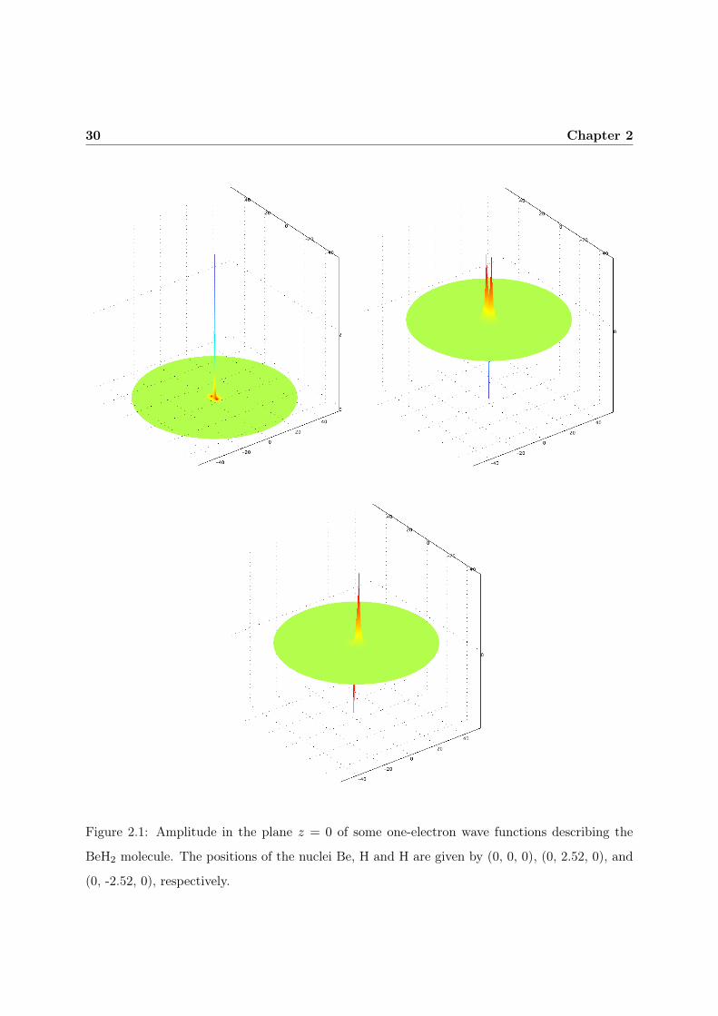
Figure 2.1: Amplitude in the plane z = 0 of some one-electron wave functions describing the
BeH2 molecule. The positions of the nuclei Be, H and H are given by (0, 0, 0), (0, 2.52, 0), and
(0, -2.52, 0), respectively.

Hartree-Fock’s models 31
2.1 State of the art
The Schrödinger solution Ψe, being an anti-symmetric function, can be expressed as an infinite
series of Ne ×Ne-dimensional determinants the so-called Slater determinants [Fri03].
2.1.1 Slater determinants
The Hartree-Fock methods approximate the Schrödinger solution by a finite series of determi-
nants, called the Slater determinants:
Ψe ∼ ΨMCe =
Nd∑
A=1
αAΨA =
Nd∑
A=1
αA√Ne!
det[
ΦA]
(2.2)
where Nd is the number of determinants involved in the series. The determinants denoted ΨA,
A = 1, . . . , Nd, are defined in R3Ne ; each determinant is built from a matrix, denoted ΦA, derived
from a vector ΦA such as:
ΨA =1√Ne!
det[
ΦA]
, ΦA(x1, . . . , xNe) =[ΦA (x1) , · · · ,ΦA (xNe)
], ΦA (x) =
ϕA1 (x)...
ϕANe
(x)
.
Each component of the vectors ΦA is defined in R3 and only depends on the coordinates of one
electron. These components are called the one-electron wave functions. Figure 2.1 illustrates
some one-electron wave functions which can be used to compute the BeH2 molecule.
For two functions a : Ω → C and b : Ω → C, we define the scalar product:
(a, b) =w
Ωa (x) b∗ (x) dx (2.3)
where b∗ is the conjugate of b. To satisfy the normality of the wave function solution defined
by equation (2.1), the determinants are normalized and the coefficients αA are computed so
that∑
A
|αA|2 = 1. The Slater determinants generally inherit normalization from the orthonor-
malization of the one-electron wave functions. The series is usually composed of determinants
that are orthogonal to each other, but some authors propose series of non-orthogonal determi-
nants [Low55].
32 Chapter 2
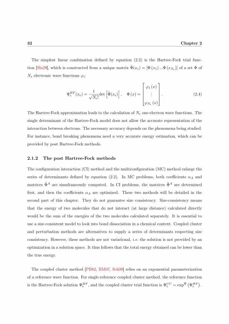
The simplest linear combination defined by equation (2.2) is the Hartree-Fock trial func-
tion [Sla29], which is constructed from a unique matrix Φ(xe) = [Φ (x1) ...Φ (xNe)] of a set Φ of
Ne electronic wave functions ϕi:
ΨHFe (xe) =
1√Ne!
det[
Φ(xe)]
, Φ (x) =
ϕ1 (x)...
ϕNe (x)
. (2.4)
The Hartree-Fock approximation leads to the calculation of Ne one-electron wave functions. The
single determinant of the Hartree-Fock model does not allow the accurate representation of the
interaction between electrons. The necessary accuracy depends on the phenomena being studied.
For instance, bond breaking phenomena need a very accurate energy estimation, which can be
provided by post Hartree-Fock methods.
2.1.2 The post Hartree-Fock methods
The configuration interaction (CI) method and the multiconfiguration (MC) method enlarge the
series of determinants defined by equation (2.2). In MC problems, both coefficients αA and
matrices ΦA are simultaneously computed. In CI problems, the matrices ΦA are determined
first, and then the coefficients αA are optimized. These two methods will be detailed in the
second part of this chapter. They do not guarantee size consistency. Size-consistency means
that the energy of two molecules that do not interact (at large distance) calculated directly
would be the sum of the energies of the two molecules calculated separately. It is essential to
use a size-consistent model to look into bond dissociation in a chemical context. Coupled cluster
and perturbation methods are alternatives to supply a series of determinants respecting size
consistency. However, these methods are not variational, i.e. the solution is not provided by an
optimization in a solution space. It thus follows that the total energy obtained can be lower than
the true energy.
The coupled cluster method [PB82, BM07, Sch09] relies on an exponential parameterization
of a reference wave function. For single-reference coupled cluster method, the reference function
is the Hartree-Fock solution ΨHFe , and the coupled cluster trial function is ΨCC
e = expT(ΨHF
e
).

Hartree-Fock’s models 33
The cluster operator T acts on the Hartree-Fock wave function to create a linear combination
of determinants with excitation rank inferior or equal to n: T = 1 +n∑
1Ti. The operator Ti
is responsible for creating all i-rank excitations. For instance, T1 =Ne∑
i=1
NV∑
j=1tji det
(
Φi,ΦjV
)
,
and T2 =Ne∑
i,j=1
NV∑
k,l=1
tklij det(
Φij ,ΦklV
)
. The exponential operator is expanded into Taylor series
eT = 1 + T +T 2
2+ ... and the coefficients t are solved through a non-linear system.
The coupled cluster method provides size extensivity of the solution, i.e. correct scaling of the
method with the number of electrons. Size consistency depends on the reference wave function.
The Hartree-Fock estimation can also be improved by the perturbation method referred by
physicists to as the Møller and Plesset method [MP34, DGG09]. The perturbed wave functions
and energies at the order k are series
Ψp =k∑
i=0λiΨi
p , Ep =k∑
i=0λiEi
p
where the Hartree-Fock
solution ΨHFe , EHF
e are considered as the zero-order perturbation Ψ0p, E
0p and λi are real
coefficients.
2.1.3 A mathematical viewpoint of the Hartree-Fock’s models
An important research activity has arisen around the existence and the uniqueness of the so-
lution for the different quantum problems. The proof of the existence of a minimizer of the
Hartree-Fock equations is presented in [LS77]. The uniqueness of the ground-state minimizer is
still an open problem [DL97]. Concerning the spectrum of solutions, Lions proved the existence
of infinitely many excited states [Lio87]. Leon also proved the existence of excited states [Leo88]
for different definitions of the excited states. One of them defines an excited state as the solution
of the minimization of the Hartree-Fock energy functional on a set of normalized Slater deter-
minant wave functions, which are orthogonal to the approximate ground state. The existence
of an energy minimum in the multiconfiguration method was established by Friesecke [Fri03].
Lewin proposed another proof for its existence, and proved the existence of saddle points for
multiconfiguration methods [Lew02, Lew04]. The application of the Hartree-Fock model for the
crystalline phase is studied in [LL05]. Despite of these numerous works, it remains a long list of
open problems [DL97].

34 Chapter 2
2.2 The Galerkin method for Hartree-Fock models
The Hartree-Fock problem can be solved either by minimizing the Hartree-Fock energy func-
tional [CH95, Szc01], by solving the associated Euler-Lagrange equations, or by solving the weak
form of the Euler-Lagrange equations. The Euler-Lagrange equations are generally favored, since
algorithms to solve them are more efficient and versatile than optimization techniques in terms of
computational effort at least when we are not too far from a solution. However, these algorithms
do not ensure convergence a priori.
The Galerkin approximation has been formulated and analyzed for density functional theory
in [LOS10]. We develop hereafter the weak form of the Hartree-Fock problems to solve them by
a Galerkin approach, which will be described and justified in Chapter 3.
2.2.1 The weak form of the Schrödinger problem
The weak form of the Schrödinger problem can be obtained by multiplying the Schrödinger
equation (eq.2.1) by the virtual term δΨe, integrating by parts the kinetic term and introducing
test multipliers with respect to the normality and anti-symmetry constraints.
Find Ψe, Ee, λσ ∈ W ×WEe ×W
λ such that:
1
2(∇xΨe,∇xδΨe) + (VeΨe, δΨe) = Ee (Ψe, δΨe) +
δEe
2[(Ψe,Ψe)− 1]
+ δλσ[Ψe(xσ(1), . . . , xσ(Ne))− sg (σ)Ψe(x1, . . . , xNe)
]
+ λσδ(Ψe(xσ(1), . . . , xσ(Ne))− sg (σ)Ψe(x1, . . . , xNe)
),
∀δΨe ∈ W, ∀δEe ∈ WEe , ∀δλσ ∈ W
λ, (2.5)
where the test Lagrange multiplier δEe is associated with the constraint ‖Ψe‖ = 1 and the test
Lagrange multiplier δλσ imposes the anti-symmetry of the approximate solution.
This equation cannot be solved exactly in general. We apply the Galerkin approach to ap-
proximate the solution.

Hartree-Fock’s models 35
2.2.2 The Galerkin approximation for the Schrödinger problem
Using the Galerkin method, the weak problem is solved in a finite-dimensional basis. The exact
solution Ψe, Ee is approximated by an eigenpair ΨG, EG where
ΨG =∑
A
αAΨA. (2.6)
The projection of the eigenfunction on each basis function is αA = (ΨG,ΨA). The normality of
ΨG is imposed through the normalization of each ΨA and a constraint on the coefficients αA.
Consequently, the problem reads:
Find ΨG, EG, µ, λσ, λAB such that:
∑
A
αA
[1
2(∇ΨA,∇δ (αBΨB)) + (VeΨA, δ (αBΨB))
]
= EG
∑
A
αA (ΨA, δ (αBΨB))
+ δµ
[∑
A
|αA|2 − 1
]
+ δλσ[ΨA(xσ(1), . . . , xσ(Ne))− sg (σ)ΨA(x1, . . . , xNe)
]
+ λσδ(ΨA(xσ(1), . . . , xσ(Ne))− sg (σ)ΨA(x1, . . . , xNe)
)
+ tr[
δλAB ·((w
ΨA ⊗Ψ∗B
)
− δABI)]
,
∀δαB ∈ Wα, ∀δΨB ∈ W, ∀δλσ ∈ W
λσ , ∀δµ ∈ Wµ, ∀δλAB ∈ W
λAB
, (2.7)
where tr denotes the trace of a square matrix and δAB is the Kronecker delta, i.e. δAB = 1 if
A = B and δAB = 0 if A 6= B. The test Lagrange multiplier δλσ imposes the anti-symmetry of
the solution, δλAB imposes the orthonormalization of the basis wave functions, and δµ constraints
the coefficients αA to satisfy∑
A
|αA|2 = 1. Now the problem can be decomposed as follows:
Find ΨA, αA, µ, λσ, λAB such that:
∑
A
αAαB
[1
2(∇ΨA,∇δΨB) + (VeΨA, δΨB)
]
+ αA
[1
2(∇ΨA,∇ΨB)X + (VeΨA,ΨB)X
]
δαB
= EG
∑
A
αAαB (ΨA, δΨB) + EG
∑
A
αA (ΨA,ΨB)X δαB + δµ
[∑
A
|αA|2 − 1
]
+ δλσ[ΨA(xσ(1), . . . , xσ(Ne))− sg (σ)ΨA(x1, . . . , xNe)
]

36 Chapter 2
+ λσδ(ΨA(xσ(1), . . . , xσ(Ne))− sg (σ)ΨA(x1, . . . , xNe)
)
+ tr[
δλAB.((w
ΨA ⊗Ψ∗B
)
− δABI)]
,
∀δΨB ∈ W, ∀δλAB ∈ WλAB
, ∀δλσ ∈ Wλσ , ∀δαB ∈ W
α, ∀δµ ∈ Wµ. (2.8)
It can be seen from (2.8) that the coefficients αA are the eigenvalues of the matrix HGABdefined
by HGAB=
[1
2(∇ΨA,∇ΨB)X + (VeΨA,ΨB)X
]
.
2.2.3 Weak formulation of the multiconfiguration problem
We consider first the MC which gives a general approach and will derive next the Hartree-Fock
(HF) and Configuration Interaction (CI) from it. The multiconfiguration model considers the
trial function ΨMCe :
ΨMCe =
Nd∑
A=1
αAΨA, (2.9)
where ΨA are determinants built from one-electron wave functions:
ΨA =1√Ne!
det[
ΦA]
. (2.10)
Consequently the constraint of anti-symmetry of the basis functions associated with the Lagrange
multipliers δλσ is satisfied. Both the set of coefficients αA and the one-electron wave functions
ΦA are computed simultaneously [WM80, MMC90].
General form of the equations system
As presented in equation (2.8), the coefficients αA are computed as eigenvalues of the matrix
HG. To guarantee a priori the orthonormality of the functions ΨA and the normality of the
solution ΨMCe , we impose through Lagrange multipliers on the one-electron wave functions:
w
R3ΦA ⊗ ΦB = δABI. (2.11)
From equation (2.8), we compute the one-electron wave functions ΦA by:
∑
A
αAαB
[1
2
(
∇detΦA,∇δdetΦB)
+(
VedetΦA, δdetΦB)]
= EG
∑
A
αAαB
(
detΦA, δdetΦB)
X

Hartree-Fock’s models 37
+ δ
[
tr
(ΛAB
2.(w
R3ΦA ⊗ ΦB − δABI
))]
. (2.12)
From elementary algebra, we can show that:
δdetΦ =
Ne∑
q=1
det (Φ (x1) , . . . , δΦ (xq) , . . . ,Φ (xNe)) . (2.13)
Because of the orthonormality of the one-electron wave functions, the products(
detΦA, δdetΦB)
vanish. Problem (2.12) can thus be reduced to:
Find ΦA,ΛAB ∈ WΦ ×W
Λ such that:
Nd∑
A=1
αAαB
[1
2
(
∇xedetΦA,∇xeδdetΦB)
xe
+(
(Ven + Vee) detΦA, δdetΦB)
xe
]
=(ΛABΦA, δΦB
)
xe
+ tr
[δΛAB
2.(w
R3ΦA ⊗ ΦB − δABI
)]
,
∀δΦB ∈ WΦ, ∀δΛAB ∈ W
Λ. (2.14)
Computations of the integrals over R3
Integrals defined on R3Ne are turned into integrals defined on R
3 due to the form of the multi-
configuration trial functions.
• First, we concentrate on the product(
∇xedetΦA,∇xeδdetΦB)
xe
. It is recast using the
one-electron wave functions as:
εiεj
[
(ϕAi1 (x1) , ϕ
Bj1 (x1)
). . .
(
∂ϕAim
(xm)
∂xm,∂δϕB
jm(xm)
∂xm
)
. . .(
ϕAiNe
(xNe)ϕBjNe
(xNe))
+(ϕAi1 (x1) , ϕ
Bj1 (x1)
). . .
(
∂ϕAim
(xm)
∂xm,∂ϕB
jm(xm)
∂xm
)
. . .
. . .(ϕAin (xn) , δϕ
Bjn (xn)
). . .(
ϕAiNe
(xNe) , ϕBjNe
(xNe))]
.
Due to the orthogonality of the one-electron wave functions, the first term of this sum va-
nishes. The second remains non zero only if A = B and ik = jk, ∀k ∈ [1;Ne]. Therefore, we
find:(
∇xedetΦA,∇xeδdetΦB)
xe
=(∇xΦ
A,∇xδΦA)
x. (2.15)

38 Chapter 2
• Secondly, we focus on the interactions between nuclei and electrons(
Ven (XM , xq) detΦA,
δdetΦB)
and write them using the one-electron wave functions:
εiεj
(
ϕAi1(x1) , ϕ
Bj1(x1)
)
. . .(
Ven (xM , xq)ϕAiq(xq) , δϕ
Bjq(xq)
)
. . .(
ϕAiNe
(xNe) , ϕBjNe
(xNe))
.
The orthonormality of the one-electron wave functions (eq. 2.11) leads to A = B, im = jm
∀m ∈ [1;Ne] and :
(
Ven (XM , xq) detΦA, δdetΦB)
=(Ven (xM , x) Φ
B, δΦB).
• Thirdly, we turn to the interactions between electrons(
Vee (xp, xq) detΦA, δdetΦB)
and
establish it can be written as:((
ΦA (xp)
|xp − xq|,ΦB (xp)
)
xp
ΦA (xq) , δΦB (xq)
)
xq
−((
ΦA (xp)
|xp − xq|⊗ ΦB (xp)
)
ΦA (xq) , δΦB (xq)
)
.
We introduce the interaction matrix GAB whose terms are:
GAB (x) =w
R3
ΦA∗
(y)⊗ ΦB(y)
|x− y| dy. (2.16)
Therefore,
(
Vee (xp, xq) detΦA, δdetΦB)
=((
tr(GAB
)I −GAB
)ΦA (xq) , δΦ
B (xq))
xq.
We note that the interaction matrix G is a convolution with a Coulomb kernel. It can be
defined as the solution of Green’s partial differential equations:
tr[
∇GAB · ∇δGABT]
= 4π tr[(
ΦA ⊗ ΦB∗)
· δGABT]
, ∀δGAB ∈ WG. (2.17)
Finally, the multiconfiguration system reads:
FindαA,Φ
A,ΛAB, GAB
such that:
∑
A
αAαB
[1
2
(∇ΦA,∇δΦB
)
x+(VenΦ
A, δΦB)
x
]
+((
tr(GAB
)I −GAB
)ΦA, δΦB
)
x

Hartree-Fock’s models 39
+ αA
[1
2(∇ΨA,∇ΨB)X + (VeΨA,ΨB)X
]
δαB − EMCe
∑
A
αA (ΨA,ΨB)X δαB
+ δµ
[∑
A
|αA|2 − 1
]
−(ΛABΦA, δΦB
)
x+ tr
[δΛAB
2.(w
R3ΦA ⊗ ΦB − δABI
)]
+ tr[
∇GAB · ∇δGABT]
− 4π tr[(
ΦA ⊗ ΦB∗)
· δGABT]
= 0,
∀δαB ∈ WΦ, ∀δΦB ∈ W
Φ, ∀δΛAB ∈ WΛ, ∀δGAB ∈ W
G, ∀δµ ∈ Wµ. (2.18)
The setδαA, δΦ
A, δΛAB, δGAB
denotes the test functions. ΛAB appears as a Lagrange
multiplier associated with the unit norm of the determinants ΨA. This system of non-
linear eigenmatrices will be solved by an iterative numerical scheme introduced in the next
chapter.
• Finally, the approximate energy for the multiconfiguration approximation is obtained as:
EMCe =
Nd∑
A=1
Nd∑
B=1
c∗AcB
(
Hedet[
ΦA (x)]
, det[
ΦB (x)])
. (2.19)
This model has also been presented in [Fri03] and in [Lew04]. It involves a very large number
of degrees of freedom and is often restricted to the Hartree-Fock trial function.
2.2.4 The weak form of the Hartree-Fock problem
We specify now the multiconfiguration formulation to Hartree-Fock as a special case. The
Hartree-Fock method considers a single Slater determinant as the trial function (see defini-
tion (2.4)). The Hartree-Fock solution ΨHFe is derived from a unique vector Φ of Ne one-electron
wave functions. Φ,Λ satisfy the following system which is derived directly from the above
multiconfiguration equations:
Find Φ,Λ such that:
1
2(∇Φ,∇δΦ) + (((Ven + tr (G)) I −G) Φ, δΦ) = (ΛΦ, δΦ) , ∀δΦ ∈ W
Φ,
tr[(I −
rR3 Φ⊗ Φ∗
)· δΛT
]= 0, ∀δΛ ∈ W
Λ,
(2.20)
where Λ appears as a matrix of Lagrange multipliers associated with the orthonormalization
of the one-electron wave functions, and δΛ as a test Lagrange-multiplier. We have to solve

40 Chapter 2
a self-consistent integro-differential system where the diagonal of the matrix Λ contains the
eigenvalues. Appendix F details how this weak form is directly established. The terms of the
interaction matrix G are:
G (x) =w
R3
Φ∗(y)⊗ Φ(y)
|x− y| dy (2.21)
that can also be defined as the solution of Laplace’s partial differential equations:
tr[∇G · ∇δGT
]= 4π tr
[(Φ⊗ Φ∗) · δGT
], ∀δG ∈ W
G. (2.22)
The Hartree-Fock strategy considers a system of Ne independent wave functions. Even if
it is only a result of the mathematical hypotheses, this approach reveals expressions of the
electronic energies. The diagonal of the matrix Λ contains the energies of the modes. They
can be linked approximately to the ionization energies by Koopman’s theorem. The accuracy of
this approximation depends on the specific system. The term 12 (∇Φ,∇Φ) represents the kinetic
energies of the wave functions. The term (VenΦ,Φ) represents the electrostatic interactions
between nuclei and electrons. Inter-electron repulsion is embedded in the term (tr (G) Φ,Φ). The
term (−GΦ,Φ) has a quantum origin: it comes from the anti-symmetry of the wave function.
The terms tr (G) and G are commonly noted J and K and are referred to as the Coulomb
operator and the exchange operator. The Hartree-Fock electronic energy reads:
EHFe =
(
−1
2∇Φ,∇Φ
)
+ Ven|Φ|2 + [tr (G) I.Φ−G.Φ]Φ. (2.23)
The strong form of the Hartree-Fock problem is classic and is obtained from the weak form (2.20)
as (see Appendix G):
−1
2∆xeΦ+ VenΦ+ [tr (G) I −G] Φ = ΛΦ
xG = −4πΦ⊗ Φ∗
rR3 Φ⊗ Φ∗ dx = I.
(2.24)
Remark: The influence of an electric potential can be incorporated into the Hartree-Fock
equation. To investigate interactions between electrons and an external electric field creating an

Hartree-Fock’s models 41
external potential energy V ele , the Hartree-Fock system reads:
(
−1
2∇Φ,∇δΦ
)
+(((
Ven + V ele + tr (G)
)I −G
)Φ, δΦ
)= (ΛΦ, δΦ) , ∀δΦ ∈ W
Φ,
tr[∇G · ∇δGT
]= tr
[(4πΦ⊗ Φ∗) · δGT
], ∀δG ∈ W
G,
tr[(I −
rR3 Φ⊗ Φ∗) · δΛT
]= 0 ∀δΛ ∈ W
Λ.
(2.25)
Remarks about spins
Two electrons interact only if they have the same spin eigenvalue. For the sake of clarity, the
spin eigenvalues are not made explicit in this dissertation, but they are taken into account in
computations. Each electronic wave function ϕi is characterized by its spin eigenvalue σi, which
can be1
2or −1
2. Since electrons are fermions, two different electrons (one with the spin eigenvalue
1
2and the other one with the spin eigenvalue −1
2) can occupy the same eigenmode. For some
systems, since all eigenmodes are occupied by two electrons, the Hartree-Fock system can be
simplified. The system of Ne electrons can be described byNe
2pairs of electrons. The Hartree-
Fock system is simplified into the Restricted Hartree-Fock (RHF) system ofNe
2components.
Systems describable by this restricted model have necessarily an even number of electrons, but
all systems with an even number of electrons cannot be described by this model, e.g. the Oxygen
atom. Electronic structures for which the Hartree-Fock system cannot be simplified must be
described by Ne wave functions and the Unrestricted Hartree-Fock (UHF) system.
Among the different eigenmodes solutions of the Hartree-Fock system, we know from the
aufbau principle that the eigenmodes which are occupied by electrons are those with the low-
est eigenvalues [AF05]. The list of occupied modes is called the electron configuration. For
our computations, the electron configuration is established using the literature. It imposes the
number of wave functions defining the system and the model describing the system, either the
restricted Hartree-Fock or the unrestricted Hartree-Fock model. Appendix D lists the electron
configurations of the isolated atoms.

42 Chapter 2
Solving the Hartree-Fock problem
Computing an arbitrary number of virtual functions
Deriving some determinants from these two sets of functions
Computing coefficients αA
Estimating the CI energy
Figure 2.2: Scheme of the configuration interaction strategy
Hartree-Fock’s models 43
Properties of the Hartree-Fock solutions
The Hartree-Fock system has symmetric properties. Let C be an orthogonal matrix, the trans-
formation Φ = CΦ transforms the system (2.24) into a system of the same form, Λ being replaced
by CΛCT . One can always find a C such that the transformed Λ becomes a diagonal matrix.
Let us examine two distinct wave functions ϕk and ϕl (with k 6= l and (k, l) ∈ [1;Ne]2),
which are assumed solutions of the Fock system (2.24). We multiply the k-th equation by ϕ∗l
and the l-th equation by ϕ∗k. Integrating over R
3 the difference of both terms and considering
the basis in which Λ is a diagonal matrix, we show that if Λkk 6= Λll, for k 6= l, then ϕk and ϕl
are necessarily orthogonal.
A way to improve the estimate of the Hartree-Fock problem without solving a problem as
complex as the multiconfiguration one is computing the configuration interaction problem.
2.2.5 Weak formulation of the configuration interaction problem
The configuration interaction approach is in fact a two-stage scheme for MC where the one-
electron wave functions are computed first as in HF, new trial waves are computed from them
and the associated αi are finally computed. The configuration interaction strategy uses the same
trial function as the multiconfiguration problem:
ΨCIe =
1√Ne!
Nd∑
A=1
αAdet[
ΦA]
. (2.26)
The one-electron wave functions ΦA are determined separately from the coefficients αA. The
coefficients αA are obtained by equation (2.8). The determination of the vectors ΦA is simplified
when compared with the multiconfiguration problem. It is divided into three steps:
• First, the Hartree-Fock problem (eq.2.20) is solved, the first vector Φ1 contains its solution.
• Then, an auxiliary vector containing any number Nv of one-electron wave functions is
computed.
• Finally, the vectors ΦA (for A ∈ ]1;Nd]) are built combining some one-electron wave
functions of Φ1 and some components of the vector ΦV .

44 Chapter 2
The one-electron wave functions ϕV i contained in the vector ΦV are called virtual wave func-
tions. The pair ΦV ,ΛV is defined as the solution of:
(
−1
2∇ΦV ,∇δΦV
)
+(((Ven + tr (G)) I −GV
)ΦV , δΦV
)=(ΛV ΦV , δΦV
), ∀δΦV ∈ W
Φ,
tr[
∇xeGV · ∇xeδG
V T]
= tr[(4πΦV ⊗ Φ∗
)· δGV T
]
, ∀δGV ∈ WG,
tr[(I −
rR3 Φ
V ⊗ ΦV ∗) · δΛV T]
= 0, ∀δΛV ∈ WΛ,
(2.27)
where ΛV appears as a Lagrange multiplier associated with the orthonormalization of the one-
electron virtual wave functions, and δΛV as a test Lagrange-multiplier. The diagonal of the
matrix ΛV contains the eigenvalues related to the electron energies of the virtual modes ϕVi . The
virtual wave funcions ϕVi are orthogonal between each other, and orthogonal to the Hartree-Fock
wave functions ϕi.
The vectors ΦA are constructed by replacing some one-electron wave functions of vector Φ by
some virtual wave functions. For instance, considering a system described by three one-electron
wave functions, three vectors ΦA can be:
Φ1 (x) =
ϕ1 (x)
ϕV1 (x)
ϕ3 (x)
, Φ2 (x) =
ϕ1 (x)
ϕV1 (x)
ϕV2 (x)
, Φ3 (x) =
ϕV2 (x)
ϕV1 (x)
ϕ3 (x)
.
Using two virtual wave functions, 18 vectors ΦA could be built: 6 vectors involve only one
virtual wave function and 12 vectors involve both virtual wave functions simultaneously. Then,
the determinants are derived from the matrices ΦA built from the vectors ΦA. The Slater
determinants constructed using k virtual wave functions are called excited states at the order k.
Since the one-electron wave functions are orthonormal, the determinants derived from these
are orthonormal. The maximum number of determinants Nd,max involved in the series depends
on the number of components of the vector Φ and on the number of virtual wave functions.
Using the maximum number of available determinants guarantees size consistency (see page 32).
The configuration interaction strategy is summed up by Figure 2.2. First, the Hartree-
Fock problem is solved, then a number of virtual functions is chosen, and these functions are

Hartree-Fock’s models 45
computed. Some determinants are derived from the wave functions contained in the vectors Φ
and ΦV . Finally, the coefficients α are computed, and the approximate energy is estimated by
equation (2.19).
2.3 Summary
In this chapter, we have presented the family of Hartree-Fock methods, also called the wave
function methods. Supposing that the wave function has the form of Slater determinants, the
Hartree-Fock strategy turns a unique equation defined from a very large space into several equa-
tions defined only from a three-dimensional space. Regrettably, it neglects electronic correlation.
The post-Hartree-Fock methods were introduced to improve results by increasing the space of
trial functions. In that case, trial functions are linear combinations of Slater determinants with
the Hartree-Fock determinant included.
The Hartree-Fock method has been used to solve quantum mechanics problems since the 1930s.
During the first decades, only small systems with very few electrons could be solved using this
method because the Hartree-Fock system is non-linear and can involve a large number of degrees
of freedom. To solve it for general cases, it requires an efficient numerical strategy. In the next
chapter, we present different numerical methods to overcome these difficulties.
The post-Hartree-Fock methods provide a hierarchy of trial functions to estimate the electronic
state of any system. Considering the hierarchy of the different solution spaces WHF ⊂ WCI ⊂ W,
the exact energy Ee is lower than the multiconfiguration energy ECIe which is lower than the
Hartree-Fock energy EHFe :
Ee 6 ECIe 6 EHF
e . (2.28)
Energy estimates become more accurate when the trial function space is enlarged. In Chap-
ter 5, we construct error estimation tools to compare the accuracy of the different trial function
spaces.


Chapter 3
Numerical strategy
In this work, we apply the Hartree-Fock and the configuration interaction methods (introduced
in Chapter 2) to approximate solutions of the Schrödinger equation. For the sake of simplicity,
the numerical strategy is presented here for the Hartree-Fock system considered as the reference
problem. The same tools and approach are used to solve the configuration interaction problem.
As discussed in the previous chapter, the Hartree-Fock problem is a non linear eigenvalue prob-
lem and involves a large number of degrees of freedom. Therefore, solving it requires powerful
numerical tools to ensure convergence, to tackle large systems and to provide accurate approx-
imations of the solutions. The first part of this chapter overviews the different strategies set
up in the literature to tackle the problem. Most involve a variational discretization based on a
finite-dimensional space of trial functions. The evaluation of the different basis sets aims at using
the finite element method to solve the Fock system. The second part of this chapter details our
finite element strategy to solve efficiently the weak form of the Fock system.
3.1 State of the art
As mentioned before, solving the Hartree-Fock problem can be done by several approaches:
minimizing the Hartree-Fock energy functional, solving the strong form of the problem, or solving
the weak form of the system. Whatever the approach, the solver requires anNb-finite-dimensional

48 Chapter 3
BeH2: ϕ1 BeH2: ϕ2 BeH2: ϕ3
H: ϕ1 H: ϕV1 Be1: ϕ1
Be1: ϕ2 Be2: ϕ1 Be2: ϕ2
Figure 3.1: Some atomic orbitals relative to the Be and the H atoms (in blue) which can be
employed as a basis set to compute the BeH2 molecule whose one-electron eigenfunctions are
represented in red. All the wave functions are represented on the axis z (i.e. x = 0, y = 0considering the following positions of the atoms: H(0;0;7.48), Be(0;0;10), and H(0;0;12.52).

Numerical strategy 49
space ν. Each wave function ϕj is expanded as a linear combination of basis functions χii∈[1;Nb]
of ν:
∀j ∈ [1;Ne], ϕj =
Nb∑
i=1
Cjiχi where Cji = (χi, ϕj)R3 . (3.1)
C is a matrix that contains the coefficients of the linear combination of χi to build ϕj .
The choice of the basis functions and their number Nb will affect the accuracy of the numerical
results. In order to optimize the convergence, Cancès et al. [CLM06] highlight the importance
of adapting the basis functions to the problem at hand. In the literature, different sets of trial
functions have been proposed.
3.1.1 Basis functions
As quantum operators are Hermitian, eigenfunctions form a basis on which all the solutions can
be developed. Using this idea, the first atomic simulations were developed on atomic orbitals
sets. Such an approach can be related to the Rayleigh-Ritz method which is very often used in
mechanics [Gou95].
Atomic orbitals
Atomic orbitals χa are eigenfunctions of isolated atoms. Figure 3.1 shows a set of atomic orbitals
relative to the Be and the H atoms which can be used as a basis set to compute the BeH2 molecule.
These trial functions are centered on each nucleus, and their number Nb is greater or equal to
the number of fundamental wave functions for the isolated atoms considered. In addition to the
atomic orbitals centered on real atoms, some authors introduce ghost atoms and ghost atomic
orbitals to enlarge the discretization basis [OM76].
Atomic orbitals can be described by different mathematical functions, such as hydrogen-like
atomic orbitals, Gaussian orbitals or Slater-type orbitals, which are detailed below.
For molecular or crystal simulations, atomic orbitals can be employed as a basis set to build
molecular orbitals [Hal91]. The Linear Combination of Atomic Orbitals (LCAO) method defines
molecular orbitals χmol as:

50 Chapter 3
χmol =∑
a
Ciaχa. (3.2)
The coefficients Cia of the linear combination are determined by a variational approach [SO96,
AF05].
In the following paragraphs, we list some mathematical functions proposed in the literature to
approximate atomic orbitals.
Slater-type orbitals In 1930, Slater introduced Slater-type orbitals, also called STOs [Sla30,
Sla32]. They are generally divided in a radial and an angular part expressed in cylindrical
coordinates (r, θ, ϕ). These two parts are independent, and are solved separately.
The angular part is usually the real part of spherical harmonics Y ml . The radial part χr
STO
is assumed to decay exponentially at long range, and has the following form:
χSTO (r) = CSTO|r|n−1e−ζ|r| (3.3)
where CSTO is a normalization constant, and n is the principal quantum number defined in the
brief introduction to quantum numbers in Appendix E. Models for atoms and molecules allow
the determination of the effective nuclear charge ζ [OPNZ00].
For example, Crystal [Cry11] is a commercial software that provides the solution of the
Hartree-Fock system using a basis of Slater-type orbitals.
Gaussian functions In 1950, Boys [Boy50] proposed Gaussian functions as atomic orbitals.
They can be called Gaussian orbitals, Gaussian type orbitals or GTOs. Alike STOs, they are
divided into independent radial and angular parts and the real part of the spherical harmonics
is used as the angular part. The radial part has the following form:
χGTO (r) = CGrle−αr2 (3.4)
where CG is a normalization constant, and l is the angular quantum number (defined in Ap-
pendix E).
Crystal [Cry11], Jaguar [Sch11] and Gaussian [Gau11] are examples of software that solve
the Hartree-Fock system with a Gaussian basis.

Numerical strategy 51
Without using atomic orbitals i.e. eigensolutions of atomic problems, trial functions can also
be mathematical constructs suitable for the Hartree-Fock simulations.
Plane or spherical waves
The electronic problem can be expanded on an orthonormal basis of plane waves [dLPZ79]. The
basis functions χPW are expressed as a function of the Cartesian coordinate x in case of plane
waves:
χPW (x) =∑
k
ckeikx (3.5)
where ck are normalization constants. Spherical waves are functions of the distance r between
the electron and the nucleus:
χSW (r) =∑
k
ckeikr. (3.6)
For localized systems, such as the first row elements or transition metals, where the vacuum area
can be large, this method generally requires a large number of basis functions. To solve this
problem, some authors propose to employ adaptive coordinates. General curvilinear coordinates
are arranged in order to be dense where the wave functions are localized [DCAJ94].
The software VASP [VAS11] is equipped with such a basis set.
Wavelets
Some authors [CAJL93] suggest a basis of wavelets. These oscillations provide an orthonormal
basis with respect to the inner product defined by eq.(2.3), localized in both real and Fourier
spaces [Cha05].
DFT++ [Cor11], MADNESS [Com11] or BigDFT [Eur11] can solve the electronic problem
with wavelets basis.
Finite element basis functions
The finite element method (FEM) provides another approach to build a basis of localized trial
functions. This discrete numerical method is widespread in the contexts of structural mechanics,
fluid mechanics, acoustics, among other domains in which partial differential equations need to

52 Chapter 3
be solved. Approximate solutions are found from discretization of the weak form of the problem.
This method is detailed in [ZT05] or in [Joh09].
The domain Ω of the FEM is segmented into M tetrahedra (in 3D). Polynomials ωpj of order
p are defined on each tetrahedron j. They constitute a basis of local functions, continuous on Ω.
Numerical solutions ϕpi , approximation of the exact solutions ϕi, are estimated on this partition
ωpj , j ∈ [1,M ]
:
ϕi ≈ ϕpi =
M∑
j=1
Cij ωpj . (3.7)
0
j − 1 j j + 1
1
Figure 3.2: A FEM basis function: ω1j of order 1
We use Lagrangian finite elements. Each polynomial takes the value 1 only at a certain
node and all the other basis functions vanish for the considered node. Therefore, approximate
functions are continuous piecewise polynomials on subdomains called “finite elements”. The
coefficients Cij are the values of the approximate wave functions ϕi at the corresponding nodes.
They are estimated numerically applying the Galerkin method to the weak form of the Hartree-
Fock electronic problem presented in Chapter 2. The quality of finite element approximations
depends on the form and the density of the mesh involved.
3.1.2 Evaluation of the different functions basis
Tsuchida and Tsukada [TT98] list the properties required for an ideal basis set: simplicity,
sparsity, high parallelizability, possibility to use non-periodic boundary conditions, possibility to
expand wave functions in real space efficiently, with non-uniformity, with computational effort
scaling linearly with the number of variables.
Numerical strategy 53
First, let us compare the different atomic orbitals between them. The general form of the
Gaussian functions is not as accurate as the form of Slater-type orbitals. Therefore, they gen-
erally require a larger number of basis functions and are not widely used for atomic or crystal
computations.
For molecular cases, a drawback of Slater-type orbitals is the fact that products of two Slater-
type orbitals of distinct atoms are difficult to compute. Gaussian orbitals are preferred because
the product of two Gaussian functions centered on different atoms can be expressed as a Gaussian
function centered on a point along the axis connecting the two atoms.
Now, let us compare atomic orbitals with other basis functions. Any kind of atomic or mo-
lecular orbitals is disadvantageous because it needs preliminary knowledge of the expressions of
atomic orbitals, specific to the atoms considered. Moreover, any atomic orbital, such as hydrogen-
like atomic orbitals, Slater-type orbitals, Gaussians or exponential-type orbitals, imposes a gene-
ral form to the approximate wave functions over the entire domain. To estimate the total energy
of the system, the most influential area is in the neighborhood of the nuclei. Such methods tend
to represent accurately the wave functions in these areas and to poorly represent them far from
the nuclei. Globally defined basis sets cannot improve the estimation of the wave functions near
the nuclei without causing effects far from them. This limitation encourages the use of locally
defined basis sets.
The finite element method and wavelets do not impose a special form of the wave function and
use real-space computations. Therefore, they allow for a local refinement of the approximate wave
function. A fine discretization is used near the nuclei where the potential varies rapidly [LS85].
Moreover, algorithms using localized basis functions provide a linear scaling complexity [GP92,
MGC93, ODMG95]. Besides, in the long term, coupling a FEM microscale or mesoscale model
with a FEM nanoscale model appears more natural than coupling a FEM microscale or mesoscale
model with a nanoscale model based on atomic orbitals.
We choose to use the FEM. In the next section, we give an overview of the works which solve
quantum problems by the FEM.

54 Chapter 3
3.1.3 The FEM in quantum mechanics
The FEM is traditionally employed to compute the deformations of materials. Works on the
application of the FEM to atomic problems first appeared in 1975 [Ask75]. Askar presented an
approach to solve the stationary problem of the hydrogen atom using finite elements. He com-
pared theoretically this method with the finite difference method and Rayleigh-Ritz’s method,
and computed the energies of the ground state and the first excited states for the hydrogen atom
within 0.1 % error.
Then, several authors performed FEM solution of one- or two-dimensional problems [FRRT78,
NB76]. In 1985, Levin and Shertzer published the first work applying the FEM to three-
dimensional problems [LS85]. They solved the Helium ground state with a 324-node three-
dimensional grid. Their low error on the average positions of the electrons 〈xe〉 and⟨x2e⟩, as
compared to the literature, offered promising perspectives for the FEM in the quantum context.
The memory of their computer limited the accuracy of their results for large systems. Braun et
al. [BSH93] also computed the Helium atom ground state and some excited states of spherical
symmetry. They used parallelepipedal elements, and took advantage of wave functions’ sym-
metry or antisymmetry to reduce the domain by half. They reached around 23 000 degrees
of freedom, and noted a strong dependence of the results on the number of nodes considered.
Contrary to the results obtained by other methods, they showed that the relative error on 〈xe〉and
⟨x2e⟩
is not consistently larger than the relative error on energies.
Ackerman [Ack95] tested the influence of R, the radius of the two-dimensional FEM domain.
For Helium ground state, the effect of R on the results is obvious between 6.0 a0 and 9.0 a0
but there is not any significant influence of the domain radius on the results between 12.0 a0
and 15.0 a0. He also performed three-dimensional computations for the Helium atom and the
hydrogen ion H−, and faced instability of the Gaussian numerical integration and a divergence
of the results due to the singularity of the potential term. He proposed to solve this problem
by changing the coordinate system into Hylleraas coordinates sij , tij and uij defined from ri
and rj the first polar coordinates of the electrons i and j: sij = ri + rj , tij = ri − rj and uij
the distance between the electrons i and j [KM93, Rui05a, Rui05b]. Scrinzi [Scr95] studied the
influence of the coordinate system and showed the substitution r into exp (iαr) where 0 < α < π2

Numerical strategy 55
provides a higher accuracy with many fewer basis functions when comparing to classical FEM
computations. Other authors [AR93, AER94] proposed an alternative by using self-adaptive
meshes.
Tsuchida and Tsukada used the FEM, in LDA framework (see page 25), to solve the hydrogen
molecule [TT95b] and performed some pseudopotential calculations for silicium in the diamond
structure [TT95a]. They took advantage of the FEM to compute systems with large vacuum
regions, where a rough mesh is well adapted. These authors improved the method by using
non-uniform grids thanks to the adaptive curvilinear coordinates [TT96, TT98]. A review on
the use of the FEM to solve the Kohn-Sham equations of density functional theory was written
by Pask and Sterne [PS05].
In 1990, Sundholm and Olsen employed the FEM to compute only the radial part of the
electronic wave function in the framework of the Hartree-Fock method [SO90a]. They used this
numerical strategy to calculate the nuclear quadrupole moments of different systems [SO90b,
SO93, TSP98], and the electron affinities of various elements like manganese [SO95]. Alizadegan
et al. [AHM10] applied a “divide and conquer” algorithm to the finite element Hartree-Fock
calculations to supply parallelization and explore larger systems in the future.
The FEM has also been employed to solve directly the Schrödinger equation for lithium ground
state in a six-dimensional space [ZYD04].
Since the FEM has been so widely used in other areas, including in the industry, there is a
lot of expertise on the corresponding numerical solvers, optimization,... so numerical tools and
background are very ripe. The major drawback of the FEM is the need for extensive computer
core memory. The FEM also needs bounded domains whereas the quantum problem is defined
on an unbounded domain. In the following section, we present how we set up the finite element
method to solve the Hartree-Fock problem.
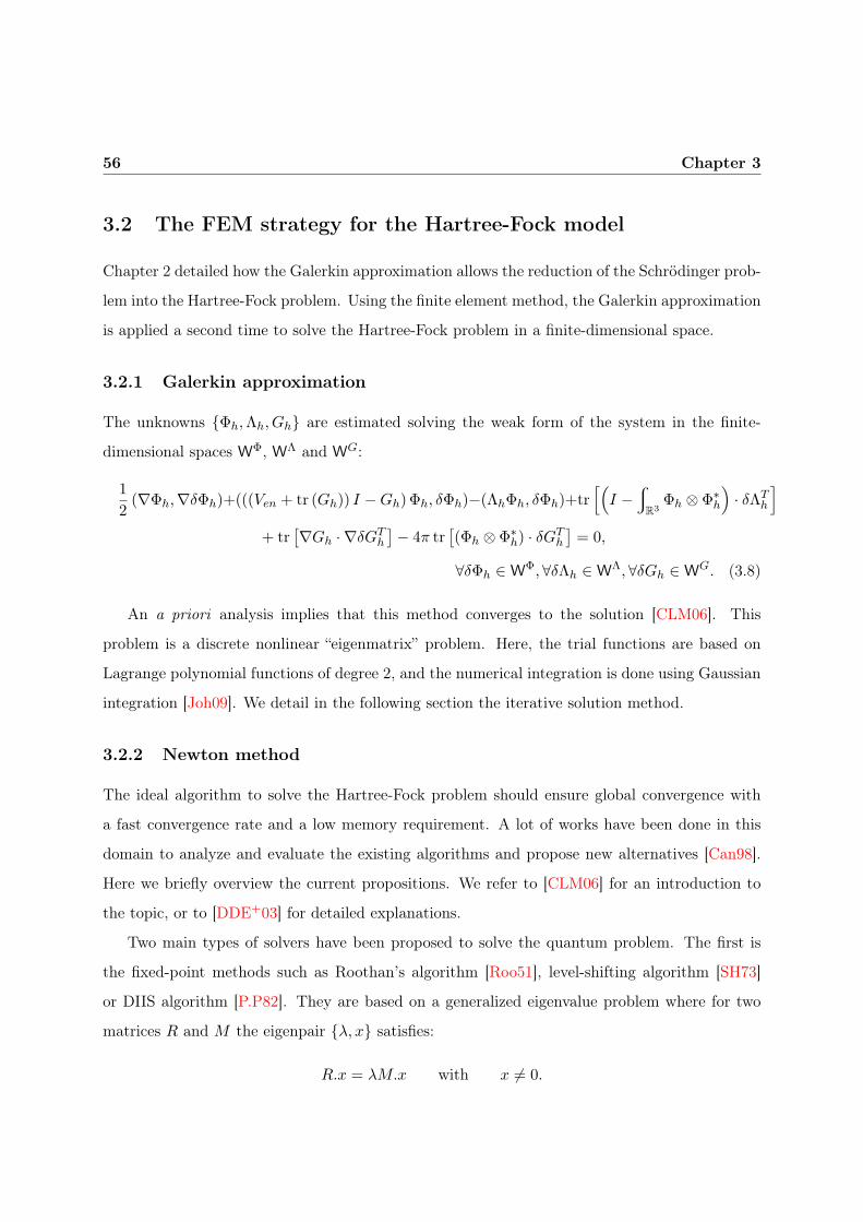
56 Chapter 3
3.2 The FEM strategy for the Hartree-Fock model
Chapter 2 detailed how the Galerkin approximation allows the reduction of the Schrödinger prob-
lem into the Hartree-Fock problem. Using the finite element method, the Galerkin approximation
is applied a second time to solve the Hartree-Fock problem in a finite-dimensional space.
3.2.1 Galerkin approximation
The unknowns Φh,Λh, Gh are estimated solving the weak form of the system in the finite-
dimensional spaces WΦ, WΛ and W
G:
1
2(∇Φh,∇δΦh)+(((Ven + tr (Gh)) I −Gh) Φh, δΦh)−(ΛhΦh, δΦh)+tr
[(
I −w
R3Φh ⊗ Φ∗
h
)
· δΛTh
]
+ tr[∇Gh · ∇δGT
h
]− 4π tr
[(Φh ⊗ Φ∗
h) · δGTh
]= 0,
∀δΦh ∈ WΦ, ∀δΛh ∈ W
Λ, ∀δGh ∈ WG. (3.8)
An a priori analysis implies that this method converges to the solution [CLM06]. This
problem is a discrete nonlinear “eigenmatrix” problem. Here, the trial functions are based on
Lagrange polynomial functions of degree 2, and the numerical integration is done using Gaussian
integration [Joh09]. We detail in the following section the iterative solution method.
3.2.2 Newton method
The ideal algorithm to solve the Hartree-Fock problem should ensure global convergence with
a fast convergence rate and a low memory requirement. A lot of works have been done in this
domain to analyze and evaluate the existing algorithms and propose new alternatives [Can98].
Here we briefly overview the current propositions. We refer to [CLM06] for an introduction to
the topic, or to [DDE+03] for detailed explanations.
Two main types of solvers have been proposed to solve the quantum problem. The first is
the fixed-point methods such as Roothan’s algorithm [Roo51], level-shifting algorithm [SH73]
or DIIS algorithm [P.P82]. They are based on a generalized eigenvalue problem where for two
matrices R and M the eigenpair λ, x satisfies:
R.x = λM.x with x 6= 0.

Numerical strategy 57
Roothan’s algorithm was historically the first algorithm used to tackle quantum problems. It
either converges towards a stationary point or oscillates between two states, none of them being
solution to the HF system. Currently, the most commonly used algorithm is the Direct Inversion
in the Iterative Subspace (DIIS) algorithm. It turns out to be very efficient in most cases, but
does not converge for some cases without rigorous explanation for that [CDK+03].
The second category of algorithms has been developed to solve the constraint optimization
problem. Different optimization algorithms are proposed in [CLM06]. They all consist in building
a sequence of iterates x which converges to the global minimizer of E. The next iterate xn+1
from xn is based on two choices: the choice of the direction dn, and the choice of the length tn
along this direction. These algorithms always converge but rarely towards the global minimum
for large systems or large function bases.
Full Newton method
Here we propose to apply Newton’s method to solve the system (3.8). The Newton method has
already been used by [FMS73] as an alternative to classical algorithms for solving the eigenvalue
problem . We detail the algorithm hereafter. For the sake of clarity, we describe it in the case of
the strong form of the system.
Starting from initial valuesΦ0,Λ0, G0
, the iterative process consists in building a series of
increments 0, 1, 2, . . . , n while convergence is not reached. We present here how the increments
are defined at the step n+ 1 from the values of the unknowns at step n. Let us first define the
residuals at iteration n:
rnΦ = −1
2∆xΦ
n + VenΦn + (tr (Gn) I −Gn) Φn − ΛnΦn,
RnG = −∆Gn − 4πΦn∗ ⊗ Φn,
RnΛ =
rR3 Φ
n∗ ⊗ Φn − I.
(3.9)
The Newton method stems from a linearization of the system around the last iterate Φn,Λn, Gn.

58 Chapter 3
At step n+ 1, the small increments dΛ, dΦ, dG must satisfy:
0 = rn+1Φ = rnΦ + dΛ (Φn) + Λn (dΦ) +
1
2∆xdΦ− VendΦ− (tr (dG) I − dG) Φn
− (tr (Gn) I −Gn) dΦ,
0 = Rn+1G = Rn
G +∆GdG+ 4π(dΦ⊗ Φn∗
+Φn ⊗ dΦ∗),
0 = Rn+1Λ = Rn
Λ −rR3
(dΦ⊗ Φn∗
+Φn ⊗ dΦ∗)dx.
(3.10)
The problem consists in finding dΛ, dΦ, dG while|dΛ|+ |dΦ|+ |dG||Λ|+ |Φ|+ |G| ≥ tol
max where |Λ| =√
tr (Λ.ΛT ) and |G| =√
tr (G.GT ).
The increments dΛ, dΦ, dG are defined from the solution of the linear system at step n. For
more clarity, we suppress indexes n:
Find dΛ, dΦ, dG such that:
−dΛ (Φ) + (tr (dG) I − dG) Φ +
(
−1
2∆x •+VenI + tr (G) I −G− Λ
)
︸ ︷︷ ︸
F
.dΦ = rΦ,
∆GdG+ 4π (dΦ⊗ Φ∗ +Φ⊗ dΦ∗) = RG,
rR3 (dΦ⊗ Φ∗ +Φ⊗ dΦ∗) dx = RΛ.
(3.11)
where F is the operator underlined in eq.(3.11). It is possible to eliminate successively dG:
dG = −∆−1G RG −∆−1
G (4π (dΦ⊗ Φ∗ +Φ⊗ dΦ∗)) = GR +GΦ (dΦ) . (3.12)
The increment dG has two origins: GR the inverse Green function of the residual RG, and
GΦ (dΦ) an increment proportional to the increment dΦ. Then, the increment dΦ can also be
eliminated:
dΦ = F−1 (rΦ + dΛ (Φ)− (tr (dG) I − dG) Φ) = Φr +ΦG +ΦΛdΛ. (3.13)
It has three origins: Φr the image of the residual rΦ by the inverse of the Fock operator, ΦG an
increment linked with the increment dG and ΦΛ (dΛ) an increment proportional to the increment
dΛ. Finally, dΛ reads:
w
R3(ΦΛdΛ)⊗s Φ dx = RΛ −
w
R3(Φr +ΦG)⊗s Φ dx. (3.14)

Numerical strategy 59
These loops are iterated until the convergence target error tolmax is reached. We generally
consider tolmaxgr = 10−6. One of the difficulties to solve the Hartree-Fock system is the very large
number of degrees of freedom. Figure 3.3 represents the number of functions to be evaluated
for atomic systems. For an unrestricted Hartree-Fock (UHF) strategy (see page 41), it increases
proportionally to the number of electronsNe asN1.6e . This drastic increase is due to the numerous
interaction terms Gij . For cases where a restricted Hartree-Fock (RHF) strategy can be set up,
the increase is reduced and proportional to N1.3e . For instance, the study of Chlorine, an atom
of 17 electrons, requires a UHF strategy and the estimation of 97 functions. Computing the
fundamental state of Argon, an atom of 18 electrons, requires only the estimation of 46 functions
by the RHF strategy.
Number of electrons
Num
ber
offu
ncti
ons
(ϕi,G
ij) Unrestricted HF
Restricted HF••
• • • •• •
• • •
•
•
•
••
••
•
•
0
20
40
60
80
100
0 5 10 15 20
Figure 3.3: Number of degrees of freedom in three-dimensional computations depending on the
number of electrons for atomic systems in RHF or UHF conditions
Staggered Newton method
Due to the number of unknowns, stiffness matrices associated with the vector Φ and the matrix G
are very large and their consideration in linear solvers can demand a lot of memory. A staggered
strategy is set up to reduce memory requirements. For each step towards convergence,

60 Chapter 3
initial mesh, Φ0, Λ0, G0 = f(Φ0), i = 1, n = 1, m = 1
Calculate the group i: ϕn,mi , Λn,m
ij , Gn,mij ∀ j ≤ i
ermgr < tol
maxgr ?
i < Ngr ?
ern < tol
max ?
dof > dofmin ?
Φf = Φn,m, Λf = Λn,m
yes
no
yes
yes
ϕn,m+1
i = ϕn,mi
Λn,m+1
ij = Λn,mij
Gn,m+1
ij = Gn,mij
∀ j ≤ i
m = m+ 1
i = i+ 1
Φn+1,0 = Φn,m
Λn+1,0 = Λn,m
Gn+1,0 = Gn,m
i = 1
n = n+ 1
m = 0
Refine mesh
no
yes
no
no
Figure 3.4: Scheme of the numerical strategy applied to the Hartree-Fock problem

Numerical strategy 61
the variables related to the same wave function i ϕi,Λji, Gji if j 6 i are lumped together in
Ngr groups.
Hn+111 Φn+1
1 +Hn12Φ
n2 = Λn+1
1 Φn+11
Hn12Φ
n1 +Hn+1
22 Φn+12 = Λn+1
2 Φn+12
Each group is estimated independently from the other ones. Therefore, the submatrices to be
inverted are much smaller. For the same memory cost, the number of nodes of the mesh can be
increased, and the accuracy of the results is improved. To optimize the accuracy of the results,
we can impose a constant number of functions by group and increase the number of groups, but
this alternative leads to an increase of the computation time.
It is important to note that all the components of the stiffness matrix relative to the matrix
G are identical. Memory requirement is reduced by saving the stiffness matrix and solving
simultaneously for different right-hand sides of the equation.
Figure 3.4 sums up the solution strategy. We use a staggered strategy and begin any com-
putation by determining the number of segregation groups Ngr. Then, three loops follow one
another. The first one estimates the unknowns relative to each group, when the other ones have
a fixed expression; the superscript m numbers the iteration, and the loop is stopped when the
error is inferior to the target error tolmaxgr . Once all the groups have been computed separately,
the error is estimated over all the unknowns. The second loop is iterated until the convergence
target error tolmax is reached. The iterations are numbered by n. The last loop controls the
number of degrees of freedom used to estimate any field ϕi or Gji and forces it to be superior to
dofmin.
Fixing the convergence criteria is a delicate task. Even if some authors propose results with
a high precision such as [OT11] which present results to the nearest 10−15 Ha, in most of the
litterature, energy estimates are provided experimentally or numerically to the nearest 10−3 Ha
[TCA08a, MHH12]. Usually, we choose tolmaxgr = 10−6, tolmax = 10−7 and dof
min = 100000, and
provide results to the nearest 10−4 Ha.
We now turn to the initial guesses applied to the iterative numerical method.
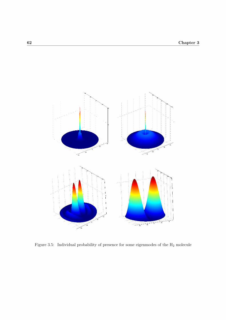
62 Chapter 3
Figure 3.5: Individual probability of presence for some eigenmodes of the H2 molecule

Numerical strategy 63
Starting values of the unknowns
It has been proven that the Hartree-Fock system has a discrete spectrum of several eigenvalues
and eigenfunctions [Lio87]. The Newton method used here provides only one solution. The
algorithm does not guarantee that this solution is the ground state solution. Fonte et al. proved
in [FMS73] the existence and the local uniqueness of a solution of the Hartree-Fock equations by
the Newton iteration algorithm in some specific mathematical conditions which depend on the
modes provided as initial guesses. We can check a posteriori that approximate wave functions
are the ground-state solution by examining the number of nodes of the solutions i.e. the number
of points where the wave function has minimal amplitude. If the approximate solution is not
the ground state, it can be any eigenmode of the eigenmode spectrum. Figure 3.5 illustrates
different eigenmodes of the H2 molecule.
In the case of atoms or molecules with ionic bonds, we impose as initial guesses the ground
state hydrogen-like atomic orbitals. We list them below using the spherical coordinate system and
denoting Zeff the effective nuclear charge that is the positive charge experienced by an electron
taking into account the shielding effect due to the other electrons:
Mode 1s: χ1s (r) =1√π
Z32eff
exp (−Zeff r),
Mode 2s: χ2s (r) =1
2√2π
Z32eff
(
1− Zeff r
2
)
exp
(
−Zeff r
2
)
,
Mode 2px: χ2px (r, θ, ϕ) =1
4√2πrZ
52eff
exp
(
−Zeff r
2
)
sin θ cosϕ,
Mode 2py : χ2py (r, θ, ϕ) =1
4√2πrZ
52eff
exp
(
−Zeff r
2
)
sin θ sinϕ,
Mode 2pz: χ2pz (r, θ) =1
4√2πrZ
52eff
exp
(
−Zeff r
2
)
cos θ,
Mode 3s: χ3s (r) =1
3√3π
Z32eff
(
1− 2Zeff r
3+
2Z2effr2
27
)
exp
(
−Zeff r
3
)
,
Mode 3px: χ3px (r, θ, ϕ) =4
27√2π
Z32eff
(
Zeff r −Z2
effr2
6
)
exp
(
−Zeff r
3
)
sin θ cosϕ,
Mode 3py: χ3py (r, θ, ϕ) =4
27√2π
Z32eff
(
Zeff r −Z2
effr2
6
)
exp
(
−Zeff r
3
)
sin θ sinϕ,
Mode 3pz: χ3pz (r, θ) =4
27√2π
Z32eff
(
Zeff r −Z2
effr2
6
)
exp
(
−Zeff r
3
)
cos θ.

64 Chapter 3
For molecules with covalent bonds, we can apply a linear combination of hydrogen-like or-
bitals, but predicting this linear combination is cumbersome for complex systems. Therefore,
initial values of the unknowns for molecules with covalent bonds are obtained as solutions of the
linearized system. The non-linear part is introduced gradually increasing the coefficient α from
0 to 1 like in a continuation method and we get for each α, Φ(α),Λ(α), G(α) defined by:
(
+1
2∇Φ,∇δΦ
)
+ ((Ven + α (tr (G) I −G)) Φ, δΦ) = (ΛΦ, δΦ) , ∀δΦ ∈ WΦ,
tr[∇G.∇δGT
]= tr
[(4πΦ⊗ Φ∗) .δGT
], ∀δG ∈ W
G,
tr[(I −
rR3 Φ⊗ Φ∗
).δΛT
]= 0, ∀δΛ ∈ W
Λ.
(3.15)
The first computation is made with α = 0. Then, the solution obtained is used as the initial
values of the functions for a computation considering α = δα. Iteratively, solutions obtained
when α = (n − 1) δα are used as initial values for computations with α = n δα until α = 1.
Generally, we impose δα = 0.2.
3.2.3 Artificial boundary conditions
The Hartree-Fock system is a set of equations defined on a three-dimensional unbounded space
whereas the FEM is conventionally designed to work on bounded domains. Even if infinite
elements [Ast00, Kum00], or generalized finite element method [NB76] can be possible strategies
to solve such problems, we choose to apply the FEM on bounded domains with special boundary
conditions.
For isolated systems, the FEM domain Ω is a sphere whose radius is R. To reduce parasite
effects of the external boundaries, the spherical boundary of the domain is chosen to be far from
the different nuclei. To limit the volume of computation to a sphere not too large, we introduce
artificial boundary conditions [EM77].
Far from the nuclei, we approximate wave functions as spherical waves:
ϕi|r→∞ = ϕ0 expikir . (3.16)

Numerical strategy 65
Neglecting the effect of Coulombian potentials in this area, we establish from the Hartree-Fock
system (2.24) that k2i = 2Λii. Therefore, in cases of materials at ground state (with negative
electronic energies), the boundary conditions for the wave functions Φ are:
∂ϕi
∂r
∣∣∣∣r→∞
= −√
−2Λiiϕi. (3.17)
The interaction terms Gij are approximate solutions of Laplace’s equations whose second terms
involve themselves the wave functions ϕi and ϕj . The radial approximation at the boundary is
difficult to establish. We write it from the convolution form defined by eq.(2.16):
∂Gij
∂r
∣∣∣∣r→∞
=(
−√
−2Λii −√
−2Λjj
)
Gij . (3.18)
External boundary conditions imply some parasite effects, especially when the size of the FEM
domain gets smaller. In Table 3.2, we compare the energy estimates for the Helium atom applying
aforesaid conditions and Dirichlet conditions that impose approximate wave functions to vanish
on the spherical boundary. In the case of the Helium atom, we conclude that a radius greater
than 20 a0 is large enough to cancel the effect of the type of boundary conditions. However, the
boundary can have an effect due to the estimation of the energy defined by the integral on a
bounded domain of Equation (2.23), whereas the quantum problem is defined on an unbounded
domain.
Radius of the domain (a0) Order of magnitude of the difference
in estimates of electronic energy
between radiative and Dirichlet conditions (Ha)
5 10−4
10 10−9
15 10−15
≥ 20 < 10−15
Table 3.2: Influence of the boundary conditions on the estimation of the energy of the Helium
atom for different radii of the FEM domain

66 Chapter 3
3.2.4 Mesh and adaptivity
We use tetrahedrons to partition the three-dimensional FEM domain. For axisymetrical modes as
explained below, triangular elements mesh the FEM domain. With real-space methods, localized
refinement seems appealing to optimize the number of degrees of freedom, and perform large
scale ab initio calculations. As wave functions present a singularity near the nuclei, we impose
an initial mesh refined in these critical zones. Another approach would be to use generalized
finite element method [NB76].
Adaptive coordinate transformations [TT96, TT98] or self-adaptive meshing [AR93] allow
to locally refine the estimation of the wave functions. To improve the quality of the numerical
solution, we employ a mesh adaptivity method and ensure that a minimum number of degrees
of freedom dofobj is used to estimate any function. The mesh is optimized with respect to the
local error.
Adaptivity can be set up for different quantities of interest and different norms. We use the
L2 norm. The mesh and so the results depend on the quantity considered to refine the mesh.
(a) Initial mesh (b) Adaptivity on (c) Adaptivity on (d) Adaptivity on
all the unknowns the 2s mode the 2pz mode
19 453 dof 109 081 dof 150 017 dof 131 621 dof
Figure 3.6: Meshes of adaptive computations for the Neon atom on a FEM domain of radius 40 a0:
Initial mesh (a) and different meshes obtained after two adaptive iterations (b,c,d)
Figure 3.6 presents different meshes obtained after two iterative steps for different quantities

Numerical strategy 67
of interest. Considering all unknowns, new nodes are evenly added into the FEM domain.
Considering a localized wave function such as the 2s mode, the new nodes are localized in a
small area near the nucleus. For a less localized wave function such as the 2pz mode, nodes are
added in a larger area around the nucleus. Considering the error on the interaction terms Gij ,
the mesh is refined far from the nucleus.
As the error estimator is not unique, the choice of an accurate estimator is crucial. Chapter 5
focuses on this topic. For the first calculations presented here, error is estimated with respect to
all unknowns using the Euclidian norm based on the local residual.
3.2.5 Symmetry simplifications for atoms and linear molecules
In the case of atoms and linear molecules i.e. molecules in which all bond angles are 180 degrees,
all one-electron wave functions can be broken up into two independent functions: in-plane func-
tions ϕrzi depending on the two dimensions r and z, and axial functions ϕθ
i depending only on
the angle θ [Bre30]:
ϕi(r, θ, z) = ϕθi (θ)ϕ
rzi (r, z). (3.19)
In these cases, axial functions ϕθi are spherical harmonics that depend on the magnetic quantum
number mi (defined in Appendix E) of the wave function considered:
ϕθi (θ) = eimiθ. (3.20)
For more general cases, a spherical harmonics development would be possible. The “building-
up” principle, also called the Aufbau principle, allows for the knowledge a priori of the second
quantum number mi of each one-electron wave function, and so the electron configuration of the
different atoms (Appendix D).
The FEM domain can be reduced to a two-dimensional one, a half-disk whose radius is denoted
R: Ω = (r, z), r ≥ 0,√r2 + z2 6 R. In some peculiar cases, due to the symmetry of the wave
functions, we could use only a quarter of a disk.
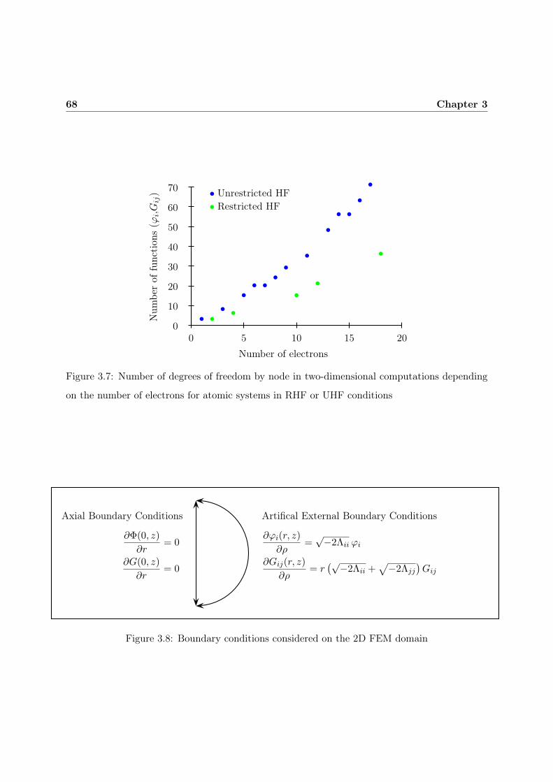
68 Chapter 3
Number of electrons
Num
ber
offu
ncti
ons
(ϕi,G
ij) Unrestricted HF
Restricted HF••
• •• •
•• •
••
•
•
•
•• •
••
•
0
10
20
30
40
50
60
70
0 5 10 15 20
Figure 3.7: Number of degrees of freedom by node in two-dimensional computations depending
on the number of electrons for atomic systems in RHF or UHF conditions
Axial Boundary Conditions
∂Φ(0, z)
∂r= 0
∂G(0, z)
∂r= 0
Artifical External Boundary Conditions
∂ϕi(r, z)
∂ρ=
√−2Λii ϕi
∂Gij(r, z)
∂ρ= r
(√−2Λii +
√−2Λjj
)Gij
Figure 3.8: Boundary conditions considered on the 2D FEM domain

Numerical strategy 69
In the two-dimensional space (r, z), find (ϕrzi ,Λij) such that:
(Ne∑
j=1ei(mj−mi)θΛijϕ
rzj , δϕ
rzi
)
= −1
2
[
(∇rzϕrzi ,∇rzδϕ
rzi )−
(m2
i
r2ϕrzi , δϕ
rzi
)]
+
((
Ven + trGrz −Ne∑
j=1Grz
ji
)
ϕrzi , δϕ
rzi
)
,
tr(
∇rzGrzij .∇rzδG
rzij
)
− (mi −mj)2
r2
(
Grzij , δG
rzij
)
= tr((
4πϕrzi ⊗ ϕrz∗
j
)
.δGrzTij
)
,
tr((
Iij − ei(mi−mj)rR3 ϕ
rzi ⊗ ϕrz∗
j
)
.δΛTij
)
= 0,
∀δϕi ∈ Wϕ, ∀δGij ∈ W
Gij , ∀δΛij ∈ WΛij .
(3.21)
The derivation of the weak formulation in two-dimensional space is detailed in Appendix H.
We have calculated systems for which the second quantum number is equal to -1, 0 or 1. These
three values of the second quantum number match three degenerate eigenmodes. The equations
are identical for the values +m or −m of the second quantum number. We choose to calculate
only the eigenmodes for the non-negative values of mi. This strategy leads to a decrease of the
number of functions to be computed and to get rid of degeneracy between the three modes.
Figure 3.7 shows how the number of unknowns is reduced considering only the positive values
of mi.
For instance, to compute the fundamental state of argon, the number of functions to be
evaluated is reduced from 46 to 35. Figure 3.9 shows how the three-dimensional solutions are
built once the two-dimensional modes have been computed.
For the axial boundary (r = 0), supposing ϕi = eimiθϕrzi (r, z), the boundary conditions
depend on the parity of mi for the one-electron wave function ϕi:
∃k ∈ N mi = 2k∂ϕi(0, z)
∂r= 0,
∃k ∈ N mi = 2k + 1 ϕi(0, z) = 0.
(3.22)
and for the components Gij of the matrix G:
∃k, k′ ∈ N2, mi = 2k and mj = 2k′,
∂Gij(0, z)
∂r= 0,
else, Gij(0, z) = 0.
(3.23)

70 Chapter 3
2D 1st and 2nd modes =⇒ 3D 1st and 2nd modes (|ϕ1|2 = 0.13)
2D 3rd and 4th modes =⇒ 3D 3rd and 4th modes (|ϕ3|2 = 0.13)
2D 5th and 6th modes =⇒ 3D 5th and 6th modes (|ϕ5|2 = 0.13)
2D 7th and 8th modes =⇒ 3D 7th and 8th modes (|ϕ7|2 = 0.13)
Figure 3.9: Probability of presence of the different modes of the Oxygen atom in two-
dimensional (r, z) and three-dimensional (r, θ, z) spaces

Numerical strategy 71
For the circular external boundary (ρ = R), as developed for three-dimensional cases, we use a
plane wave approximation far from the nuclei and we subject the one-electron wave functions ϕi
to the following boundary condition:
∂ϕi(r, z)
∂ρ=√
−2Λii ϕi, (3.24)
and the components Gij of the matrix G, solution of Laplace’s equations, to:
∂Gij(r, z)
∂ρ= r
√
m2i
r2− 2Λii +
√
m2j
r2− 2Λjj
Gij . (3.25)
Figure 3.8 illustrates the boundary conditions for the vectors Φ and G in the particular case of
all the wave functions have a second quantum number which equals 0.
3.3 Summary
In this chapter, the finite element method strategy used to solve the Hartree-Fock system is
presented. This numerical method combines the advantages of both basis-oriented and real-
space-grid approaches. We choose as the iterative method the Newton method and evaluate
residuals at each step. The calculation is stopped when convergence on a quantity of interest
(such as the total energy, or the wave function itself. . . ) is obtained.
Difficulties in solving the Hartree-Fock system lie in the number of degrees of freedom, the
singularities of the wave functions and the different eigenfunctions which can be solution of
the system. To overcome difficulties due to the number of degrees of freedom, the algorithm
integrates a staggered solver and mesh adaptivity. Initial guesses are hydrogen orbitals or the
solutions of the linearized problem. But, the algorithm does not guarantee to provide a global
optimizer. The number of nodes of the solution wave functions is checked a posteriori for being
equal to the number of nodes of the expected modes.
This chapter has introduced the numerical strategy for the Hartree-Fock problem. The same
approach is used to compute the virtual modes and estimate the CI energy. The CI model is used
to increase the accuracy of the estimation and needs a large FEM domain, and a large number
of degrees of freedom to be pertinent. But, with a large radius of the FEM domain, it is difficult
to obtain convergence of the virtual modes.

72 Chapter 3
BeH
HBeH
HBeH
H
ϕ1 ϕ2 ϕ3
1st mode 2nd mode 3rd mode
e1 = −4.6685 Ha e2 = −0.5020 Ha e3 = −0.4510 Ha
BeH
HBeH
HBeH
H
G11 G22 G33
BeH
HBeH
HBeH
H
G12 G13 G23
Figure 3.10: Fields computed for the Hartree-Fock modelization of the ground state of the BeH2
molecule

Numerical strategy 73
Figure 3.10 shows the different two-dimensional fields computed to characterize the BeH2
molecule (composed of three atoms and six electrons): three one-electron wavefunctions ϕ1, ϕ2,
ϕ3 and six interaction terms G11, G22, G33, G12, G13 and G23.
3.4 Large scale perspectives
The Hartree-Fock or post-Hartree-Fock problems are generalized eigenvalues problems. These
problems have cubic complexity, which is the bottleneck in dealing with many electron systems.
Different strategies have been developed to overcome this difficulty [CA08].
To circumvent the curse of dimensionality, a reduced basis approximation method is suggested
by Maday and Razafison [MR08]. They consider a space of approximation smaller than the
usual Hartree-Fock space, it is spanned by a small number of well chosen solutions. Other
authors propose a separated representation strategy [AMCK06a, AMCK06b, AC08] or Proper
Generalized Decomposition [Nou10]. This strategy can be seen as elaborate derivative of the
decomposition on atomic orbitals basis.
By a modal analysis, a first strategy consists in computing only the significant modes. Only
the modes that can participate in the formation of chemical bonds are involved in material prop-
erties, they are called valence modes [vBG80]. Modes that are not perturbed by the surrounding
atoms such as the first mode of the Beryllium atom (Figure 3.11) are called core modes. An
idea to reduce the complexity of the calculation is to compute only the valence modes. Core
electrons are included into nuclear potentials through pseudopotentials or core effective poten-
tials [Pic89]. These potentials are established by preliminary computations on isolated atoms.
Technical aspects of this method are explained in [PTA+92].
Solutions of electronic problems are generally localized and pertinent information is only given
by the valence modes outside the regions surrounding nuclei [YC82]. To take advantage of this
property, Slater proposed in 1937 a localized model refinement called the muffin-tin approxima-
tion to treat periodic materials [Sla37]. Potentials between nuclei and electrons were supposed to
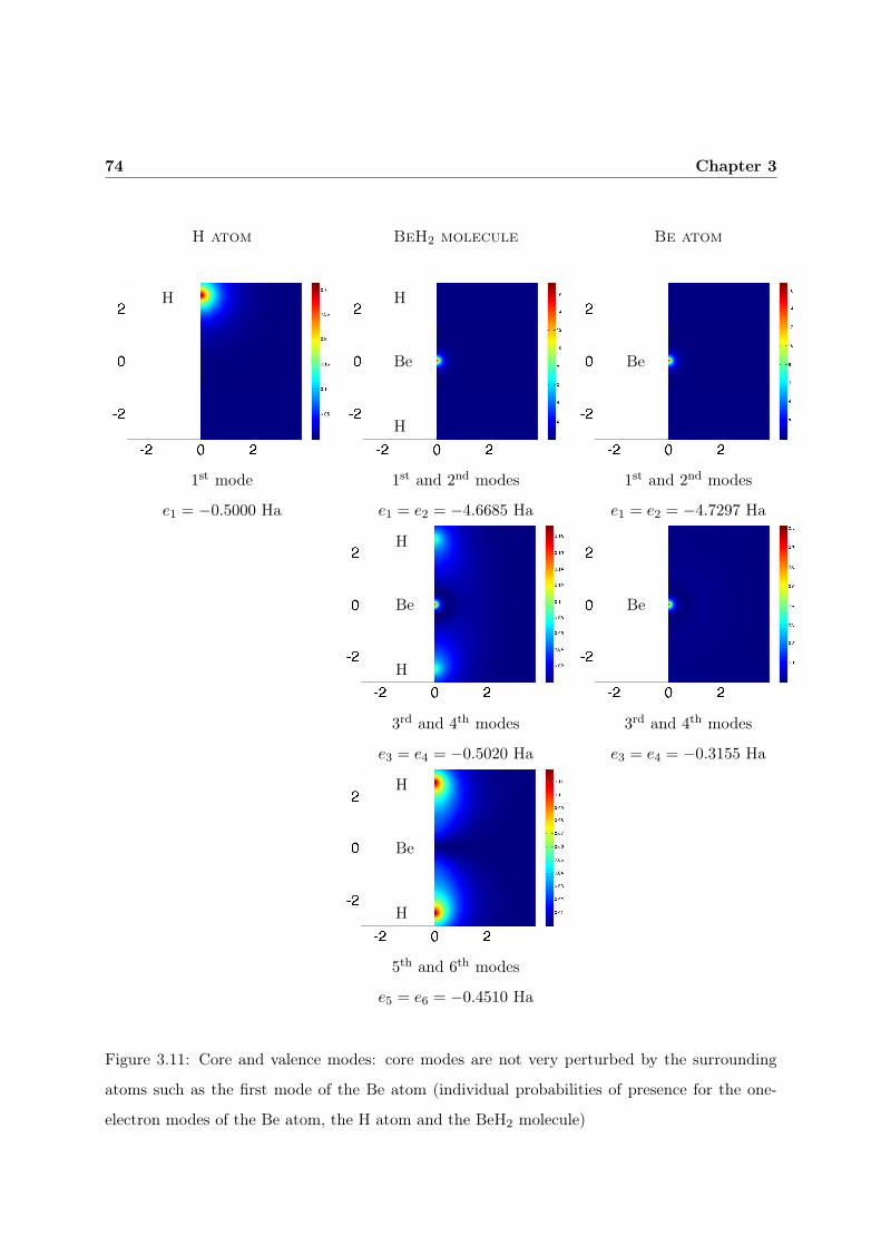
74 Chapter 3
H atom BeH2 molecule Be atom
H
Be
H
H
Be
1st mode 1st and 2nd modes 1st and 2nd modes
e1 = −0.5000 Ha e1 = e2 = −4.6685 Ha e1 = e2 = −4.7297 Ha
Be
H
H
Be
3rd and 4th modes 3rd and 4th modes
e3 = e4 = −0.5020 Ha e3 = e4 = −0.3155 Ha
Be
H
H
5th and 6th modes
e5 = e6 = −0.4510 Ha
Figure 3.11: Core and valence modes: core modes are not very perturbed by the surrounding
atoms such as the first mode of the Be atom (individual probabilities of presence for the one-
electron modes of the Be atom, the H atom and the BeH2 molecule)

Numerical strategy 75
be spherically symmetrical within spheres surrounding the atoms, and constant outside. Wave
functions were expanded in spherical harmonics and radial solutions of the wave equations within
the spheres, and in plane waves outside the spheres, joining continuously at the surface.
Recently, Barrault [Bar05, BCHLB07] applied a technique of domain decomposition and
turned the unique problem into several localized minimization problems under constraint. He
showed a localized convergence of the algorithm, scalability up to 1000 processors in 1D and
possible extension to 2D/3D domains. The domain decomposition method provides linear com-
plexity with respect to the number of electrons in the system.


Chapter 4
Ab initio quantities of interest
This chapter is devoted to the numerical results obtained by the Hartree-Fock method described
in Chapter 2 and the numerical strategy detailed in Chapter 3. First, we focus on the individual
electronic wave functions that completely describe any atomic system. Then, we exploit them to
provide other physical information: mechanical quantities such as bonding forces, bond stiffness,
or electric properties such as dipolar moment and polarizability tensor.
4.1 The one-electron wave functions
Quantum mechanical computations provide the wave function of the system. In the case of the
Hartree-Fock model, we compute the one-electron wave functions. In two-dimensional computa-
tions, each one-electron wave function is described by its field in the plane (r, z) and its magnetic
quantum number.
We only examine the one-electron wave functions of the ground state.
4.1.1 Geometrical distribution of the individual wave functions
Figure 4.1 and Figure 4.2 represent, respectively, the probability of presence of the one-electron
wave functions of the Beryllium and the Oxygen atoms. In both cases, the nucleus of the atom
is located in (0; 0). We note that all individual wave functions are localized in an area near the
nucleus. The probability of presence decreases rapidly to almost vanish far from the nucleus. To

78 Chapter 4
1st and 2nd modes (m1=m2=0) 3rd and 4th modes (m3=m4=0)
e1 = e2 = −4.7297 Ha e3 = e4 = −0.3155 Ha
R99,1 = R99,2 = 1.11 a0 R99,3 = R99,4 = 5.53 a0
Figure 4.1: Individual probability of presence for the ground-state modes of the Beryllium atom
(HF model)

Ab initio quantities of interest 79
1st and 2nd modes (m1=m2=0) 3rd and 4th modes (m3=m4=0)
e1 = −20.7343 Ha e3 = −1.4293 Ha
e2 = −20.6594 Ha e4 = −1.0939 Ha
R99,1 = R99,2 = 0.4959 a0 R99,3 = 2.3880 a0
R99,4 = 2.4796 a0
5th and 6th modes (m5=m6=0) 7th (m7=1) and 8th (m8=−1) modes
e5 = −0.6265 Ha e7 = e8 = −0.6335 Ha
e6 = −0.5389 Ha
Figure 4.2: Individual probability of presence for the different modes of the Oxygen atom
(HF model)

80 Chapter 4
e1 = −4.7297 Ha e2 = −0.3155 Ha
m1 = 0 m2 = 0
Be atom
e1 = −20.7343 Ha e3 = −1.4293 Ha e5 = −0.6265 Ha e7 = e8 = −0.6335 Ha
e2 = −20.6594 Ha e4 = −1.0939 Ha e6 = −0.5389 Ha
m1 = 0 m2 = 0 m3 = 0 m4 = 1
O atom
Figure 4.3: Profiles of the one-electron wave functions in the r direction (in blue) and in the z
direction (in red) for the Beryllium atom and the Oxygen atom (HF model)

Ab initio quantities of interest 81
characterize the extent of the modes, we define a distance R99 as the radius of a sphere in which
the probability of presence of all the electrons is 99%.
The Beryllium atom comprises four electrons whereas the Oxygen atom contains eight elec-
trons. We can see that when the number of electrons in the atom increases, the new occupied
modes are more diffused far from the nucleus.
Comparing the different modes of a same atom in Figure 4.3, we observe that the more
diffused modes are those with the highest eigenvalues. The number of nodes, zeros of the wave
functions, increases with the frequency of the stationary system and so with the energy of the
modes.
Among all the stable natural elements, we focus our study on the isolated atoms of the elements
between the hydrogen and calcium atoms in the periodic table because these elements are pre-
ponderant in the chemical makeup of traditional materials. Results are introduced in Table 4.1.
For instance, let us examine the estimation for the Helium atom. The energy of the Helium
atom is estimated to be −2.86412 Ha which is far from the experimental estimation −2.901
Ha [DHC91] considered as “exact” estimation. The configuration interaction approximation im-
proves the estimation to −2.86413 Ha using 10 determinants. Comparing with other numerical
solutions of the Hartree-Fock problem (−2.8552 Ha [JGP93] and −2.8612 Ha [Kob12]), we can
see that our result is in concordance with the literature data. A better accuracy would need a
refined model considering dynamic and relativistic effects. For other atoms, the comparison is
similar. For instance, [JGP93] provides for the Lithium atom the HF total energy 7.4314 Ha
whereas our estimation is 7.4351 Ha (experimental estimation: 7.47821 Ha [DHC91]).
Beyond isolated atoms, we investigate the one-electron wave functions of systems in which
different nuclei are linked to form an isolated molecule.
4.1.2 Individual wave functions in bonds
In the case of molecules, the one-electron wave functions allow for an understanding of the
bonding state of the molecule and how the different electrons are involved in the bond. In

82 Chapter 4
Atom Z 1st mode 2nd mode 3rd mode 4th mode 5th mode 6th mode
H 1 -0.5000
He 2 -0.9185
Li 3 -2.4786 -0.1983
Be 4 -4.7297 -0.3155
B 5 -7.69275 -0.5033 -0.3208
C 6 -11.3263 -0.7077 -0.4389
N 7 -15.6539 -0.9595 -0.5477
O 8 -20.6969 -1.2616 -0.5996
F 9 -26.32485 -1.5571 -0.746125
Ne 10 -32.8242 -1.9622 -0.8082
Na 11 -40.3591 -2.7646 -1.6000 -0.1868
Mg 12 -49.4694 -4.1683 -2.6193 -0.1263
Al 13 -58.3814 -4.8939 -3.3419 -0.4027 -0.2379
Ar 18 -118.6267 -12.3322 -9.4544 -1.2929 -0.5867
Ca 20 -152.941 -17.0782 -13.4365 -2.2930 -1.3202 -0.2127
Table 4.1: Estimation of the electronic energy for ground-state one-electron modes for isolated
atoms (in hartree) considering R = 2000 a0 and 200 000 dof by function

Ab initio quantities of interest 83
Figures 4.4, 4.5, 4.6 and 4.7, we represent respectively the one-electron wave functions of the
LiH, HF, C2 and BeH2 molecules, and of the isolated atoms that compose them.
Some one-electron wave functions in the molecules have a very similar shape and energy to
those of the isolated atoms. The electrons associated with those wave functions are core electrons
of the atoms which are very stable and little disturbed by their surroundings. On the other hand,
some modes in the molecule have been largely disturbed when compared with those of isolated
atoms. The electrons associated with those modes are the valence electrons; they create the
bond between the atoms to form the molecule. The way the valence electrons behave to form the
bond characterizes the material. For prevailing covalent character of the bond, the one-electron
wave functions are “shared” between atoms (for instance in C2, BeH2 or O2 molecules). If some
one-electron wave functions initially centered around one nucleus are delocalized around another
nucleus, the bond is considered as ionic such as in the HCl, NaH or HF molecules.
Studying the one-electron wave functions is cumbersome due to the number of fields to be
examined, and assessment of the results is strenuous. To overcome these problems, we can focus
on the global electronic density of the system.
4.2 The electronic density
The electron density defined by equation (1.40) provides a unique field to analyze and understand
the bonding state of the system. Its approximation by the Hartree-Fock model reads:
ρHF (x) = |Φ|2. (4.1)
Using the CI model (see Chapter 2), it is evaluated by:
ρCI (x) =
Nd∑
k=1
|αk|2|Φk|2 +Nd∑
K=1
Nd∑
L=1L 6=K
αKα∗LδϕK
1 ϕL1. . . ϕK
a ϕL∗
a . . . δϕKNe
ϕLNe. (4.2)
where δϕKi ϕL
i= 1 if ϕK
i = ϕLi and δϕK
j ϕLi= 0 if ϕK
i 6= ϕLi . Figure 4.9 illustrates these electronic
densities, and so the bonding character, in the H2, LiH, BeH2, HF, NaH, HCl, and C2 molecules.
It can be compared with experimental results obtained by analyzing diffraction results. New
techniques are developped to measure directly the wave functions [LSP+11]. We present here
only results for isolated systems, for which we cannot provide diffraction results.
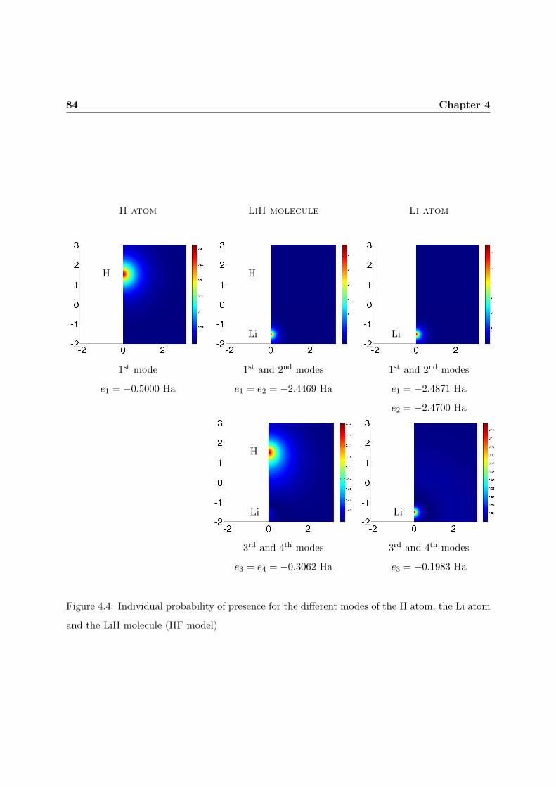
84 Chapter 4
H atom LiH molecule Li atom
H
Li
H
Li
1st mode 1st and 2nd modes 1st and 2nd modes
e1 = −0.5000 Ha e1 = e2 = −2.4469 Ha e1 = −2.4871 Ha
e2 = −2.4700 Ha
Li
H
Li
3rd and 4th modes 3rd and 4th modes
e3 = e4 = −0.3062 Ha e3 = −0.1983 Ha
Figure 4.4: Individual probability of presence for the different modes of the H atom, the Li atom
and the LiH molecule (HF model)

Ab initio quantities of interest 85
H atom HF molecule F atom
H
F
H
F
1st mode 1st and 2nd modes 1st and 2nd modese = −0.5000 Ha e = −26.3504 Ha e = −26.3249 Ha
F
H
F
3rd and 4th modes 3rd and 4th modese3 = e4 = −1.6264 Ha e3 = e4 = −1.5571 Ha
F
H
F
5th and 6th modes 5th and 6th modese5 = e6 = −0.7970 Ha e5 = e6 = −0.6831 Ha
F
H
F
7th, 8th, 9th and 10th modes 7th, 8th and 9th modese7 = e8 = e9 = e10 = −0.5858 Ha e7 = e8 = e9 = −0.8092 Ha
Figure 4.5: One-electron probability of presence of the H atom, the F atom and the HF molecule
(HF model)

86 Chapter 4
H atom BeH2 molecule Be atom
H
Be
H
H
Be
1st mode 1st and 2nd modes 1st and 2nd modes
e1 = −0.5000 Ha e1 = e2 = −4.6685 Ha e1 = e2 = −4.7297 Ha
Be
H
H
Be
3rd and 4th modes 3rd and 4th modes
e3 = e4 = −0.5020 Ha e3 = e4 = −0.3155 Ha
Be
H
H
5th and 6th modes
e5 = e6 = −0.4510 Ha
Figure 4.6: Covalent bond: individual probability of presence for the modes of the Be atom, the
H atom and the BeH2 molecule (HF model)

Ab initio quantities of interest 87
C atom C2 molecule C atom
C C
C C
1st and 2nd modes 1st and 2nd modes 1st and 2nd modes
e1 = −11.3487 Ha e1 = e2 = −11.3653 Ha e1 = −11.3487 Ha
e2 = −11.3038 Ha e2 = −11.3038 Ha
C C
C C
3rd and 4th modes 3rd and 4th modes 3rd and 4th modes
e3 = −0.8303 Ha e3 = e4 = −11.3287 Ha e3 = −0.8303 Ha
e4 = −0.5851 Ha e4 = −0.5851 Ha
C C
C C
5th mode 5th and 6th modes 5th mode
e5 = −0.4420 Ha e5 = e6 = −0.9321 Ha e5 = −0.4420 Ha

88 Chapter 4
CC
C C
6th mode 7th and 8th modes 6th mode
e6 = −0.4358 Ha e7 = e8 = −0.4321 Ha e6 = −0.4358 Ha
C
C
9th, 10th, 11th and 12th modes
e9 = e10 = e11 = e12 = −0.4283 Ha
Figure 4.7: Individual probability of presence for the different modes of the C atom and the C2
molecule (HF model)

Ab initio quantities of interest 89
We focus on the energy of the system to determine the nuclei positions at equilibrium.
4.3 Prediction of molecular geometry
We compute the total energy of the system by the Hartree-Fock model and by the configuration
interaction model. The positions of the nuclei at equilibrium match the minimum of the total
energy.
For instance, for an isolated molecule of H2, Figure 4.8 represents the total energy of the
H2 molecule as function of the bond length. We estimate the equilibrium bond length would
be 1.41 a0, which is in concordance with literature data [DG89]. We note that to determine
the equilibrium bond length to the nearest 0.01 a0, we need estimate of the total energy of the
system to the nearest 10−4 Ha. To predict this quantity to the nearest 0.001 a0, we should need
estimation of the total energy of the system to the nearest 10−6 Ha.
1 1.2 1.4 1.6 1.8 2
−1.14
−1.12
−1.1
−1.08
−1.06
Bond length (a0)
Tot
al e
nerg
y (H
a)
Figure 4.8: Total energy of the H2 molecule as function of the bond length (R = 2000 a0 and
dof = 200000)

90 Chapter 4
H
H
Li
H
Be
H
H
H2 LiH BeH2
H
F
H
Na
H
Cl
HF NaH HCl
C
C
C2
Figure 4.9: Computed electronic density for different molecules by HF

Ab initio quantities of interest 91
4.4 Mechanical properties
The first mechanical quantity we derive from quantum computations is the stress tensor defined
by equation (1.2). To evaluate the derivative of the energy with respect to the deformation, we
can compute the fundamental energy for different positions of the nuclei near the equilibrium
position, as illustrated on Figure 4.8. The value of the energy is estimated in each case and a
plot of energy vs deformation is obtained. The slope of this curve is the derivative of the energy
with respect to the deformation. The shortcoming of this method is the need to compute many
times the same molecule for different bond lengths.
4.4.1 Stress computation
Computing the forces at a given configuration without calculating at neighboring configura-
tions can be done from the perturbation expression of the energy using the Hellmann-Feynman
theorem [Fey39]. The stress tensor σ is defined as:
δE
Ω= tr (σ.ε)
where E is the total energy of the system, Ω the volume associated with this energy and ε is
the homogenized deformation due to the nuclei displacements δXNjsuch that δXNj
= ε(XNj
).
From equation (1.33), a variation of the total Hamiltonian δH implies a variation of the wave
function δΨ and of the total energy δE which satisfies:
(H − E) δΨ+ (δH − δE)Ψ = 0. (4.3)
As Ψ is the normalized solution of the Schrödinger problem, considering the product of equa-
tion (4.3) with Ψ∗, we have:
δE = (δHΨ,Ψ) . (4.4)
Considering there is no external electric field, the variation of the total energy of the system is
expressed as a function of the variation of the total hamiltonian:
δH = δVen + δVnn =
Nn∑
C=1
∇XC
VCe +
Nn∑
K=1K 6=C
∇XCVCK , ε (XC)

92 Chapter 4
where XC is the coordinate of the nucleus C. The interaction potentials (defined page 14) reads
VCe =−ZC
|x−XC |and VCK =
ZCZK
|XC −XK | . The gradients read:
∇XCVCe = −ZC
x−XC
|x−XC |3and ∇XC
VCK = ZCZKXC −XK
|XC −XK |3 . (4.5)
Therefore,
δE =
Nn∑
C=1
w
R3Ne−ZC
x−XC
|x−XC |3|Ψe|2dx+
Nn∑
K=1K 6=C
ZCZKXC −XK
|XC −XK |3 , ε (XC)
. (4.6)
We see through this formula that the variation of the nucleus-electron interaction energy due
to the deformation is the mean of the Coulomb potential gradient with respect to the deformation
weighted by the probability of presence of the particles. To identify the stress tensor, we express
the variation of the energy as the trace of a tensor:
δE = tr
Nn∑
C=1
w
R3Ne−ZC
x−XC
|x−XC |3|Ψe|2dx+
Nn∑
K=1K 6=C
ZCZKXC −XK
|XC −XK |3
⊗ ε (XC)
. (4.7)
As a⊗A(b) = [a⊗ b] .AT , the stress tensor reads:
σ =1
Ω
Nn∑
C=1
w
R3Ne−ZC
x−XC
|x−XC |3|Ψe|2dx+
Nn∑
K=1K 6=C
ZCZKXC −XK
|XC −XK |3
⊗S XC . (4.8)
The stress tensor is built-up from three effects:
• the interaction between nuclei,
• the interaction between nuclei and electrons,
• the interaction between nuclei and the external electric field.
Considering the Hartree-Fock approximation, it can be expressed as:
σHF =1
Ω
Nn∑
C=1
(
−ZCx−XC
|x−XC |3|Ψe|2Φ,Φ
)
+
Nn∑
K=1K 6=C
ZCZKXC −XK
|XC −XK |3
⊗S XC . (4.9)

Ab initio quantities of interest 93
This can be computed easily from the HF available integrals. Additionnally, using the configu-
ration interaction approximation, we have:
σCI =1
Ω
Nn∑
C=1
Nd∑
A=1
Nd∑
B=1
αAα∗B
(
−ZCx−XC
|x−XC |3|Ψe|2ΦA,ΦB
)
+
Nn∑
K=1K 6=C
ZCZKXC −XK
|XC −XK |3
⊗SXC .
(4.10)
We get thus the following result: Provided nuclei positions and the solution of the Schrödinger
equation, the stress tensor σ can be estimated from nucleus-nucleus and nucleus-electron dipoles.
As a generalization from atomic electrostatics, the dipoles are added for each atomic particle but
are weighted by the probability of presence for electrons.
4.4.2 Elasticity tensor computation
The elasticity tensor describes the linear elastic behavior of the material:
σ = C (ε) .
It can be computed from the second-order variation of the energy of the system submitted to
an homogeneous deformation defined before, and appears as the coefficient of the quadratic
expansion of the strains:
δ2E = tr [C (ε) .ε] .
As Ψe is the normalized solution of the Schrödinger equation, it can be shown from Equation (4.3)
that:
δ2E = 2(
(δH − δE) δΨ⊥,Ψ)
+(δ2HΨ,Ψ
)(4.11)
where δΨ⊥ = − (H − E)−⊥ (δV − δE)Ψ and (H − E)−⊥ stands for the orthogonal inverse of
this operator.
δ2E = −2(
(∇XNVNK , ε (XN ))− ((∇XN
VNe, ε (XN ))Ψ,Ψ)2 (H − E)−⊥Ψ,Ψ)
+(D2
XNXM(VNK + VNe) (Ψ,Ψ) (ε (XN )) , ε (XM )
)
The elasticity tensor C is calculated by the following expression:
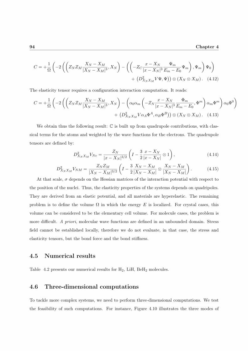
94 Chapter 4
C = +1
Ω
(
−2
((
ZNZMXN −XM
|XN −XM |3 , XN
)
−((
−ZCx−XN
|x−XN |3Ψm
Em − E0Ψm
)
,Ψm
)
Ψ0
)
+(D2
XNXMVΨ,Ψ
))⊗ (XN ⊗XM ) . (4.12)
The elasticity tensor requires a configuration interaction computation. It reads:
C = +1
Ω
(
−2
((
ZNZMXN −XM
|XN −XM |3 , XN
)
−(
α0αm
(
−ZNx−XN
|x−XN |3Φm
Em − E0,Φm
)
αmΦm
)
α0Φ0
)
+(D2
XNXMV αAΦ
A, αBΦB))
⊗ (XN ⊗XM ) . (4.13)
We obtain thus the following result: C is built up from quadrupole contributions, with clas-
sical terms for the atoms and weighted by the wave functions for the electrons. The quadrupole
tensors are defined by:
D2XNXM
VNe =ZN
|x−XN |3/2(
I − 3
2
x−XN
|x−XN | ⊗ 1
)
, (4.14)
D2XNXM
VNM =ZNZM
|XN −XM |3/2(
I − 3
2
XN −XM
|XN −XM | ⊗XN −XM
|XN −XM |
)
. (4.15)
At that scale, σ depends on the Hessian matrices of the interaction potential with respect to
the position of the nuclei. Thus, the elasticity properties of the systems depends on quadripoles.
They are derived from an elastic potential, and all materials are hyperelastic. The remaining
problem is to define the volume Ω in which the energy E is localized. For crystal cases, this
volume can be considered to be the elementary cell volume. For molecule cases, the problem is
more difficult. A priori, molecular wave functions are defined in an unbounded domain. Stress
field cannot be established locally, therefore we do not evaluate, in that case, the stress and
elasticity tensors, but the bond force and the bond stiffness.
4.5 Numerical results
Table 4.2 presents our numerical results for H2, LiH, BeH2 molecules.
4.6 Three-dimensional computations
To tackle more complex systems, we need to perform three-dimensional computations. We test
the feasibility of such computations. For instance, Figure 4.10 illustrates the three modes of

Ab initio quantities of interest 95
the BeH2 molecule computed in a three-dimensional domain. These computations require high-
performance computers and long computation time.
4.7 Summary
In this chapter, we have computed the ground state of isolated systems by determining their one-
electron wave functions which match the mimimal energy of the system. From this information,
we have derived different characteristics: the electronic energy, the positions of the nuclei, the
mechanical and electrical properties of the molecules. Comparing the results with the literature,
the proposed numerical approach seems promising.
We face two main challenges: increase the accuracy of the results and tackle large systems.
As presented in Chapters 2 and 3, we have applied twice the Galerkin method and reduce the
solution space to ΩCI∩Ωh. To increase the accuracy of the results, the two major options consists
in enlarging the space ΩCI by adding determinants to the linear combination, or in enlarging the
space Ωh by increasing the radius of the FEM domain, adding nodes to the mesh or by increasing
the order of the trial function polynomials.
To estimate the accuracy of our results and to optimize computations, i.e. to get the best
estimation possible without increasing too much the computational cost, we propose a posteriori
error estimates in the next chapter.
We have presented in Chapter 3 the main possibilities to tackle large systems. Here, we focus
only on results for some isolated atoms and molecules, but most systems interact with their
environment. Appendix J provides details of the method that is applied to model perfect solid
crystals.

96 Chapter 4
Table 4.2: Numerical results
Molecule H2 LiH BeH2
HF bond length (in a0) 1.41 2.98 2.52
HF total energy (in Ha) -1.1343 -7.9905 -2.052
HF bonding forces (in a.u.) F zH1
= −0.2467 F zLi = −1.3239 F z
Be = 0.0001
F zH2
= 0.2467 F zH = 60.562768 F z
H = 84.3572
HF dipolar moment (in debye) 0.00 6.84 0.00
Figure 4.10: Surfaces of isoprobability of presence |ϕi|2 = 0.03 for the ground-state modes of
the BeH2 molecule (positions of the atoms: H(0;−2.52; 0) Be(0; 0; 0) H(0; 2.52; 0))

Chapter 5
Error indicator for quantum mechanics
quantities of interest
Chapter 4 provides estimation of some nanometric characteristics using the Hartree-Fock or the
post Hartree-Fock equations and the finite element method. The goal was to describe molecular
systems through their wave functions, and to determine their mechanical characteristics.
As for experimental approach, this numerical simulation cannot provide exact information.
Estimating the accuracy of the results is of great interest to assess their reliability. Defining
the sources of error allows the optimization of the modeling and the numerical strategy, and the
achievement of a compromise between model accuracy and computational costs.
In the first part of this chapter, we list the difference sources of error in our numerical compu-
tations. Then, we briefly present available tools for error estimation, and overview the previous
works about error estimation for ab initio computations. In the last part of this chapter, we
apply the dual-weighted residual method to estimate the computational errors.
5.1 How exact are our results ?
The accuracy of a computation is estimated through some quantities of interest. Quantum
computations can provide various quantities, and the accuracy of the computation can differ

98 Chapter 5
with the quantity considered.
5.1.1 Different quantities of interest
The goal of quantum computations is to describe a system by its wave function. To encapsulate
this description into a unique quantity, we concentrate on the average weighted by the probability
of presence of the electrons of any function F (x) of the distribution of the electrons and assume
that the corresponding function is bounded:
〈F (x)〉 =wF (x)P (x) dx. (5.1)
Thus, we consider the average of the function F0(x) = 1 weighted by the probability of presence
of the electrons, i.e. the electronic energy of the system:
〈 1 〉 =wΨ∗
e (x) .Ψe (x) dx = Ee, (5.2)
or the average of the functions F1(x) = x, F2(x) = x2 or F3(x) = x3 weighted by the probability
of presence of the electrons:
〈x 〉 =wΨ∗
e (x)xΨe (x) dx, (5.3)
⟨x2⟩=
wΨ∗
e (x)x2Ψe (x) dx, (5.4)
⟨x3⟩=
wΨ∗
e (x)x3Ψe (x) dx. (5.5)
Error estimates can be established for quantities of major interest in a special context e.g. the
mechanical properties, or it can focus on the most penalizing quantity to qualify a computa-
tion used for different applications. Whatever the quantity considered, we require a reliable
assessment strategy.
Our results can be evaluated by comparing them with literature data. This comparison can
qualify the accuracy but it is difficult to make profit from it to improve the accuracy, or to
optimize the computer effort. To improve our estimations, we should identify the sources of
errors and evaluate the influence of each source.

Error indicator for quantum mechanics quantities of interest 99
Quantum computations do not involve empirical parameters but rely on several approximations
(see Chapter 2 and Chapter 3). In the next section, we investigate the different origins of error,
and how important they seem to be in our computations.
5.1.2 The various origins of error
[ZY04] underlines three main sources of error in FEM models of quantum problems. The first
one is the spectrum approximation of the Schrödinger spectrum due to the bounded domain.
The second one is the error due to the finite-dimensional piecewise basis, and the third one is
due to the iterative algorithm.
We can detail more precisely the different sources of errors solving the quantum mechanics
problems by the strategy introduced in Figure 5.1.
Real Problem
Schrödinger equation
Non-relativistic electronic Schrödinger equation
Hartree-Fock or post Hartree-Fock system
Solution of the Numerical Problem
Modeling erSchro
Non-relativistic and Born-Oppenheimer approaches ersimpl
Reduction of the solution space erCI
Solving the numerical problem by FEM erR + erdof + eriter
Figure 5.1: From the real problem to the numerical solution
A first source of error erSchro comes from the Schrödinger modelization of the real problem.
Then, the Schrödinger problem is simplified using the Born-Oppenheimer hypothesis and the non-
relativistic assumption; what induces an error ersimp. The solution of the simplified Schrödinger

100 Chapter 5
equation is approximated by the Hartree-Fock system, the solution space is reduced, and an error
erCI is induced. Physicists called this error correlation energy. In HF solution, the probability
of finding simultaneously the electron 1 in x1 and the electron 2 in x2 reads as the product of
two probabilities P12 (x1, x2) = |Φ1 (x1) |2|Φ2 (x2) |2, thus these two random events are mathe-
matically non correlated. The Hartree-Fock problem is defined on an unbounded domain, but
we solved it by FEM on a bounded one. We denote erR the error due to the bounded domain.
We denote respectively erdof and eriter the errors due to the approximation by discretization
on the FEM domain, and to the iterative method aiming at convergence.
To describe these numerous sources of error, we can contemplate them in the classical model
verification and validation process illustrated by Figure 5.2.
Reality of interest
Computer model Conceptual model
Simulation Outcomes Modeling
Software Implementation
CONCEPTUALMODELVALIDATI
ON
OPERATIONALVALIDATION
COMPUTERIZED MODEL VERI
FICATION
Modeling and Simulation Activities
Assessment Activities
Figure 5.2: Simplified view of the model verification and validation process [Sch79, Sar09]

Error indicator for quantum mechanics quantities of interest 101
The real problem is modelized by a mathematical problem, which is implemented to get a
computer model. This computer model is supposed to output simulation describing the real
system. Here, the part of the error due to the modelization of the problem is the sum of erSchro,
ersimpl, and erCI. The validation of the Schrödinger model is out of the scope of our work. The
software implementation of the simplified Hartree-Fock model involves error due to the FEM
numerical characteristics: erFEM = erR + erdof + eriter. We can notice that using ab initio
models, contrary to classical models, no empirical parameters are involved in the computations
and in the source of errors.
In Chapter 4, we have compared our estimation to the literature and show their concordance
(see page 81). Here, we vary the FEM numerical characteristics to observe their impact on
the results. Figures 5.3, 5.4 and Table 5.1 provides the energy estimation of the Helium atom
for different numerical parameters: the number of degrees of freedom, the radius of the FEM
domain, and for different numbers of determinants in the CI expansion.
0 2 4 6 8 10 12x 10
4
−2.89
−2.88
−2.87
−2.86
−2.85
−2.84
Degrees of freedom
Ele
ctro
nic
ener
gy (
Ha)
R =50 a0 R =100 a0 R =150 a0 R =200 a0 R =250 a0 R =300 a0 R =350 a0 R =400 a0 R =450 a0 R =500 a0
Figure 5.3: Estimation of the helium ground-state electronic energy with respect to the number
of degrees of freedom used for each function for different FEM domain radii: Ee (R, dof)
On Figure 5.3, we note that the energy estimation converges when the number of degrees of
freedom is increased. We increase enough the number of nodes to obtain an estimation of the

102 Chapter 5
electronic energy to the nearest 10−5Ha. Figure 5.4 shows the influence of the FEM domain
radius on the energy estimation.
0 500 1000 1500 2000 2500−2.885
−2.88
−2.875
−2.87
−2.865
−2.86
Radius of the domain (a0)
Ele
ctro
nic
ener
gy (
Ha)
Figure 5.4: Estimation of the helium ground-state electronic energy with respect to the FEM
domain radius: Ee (R)
Between the FEM radii of 1000 a0 and 1250 a0, the estimation varies by 2.10−4 Ha. Between
the FEM radii of 1250 a0 and 1500 a0, the estimation varies by 10−4 Ha. We conclude a FEM
radius of 2000 a0 allows to get consistent results at the nearest 10−4 Ha imposing a minimum
number of 180000 nodes. Using a larger radius would need a larger number of nodes. For
instance, a radius of 2500 a0 requires 230 000 nodes to get a result at the nearest 10−4 Ha.
We examine the different terms of electronic energy separately on Figure 5.5. We can see
that the influent term on the dependance on the FEM radius is the term involving the electron-
electron interaction, i.e. Gij terms. – As introduced in Chapter 2, a third way to improve result
accuracy is by enlarging the CI solution space. Table 5.1 presents the electronic energy estimation
for different CI linear combinations. The exactitude of the results is improved by increasing the
number of determinants.
These results show the variability of the numerical estimation. To improve the estimation, we
have increased the solution space, which implies to increase the computation time, and the

Error indicator for quantum mechanics quantities of interest 103
0 500 1000 1500 2000 2500
1.01
1.015
1.02
1.025
1.03
Radius of the domain (a0)
Ele
ctro
n−el
ectr
on p
oten
ial e
nerg
y (H
a)
0 500 1000 1500 2000 25001.4308
1.4309
1.431
1.4311
1.4312
Radius of the domain (a0)
Kin
etic
ele
ctro
n en
ergy
(H
a)
0 500 1000 1500 2000 2500−0.94
−0.93
−0.92
−0.91
−0.9
Radius of the domain (a0)
One
−el
ectr
on e
nerg
y (H
a)
0 500 1000 1500 2000 2500−3.3751
−3.375
−3.3749
−3.3748
−3.3747
−3.3746
−3.3745
Radius of the domain (a0)
Nuc
leus
−el
ectr
on p
oten
ial e
nerg
y (H
a)
Figure 5.5: Influence of the FEM domain radius on the different terms of the helium ground-state
electronic energy
1 det -2.86412
5 det -2.86415
15 det -2.86432
Table 5.1: Estimation of the helium ground-state electronic energy (in Ha) for different numbers
of determinants involved in the CI linear combination (R = 2000 a0)

104 Chapter 5
memory requirement. Error estimation is an efficient tool to evaluate results, and so decide if
it is pertinent to refine the model or not, and which strategy is more convenient. In the next
section, we briefly overview some error estimation techniques.
5.2 A very short overview of the state of the art
The error estimation state of the art is only briefly presented here. Details can be provided
by [AO00].
5.2.1 Error estimate
The goal of error estimate is to compare the exact problem Ax = b, defining the solution x by the
operator A and the right-hand side b with the approximate problem Ahxh = bh, which defines
the approximate solution xh by the approximate operator Ah and the approximate right-hand
side bh. We call approximation error the quantity e = x − xh, it cannot be computed as the
exact solution x is unknown.
A priori error estimation methods deal with the truncaton error τ = Ah (x− xh). They
assume some stability properties of the surrogate operator Ah, but also interpolation errors.
Here, we apply a posteriori error methods based on the residual ρ = A (x− xh). In that case,
some stability properties of the unperturbed operator A are required.
Main error estimators proposed in the literature can be classified into four categories:
• methods based on equilibrium residuals [BR78a, BR78b];
• methods based on error in mechanical behaviour relationship [Lad95];
• methods based on dual analysis [BR01];
• methods based on hierarchical basis [BS93].
These different methods are detailed in [Ver96]. We choose an approach based on dual
analysis and develop it hereafter.

Error indicator for quantum mechanics quantities of interest 105
Traditionally, error estimate aimed at evaluating effects of numerical approximations, for in-
stance error estimate due to the approximation of the continuous exact operator A by a discrete
approximated one Ah.
Error in model qualifies error due to the simplification of a reference mathematical model to a
simplified mathematical one [Cha07]. A cascade of hierarchized models can be defined [OVM99],
and the reference model can be chosen among this hierarchy. Some casual reference models
and their surrogate models are given by Table 5.2. The analysis of model error can be made
with respect to a specific quantity of interest [CO97, VO01, OP02, OBN+05], or with a global
standpoint [OZ97, Ain98]. Model and discretization errors cand be handled separately or simu-
latenously [BE03].
Reference model Simplified model
heterogeneous model homogeneous model [OZ97, OVM99, VO01]
3D model 2D model [CO97]
viscoelastic model elastic model [Cha07]
atomic model continuum model [PBO06, KM12]
Schrödinger model Hartree-Fock model
Multiconfiguration model Hartree-Fock model [Fri03, Lew04]
CI model Hartree-Fock model
Table 5.2: Some examples of simplication of reference model
Beyond error estimate theory developped in a mathematical framework, error estimates have
been proposed specifically for many disciplines. Hereafter, we focus on works about error estimate
in the context of atomic computations.
5.2.2 Error estimate for ab initio computations
The accuracy of the first quantum computations was examined using the virial theorem [Huo65].
In the case of HF, numerical errors have been analyzed in [MT03] and modeling errors as com-
pared with the Thomas-Fermi model have already been studied in [Bac92]. The intention is to

106 Chapter 5
extend such estimation techniques of the modeling error to more sophisticated approximations
such as CI approximation. Without error estimation, some methods have actually been proposed
to optimize CI estimations in [CRS+98, BMT05, FB60], but these methods are rather heuris-
tic or limited to symmetric configurations. [Fri03] and [Lew04] introduce relevant mathematical
results about CI optimization in the multiconfiguration strategy context.
The objective here is to propose a general approach taking advantage of the recent progress
in error estimation techniques [BE03, OP02, OPW+03]. The goal is not to develop new solution
techniques for the calculation of electronic structures of materials, a research topic of high interest
and actively being studied (see for example [SCS10] and references therein) but to propose a new
strategy that would help optimizing the precision of the calculation with respect to its complexity.
5.3 A first investigation of error indicators with respect to me-
chanical and quantum quantities of interest
In the subsequent paragraphs we explore the approach based on duality arguments to investigate
different quantities of interest [BR01, BR03]. Because of time limitations we have not been able
to perform the associated computations but we believe that the theoretical aspects discussed
below deserve to be presented here.
We shall consider three quantities : the ground energy, the probability of presence and finally
the evaluation of mechanical stresses.
5.3.1 Error indicator for the ground energy
For the sake of simplicity, exact solutions or solutions obtained from a refined model will be used
without any subscript and approximate solutions will be equipped with the subscript h. Thus
the wave function Ψ and ground energy E are exact solution of the Schrödinger equation whose
weak form is:1
2(∇xΨ,∇xδΨ) + (VΨ, δΨ) = E (Ψ, δΨ) + δE
(1− |Ψ|2
),
and the approximate solutions Ψh and Eh are solutions of the following weak form on a smaller

Error indicator for quantum mechanics quantities of interest 107
function space according to the Galerkin approximation:
1
2(∇xΨh,∇xδΨh) + (VΨh, δΨh) = Eh (Ψh, δΨh) + δEh
(1− |Ψh|2
).
Ψh may either come from the Hartree-Fock solution or the CI scheme or from a finite element
approximation.
To find a representation of the error in ground energy, we use the following functional:
J (E,Ψ) = E|Ψ,Ψ|2 (5.6)
which is equal to E according to the normalization of the wave function. Associated with this
functional, we consider the following Lagrangian L with adjoint state (z, Ez):
L (E,Ψ, Ez, z) = J (Ψ) +1
2(∇ψ,∇z) + (VΨ, z)− E (Ψ, z) + Ez (1− (Ψ,Ψ)) . (5.7)
If we write the optimality equations for this Lagrangian: δL = 0, we find the following equations:
(Ψ,Ψ) = (Ψ, z)
E = Ez
z = Ψ
(5.8)
which means that here, for the ground energy estimation, the adjoint state is equal to the wave
function itself. But more interestingly, the following error representation is easily obtained:
E − Eh = L (Eh,Ψh, Eh,z,Ψh,z)− L (E,Ψ, Ez, z) . (5.9)
A Taylor expansion of the Lagrangian around the approximate solution is performed. Rannacher
shows that the residual term is usually of the third order and may be neglected. We will assume
that this is actually the case, although this term may be fully computed in our case. Thus, to
first order, we obtain by computing the first order derivative of the Lagrangian:
E − Eh =1
2((E − Eh) ((Ψh,Ψh)− (Ψh, zh))− Eh (Ψ− δΨh, zh))
+1
2(∇ (Ψ− δΨh) ,∇zh) + (V (Ψ− δΨh) , zh)
+2 (Eh − Ezh) (Ψ− δΨh,Ψh)− Eh (Ψh, z − δzh)
+1
2(∇Ψh,∇ (z − δzh)) + (VΨh, z − δzh) + (Ez − δEzh) (− (Ψh,Ψh) + 1) +Rh

108 Chapter 5
with Rh the so-called residual term. Taking into account the stationarity equations, the preceed-
ing equation is simplified to:
E − Eh = −Eh (Ψh, z − δzh) +1
2(∇Ψh,∇ (z − δzh)) + (VΨh, z − δzh) +Rh (5.10)
where δzh is any quantity belonging to the reduced space of approximation because of the
Galerkin projection property. We identify the right hand side of the above equation as the
a posteriori residual of the approximate solution Ψh tested on the difference between the exact
adjoint z and any test function δzh belonging to the space of approximation.
In the finite element literature, it is classical to choose δzh as the interpolant of z and then
to rely on interpolation errors. But from a practical point of view, the test function z − δzh is
usually chosen on a refined mesh during post-processing. Here we are satisfied by invoking a
refined model: for instance if the zh solution has been obtained via the Hartree-Fock scheme,
z − δzh will be obtained by the CI formulation where wave functions orthogonal to the original
approximation are built. Let us call z⊥h this wave function. Then the following error indicator is
obtained:
|E − Eh| ≤∣∣∣∣
1
2
(
∇Ψh,∇z⊥h)
+(
VΨh, z⊥h
)∣∣∣∣. (5.11)
It should be noted that although the multidimensional Schrödinger equation is used, the quan-
tities in the right hand side may be computed by the Hartree-Fock approach and the associated
integrals. Let us assume for instance that Ψh has been computed from a HF approach:
Ψh =1√Ne!
det[
Φh
]
. (5.12)
Then z⊥h is computed on the CI basis with Nv virtual modes and Nd determinants:
z⊥h =
Nd∑
A=1
αAdet[
ΦAv
]
, (5.13)
and the indicator is computed correspondingly by :
1
2
(
∇Ψh,∇z⊥h)
+(
VΨh, z⊥h
)
=
Nd∑
A=1
αA
[1
2
(∇Φh,∇Φv
Ah
)+(VneΦh,Φ
vAh
)−((Gh − trGhI) (Φh) ,Φ
vAh
)]
(5.14)
where the orthogonality between Ψh and z⊥h has been taken into account.

Error indicator for quantum mechanics quantities of interest 109
5.3.2 Error indicator for the probability of presence
We continue with error representation with another quantity, the wave function Ψ itself. To
reach this goal still following the dual-weighted residual method argument, we choose among
many possibilities the following functional:
J (Ψ) =w
Ω|Ψ|2dx (5.15)
intended to estimate the electronic density on a given subdomain Ω chosen eventually close to a
given stack of nuclei to investigate bonding. We have:
(J ′ (Ψ) , δΨ
)=
w
Ω(ΨδΨ∗ +Ψ∗δΨ) dx. (5.16)
The same formal Lagrangian L is used:
L (E,Ψ, Ez, z) = J (Ψ) +1
2(∇ψ,∇z) + (VΨ, z)− E (Ψ, z) + Ez (1− (Ψ,Ψ)) , (5.17)
and the stationarity of L provides the following equations:
−1
2∆z + V z − Ez = 2EzΨ− J ′ (Ψ)
(Ψ, z) = 0
Ez =1
2(J ′ (Ψ) ,Ψ) =
1
2
rΩ |Ψ|2dx.
(5.18)
The dual Lagrange multiplier Ez is equal to half the probability of presence. The adjoint
state z, which is now distinct from Ψ, should satisfy the following Schrödinger equation with a
right hand side:
− 1
2∆z + V z − Ez = J (Ψ)Ψ− J ′ (Ψ) . (5.19)
We can define JΨ⊥
= J ′ (Ψ) − (J ′ (Ψ) ,Ψ)Ψ as the right hand side of the adjoint state
equation. It is important to notice that the second stationary equation implies that z must be
chosen orthogonal to Ψ so that the adjoint problem of the Schrödinger equation is well posed,
at least if the ground state is not degenerated (non-multiple eigenvalue). We will assume that
such is the case here and we remark that Larson has published an approach to deal with error
estimate for degenerated eigenmodes [Lar00].

110 Chapter 5
We can proceed with error representation of the electronic density, in a similar way as above,
by developing the difference between the exact and approximate Lagrangian:
J − Jh = L (Eh,Ψh, Eh,z, zh)− L (E,Ψ, Ez, z) . (5.20)
By taking into account simultaneously the stationarity of the Lagrangian and the Galerkin prop-
erty, we arrive at:
J (Ψ)− J (Ψh) =1
2
[1
2
(
∇Ψh,∇δz⊥h)
+(
VΨh, δz⊥h
)
− Eh
(
Ψh, δz⊥h
)]
+1
2
[
−(
δΨ⊥h , J
′ (Ψh)−(J ′ (Ψh) ,Ψh
)Ψh
)
+1
2
(
∇δΨ⊥h ,∇zh
)
+(
V δΨ⊥h , zh
)
− Eh
(
δΨ⊥h , zh
)]
(5.21)
where, apart from the third order term Rh, two a posteriori residuals appear: the first one with
respect to the direct and approximate wave Ψh and the other one with respect to the approximate
dual state zh. It is interesting to simplify the right hand side for the adjoint state:
−(
δΨ⊥h , J
′ (Ψh)−(J ′ (Ψh) ,Ψh
)Ψh
)
= −(
δΨ⊥h , J
′ (Ψh))
= −w
Ω
(
δΨ⊥Ψ∗h + δΨ⊥∗
h Ψh
)
dx
(5.22)
where orthogonality between different states has been accounted for. It should be pointed that
the last integral does not vanish only for two waves δΨh and Ψh which are not orthogonal on
the domain Ω.
This equation leads to the error indicator:
|J (Ψ)− J (Ψh) | ≤1
2
∣∣∣∣
(
Ψ⊥h , J
Ψ⊥
h
)
+1
2
(
∇Ψ⊥h ,∇zh
)
+(
VΨ⊥h , zh
)
− Eh
(
Ψ⊥h , zh
)∣∣∣∣
+1
2
∣∣∣∣
1
2
(
∇Ψh,∇z⊥h)
+(
VΨh, z⊥h
)
− Eh
(
Ψh, z⊥h
)∣∣∣∣
(5.23)
where Ψ⊥h , z⊥h are appropriate test functions orthogonal to the original approximate solution.
We have seen that the CI scheme for instance just provide such orthogonal waves which can thus
be employed to indicate the error on the functional when the HF approximation is looked for.
We would like to remark again that all the integrals involved in the evaluation of both
residuals are integrals of the same type as the one involved in the HF or MC formulations and
thus can be evaluated similarly.

Error indicator for quantum mechanics quantities of interest 111
5.3.3 Error indicator for the mechanical stresses
We conclude this chapter with the estimation of error for mechanical quantities such as the
stresses whose expression has been derived in the preceeding chapter. To reach this goal we
choose the following quadratic functional where a is any constant vector and a summation is
implied with respect to the nuclei XA:
J (Ψ) = ((∇XAV (XA) , a)Ψ,Ψ) . (5.24)
This functional allows to explore error on each component of the mechanical stress, or on a
criterium such as the Von-Mises criterium. The gradient J’ is given by:
(J ′ (Ψ) , δΨ
)=
w
R3Ne(∇XA
V, a) (ΨδΨ∗ +Ψ∗δΨ) dx. (5.25)
It is recalled that the gradient with respect to the nuclei position XA of the Coulomb potential
acts actually as a dipole:
∇XAV = − x−Xa
|x−XA|3.
Here we consider only the component of the stresses which contribute to its estimation
through the wave function, where the electrostatic dipole is weighted by the square of the wave
function. This is thus a quadratic functional which is now used. The Lagrangian is built along
the same lines, as mentionned now several times:
L (E,Ψ, Ez, z) = J (Ψ) +1
2(∇ψ,∇z) + (VΨ, z)− E (Ψ, z) + Ez (1− (Ψ,Ψ)) . (5.26)
Its stationarity implies that:
Ez =1
2(J ′ (Ψ) ,Ψ) =
1
2J (Ψ)
−1
2∆z + V z − Ez = J (Ψ)Ψ− J ′ (Ψ)
(Ψ, z) = 0.
(5.27)
Now the dual Lagrange multiplier Ez is equal to half the studied stress component. Another
interesting result is obtained: The adjoint state is orthogonal to the direct wave and its right
hand side is given by a dipole potential minus its average probability.

112 Chapter 5
Following similar computations as above the following error indicator is provided:
|J (Ψ)−J (Ψh) | ≤1
2
∣∣∣∣−(
δΨ⊥h , J
′ (Ψh)Ψ⊥
h
)
+1
2
(
∇δΨ⊥h ,∇zh
)
+(
V δΨ⊥h , zh
)
− Eh
(
δΨ⊥h , zh
)∣∣∣∣
+1
2
∣∣∣∣
1
2
(
∇Ψh,∇δz⊥h)
+(
VΨh, δz⊥h
)
− Eh
(
Ψh, δz⊥h
)∣∣∣∣
(5.28)
where it is recalled that the chosen functional J used gives the quantum mechanics contribution
to the stress tensor through the dipole.
Similar considerations may be developped for the elasticity tensor but will be omitted here.
It should be noted one more time that although the multidimensional Schrödinger equation
is used, the quantities in the right hand side may be computed by the Hartree-Fock approach
and the associated integrals.

Conclusions and Perspectives
This dissertation introduces an original approach to model the behavior of a material at the
nanoscale. At the bottom of the scale ladder for mechanics of materials, this scale allows the
exploration of local defects, interfaces,... It does not satisfy Newtonian mechanics, but quantum
mechanics. This work proposes to solve the Schrödinger equation by applying twice the Galerkin
approach. First, the Schrödinger equation is solved in the Hartree-Fock or the configuration
interaction solution space. Second, both these electronic problems have been implemented to
be variationally solved in a finite-dimensional space by the FEM. This FEM approach allows
the computation of the electronic structure in a real-space basis and the local refinement of the
basis where it is most needed. The numerical model is solved by Newton’s method. From the
approximate wave functions, the behavior of the system has been mechanically characterized
at the nanoscale. The numerical strategy has been validated for simple and isolated systems:
atoms and linear molecules. To evaluate the accuracy of the results and optimize computation
efforts, error estimates have been proposed for both numerical and model approximations and
for different quantities of interest. The finite element strategy in this context is promising to
optimize computations.
To conclude this exploratory dissertation at the frontier between mechanics, physics, and
applied mathematics, many perspectives can be proposed. They can be classified into three
main categories. The first goal is to optimize the existent tool, the second one to transform it
into a muti-scale tool, and the last one to design a numerical tool able to tackle “real-world”
problems.
113

114 Conclusions and Perspectives
Optimization of the numerical tool
The model can be numerically optimized for two objectives: increasing the accuracy of the results
or increasing the size of the modelized systems.
To gain in acuracy, error estimate could be improved to better optimize our computations,
and to propose other dedicated error estimates for various quantities of interest and possibly a
local model refinement.
To gain in terms of memory requirement and tackle large systems, different strategies detailed
in Section 3.4 could be explored to reduce the number of degrees of freedom. A first strategy
reduces the number of unknowns by computing only the valence modes, knowing the core modes
from previous computations of isolated atoms. A second strategy simplifies the test functions
using proper generalized decomposition. The last proposition consists in reducing the size of the
stiffness matrix by applying domain decomposition, or localized model refinement.
Multi-scale modeling
The Hartree-Fock method is appropriate to study systems of several atoms. To study larger
electronic systems, DFT or Monte Carlo methods would be more convenient. Therefore, we plan
to equip our numerical tool with DFT or Monte-Carlo solvers.
Then, these different methods could be coupled to study large systems providing precision of
the Hartree-Fock method, or to determine efficiently some DFT functionals by solving an inverse
problem from a Hartree-Fock solution.
This multi-scale simulation would find great interest in using methods such as the Arlequin
method, a superposition method that uses energetic and volume coupling of the information
provided by different scales or models. This strategy can couple two continuum models, or even
a discrete atomic model with a continuum one [PCDB09]. With a same approach, coupling a
continuum electronic model with a discrete atomic model could be proposed.
Engineering applications
In the long term, it would be of great interest to provide a tool sharp enough to be used as
a foundation stone to model complex materials. This challenge will be possible only with a
Conclusions and Perspectives 115
highly-optimized tool and a high-performance computer. Many engineering applications could
be explored. As detailed in Introduction, this nanoscale information could be for instance useful
to take into account defects in crystallized materials, to explore interfacial performances or to
model complex nano-structures such as concrete.
To conclude the work presented here which have focused only on the numerical simulations,
we highlight that for “real-world” applications, numerical simulations should be employed in
parallel with experimental studies. The laboratory MSSMat offers a high expertise in nanoscopic
experimentation as well using scanning electron microscopy, transmission electron microscopy,
atomic force microscopy, tunneling effect microscopy, nanoindentation, or X-ray diffractometry.
In a such context, a numerical tool exploring that scale could allow a dialog between experiments
and simulations.


Bibliography
[AC08] A. Ammar and F. Chinesta. Circumventing curse of dimensionality in the solu-
tion of highly multidimensional models encountered in quantum mechanics using
meshfree finite sums decomposition. Lecture Notes in Computational Science and
Engineering, 65:1–17, 2008.
[Ack95] J. Ackermann. Finite-element-method expectation values for correlated two-
electron wave functions. Physical Review A, 52(3):1968–1976, 1995.
[ACV98] G. Allaire, C. Conca, and M. Vanninathan. The Bloch transform and applications.
ESAIM Proceedings, 3:65–84, 1998.
[AER94] J. Ackermann, B. Erdmann, and R. Roitzsch. A self-adaptive multilevel finite
element method for the stationary Schrödinger equation in three space dimensions.
Journal of Chemical Physics, 101(9):7643–7650, 1994.
[AF05] P. Atkins and R. Friedman. Molecular Quantum Mechanics. Oxford University
Press, 2005.
[AGL03] A. Aspuru-Guzik and W.A. Lester. Handbook of Numerical Analysis, Volume X,
Special Volume: Computational Chemistry, chapter Quantum Monte Carlo meth-
ods for the solution of the Schrödinger equation for molecular systems, pages 485–
535. North-Holland, 2003.
[AHM10] R. Alizadegan, K.J. Hsia, and T.J. Martinez. A divide and conquer real space
finite-element Hartree-Fock method. Journal of Chemical Physics, 132:034101,
2010.
117

118 Bibliography
[Ain98] M. Ainsworth. A posteriori error estimation for fully discrete hierarchic models
of elliptic boundary value problems on thin domains. Numerical Mathematics,
80(325), 1998.
[AMCK06a] A. Ammar, B. Mokdad, F. Chinesta, and R. Keunings. A new family of solvers
for some classes of multidimensional partial differential equations encountered in
kinetic theory modeling of complex fluids. Journal of Non-Newtonian Fluid me-
chanics, 139:153–176, 2006.
[AMCK06b] A. Ammar, B. Mokdad, F. Chinesta, and R. Keunings. A new family of solvers
for some classes of multidimensional partial differential equations encountered
in kinetic theory modeling of complex fluids. Part II: transient simulation using
space-time separated representation. Journal of Non-Newtonian Fluid mechanics,
144:98–121, 2006.
[AO00] M. Ainsworth and J.T. Oden. A posteriori error estimation in finite element ana-
lysis. Wiley, 2000.
[AR93] J. Ackermann and R. Roitzsch. A two-dimensional multilevel adaptive finite ele-
ment method for the time-independent Schrödinger equation. Chemical Physics
Letters, 214(1):109 – 117, 1993.
[Ask75] A. Askar. Finite element method for bound state calculations in quantum mecha-
nics. The Journal of Chemical Physics, 62(2):732–734, 1975.
[Ast00] R.J. Astley. Infinite elements for wave problems: a review of current formulations
and an assessment of accuracy. International Journal for Numerical Methods in
Engineering, 49(7):951–976, 2000.
[Bac92] V. Bach. Error bound for the Hartree-Fock energy of atoms and molecules. Com-
munications in Mathematical Physics, 147:527–548, 1992.
[Bai00] C. Bai. Scanning tunneling microscopy and its applications. Springer Verlag, 2000.

Bibliography 119
[Bal73] A. Baldereschi. Mean-value point in the Brillouin zone. Physical Review B,
7(12):5212–5215, 1973.
[Bar05] M. Barrault. Développement de méthodes rapides pour le calcul de structures élec-
troniques. PhD thesis, École Nationale des Ponts et Chaussées, 2005.
[BCHLB07] M. Barrault, E. Cancès, W.W. Hager, and C. Le Bris. Multilevel domain decom-
position for electronic structure calculations. Journal of Computational Physics,
222:86–109, 2007.
[BD06] J.L. Basdevant and J. Dalibard. Mécanique quantique. École Polytechnique, 2006.
[BE03] M. Braack and A. Ern. A posteriori control of modelling errors and discretization
errors. Multiscale Modeling and Simulation, 1(2):221–238, 2003.
[Bec93] A.D. Becke. A new mixing of Hartree-Fock and local density-functional theories.
Journal of Chemical Physics, 98(2):1372–1377, 1993.
[Ben98] H. Ben Dhia. Multiscale mechanical problems: the Arlequin method. Comptes-
Rendus de l’Académie des Sciences II B, 326(12):899–904, 1998.
[Bla00] X. Blanc. Mathematical models and methods for ab-initio quantum chemistry,
chapter A mathematical insight into ab initio simulations of the solid phase, pages
133–158. Lecture Notes in Chemistry, vol.74, Springer edition, 2000.
[Blo28] F. Bloch. Über die Quantenmechanik der elektronen in Kristallgittern. Zeitschrift
für Physik, 52, 1928.
[BM07] R.J. Bartlett and M. Musial. Coupled-cluster theory in quantum chemistry. Re-
views of Modern Physics, 79:291–352, 2007.
[BMB09] M. Bozlar, F. Miomandre, and J. Bai. Electrochemical synthesis and characteri-
zation of carbon nanotube/modified polypyrrole hybrids using a cavity microelec-
trode. Carbon, 47:80–84, 2009.

120 Bibliography
[BMT05] D. Bressanini, G. Morosi, and S. Tarasco. An investigation of nodal structures and
the construction of trial wave functions. Journal of Chemical Physics, 123, 2005.
[BO27] M. Born and R. Oppenheimer. Zur quantentheorie der molekeln. Annalen der
Physics, 84:457–484, 1927.
[Bon64] A. Bondi. Van der Waals volumes and radii. Journal of Physical Chemistry,
68(3):441–451, 1964.
[Bor26] M. Born. Zur quantenmechanik der stoβvorgänge. Zeitschrift für Physik A Hadrons
and Nuclei, 37(12):863–867, 1926.
[Boy50] S.F. Boys. Electronic wave functions I. A general method of calculation for the
stationary states of any molecular system. Proceedings of the Royal Society A,
200:542–554, 1950.
[BR78a] I. Babuška and W.C. Rheinboldt. Error estimates for adaptive finite element
computations. Journal of Numerical Analysis, 18:736–754, 1978.
[BR78b] I. Babuška and W.C. Rheinboldt. A posteriori error estimates for the finite element
method. Journal of Numerical Methods in Engineering, 12:1597–1615, 1978.
[BR01] R. Becker and R. Rannacher. An optimal control approach to a posteriori error
estimation in finite element methods. Acta Numerica, 19:1–102, 2001.
[BR03] W. Bangerth and R. Ranacher. Adaptive finite element methods for differential
equations. Birkhäuser Basel, 2003.
[Bra50] A. Bravais. Mémoire sur les systèmes formés par des points distribués régulièrement
sur un plan ou dans l’espace. Journal de l’École Polytechnique, 19:1–128, 1850.
[Bre30] G. Breit. Separation of angles in the two-electron problem. Physical Review,
35(6):569–578, 1930.
[Bri53] L. Brillouin. Wave propagation in the periodic structures. Dover Publications,
1953.

Bibliography 121
[BS93] R.E. Bank and R.K. Smith. A posteriori estimates based on hierarchical bases.
SIAM Journal on Numerical Analysis, 30:921–935, 1993.
[BSH93] M. Braun, W. Schweizer, and H. Herold. Finite-element calculations for the S states
of helium. Physical Review A, 48(3):1916–1920, 1993.
[BSI11] B. Bhuvaneshwari, S. Sasmal, and N.R. Iyer. Nanoscience to nanotechnology
for civil engineering: proof of concepts. In GEMESED’11 Proceedings of the
4th WSEAS international conference on energy and development - environment
- biomedecine, 2011.
[BSW36] L.P. Bouckaert, R. Smoluchowski, and E. Wigner. Theory of Brillouin zones and
symmetry properties of wave functions in crystals. Physical Review, 50:58–67,
1936.
[BTS08] W.M. Brown, A.P. Thompson, and P.A. Schultz. Bridging scales from ab initio
models to predictive empirical models for complex materials. Sandia Report, 2008.
[CA08] F. Chinesta and A. Ammar. On the frontier of the simulation world. When models
involve excessive degrees of freedom. European Journal of Computational Mecha-
nics, 17(5-7):583–595, 2008.
[CAJL93] K. Cho, A. Arias, J.D. Joannopoulos, and P.K. Lam. Wavelets in electronic struc-
ture calculations. Physical Review Letters, 71(12):1808–1811, 1993.
[Can98] E. Cancès. Simulation moléculaire et effets d’environnement. Une perspective ma-
thématique et numérique. PhD thesis, École Nationale des Ponts et Chaussées,
1998.
[CC73a] D.J. Chadi and M.L. Cohen. Electronic structure of Hg1−xCdxTe alloys and charge-
density calculations using representative k points. Physical Review B, 7(2):692–699,
1973.
[CC73b] D.J. Chadi and M.L. Cohen. Special points in the Brillouin zone. Physical Review
B, 8(12):5747–5753, 1973.

122 Bibliography
[CCF+05] A.G. Császár, G. Czakó, T. Furtenbacher, J. Tennyson, V. Szalay, S.V. Shirin,
N.F. Zobov, and O.L. Polyansky. On equilibrium structures of the water molecule.
Journal of Chemical Physcis, 122:214305, 2005.
[CDK+03] E. Cancès, M. Defranceschi, W. Kutzelnigg, C. Le Bris, and Y. Maday. Handbook of
Numerical Analysis, Volume X, Special Volume: Computational Chemistry, chap-
ter Computational Quantum Chemistry: A primer, pages 3–270. North-Holland,
2003.
[CDL73] C. Cohen-Tannoudji, B. Diu, and F. Laloë. Mécanique Quantique. Hermann, 1973.
[Ced10] G. Ceder. Opportunities and challenges for first-principles materials design and
applications to Li battery materials. Materials Research Society Bulletin, 35:693–
701, 2010.
[CH95] E. Clementi and D.W.M. Hofmann. Coulomb-hole-Hartree-Fock functional for
molecular systems. Journal of molecular structure, 330:17–31, 1995.
[Cha05] C. Chauvin. Les ondelettes comme fonctions de base dans le calcul de structures
électroniques. PhD thesis, Institut National Polytechnique de Grenoble, 2005.
[Cha07] L. Chamoin. Encadrement a posteriori de quantités locales dans les problèmes de
viscoélasticité linéaire résolus par la Méthode des Éléments Finis. PhD thesis, École
Normale Supérieure de Cachan, 2007.
[CLM06] E. Cancès, C. Le Bris, and Y. Maday. Méthodes mathématiques en chimie quan-
tique. Une introduction. Springer, 2006.
[CO97] J.R. Cho and J.T. Oden. Local a posteriori error estimates of hierarchical models
for plate- and shell-like structures. Computer Methods in Applied Mechanics and
Engineering, 149(33), 1997.
[Com11] Computational Chemical Sciences Group, Oak Ridge National Laboratory,
http://www.csm.ornl.gov/ccsg/html/projects/madness.html. MADNESS (Mul-

Bibliography 123
tiresolution ADaptive NumErical Scientific Simulation), 2011 (accessed December
5, 2011).
[Cor11] Cornell University - Cornell Center for Materials Research (CCMR),
http://dft.physics.cornell.edu/. DFT++, 2011 (accessed December 5, 2011).
[Cou84] C. Coulomb. Tome 1 Mémoires de Coulomb. Collection de mémoires relatifs à la
physique, 1884.
[CRS+98] N. J. Clarke, M. Raimondi, M. Sironi, J. Gerratt, and D.L. Cooper. Optimization
of virtual orbitals in the framework of a multiconfiguration spin-coupled wave
function. Theoretical Chemistry Accounts, 99:8–17, 1998.
[Cry11] Crystal Software Inc, USA, http://www.crystalcom.com/. CRYSTAL, 2011 (ac-
cessed December 5, 2011).
[CWWZ00] A. Canning, L.W. Wang, A. Williamson, and A. Zunger. Parallel empirical pseu-
dopotential electronic structure calculations for million atom systems. Journal of
Computational Physics, 160:29–41, 2000.
[Dal96] A. Dal Corso. Quantum-mechanical ab-initio calculation of the properties of crys-
talline materials, chapter Reciprocal space integration and special-point tech-
niques, pages 77–89. Lecture Notes in Chemistry, vol.67, Springer edition, 1996.
[DBD+00] M. Despont, J. Brugger, U. Drechsler, U. Dürig, W. Häberle, M. Lutwyche,
H. Rothuizen, R. Stutz, R. Widmet, G. Binning, H. Rohrer, and P. Vettiger. VLSI-
NEMS chip for parallel AFM data storage. Sensors and Actuators, 80:100–107,
2000.
[DCAJ94] A. Devenyi, K. Cho, T.A. Arias, and J.D. Joannopoulos. Adaptive Riemannian
metric for all-electron calculations. Physical Review B, 49:13373–13376, 1994.
[DDE+03] J.P. Desclaux, J. Dolbeault, M.J. Esteban, P. Indelicato, and E. Séré. Handbook
of Numerical Analysis, Volume X, Special Volume: Computational Chemistry,
124 Bibliography
chapter Computational Quantum Chemistry: A primer, pages 453–484. North-
Holland, 2003.
[de 24] L. de Broglie. Recherches sur la théorie des quanta. PhD thesis, 1924.
[DG89] R.L. DeKock and H.B. Gray. Chemical structure and bonding. University Science
Books, 1989.
[DGD02] P. Damle, A.W. Ghosh, and S. Datta. First-principles analysis of molecular con-
duction using quantum chemistry software. Chemical Physics, 281:171–187, 2002.
[DGG09] J. Deng, T.B. Gilbert, and M.W. Gill. Approaching the Hartree-Fock limit by
perturbative methods. Journal of Chemical Physics, 130:231101, 2009.
[DGR+99] R.E. Doak, R.E. Grisenti, S. Rehbein, G. Schmahl, J.P. Toennies, and Ch. Wöll.
Towards realization of an atomic de Broglie microscope: Helium atom focusing
using Fresnel zone plates. Physical Review Letters, 83(21):4229–4232, 1999.
[DHC91] E.R. Davidson, S.A. Hagstrom, and S.J. Chakravorty. Ground-state correlation
energies for two- to ten-electron atomic ions. Physical Review A, 44(11):7071–7083,
1991.
[Dir26] P. Dirac. On the theory of Quantum Mechanics. Proceedings of the Royal Society,
A112:661–667, 1926.
[Dir28] P. Dirac. The quantum theory of the electron. Proceedings of the Royal Society,
A117:610–624, 1928.
[DKG92] H.-Q. Ding, N. Karasawa, and W.A. Goddard III. Atomic level simulations on a
million particles: The cell multipole method for Coulomb and London nonbond
interactions. Journal of Chemical Physics, 97(6):4309–4315, 1992.
[DL97] M. Defranceschi and C. Le Bris. Computing a molecule: A mathematical view-
point. Journal of Mathematical Chemistry, 21:1–30, 1997.

Bibliography 125
[dLPZ79] M. de Llano, A. Plastino, and J.G. Zabolitzky. Optimal plane-wave Hartree-Fock
states for many-fermion systems. Physical Review C, 20(6):2418–2425, 1979.
[DPLP99] T. Darden, L. Perera, L. Li, and L. Pedersen. New tricks for modelers from the
crystallography toolkit: the particle mesh Ewald algorithm and its use in nucleic
acid simulations. Structure, 7:55–60, 1999.
[DPRS83] R. Dovesi, C. Pisani, C. Roetti, and V.R. Saunders. Treatment of Coulomb in-
teractions in Hartree-Fock calculations of periodic systems. Physical Review B,
28(10):5781–5792, 1983.
[DvB11] J.S. Dolado and K. van Breugel. Recent advances in modeling for cementitious
materials. Cement and Concrete Research, 41:711–726, 2011.
[DYP93] T. Darden, D. York, and L. Pedersen. Particle mesh Ewald: An N.log(N) method
for Ewald sums in large systems. Journal of Chemical Physics, 98(12):10089–10092,
1993.
[EM77] B. Engquist and A. Majda. Absorbing boundary conditions for the numerical
simulation of waves. Mathematics of computation, 31(139):629–651, 1977.
[Eur11] European program, Commissariat à l’Énergie Atomique,
http://inac.cea.fr/_Sim/BigDFT/. BigDFT, 2011 (accessed December 5,
2011).
[Ewa21] von P.P. Ewald. Die Berechnung optischer und elektrostatischer Gitterpotentiale.
Annalen der Physics, 369(3), 1921.
[FB60] J.M. Foster and S.F. Boys. Canonical configuration interaction procedure. Reviews
of Modern Physics, 32(2):300–302, 1960.
[FCC96] The lifetimes and energies of the first excited singlet states of diadinoxanthin and
diatoxanthin. Biochimica et Biophysica Acta, 1277:243–252, 1996.
[Fer26] E. Fermi. Sulla quantizzazzione del gas perfetto monoatomico. Rendiconti Lincei,
3(145), 1926.

126 Bibliography
[Fey39] R.P. Feynman. Forces in molecules. Physical Review, 56:340–343, 1939.
[Fey99] R.P. Feynman. Le cours de physique de Feynman : Mécanique, tome 1. Dunod,
1999.
[FMNR01] W.M.C. Foulkes, L. Mitas, R.J. Needs, and G. Rajagopal. Quantum Monte Carlo
simulations of solids. Reviews of Modern Physics, 73:33–83, 2001.
[FMS73] G. Fonte, R. Mignani, and G. Schiffrer. Solution of the Hartree-Fock equations.
Communications in Mathematical Physics, 33:293–304, 1973.
[Fou06] M. Foulkes. Introductory lectures on electrons in solids. Imperial College London,
2006.
[FPZ95] D. François, A. Pineau, and A. Zaoui. Comportement mécanique des matériaux -
élasticité et plasticité. Hermès, 1995.
[Fre71] A.P. French. Newtonian mechanics. Norton, 1971.
[Fri03] G. Friesecke. The multiconfiguration equations for atoms and molecules: charge
quantization and existence of solutions. Archive for Rational Mechanics and Ana-
lysis, 169:35–71, 2003.
[FRRT78] M. Fridman, Y. Rosenfeld, A. Rabinovitch, and R. Thieberger. Finite element
method for solving the two-dimensional Schrödinger equation. Journal of Compu-
tational Physics, 26:169–180, 1978.
[Gau11] Gaussian, Inc., USA, http://www.gaussian.com/. Gaussian, 2011 (accessed De-
cember 5, 2011).
[GD09] A. Górecka-Drzazga. Miniature and MEMS-type vacuum sensors and pumps. Va-
cuum, pages 1419–1426, 2009.
[GH07] J.-J. Greffet and C. Henkel. Coherent thermal radiation. Contemporary Physics,
48(4):183–194, 2007.

Bibliography 127
[GM94] W. Greiner and B. Muller. Quantum Mechanics (Theoretical Physics). Springer,
1994.
[God88] M.J. Godfrey. Stress field in quantum systems. Physical Review B, 37(17):10176–
10183, 1988.
[Gou95] S.H. Gould. Variational methods for eigenvalue problems: an introduction to the
methods of Rayleigh, Ritz, Weinstein, and Aronszajn. Dover Publications, 1995.
[GP92] G. Galli and M. Parrinello. Large scale electronic structure calculations. Physical
Review Letters, 69:3547–3550, 1992.
[Gri62] R.E. Grim. Applied clay mineralogy. McGraw-Hill, 1962.
[Hal91] G.G. Hall. The Lennard-Jones paper of 1929 and the foundations of molecular
orbital theory. Advances in quantum chemistry, 22:1–6, 1991.
[HCA12] J. Hermet, P. Cortona, and C. Adamo. New range-separated hybrids based on the
TCA density functional. Chemical Physics Letters, pages 145–149, 2012.
[HK64] P. Hohenberg and W. Kohn. Inhomogeneous electron gas. Physical Review,
136(3B):864–871, 1964.
[Hla97] J. Hladik. Mécanique Quantique. Masson, 1997.
[HTIF06] T. Hoshi, R. Takayama, Y. Iguchi, and T. Fujiwara. Large-scale electronic-
structure theory and nanoscale defects formed in cleavage process of silicon. Phy-
sica B, 376-377:975–978, 2006.
[Huo65] W.M. Huo. Electronic structure of CO and BF. The Journal of Chemical Physics,
43(2):624–647, 1965.
[HWC06] J. Hafner, C. Wolverton, and G. Ceder. Toward computational materials design:
the impact of density functional theory on materials research. Materials Research
Society Bulletin, 31:659–664, 2006.

128 Bibliography
[HWRV05] D.R. Hamann, X. Wu, K.M. Rabe, and D. Vanderbilt. Metric tensor formulation
of strain in density-functional perturbation theory. Physical Review B, 71, 2005.
[IO99] T. Ishida and K. Ohno. Force analysis by molecular orbitals - partition of the
Hellmann-Feynman force into one-electron orbital contributions. Journal of Mo-
lecular Structure, 461-462:335–349, 1999.
[IV01] Y. Ishikawa and M.J. Vilkas. Relativistic quantum mechanics of many-electron
systems. Journal of Molecular Structure, 573:139–169, 2001.
[Jao08] B. Jaoul. Étude de la plasticité et application aux métaux. Presse des Mines,
Collection Sciences de la matière, 2008.
[JGP93] B.G. Johnson, P.M.W. Gill, and J.A. Pople. The performance of a family of density
functional methods. The Journal of Chemical Physics, 98:5612–5626, 1993.
[Joh09] C. Johnson. Numerical solutions of partial differential equations by the finite ele-
ment method. Dover Publications, 2009.
[JT03] M.J.T. Jordan and K.C. Thompson. The response of a molecule to an external
electric field: predicting structural and spectroscopic change. Chemical Physics
Letters, 370:14–20, 2003.
[Kit04] C. Kittel. Introduction to solid state physics. John Wiley Sons Inc, 2004.
[KM93] T. Koga and K. Matsui. Optimal Hylleraas wave functions. Zeitschrift für Physik
D, 27:97–102, 1993.
[KM12] D. El Kass and R. Monneau. Atomic to continuum passage for nanotubes. Part II:
error estimates. 2012.
[KOB+02] G. Klimeck, F. Oyafuso, T.B. Boykin, R.C. Bowen, and P. von Allmen. Deve-
lopment of a nanoelectronic 3-D (NEMO 3-D) simulator for multimillion atom
simulations and its application to alloyed quantum dots. Computer Modeling in
Engineering and Sciences, 3(5):601–642, 2002.

Bibliography 129
[Kob12] J. Kobus. A finite difference Hartree-Fock program for atoms and diatomic
molecules. Computer Physics Communications, 2012.
[Kum00] P. Kumar. Finite element method computations in unbounded domains with
nonzero but uniform far field decay. Computers and Structures, 75:457–462, 2000.
[Lad95] P. Ladevèze. Les bases de la méthode des erreurs en relation de comportement
pour le contrôle adaptatif des calculs éléments finis. Rapport interne n°163,LMT-
Cachan, 1995.
[Lar00] M.G. Larson. A posteriori and a priori error analysis for finite element approxi-
mations of self-adjoint elliptic eigen-value problems. SIAM Journal of Numerical
Analysis, 38(2):608–625, 2000.
[LC88] L. Lemaitre and J.-L. Chaboche. Mécanique des matériaux solides. Dunod, 1988.
[LCT72] P.-J. Lin-Chung and S. Teitler. Relativistic pseudopotential method. Physical
Review B, 6(4):1419–1425, 1972.
[Le 05] C. Le Bris. Systèmes multi-échelles : modélisation et simulation. Springer, 2005.
[Leo88] J.-F. Leon. Excited states for Coulomb systems in the Hartree-Fock approximation.
Communications in Mathematical Physics, 120:261–268, 1988.
[Lew02] M. Lewin. The multiconfiguration methods in quantum chemistry: Palais-Smale
condition and existence of minimizers. Comptes-Rendus de l’Académie des Sciences
Paris, Série I, pages 299–304, 2002.
[Lew04] M. Lewin. Solutions of the multiconfiguration equations in quantum chemistry.
Archive for Rational Mechanics and Analysis, 171:83–114, 2004.
[Lio87] P.L. Lions. Solutions of Hartree-Fock equations for Coulomb systems. Communi-
cations in Mathematical Physics, 109:33–97, 1987.
[LL05] C. Le Bris and J.L. Lions. From atoms to crystals: a mathematical journey.
Bulletin of the American Mathematical Society, 42(3):291–363, 2005.
130 Bibliography
[LMZ91] P. Lazzeretti, M. Malagoli, and R. Zanasi. Coupled Hatree-Fock calculations of
magnetic properties of the benzene molecule. Journal of Molecular Structure,
234:127–145, 1991.
[LOS10] B. Langwallner, C. Ortner, and E. Süli. Existence and convergence results for the
Galerkin approximation of an electronic density functional. Mathematical Models
and Methods in Applied Sciences, 20(12):2237–2265, 2010.
[Low55] P.-O. Lowdin. Quantum theory of many-particle sysems. I. Physical interpretations
by means of density matrices, natural spin-orbitals, and convergence problems in
the method of configurational interaction. Physical Review, 97(6), 1955.
[LS77] E.H. Lieb and B. Simon. The Hartree-Fock theory for Coulomb systems. Com-
munications in Mathematical Physics, 53:185–194, 1977.
[LS85] F.S. Levin and J. Shertzer. Finite-element solution of the Schrödinger equation
for the helium ground state. Physical Review A, 32(6):3285–3290, 1985.
[LSP+11] J.S. Lundeen, B. Sutherland, A. Patel, C. Stewart, and C. Bamber. Direct mea-
surement of the quantum wavefunction. Nature, 474:188–191, 2011.
[Men69] D. Mendelejew. Ueber die Beziehungen der Eigenschaften su den Atomgewichten
der Elemente. In: Zeitschrift für Chemie. 1869.
[MGC93] F. Mauri, G. Galli, and R. Car. Orbital formulation for electronic-structure calcu-
lations with linear system-size scaling. Physical Review B, 47:9973–9976, 1993.
[MH09] D. Marx and J. Hutter. Ab initio molecular dynamics. Cambridge University Press,
2009.
[MHH12] M. Miyasita, K. Higuchi, and M. Higuchi. An alternative scheme for calculating
the unrestricted Hartree-Fock equation: Application to the boron and neon atoms.
Physica B, 407:2758–2762, 2012.
[MMC90] H.D. Meyer, U. Manthe, and L.S. Cederbaum. The multi-configurational time-
dependent Hartree approach. Chemical Physics Letters, 165(1):73–78, 1990.

Bibliography 131
[Mor06] M. Moreaud. Propriétés morphologiques multi-échelles et prévision du comporte-
ment diélectrique de nanocomposites. PhD thesis, École des Mines de Paris, 2006.
[MP34] C. Moller and M.S. Plesset. Note on an approximation treatment for many-
electrons systems. Physical Review, 46:618–622, 1934.
[MP76] H.J. Monkhorst and J.D. Pack. Special points for Brillouin-zone integrations. Phy-
sical Review B, 13(12):5188–5192, 1976.
[MP89] M. Methfessel and A.T. Paxton. High-precision sampling for Brillouin-zone inte-
gration in metals. Physical Review B, 40(6):3616–3621, 1989.
[MR08] Y. Maday and U. Razafison. A reduced basis method applied to the restricted
Hartree-Fock equations. Comptes-Rendus de l’Académie des Sciences Paris,
Série I, 346:243–248, 2008.
[MT03] Y. Maday and G. Turinici. Error bars and quadratically convergent methods for
the numerical simulation of the Hartree-Fock equations. Numerische Mathematik,
94(4):739–770, 2003.
[NB76] S. Nordholm and G. Bacskay. Generalized finite element method applied to the
calculation of continuum states. Chemical Physcis Letters, 42(2):259–263, 1976.
[NFP+11] S. Nikolov, H. Fabritius, M. Petrov, M. Friák, L. Lymperakis, C. Sachs, D. Raabe,
and J. Neugebauer. Robustness and optimal use of design principles of arthropod
exoskeletons studied by ab initio-based multiscale simulations. Journal of the
Mechanical Behavior of Biomedical Materials, 4:129–145, 2011.
[NLK86] D. Neuhauser, K. Langanke, and S.E. Koonin. Hartree-Fock calculations of atoms
and molecular chains in strong magnetic fields. Physical Review A, 33(3):2084–
2086, 1986.
[NM85a] O.H. Nielsen and R.M. Martin. Quantum-mechanical theory of stress and force.
Physical Review B, 32(6):3780–3791, 1985.

132 Bibliography
[NM85b] O.H. Nielsen and R.M. Martin. Stresses in semiconductors: Ab initio calculations
on Si, Ge and GaAs. Physical Review B, 32(6):3792–3805, 1985.
[NMCO08] F. Nascimiento, P. Mei, L. Cardoso, and J. Otubo. Grain size effect on the struc-
tural parameters of the stress induced ehcp- martensite in iron-based shape memory
alloy. Materials Research, 11(1):63–67, 2008.
[Nou10] A. Nouy. A priori model reduction through Proper Generalized Decomposition
for solving time-dependent partial differential equations. Computer Methods in
Applied Mechanics and Engineering, 199:160–1626, 2010.
[NP06] L. Navarro and E. Pérez. Paul Ehrenfest: The genesis of the adiabatic hypothesis,
1911-1914. Archive for History of Exact Sciences, 60:209–267, 2006.
[OBN+05] J.T. Oden, I. Babuška, F. Nobile, Y. Feng, and R. Tempone. Theory and metho-
dology for estimation and control of errors due to modeling, approximation, and
uncertainty. Computer Methods in Applied Mechanics and Engineering, 194:195–
204, 2005.
[ODMG95] P. Ordejón, D.A. Drabold, R.M. Martin, and M.P. Grumbach. Linear system-size
scaling methods for electronic-structure calculations. Physical Review B, 51:1456–
1476, 1995.
[OM76] N.S. Ostlund and D.L. Merrifield. Ghost orbitals and the basis set extension effects.
Chemical Physics Letters, 39(3):612–614, 1976.
[OP02] J.T. Oden and S. Prudhomme. Estimation of modeling error in computational
mechanics. Journal of Computational Physics, 182:496–515, 2002.
[OPNZ00] A.A. Oliferenko, V.A. Palyulin, A.V. Neiman, and N.S. Zefirov. A new topological
model for the calculation of partial atomic charges. Doklady Chemistry, 375:281–
284, 2000.
Bibliography 133
[OPW+03] J.T. Oden, S. Prudhomme, T. Westermann, J. Bass, and M.E. Botkin. Estimation
of eigenfrequencies for elasticity and shell problems. Mathematical Models and
Methods in Applied Sciences, 13(3):323–344, 2003.
[OT11] T. Ozaki and M. Toyoda. Accurate finite element method for atomic calculations
based on density functional theory and Hartree-Fock method. Computer Physics
Communications, 182:1245–1252, 2011.
[OVM99] J.T. Oden, K. Vemaganti, and N. Moës. Hierarchical modeling of heterogeneous
solids. Computer Methods in Applied Mechanics and Engineering, 172(1-4):3–25,
1999.
[OZ97] J.T. Oden and T.I. Zohdi. Analysis and adaptive modeling of highly heteroge-
neous elastic structures. Computer Methods in Applied Mechanics and Engineering,
148:367, 1997.
[PA08] P. Pyykkö and M. Atsumi. Molecular single-bond covalent radii for elements 1-118.
Chemistry-A European Journal, 15(1):186–197, 2008.
[Pau25] W. Pauli. Über den Zusammenhang des Abschlusses der Elektronengruppen im
Atom mit der Komplexstruktur der Spektren. Zeitschrift für Physik, 31:765–783,
1925.
[PB82] G.D. Purvis and R.J. Bartlett. A full coupled-cluster singles and doubles model:
The inclusion of disconnected triples. Journal of Chemical Physics, 76(4):1910–
1919, 1982.
[PBE96] J.P. Perdew, K. Burke, and M. Ernzerhof. Generalized gradient approximation
made simple. Physical Review Letters, 77(18):3865–3868, 1996.
[PBO06] S. Prudhomme, P.T. Bauman, and J.T. Oden. Error control for molecular statics
problems. International Journal for Multiscale Computational Engineering, 4(5-
6):647–662, 2006.

134 Bibliography
[PCDB09] S. Prudhomme, L. Chamoin, H. Ben Dhia, and P.T. Bauman. An adaptive strategy
for the control of modeling error in two-dimensional atomic-to-continuum coupling
simulations. Computer methods in applied mechanics and engineering, 198, 2009.
[Pic89] W.E. Pickett. Pseudopotential methods in condensed matter applications. Com-
puter Physics Reports, 9(3):115 – 197, 1989.
[PJS94] D.R. Plante, W.R. Johnson, and J. Sapirstein. Relativistic all-order many-body
calculations of the n=1 and n=2 states of heliumlike ions. Physical Review A,
49(5):3519–3530, 1994.
[PKS+09] R. Pellenq, A. Kushima, R. Shahsavari, K.J. Van Vliet, M.K. Buehler, S. Yip, and
F.-J. Ulm. A realistic molecular model of cement hydrates. Proceedings of the
National Academy of Sciences, 106(38):16102–16107, 2009.
[P.P82] P.Pulay. Improved SCF convergence acceleration. Journal of Computational Chem-
istry, 3:556–560, 1982.
[PS05] J.E. Pask and P.A. Sterne. Finite element methods in ab initio electronic struc-
ture calculations. Modelling and Simulation in Materials Science and Engineering,
13:R71–R96, 2005.
[PSK08] M. Praprotnik, L. Delle Site, and K. Kremer. Multiscale simulation of soft matter:
from scale bridging to adaptive resolution. Annual Review of Physical Chemistry,
59:545–571, 2008.
[PTA+92] M.C. Payne, M.P. Teter, D.C. Allan, T.A. Arias, and J.D. Joannopoulos. Ite-
rative minimization techniques for ab initio total-energy calculations: molecular
dynamics and conjugate gradients. Reviews of Modern Physics, 64(4):1045–1097,
1992.
[RC04] S. Ragot and P. Cortona. Correlation energy of many-electron systems: a modified
Coll-Salvetti approach. Journal of Chemical Physics, 121(16), 2004.
Bibliography 135
[RJR+07] F. Reichel, L.P.H. Jeurgens, G. Richter, P.A. van Aken, and E.J. Mittemeijer. The
origin of high-mismatch orientation relationships for ultra-thin oxide overgrowths.
Acta Materialia, 55:6027–6037, 2007.
[RMG65] S. Rolland, J.F. Le Men, and L. Galatry. Énergies, fonctions propres et moment
dipolaire d’une molécule diatomique polaire dans un champ électrique uniforme.
Le Journal de Physique, 26:297–302, 1965.
[Roo51] C.C.J. Roothaan. New developments in molecular orbital theory. Reviews of
modern physics, 23(2):69–89, 1951.
[RSL63] R.M. Pitzer R.M. Stevens and W.N. Lipscomb. Perturbed Hartree-Fock calcu-
lations. I. Magnetic susceptibility and shielding in the LiH molecule. Journal of
Chemical Physics, 38(2):550–560, 1963.
[Rui05a] M.B. Ruiz. Hylleraas method for many-electron atoms. I. The Hamiltonian. In-
ternational Journal of Quantum Chemistry, 101:246–260, 2005.
[Rui05b] M.B. Ruiz. Hylleraas method for many-electron atoms. II. Integrals over wave
functions with one interelectronic coordinate. International Journal of Quantum
Chemistry, 101:261–273, 2005.
[Sar09] R.G. Sargent. Verification and validation of simulation models. In Proceedings of
the 2009 winter simulation conference, pages 162–176, 2009.
[SB02] K. Schwarz and P. Blaha. Quantum mechanical computations at the atomic scale
for material sciences. In Fifth World Congress on Computational Mechanics, 2002.
[Sch26a] E. Schrödinger. Quantization as an eigenvalue problem. Annalen der Physik, 79,
1926.
[Sch26b] E. Schrödinger. An undulatory theory of the mechanics of atoms and molecules.
Physical Review, 28(6):1049–1070, 1926.
[Sch79] S. Schlesinger. Terminology for model credibility. Simulation, 32(3), 1979.

136 Bibliography
[Sch09] R. Schneider. Analysis of the projected coupled cluster method in electronic struc-
ture calculation. Numerische Mathematik, 113:433–471, 2009.
[Sch11] Schrödinger, Inc., http://www.schrodinger.com/. Jaguar Schrödinger, 2011 (ac-
cessed December 5, 2011).
[Scr95] A. Scrinzi. A 3-dimensional finite elements procedure for quantum mechanical
applications. Computer Physics Communications, 86:67–80, 1995.
[SCS10] Y. Saad, J.R. Chelikowsky, and S.M. Shontz. Numerical methods for electronic
structure calculations of materials. SIAM Review, 52(1):3–54, 2010.
[SH73] V.R. Saunders and I.H. Hillier. A “level-shifting” method for converging closed
shell Hartree-Fock wave functions. International Journal of Quantum Chemistry,
7:699–705, 1973.
[Sla24] J.C. Slater. Compressibility of the alkali halides. Physical Review, 23(4):488–500,
1924.
[Sla29] J.C. Slater. Theory of complex spectra. Physical Review, 34:1293–1322, 1929.
[Sla30] J.C. Slater. Atomic shielding constants. Physical Review, 36:57–64, 1930.
[Sla32] J.C. Slater. Analytic atomic wave functions. Physical Review, 42:33–43, 1932.
[Sla37] J.C. Slater. Wave functions in periodic potential. Physical Review, 51(10):846–851,
1937.
[Sla51] J.C. Slater. Magnetic effects and the Hartree-Fock equation. Physical Review,
82(4):538–541, 1951.
[SM63] R.L. Smith and J.W. Miser. Compilation of the properties of lithium hydride.
Lewis Research Center, NASA, 1963.
[SO90a] D. Sundholm and J. Olsen. Large multiconfigurational Hartree-Fock calculations
on the hyperfine structure of Li(2S ) and Li(2P). Physical Review A, 42:2614–2621,
1990.
Bibliography 137
[SO90b] D. Sundholm and J. Olsen. Nuclear quadrupole moments of 33S and 35S. Physical
Review A, 42:1160–1164, 1990.
[SO93] D. Sundholm and J. Olsen. Finite-element multiconfiguration Hartree-Fock calcu-
lations of the atomic quadrupole moments of excited states of Be, Al, In, Ne, Ar,
Kr, and Xe. Physical Review A, 47:2672–2679, 1993.
[SO95] D. Sundholm and J. Olsen. Finite-element multiconfiguration Hartree-Fock calcu-
lations of electron affinities of manganese. Chemical Physics Letters, 233:115–122,
1995.
[SO96] A. Szabo and N. Ostlund. Modern Quantum Chemistry: Introduction to Advanced
Electronic Structure Theory. Dover Publications, 1996.
[Szc01] A. Szczech. Extrema of Hartree-Fock type functionals. Reports on Mathematical
Physics, 48(3):397–406, 2001.
[TCA08a] V. Tognetti, P. Cortona, and C. Adamo. Increasing physical constraints and im-
proving performances in a parameter-free GGA functional. Chemical Physics Let-
ters, 460:536–539, 2008.
[TCA08b] V. Tognetti, P. Cortona, and C. Adamo. A new parameter-free correlation func-
tional based on an average atomic reduced density gradient analysis. Journal of
Chemical Physics, 128:034101, 2008.
[Thi03] J.M. Thijssen. Computational Physics. Cambridge University Press, 2003.
[Tho11] A. Thorel. Un certain regard sur les matériaux - Les relations entre l’élaboration,
la microstructure et les propriétés des matériaux. Presse des Mines, Collection
Sciences de la matière, 2011.
[TJ96] A.Y. Toukmaji and J.A. Board Jr. Ewald summation techniques in perspective: a
survey. Computer Physics Communications, 95:73–92, 1996.

138 Bibliography
[TSP98] M. Tokman, D. Sundholm, and P. Pyykkö. Nuclear quadrupole moments of gallium
isotopes obtained from finite-element MCHF calculations on the 4p2P3/2 state of
Ga. Chemical Physics Letters, 291:414–418, 1998.
[TT95a] E. Tsuchida and M. Tsukada. Electronic-structure calculations based on the finite-
element method. Physical Review B, 52(8):5573–5578, 1995.
[TT95b] E. Tsuchida and M. Tsukada. Real space approach to electronic-structure calcula-
tions. Solid State Communications, 94(1):5–8, 1995.
[TT96] E. Tsuchida and M. Tsukada. Adaptive finite-element method for electronic-
structure calculations. Physical Review B, 54(11):7602–7605, 1996.
[TT98] E. Tsuchida and M. Tsukada. Large-scale electronic-structure calculations based
on the adaptive finite-element method. Journal of the Physical Society of Japan,
62(11):3844–3858, 1998.
[TTAS11] B.Y. Tian, B. Tie, A. Aubry, and X.Y. Su. Elastic wave propagation in periodic
cellular structures. Computer Modeling in Engineering and Sciences, 76, 2011.
[VAS11] VASP Group, Universität Wien, http://cms.mpi.univie.ac.at/vasp/. VASP, 2011
(accessed December 5, 2011).
[vBG80] U. von Barth and C.D. Gelatt. Validity of the frozen-core approximation and pseu-
dopotential theory for cohesive energy calculations. Physical Review B, 21:2222–
2228, 1980.
[Ver96] R. Verfürth. A review of a posteriori error estimation and adaptive mesh-
refinement techniques. Wiley/Teubner, 1996.
[vHWvdK03] R.P.J. van Hees, T.J. Wijffels, and L.J.A.R. van der Klugt. Thaumasite swelling in
historic mortars: field observations and laboratory research. Cement and Concrete
Composites, 25:1165–1171, 2003.

Bibliography 139
[VO01] K. Vemaganti and J.T. Oden. Estimation of local modeling error and goal-oriented
modeling of heterogeneous materials. Journal of Computational Physics, 164(22),
2001.
[Wei02] J.H. Weiner. Statistical mechanics of elasticity. Dover Publications, 2002.
[WM80] H.-J. Werner and W. Meyer. A quadratically convergent multiconfiguration-self-
consistent field method with simultaneous optimization of orbitals and CI coeffi-
cients. Journal of Chemical Physics, 73(5):2342–2356, 1980.
[YC82] M.T. Yin and M.L. Cohen. Theory of ab initio pseudopotential calculations. Phy-
sical review B, 25(12):7403–7412, 1982.
[YDP93] D.M. York, T.A. Darden, and L.G. Pedersen. The effect of long-range electrostatic
interactions in simulations of macromolecular crystals: A comparison of the Ewald
and truncated list methods. Journal of Chemical Physics, 99(10):8345–8348, 1993.
[You01] D. Young. Computational chemistry: A practical guide for applying techniques to
real-world problems. Hardcover, 2001.
[ZT05] O.C. Zienkiewicz and R.L. Taylor. The finite element method. Butterworth-
Heinemann, 2005.
[ZY04] W. Zheng and L.-A. Ying. Finite element approximations to the discrete spec-
trum of the Schrödinger operator with the Coulomb potential. SIAM Journal on
Numerical Analysis, 42(1), 2004.
[ZYD04] W. Zheng, L. Ying, and P. Ding. Numerical solutions of the Schrödinger equation
for the ground lithium by the finite element method. Applied Mathematics and
Computation, 153:685–695, 2004.


Appendices


Appendix A
A brief description of microscopes
To investigate experimentally the structure of a material, there are two main approaches available
which are microscopy or physico-chemical analyses. In this Appendix, we present a brief summary
of the different families of microscopes employed to obtain images of samples.
Optical microscopy
Historically, the first technique developped was optical or light microscopy. It uses visible light
transmitted through or reflected from the sample. A single or multiple lenses magnify the view of
the sample. Optical microscopy has three major limitations. Only dark and strongly refracting
objects can be observed. The resolution is limited by diffraction approximately around 0, 2µm
(and to 2000× magnification). Points outside the focal plane give an unfocused image which
reduces the clarity of the picture.
Because resolution depends on the wavelength of the input wave according to Bragg’s law,
an idea was to develop microscopes with a low-wavelength input wave. X-ray microscopy has a
better resolution than optical microscopy, but it is less common than electron microscopy which
has a better resolution.

144 Appendix A
Electron microscopy
Electron microscopes produce electronically magnified images of samples. They use an electron
beam, which is focused by electrostatic and electromagnetic fields used as “lenses”. The wave-
length of electrons is about 100,000 times shorter than the visible light wavelength. Therefore,
the diffraction limit is lower and their magnification is better. It can go to 2,000,000×.
The original form of electron microscopes is the transmission electron microscope (TEM). It
uses a high-voltage electron beam (40 to 400 keV) which is partially scattered by the specimen.
The transmitted electron beam contains information about the structure of the specimen. It
is projected onto a viewing screen coated with a fluorescent material, such as phosphorus, or
scintillating material such as zinc sulfide.
The resolution of TEM is limited by spherical aberration. However, hardwares correcting
this aberration have been developed to create the High Resolution TEM (HRTEM). This new
technology gives images with resolution below 0, 5.10−10 m.
With the scanning electron microscope (SEM), the electron beam does not contain information
about the specimen. The electron beam loses energy in contact with the specimen which converts
it into other forms such as the emission of low-energy electrons (conventionally used signal), light
emission (cathodoluminescence) or X-ray emission. The SEM maps the intensity of any of these
signals.
Its resolution is generally about one order of magnitude poorer than the one of a TEM.
However, SEMs are interesting since they provide a great depth of field, and give a good three-
dimensional representation of the sample.
TEMs and SEMs are the most widely used electron microscopes. Among other electron mi-
croscopes, the Reflection Electron Microscope (REM) detects the reflected beam of elastically
scattered electrons. The Low-Voltage Electron Microscope (LVEM) uses a relatively low electron
voltage of 5 kV. The weakness of the voltage improves the contrast of the image, which reduces
or even eliminates the need to stain polymers to enhance contrast. Generally, the samples need
to be thinner (20-65 nm) than samples for TEM microscopes.
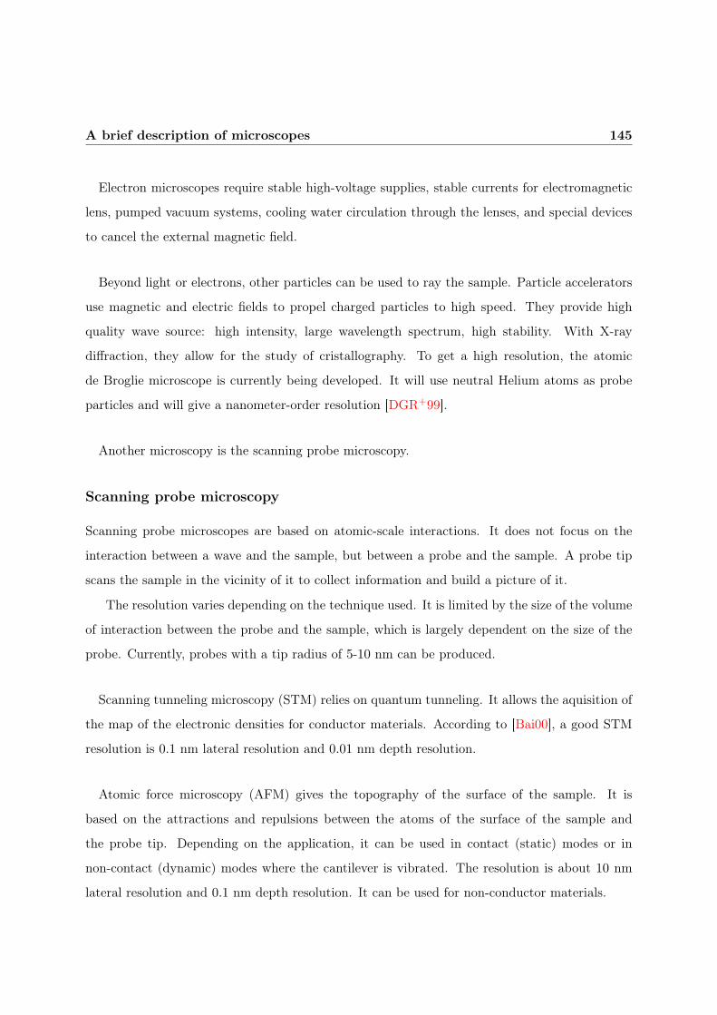
A brief description of microscopes 145
Electron microscopes require stable high-voltage supplies, stable currents for electromagnetic
lens, pumped vacuum systems, cooling water circulation through the lenses, and special devices
to cancel the external magnetic field.
Beyond light or electrons, other particles can be used to ray the sample. Particle accelerators
use magnetic and electric fields to propel charged particles to high speed. They provide high
quality wave source: high intensity, large wavelength spectrum, high stability. With X-ray
diffraction, they allow for the study of cristallography. To get a high resolution, the atomic
de Broglie microscope is currently being developed. It will use neutral Helium atoms as probe
particles and will give a nanometer-order resolution [DGR+99].
Another microscopy is the scanning probe microscopy.
Scanning probe microscopy
Scanning probe microscopes are based on atomic-scale interactions. It does not focus on the
interaction between a wave and the sample, but between a probe and the sample. A probe tip
scans the sample in the vicinity of it to collect information and build a picture of it.
The resolution varies depending on the technique used. It is limited by the size of the volume
of interaction between the probe and the sample, which is largely dependent on the size of the
probe. Currently, probes with a tip radius of 5-10 nm can be produced.
Scanning tunneling microscopy (STM) relies on quantum tunneling. It allows the aquisition of
the map of the electronic densities for conductor materials. According to [Bai00], a good STM
resolution is 0.1 nm lateral resolution and 0.01 nm depth resolution.
Atomic force microscopy (AFM) gives the topography of the surface of the sample. It is
based on the attractions and repulsions between the atoms of the surface of the sample and
the probe tip. Depending on the application, it can be used in contact (static) modes or in
non-contact (dynamic) modes where the cantilever is vibrated. The resolution is about 10 nm
lateral resolution and 0.1 nm depth resolution. It can be used for non-conductor materials.

146 Appendix A
Scanning near-field optical microscope collects evanescent waves at the vicinity of the sample
(at a distance much smaller than the wavelength of the light). With this technique, the critical
parameter is the size of the detector aperture. The resolutions are about 20 nm for lateral
directions and 2-5 nm for the vertical direction.

Appendix B
Periodic Table
The periodic table is a tabular presentation of the 118 known chemical elements. Although there
were precursors, the periodic table is generally credited to Mendeleev [Men69].
Elements are presented by increasing atomic number, the number of protons in the nucleus.
By definition, each element has a specific atomic number. For uncharged atoms, the number of
electrons is equal to the atomic number. Thus, provided the number and the nature of atoms
to be simulated, this table allows for the determination of the total number of electrons in the
system.
The horizontal rows are called periods. The vertical columns lump together elements with
similar properties e.g. alkali metals, halogens, noble gases. Therefore, the horizontal rows contain
some gaps.

148
Appendix
B
1H 2He
3Li 4Be 5B 6C 7N 8O 9F 10Ne
11Na 12Mg 13Al 14Si 15P 16S 17Cl 18Ar
19K 20Ca 21Sc 22Ti 23V 24Cr 25Mn 26Fe 27Co 28Ni 29Cu 30Zn 31Ga 32Ge 33As 34Se 35Br 36Kr
37Rb 38Sr 39Y 40Zr 41Nb 42Mo 43Tc 44Ru 45Rh 46Pd 47Ag 48Cd 49In 50Sn 51Sb 52Te 53I 54Xe
55Cs 56Ba 57La 72Hf 73Ta 74W 75Re 76Os 77Ir 78Pt 79Au 80Hg 81Tl 82Pb 83Bi 84Po 85At 86Rn
87Fr 88Ra 89Ac
58Ce 59Pr 60Nd 61Pm 62Sm 63Eu 64Gd 65Tb 66Dy 67Ho 68Er 69Tm 70Yb 71Lu
90Th 91Pa 92U 93Np 94Pu 95Am 96Cm 97Bk 98Cf 99Es 100Fm 101Md 102No 103Lw
Table B.1: Periodic table of the elements

Appendix C
Atomic units
Using the international system of units is cumbersome to describe the nanoscale quantities. It
is more convenient to employ the so-called atomic units system.
Two families of atomic units exist: the Hartree atomic units and the Rydberg atomic units,
which differ in the choice of the mass unit and the charge unit. In the Hartree system, the mass
unit and the charge unit are respectively the electron rest mass me and the elementary charge e.
In the Rydberg system, they are 2me ande√2. In this dissertation, we use only the Hartree
system.
Table C.1 specifies the physical constants chosen as the fundamental units in the Hartree
system.
Dimension Name Symbol Value in SI units
Mass Electron rest mass me 9, 110.10−31 kg
Charge Elementary charge e 1, 603.10−19 C
Angular momentum Reduced Planck’s constant ~ = h2π 1, 055.10−34 J.s
Electric constant Coulomb’s constant κ = 14πε0
8, 988.109 kg.m3.s−2.C−2
Table C.1: Fundamental units of the Hartree atomic system

150 Appendix C
We highlight that all the elementary quantities (length, time, mass, electric current, thermo-
dynamic temperature, amount of substance and luminous intensity) not have an atomic unit.
For example, for electromagnetic studies, the atomic units system is complemented by some SI
units or cgs units.
From the four fundamental atomic units, we can derive other units. Table C.2 mentions some
derived atomic units.
Dimension Name Symbol Expression Value in SI units
Length Bohr radius a04πε0~2
mee25, 292.10−11 m
Energy Hartree energy Ha ~2
mea20= me
(e2
4πε0~
)24, 360.10−18 J
Time ~
Eh2, 419.10−17 s
Electric field Eh
e.a05, 142.1011 V.m−1
Force Eh
a08, 239.10−8 N
Pressure Eh
a302, 942.1013 Pa
Table C.2: Derived units of the atomic system

Appendix D
Electron configurations of the atoms
Appendix B contains the periodic table, which gives the number of protons specific to each
chemical element. For uncharged systems, the number of electrons in the electronic cloud is equal
to the number of protons in the nucleus. Beyond the number of electrons, the key information is
the electron configuration, i.e. the distribution of the electrons in the spectrum of the one-electron
eigenmodes.
The electron configuration can be established by the Aufbau principle, also called the “building-
up” principle. This Appendix lists the electron configurations of the 94 atoms which occur
naturally on Earth.
Among all the electrons of the electronic cloud, the chemical properties are determined by
the valence electrons, i.e. the electrons related to the outermost modes far from the nucleus.
Therefore, atoms with the same valence configuration exhibit similar properties.

152 Appendix D
Element Z Electron Element Z Electron
Configuration Configuration
Hydrogen H 1 1s1 Cadmium Cd 48 [Kr] 5s2 4d10
Helium He 2 1s2 Indium In 49 [Kr] 5s2 4d10 5p1
Lithium Li 3 1s2 2s1 Tin Sn 50 [Kr] 5s2 4d10 5p2
Beryllium Be 4 1s2 2s2 Antimony Sb 51 [Kr] 5s2 4d10 5p3
Boron B 5 1s2 2s2 2p1 Tellurium Te 52 [Kr] 5s2 4d10 5p4
Carbon C 6 1s2 2s2 2p2 Iodine I 53 [Kr] 5s2 4d10 5p5
Nitrogen N 7 1s2 2s2 2p3 Xenon Xe 54 [Kr] 5s2 4d10 5p6
Oxygen O 8 1s2 2s2 2p4 Caesium Cs 55 [Xe] 6s1
Fluorine F 9 1s2 2s2 2p5 Barium Ba 56 [Xe] 6s2
Neon Ne 10 1s2 2s2 2p6 Lanthanum La 57 [Xe] 6s2 5d1
Sodium Na 11 1s2 2s2 2p6 3s1 Cerium Ce 58 [Xe] 6s2 4f1 5d1
Magnesium Mg 12 1s2 2s2 2p6 3s2 Praseodymium Pr 59 [Xe] 6s2 4f3
Aluminium Al 13 1s2 2s2 2p6 3s2 3p1 Neodymium Nd 60 [Xe] 6s2 4f4
Silicon Si 14 1s2 2s2 2p6 3s2 3p2 Promethium Pm 61 [Xe] 6s2 4f5
Phosphorus P 15 1s2 2s2 2p6 3s2 3p3 Samarium Sm 62 [Xe] 6s2 4f6
Sulfur S 16 1s2 2s2 2p6 3s2 3p4 Europium Eu 63 [Xe] 6s2 4f7
Chlorine Cl 17 1s2 2s2 2p6 3s2 3p5 Gadolinium Gd 64 [Xe] 6s2 4f7 5d1
Argon Ar 18 1s2 2s2 2p6 3s2 3p6 Terbium Tb 65 [Xe] 6s2 4f9
Potassium K 19 [Ar] 4s1 Dysprosium Dy 66 [Xe] 6s2 4f10
Calcium Ca 20 [Ar] 4s2 Holmium Ho 67 [Xe] 6s2 4f11
Scandium Sc 21 [Ar] 4s2 3d1 Erbium Er 68 [Xe] 6s2 4f12
Titanium Ti 22 [Ar] 4s2 3d2 Thulium Tm 69 [Xe] 6s2 4f13
Vanadium V 23 [Ar] 4s2 3d3 Ytterbium Yb 70 [Xe] 6s2 4f14
Chromium Cr 24 [Ar] 4s1 3d5 Lutetium Lu 71 [Xe] 6s2 4f14 5d1

Electron configurations of the atoms 153
Manganese Mn 25 [Ar] 4s2 3d5 Hafnium Hf 72 [Xe] 6s2 4f14 5d2
Iron Fe 26 [Ar] 4s2 3d6 Tantalum Ta 73 [Xe] 6s2 4f14 5d3
Cobalt Co 27 [Ar] 4s2 3d7 Tungsten W 74 [Xe] 6s2 4f14 5d4
Nickel Ni 28 [Ar] 4s2 3d10 Rhenium Re 75 [Xe] 6s2 4f14 5d5
or [Ar] 4s1 3d9
Copper Cu 29 [Ar] 4s1 3d10 Osmium Os 76 [Xe] 6s2 4f14 5d6
Zinc Zn 30 [Ar] 4s2 3d10 Iridium Ir 77 [Xe] 6s2 4f14 5d7
Gallium Ga 31 [Ar] 4s2 3d10 4p1 Platinum Pt 78 [Xe] 6s1 4f14 5d9
Germanium Ge 32 [Ar] 4s2 3d10 4p2 Gold Au 79 [Xe] 6s1 4f14 5d10
Arsenic As 33 [Ar] 4s2 3d10 4p3 Mercury Hg 80 [Xe] 6s2 4f14 5d10
Selenium Se 34 [Ar] 4s2 3d10 4p4 Thallium Tl 81 [Xe] 6s2 4f14 5d10 6p1
Bromine Br 35 [Ar] 4s2 3d10 4p5 Lead Pb 82 [Xe] 6s2 4f14 5d10 6p2
Krypton Kr 36 [Ar] 4s2 3d10 4p6 Bismuth Bi 83 [Xe] 6s2 4f14 5d10 6p3
Rubidium Rb 37 [Kr] 5s1 Polonium Po 84 [Xe] 6s2 4f14 5d10 6p4
Strontium Sr 38 [Kr] 5s2 Astatine At 85 [Xe] 6s2 4f14 5d10 6p5
Yttrium Y 39 [Kr] 5s2 4d1 Radon Rn 86 [Xe] 6s2 4f14 5d10 6p6
Zirconium Zr 40 [Kr] 5s2 4d2 Francium 87 Fr [Rn] 7s1
Niobium Nb 41 [Kr] 5s1 4d4 Radium Ra 88 [Rn] 7s2
Molybdenum Mo 42 [Kr] 5s1 4d5 Actinium Ac 89 [Rn] 7s2 6d1
Technetium Tc 43 [Kr] 5s2 4d5 Thorium Th 90 [Rn] 7s2 6d2
Ruthenium Ru 44 [Kr] 5s1 4d7 Protactinium Pa 91 [Rn] 7s2 5f2 6d1
Rhodium Rh 45 [Kr] 5s1 4d8 Uranium U 92 [Rn] 7s2 5f3 6d1
Palladium Pd 46 [Kr] 4d10 Neptunium Np 93 [Rn] 7s2 5f4 6d1
Silver Ag 47 [Kr] 5s1 4d10 Plutonium Pu 94 [Rn] 7s2 5f6

Appendix E
Quantum numbers
In classical mechanics, the characteristics of a material can range continously whereas quantum
mechanics provide the quantization of observable quantities. Quantum numbers describe any
quantum system by a discrete set of integers or half-integers. This Appendix describes briefly
these numbers, for complements we refer to [Hla97, AF05].
Each operator A that commutes with the Hamiltonian (i.e. satisfies the relation AH = HA)
can be associated with a quantum number. An electronic wave function in an atom can be
completely described by a set of four independent quantum numbers, but this set is not unique.
Among the different models, we present here the set proposed by the Hund-Mulliken molecular
orbital theory which describes electrons by the four quantum numbers n, l, m and ms.
The principal or first quantum number n labels the nth eigenvalue of Hamiltonian with the
contribution due to angular momentum left out. Therefore, it always have a positive integer
value.
The azimuthal quantum number l, also known as the angular quantum number or the second
quantum number gives the magnitude of the orbital angular momentum as: L2 = hl(l + 1). In
the literature, an eigenmode for which l = 0 is called a s orbital, in the case of l = 1, l = 2 or
l = 3, they are called respectively a p orbital, a d orbital or a f orbital.
The magnetic quantum number m yields the projection of the orbital angular momentum

156 Appendix E
along a specific axis Lz. The values of m range from −l to l with integer steps between them.
The spin projection quantum number ms gives the projection of the spin angular momentum
S along the specific axis: Sz = msh. For an electronic wave function, the values of ms can be
−12 or 1
2 .
According to Hund’s rules, two electrons can never have the same set of quantum numbers.

Appendix F
The weak form of the Hartree-Fock
system
This Appendix presents the calculation to get the weak form of the Hartree-Fock system from the
Schrödinger equation. For the sake of clarity, the calculation is detailed in the case of a system
comprising one nucleus with Z protons located in X, and two electrons located respectively in
x1 and x2. The two electrons are described by the wave function Ψe:
Ψe : x = (x1, x2) 7−→ Ψe (x)
R6 −→ C.
The eigenpair (Ψe, Ee) is solution of the Schrödinger problem (section 2.5):
1
2(∇xΨe,∇xδΨe) + ((Ven + Vee)Ψe, δΨe) = Ee (Ψe, δΨe) +
δEe
2[(Ψe,Ψe)− 1]
+ δλ[Ψe(xσ(1), xσ(2))− sg (σ)Ψe(x1, x2)
],
∀δΨe ∈ W, ∀δEe ∈ WEe , ∀δλ ∈ W
λ, (F.1)
where Ee appears as a Lagrange multiplier associated with the unit norm of Ψe. δEe and δλ are
two test Lagrange multipliers.
The Hartree-Fock method solves the Schrödinger equation in the space WHF . The wave
function Ψe is approximated by a Slater determinant ΨHFe built from two orthonormal one-

158 Appendix F
electron wave functions ϕ1 and ϕ2 defined in R3:
Ψe ∼ ΨHFe =
1√2
∣∣∣∣∣∣∣
ϕ1(x1) ϕ1(x2)
ϕ2(x1) ϕ2(x2)
∣∣∣∣∣∣∣
rR3 ϕ
∗1ϕ1 =
rR3 ϕ
∗2ϕ2 = 1
rR3 ϕ
∗1ϕ2 =
rR3 ϕ
∗2ϕ1 = 0
where
ϕ1 : x1 7→ ϕ1 (x1)
R3 → C
ϕ2 : x2 7→ ϕ2 (x2)
R3 → C.
(F.2)
The normality and anti-symmetry of the solution is ensured by the form of the Hartree-Fock trial
function. The orthonormalization of the one-electron wave functions is imposed by the Lagrange
multipliers Λ11, Λ22 and Λ12. We denote Φ =
ϕ1
ϕ2
and Λ =
Λ11 Λ12
Λ21 Λ22
. The Hartree-Fock
problem reads:
1
2
(∇xΨ
HFe ,∇xδΨ
HFe
)+((Ven + Vee)Ψ
HFe , δΨHF
e
)= δ
[
tr
[Λ
2·((w
R3Φ⊗ Φ
)
− I)]]
.
We express this problem as a function of the one-electron wave functions. The electronic
kinetic energy reads:
(∇xΨ
HFe ,∇xδΨ
HFe
)=(∇x1Ψ
HFe ,∇x1δΨ
HFe
)+(∇x2Ψ
HFe ,∇x2δΨ
HFe
)
where
(∇x1Ψ
HFe ,∇x1δΨ
HFe
)= (∇x1ϕ1 (x1)ϕ2 (x2)− ϕ1 (x2)∇x1ϕ2 (x1) ,∇x1δϕ1 (x1)ϕ2 (x2)
+∇x1ϕ1 (x1) δϕ2 (x2)− δϕ1 (x2)∇x1ϕ2 (x1)− ϕ1 (x2)∇x1δϕ2 (x1))(∇x1Ψ
HFe ,∇x1δΨ
HFe
)=
1
2(∇x1ϕ1 (x1) ,∇x1δϕ1 (x1)) ,
therefore
(∇xΨ
HFe ,∇xδΨ
HFe
)= (∇xΦ,∇xδΦ) .
Now, we focus on the interactions between the electrons and the nucleus:
(VenΨ
HFe , δΨHF
e
)=
( −Z|X − x1|
ΨHFe , δΨHF
e
)
+
( −Z|X − x2|
ΨHFe , δΨHF
e
)

The weak form of the Hartree-Fock system 159
where( −Z|X − x1|
ΨHFe , δΨHF
e
)
=
[ −Z2|X − x1|
(ϕ1 (x1)ϕ2 (x2)− ϕ1 (x2)ϕ2 (x1)) ,
δϕ1 (x1)ϕ2 (x2) + ϕ1 (x1) δϕ2 (x2)− δϕ1 (x2)ϕ2 (x1)− ϕ1 (x2) δϕ2 (x1)
]
=
( −Z2|X − x1|
ϕ1, δϕ1
)
+
( −Z2|X − x1|
ϕ2, δϕ2
)
so(VenΨ
HFe , δΨHF
e
)=
( −Z|X − x1|
Φ, δΦ
)
+
( −Z|X − x2|
Φ, δΦ
)
.
Finally, we look into the interaction between electrons:
(VeeΨ
HFe , δΨHF
e
)=
(1
|x1 − x2|ΨHF
e , δΨHFe
)
=
(1
2|x1 − x2|(ϕ1 (x1)ϕ2 (x2)− ϕ1 (x2)ϕ2 (x1)) ,
δϕ1 (x1)ϕ2 (x2) + ϕ1 (x1) δϕ2 (x2)− δϕ1 (x2)ϕ2 (x1)− ϕ1 (x2) δϕ2 (x1)
)
=
( |ϕ1|2|x1 − x2|
ϕ2, δϕ2
)
+
( |ϕ2|2|x1 − x2|
ϕ1, δϕ1
)
−(
ϕ1ϕ2
|x1 − x2|ϕ2, δϕ1
)
−(
ϕ1ϕ2
|x1 − x2|ϕ1, δϕ2
)
= ((tr (G) I −G) Φ, δΦ) .
The orthonormalization of the one-electron wave functions by the Lagrange multipliers leads to:
δ[tr(Λ2 ·((r
R3 Φ⊗ Φ)− I))]
= tr[δΛ2 ·(r
R3 (Φ⊗ Φ)− I)]
+ tr[Λ2 ·(r
R3 (δΦ⊗ Φ) +rR3 (Φ⊗ δΦ)
)]
= tr[δΛ2 ·(r
R3 (Φ⊗ Φ)− I)]
+ tr[Λ ·
rR3 (Φ⊗ δΦ)
]
= tr[δΛ2 ·(r
R3 (Φ⊗ Φ)− I)]
+ (ΛΦ, δΦ) .
Therefore, the weak form of the Hartree-Fock problem reads:
(
−1
2∇Φ,∇δΦ
)
+ ((Ven + tr (G) I −G) Φ, δΦ) = (ΛΦ, δΦ) + tr[
δΛ ·(
I −w
R3Φ⊗ Φ∗
)]
,
∀δΦ ∈ WΦ, ∀δΛ ∈ W
Λ. (F.3)


Appendix G
Setting up the Hartree-Fock system
This Appendix details the calculation to obtain the strong form of the Hartree-Fock system from
the Schrödinger equation. For the sake of clarity, the calculation is exposed for the case of a
system composed of one nucleus of Z protons located in X and two electrons located respectively
in x1 and x2. The two electrons are described by a unique wave function Ψe:
Ψe : x = (x1, x2) 7−→ Ψe (x)
R6 −→ C
which is solution of the following system:
−1
2∆xΨe +
( −Z|X − x1|
+−Z
|X − x2|+
1
|x1 − x2|
)
Ψe = EeΨe,
rR6 |Ψe|2dx = 1,
Ψe(xσ(1), xσ(2)) = sg (σ)Ψe(x1, x2).
(G.1)
The Hartree-Fock method solves the Schrödinger equation in a reduced space WHF . The
Hartree-Fock strategy approximates the wave function Ψe by a Slater determinant ΨHFe built
from two orthonormal one-electron wave functions ϕ1 and ϕ2 defined in R3:
Ψe ∼ ΨHFe =
1√2
∣∣∣∣∣∣∣
ϕ1(x1) ϕ1(x2)
ϕ2(x1) ϕ2(x2)
∣∣∣∣∣∣∣
rR3 ϕ
∗1ϕ1 =
rR3 ϕ
∗2ϕ2 = 1
rR3 ϕ
∗1ϕ2 =
rR3 ϕ
∗2ϕ1 = 0
where
ϕ1 : x1 7→ ϕ1 (x1)
R3 → C
ϕ2 : x2 7→ ϕ2 (x2)
R3 → C.
(G.2)

162 Appendix G
By choosing a Hartree-Fock trial function, the conditions of normality and anti-symmetry of the
wave function Ψe are automatically satisfied.
The ground-state eigenpair (ΨHFe , EHF
e ) minimizes the electronic energy:
EHFe =
(
−1
2∆xΨe +
( −Z|X − x1|
+−Z
|X − x2|+
1
|x1 − x2|
)
ΨHFe ,ΨHF
e
)
.
We express this energy as a function of the one-electron wave functions:
EHFe =
(
−1
2∆x
1√2(ϕ1(x1)ϕ2(x2)− ϕ2(x1)ϕ1(x2)) ,
1√2(ϕ1(x1)ϕ2(x2)− ϕ2(x1)ϕ1(x2))
)
+
( −Z|X − x1|
1√2(ϕ1(x1)ϕ2(x2)− ϕ2(x1)ϕ1(x2)) ,
1√2(ϕ1(x1)ϕ2(x2)− ϕ2(x1)ϕ1(x2))
)
+
( −Z|X − x2|
1√2(ϕ1(x1)ϕ2(x2)− ϕ2(x1)ϕ1(x2)) ,
1√2(ϕ1(x1)ϕ2(x2)− ϕ2(x1)ϕ1(x2))
)
+
(1
|x1 − x2|1√2(ϕ1(x1)ϕ2(x2)− ϕ2(x1)ϕ1(x2)) ,
1√2(ϕ1(x1)ϕ2(x2)− ϕ2(x1)ϕ1(x2))
)
Using the orthonormality of the one-electron wave functions, we can express simply the electronic
energy. The Hartree-Fock problem reads:
min
EHFe = −
(1
2∆x1ϕ1(x1), ϕ1(x1)
)
−(1
2∆x2ϕ2(x2), ϕ2(x2)
)
+
( −Z|X − x1|
ϕ1(x1), ϕ1 (x1)
)
+
( −Z|X − x2|
ϕ2(x2), ϕ2 (x2)
)
+
((ϕ1 (x1)
|x1 − x2|, ϕ1(x1)
)
ϕ2(x2), ϕ2(x2)
)
−((
ϕ1 (x1)
|x1 − x2|, ϕ2(x1)
)
ϕ1(x2), ϕ2(x2)
)
,
1 = (ϕ1, ϕ1) = (ϕ2, ϕ2) ,
0 = (ϕ1, ϕ2) = (ϕ2, ϕ1) .
We solve this problem with the Euler-Lagrange equations, and impose the orthonormalization
constraint using the Lagrange multipliers Λ11, Λ12 and Λ22:
L (ϕ1, ϕ2,Λ11,Λ12,Λ22) = EHFe + Λ11
(
1−w
R3ϕ1ϕ
∗1
)
+ Λ12
w
R3ϕ∗1ϕ2
+ Λ12
w
R3ϕ∗2ϕ1 + Λ22
(
1−w
R3ϕ∗2ϕ2
)
. (G.3)
Minimizing this Lagrangian, we get:
dL =∂L∂ϕ1
dϕ1 +∂L∂ϕ2
dϕ2 +∂L∂Λ11
dΛ11 +∂L∂Λ22
dΛ22 +∂L∂Λ12
dΛ12 = 0,
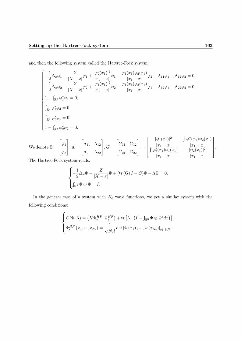
Setting up the Hartree-Fock system 163
and then the following system called the Hartree-Fock system:
−1
2∆xϕ1 −
Z
|X − x|ϕ1 +|ϕ2(x1)|2|x1 − x| ϕ1 −
ϕ1(x1)ϕ2(x1)
|x1 − x| ϕ2 − Λ11ϕ1 − Λ12ϕ2 = 0,
−1
2∆xϕ2 −
Z
|X − x|ϕ2 +|ϕ1(x1)|2|x1 − x| ϕ2 −
ϕ1(x1)ϕ2(x1)
|x1 − x| ϕ1 − Λ12ϕ1 − Λ22ϕ2 = 0,
1−rR3 ϕ
∗1ϕ1 = 0,
rR3 ϕ
∗1ϕ2 = 0,
rR3 ϕ
∗2ϕ1 = 0,
1−rR3 ϕ
∗2ϕ2 = 0.
We denote Φ =
ϕ1
ϕ2
, Λ =
Λ11 Λ12
Λ21 Λ22
, G =
G11 G12
G21 G22
=
|ϕ1(x1)|2|x1 − x|
rϕ∗1(x1)ϕ2(x1)
|x1 − x|rϕ∗2(x1)ϕ1(x1)
|x1 − x||ϕ2(x1)|2|x1 − x|
.
The Hartree-Fock system reads:
−1
2∆xΦ− Z
|X − x|Φ+ (tr (G) I −G)Φ− ΛΦ = 0,
rR3 Φ⊗ Φ = I.
In the general case of a system with Ne wave functions, we get a similar system with the
following conditions:
L (Φ,Λ) =(HΨHF
e ,ΨHFe
)+ tr
[Λ ·(I −
rR3 Φ⊗ Φ∗dx
)],
ΨHFe (x1, ..., xNe) =
1√Ne!
det [Φ (x1) , ...,Φ (xNe)]i∈[1;Ne].

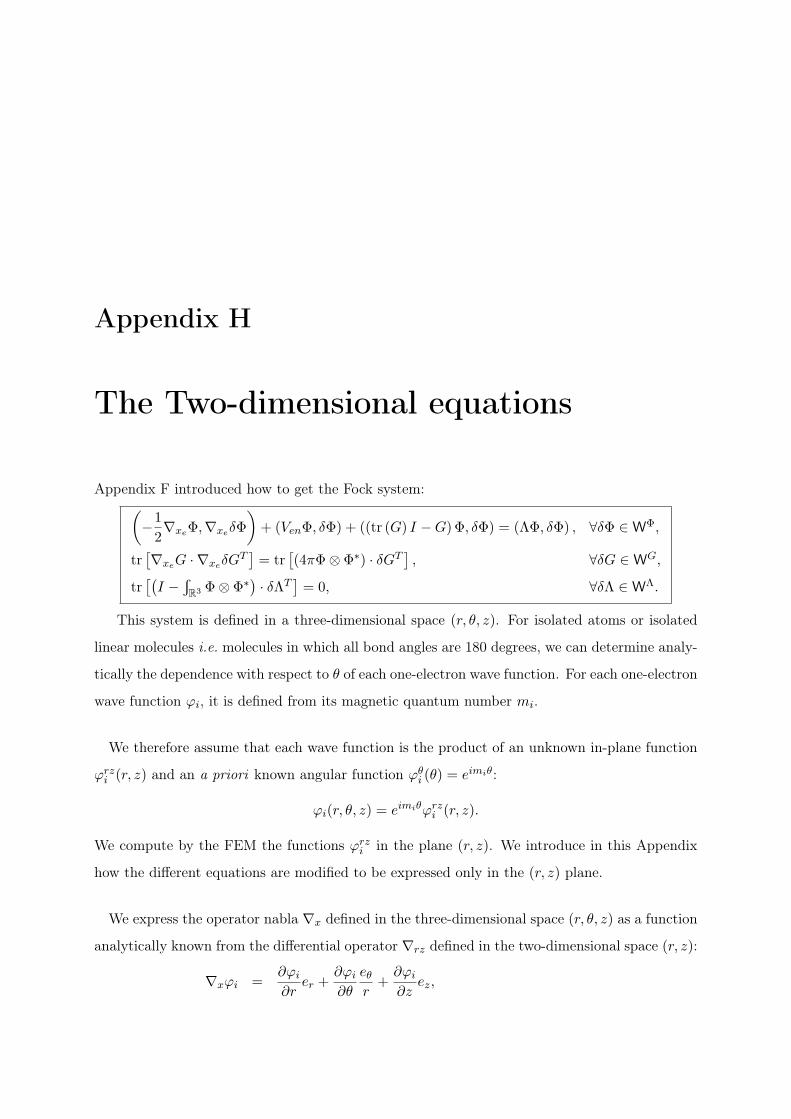
Appendix H
The Two-dimensional equations
Appendix F introduced how to get the Fock system:(
−1
2∇xeΦ,∇xeδΦ
)
+ (VenΦ, δΦ) + ((tr (G) I −G) Φ, δΦ) = (ΛΦ, δΦ) , ∀δΦ ∈ WΦ,
tr[∇xeG · ∇xeδG
T]= tr
[(4πΦ⊗ Φ∗) · δGT
], ∀δG ∈ W
G,
tr[(I −
rR3 Φ⊗ Φ∗
)· δΛT
]= 0, ∀δΛ ∈ W
Λ.
This system is defined in a three-dimensional space (r, θ, z). For isolated atoms or isolated
linear molecules i.e. molecules in which all bond angles are 180 degrees, we can determine analy-
tically the dependence with respect to θ of each one-electron wave function. For each one-electron
wave function ϕi, it is defined from its magnetic quantum number mi.
We therefore assume that each wave function is the product of an unknown in-plane function
ϕrzi (r, z) and an a priori known angular function ϕθ
i (θ) = eimiθ:
ϕi(r, θ, z) = eimiθϕrzi (r, z).
We compute by the FEM the functions ϕrzi in the plane (r, z). We introduce in this Appendix
how the different equations are modified to be expressed only in the (r, z) plane.
We express the operator nabla ∇x defined in the three-dimensional space (r, θ, z) as a function
analytically known from the differential operator ∇rz defined in the two-dimensional space (r, z):
∇xϕi =∂ϕi
∂rer +
∂ϕi
∂θ
eθ
r+∂ϕi
∂zez,
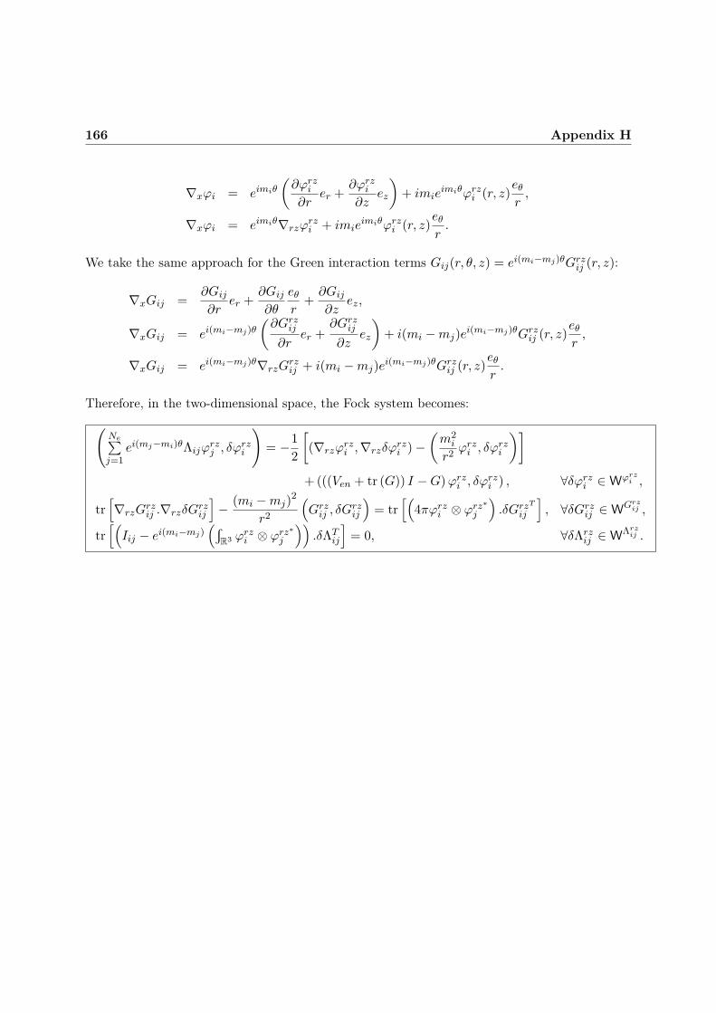
166 Appendix H
∇xϕi = eimiθ
(∂ϕrz
i
∂rer +
∂ϕrzi
∂zez
)
+ imieimiθϕrz
i (r, z)eθ
r,
∇xϕi = eimiθ∇rzϕrzi + imie
imiθϕrzi (r, z)
eθ
r.
We take the same approach for the Green interaction terms Gij(r, θ, z) = ei(mi−mj)θGrzij (r, z):
∇xGij =∂Gij
∂rer +
∂Gij
∂θ
eθ
r+∂Gij
∂zez,
∇xGij = ei(mi−mj)θ
(∂Grz
ij
∂rer +
∂Grzij
∂zez
)
+ i(mi −mj)ei(mi−mj)θGrz
ij (r, z)eθ
r,
∇xGij = ei(mi−mj)θ∇rzGrzij + i(mi −mj)e
i(mi−mj)θGrzij (r, z)
eθ
r.
Therefore, in the two-dimensional space, the Fock system becomes:
(Ne∑
j=1ei(mj−mi)θΛijϕ
rzj , δϕ
rzi
)
= −1
2
[
(∇rzϕrzi ,∇rzδϕ
rzi )−
(m2
i
r2ϕrzi , δϕ
rzi
)]
+(((Ven + tr (G)) I −G)ϕrzi , δϕ
rzi ) , ∀δϕrz
i ∈ Wϕrzi ,
tr[
∇rzGrzij .∇rzδG
rzij
]
− (mi −mj)2
r2
(
Grzij , δG
rzij
)
= tr[(
4πϕrzi ⊗ ϕrz∗
j
)
.δGrzTij
]
, ∀δGrzij ∈ W
Grzij ,
tr[(
Iij − ei(mi−mj)(r
R3 ϕrzi ⊗ ϕrz∗
j
))
.δΛTij
]
= 0, ∀δΛrzij ∈ W
Λrzij .

Appendix I
Magnetic properties
We can benefit from quantum computations to estimate magnetic properties such as the magnetic
moment and the magnetizability [Sla51, RSL63, AF05]. We derive them from the total energy
E when the Schrödinger equation takes the magnetic field into account. The magnetic moment
m and the magnetizability tensor ξ can be defined respectively as the opposite of the derivative
of the energy with respect to the magnetic field B at the first order and at the second order:
m = −∂E∂B
, (I.1)
ξ = − ∂2E
∂B∂B. (I.2)
The magnetic potential of a system under the application of an external magnetic field B
reads [NLK86]:
V mage (xk) = e i (∇xk
. ∧B)xk, (I.3)
V magn (Xj) = e i Zj (∇xk
. ∧B)Xj . (I.4)
From equation (1.33), a perturbation of the magnetic field δB leads to a perturbation of the
potential δVe = e i (∇xk. ∧ δB)xk and a perturbation of the electronic energy:
δEe = ((e i (∇xk. ∧ δB)xk)Ψe,Ψe) . (I.5)
Thus, the electronic magnetic dipole moment denoted by me and defined by equation (1.4) reads
me = − ((e i (∇xk. ∧ 1)xk)Ψe,Ψe) . (I.6)

168 Appendix I
The magnetic dipole moment describes the torque that a magnetic field can exert on the system
and the force that the system can exert on electric currents. It is expressed in A.m2 or in J.T−1 in
the SI system. Considering the Hartree-Fock approximation and the nuclei as particles without
speed, the magnetic moment can be expressed as follows:
mHF = − ((e i (∇xk. ∧ 1)xk) Φ,Φ) . (I.7)
Using the configuration interaction approximation, it yields that:
mCI = −Nd∑
A=1
Nd∑
B=1
αAαB
((e i (∇xk
. ∧ 1)xk) ΦA,ΦB
). (I.8)
The magnetizability tensor ξ characterizes the ability of a system to be magnetized by any ex-
ternal magnetic field. It is expressed in m2.A2.s2.kg−1 or in J.T−2 in the SI system, or in e2.a20.m−1e
in the atomic system. From equation (4.11), we establish:
δ2E =((e i(∇xk
. ∧ δ2B)xk)Ψe,Ψe
)+ 2 ((e i (∇xk
. ∧ δB)xk)⊗ δΨe,Ψe) (I.9)
therefore the magnetizability tensor defined by equation (I.2) reads:
ξ = − ((e i (∇xk. ∧ 1)xk)Ψe,Ψe)− 2
(
(e i (∇xk. ∧ 1)xk)⊗
δΨe
δB,Ψe
)
. (I.10)
Applying the Hartree-Fock model, it yields that:
ξHF = − ((e i (∇xk. ∧ 1)xk) Φ,Φ)− 2
(
(e i (∇xk. ∧ 1)xk)⊗
δΦ
δB,Φ
)
. (I.11)
With the configuration interaction approximation, it reads:
ξCI = −Nd∑
A=1
Nd∑
B=1
αAαB
[((e i (∇xk
. ∧ 1)xk) ΦA,ΦB
)+ 2
(
(e i (∇xk. ∧ 1)xk)⊗
δΦA
δB,ΦB
)]
.
(I.12)

Appendix J
Crystals: The Bloch theorem
In Chapter 4, we presented numerical results for isolated systems. However, most systems
interact with their surroundings. For instance, atoms in crystals present periodic interactions
with neighboring atoms. This Appendix focuses on the Bloch theorem which is applied to model
and analyze crystal structures.
The periodic atomic arrangement in crystals
A crystal is a solid material, whose constituent atoms are arranged in an orderly repeating
pattern extending in all three spatial dimensions. For example, Figure J.1 represents the LiH
crystal, which is composed of lithium and hydrogen atoms perfectly ordered.
Li atom
H atom
Figure J.1: Scheme of a perfect LiH crystal

170 Appendix J
|a1| = |a2| = |a3|α = β = γ = 90°
(a) simple cubic
|a1| = |a2| = |a3|α = β = γ = 90°
(b) body-centered cubic
|a1| = |a2| = |a3|α = β = γ = 90°
(c) face-centered cubic
|a1| = |a2| 6= |a3|α = β = γ = 90°
(d) simpletetragonal
|a1| = |a2| 6= |a3|α = β = γ = 90°
(e) body-centeredtetragonal
|a1| 6= |a2| 6= |a3|α = β = 90°γ 6= 120°
(f) simple
monoclinic
|a1| 6= |a2| 6= |a3|α = β = 90°γ 6= 120°
(g) base-centered
monoclinic
|a1| 6= |a2| 6= |a3|α = β = γ = 90°
(h) simpleorthorombic
|a1| 6= |a2| 6= |a3|α = β = γ = 90°
(i) base-centeredorthorombic
|a1| 6= |a2| 6= |a3|α = β = γ = 90°
(j) body-centeredorthorombic
|a1| 6= |a2| 6= |a3|α = β = γ = 90°
(k) face-centeredorthorombic
|a1| 6= |a2| 6= |a3|α 6= β 6= γ 6= 90°
(l) triclinic
|a1| = |a2| = |a3|α = β = γ 6= 90°
(m) rhombohedral
|a1| = |a2| 6= |a3|α = β = 90°γ = 120°
(n) hexagonal
Figure J.2: The 14 three-dimensional Bravais lattices (parallelograms whose lengths of side are
|a1|, |a2| and |a3|, and the angles between the different sides α, β and γ)

Crystals: The Bloch theorem 171
The periodicity of the lattice is described by a geometrical arrangement and a chemical
arrangement.
The geometrical arrangement is defined by a Bravais lattice [Bra50], which is a regular distri-
bution of points in the space respecting the periodicity of the crystal. Provided the positions X0
of the nuclei of the atoms of one cell of the crystal, the positions Xn of the other nuclei of the
crystal lattice can be obtained by translation of the first cell:
Xn = X0 + niai (J.1)
with ai the direction vectors and ni the number of cells in the direction of ai. The parameters
of the lattice are the lengths |ai| of the primitive vectors and the angles formed by them: α, β
and γ. For example, Figure J.3 represents the cubic Bravais lattice of the LiH crystal.
a1 = a2 = a3 = 2, 042.10−10m
α = β = γ = 90°
Figure J.3: Bravais lattice of the LiH crystal
The Bravais lattice can be considered as a vector space where the scalars ni are only integers.
The basis of the Bravais lattice is a set of vectors ai, which are linearly independent in R3. This
basis is not unique, but its volume is unique. The fundamental space is constituted by the points
whose coordinates ni belongs to [0, 1[. Generally, it is called the primitive cell.
We can classify lattices with respect to their symmetry group, which describes rotations and
translations that do not disturb the lattice. Therefore, the number of different lattices is infinite
but the number of types of lattices is finite. In a one-dimensional space, only one type of lattice
exists. Five different types of lattice exist in a two-dimensional space and fourteen different types
in a three-dimensional space. They are represented on Figure J.2.

172 Appendix J
Because a crystal can be composed of different types of atoms, the distribution of points is not
sufficient to characterize the whole structure. It is necessary to clarify the chemical arrangement
by the description of a periodic cell. The whole structure can be built by translation operations
of this cell. Therefore, the cell represented on Figure J.4(a) can not be considered as a periodic
cell whereas the cells of Figure J.4(b) and Figure J.4(c) are acceptable. The cell represented on
Figure J.4(c) is the elementary cell also called the Wigner-Seitz cell or the Dirichlet zone.
Li atomH atom
(a) a non-periodic cell (b) a periodic cell (c) the elementary cell
Figure J.4: Different cells of the LiH crystal
Let us consider the electrons of a perfect infinite crystal, the structure is perfectly periodic,
but not the wave function of the system. Lots of efforts could be saved by reducing the FEM
domain from the entire periodic crystal to a primitive cell by applying the Bloch theorem.
The Bloch theorem
Numerical computations aim at taking advantage of the periodicity of the lattice to reduce
computational costs. The Bloch transformation was introduced in 1928 [Blo28], and it is tradi-
tionnally used in the context of solid state physics [AF05]. Nevertheless, this approach is also
appealing to analyze other periodic structures e.g. honeycombs [ACV98, TTAS11].
The perfect crystal is a periodic strucure Ω of space dimension Nc. Let us define a primitive
cell Q0 and a set of basis vectors aii∈[1;Nc], called direct cell basis, such that the entire structure

Crystals: The Bloch theorem 173
Ω can be reconstituted by repeating the primitive cell along the three directions of the direct cell
basis. The reciprocal cell Q∗0, called the first Brillouin zone [Bri53] and the reciprocal cell basis
a∗i i∈[1;Nc]are defined as dual to Q0 and aii∈[1;Nc]
, and satisfy:
a∗i .aj
|ai| |aj |= δij
|Q0| |Q∗0| = 1,
(J.2)
where δij stands for the Kronecker delta, and |Q0| and |Q∗0| are respectively the volumes of the
elementary Wigner-Seitz cell and the volume of the first Brillouin cell.
For any non-periodic function Ψe (x) defined on ΩNe , the Bloch theorem states that, for each
wave vector k of the first Brillouin zone, the Bloch wave functions Ψke (x, k) are some periodic
functions with the same periodicity as the crystal Ω, which are defined as:
Ψke : (x, k) 7−→ Ψk
e (x, k) =Nc∑
i=1Ψe (x+ niai) exp
i(k,x+niai)
ΩNe ×Q∗Ne
0 −→ C,
(J.3)
from the non-periodic function Ψe(x) :
Ψe : x 7−→ Ψe (x)
ΩNe −→ C,
with ni ∈ Z the number of cells in the direction of the vector ai.
The inverse Bloch transformation provides the value of the wave function Ψe at any point x
by integrating the Bloch wave functions Ψke (x, k) over the first Brillouin zone Q∗
0:
Ψe (x) =1
|Q∗0|
w
Q∗
0
Ψke (x, k) exp
−i(k,x) dk. (J.4)
Thus, by virtue of the Bloch theorem, any non-periodic wave function in a periodic crystal
can be decomposed into Bloch wave functions Ψke that are periodic with periods ai in the direct
space. The strategy to solve a crystal can be summed up by Figure J.5.

174 Appendix J
Direct Space
Known periodic VUnknown unperiodic Ψe
Reciprocal Space
Known periodic V = V
Unknown periodic Ψke
Solution ΨkeSolution Ψe
➋ Solving
➊ Ψke (x, k) =
3∑
i=1Ψe (x+ niai) exp
i(k,x+niai)
➌ Ψe (x) =1
|Q⋆0|
rQ⋆
0Ψk
e (x, k) exp−i(k,x) dk
Figure J.5: Modeling a perfect crystal
Let us suppose a three-dimensional perfectly periodic crystal, the crystal wave function is
defined in R3Ne and the Bloch function is defined from a 6Ne-dimensional space, which is the
sum of the x-space and the k-space. The Schrödinger equation is solved in this 6Ne-dimensional
space to provide the function Ψke(x, k). From which, we build a posteriori the solution Ψe(x).
Therefore, the problem can be solved only on the elementary cell in the direct space.
To obtain the solution of the problem not only in the elementary cell but also in the whole
crystal, we use the periodicity properties of the Bloch functions:
Ψe (x+ ni.ai) =1
|Q∗0|
w
Q∗
0
Ψke (x, k) exp
−i(k,x+ni.ai) dk. (J.5)
The periodic problem
From the Schrödinger problem (equation 2.5), we deduce that the periodic wave function Ψe
satisfies:
1
2
(
∇xΨke ,∇xδΨ
ke
)
+
(
i k∇xΨke +
1
2|k|2Ψk
e + VeΨke , δΨ
ke
)
= Eke
(
Ψke , δΨ
ke
)
+δEk
e
2
[(
Ψke , Ψ
ke
)
− 1]
+ δλk[
Ψke(xσ(1), . . . , xσ(Ne))− sg (σ) Ψk
e(x1, . . . , xNe)]
,
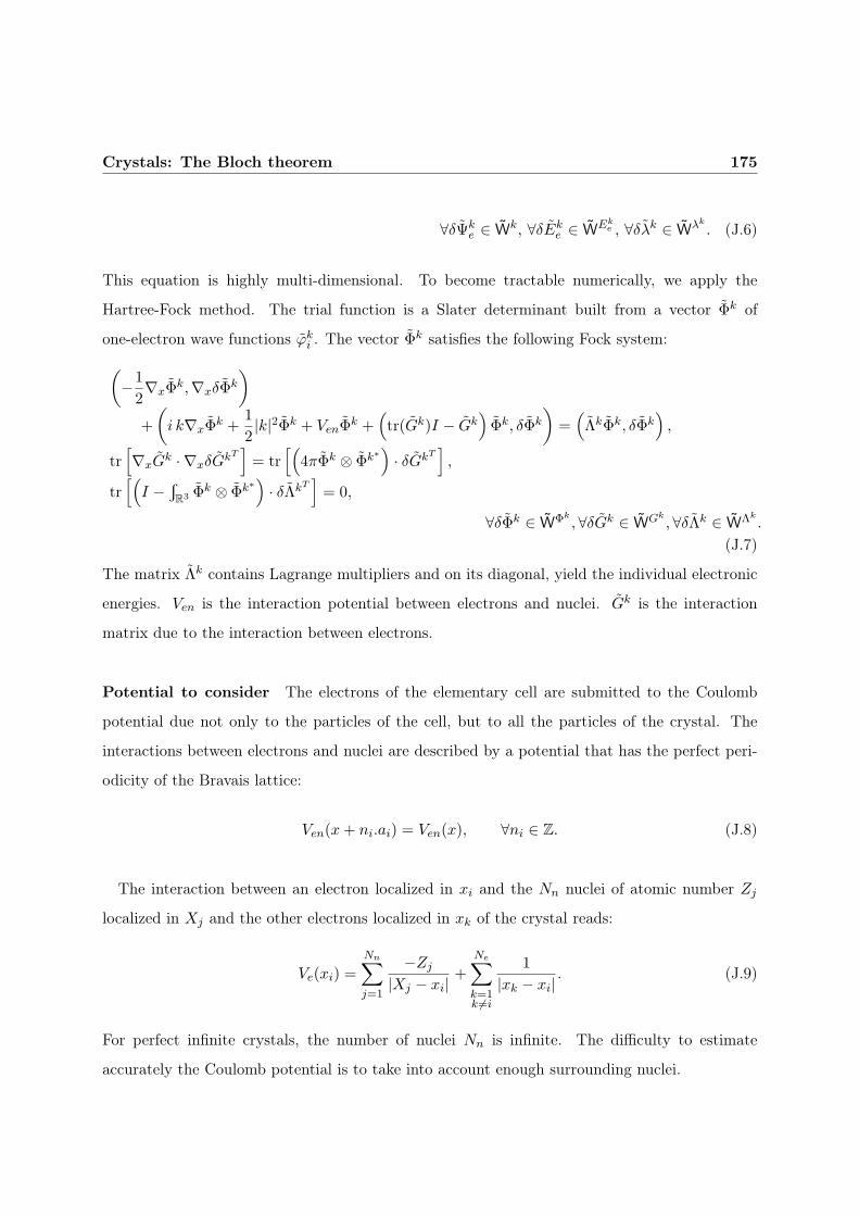
Crystals: The Bloch theorem 175
∀δΨke ∈ W
k, ∀δEke ∈ W
Eke , ∀δλk ∈ W
λk
. (J.6)
This equation is highly multi-dimensional. To become tractable numerically, we apply the
Hartree-Fock method. The trial function is a Slater determinant built from a vector Φk of
one-electron wave functions ϕki . The vector Φk satisfies the following Fock system:
(
−1
2∇xΦ
k,∇xδΦk
)
+
(
i k∇xΦk +
1
2|k|2Φk + VenΦ
k +(
tr(Gk)I − Gk)
Φk, δΦk
)
=(
ΛkΦk, δΦk)
,
tr[
∇xGk · ∇xδG
kT]
= tr[(
4πΦk ⊗ Φk∗)
· δGkT]
,
tr[(
I −rR3 Φ
k ⊗ Φk∗)
· δΛkT]
= 0,
∀δΦk ∈ WΦk, ∀δGk ∈ W
Gk, ∀δΛk ∈ W
Λk.
(J.7)
The matrix Λk contains Lagrange multipliers and on its diagonal, yield the individual electronic
energies. Ven is the interaction potential between electrons and nuclei. Gk is the interaction
matrix due to the interaction between electrons.
Potential to consider The electrons of the elementary cell are submitted to the Coulomb
potential due not only to the particles of the cell, but to all the particles of the crystal. The
interactions between electrons and nuclei are described by a potential that has the perfect peri-
odicity of the Bravais lattice:
Ven(x+ ni.ai) = Ven(x), ∀ni ∈ Z. (J.8)
The interaction between an electron localized in xi and the Nn nuclei of atomic number Zj
localized in Xj and the other electrons localized in xk of the crystal reads:
Ve(xi) =
Nn∑
j=1
−Zj
|Xj − xi|+
Ne∑
k=1k 6=i
1
|xk − xi|. (J.9)
For perfect infinite crystals, the number of nuclei Nn is infinite. The difficulty to estimate
accurately the Coulomb potential is to take into account enough surrounding nuclei.

176 Appendix J
Many works have been published on the methods to estimate the Coulomb potential in a
periodic structure [DPRS83]. According to [YDP93], it is essential to take into account long-
range electrostatic interactions. Truncated list methods (direct truncation and “twin-range”
cutoff methods) appear as poor methods. Ewald [Ewa21] proposes to consider the space as
repeating unit cells; details about the Ewald sums are provided in [TJ96, DPLP99]. Darden et
al. [DYP93] compute these sums by a fast N × lg (N) algorithm. Another approach is multipole
calculations. The space is divided into cells, and each cell is represented by a multipole moment
series: charges, dipoles, quadrupoles, octopoles,. . . This method becomes faster than the exact
algorithm when the number of atoms exceeds 300 [DKG92].
The number of eigenmodes is infinite, whereas the electronic density in the crystal is finite.
All the modes cannot be occupied. The occupied modes are determined by computing the Fermi
energy.
The Fermi energy
At 0 K, the energy of the system is the minimum of the energy functional that can admit an
electronic density matching the number of electrons on the elementary cell. This energy is called
the Fermi energy EF :
EF = minEe
w Ee
−∞ρ (Ee) dEe = Ne
. (J.10)
Electrons are fermions so they satisfy the Fermi-Dirac distribution µT (x) =1
1 + exp−x/kBT
[Fer26, Dir26]. The electronic density reads:
ρ(Ee) =2
|Ω|∑
i
w
Q∗
0
µ′T
(
Ee − Ekei (k)
)
dk, (J.11)
where the factor 2 is used considering a RHF approach. Ekei is the spectrum of eigenvalues, whose
values depend on the wave number k.
ρ(Ee) =2
|Q∗0|∑
i
w
Q∗
0
H ′(
Ee − Ekei (k)
)
dk (J.12)

Crystals: The Bloch theorem 177
where H is the Heaviside function defined by:
H(x) =
0, x < 0,
1, x > 0.
(J.13)
The derivative of this function is a Dirac mass at 0 that we denote δ.
ρ(Ee) =2
|Q∗0|∑
i
w
Q∗
0
δ(
Ee − Ekei (k)
)
dk (J.14)
For insulators at the equilibrium state, the surfaces Ekei (k) have dedicated rays and do not
cross the focus of other eigenvalues. Therefore, Ne
2 eigenmodes are fully occupied, the other ones
are void. In case of metals, a value Ee can match several eigenmodes, the determination of the
Fermi energy is a more delicate problem.
For instance, provided the band structure of a one-dimensional crystal illustrated on Figu-
re J.6, if there are two electrons per cell, only the first eigenmode is doubly occupied. Accordingly,
this system is an insulator. If there were three electrons per cell, the first mode is doubly occupied,
and the second and third eigenmodes would be both partially occupied. The crystal would be a
metal.
Eke1
Eke2
Eke3
Eke4
Ekei
k
Ekei
Figure J.6: The band structure of a one-dimensional crystal [Bla00]

178 Appendix J
Integration over the Brillouin zone
Once the periodic problem has been solved, the solution Φ (x) is built by integrating the Bloch
functions Φk (x, k) over the Brillouin zone.
To reduce the calculation time, for sufficiently smooth functions, it is possible to perform
the integration by estimating the function only in a carefully selected set of a few points in
the Brillouin zone called special points [Dal96]. Several sets of special points exist depending
on the Bravais lattice and the group symmetry [BSW36]. Historically, the use of the special
points was introduced by Baldereschi in 1973. He showed in [Bal73] that the computation of
the charge density of semiconductors could be performed by using a single point. Chadi and
Cohen [CC73a, CC73b] set up a procedure to generate special-point sets, and proposed sets for
the cubic and hexagonal lattices. Monkhorst and Park [MP76] introduced a more systematic
strategy based on equally spaced points. The application of the special-point method to metals
requires particular care, Methfessel and Paxton deal with this particular case in [MP89].


Abstract
Since performances of experimental and numerical tools have been largely improved, mechanics
of materials can explore smaller and smaller scales. Thus, a better comprehension, or even a
prediction, of local phenomena associated with macroscopic deformations are hoped. This disser-
tation focuses on the smallest scale involved in mechanical behavior of materials, i.e. interactions
between nuclei due to electrons behavior and especially to valence electrons. The originality of
this work is setting up the finite element method as numerical tool to solve this problem. This
approach largely used to solve structural mechanics problems provides powerful numerical tools
to tackle electronic structures. The Hartree-Fock and post-Hartree-Fock models are employed,
and mechanical properties of electronic structures are estimated. These estimates are based on
a set of approximations of both model and numerical origins. Error estimates are proposed to
analyze the accuracy of the results.
Résumé
Grâce à l’amélioration des performances des outils expérimentaux et numériques, la mécanique
des matériaux peut explorer des échelles de plus en plus fines. Une meilleure compréhension,
voire une prédiction, des phénomènes locaux mis en jeu est alors espérée. Cette thèse s’intéresse
à la plus petite échelle impliquée dans le comportement mécanique des matériaux, c.-à-d. les
interactions entre noyaux dues au comportement des électrons, et notamment des électrons de
valence. L’originalité de ce travail est dans la mise en place des éléments finis comme outil
numérique de résolution de ce problème. Cette approche largement utilisée dans le domaine
de la mécanique des structures fournit de puissants outils numériques permettant de résoudre le
problème électronique. Des modèles de Hartree-Fock et post-Hatree-Fock sont implémentés, et les
caractéristiques mécaniques des structures électroniques sont estimées. Ces résultats reposent
sur de nombreuses approximations dues aussi bien à la modélisation qu’aux approximations
numériques. Des estimateurs d’erreur sont développés pour analyser les résultats.