finite element analysis of the aeroelasticity plates under thermal and aerodynamic loading
TRANSCRIPT

Finite Element Analysis of the
Aeroelasticity Plates Under Thermal and
Aerodynamic Loading
Mohammad Tawfik, PhD
Aerospace Engineering Department
Cairo University

2
Table of Contents
1. Introduction and Literature Review ..................................................................... 3
1.1. Panel-Flutter Analysis .................................................................................... 5
1.2. Panel-Flutter Control ...................................................................................... 9
2. Derivation of the Finite Element Model ............................................................ 11
2.1. The Displacement Functions ........................................................................ 11
2.2. Displacement Function in terms of Nodal Displacement ............................. 12
2.3. Nonlinear Strain Displacement Relation ...................................................... 15
2.4. Inplane Forces and Bending Moments in terms of Nodal Displacements ... 18
2.5. Deriving the Element Matrices Using Principal of Virtual Work ................ 19
2.5.1. Virtual work done by external forces ................................................. 23
3. Solution Procedures and Results of Panel Subjected to Thermal Loading ....... 25
4. Derivation of the Finite Element Model for Panel-flutter Problem................... 28
4.1. Deriving the Element Matrices Using Principal of Virtual Works .............. 28
4.2. 1st-Order Piston Theory ................................................................................ 29
5. Solution Procedure and Results of the Combined Aerodynamic-Thermal
Loading Problem .......................................................................................... 31
5.1. The Flutter Boundary ................................................................................... 31
5.2. The Combined Loading Problem ................................................................. 34
5.3. The Limit Cycle Amplitude .......................................................................... 36
6. Concluding Remarks ......................................................................................... 40
References ............................................................................................................. 41

3
1. Introduction and Literature Review
Panel-flutter is defined as the self-excited oscillation of the external skin of a flight
vehicle when exposed to airflow along its surface 1.Asearlyaslate1950’s,theproblem
of panel-flutter has drawntheresearchers’attention1, but it has not been of high interest
until the evolution of the National Aerospace Plane, the High Speed Civil Transport
(HSCT), the Advanced Tactical Fighter projects, and F-22 fighter 2-4
among other
projects of high-speed vehicles.
At high speed maneuvering of flight vehicles, the external skin might undergo self-
excited vibration due to the aerodynamic loading. This phenomenon is known as panel-
flutter. Panel-flutter is characterized by having higher vibration amplitude in the third
quarter length of the panel (Figure 1.1). This phenomena causes the skin panels of the
flying vehicle to vibrate laterally with high amplitudes that cause high inplane
oscillatory stresses; in turn, those stresses cause the panel to be a subject to fatigue
failure.
Figure 1.1 Sketch of panel-flutter phenomenon

4
It is thus required to determine the panel-flutter boundary (critical dynamic
pressure) as well as the amplitude of vibration at which the panel will be oscillating in
post-flutter conditions. Linear analysis of the panel structure could be used to predict the
critical dynamic pressure of flutter, but is limited to that, as post flutter vibration is
characterized by being of high amplitude which needs the application of nonlinear
modeling techniques to describe.
The linear analysis though, predicts exponential growth of the amplitude of
vibration with the increase of the dynamic pressure in a post flutter condition. However,
it is worth noting that under those conditions, the vibration of the panel will be
influenced by inplane as well as bending stresses that lead to the limit cycle oscillation.
Thus, failure of the panel does not occur at post-flutter dynamic pressures, but extended
exposure to the panel-flutter decreases the fatigue life of the panel.
One of the earliest reviews that covered the topic of panel flutter was that presented
by Dowell in 1970. It covered the variety of available literature dealing with the
problem. Analytical and numerical methods predicting the flutter boundary as well as
the limit cycle amplitude for panels (beam models) were presented as well as the effect
of presence of in-plane loading. Later, Bismarck-Nasr presented reviews of the finite
element analysis of the aeroelastic problems of plates and shells. The study also
included the cases of in-plane loading and its effects on the problem. Lately, Mei et al.
presented another review that covered the topics of analytical and numerical analysis of
panel flutter together with the topics involving the flutter control and delay.

5
Different methods were used to predict the post-flutter (limit cycle) attitude, which
is a nonlinear phenomenon by nature, of the panel; modal transformation approach with
direct numerical integration, harmonic balance, perturbation method, and nonlinear
finite element method 1,9
were used for that purpose.
The aerodynamic loading on the panel was also predicted using different
approaches; unsteady supersonic potential flow 10
, linearized potential flow 1,4
, and
quasi-steady piston theory. The most popular of which is the first order quasi-steady
piston theory that was introduced by Ashley and Zartarian 11
. That approximate theory
gives high accuracy results at high Mach numbers (M ∞>1.6).
At the flight condition of panel-flutter (usually supersonic flight conditions), the
phenomenon is associated with elevated temperatures, produced from the aerodynamic
heating through the boundary layer friction and the presence of shock waves. This
heating adds to the complexity of the problem by introducing panel stiffness reduction
and thermal loading, which might also be associated with post-buckling deflection. In
the following, a literature review of panel-flutter analysis and control topics is
presented.
1.1. Panel-Flutter Analysis
The non-linear finite element formulation, introduced by Mei 1, was the basis on
which Dixon and Mei 12
, Xue and Mei 3, and Abdel-Motagalay et al.
13, build their finite
element models to analyze the flutter boundary, limit cycle, and the thermal problems,
with the extension to random loading and SMA embedding introduced by Zhong 14
.

6
Different finite element models were developed to analyze the behavior of panels
subject to aerodynamic loading. Mei 1 introduced the use of nonlinear finite element
methods to predict the behavior of isotropic panels in the limit-cycle oscillations (LOC).
In his work, he used the quasi-steady first order piston theory to predict the
aerodynamic loading for M∞>1.6. He also presented a comparison of the effect of
different structural boundary conditions on the critical dynamic pressure and on
oscillation amplitude. Dixon and Mei 12
extended the use of finite element nonlinear
analysis to composite panels. von Karman strain-displacement relations were used to
represent the large deflections and the aerodynamic load was modeled using quasi-
steady first-order piston theory. They solved the equations of motion using the linear-
updated mode with a nonlinear time function (LUM/NTF) approximation. Results were
also presented for different boundary conditions.
Model enhancements were also developed to include the thermal effects as well as
the flow direction. Xue and Mei 3 presented a very good study on the combined effect of
aerodynamic forces and thermal loads on panel-flutter problems. They studied the effect
of the temperature elevation on the critical dynamic pressure as well as the buckling
temperature variation under different dynamic pressure conditions. The study also
showed the effect of the different boundary conditions on the amplitude of the limit
cycle oscillations (LOC). Abdel-Motagalay et al.13
studied the effect of flow direction
on the panel-flutter behavior using first order shear deformation theory for laminated
composite panels. They formulated the finite element nonlinear equations in structural
node degrees of freedom, and then reduced the number of equations using a modal

7
transformation. The resulting reduced equations were then solved using the LUM/NTF
approximation.
Sarma and Varadan 9 adopted two methods to solve the nonlinear panel-flutter
problem, the starting point of the first solution was calculated using nonlinear vibration
mode and in the second they used linear mode as their starting point. They derived the
equations from energyconsiderationsusingLagrange’sequationsofmotion,and then
reduced the equations to nonlinear algebraic equations to solve a double eigenvalue
problem.
Frampton et al. 4,15
applied the linearized potential flow aerodynamics to the
prediction and control of the flutter boundary using discrete infinite impulse response
(IIR) filters with conventional 15
and modern 4 control theories. To get their solutions,
they increased the non-dimensional dynamic pressure and calculated the coupled system
eigenvalues until the point of coalescence at which the first complex eigenvalue
appears. They studied the linear panel-flutter problem, thus, only presenting a prediction
of the flutter boundary.
Gray et al. 16
introduced the approximation of the third order unsteady piston theory
aerodynamics for the flow over a 2-D panel. Both nonlinear aerodynamic and structure
terms were considered in their finite element formulation. They also presented results
for different support conditions. They concluded that the third order piston theory
introduces a destabilizing effect as compared to the first order quasi-steady theory.

8
Benamar et al. 17,18
formulated the large amplitude plate vibration problem and
developed the numerical model to apply the analysis to fully clamped plates. They
claimed that the assumption of the space-time solution w(x,y,t) can be presented in the
form w(x,y,t)=q(t)*f(x,y) may be inaccurate for nonlinear deflections. They suggested
that for high amplitudes and low aspect ratios, the effect of nonlinear (plastic) material
properties must be taken into consideration as well. They also presented a set of
experimental results conducted to investigate the dynamic response characteristics of
fully clamped plates at large vibration amplitudes 18
.
Different aerodynamic models were introduced to the solution of the panel-flutter
problem to enhance the results of the finite element model or introduce new ranges of
analysis. Yang and Sung 10
introduced the unsteady aerodynamic model in their
research on panel-flutter in low supersonic flow fields where the quasi-steady piston
theory fails to produce accurate results. Liu et al. 19
introduced a new approach for the
aerodynamic modeling of wings and panel in supersonic-hypersonic flight regimes.
Their model was a generalization of the piston theory. Their model also accounts for the
effects of wing thickness.
Lately, studies of panel flutter were directed to enhancing the models and
introducing different realistic parameters into the problem. Lee et al. modeled a panel
with sheer deformable model as well as applying boundary conditions in the form a
Timoshenko beams. Surace and Udrescu studied the panel flutter problem with higher
order finite element model with the effect of external static pressure. While Bismarch-
Nasr and Bones studied the effect of the aerodynamic damping on the panel flutter

9
attitude. Most recently, Young and Lee presented a study of the flutter of the plates
subject to in-plane random loading. Those studies introduced more practical models for
the problem of panel flutter which was and still is very hard to study experimentally.
1.2. Panel-Flutter Control
Many researchers studied the problem of panel-flutter, but not as much studied the
control of the flutter problem. The studies of the panel-flutter control were mostly
conducted to increase the flutter boundaries (increase flutter Mach number). The main
aim of controlling the panel-flutter is to increase the life of the panels subjected to
fatigue stresses by delaying the flutter and/or decreasing the flutter amplitude.
Different control algorithms as well as the application of smart material were
studied to determine the feasibility of the application in the panel-flutter suppression
problem. Zhou et al. 24
presented an optimal control design to actively suppress large-
amplitude limit-cycle flutter motion of rectangular isotropic panels. They developed an
optimal controller based on the linearized modal equations, and the norms of feedback
control gain were employed to provide the optimal shape and position of the
piezoelectric actuator. They concluded that the in-plane force induced by piezoelectric
layers is insignificant in flutter suppression; on the other hand, the results obtained
verified the effectiveness of the piezoelectric materials in the panel-flutter suppression
especially for simply supported plates for which the critical dynamic pressure could be
increased by about four times. Frampton et al. 15,25
presented a study of the effect of
adding a self-sensing piezoelectric material to the panel, and using direct rate feedback.
They concluded that the use of their scheme increased the flutter non-dimensional
dynamic pressure significantly.

10
Dongi et al.26
used self-sensing piezoactuators as a part of a dynamic feedback
control system to suppress flutter. They concluded that a linear observer-based-state
feedback control system fails in the face of structural nonlinearity. They accomplished
the required control using output feedback from a pair of collocated or self-sensing
piezoactuators. They concluded that this technique possesses good robustness properties
regarding nonlinearity, flight parameter variations, and pressure differentials. They also
concluded that it has the advantage of being a simple feedback scheme that can be
implemented with an analogue circuit.
Scott and Weisshaar 27
introduced the use of adaptive material in the control of
panel-flutter. They investigated the use of both piezoelectric material and Shape
Memory Alloys in modifying the flutter characteristics of a simply supported panel.
They concluded that for the piezoelectric material used in their study, no substantial
improvement was accomplished; on the other hand, they concluded that the SMA had
the potential for significantly increasing panel-flutter velocities, and that it is a possible
solution for the panel-flutter problems associated with aerodynamic heating.
The use of SMA in the delay of buckling and panel flutter was of interest to
different studies. Suzuki and Degaki 28
investigated the use of SMA into the suppression
of panel-flutter through the optimization of SMA thickness distribution into a 2-D
panel. While Tawfik et al. presented a study that involved the plate model with
combined thermal and aerodynamic loading. Their study extended to the investigation
of partial embedding of SMA in the panels as well as a partial study of the effect of the
fibers direction.

11
2. Derivation of the Finite Element Model
In this section, the equation of motion with the consideration of large deflection are
derived for a plate subject to external forces and thermal loading. The thermal loading
is accounted for as a constant temperature distribution. The element used in this study is
the rectangular 4-node Bogner-Fox-Schmidt (BFS) C1 conforming element (for the
bending DOF’s). The C1 type of elements conserves the continuity of all first
derivatives between elements.
2.1. The Displacement Functions
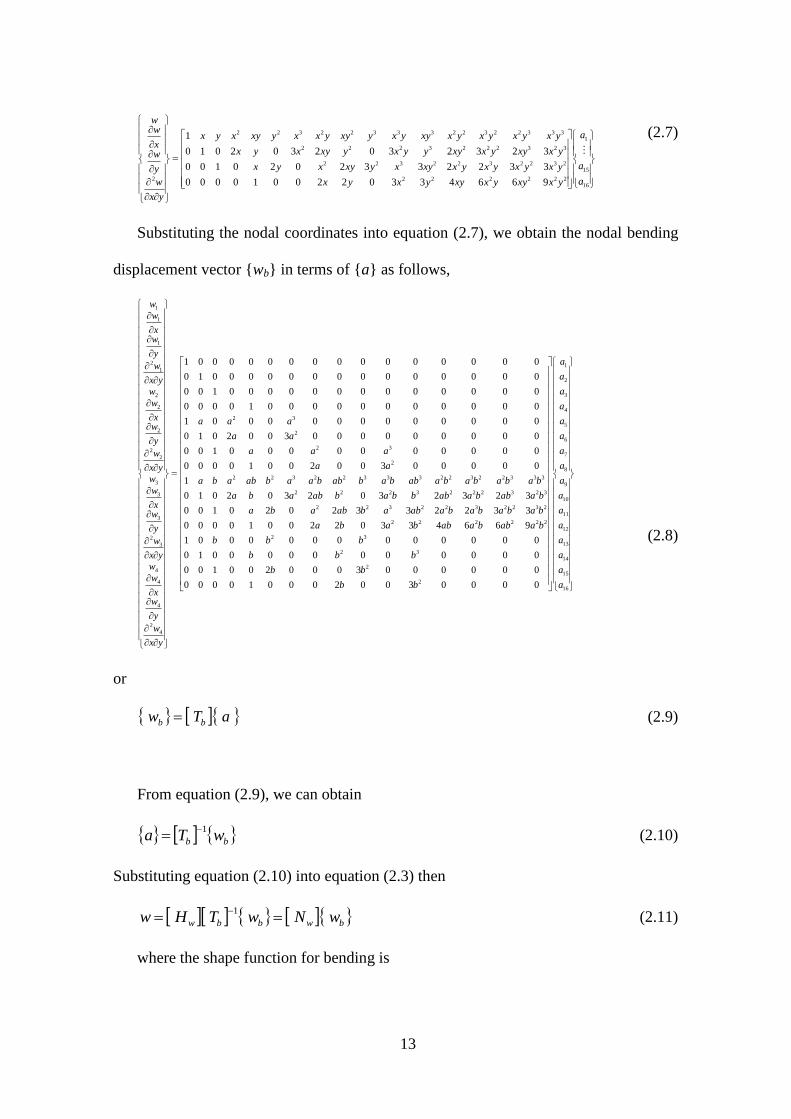
The displacement vector at each node for FE model is
T
vuyx
w
y
w
x
ww
2
(2.1)
The above displacement vector includes the membrane inplane displacement vector
Tvu and transverse displacement vector
T
yx
w
y
w
x
ww
2
.
The 16-term polynomial for the transverse displacement function is assumed in the
form
33
16
32
15
23
14
22
13
3
12
3
11
3
10
2
9
2
8
3
7
2
65
2
4321),(
yxayxayxayxaxyayxa
yaxyayxaxayaxyaxayaxaayxw
(2.2)
or in matrix form
}{
xxyxyxyx1 3332232233322322
aH
ayxyxyxyxxyyxyxyyw
w
(2.3)

12
where Taaaaaaaaaaaaaaaaa 16151413121110987654321}{ is
the transverse displacement coefficient vector. In addition, the two 4-term polynomials
for the inplane displacement functions can be written as
xybybxbbyxu 4321),( (2.4)
xybybxbbyxv 8765),( (2.5)
or in matrix form
}{
00001
bH
bxyyxu
u
and
}{
10000
bH
bxyyxv
v
(2.6)
where Tbbbbbbbbb 87654321 is the inplane displacement coefficient
vector. The coordinates and connection order of a unit 4-node rectangular plate element
are shown in Figure 2.1.
Figure 2.1. Node Numbering Scheme
2.2. Displacement Function in terms of Nodal Displacement
The transverse displacement vector at a node of the panel can be expressed by
13
16
15
1
222222
2322322322
3232223222
3332232233322322
29664330220010000
3322332020100
3232302302010
1
a
a
a
yxxyyxxyyxyx
yxyxyxyxxyxyxyxyx
yxxyyxxyyyxyxyxyx
yxyxyxyxxyyxyxyyxxyxyxyx
yx
w
y
wx
ww
(2.7)
Substituting the nodal coordinates into equation (2.7), we obtain the nodal bending
displacement vector {wb} in terms of {a} as follows,
16
15
14
13
12
11
10
9
8
7
6
5
4
3
2
1
2
2
32
32
222222
2322322322
3232223222
3332232233322322
2
32
2
32
4
2
4
4
4
3
2
3
3
3
2
2
2
2
2
1
2
1
1
1
0000300200010000
0000003000200100
0000000000010
0000000000001
9664330220010000
3322332020100
3232302302010
1
0000030020010000
0000000000100
0000000003002010
0000000000001
0000000000010000
0000000000000100
0000000000000010
0000000000000001
a
a
a
a
a
a
a
a
a
a
a
a
a
a
a
a
bb
bb
bbb
bbb
baabbaabbaba
babababaababababa
baabbaabbbabababa
babababaabbababbaabababa
aa
aaa
aa
aaa
yx
w
y
wx
w
w
yx
w
y
wx
w
w
yx
w
y
wx
w
w
yx
w
y
wx
w
w
(2.8)
or
aTw bb (2.9)
From equation (2.9), we can obtain
bb wTa1
(2.10)
Substituting equation (2.10) into equation (2.3) then
bwbbw wNwTHw 1
(2.11)
where the shape function for bending is
14
1 bww THN (2.12)
Similarly, the inplane displacement {u, v} can be expressed by
bxyyx
xyyx
v
u
10000
00001 (2.13)
Substituting the nodal coordinates into the equation (2.13), we can obtain the
inplane nodal displacement {wm} of the panel
8
7
6
5
4
3
2
1
4
4
3
3
2
2
1
1
0010000
0000001
10000
00001
0010000
0000001
00010000
00000001
b
b
b
b
b
b
b
b
b
b
abba
abba
a
a
v
u
v
u
v
u
v
u
(2.14)
or
bTw mm (2.15)
From (2.15),
mm wTb1
(2.16)
Substituting equation (2.16) into equation (2.6) gives
mummu wNwTHu 1
(2.17)
mvmmv wNwTHv 1
(2.18)
where the inplane shape functions are
1 muu THN (2.19)
1 mvv THN (2.20)

15
2.3. Nonlinear Strain Displacement Relation
The von Karman large deflection strain-displacement relation for the deflections u,
v, and w can be written as follows
yx
w
y
wx
w
z
y
w
x
w
y
w
x
w
x
v
y
u
y
vx
u
xy
y
x
2
2
2
2
2
2
2
2
2
1
2
1
(2.21)
or
zm (2.22)
where
m = membrane inplane linear strain vector,
= membrane inplane nonlinear strain vector,
z = bending strain vector.
The inplane linear strain can be written in terms of the nodal displacements as
follows
mmmmmm
vu
v
u
m wBwTCbCb
x
H
y
H
y
Hx
H
x
v
y
u
y
vx
u
1
(2.23)
where

16
yx
x
y
x
H
y
H
y
Hx
H
C
vu
v
u
m
010100
1000000
0000010
(2.24)
and
1 mmm TCB (2.25)
The inplane nonlinear strain can be written as follows
bbb
w
w
wBwTCaC
a
y
Hx
H
G
y
wx
w
x
w
y
w
y
wx
w
2
1][
2
1}{
2
1
}{2
1
2
10
0
2
1
1
(2.26)
where the slope matrix and slope vector are
x
w
y
w
y
wx
w
0
0
(2.27)
y
wx
w
G (2.28)
and

17
2322322322
3232223222
3322332020100
3232302302010
yxyxyxyxxyxyxyxyx
yxxyyxxyyyxyxyxyx
y
Hx
H
Cw
w
(2.29)
1 bTCB (2.30)
Combining equations (2.23) and (2.26), the inplane strain can be written as follows
bmmm ww BB2
1 (2.31)
The strain due to bending can be written in terms of curvatures as follows
}{}{}{
2
1
2
2
2
2
2
bbbbbb wBwTCaC
yx
w
y
wx
w
(2.32)
where
222222
3232
3322
2
2
2
2
2
1812128660440020000
6622606200200000
6262060026002000
2
yxxyyxxyyxyx
yxyxxxxyyx
xyyxyyxyyx
yx
w
y
wx
w
Cb
(2.33)
and
1 bbb TCB (2.34)
Thus, the nonlinear strain-nodal displacement relation can be written as
bbbmm
m
wzww
z
BBB
2
1
}{
(2.35)
18
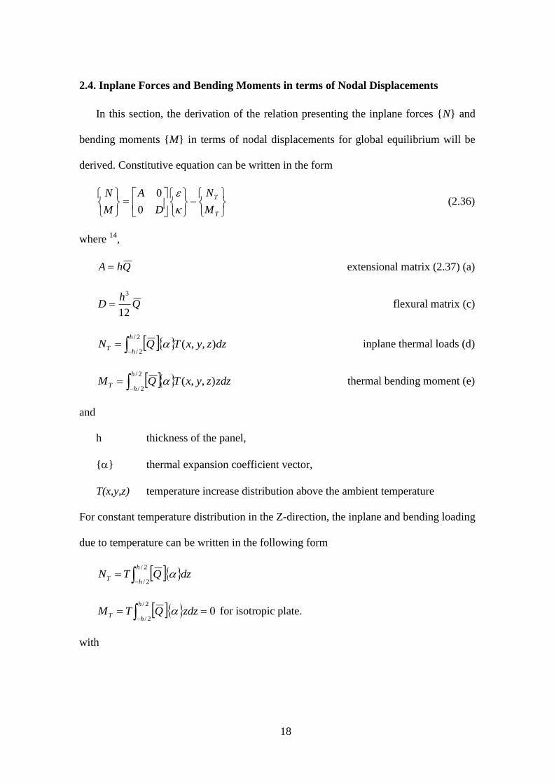
2.4. Inplane Forces and Bending Moments in terms of Nodal Displacements
In this section, the derivation of the relation presenting the inplane forces {N} and
bending moments {M} in terms of nodal displacements for global equilibrium will be
derived. Constitutive equation can be written in the form
T
T
M
N
D
A
M
N
0
0 (2.36)
where 14
,
QhA extensional matrix (2.37) (a)
Qh
D12
3
flexural matrix (c)
2/
2/),,(
h
hT dzzyxTQN inplane thermal loads (d)
2/
2/),,(
h
hT zdzzyxTQM thermal bending moment (e)
and
h thickness of the panel,
{} thermal expansion coefficient vector,
T(x,y,z) temperature increase distribution above the ambient temperature
For constant temperature distribution in the Z-direction, the inplane and bending loading
due to temperature can be written in the following form
2/
2/
h
hT dzQTN
02/
2/
h
hT zdzQTM for isotropic plate.
with

19
2
100
01
01
1][
2
EQ (2.38)
Expanding equation (2.36) gives
Tm
Tbmm
Tm
NNN
NwAwA
NAN
BB2
1
][
(2.39)
bb wDDM B][}]{[ (2.40)
2.5. Deriving the Element Matrices Using Principal of Virtual Work
Principal of virtual work states that
0int extWWW (2.41)
Virtual work done by internal stresses can be written as
V A
TT
ijij dAMNdVW }{}{int (2.42)
where
TTT
b
T
m
T
m
TT
m
T
ww
BB
(2.43)
and
T
b
T
b
Tw B (2.44)
Note that
GG
2
1

20
Substituting equations (2.39), (2.40), (2.43), and (2.44) into equation (2.42), the
virtual work done by internal stresses can be expressed as follows
dA
wDw
NwAwA
ww
WA
bb
T
b
T
b
Tbmm
TTT
b
T
m
T
m
BB
BB
BB
][
2
1
*
int
(2.45)
The terms of the expansion of equation (2.45) are listed as follows
mm
T
m
T
m wAw BB (2.46) (a)
b
T
m
T
m wAw BB2
1 (b)
T
T
m
T
m Nw B (c)
mm
TTT
b wAw BB (d)
b
TTT
b wAw BB2
1 (e)
T
TTT
b Nw B (f)
bb
T
b
T
b wDw BB ][ (g)
Terms (a) and (g) of equation (2.46) can be written in the matrix form as
m
b
m
b
mbw
w
k
kww
0
0 (2.47)
Where the linear stiffness matrices are
dADkA
b
T
bb BB ][][ (2.48)
dAAkA
m
T
mm BB][ (2.49)
21
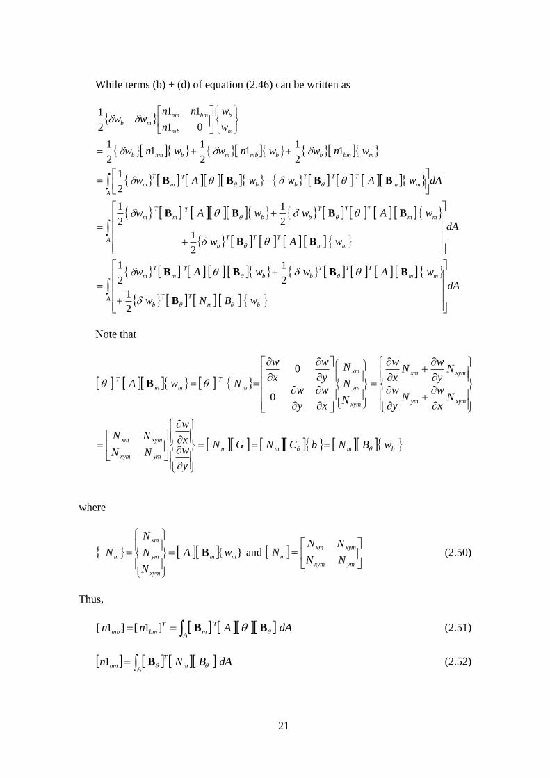
While terms (b) + (d) of equation (2.46) can be written as
Abm
TT
b
mm
TTT
bb
T
m
T
m
Amm
TTT
b
mm
TTT
bb
T
m
T
m
A
mm
TTT
bb
T
m
T
m
mbmbbmbmbnmb
m
b
mb
bmnm
mb
dA
wBNw
wAwwAw
dA
wAw
wAwwAw
dAwAwwAw
wnwwnwwnw
w
w
n
nnww
B
BBBB
BB
BBBB
BBBB
2
1
2
1
2
1
2
1
2
1
2
1
2
1
12
11
2
11
2
1
01
11
2
1
Note that
bmmm
ymxym
xymxm
xymym
xymxm
xym
ym
xm
m
T
mm
T
wBNbCNGN
y
wx
w
NN
NN
Nx
wN
y
w
Ny
wN
x
w
N
N
N
x
w
y
w
y
w
x
w
NwA
0
0
B
where
}{ mm
xym
ym
xm
m wA
N
N
N
N B
and
ymxym
xymxm
m NN
NNN (2.50)
Thus,
dAAnnA
T
m
T
bmmb BB]1[]1[ (2.51)
dABNnA
m
T
nm B1 (2.52)

22
The first order nonlinear stiffness matrices, nmmb nn 1&1 , are linearly dependent on
the node DOF {wm}([Nm]) and {wb}([]).
The second order nonlinear stiffness can be derived from term (e):
b
TTT
bb
T
b wAwwnw BB2
12
3
1
Thus,
dAAnA
TT
BB2
3]2[ (2.53)
Also
bT
TT
bT
TT
bT
TT
b
TyTxy
TxyTxTT
b
TxyTy
TxyTxTT
b
Txy
Ty
Tx
TT
bT
TTT
b
wBNwbCNwGNw
y
wx
w
NN
NNw
Nx
wN
y
w
Ny
wN
x
w
w
N
N
N
x
w
y
w
y
w
x
w
wNw
BBB
BB
BB
0
0
Thus,
dABNkA
T
T
TN B][ (2.54)
where
TyTxy
TxyTx
T NN
NNN (2.55)
Term (f) of equation (2.46) can be written in matrix form as follows
dANpA
T
T
mTm B (2.56)

23
2.5.1. Virtual work done by external forces
For the static problem, we may write:
A
Surfaceiiext
dAyxpw
dSuTW
),(
(2.57)
where T is the surface traction per unit area and p(x,y,t) is the external load vector. The
right hand side of equation (2.57) can be rewritten as b
T
b pw where
dAyxpNpA
T
wb ),( (2.58)
Finally, we may write
m
b
mb
bmnm
TN
m
b
W
W
N
N
NN
K
K
K
00
02
3
1
01
11
2
1
00
0
0
0
Tm
b
P
P 0
0 (2.59)
Equation (2.59) presents the static nonlinear deflection of a panel with thermal
loading, which can be written in the form
TTN PPWNNKK
2
3
11
2
1 (2.60)
Where
K is the linear stiffness matrix,
TNK is the thermal geometric stiffness matrix,
1N is the first order nonlinear stiffness matrix,
2N is the second order nonlinear stiffness matrix,

24
P is the external load vector,
TP is the thermal load vector,

25
3. Solution Procedures and Results of Panel Subjected to
Thermal Loading
The solution of the thermal loading problem of the panel involves the solution of the
thermal-buckling problem and the post-buckling deflection. In this chapter, the solution
procedure for predicting the behavior of panel will be presented.
For the case of constant temperature distribution, the linear part of equation 2.60 can
be written as follows
0 WKTK TN (3.1)
Which is an Eigenvalue problem in the critical temperature crT .
Equation (2.60) that describes the nonlinear relation between the deflections and the
applied loads can be also utilized for the solution of the post-buckling deflection. Recall
TTN PWNNKK
2
3
11
2
1 (2.60)
Introducing the error function W as follows
023
11
2
1
TTN PWNNKKW (3.2)
which can be written using truncated Taylor expansion as follows
WdW
WdWWW
(3.3)
26
where
tan21 KNNKK
dW
WdTN
(3.4)
Thus, the iterative procedures for the determination of the post-buckling displacement
can be expressed as follows
TiiiTNi PWNNKKW
2
3
11
2
1 (3.5)
iiiWWK 1tan (3.6)
ii WKWi
1
tan1 (3.7)
11 iii WWW (3.8)
Convergence occur in the above procedure, when the maximum value of the 1iW
becomes less than a given tolerance tol ; i.e. toliW 1max .
Figure 3.1 presents the variation of the maximum transverse displacement of the
panel when heated beyond the buckling temperature. Notice that the rate of increase of
the buckling deformation is very high just after buckling, then it decreases as the
temperature increases indicating the increase in stiffness due to the increasing influence
of the nonlinear terms.

27
0
0.5
1
1.5
2
2.5
6 11 16 21 26
Temperature Increase (C)
Wm
ax
/Th
ick
ne
ss
Figure 3.1. Variation of maximum deflection of the plate with temperature increase.

28
4. Derivation of the Finite Element Model for Panel-flutter
Problem
In this section, the formulation presented in section 2 will be extended to include the
dynamic (time dependent) terms. The aerodynamic formulation will be derived using
first order quasi-steady piston theory which gives quite accurate aerodynamic model at
high speed regimes.
4.1. Deriving the Element Matrices Using Principal of Virtual Works
Extending the principle of virtual work to include the inertial terms, we may write,
A
Viiext
dAt
vhv
t
uhutyxp
t
whw
dVuBW
2
2
2
2
2
2
),,(
(4.1)
where B is the body (inertial) forces per unit volume, T is the surface traction per unit
area, is the mass density per unit thickness, and h is the panel thickness.
The first term of (4.1) can be used to derive the bending mass matrix from
bb
T
b wmw , such that the bending mass matrix can be obtained by
dANNhmA
w
T
wb ][ (4.2)
Similarly, the inplane mass matrix can be obtained by
dANNNNhmA
v
T
vu
T
um ][ (4.3)
The equation of motions of the system can be written as
29
m
b
mb
bmnmTN
m
b
m
b
m
b
W
WN
N
NNK
K
K
W
W
M
M
00
02
3
1
01
11
2
1
00
0
0
0
0
0
TmP
0 (4.4)
4.2. 1st-Order Piston Theory
The fist order quasi-steady piston theory for supersonic flow, states that
x
w
a
D
t
w
a
Dg
x
w
t
w
vM
MqP a
a 3
110
4
110
0
1
1
22
(4.5)
where
Pa is the aerodynamic loading,
v the velocity of air-flow,
M Mach number,
q dynamic pressure =av2/2,
a air mass density,
12 M
,
ga non-dimensional aerodynamic damping
3
0
2 2
h
Mva
non-dimensional aerodynamic pressure 110
32
D
qa
o
2
1
4
110
ha
D
D110 is the first entry of the laminate bending D(1,1) when all the fibers of the
composite layers are aligned in the airflow x-direction.
a is the panel length

30
The virtual work of the quasi-steady 1st-order piston theory aerodynamic loading is
ba
T
bb
aT
b
b
w
A
T
w
T
bbw
a
A
T
w
T
b
A A
a
aext
waa
wwgg
w
dAwx
N
a
DNwdAwN
a
DgNw
dAx
w
a
D
t
w
a
DgwdAwPW
3
0
3
110
4
110
0
3
110
4
110
0
.
][
(4.6)
wheres the aerodynamic damping matrix [g] is defined by,
bbA
w
T
w MMha
DdAN
a
DNg 2
04
110
4
110
(4.7)
and the aerodynamic influence matrix [aa] is defined by,
dAx
NDNa w
A
T
wa
110
(4.8)
Finally, we get the equation of motion in the form
)(
23
11
2
13
0
tPP
WAa
NNKKWGg
WM
T
aTNa
(4.9)
where
0
)()(
00
0
00
0
0
0
tPtP
AA
GG
M
MM
b
a
a
m
b

31
5. Solution Procedure and Results of the Combined
Aerodynamic-Thermal Loading Problem
In this section, the procedure of determining the critical non-dimensional dynamic
pressure and the combined aerodynamic-thermal loading on the panel will be presented.
The mass terms, as well as the time dependent terms, will be introduced to the equation
of motion. The aerodynamic stiffness and damping terms are introduced by the quasi-
steady piston theory.
5.1. The Flutter Boundary
Recall from the previous chapter
)(
23
11
2
13
0
tPP
WAa
NNKKWGg
WM
T
aTNa
(4.9)
Which can be reduced for the solution of the linear (pre-buckling and pre-flutter)
problem to the following equation
)(12
13
0
tPPWNAa
KKWGg
WM TaTNa
(5.1)
Separating equations (5.1) into lateral and transverse directions, we obtain the following
two equations
)(12
13
0
tPPWNAa
KK
WGg
WM
bTbbnmaTNb
ba
bb
(5.2)

32
and
Tmmmmm PWKWM (5.3)
It can be assumed that the inplane mass term mM is negligible 12
. Thus, equation (5.2)
can be written in the form
Tmmm PKW
1 (5.4)
Note that the terms related to N2 and N1mb are dropped as they depend on Wb which is
essentially zero before buckling or flutter, while N1nm terms are kept as they depend in
Wm which might have non-zero values depending on the boundary conditions.
Substituting equation (5.4) into equation (5.2), we get
)(
12
1
1
3
0
tPPPK
WNAa
KK
WGg
WM
bTbTmm
bnmaTNb
b
a
bb
(5.5)
Solving the homogeneous form of equation (5.5) reduces to
012
13
0
bnmaTNbb
abb WNA
aKKWG
gWM
(5.6)
Now, assuming the deflection function of the transverse displacement bW to be in
the form of
t
bb ecW (5.7)
where i is the complex panel motion parameter ( is the damping ratio and
is the frequency), c is the amplitude of vibration, and b is the mode shape.

33
Substituting equation (5.7) into equation (5.6) we get,
0 t
bb eKMc (5.8)
where bob MM 2 , is the non-dimensional eigenvalue; given by
o
a
o
g
2
2
(5.9)
and
nmaTNb NAa
KKK 12
13
(5.10)
From equation (5.8) we can write the generalized eigenvalue problem
0 bb KM (5.11)
where is the eigenvalue, and b is the mode shape, with the charactaristic equation
written as,
0 KMb (5.12)
Given that the values of are real for all values of below the critical value, the
iterative solution can be utilized to determine the critical non-dimensional dynamic
pressure cr for temperatures less than the critical buckling temperature.
34
5.2. The Combined Loading Problem
In this section, the procedures used to determine the buckling temperature under the
influence of aerodynamic loading as well as the flutter boundary variation with elevated
temperatures is presented. Recall the stiffness term from equation (5.10)
anmTNb Aa
NKKK3
12
1 (5.10)
This equation contains the combined effect of thermal and aerodynamic loading. In
other words, the aerodynamic stiffness term ( aAa3
) can be added to the procedure of
section 3.2 to obtain the critical buckling temperature to investigate the effect of
changing the dynamic pressure on the buckling temperature.
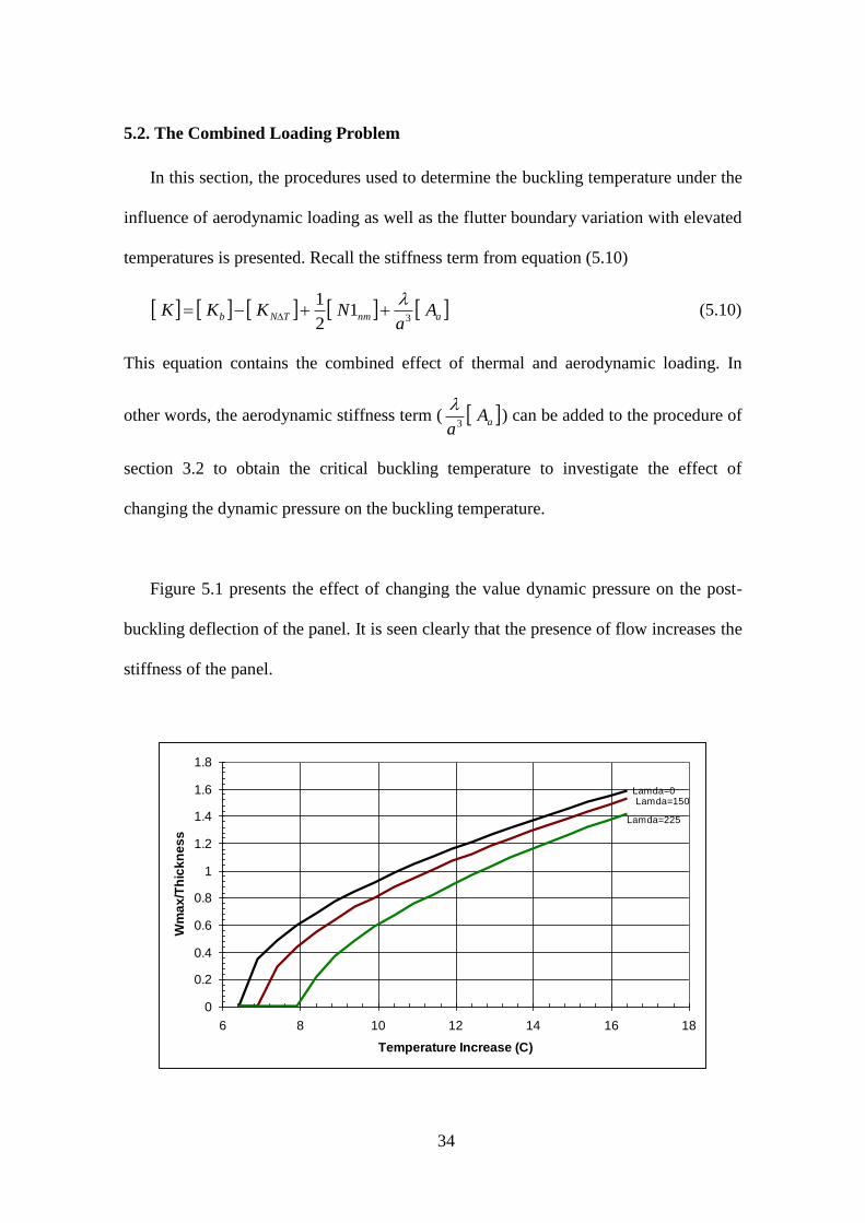
Figure 5.1 presents the effect of changing the value dynamic pressure on the post-
buckling deflection of the panel. It is seen clearly that the presence of flow increases the
stiffness of the panel.
0
0.2
0.4
0.6
0.8
1
1.2
1.4
1.6
1.8
6 8 10 12 14 16 18
Temperature Increase (C)
Wm
ax
/Th
ick
ne
ss
Lamda=0Lamda=150
Lamda=225

35
Figure 5.1. Variation of the maximum post-buckling deflection for different values of the dynamic
pressure.
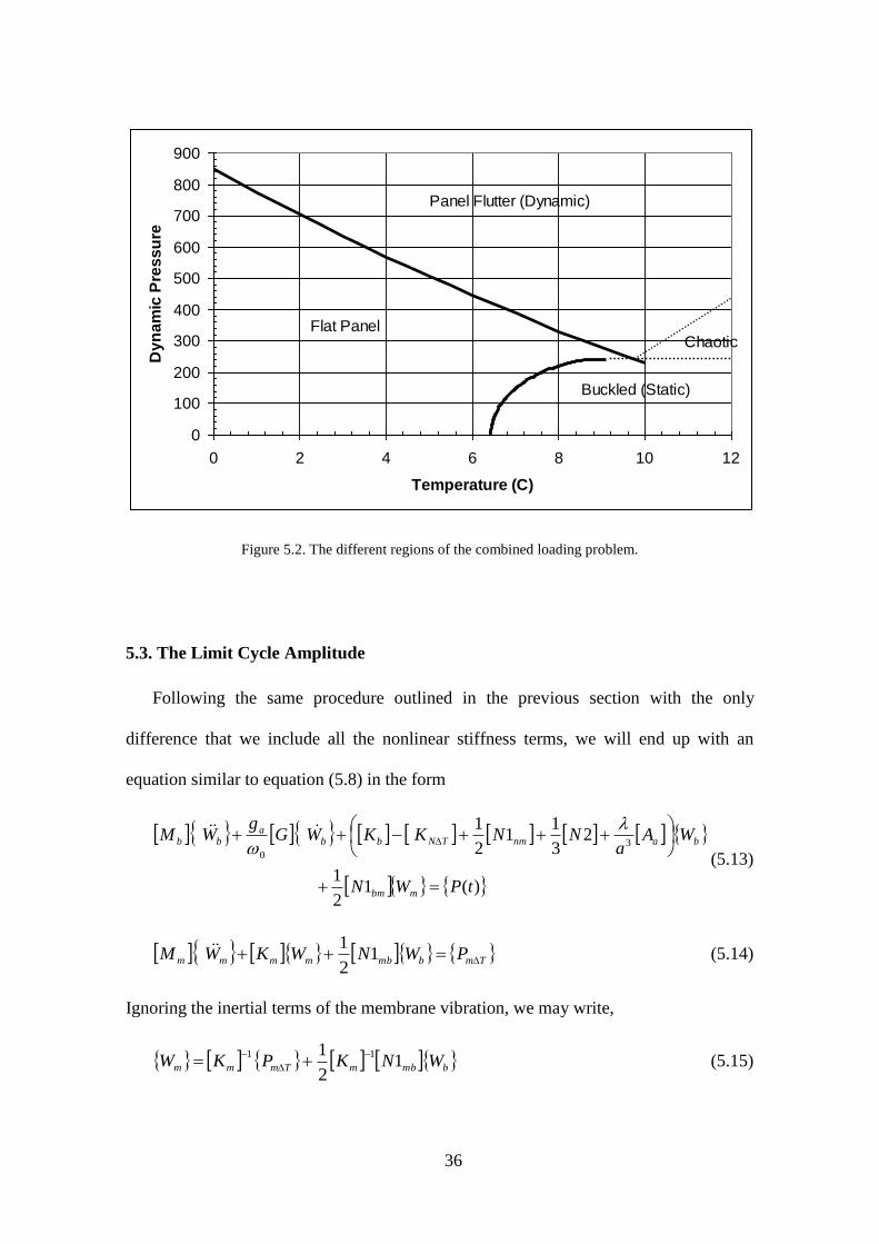
Figure 5.2 presents a combined chart of the different regions of the combined
loading problem. The “Flat” region indicates the different combinations of dynamic
pressure and temperature increase through which the panel will neither undergo flutter
norbuckling.The“Buckled”region indicates the combination of dynamic pressure and
temperature increase under which the panel undergoes static deflection due to buckling.
Note that the curve indicating the change of the buckling temperature with dynamic
pressure reaches an asymptotic valueatdynamicpressureof242.The“PanelFlutter”
region indicates the combination of temperature and dynamic pressure under which the
panel undergoes pure panel flutter; in other words, the panel becomes stiff enough, due
to the aerodynamic pressure, thatisdoesnotsufferanybuckling.Finally,the“Chaotic”
region indicates the combination of temperature increase and dynamic pressure under
which the plate undergoes limit cycle flutter about a static deflection position due to
thermal buckling. This final region is not going to be investigated in this project.
36
0
100
200
300
400
500
600
700
800
900
0 2 4 6 8 10 12
Temperature (C)
Dy
na
mic
Pre
ss
ure
Flat Panel
Buckled (Static)
Panel Flutter (Dynamic)
Chaotic
Figure 5.2. The different regions of the combined loading problem.
5.3. The Limit Cycle Amplitude
Following the same procedure outlined in the previous section with the only
difference that we include all the nonlinear stiffness terms, we will end up with an
equation similar to equation (5.8) in the form
)(12
1
23
11
2
13
0
tPWN
WAa
NNKKWGg
WM
mbm
banmTNbba
bb
(5.13)
Tmbmbmmmm PWNWKWM 12
1 (5.14)
Ignoring the inertial terms of the membrane vibration, we may write,
bmbmTmmm WNKPKW 12
1 11
(5.15)

37
Substituting into the bending displacement equation we get,
)(12
111
4
1
23
11
2
1
11
3
0
tPPKNWNKN
WAa
NNKKWGg
WM
Tmmbmbmbmbm
banmTNbba
bb
(5.16)
It can be shown that,
bmbmbmbnm WNKNWN 112
11
1
Which can be used to write the bending equation in its final form to be,
)(12
1
23
111
2
1
1
1
3
0
tPPKN
W
NNKN
Aa
KK
WGg
WM
Tmmbm
b
mbmbm
aTNb
ba
bb
(5.17)
Procedure similar to those described earlier can be used to write down the equation
of motion in the form,
0 t
bb eKMc (5.18)
Where,
23
111
2
1 1
3NNKNA
aKKK mbmbmaTNb
Since the nonlinear stiffness terms of the above equation depend on the amplitude of the
vibration, an iterative scheme should be used. The following algorithm outlines the
steps used in the iterative procedure.
1- Normalize the Eigenvector {}, obtained at the flutter point, using the
maximum displacement.

38
2- Select a value for the amplitude c
3- Evaluate the linear and nonlinear stiffness terms.
4- Change the value of the nondimensional aerodynamic pressure .
5- Solve the eigenvalue problem for .
6- If coelacence occurs proceed, else goto step 4
7- Check the differences between the obtained eigenvector and the initial, if small,
proceed, else normaize the eigenvector as described in step 1 and go to step 3.
8- The obtained dynamic pressure corresponds to the initially given amplitude
9- Go to step 2
It have to be noted that the above mentioned procedure is valid for the case when
panel flutter occurs while the plate is not buckled or when the dynamic pressure is high
enough that the buckled plate flat again; which does not cover the region of chaotic
vibration.
Figure 5.3 Presents and extended version of Figure 5.2. In this figure, we can notice
the linear variaiotn of the dynamic pressure associated with different limit cycle
amplitudes in the panel flutter region.
Figure 5.4 presents a full map of the variation of both the limit cycle amplitude as
well as the post-buckling deflection with the dynamic pressure for different values of
the temperature increase. Note the distinction between the static and the dynamic
regions.

39
0
200
400
600
800
1000
1200
0 2 4 6 8 10
Temperature (C)
Dy
na
mic
Pre
ss
ure
Flutter Limit (C=0)
C=1C=0.8C=0.5
Buckling Limit (Wmax=0)
Figure 5.3. Variation of the dynamic pressure associated with different limit cycle amplitudes with
temperature.
0
0.2
0.4
0.6
0.8
1
1.2
0 200 400 600 800 1000 1200
Non-Dimensional Dynamic Pressure
Wm
ax
/Th
ick
ne
ss
DT=0DT=3.4DT=6.4=TcrDT=9.4
DT=6.9
Buckling Flutter
DT=9.4
DT=10.4
DT=7.4
DT=8.4
Figure 5.4. Variation of the limit cycle amplitude with dynamic pressure as well as the variation of the
post-buckling amplitude with dynamic pressure for different values of the temperature increase.

40
6. Concluding Remarks
This project report presents an extension of an earlier study that involved the post
buckling deflection and the investigation of the effect of temperature on the flutter
boundary of composite plate embedded with shape memory alloy fibers29
. The
extension presented here is the investigation of the limit cycle vibration of the panel
which is an essentially nonlinear dynamics problem.
The other aspect that is not presented in this study is the investigation of the chaotic
vibration region. This region requires the separation of the solution into two distinct
values, namely the static deflection, which is due to the thermal loading, and the
dynamic deflection, which is due to the flutter. The expansion involves extra nonlinear
terms but is essentially straight forward from the point of stand of the current study30
.

41
References
1 Mei,C.,“AFiniteElementApproachforNon-linear panel-flutter,”AIAA Journal,
Vol. 15, No. 8, 1977, pp. 1107-1110.
2 Zhou,R.C.,Xue,D.Y., andMei,C., “OnAnalysis ofNonlinearPanel-flutter at
Supersonic Speeds,” Proceedings of the First Industry/Academy Symposium On
Research For Future Supersonic And Hypersonic Vehicles, Vol. 1, Greensboro,
North Carolina, 1994, pp. 343-348.
3 Xue,D.Y., andMei, C., “Finite ElementNon-linear Panel-flutter with Arbitrary
TemperatureinSupersonicFlow,”AIAA Journal, Vol. 31, No. 1, 1993, pp. 154-162.
4 Frampton, K. D., Clark, R. L., and Dowell, E. H., “State-Space Modeling For
AeroelasticPanelsWithLinearizedPotentialFlowAerodynamicLoading,”Journal
Of Aircraft, Vol. 33, No. 4, 1996, pp. 816-822.
5 Dowell,E.H.,“PanelFlutter:AReviewofTheAeroelasticStabilityofPlates and
Shells,”AIAA Journal, Vol. 8, No. 3, 1970, pp. 385-399.
6 Bismarck-Nasr, M. N., “Finite Element analysis of Aeroelasticity of Plates and
Shells,”Applied Mechanics Review, Vol. 45, No. 12, 1992, pp. 461-482.
7 Bismarck-Nasr, M. N., “Finite Elements in Aeroelasticity of Plates and Shells,”
Applied Mechanics Review, Vol. 49, No. 10, 1996, pp. S17-S24.

42
8 Mei, C., Abdel-Motagaly,K.,andChen,R.,“ReviewofNonlinearPanelFlutterat
Supersonic andHypersonicSpeeds,”Applied Mechanics Review, Vol. 52, No. 10,
1999, pp. 321-332.
9 Sarma, B. S., and Varadan, T. K. “Non-linear Panel-flutter by Finite Element
Method,”AIAA Journal, Vol. 26, No. 5, 1988, pp. 566-574.
10 Yang,T.Y., and Sung, S.H. “FiniteElement Panel-flutter in Three-Dimensional
Supersonic Unsteady Potential Flow,” AIAA Journal, Vol. 15, No. 12, 1977, pp.
1677-1683.
11 Ashley,H.,andZartarian,G.,“PistonTheory– A New Aerodynamic Tool for the
Aeroelastician,”Journal of Aeronautical Sciences, Vol. 23, No. 12, 1956, pp. 1109-
1118.
12 Dixon, I. R., and Mei, C., “Finite Element Analysis of Large-Amplitude Panel-
flutterofThinLaminates,”AIAA Journal, Vol. 31, No. 4, 1993, pp. 701-707.
13 Abdel-Motagaly,K.,Chen,R.,andMei,C.“NonlinearFlutterofCompositePanels
Under Yawed Supersonic Flow Using Finite Elements,”AIAA Journal, Vol. 37, No
9, 1999, pp. 1025-1032.
14 Zhong,Z.“ReductionofThermalDeflectionAndRandomResponseOfComposite
Structures WithEmbeddedShapememoryAlloyAtElevatedTemperature”,PhD
Dissertation, 1998, Old Dominion University, Aerospace Department, Norfolk,
Virginia.

43
15 Frampton,KennethD.,Clark,RobertL., andDowell,EarlH. “ActiveControlOf
Panel-flutterWithLinearizedPotentialFlowAerodynamics”,AIAAPaper95-1079-
CP, February 1995.
16 Gray, C. E., Mei, C., and Shore, C. P.,“FiniteElementMethodforLarge-Amplitude
Two-Dimensional Panel-flutteratHypersonicSpeeds,”AIAA Journal, Vol. 29, No.
2, 1991, pp. 290-298.
17 Benamar,R,Bennouna,M.M.K.,andWhiteR.G.“Theeffectof largevibration
amplitudes on the mode shapes and natural frequencies of thin elastic structures
PART II: Fully Clamped Rectangular Isotropic Plates”, Journal of Sound and
Vibration, Vol. 164, No. 2, 1993, pp. 295-316.
18 Benamar,R,Bennouna,M.M.K.,andWhiteR.G.“Theeffectof largevibration
amplitudes on the mode shapes and natural frequencies of thin elastic structures
PARTIII: Fully Clamped Rectangular Isotropic Plates – Measurements of The Mode
Shape Amplitude Dependence And The Spatial Distribution Of Harmonic
Distortion”,Journal of Sound and Vibration, Vol. 175, No. 3, 1994, pp. 377-395.
19 Liu, D. D., Yao, Z. X., Sarhaddi, D., and Chavez, F., “From Piston Theory to
Uniform Hypersonic-SupersonicLiftingSurfaceMethod,”Journal of Aircraft, Vol.
34, No. 3, 1997, pp. 304-312.
20 Lee, I., Lee, D.-M., and Oh, I.-K, “Supersonic Flutter Analysis of Stiffened
LaminatedPlatesSubject toThermalLoad,”Journal of Sound and Vibration, Vol.
224, No. 1, 1999, pp. 49-67.

44
21 Surace, G. and Udrescu, R., “Finite-Element Analysis of The Fluttering Panels
Excited byExternalForces,”Journal of Sound and Vibration, Vol. 224, No. 5, 1999,
pp. 917-935.
22 Bismarch-Nasr,M.N.andBones,A.,“DampingEffectsinNonlinearPanelFlutter,”
AIAA Journal, Vol. 38, No. 4, 2000, pp. 711-713.
23 Young, T. H. and Lee, C. W., “Dynamic Stability of Skew Plates Subjected to
Aerodynamic and Random In-PlaneForces,”Journal of Sound and Vibration, Vol.
250, No. 3, 2002, pp. 401-414.
24 Zhou, R.C., Lai, Z., Xue, D. Y., Huang, J. K., and Mei, C., “Suppression Of
Nonlinear Panel-flutter with PiezoelectricActuatorsUsingFiniteElementMethod”,
AIAA Journal, Vol. 33, No. 6, 1995, pp. 1098-1105.
25 Frampton,K.D.,Clark,R.L.,andDowell,E.H.,“ActiveControlOfPanel-flutter
WithPiezoelectricTransducers,”Journal Of Aircraft, Vol. 33, No. 4, 1996, pp. 768-
774.
26 Dongi, F., Dinkler, D., and Kroplin, B. “Active Panel-flutter Suppression Using
Self-SensingPiezoactuators,”AIAA Journal, Vol. 34, No. 6, 1996, pp. 1224-1230.
27 Scott, R. C., and Weisshaar, T. A., “Controlling Panel-flutter Using Adaptive
Materials,”AIAAPaper91-1067-CP, 1991.
28 Suzuki, S. and Degali, T., “Supersonic Panel-flutter Suppression Using Shape
Memory Alloys,” International Journal of Intelligent Mechanics: Design and
Production, Vol. 3, No. 1, 1998, pp. 1-10.
45
29 Tawfik, M., Ro, J. J., and Mei, C., “Thermal post-buckling and aeroelastic
behaviourofshapememoryalloyreinforcedplates,”SmartMaterialsandStructures,
Vol 11, No. 2, 2002, pp. 297-307.
30 Xue,D.Y.,“FiniteElementFrequencyDomainSolutionofNonlinearPanel-flutter
WithTemperatureEffectsAndFatigueLifeAnalysis”,PhDDissertation,1991,Old
Dominion University, Mechanical Engineering Department, Norfolk, Virginia.