SANDIA REPORTSAND97–8224 • UC–406Unlimited ReleasePrinted January 1997

Finite Element Analyses of ToolStresses in Metal Cutting Processes

Bruce L. Kistler

Prepared bySandia National LaboratoriesAlbuquerque, New Mexico 87185 and Livermore, California 94551for the United States Department of Energyunder Contract DE-AC04-94AL85000

Approved for public release; distribution is unlimited.

2

This Page is Intentionally Blank

3

DistributionCategory UC-406

SAND97-8224Unlimited Release

Printed January 1997

Finite Element Analyses of Tool Stressesin Metal Cutting Processes

Bruce L. KistlerStructural and Thermomechanical Modeling Department

Sandia National LaboratoriesLivermore, California 94550

Abstract

In this report, we analytically predict and examine stresses in tool tips used in high speedorthogonal machining operations. Specifically, one analysis was compared to an existingexperimental measurement of stresses in a sapphire tool tip cutting 1020 steel at slowspeeds. In addition, two analyses were done of a carbide tool tip in a machining processat higher cutting speeds, in order to compare to experimental results produced as part ofthis study. The metal being cut was simulated using a Sandia-developed damage-plasticity material model, which allowed the cutting to occur analytically without pre-specifying the line of cutting/failure. The latter two analyses incorporated temperatureeffects on the tool tip. Calculated tool forces and peak stresses matched experimentaldata to within about 20%. Stress contours generally agreed between analysis andexperiment. This work could be extended to investigate/predict failures in the tool tip,which would be of great interest to machining shops in understanding how to optimizecost/retooling time.

4

Acknowledgments

This study was funded under the Laboratory Directed Research and Development(LDRD) project “Impact & Thermal Shock Response of Metal Cutting Tools for HighStrength, High Speed Milling Operations” case # 3507240000, which was a two-yearproject closing at the end of Fiscal Year 1996.

Special thanks go to Anil Reddy, who as a co-op student performed most of the detail ofthe final Bagchi calculation, and whose excellent internal memorandum write-up wasused extensively in this report. Also, special recognition goes to Al McDonald, whoinitiated and managed this project for the first year.

5

Table of Contents

Introduction ......................................................................................................................... 8Bagchi’s Work................................................................................................................... 10Sandia Damage/Plasticity Model ...................................................................................... 11Conjugate Gradient Method.............................................................................................. 12Analysis of Bagchi Experiments ....................................................................................... 13Comparison of Analysis to Bagchi’s Experimental Data.................................................. 17Sandia Experiments and Results ....................................................................................... 20Analyses of Sandia Experiments....................................................................................... 21Comparison of Experimental and Numerical Results ....................................................... 27Implications of Results and Useful Future Work.............................................................. 34Conclusions/Summary ...................................................................................................... 35References ......................................................................................................................... 36Appendix A: Internal Memorandum of Finite Element Calculations of Bagchi [2] Experiment ........................................................................... 37Appendix B: Internal Memorandum of Finite Element Analysis Parameter Study

Based on Experiments by Bagchi [2] ......................................................... 38

List of Figures

Figure 1: In Orthogonal Cutting, Tool Edge is Normal to Direction of Motion................ 9Figure 2: The Setup Used in Bagchi’s Experiment [2] .................................................... 14Figure 3: Finite Element Mesh Used for Analysis of Bagchi Experiments ..................... 15Figure 4: Finite Element Mesh at Tool Tip for Bagchi Experiments............................... 15Figure 5: Comparison of Cutting Direction Stress (MPa) for Bagchi Experiment.......... 17Figure 6: Comparison of Thrust Direction Stress (MPa) for Bagchi Experiment............ 19Figure 7: Comparison of Shear Stress (MPa) for Bagchi Experiment ............................. 19Figure 8: Finite Element Mesh Used for Modeling Sandia Experiments ........................ 22Figure 9: Finite Element Mesh at the Tool Tip for Sandia Experiments ......................... 22Figure 10: Predicted Tool Temperature Contours

for 6061-T6 Aluminum Workpiece (F)........................................................... 23Figure 11: Predicted Tool Temperature Contours

for 304L Stainless Steel Workpiece (F) .......................................................... 24Figure 12: Thrust Direction Tool Strains for 6061-T6 Aluminum Workpiece................ 28Figure 13: Cutting Direction Tool Strains for 6061-T6 Aluminum Workpiece .............. 29Figure 14: Tool Shear Strains for 6061-T6 Aluminum Workpiece ................................. 30Figure 15: Thrust Direction Tool Strains for 304L Stainless Steel Workpiece ............... 31Figure 16: Cutting Direction Tool Strains for 304L Stainless Steel Workpiece.............. 32Figure 17: Tool Shear Strains for 304L Stainless Steel Workpiece................................. 34

List of Tables

6

Table 1: Properties used in the Sandia Damage/Plasticity Model for 1020 Steel............ 16Table 2: Material Properties Used in Analysis for Carbide Tool..................................... 24Table 3: Properties Used in the Sandia Damage/Plasticity Model

for 6061-T6 Aluminum and 304L Stainless Steel.............................................. 26Table 4: Measured Microstrain at Specific Locations for Sandia Experiments............... 27

7

This page is intentionally blank

8

Introduction

Machining is a common fabrication technique where material is shaved from a part usinga tool with a small, hard tip. Usually the material being cut is a metal, such as aluminumor steel, and the standard tool tip is commonly a carbide material. The carbide is oftencoated with a thin diamond coating to increase the life of the tool tip. In order to quicklyfabricate a part, a high cutting speed is desired. These higher speeds, however, lead to afaster degradation of the tool tip, which requires that the tool tip be replaced morefrequently. Over the history of machining, guidelines and conventions have arisen basedon empirical information of tradeoffs between cutting speed and tool replacement time.

A significant amount of experimental and analytical work has been done on the behaviorof the material being cut. The reason is that the final machined product must meet certaindesign specifications. On the other hand, very little attention has been paid analytically tounderstanding the behavior of the tool, specifically with regard to extending it’s lifetime.This lack of numerical investigation of tool response is surprising, given the possible costand time savings of extending the life of the tool, which allows either faster cuttingspeeds or a longer time between retooling.

The purpose of this study was to attempt to both experimentally measure and analyticallymodel the behavior of specific tool tips under controlled cutting conditions. Bysuccessfully modeling the behavior and response of the tool tip, we believed that wecould then make recommendations for extending tool life based on understanding of thetool failure mechanisms.

To reach that goal, we first examined the existing literature and found only one instancewhere tool responses, such as stress, had been experimentally measured. With thisexperimental data, a first finite element calculation was performed to determine therequired analytical parameters to effectively predict the tool tip response. The secondstep was to design and execute some carefully and specifically designed cuttingexperiments which would provide additional data from other cutting conditions than wereavailable in the literature. Finite element calculations were then performed to compareagainst this new data. Further refinements of the modeling process could then be made.The final step was to propose likely failure mechanisms and examine perturbations ingeometry and/or materials which would make those failures less likely to occur.

In examining failures of tool tips, several different mechanisms appear to be at work.Failure types include getting a built-up-edge, cratering, fracturing of the tip, etc. To someextent, these different types of failure may be associated with different types of cuttingenvironments. For instance, tip fracturing is more likely to occur in an interrupted cuttingscenario (such as lathing an object that has an axial groove which the tool would hit atevery rotation). In this case, shock waves are generated in the tool both as the tool entersand exits the groove, and these shock waves eventually fail the tool tip. Conversely, alonger continuous cut might lead to a built-up edge, which dulls the tool and therefore

9

requires more force for the cutting process. In addition, chips from the cut metal arecontinuously sticking/sliding over the tool tip, leading to variable local tip stresses whichact as a cyclic load. Finally, the process of cutting causes both the material being cut andthe local tool tip to heat up, which usually is associated with a decrease in materialstrength and other properties.

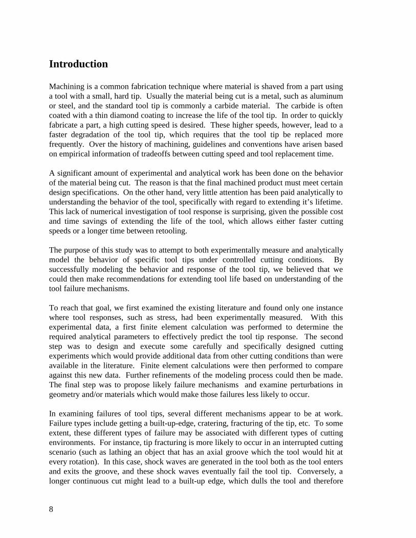
There are also different classifications of machining operations, each of which may havea different force or stress distribution. In orthogonal cutting, the tool edge is normal tothe direction of relative motion between the tool and the work material (Figure 1). Thelateral spread of the chip is ignored and the deformation process is assumed to be twodimensional. It can be easily achieved by machining the rim of a tube held in a lathe.Orthogonal cutting was the only cutting configuration examined in this study.

In this study, we specifically examined the thermal process, the interrupted cut shockwave scenario, a continuous cut which might lead to a relatively steady state stresscondition, and the tool tip stress changes that arise from different geometries associatedwith failure (such as the built-up edge and cratering). Different parts of this study wereundertaken by different personnel, and are written up separately [1]. This report will onlydiscuss the steady state cutting process. Although the original goal of this LDRD(Laboratory Directed Research and Development) project was to be able to understandand predict failure of the tool, this report only covers the finite element calculation ofsteady state stresses in the tool, and does not address failure mechanisms directly.

Figure 1: In Orthogonal Cutting, Tool Edge is Normal to Direction of Motion

The literature search found only one instance where stresses had been experimentallymeasured in a tool tip. In 1983, Bagchi [2] published a doctoral thesis documenting his

WorkMaterial

Flank Face

Tool

FinishedSurface

Initial WorkSurface

Chip

Rake Face

10

work, where he experimentally measured stresses in sapphire tools under slow speedorthogonal cutting conditions. This work became the starting point for our study.

Bagchi’s Work

Bagchi’s work [2] was divided into qualitative and quantitative experiments. In thequalitative experiments, he examined the chip-tool interaction both photographically andthrough post-test observation. In the quantitative experiments, the measurements whichBagchi made were the tool forces, tool stresses (measured as described below), andcontact length of the chip. For both sets of experiments, the materials being cut included360 brass, 1020 steel, and 12L14 steel. Bagchi also used 6061-T6 aluminum in thequalitative experiments. For the qualitative experiments, he used sapphire tool tips (forslow cutting speeds) and carbide tool tips (for commercial cutting speeds), while for thequantitative experiments he used only a sapphire tool tip.

Bagchi used a sapphire tool in his cutting experiments because sapphire is a birefringentmaterial. When load is applied to a birefringent material, ordered sets of lines, calledisochromatics and isoclinics, can be observed on the tool surface. The isochromatics andisoclinics are obtained using a plane polariscope. White light produces brightly coloredisochromatics and a diffused dark isoclinic. The different isoclinics are obtained for each15° interval rotation of the polarizer-analyzer combination. The isochromatics areassigned consecutive integer values while the isoclinics are assigned angles based on thepolarizer-analyzer orientation. The isochromatic integers are multiplied by the stressfringe constant (which Bagchi determines via Flamant's line loading technique [3]). Theresulting values are the differences in principal stresses along each isochromatic line.The isoclinic angles show the path of the principal stress angle (theta).

Given Bagchi's mapping of the isochromatics and isoclinics, isocline data were found atnodes on a superimposed mesh through interpolation. Bagchi uses the shear differencemethod to determine the stresses at each of these nodes. The method requires animposition of suitable boundary conditions and involves marching numerically from aninternal row within the tool to the rake face. In order to begin the difference marching,one needs to know the stresses at a particular point. Therefore, he assumed that the shearforce and the stress normal to the flank face of the tool were nearly zero at the nodefarthest from the cutting edge on the flank face. This started the forward differencecalculation for 1-direction stresses. Values for the 2-direction stresses were determinedusing the Mohr's Circle relationship with known shear stress, 1-direction stress, and thedifference between principal stresses. Once the stresses are determined in that row of themesh, stresses in the adjacent row were similarly determined using forward difference.The stresses in the following rows were calculated using a central difference technique.Bagchi included a mapping of isoclinics and isochromatics for the 1020 steel experimentbut plotted normal and shear stress for the rake face only. In order to more thoroughlycompare the analysis to experiment, we determined the stresses at all the nodes on theentire 1-2 plane of the tool. This required going through an interpolation of Bagchi's raw

11

isochromatic and isoclinic data and rewriting his shear difference program to evaluate thestress profile for a 3.39 millimeter square on the 1-2 plane. A 20 by 20 node mesh wasused for the shear difference technique.

Sandia Damage/Plasticity Model

Different techniques have been used in the past to analytically model the metal cuttingprocess. Attempts to model the process of chip formation have for the most part beenbased on a predetermined line of separation between the workpiece and chip (e.g.,Strenkowski and Carroll [4]; Komvopoulos and Erpenbeck [5]). Nodes on this line areseparated, and the line “unzipped”, when the tool tip is sufficiently close, or when acertain level of plastic strain is attained. Obviously, this approach makes assumptionsboth on the location and stress level of the “failure” which is the cutting of the metal, andis therefore undesirable in understanding the process. Sekhon and Chenot [6] andMarusich and Ortiz [7], by contrast, have used mesh adaptivity and remeshing to allowfor an arbitrary surface of separation. This approach is much more desirable because itmore accurately models the cutting process. However, it is a complicated and time-consuming task to numerically perform the remeshing and mesh adaptivity and is stilldependent on the material model to correctly describe the behavior of each elementmaking up the workpiece.

In this study, we employed an intermediate approach. We believe that a complexcoupling exists between the tool and workpiece that is a function of the forces,temperature, and history. However, the specific details of chip formation anddeformation of the workpiece may not have a direct or significant affect on the tool-workpiece forces or temperature, as long as the overall cutting process is “correct”. Ingeneral, the location of the cut will be in approximately the location and direction of thetool tip. Thus, we chose to use a finite element mesh which was oriented in thatdirection. Then, to accurately represent the damage and failure in the workpiece and chip,the Sandia Damage/Plasticity Model [8] was used. This model allows the calculation ofaccumulated damage in a finite element. Then, we used a capability of the ABAQUS [9]finite element code to turn finite elements “off” when a user-defined parameter level wasreached in each element. This eliminated elements which otherwise would have hadlarge distortions (causing convergence problems in the analysis) but which physically hadfailed or had lost their load carrying capability. Using this approach, we believe that wecan adequately represent the cutting/failure/chip formation mechanisms without requiringremeshing or mesh adapting.

The Sandia Damage/Plasticity material model [8] is a material model which accounts forthe deviatoric deformation resulting from the presence of dislocations and dilatationaldeformation and ensuing failure from the growth of voids. The kinematics of the modelare based upon the multiplicative decomposition of the deformation gradient into elastic,deviatoric plastic, and dilatational plastic parts. The constitutive model is formulatedwith respect to the natural configuration (stress free) defined by the plastic deformation.This results in a structure whose current configuration stress variables are convected with

12

the elastic spin. To model the deviatoric plastic flow, both a scalar and a tensor internalvariable are introduced to describe the effects of dislocations in cell walls and cellinteriors respectively. The evolution equations for these variables are motivated fromdislocation mechanics and are in a hardening minus recovery format. The use of internalstate variables and the proposed evolution equations, enables the prediction of strain ratehistory and temperature history effects. These effects can be quite large and cannot bemodeled by equation-of-state models which assume that stress is a unique function of thestrain, strain rate, and temperature and independent of the loading path. The temperaturedependence of the hardening and recovery parameters results in the prediction of thermalsoftening during adiabatic temperature rises, and an additional softening is possible dueto the anisotropy associated with the evolution of the tensor variable.

The effects of damage due to the growth of voids is included through the introduction of ascalar internal state variable. This variable tends to degrade the elastic moduli of thematerial as well as to concentrate the stress in the deviatoric flow rule, thereby increasingthe plastic flow and leading to another mechanism of softening. When the damagereaches a critical value, failure ensues. The Cocks-Ashby model of the growth of aspherical void in a rate dependent plastic material is used as the internal state variable todescribe the evolution of the damage [10]. This equation introduces only one newparameter since it is strongly dependent upon the deviatoric plasticity model.

Conjugate Gradient Method

In a typical machining operation, thin layers of material are cut off in a repetitive processuntil the desired total thickness has been cut. In order to accurately capture the behaviorof a single layer using finite elements, several elements through the thickness of a singlelayer are required. Furthermore, finite elements perform best when they are not distorted:that is, where each edge has the same length or at least within a factor of 3 (aspect ratio of3 to 1). Thus, a large number of small elements were required to model the workpiecebehavior accurately, in order to predict the correct load and distribution into the tool tip(which is the structure we were really interested in for this study). For this study, fiveelements through the chip thickness were used. A large number of time steps were alsorequired in order to watch the cutting process progress and to model chip formationproperly. Thus, this problem is not efficiently modeled using an implicit finite elementsolver, which for each time step has to invert a matrix whose size is related to the numberof elements. The problem is also not efficiently modeled using an explicit finite elementsolver, because the time step is limited by the small element size to be several orders ofmagnitude smaller than the cutting time of interest.

ABAQUS [9] version 5.4 also offered an iterative method for solving sparse systems oflinear equations. This method, called the conjugate gradient method, is similar to theexplicit method in that it does not require matrix inversions; but its time step is notlimited based on the smallest element size. It’s drawbacks are that it neglects inertiaeffects, and that it has the capability of either not converging at all, or of converging to an

13

incorrect answer, if the user is not well-versed in it’s use. We chose this method ofanalysis for this study because we believed that it would provide the most efficientsolution for a metal cutting simulation.

Analysis of Bagchi Experiments

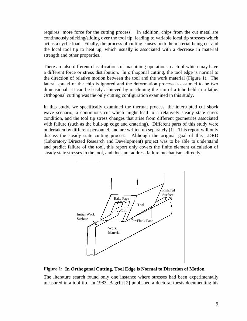
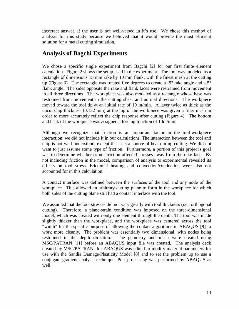
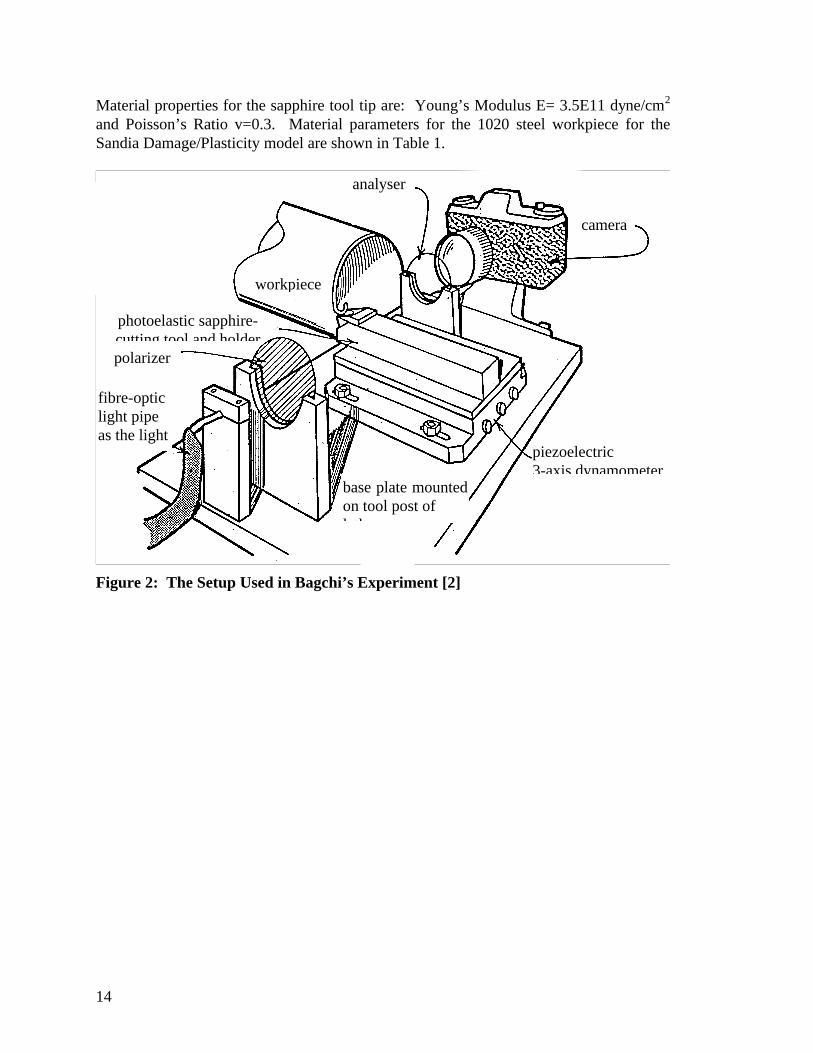
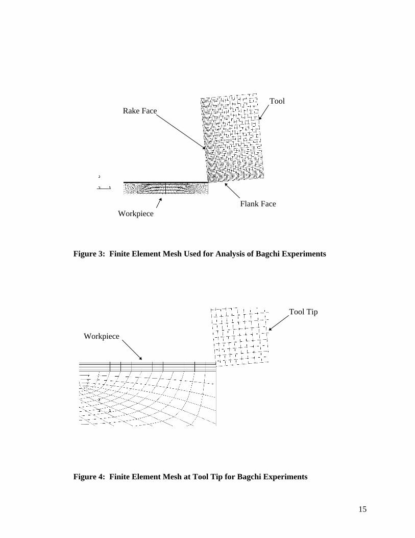
We chose a specific single experiment from Bagchi [2] for our first finite elementcalculation. Figure 2 shows the setup used in the experiment. The tool was modeled as arectangle of dimensions 15 mm rake by 10 mm flank, with the finest mesh at the cuttingtip (Figure 3). The rectangle was rotated five degrees to create a -5° rake angle and a 5°flank angle. The sides opposite the rake and flank faces were restrained from movementin all three directions. The workpiece was also modeled as a rectangle whose base wasrestrained from movement in the cutting shear and normal directions. The workpiecemoved toward the tool tip at an initial rate of 10 m/min. A layer twice as thick as theuncut chip thickness (0.132 mm) at the top of the workpiece was given a finer mesh inorder to more accurately reflect the chip response after cutting (Figure 4). The bottomand back of the workpiece was assigned a forcing function of 10m/min.

Although we recognize that friction is an important factor in the tool-workpieceinteraction, we did not include it in our calculations. The interaction between the tool andchip is not well understood, except that it is a source of heat during cutting. We did notwant to just assume some type of friction. Furthermore, a portion of this project's goalwas to determine whether or not friction affected stresses away from the rake face. Bynot including friction in the model, comparison of analysis to experimental revealed itseffects on tool stress. Frictional heating and convection/conduction were also notaccounted for in this calculation.

A contact interface was defined between the surfaces of the tool and any node of theworkpiece. This allowed an arbitrary cutting plane to form in the workpiece for whichboth sides of the cutting plane still had a contact interface with the tool.

We assumed that the tool stresses did not vary greatly with tool thickness (i.e., orthogonalcutting). Therefore, a plane-strain condition was imposed on the three-dimensionalmodel, which was created with only one element through the depth. The tool was madeslightly thicker than the workpiece, and the workpiece was centered across the tool“width” for the specific purpose of allowing the contact algorithms in ABAQUS [9] towork more cleanly. The problem was essentially two dimensional, with nodes beingrestrained in the depth direction. The geometry and mesh were created usingMSC/PATRAN [11] before an ABAQUS input file was created. The analysis deckcreated by MSC/PATRAN for ABAQUS was edited to modify material parameters foruse with the Sandia Damage/Plasticity Model [8] and to set the problem up to use aconjugate gradient analysis technique. Post-processing was performed by ABAQUS aswell.

14

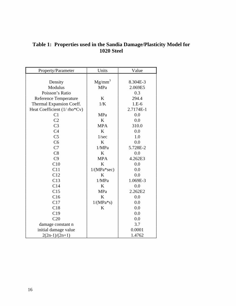
Material properties for the sapphire tool tip are: Young’s Modulus E= 3.5E11 dyne/cm2

and Poisson’s Ratio v=0.3. Material parameters for the 1020 steel workpiece for theSandia Damage/Plasticity model are shown in Table 1.

Figure 2: The Setup Used in Bagchi’s Experiment [2]

camera

piezoelectric3-axis dynamometer

base plate mountedon tool post ofl th

analyser

workpiece

photoelastic sapphire-cutting tool and holderpolarizer

fibre-opticlight pipeas the light

15

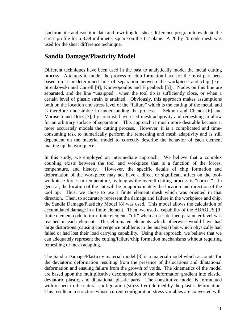
Figure 3: Finite Element Mesh Used for Analysis of Bagchi Experiments

Figure 4: Finite Element Mesh at Tool Tip for Bagchi Experiments

Tool

Workpiece

Workpiece

Tool Tip

Rake Face

Flank Face

16

Table 1: Properties used in the Sandia Damage/Plasticity Model for1020 Steel

Property/Parameter Units Value

Density Mg/mm3 8.304E-3Modulus MPa 2.069E5

Poisson’s Ratio 0.3Reference Temperature K 294.4

Thermal Expansion Coeff. 1/K 1.E-6Heat Coefficient (1/ rho*Cv) 2.7174E-1

C1 MPa 0.0C2 K 0.0C3 MPA 310.0C4 K 0.0C5 1/sec 1.0C6 K 0.0C7 1/MPa 5.728E-2C8 K 0.0C9 MPA 4.262E3C10 K 0.0C11 1/(MPa*sec) 0.0C12 K 0.0C13 1/MPa 1.069E-3C14 K 0.0C15 MPa 2.262E2C16 K 0.0C17 1/(MPa*s) 0.0C18 K 0.0C19 0.0C20 0.0

damage constant n 3.7initial damage value 0.0001

2(2n-1)/(2n+1) 1.4762

Comparison of Analysis to Bagchi's Experimental Data

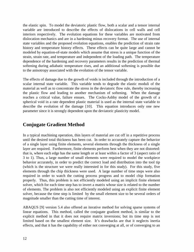
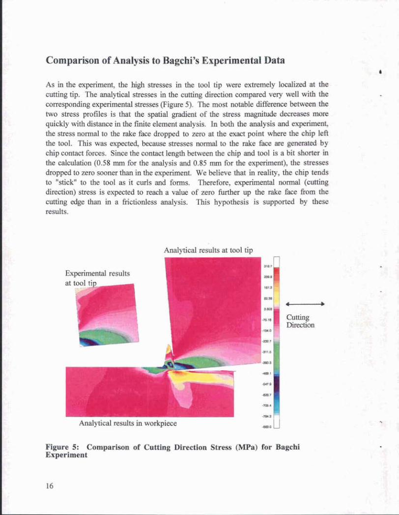
As in the experiment, the high stresses in the tool tip were extremely localized at the cutting tip. The analytical stresses in the cutting direction compared very well with the corresponding experimental stresses (Figure 5). The most notable difference between the two stress profiles is that the spatial gradient of the stress magnitude decreases more quickly with distance in the fmite element analysis. In both the analysis and experiment, the stress normal to the rake face dropped to zero at the exact point where the chip left the tool. This was expected, because stresses normal to the rake face are generated by chip contact forces. Since the contact length between the chip and tool is a bit shorter in the calculation (0.58 mm for the analysis and 0.85 mm for the experiment), the stresses dropped to zero sooner than in the experiment. We believe that in reality, the chip tends to "stick" to the tool as it curls and forms. Therefore, experimental normal (cutting direction) stress is expected to reach a value of zero fiuther up the rake face &om the cutting edge than in a frictionless analysis. This hypothesis is supported by these results.

Experimental resl at tool tin -

Analytical results at tool tip

m y t l c a results m workpiece

cutting Direction

Figure 5: Comparison of Cutting Direction Stress (MPa) for Bagchi Experiment

18

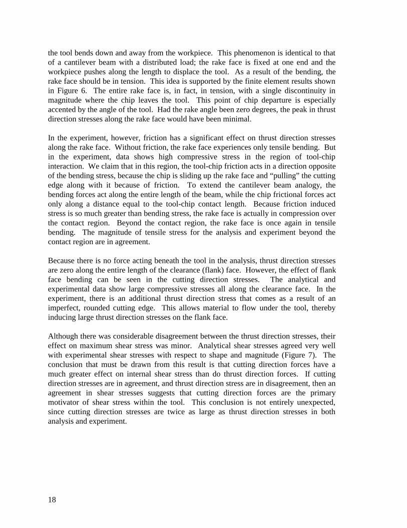
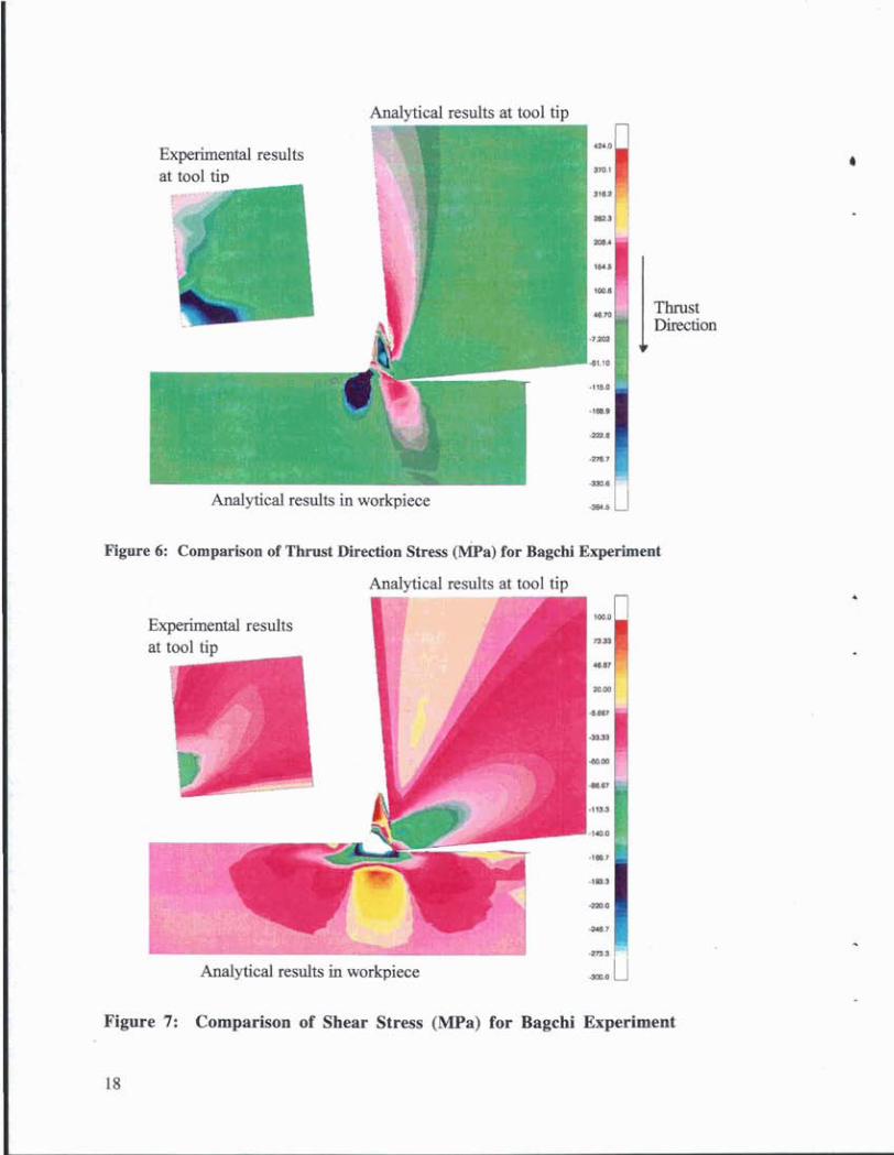
the tool bends down and away from the workpiece. This phenomenon is identical to thatof a cantilever beam with a distributed load; the rake face is fixed at one end and theworkpiece pushes along the length to displace the tool. As a result of the bending, therake face should be in tension. This idea is supported by the finite element results shownin Figure 6. The entire rake face is, in fact, in tension, with a single discontinuity inmagnitude where the chip leaves the tool. This point of chip departure is especiallyaccented by the angle of the tool. Had the rake angle been zero degrees, the peak in thrustdirection stresses along the rake face would have been minimal.

In the experiment, however, friction has a significant effect on thrust direction stressesalong the rake face. Without friction, the rake face experiences only tensile bending. Butin the experiment, data shows high compressive stress in the region of tool-chipinteraction. We claim that in this region, the tool-chip friction acts in a direction oppositeof the bending stress, because the chip is sliding up the rake face and “pulling” the cuttingedge along with it because of friction. To extend the cantilever beam analogy, thebending forces act along the entire length of the beam, while the chip frictional forces actonly along a distance equal to the tool-chip contact length. Because friction inducedstress is so much greater than bending stress, the rake face is actually in compression overthe contact region. Beyond the contact region, the rake face is once again in tensilebending. The magnitude of tensile stress for the analysis and experiment beyond thecontact region are in agreement.

Because there is no force acting beneath the tool in the analysis, thrust direction stressesare zero along the entire length of the clearance (flank) face. However, the effect of flankface bending can be seen in the cutting direction stresses. The analytical andexperimental data show large compressive stresses all along the clearance face. In theexperiment, there is an additional thrust direction stress that comes as a result of animperfect, rounded cutting edge. This allows material to flow under the tool, therebyinducing large thrust direction stresses on the flank face.

Although there was considerable disagreement between the thrust direction stresses, theireffect on maximum shear stress was minor. Analytical shear stresses agreed very wellwith experimental shear stresses with respect to shape and magnitude (Figure 7). Theconclusion that must be drawn from this result is that cutting direction forces have amuch greater effect on internal shear stress than do thrust direction forces. If cuttingdirection stresses are in agreement, and thrust direction stress are in disagreement, then anagreement in shear stresses suggests that cutting direction forces are the primarymotivator of shear stress within the tool. This conclusion is not entirely unexpected,since cutting direction stresses are twice as large as thrust direction stresses in bothanalysis and experiment.

Figore 6: Comparison of l l m s t

E e results at 1 :iv

, iece

1 results a

rn

Direction Stress (MPa) for Bagchi Experiment . . . . .

~nalytical results in workpie -Ymn U Figure 7: Comparison of Shear Stress (MPa) for Bagchi Experiment

20

Another parameter on which friction has a large effect is thrust force. Without friction,the only contribution to thrust force is the small vector component of force which is aresult of the chip contacting with the tilted tool. Had the rake angle been zero degrees,analytical thrust force would have averaged zero. Experimental thrust forces, on the otherhand, counteracted large frictional forces near the cutting edge. Resulting magnitudes offorce were on the order of 1200 N. Average analytical and experimental cutting forceswere in agreement to within 25%, with experimental forces being 1800 N and analyticalforces being 2200 N.

Other parameters were looked at numerically as part of this study, including rake angleand cutting speed, even though there were no experimental results to compare against.The internal memorandums of Reddy for the final Bagchi calculation and for theseparameter studies is included as Appendices A and B.

Sandia Experiments and Results

As the next step in the study, an experimental methodology was proposed for measuringlocalized stresses and temperatures in the tool tip, and a test matrix was proposed andimplemented. This test matrix involved carbide-tipped tools with 304L stainless steel and6061-T6 aluminum workpieces. We employed commercial cutting speeds which werefaster than for the Bagchi experiments. These measurement techniques and the testmatrix and results are described in detail in Reference [1].

Experimental data in the form of strain and temperature were taken at specific pointlocations in the tool. The technique used was to drill very small diameter access holesfrom the back of the tool, terminating at the desired gage locations. These locations werechosen based on the results of the analysis of the Bagchi experiment. Unfortunately, thesize of the strain gages was too large to capture more than an average of the cutting tipstress, which demonstrated an intense spatial gradient. We also could not consistentlylocate the gages as close to the cutting tip as needed in order to capture the peak stresses,due to the difficulty of working in the long, small diameter holes. Furthermore,problems in recording the data caused it to be truncated early in time (well before thermalsteady state was reached) for most experiments. Thus, the experimental data wascomposed of thermal data, strain at point locations, and tool forces, but needs to becarefully interpreted.

Two experiments were chosen as candidates for finite element calculations. Both had arake angle of 0 degrees, a flank angle of 5 degrees, a feed (cutting depth) of 0.0012 inch,and a cutting speed of 452 rpm (88.75 ips). The workpiece was 6061 T-6 aluminum forthe first and 304L stainless steel for the second.

21

Analyses of Sandia Experiments

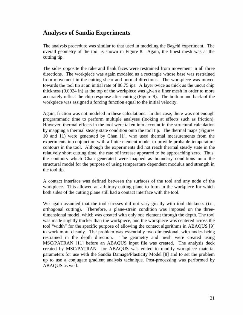
The analysis procedure was similar to that used in modeling the Bagchi experiment. Theoverall geometry of the tool is shown in Figure 8. Again, the finest mesh was at thecutting tip.

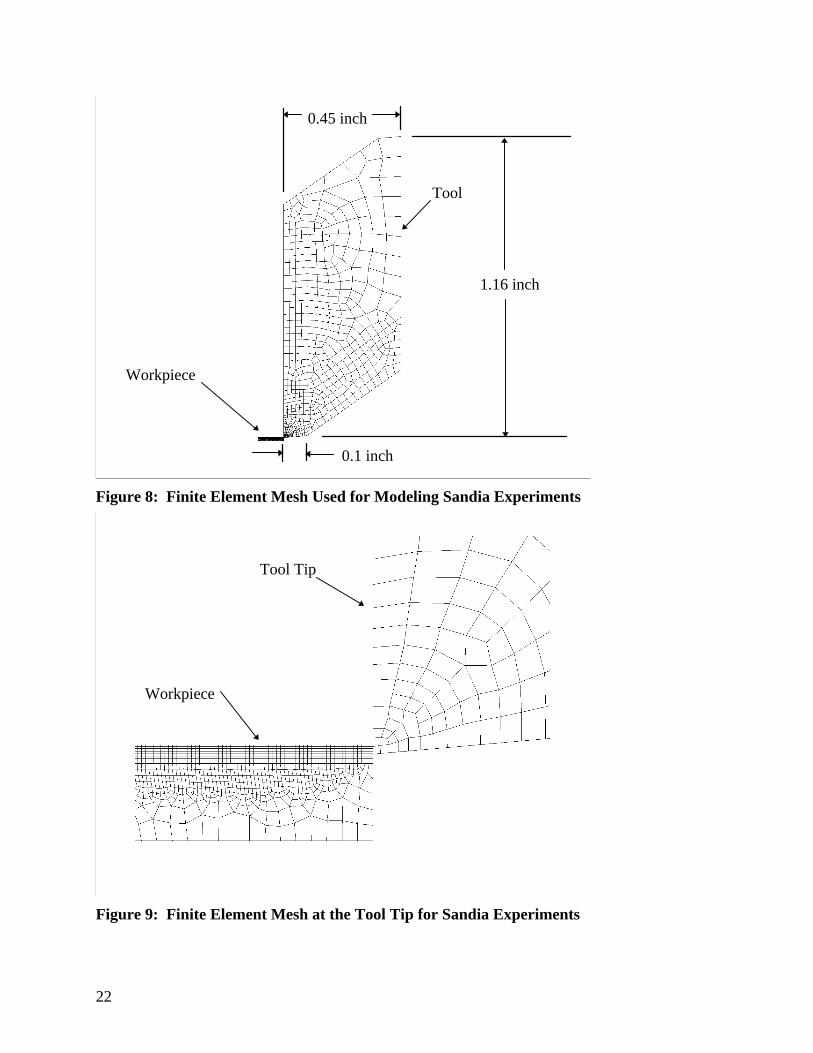
The sides opposite the rake and flank faces were restrained from movement in all threedirections. The workpiece was again modeled as a rectangle whose base was restrainedfrom movement in the cutting shear and normal directions. The workpiece was movedtowards the tool tip at an initial rate of 88.75 ips. A layer twice as thick as the uncut chipthickness (0.0024 in) at the top of the workpiece was given a finer mesh in order to moreaccurately reflect the chip response after cutting (Figure 9). The bottom and back of theworkpiece was assigned a forcing function equal to the initial velocity.

Again, friction was not modeled in these calculations. In this case, there was not enoughprogrammatic time to perform multiple analyses (looking at effects such as friction).However, thermal effects in the tool were taken into account in the structural calculationby mapping a thermal steady state condition onto the tool tip. The thermal maps (Figures10 and 11) were generated by Chan [1], who used thermal measurements from theexperiments in conjunction with a finite element model to provide probable temperaturecontours in the tool. Although the experiments did not reach thermal steady state in therelatively short cutting time, the rate of increase appeared to be approaching zero. Thus,the contours which Chan generated were mapped as boundary conditions onto thestructural model for the purpose of using temperature dependent modulus and strength inthe tool tip.

A contact interface was defined between the surfaces of the tool and any node of theworkpiece. This allowed an arbitrary cutting plane to form in the workpiece for whichboth sides of the cutting plane still had a contact interface with the tool.

We again assumed that the tool stresses did not vary greatly with tool thickness (i.e.,orthogonal cutting). Therefore, a plane-strain condition was imposed on the three-dimensional model, which was created with only one element through the depth. The toolwas made slightly thicker than the workpiece, and the workpiece was centered across thetool “width” for the specific purpose of allowing the contact algorithms in ABAQUS [9]to work more cleanly. The problem was essentially two dimensional, with nodes beingrestrained in the depth direction. The geometry and mesh were created usingMSC/PATRAN [11] before an ABAQUS input file was created. The analysis deckcreated by MSC/PATRAN for ABAQUS was edited to modify workpiece materialparameters for use with the Sandia Damage/Plasticity Model [8] and to set the problemup to use a conjugate gradient analysis technique. Post-processing was performed byABAQUS as well.

22

Figure 8: Finite Element Mesh Used for Modeling Sandia Experiments

Figure 9: Finite Element Mesh at the Tool Tip for Sandia Experiments

Tool

Workpiece

Workpiece

Tool Tip

1.16 inch

0.45 inch

0.1 inch

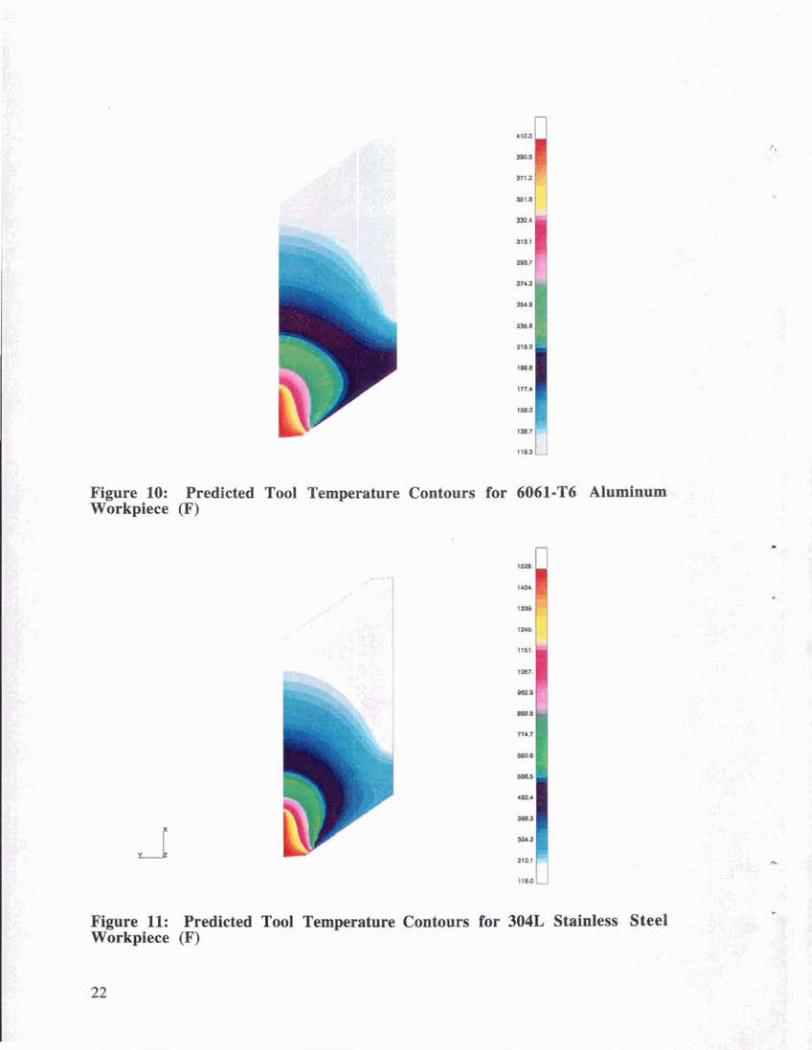
Figure 10: Predicted Workpiece (F)

Figure 11: Predicted Workpiece (F)

Tool

Tool

24

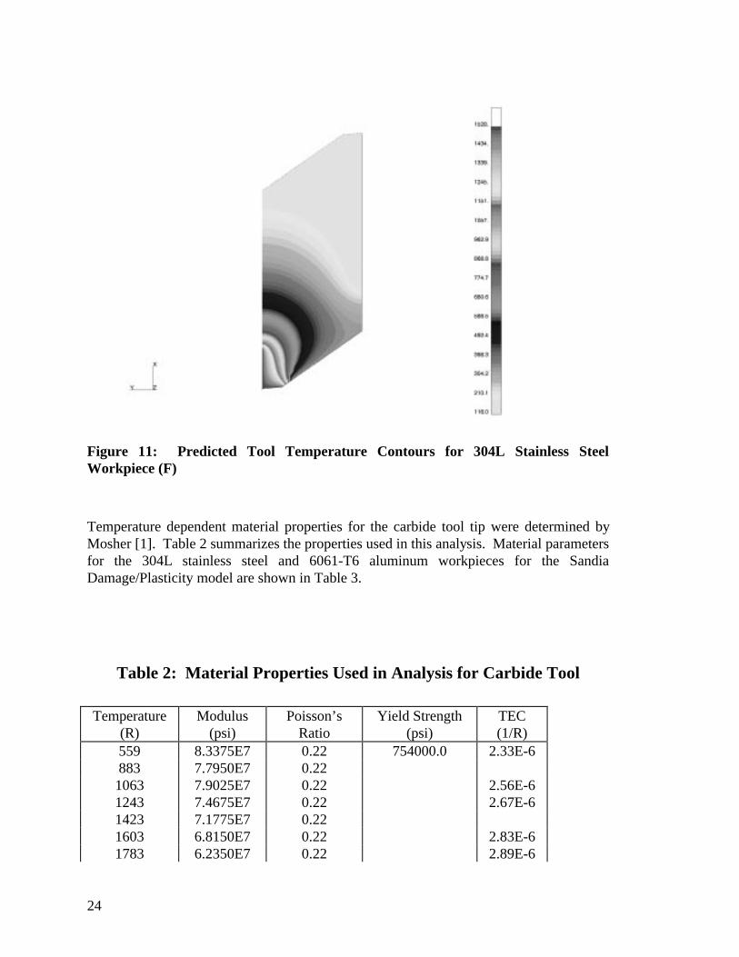
Figure 11: Predicted Tool Temperature Contours for 304L Stainless SteelWorkpiece (F)

Temperature dependent material properties for the carbide tool tip were determined byMosher [1]. Table 2 summarizes the properties used in this analysis. Material parametersfor the 304L stainless steel and 6061-T6 aluminum workpieces for the SandiaDamage/Plasticity model are shown in Table 3.

Table 2: Material Properties Used in Analysis for Carbide Tool

Temperature(R)

Modulus(psi)

Poisson’sRatio

Yield Strength(psi)

TEC(1/R)

559 8.3375E7 0.22 754000.0 2.33E-6883 7.7950E7 0.221063 7.9025E7 0.22 2.56E-61243 7.4675E7 0.22 2.67E-61423 7.1775E7 0.221603 6.8150E7 0.22 2.83E-61783 6.2350E7 0.22 2.89E-6

25

1963 5.5100E7 0.22 304500.02143 4.9300E7 0.222323 4.0600E7 0.22 145000.02503 58000.0

ρ = 0.098 lb/in3

26

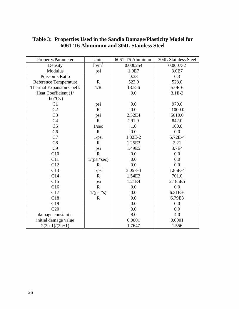
Table 3: Properties Used in the Sandia Damage/Plasticity Model for6061-T6 Aluminum and 304L Stainless Steel

Property/Parameter Units 6061-T6 Aluminum 304L Stainless SteelDensity lb/in3 0.000254 0.000732Modulus psi 1.0E7 3.0E7

Poisson’s Ratio 0.33 0.3Reference Temperature R 523.0 523.0

Thermal Expansion Coeff. 1/R 13.E-6 5.0E-6Heat Coefficient (1/

rho*Cv)0.0 3.1E-3

C1 psi 0.0 970.0C2 R 0.0 -1000.0C3 psi 2.32E4 6610.0C4 R 291.0 842.0C5 1/sec 1.0 100.0C6 R 0.0 0.0C7 1/psi 1.32E-2 5.72E-4C8 R 1.25E3 2.21C9 psi 1.49E5 8.7E4C10 R 0.0 0.0C11 1/(psi*sec) 0.0 0.0C12 R 0.0 0.0C13 1/psi 3.05E-4 1.85E-4C14 R 1.54E3 701.0C15 psi 1.21E4 2.185E5C16 R 0.0 0.0C17 1/(psi*s) 0.0 6.21E-6C18 R 0.0 6.79E3C19 0.0 0.0C20 0.0 0.0

damage constant n 8.0 4.0initial damage value 0.0001 0.0001

2(2n-1)/(2n+1) 1.7647 1.556

27

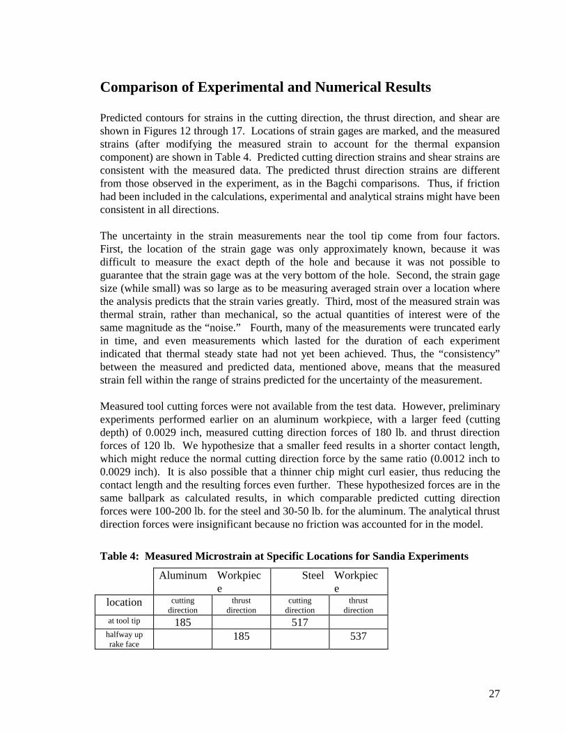
Comparison of Experimental and Numerical Results

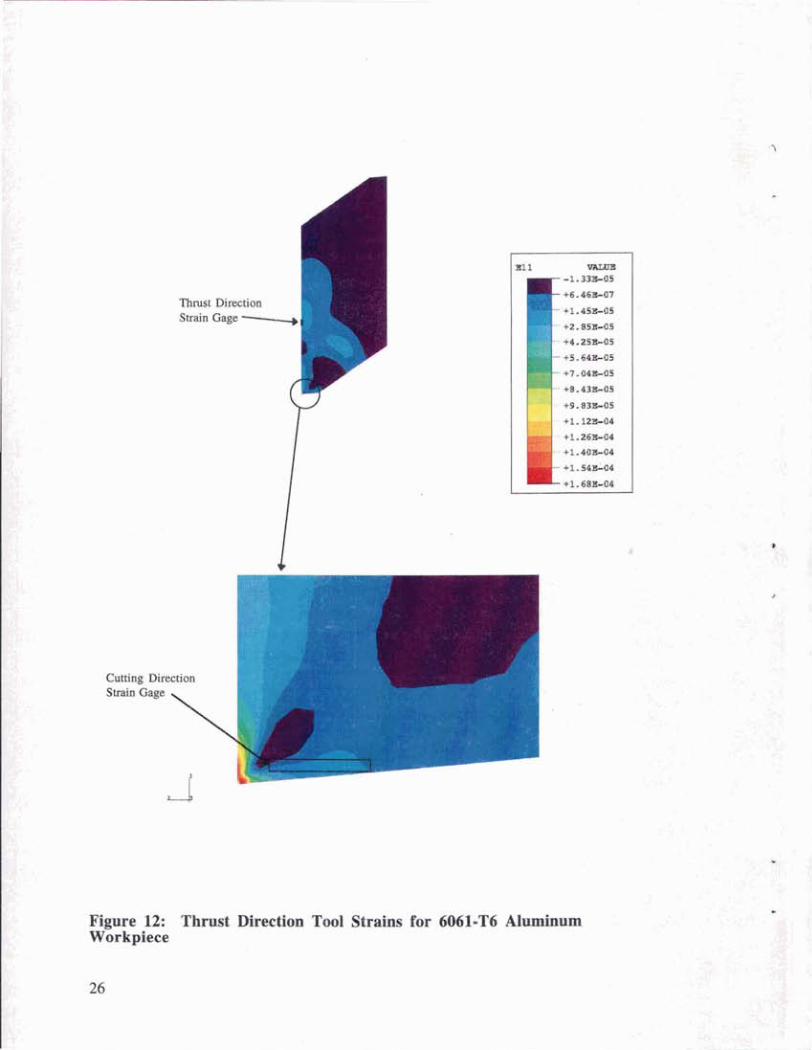
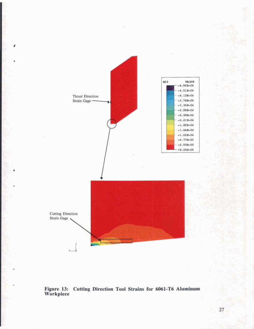
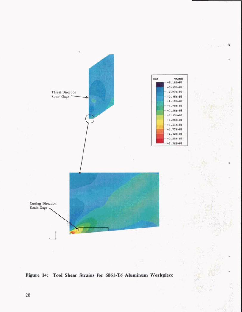
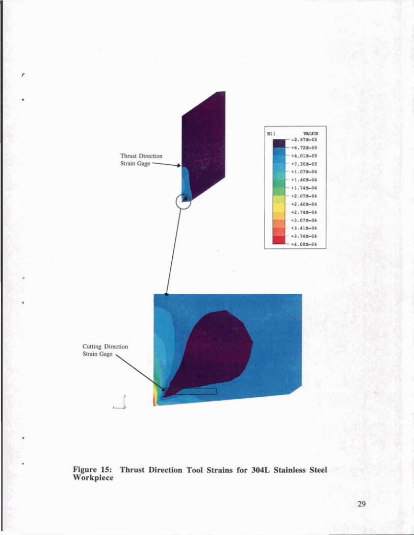
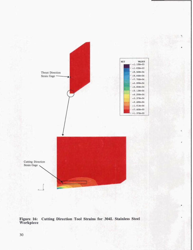
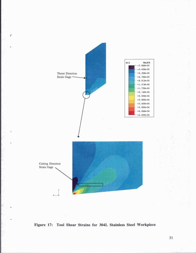
Predicted contours for strains in the cutting direction, the thrust direction, and shear areshown in Figures 12 through 17. Locations of strain gages are marked, and the measuredstrains (after modifying the measured strain to account for the thermal expansioncomponent) are shown in Table 4. Predicted cutting direction strains and shear strains areconsistent with the measured data. The predicted thrust direction strains are differentfrom those observed in the experiment, as in the Bagchi comparisons. Thus, if frictionhad been included in the calculations, experimental and analytical strains might have beenconsistent in all directions.

The uncertainty in the strain measurements near the tool tip come from four factors.First, the location of the strain gage was only approximately known, because it wasdifficult to measure the exact depth of the hole and because it was not possible toguarantee that the strain gage was at the very bottom of the hole. Second, the strain gagesize (while small) was so large as to be measuring averaged strain over a location wherethe analysis predicts that the strain varies greatly. Third, most of the measured strain wasthermal strain, rather than mechanical, so the actual quantities of interest were of thesame magnitude as the “noise.” Fourth, many of the measurements were truncated earlyin time, and even measurements which lasted for the duration of each experimentindicated that thermal steady state had not yet been achieved. Thus, the “consistency”between the measured and predicted data, mentioned above, means that the measuredstrain fell within the range of strains predicted for the uncertainty of the measurement.

Measured tool cutting forces were not available from the test data. However, preliminaryexperiments performed earlier on an aluminum workpiece, with a larger feed (cuttingdepth) of 0.0029 inch, measured cutting direction forces of 180 lb. and thrust directionforces of 120 lb. We hypothesize that a smaller feed results in a shorter contact length,which might reduce the normal cutting direction force by the same ratio (0.0012 inch to0.0029 inch). It is also possible that a thinner chip might curl easier, thus reducing thecontact length and the resulting forces even further. These hypothesized forces are in thesame ballpark as calculated results, in which comparable predicted cutting directionforces were 100-200 lb. for the steel and 30-50 lb. for the aluminum. The analytical thrustdirection forces were insignificant because no friction was accounted for in the model.

Table 4: Measured Microstrain at Specific Locations for Sandia Experiments

Aluminum Workpiece

Steel Workpiece

location cuttingdirection

thrustdirection

cuttingdirection

thrustdirection

at tool tip 185 517halfway uprake face

185 537

Cutting Direction Strain Gage

\

. , . . .~ .,,. . . - . . , :,". - ' . : . , . , I

1 : . . . . . , . . ,. . ~ . . . ;:. ' _ . I :, ,~ . . 7 . ::. 7: : ... . . ~ .. , . : -,: . : ; ,. . .. , . . .

. .. . b . ' , ,,,: . . , . ;- . . . . . ..'*)'. , . ' . -.-t:'';e ; .,

' . ;. ,I ' , . , . I . ~

. . 2 ,, . . .~ :. . , . 1

. . .

. .

..' . " . ... . . -. . . :

. I . '

' . ... . ~<..: . ~ r ; . . . . . . . . 8. : . . . .. . - . 'C. .,> ; . ;,:', ..::. , .. -.. ,~ . .

I : ' ... ., ' ,

~. . , . . .. .

, .. . : .. . , ~4. : +:i. ., . . . , ... .. . ,;:.* , . ~ . . . , - ,,.. ,?: , .I . ,' :

;: ,# , , , , -. ,

. .~ ' ' - . : , g $ : ; . < & . , ' - 2 ,

, < . . . - . . ;< . - r . ' .

Figure 12: Thrust Direction Tool Strains for 6061-T6 Aluminum Workpiece

26

Thnrst Direction Strain Gage -

Figure 13: Cutting Direction Tool Workpiece

Thtust Direction Shain Gage -

Tool Shear Strains for

Thrust Direction

Stmi" Gage -~

Cutting Direction

Figure 15: Workpiece

Thrust

Thrust Direction Strein Gage -

Cutting Direction

s-- \

Fipre 16: Cutting Direction Tool Strains for 304L Stainless Steel Workpiece

'Ihmst Directin* Seain Gage -

Flpre 17: Tool Shear Strains for 304L Stainless Steel Workpiece

34

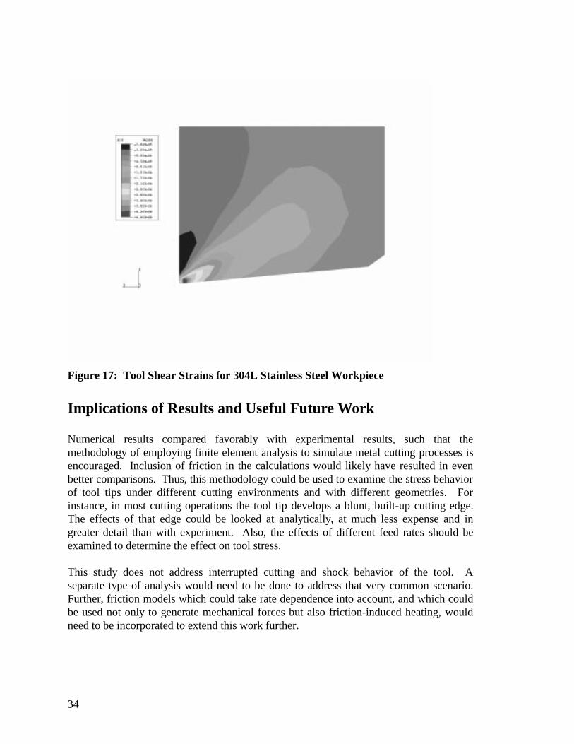
Figure 17: Tool Shear Strains for 304L Stainless Steel Workpiece

Implications of Results and Useful Future Work

Numerical results compared favorably with experimental results, such that themethodology of employing finite element analysis to simulate metal cutting processes isencouraged. Inclusion of friction in the calculations would likely have resulted in evenbetter comparisons. Thus, this methodology could be used to examine the stress behaviorof tool tips under different cutting environments and with different geometries. Forinstance, in most cutting operations the tool tip develops a blunt, built-up cutting edge.The effects of that edge could be looked at analytically, at much less expense and ingreater detail than with experiment. Also, the effects of different feed rates should beexamined to determine the effect on tool stress.

This study does not address interrupted cutting and shock behavior of the tool. Aseparate type of analysis would need to be done to address that very common scenario.Further, friction models which could take rate dependence into account, and which couldbe used not only to generate mechanical forces but also friction-induced heating, wouldneed to be incorporated to extend this work further.

35

Conclusions/Summary

The finite element method successfully predicted model stresses within sapphire andcarbide tools during slow and moderate speed machining. Comparison betweennumerical and experimental cutting direction and maximum shear stresses were excellent.Discrepancies between predicted and experimental thrust direction stresses wereexplained to be a function of friction that was not included in the numerical calculation.

Future FEM research should concentrate on understanding the tool-chip interaction zone,especially from a friction and plastic flow standpoint. Additionally, the effects oftemperature on tool wear should be investigated.

36

References

1. Hobson, W. T., Kistler, B. L., Chan, J., and Mosher, D., “Modeling and In-SituMechanical and Temperature Data for Cemented Carbide Tools Under RealisticMachining Conditions,” Sandia National Laboratories, To Be Published.

2. Bagchi, Amit. Photoelastic Stress Analysis in Machining Using Sapphire Tools.Ph.D. Thesis, Carnegie-Mellon University, Pittsburgh. UMI Dissertation Services,Ann Arbor, MI, 1984.

3. Timoschenko, S. P. and Goodier, J. N., Theory of Elasticity, McGraw-Hill BookCompany, New York, 1970.

4. Strenkowski, J. S. and Carroll, J. T., III, “A Finite Element Model of OrthogonalMetal Cutting,” J. Engrg. Ind., 107 (1985) 349-354.

5. Komvopoulos, K. and Erpenbeck, S. A., “Finite Element Modeling of OrthogonalMetal Cutting,” J. Engrg. Ind., 113 (1991) 253-267.

6. Sekhon, G. S. and Chenot, J. L., “Numerical Simulation of Continuous ChipFormation During Non-Steady Orthogonal Cutting,” Engineering Computations,10 (1993) 31-48.

7. Marusich, T. D., and Ortiz, M., “Modelling and Simulation of High-SpeedMachining,” Int. J. Num. Meth. Eng., TBP.

8. Bammann, D. J., Chiesa, M. L., McDonald, A., Kawahara, W. A., Dike, J. J., andRevelli, V. D., “Prediction of Ductile Failure in Metal Structures,” AMD, 107,(1990), 7-12.

9. Hibbitt, Karlsson and Sorensen, ABAQUS/Explicit User’s Manual, Version 5.4,1994.

10. Cocks, C. F. and Ashby, M. G., “Intergranular Fracture During Power-Law CreepUnder Multiaxial Stresses,” Metal Science, Aug-Sept, (1980), 395-402.

11. MSC/PATRAN, MacNeal-Schwendler Corp., (1996).

37

Appendix A: Internal Memorandum of Finite ElementCalculations of Bagchi [2] Experiment

38

Appendix B: Internal Memorandum of Finite ElementAnalysis Parameter Study Based on Experiments by Bagchi [2]

UNLIMITED RELEASE

Initial Distribution

Professor Paul WrightUniversity of California at BerkeleyDept. of Mechanical EngineeringBerkeley, CA 94720

Professor Dave DornfeldUniversity of California at BerkeleyDept. of Mechanical EngineeringBerkeley, CA 94720

Sandia Internal:

MS0188 4523 D. L. ChavezMS9007 8400 R. C. Wayne, Attn: MS9105 8419 H. H. HiranoMS9042 8742 M. R. BirnbaumMS9042 8743 Mike ChiesaMS9042 8743 Jay DikeMS9042 8742 Jim HandrockMS9042 8743 Mark HorstemeyerMS9042 8742 Paul JinMS9042 8742 Y. R. KanMS9042 8746 W. E. KawaharaMS9042 8742 B. L. Kistler (2)MS9042 2271 A. McDonaldMS9042 8742 Vera RevelliMS9042 8742 Jennifer RoblesMS9042 8742 Arlene SchauerMS9042 8742 K. V. TrinhMS9042 8742 L. E. VoelkerMS9042 8742 Larry WeingartenMS9105 8412 Jennifer ChanMS9105 8419 Bill HobsonMS9161 8716 K. L. WilsonMS9161 8717 W. G. WolferMS9402 8715 G. J. ThomasMS9403 8712 M. I. BaskesMS9403 8713 J. C. F. WangMS9405 8743 Doug BammannMS9405 8700 M. T. Dyer

39

MS9405 8240 Calvin KingMS9405 8743 P. E. NielanMS9420 8200 L. A. West, Attn: MS9430 8204 L. N. Tallerico

MS9430 8240 A. J. West

MS9021 8815 Technical Communications Department, for OSTI (10)MS9021 8815 Technical Communications Department/Technical Library, MS 0899, 4414MS0899 4414 Technical Library (4)MS9018 8940-2 Central Technical Files (3)