Finite DeformationsFrom statics and kinematics to finite elements

Matthieu Mazière1, Jacques Besson1, Samuel Forest1

1Mines ParisTech

March 11, 2013

Outline

Notations

scalar a avector a ai2nd order tensor a∼ aij4th order tensor a∼∼

aijkl

matrices aaaVoigt notation a∼→ aaa

V(a∼.b∼)

Products. c = a .b c = ai bi

c = a∼.b ci = aij bjc∼ = a∼.b∼ cij = aik bkj

: c = a∼ : b∼ c = aij bijc∼ = a∼∼

: b∼ cij = aijkl bkl

⊗ c∼ = a ⊗ b cij = ai bjc∼∼

= a∼⊗ b∼ cijkl = aij bkl

[Einstein convention]

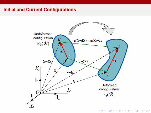
Initial and Current Configurations

Displacement and Transformation Gradient

• Displacement definitionu (X ) = x − X

• Displacement field around X

u (X + dX ) = u (X ) + du = u (X ) +∂u∂X

.dX

dx = dX + du =

„1∼+

∂u∂X

«.dX

• Transformation gradient

F∼ =∂x∂X

FiI =∂xi

∂XI

Objectivity and invariance

• Rigid body transformationx ′ = Q

∼(t).x + c (t)

• Quantities are objective if they are related by the rotation tensor as:

m′ = m

u ′ = Q∼

(t).u

T∼′ = Q

∼(t).T∼.Q

∼(t)T

• F∼ is not objective

F∼′ =

∂x ′

∂X=

∂x ′

∂x.∂x∂X

= Q∼

.F∼

• Quantities are invariant if they remain unchanged by the transformation

m′ = m, u ′ = u , T∼′ = T∼

• C∼ = F∼T .F∼ is invariant

C∼′ = F∼

′T .F∼′ = F∼

T .Q∼

T .Q∼

.F∼ = C∼

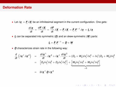
Deformation Rate

• Let δx = F∼.δX be an infinitesimal segment in the current configuration. One gets:

dδxdt

=dF∼.δX

dt=

dF∼dt

.δX = F∼.δX = F∼.F∼−1.δx = L∼.δx

• L∼ can be separated into symmetric (D∼) and an skew-symmetric (W∼ ) parts:

L∼ = F∼.F∼−1 = D∼ + W∼

• D∼ characterizes strain rate in the following way:

ddt

“δx 1.δx 2

”=

dδx 1

dt.δx 2 + δx 1.

dδx 2

dt= (Dij + Wij )δx1

j δx2i + δx1

i (Dij + Wij )δx2j

=hDijδx1

j δx2i + Dijδx1

i δx2j

i+hWijδx1

j δx2i + Wijδx1

i δx2j

i| z

=0

= 2δx 1.D∼.δx 2

Objectivity ?

• For a transformation such that: F∼′ = Q

∼(t).F∼

L∼′ = F∼

′.F∼′−1 = (Q

∼.F∼ + Q

∼.F∼).F∼

−1.Q∼−1

= Q∼

.Q∼

T + Q∼

.(D∼ + W∼ ).Q∼

T Q∼−1 = QT

= Q∼

.D∼.Q∼

T + Q∼

.Q∼

T + Q∼

.W∼ .Q∼

T

= D∼′ + W∼

′

• With

D∼′ = Q

∼.D∼.Q

∼T

W∼′ = Q

∼.W∼ .Q

∼T + Q

∼.Q∼

T

• Note that Q∼

.Q∼

T is skew-symmetric as:

Q∼

.Q∼

T = 1∼ ⇒ Q∼

.Q∼

T + Q∼

.Q∼

T= 0∼

• Only D∼ is objective

Polar Decomposition

• The deformation gradient F∼ can be decomposed, using the polar decompositiontheorem, into a product of two second-order tensors

F∼ = R∼.U∼ = V∼.R∼FiJ = RiK UKJ = Vik RkJ

with (R∼ rotation tensor)

R∼.R∼T = 1∼ U∼ = U∼

T V∼ = V∼T U∼ = R∼

T .V∼.R∼

Volume variation

• Jacobian of the transformation

J = det F∼ =VV0

> 0

• so that: ZΩ• dΩ =

ZΩ0

• JdΩ0

• Constant volume transformation means

J = 1

Deformation Tensors and Strain Measures

• Several rotation-independent symmetric deformation tensors are used inmechanics.

• Right Cauchy-Green deformation tensor [Lagrangian tensor]

C∼ = F∼T.F∼ = U∼

2 CIJ = F TIk FkJ = FkIFkJ

• Left Cauchy-Green deformation tensor [Eulerian tensor]

B∼ = F∼.F∼T = V∼

2 Bij = FiK F TKj = FiK FKj

• Additional selective rules for strain measures• Symmetric and dimensionless• Objective or invariant• Must be 0∼ for F∼ = 1∼• Must correspond to the small deformation theory for a first order Taylor expansion with

respect to F∼

Green-Lagrange E∼ =12

`C∼ − 1∼

´=

12

“U∼

2 − 1∼”

Biot strain tensor E∼Biot = U∼ − 1∼

Logarithmic strain tensor E∼log = log U∼

Principal stretches: λi

• U∼ and V∼ have the same eigenvalues λi and can be expressed as:

U∼ =3X

i=1

λi N i ⊗ N i V∼ =3X

i=1

λi n i ⊗ n i

• so that:

C∼ =3X

i=1

λ2i N i ⊗ N i B∼ =

3Xi=1

λ2i n i ⊗ n i

• One has:

V∼ = R∼.U∼.R∼T =

3Xi=1

λi (R∼.N i )⊗ (R∼.N i )

• Note also that:∂λi

∂C∼=

12λi

N i ⊗ N i

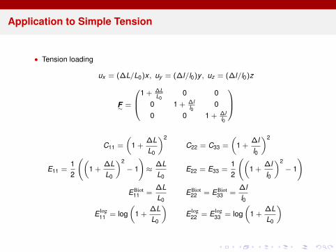
Application to Simple Tension

• Tension loading

ux = (∆L/L0)x , uy = (∆l/l0)y , uz = (∆l/l0)z

F∼ =

0B@1 + ∆LL0

0 00 1 + ∆l

l00

0 0 1 + ∆ll0

1CA

C11 =

„1 +

∆LL0

«2C22 = C33 =

„1 +

∆ll0

«2

E11 =12

„1 +

∆LL0

«2− 1

!≈

∆LL0

E22 = E33 =12

„1 +

∆ll0

«2− 1

!

EBiot11 =

∆LL0

EBiot22 = EBiot

33 =∆ll0

E log11 = log

„1 +

∆LL0

«E log

22 = E log33 = log

„1 +

∆LL0

«

Application to Simple Shear

• Simple shear

F∼ =

0@1 γ 00 1 00 0 1

1A C∼ =

0@1 γ 0γ γ2 + 1 00 0 1

1A B∼ =

0@1 + γ2 γ 0γ 1 00 0 1

1A = R∼.C∼.R∼T

• J = det F∼ = 1• R∼ has the form

R∼ =

0@cos θ − sin θ 0sin θ cos θ 0

0 0 1

1A → θ = − arctan γ/2

• Finally

U∼ = R∼T .F∼ =

0BBBB@2p

4 + γ2

γp4 + γ2

0

γp4 + γ2

γ2p4 + γ2

+2p

4 + γ20

0 0 1

1CCCCA• First order Taylor expansion

C∼ =

0@1 γ 0γ 1 00 0 1

1A = U∼ → θ = −γ

2

Outline

True or Cauchy stress tensor

• T∼ (Tij ) defined by df = T∼.n dS• Stress measure using the current configuration• Velocity gradient

L∼ = F∼.F∼−1 = D∼ + W∼

• Workw =

ZΩ

T∼ : D∼ dΩ

• Kirchhoff stress

w =

ZΩ

T∼ : D∼ dΩ =

ZΩ0

JT∼ : D∼ dΩ0 =

ZΩ0

K∼ : D∼ dΩ0

K∼ = JT∼ Kij = JTij

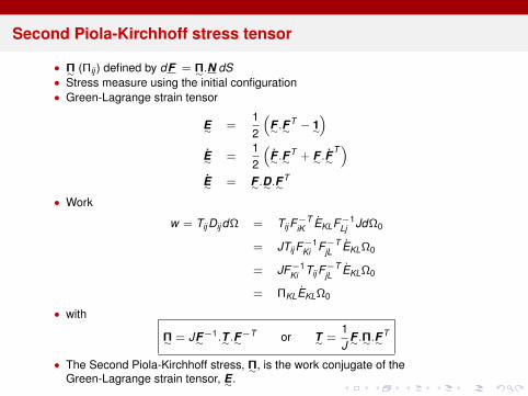
Second Piola-Kirchhoff stress tensor

• Π∼ (Πij ) defined by dF = Π∼.N dS• Stress measure using the initial configuration• Green-Lagrange strain tensor

E∼ =12

“F∼.F∼

T − 1∼”

E∼ =12

“F∼.F∼

T + F∼.F∼T”

E∼ = F∼.D∼.F∼T

• Work

w = Tij Dij dΩ = Tij F−TiK EKLF−1

Lj JdΩ0

= JTij F−1Ki F−T

jL EKLΩ0

= JF−1Ki Tij F

−TjL EKLΩ0

= ΠKLEKLΩ0

• with

Π∼ = JF∼−1.T∼.F∼

−T or T∼ =1J

F∼.Π∼.F∼T

• The Second Piola-Kirchhoff stress, Π∼, is the work conjugate of theGreen-Lagrange strain tensor, E∼.

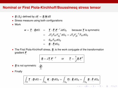
Nominal or First Piola-Kirchhoff/Boussinesq stress tensor

• S∼ (Sij ) defined by df = S∼.N dS• Stress measure using both configurations• Work

w = T∼ : D∼dΩ = T∼ : F∼.F∼−1JdΩ0 because T∼ is symmetric

= JTij FiK F−1Kj dΩ0 = JTij F

−TjK FiK dΩ0

= SiK FiK dΩ0

= S∼ : F∼dΩ0

• The First Piola-Kirchhoff stress, S∼, is the work conjugate of the transformationgradient F∼

S∼ = JT∼.F∼−T or T∼ =

1J

S∼.F∼T

• S∼ is not symmetric

• Finally ZΩ

T∼ : D∼ dΩ =

ZΩ0

K∼ : D∼ dΩ0 =

ZΩ0

Π∼ : E∼ dΩ0 =

ZΩ0

S∼ : F∼ dΩ0

Interpretation of the various stress measures: tensile test

• Transformation gradient — Cauchy stress [final configuation]

F∼ =

0@F‖ 0 00 F⊥ 00 0 F⊥

1A J = F‖F 2⊥ T∼ =

0@T 0 00 0 00 0 0

1A• Kirchhoff stress

K∼ = JT∼ K = F‖F 2⊥T K = T for incompressible materials

• Second Piola-Kirchhoff

Π∼ = JF∼−1.T∼.F∼

−T Π =F 2⊥

F‖T for incompressible materials Π =

1F 2‖

T

• First Piola-Kirchhoff stress

S∼ = JT∼.F∼−T S =

1F‖

T ≈ engineering stress

Jaumann derivative of a vector

• Constitutive laws require objectives rates• W∼ is not objective

W∼′ = Q

∼.W∼ .Q

∼T + Q

∼.Q∼

T

• so that:

Q∼

= W∼′.Q∼− Q∼

.W∼

Q∼

T= −Q

∼T .W∼

′ + W∼ .Q∼

T

• For an objective displacement vector u ′ = Q∼

.u , one gets:

u ′ = Q∼

.u + Q∼

.u = (W∼′.Q∼− Q∼

.W∼ ).u + Q∼

.u = W∼′.u ′ − Q

∼.W∼ .u + Q

∼.u

• So that:u ′ −W∼

′.u ′ = Q∼

.(u −W∼ .u )

• This allows to define an objective derivative of vectors (Jaumann rate):

u J = u −W∼ .u

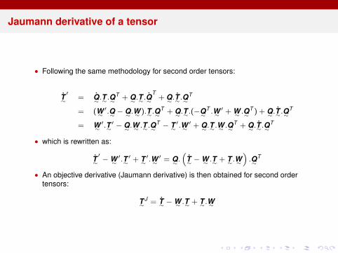
Jaumann derivative of a tensor

• Following the same methodology for second order tensors:

T∼′

= Q∼

.T∼.Q∼

T + Q∼

.T∼.Q∼

T+ Q∼

.T∼.Q∼

T

= (W∼′.Q∼− Q∼

.W∼ ).T∼.Q∼

T + Q∼

.T∼.(−Q∼

T .W∼′ + W∼ .Q

∼T ) + Q

∼.T∼.Q

∼T

= W∼′.T∼

′ − Q∼

.W∼ .T∼.Q∼

T − T∼′.W∼

′ + Q∼

.T∼.W∼ .Q∼

T + Q∼

.T∼.Q∼

T

• which is rewritten as:

T∼′ −W∼

′.T∼′ + T∼

′.W∼′ = Q

∼.“

T∼ −W∼ .T∼ + T∼.W∼”

.Q∼

T

• An objective derivative (Jaumann derivative) is then obtained for second ordertensors:

T∼J = T∼ −W∼ .T∼ + T∼.W∼

Stress rates - Truesdell stress rate

• Recall the relation between the Cauchy and the second Piola-Kirchhoff stress:

T∼ =1J

F∼.Π∼.F∼T Π∼ = JF∼

−1.T∼.F∼−T

• As Π∼ is invariant the following stress rate will be objective (it corresponds to thetransport of the rate of the second Piola-Kirchhoff stress):

T∼ =

1J

F∼.Π∼.F∼T 6= T∼

• Noting that:

Π∼ = JF∼−1.T∼.F∼

−T + JF∼−1

.T∼.F∼−T + JF∼

−1.T∼.F∼−T + JF∼

−1.T∼.F∼−T

• So that:T∼ =

JJ

T∼ + F∼.F∼−1

.T∼ + T∼.F∼−T

.F∼T + T∼

• Note thatddt

(F∼.F∼−1) = 0∼= F∼.F∼

−1 + F∼.F∼−1

• so thatF∼.F∼

−1= −L∼ and F∼

−T.F∼

T = −L∼T

• One also hasJ/J = TrL∼

• Finally, one obtains the Truesdell stress rate

T∼ = TrL∼T∼ − L∼.T∼ − T∼.L∼

T + T∼

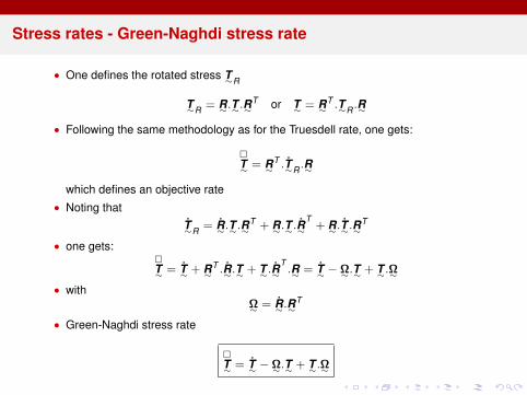
Stress rates - Green-Naghdi stress rate

• One defines the rotated stress T∼R

T∼R = R∼.T∼.R∼T or T∼ = R∼

T .T∼R .R∼

• Following the same methodology as for the Truesdell rate, one gets:

T∼ = R∼

T .T∼R .R∼

which defines an objective rate• Noting that

T∼R = R∼.T∼.R∼T + R∼.T∼.R∼

T+ R∼.T∼.R∼

T

• one gets:T∼ = T∼ + R∼

T .R∼.T∼ + T∼.R∼T.R∼ = T∼ −Ω∼.T∼ + T∼.Ω∼

• withΩ∼ = R∼.R∼

T

• Green-Naghdi stress rate

T∼ = T∼ −Ω∼.T∼ + T∼.Ω∼

Outline

Constitutive equations : hyperelasticity

• Hyperelasticity is often used for elastomers• One first defines a strain energy density function W which depends on C∼• For isotropic materials, W only depends on the invariants of C∼

I1 = TrC∼

I2 =12

“(TrC∼)2 − TrC∼.C∼

”I3 = det C∼ for incompressible materials: I3 = 1

J = det F∼ I3 = J2

• The second Piola-Kirchhoff stress is then given by:

Π∼ =∂W∂E∼

= 2∂W∂C∼

• Mooney-Rivlin lawW = C1(I1 − 3) + C2(I2 − 3)

• Ogden

W (λ1, λ2, λ3) =NX

p=1

µp

αp

“λ

αp1 + λ

αp2 + λ

αp3 − 3

”

Constitutive equations : hypo-elasticity

• The constitutive equations are written in a rate form relating any objective stressrate to the deformation rate D∼:

T∼J ,

T∼,

T∼, · · · = Λ∼∼

: D∼

• These constitutive equations may be path dependent . . . not physical

Constitutive equations : F∼e.F∼

p decomposition

• One assume an elastic (F∼e) / plastic (F∼

p) transformation decomposition

F∼ = F∼e.F∼

p

• The decomposition defines an intermediate state :

• The deformation rate is given by:

L∼ = F∼.F∼−1 = F∼

e.F∼

e−1 + F∼e.F∼

p.F∼

p−1.F∼e−1 = L∼

e + F∼e.L∼

p.F∼e−1

• Express L∼p = D∼

p + W∼p

Examples

• Isotropic von Mises plasticity

D∼p =

32

pT∼′

T ′eqW∼

p = 0∼

• Crystal plasticity

D∼p =

Xs

γs (m s ⊗ n s + m s ⊗ n s) W∼p =

Xs

γs (m s ⊗ n s −m s ⊗ n s)

γs = γs(T∼ : (m s ⊗ n s))

Constitutive equations : corotational formulations

• Polar formulation• The constitutive equation is expressed between the rotated stress T∼R

= R∼.T∼.R∼T and

any stress measure constructed using U∼• The small strain formalism can be used for the constitutive equations• The corresponding objective stress stress rate is the Green-Naghdi rate.

• Rotate formulation• The constitutive equations are expressed using: T∼Q

= Q∼.T∼.Q∼T where Q∼ is obtained

integrating the following equation:Q∼ = W∼ .Q∼

• The corresponding strain tensor is:

ε∼Q=

ZtdD∼

• The constitutive equations then relate:

T∼Q= f (ε∼Q

) small strain formalism

• The corresponding objective stress stress rate is the Jaumann rate.

Outline

Finite element formulation: small strain

• Internal virtual power (one finite element):ZΩ

σ∼ : δε∼dΩ =

ZΩ

“BBBT

ε .σσσ”

.uuun dΩ ≡ FFF i .uuun

• Internal elementary force:

FFF i =

ZΩ

BBBTε .σσσ dΩ

• Elementary stiffness matrix

KKK e =

ZΩ

BBBTε .

∂σσσ

∂εεε.BBBε dΩ

Finite element formulation: total lagrangian

• Internal virtual power (one finite element):ZΩ0

Π∼ : δE∼ dΩ0 =

ZΩ0

ΠΠΠ.δEEE dΩ0 ≡ FFF i .uuun

• Transformation gradient

FFF = 111 + eee = 111 + BBBFX .uuun δFFF = BBBFX .δuuun

• Green-Lagrange strain:

E∼ =12

“F∼

T .F∼ − 1∼”

=12(e∼+ e∼

T ) +12

e∼T .e∼ = ε∼X +

12

e∼T .e∼ ⇒

δE∼ = δε∼X +12

δe∼T .e∼+

12

e∼T .δe∼

• Using Voigt notations

δEEE = δεεεX +12

MMML(e∼T ).δeee +

12

MMMR(e∼).δeeeT = δεεεX +12

MMML(e∼T ).δeee +

12

MMMR(e∼).TTT .δeee

δEEE = δεεεX +12

(111 + TTT ) .MMML(e∼T ).δeee =

„BBBεX +

12

(111 + TTT ) .MMML(e∼T ).BBBFX

«.δuuun ≡ BBBEX .δuuun

using MMMR (a∼).TTT = TTT .MMML(a∼T )

• The internal forces are then computed as:

FFF i =

ZΩ0

BBBTEX .ΠΠΠ dΩ0

• The elementary stiffness matrix is then computed as:

KKK e =∂FFF i

∂uuun

• The product BBBTEX .ΠΠΠ can be rewritten as:

BBBTEX .ΠΠΠ = BBBT

εX .ΠΠΠ +12

BBBTFX .MMML(e∼). (111 + TTT ) .ΠΠΠ Π∼ is symmetric

= BBBTεX .ΠΠΠ + BBBT

FX .MMML(e∼).ΠΠΠ

= BBBTεX .ΠΠΠ + BBBT

FX .MMMR(Π∼).eee

• So that

KKK e =

ZΩ0

„BBBT

EX .∂ΠΠΠ

∂EEE.BBBEX + BBBT

FX .MMMR(Π∼).BBBFX

«dΩ0

Finite element formulation: updated lagrangian

• Internal virtual power (one finite element):ZΩ

σ∼ : δε∼dΩ =

ZΩ

σσσ.δεεε dΩ ≡ FFF i .uuun

• The same method as before applies considering that σ∼ is the secondPiola-Kirchhoff stress at time t expressed in the reference frame at t (and not att0). In that case, one gets:

FFF i =

ZΩ

BBBεx .σσσ dΩ

and

KKK e =

ZΩ

„BBBT

εx .∂σσσ

∂εεε.BBBεx + BBBT

Fx .MMMR(σ∼).BBBFx

«dΩ