Finding Your Friends andFollowing Them to Where You Are

Adam SadilekDept. of Computer Science

University of RochesterRochester, NY, USA

sadilek@cs.rochester.edu

Henry KautzDept. of Computer Science

University of RochesterRochester, NY, USA

kautz@cs.rochester.edu

Jeffrey P. BighamDept. of Computer Science

University of RochesterRochester, NY, USA

jbigham@cs.rochester.edu

ABSTRACTLocation plays an essential role in our lives, bridging ouronline and offline worlds. This paper explores the interplaybetween people’s location, interactions, and their social tieswithin a large real-world dataset. We present and evaluateFlap, a system that solves two intimately related tasks: linkand location prediction in online social networks. For linkprediction, Flap infers social ties by considering patternsin friendship formation, the content of people’s messages,and user location. We show that while each component isa weak predictor of friendship alone, combining them re-sults in a strong model, accurately identifying the majorityof friendships. For location prediction, Flap implements ascalable probabilistic model of human mobility, where wetreat users with known GPS positions as noisy sensors ofthe location of their friends. We explore supervised and un-supervised learning scenarios, and focus on the efficiency ofboth learning and inference. We evaluate Flap on a largesample of highly active users from two distinct geographicalareas and show that it (1) reconstructs the entire friendshipgraph with high accuracy even when no edges are given;and (2) infers people’s fine-grained location, even when theykeep their data private and we can only access the locationof their friends. Our models significantly outperform currentcomparable approaches to either task.

Categories and Subject DescriptorsH.1.m [Information Systems]: Miscellaneous

General TermsAlgorithms, Experimentation, Human Factors

KeywordsLocation modeling, link prediction, social networks, machinelearning, graphical models, visualization, Twitter

Permission to make digital or hard copies of all or part of this work forpersonal or classroom use is granted without fee provided that copies arenot made or distributed for profit or commercial advantage and that copiesbear this notice and the full citation on the first page. To copy otherwise, torepublish, to post on servers or to redistribute to lists, requires prior specificpermission and/or a fee.WSDM’12, February 8–12, 2012, Seattle, Washingtion, USA.Copyright 2012 ACM 978-1-4503-0747-5/12/02 ...$10.00.

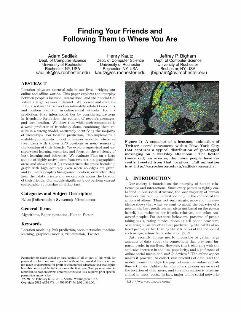
Figure 1: A snapshot of a heatmap animation ofTwitter users’ movement within New York Citythat captures a typical distribution of geo-taggedmessaging on a weekday afternoon. The hotter(more red) an area is, the more people have re-cently tweeted from that location. Full animationis at http://cs.rochester.edu/u/sadilek/research/.

1. INTRODUCTIONOur society is founded on the interplay of human rela-

tionships and interactions. Since every person is tightly em-bedded in our social structure, the vast majority of humanbehavior can be fully understood only in the context of theactions of others. Thus, not surprisingly, more and more ev-idence shows that when we want to model the behavior of aperson, the best predictors are often not based on the personherself, but rather on her friends, relatives, and other con-nected people. For instance, behavioral patterns of peopletaking taxis, rating movies, choosing cell phone providers,or sharing music are often best predicted by the habits of re-lated people, rather than by the attributes of the individualsuch as age, ethnicity, or education [3, 24].

Until recently, it was nearly impossible to gather largeamounts of data about the connections that play such im-portant roles in our lives. However, this is changing with theexplosive increase in the use, popularity, and significance ofonline social media and mobile devices.1 The online aspectmakes it practical to collect vast amounts of data, and themobile element bridges the gap between our online and of-fline activities. Unlike other computers, phones are aware ofthe location of their users, and this information is often in-cluded in users’ posts. In fact, major online social networks

1http://www.comscore.com/

are fostering location sharing. Twitter added an explicitGPS tag that can be specified for each tweet (AKA Twittermessage update) in early 2010 and is continually improvingthe location-awareness of its service. Google+, Facebook,FourSquare, and Gowalla allow people to share their loca-tion, and to “check-in” at venues. With Google Latitude andBliin, users can continually broadcast their location.

Thus, we now have access to colossal amounts of real-world data containing not just the text and images peoplepost, but also their location. Of course, these three datamodalities are not necessarily mutually independent. Forinstance, photos are often GPS-tagged and locations canalso be mentioned, or alluded to, in text.

While the information about users’ location and relation-ships is important to accurately model their behavior andimprove their experience, it is not always available. Thispaper explores novel techniques of inferring this latent in-formation from a stream of message updates. We presenta unified view on the interplay between people’s location,message updates, and their social ties on a large real-worlddataset. Our approaches are robust and achieve significantlyhigher accuracy than the best currently known methods,even in difficult experimental settings spanning diverse geo-graphical areas.

1.1 Significance of ResultsConsider the task of determining the exact geographic lo-

cation of an arbitrary user of an online social network. Ifshe routinely geo-tags her posts and makes them public, theproblem is relatively easy. However, suppose the locationinformation is hidden, and you only have access to publicposts by her friends. By leveraging social ties, our proba-bilistic location model—the first component of this work—infers where any given user is with high accuracy and finegranularity in both space and time even when the user keepshis or her posts private. Since this work shows that once wehave location information for some proportion of people, wecan infer the location of their friends, one can imagine doingthis recursively until the entire target population is covered.To our knowledge, no other work attempts to predict loca-tions in a comparably difficult setting.

The main power of our link prediction approach—the sec-ond major component of this work—is that it accurately re-constructs the entire friendship graph even when no “seed”ties are provided. Previous work either obtained very goodpredictions at the expense of large computational costs (e.g.,[28]), thereby limiting those approaches to very small do-mains, or sacrificed orders of magnitude in accuracy fortractability (e.g., [19, 7]). By contrast, we show that ourmodel’s performance is comparable to the most powerful re-lational methods applied in previous work [28], while at thesame time being applicable to large real-world domains withtens of millions (as opposed to hundreds) of possible friend-ships. Since our model leverages users’ locations, it not onlyencompasses virtual friendships, but also begins to tie themtogether with their real-life groundings.

Prediction of people’s location and social ties—especiallywhen considered together—has a number of important ap-plications. They range from improved local content withbetter social context, through increased security (both per-sonal and electronic) via detection of abnormal behavior tiedwith one’s location, to better organization of one’s relation-ships and connecting virtual friendships with the real-world.

We note that even when friends participate in the samesocial networking platform, their relationship may not beexposed—either because the connections are hidden or be-cause they have not yet connected online. Flap can alsohelp contain disease outbreaks [12]. Our model allows iden-tification of highly mobile individuals as well as their mostlikely meeting points, both in the past and in the future.These people can be subsequently selected for targeted treat-ment or preemptive vaccination. Given people’s inferred lo-cations, and limited resource budget, a decision-theoreticapproach can be used to select optimal emergency policy.Clearly, strong privacy concerns are tied to such applica-tions, as we discuss in the conclusions.

2. RELATED WORKRecent research in location-based reasoning explored

harnessing data collected on regular smart phones for mod-eling human behavior [10]. Specifically, they model indi-viduals’ general location from nearby cell towers and Blue-tooth devices at various times of day. Eagle et al. showthat predicting if a person is at home, at work, or some-place else can be achieved with more than 90% accuracy.Besides scalability and practicality—social network data ismuch more readily available than cell phone logs—our workdiffers in that we include dynamic relational features (loca-tion of friends), focus on a finer time granularity, and con-sider a substantially larger set of locations (hundreds peruser, rather than three). Additionally, the observations inour framework (people’s self-published locations) are signifi-cantly noisier and less regular than cell tower and Bluetoothreadings. Finally, our location estimation applies even in sit-uations, where the target people decide to keep their dataprivate.

Backstrom et al. predict the home address of Facebookusers based on provided addresses of one’s friends [2]. Anempirically extracted relationship between geographical dis-tance and the probability of friendship between pairs of usersis leveraged in order to find a maximum likelihood assign-ment of addresses to hidden users. The authors show thattheir method of localizing users is in general more accuratethan an IP address-based alternative. However, even theirstrongest approach captures only a single static home lo-cation for each user and the spatial resolution is low. Forexample, less than 50% of the users are localized within 10miles of their actual home. By contrast, we consider muchfiner temporal resolution (20 minute intervals) and achievesignificantly greater spatial precision, where up to 84% ofpeople’s exact dynamic location is correctly inferred.

Very recently, Cho et al. focus on modeling user locationin social networks as a dynamic Gaussian mixture, a gen-erative approach postulating that each check-in is inducedfrom the vicinity of either a person’s home, work, or is aresult of social influence of one’s friends [6]. By contrast,our location model is inherently discrete, which allows usto predict the exact location rather than a sample from agenerally high-variance continuous distribution; operates ata finer time granularity; and learns the candidate locationsfrom noisy data. Furthermore, our approach leverages thecomplex temporal and social dependencies between people’slocations in a more general, discrete fashion. We show thatour model outperforms that of Cho et al. in the experimentspresented below.

A number of geolocating applications demonstrate emerg-

ing privacy issues in this area. The most impactful ones arearguably Creepy2, ICanStalkU.com, and PleaseRobMe.com(currently disabled). The purpose of these efforts is to raiseawareness about the lack of location privacy in online socialnetworks. Given a username from an online social network,Creepy aggregates location information about the target in-dividual from her GPS-tagged posts and photos, and dis-plays it on a map. ICanStalkU.com scans public Twittertimeline, and extracts GPS metadata from uploaded pho-tos, which often reveal people’s current location withoutthem realizing it. PleaseRobMe.com used to extract peo-ple’s geographic check-ins that imply they are not at homeand therefore vulnerable to burglaries.

However, all these applications work only with publiclyavailable data. By contrast, this paper shows that we caninfer people’s precise location even when they keep theirdata private, as long as some of their friends post their loca-tion publicly. Therefore, simply turning off the geolocationfeatures of your phone—which may seem to be a reliableway to keep your whereabouts secret—does not really pro-tect your privacy unless your friends turn theirs off as well.

While our work concentrates on Twitter users, recent re-search shows that the predictability of human mobility re-mains virtually unchanged across a number of demographi-cal attributes such as age and gender [27]. This strongly sug-gests that our approach achieves similar accuracy for othergeographical areas and different samples of users. Finally,we note that although it has been shown that possibly asmany as 34% of accounts provide either wrong or mislead-ing symbolic (e.g., city, state) location information in theirprofiles, our work is largely shielded from this phenomenonsince we focus only on raw GPS data that can be more read-ily verified and is not fed into a geocoder [15].

The problem of link prediction has been studied in alarge number of domains and contexts; here we mention theones that are most relevant to our work. Liben-Nowell etal. models the evolution of a graph solely from its topo-logical properties [19]. The authors evaluate a number ofmethods of quantifying the probability of a link in largegraphs, and conclude that while no single technique is sub-stantially better than the rest, their models outperform arandom predictor by a significant margin. This shows thatthere is important information to be mined from the graphstructure alone.

An alternative approach is to leverage the topology aswell as attributes of the individual entities [28]. They modelfriendships of students in an online university community us-ing relational Markov networks. Similarly to our approach,their probabilistic model encompasses a number of features,some of which are based on the attributes of individual userswhile others model the structure of the friendship graph.Their inference method is standard belief propagation (BP),whereas we develop an efficient and specialized version ofBP, which in practice quickly converges. Their domain con-tains only several hundred candidate social ties. This sizerestriction is apparently due to the computational challengesposed by their relational model. We, in contrast, considerthousands of individuals who can be connected in arbitraryfashion, which results in tens of millions potential friend-ships. Furthermore, Taskar et al. assume that some friend-ships are given to the model at testing time. In this work,

2https://github.com/ilektrojohn/creepy

we show that it is possible to achieve good performance evenwith no observed links.

Crandall et al. explore the relationship between co-locationof Flickr users and their social ties [7]. They model the rela-tionship as an exponential probability distribution and showit fits well to the observed, empirical distribution. Theyshow that the number of distinct places where two users areco-located within various periods of time has the potential topredict a small fraction of the ties quite well. However, therecall is dramatically low. In their Flickr data, only 0.1% ofthe friendships meet the condition for being predicted withat least 60% confidence. By contrast, with our approachwe can predict over 90% of the friendships with confidencebeyond 80% (see Figure 4). This is consistent with our ex-periments, where we show that location alone is generally apoor predictor of friendship (consider the “commuter train”example described below on one end of the spectrum, and apair of friends that never share their location on the otherend). We therefore leverage textual similarity and networkstructure as well, and evaluate the predictive power of ourmodel in terms of AUC while inferring the friendship graph.Additionally, our model does not require setting subtle pa-rameters, such as cell size and time granularity. When weapply the method of Crandall et al. to our Twitter data,the results are (as one would expect) poor; see Figure 5 andits analysis in text.

The relationship between social ties and distance has re-cently received considerable attention [20, 2, 25]. Even thoughonline interactions are in principle not hampered by physi-cal distance, all works agree that in any social network stud-ied, the probability of friendship generally decreases as thedistance between people increases. However, a significantportion of social ties often cannot be explained by locationalone. We observe the same pattern in our Twitter data andshow that location can be augmented with text and struc-tural features to infer social ties with high accuracy.

Backstrom et al. present a method for predicting linkscast as a random walk problem [1]. A key difference be-tween our approaches is that we can construct the entiresocial network with high accuracy even when none of theedges are observed, whereas Backstrom et al.’s approach de-pends upon already knowing most of the links in the net-work along with a set of source and candidate nodes, andonly needs to predict relatively few new links. Furthermore,unlike our work, Backstrom et al.’s approach requires manyparameters to be selected. In contrast with random walks,approaches related to our belief propagation method for en-forcing and chaining soft transitive constraints have beenvalidated in many areas in the machine learning literature,and are implicitly used in many works on link prediction asa way to solve the underlying probabilistic models [26, 28].

We note that no work to date focused on capturing bothdirections of the relationship between location and socialties. This paper concentrates on predicting, in turn, bothlocation and social structure from the remaining data modal-ity.

3. BACKGROUNDOur experiments are based on data obtained from Twitter,

a popular micro-blogging service where people post at most140 characters long message updates. The forced brevity en-courages frequent mobile updates, as we show below. Rela-tionships between users on Twitter are not necessarily sym-

metric. One can follow (subscribe to receive messages from)a user without being followed back. When users do recipro-cate following, we say they are friends on Twitter. There isanecdotal evidence that Twitter friendships have a substan-tial overlap with offline friendships [14]. Twitter launchedin 2006 and has been experiencing an explosive growth sincethen. As of March 2011, approximately 200 million accountsare registered on Twitter.3 For an excellent general overviewof computational analysis of social networks at large see [11].

Decision trees are models of data encoded as rules in-duced from examples [4]. Intuitively, in the Twitter domain,a decision tree represents a series of questions that need tobe asked and answered in order to estimate the probabil-ity of friendship between any two people, based on theirattributes. During decision tree learning, features are evalu-ated in terms of information gain with respect to the labelsand the best candidates are subsequently selected for eachinner node of the tree. Our implementation uses regressiondecision trees, where each leaf contains the probability ofa friendship. As described below, we also employ decisiontrees for feature selection, since they intrinsically rank fea-tures by their information content.

Belief propagation (BP) is a family of message pass-ing algorithms that perform inference in graphical models.BP is proven to be exact and to converge for certain classesof graphs, such as trees, but its behavior on general cyclicgraphs is poorly understood [23]. However, in many practi-cal applications, BP performs surprisingly well [22].

Dynamic Bayesian networks (DBNs) are generativeprobabilistic graphical models of sequential data [21]. Nodesin the graph represent random variables and edges representconditional dependencies. In a typical setting, a subset ofthe random variables is observed, while the others are hiddenand their values have to be inferred. A DBN is composed ofslices—in our case each slice represents a time interval. Inorder to specify a DBN, we either write down or learn intra-and inter-slice conditional probability distributions (CPDs).The intra-slice CPDs typically constitute the observationmodel while the inter-slice CPDs model transitions betweenhidden states.

There are a number of parameter learning and inferencetechniques for DBNs. In a supervised learning scenario,where the hidden labels are known at training time, max-imum likelihood estimates can be calculated directly. Onthe other hand, when the state of the hidden nodes is notknown, the CPDs have to be learned without supervision.We achieve this via expectation-maximization described be-low. Exact inference is usually intractable in general DBNsand one has to resort to sampling techniques such as Markovchain Monte Carlo. However, our model is sufficiently effi-cient to afford exact inference using dynamic programming.

In this work, we apply DBNs because they naturally modeltime series data (time flows in one direction), we can highlyoptimize both learning and inference. Since the hidden nodesin our models are discrete, we perform both parameter learn-ing and exact inference efficiently by customized versions ofthe Baum-Welch algorithm and Viterbi decoding, respec-tively. For a detailed treatment of these methods see [17].We exaplain how we apply DBNs to our Twitter domain inSection 5.2.

3http://www.bbc.co.uk/news/business-12889048

4. THE DATAUsing the Twitter Search API4, we collected a sample of

public tweets that originated from two distinct geographicareas: Los Angeles (LA) and New York City (NYC). Thecollection period was one month long and started on May 192010. Using a Python script, we periodically queried Twit-ter with requests of all recent tweets within 150 kilometersof LA’s city center, and 100 kilometers within the NYC citycenter. In order to avoid exceeding Twitter’s query rate lim-its and subsequently missing some tweets, we distributed thework over a number of machines with different IP addressesthat asynchronously queried the server and merged their re-sults. Twitter does not provide any guarantees as to whatsample of existing tweets can be retrieved through their API,but a comparison to official Twitter statistics shows that ourmethod recorded nearly all of the publicly available tweetsin those two regions. Altogether, we have logged over 26million tweets authored by more than 1.2 million uniqueusers (see Table 1). To put these statistics in context, theentire NYC and LA metropolitan areas have an estimatedpopulation of 19 and 13 million people, respectively.5

In this work, we concentrate on accounts that posted morethan 100 GPS-tagged tweets during the one-month data col-lection period. We refer to them as geo-active users.

New York City & Los Angeles Dataset

Unique users 1,229,611Unique geo-active users 11,380Tweets total 26,118,084GPS-tagged tweets 7,566,569GPS-tagged tweets by geo-active users 4,016,286Unique locations 89,077Significant locations 25,830“Follows” relationships 123,182between geo-active users

“Friends” relationships 52,307between geo-active users

Table 1: Summary statistics of the data collectedfrom NYC and LA. Geo-active users are ones whogeo-tag their tweets relatively frequently (more than100 times per month). Note that following reci-procity is about 42%, which is consistent with previ-ous findings [18, 16]. Unique locations are the resultof iterative clustering that merges (on a per-userbasis) all locations within 100 meters of each other.Significant location is defined as one that was visitedat least five times by at least one person.

5. THE SYSTEM: FLAPFlap (Friendship + Location Analysis and Prediction),

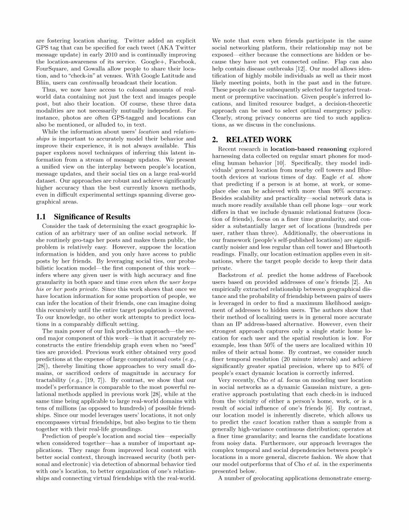
has three main components responsible for downloading Twit-ter data, visualization, and learning and inference. The datacollection component was described in the previous section.Figure 2 shows Flap’s visualization a sample of geo-activeusers in NYC. People are represented by pins on the mapand the red links denote friendships (either ground truth orinferred). Beyond standard Google Maps user interface el-ements, the visualization is controlled via the black toolbar4http://search.twitter.com/api/5http://www.census.gov/popest/metro/

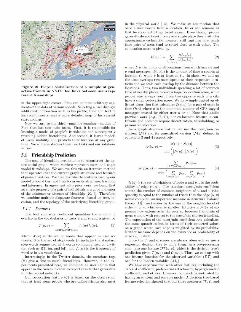
Figure 2: Flaps’s visualization of a sample of geo-active friends in NYC. Red links between users rep-resent friendships.

in the upper-right corner. Flap can animate arbitrary seg-ments of the data at various speeds. Selecting a user displaysadditional information such as his profile, time and text ofhis recent tweets, and a more detailed map of his currentsurroundings.

Now we turn to the third—machine learning—module ofFlap that has two main tasks. First, it is responsible forlearning a model of people’s friendships and subsequentlyrevealing hidden friendships. And second, it learns modelsof users’ mobility and predicts their location at any giventime. We will now discuss these two tasks and our solutionsin turn.

5.1 Friendship PredictionThe goal of friendship prediction is to reconstruct the en-

tire social graph, where vertices represent users and edgesmodel friendships. We achieve this via an iterative methodthat operates over the current graph structure and featuresof pairs of vertices. We first describe the features used by ourmodel of social ties, and then focus on its structure, learning,and inference. In agreement with prior work, we found thatno single property of a pair of individuals is a good indicatorof the existence or absence of friendship [20, 6]. Therefore,we combine multiple disparate features—based on text, lo-cation, and the topology of the underlying friendship graph.

5.1.1 FeaturesThe text similarity coefficient quantifies the amount of

overlap in the vocabularies of users u and v, and is given by

T (u, v) =∑

w∈W (u)∩W (v)\S

fu(w)fv(w), (1)

where W (u) is the set of words that appear in user u’stweets, S is the set of stop-words (it includes the standardstop words augmented with words commonly used on Twit-ter, such as RT, im, and lol), and fu(w) is the frequency ofword w in u’s vocabulary.

Interestingly, in the Twitter domain, the mentions tags(@) give a clue to user’s friendships. However, in the ex-periments presented here, we eliminate all user names thatappear in the tweets in order to report results that generalizeto other social networks.

Our co-location feature (C) is based on the observationthat at least some people who are online friends also meet

in the physical world [14]. We make an assumption thatonce a user tweets from a location, he or she remains atthat location until they tweet again. Even though peoplegenerally do not tweet from every single place they visit, thisapproximate co-location measure still captures how muchtime pairs of users tend to spend close to each other. Theco-location score is given by

C(u, v) =∑

`u,`v∈L

t(`u, `v)

d(`u, `v), (2)

where L is the union of all locations from which users u andv send messages, t(`u, `v) is the amount of time u spends atlocation `u while v is at location `v. In short, we add upthe time overlaps two users spend at their respective loca-tions and we scale each overlap by the distance between thelocations. Thus, two individuals spending a lot of commontime at nearby places receive a large co-location score, whilepeople who always tweet from two opposite ends of a cityhave a small co-location score. We have implemented an ef-ficient algorithm that calculates C(u, v) for a pair of users intime O(n) where n is the minimum number of GPS-taggedmessages created by either user u or v. Note that unlikeprevious work (e.g., [7, 1]), our co-location feature is con-tinuous and does not require discretization, thresholding, orparameter selection.

As a graph structure feature, we use the meet/min co-efficient (M) and its generalized version (ME) defined inequations 3 and 4 respectively.

M(u, v) =

∣∣N(u) ∩N(v)∣∣

min

(∣∣N(u)∣∣, ∣∣N(v)

∣∣) (3)

ME(u, v) =

∑n∈N(u)∩N(v)

pnupnv

min

( ∑n∈N(u)

pnu,∑

n∈N(v)

pnv

) (4)

N(u) is the set of neighbors of node u and pnu is the prob-ability of edge (n, u). The standard meet/min coefficientcounts the number of common neighbors of u and v (thisquantity is equal to the number of triads that the edge (u, v)would complete, an important measure in structural balancetheory [11]), and scales by the size of the neighborhood ofeither u or v, whichever is smaller. Intuitively, M(u, v) ex-presses how extensive is the overlap between friendlists ofusers u and v with respect to the size of the shorter friendlist.The expectation of the meet/min coefficient ME calculatesthe same quantities but in terms of their expected valueson a graph where each edge is weighted by its probability.Neither measure depends on the existence or probability ofedge (u, v) itself.

Since the T and C scores are always observed, we use aregression decision tree to unify them, in a pre-processingstep, into one feature DT (u, v), which is the decision tree’sprediction given T (u, v) and C(u, v). Thus, we end up withone feature function for the observed variables (DT ) andone for the hidden variables (ME).

We have experimented with other features, including theJaccard coefficient, preferential attachment, hypergeometriccoefficient, and others. However, our work is motivated byhaving an efficient and scalable model. A decision tree-basedfeature selection showed that our three measures (T , C, and

ME) jointly represent the largest information value. Finally,while calculating the features for all pairs of n users is anO(n2) operation, it can be significantly sped up via locality-sensitive hashing [8].

5.1.2 Learning and InferenceOur probabilistic model of the friendship network is a

Markov random field that has a hidden node for each possi-ble friendship. Since the friendship relationship is symmetricand irreflexive, our model contains n(n−1)/2 hidden nodes,where n is the number of users. Each hidden node is con-nected to an observed node (DT ) and to all other hiddennodes.

Ultimately, we are interested in the probability of exis-tence of an edge (friendship) given the current graph struc-ture and the pairwise features of the vertices (users) theedge is incident on. Applying Bayes’ theorem while assum-ing mutual independence of features DT and ME, we canwrite

P (E = 1|DT = d,ME = m) == P (DT = d|E = 1)P (ME = m|E = 1)P (E = 1)/Z= P (DT = d|E = 1)P (E = 1|ME = m)/Z

(5)where

Z =∑

i∈{0,1}

P (DT = d|E = i)P (E = i|ME = m).

E, DT , and ME are random variables that represent edgeexistence, DT score, and ME score, respectively. In equa-tion 5, we applied the equality

P (ME|E) = P (E|ME)P (E)/P (ME)

and subsequent simplifications so that we do not need toexplicitly model P (E).

At learning time, we first train a regression decision treeDT and prune it using ten-fold cross-validation to preventoverfitting. We also perform maximum likelihood learningof the parameters P (DT |E) and P (E|ME). We chose the de-cision tree pre-processing step for several reasons. First, thetext and location-based features considered individually orindependently have very poor predictive power. Therefore,models such as logistic regression tend to have low accu-racy. Furthermore, the relationships between the observedattributes of a pair of users and the their friendship is oftenquite complex. For example, it is not simply the case that afriendship is more and more likely to exist as people spendlarger and larger amounts of time near each other. Considertwo strangers that happen to take the same train to work,and tweet every time it goes through a station. Our datasetcontains a number of instances of this sort. During the trainride, their co-location could not be higher and yet they arenot friends on Twitter. This largely precludes success ofclassifiers that are looking for a simple decision surface.

At inference time, we use DT to make preliminary pre-dictions on the test data. Next, we execute a customizedloopy belief propagation algorithm that is initialized withthe probabilities estimated by DT (see Algorithm 1). Step 6is where an edge receives belief updates from the other edgesas well as the DT prior. Even though the graphical model isdense, our algorithm converges within several hundred iter-ations, due in part to the sufficiently accurate initializationand regularization provided by the decision tree. Note thatthe algorithm can also function in an online fashion: as new

ut

f1t fnt tdt wt. . .

ut+1

f1t+1 fnt+1 tdt+1 wt+1. . .

. . . . . .

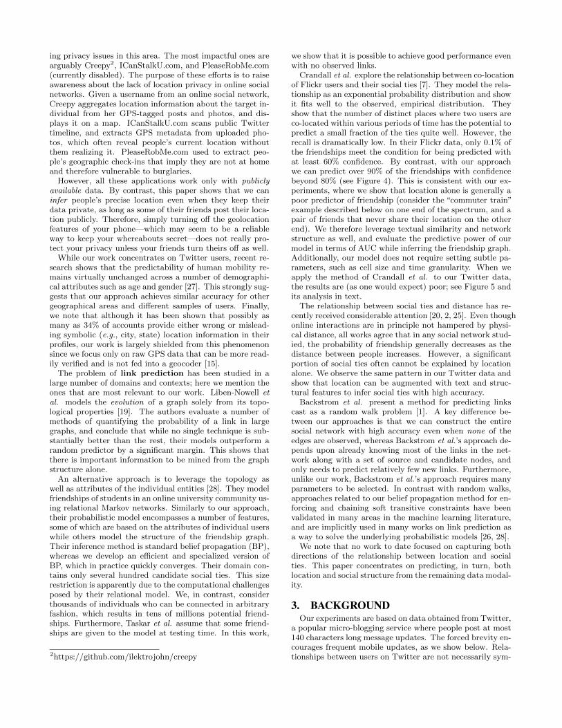
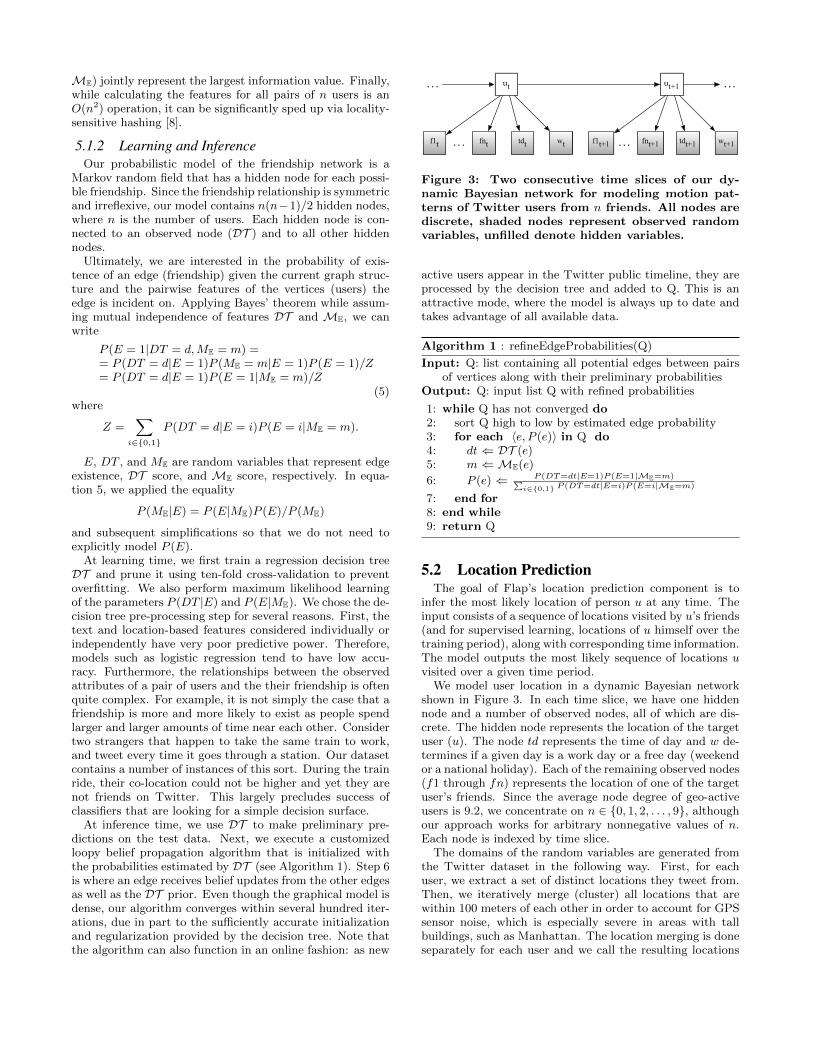
Figure 3: Two consecutive time slices of our dy-namic Bayesian network for modeling motion pat-terns of Twitter users from n friends. All nodes arediscrete, shaded nodes represent observed randomvariables, unfilled denote hidden variables.

active users appear in the Twitter public timeline, they areprocessed by the decision tree and added to Q. This is anattractive mode, where the model is always up to date andtakes advantage of all available data.

Algorithm 1 : refineEdgeProbabilities(Q)

Input: Q: list containing all potential edges between pairsof vertices along with their preliminary probabilities

Output: Q: input list Q with refined probabilities

1: while Q has not converged do2: sort Q high to low by estimated edge probability3: for each 〈e, P (e)〉 in Q do4: dt ⇐ DT (e)5: m ⇐ ME(e)

6: P (e) ⇐ P (DT=dt|E=1)P (E=1|ME=m)∑i∈{0,1} P (DT=dt|E=i)P (E=i|ME=m)

7: end for8: end while9: return Q

5.2 Location PredictionThe goal of Flap’s location prediction component is to

infer the most likely location of person u at any time. Theinput consists of a sequence of locations visited by u’s friends(and for supervised learning, locations of u himself over thetraining period), along with corresponding time information.The model outputs the most likely sequence of locations uvisited over a given time period.

We model user location in a dynamic Bayesian networkshown in Figure 3. In each time slice, we have one hiddennode and a number of observed nodes, all of which are dis-crete. The hidden node represents the location of the targetuser (u). The node td represents the time of day and w de-termines if a given day is a work day or a free day (weekendor a national holiday). Each of the remaining observed nodes(f1 through fn) represents the location of one of the targetuser’s friends. Since the average node degree of geo-activeusers is 9.2, we concentrate on n ∈ {0, 1, 2, . . . , 9}, althoughour approach works for arbitrary nonnegative values of n.Each node is indexed by time slice.

The domains of the random variables are generated fromthe Twitter dataset in the following way. First, for eachuser, we extract a set of distinct locations they tweet from.Then, we iteratively merge (cluster) all locations that arewithin 100 meters of each other in order to account for GPSsensor noise, which is especially severe in areas with tallbuildings, such as Manhattan. The location merging is doneseparately for each user and we call the resulting locations

unique. We subsequently remove all merged locations thatthe user visited fewer than five times and assign a uniquelabel to each remaining place. These labels are the domainsof u and fi’s. We call such places significant.

The above place indexing yields a total of 89,077 uniquelocations, out of which 25,830 were visited at least five timesby at least one user. There were 2,467,149 tweets totalposted from the significant locations in the 4 week modelevaluation period. Table 1 lists summary statistics.

We model each person’s location in 20 minute increments,since more than 90% of the users tweet with lower frequency.Therefore, the domain of the time of day random variabletd is {0, . . . , 71} (total of 24/0.3 time intervals in any givenday).

5.2.1 LearningWe explore both supervised and unsupervised learning of

user mobility. In the earlier case, for each user, we train aDBN on the first three weeks of data with known hiddenlocation values. In the latter case, the hidden labels areunknown to the system.

During supervised learning, we find a set of parameters(discrete probability distributions) θ that maximize the log-likelihood of the training data. This is achieved by optimiz-ing the following objective function.

θ? = argmaxθ

log(Pr(x1:t, y1:t|θ)

), (6)

where x1:t and y1:t represent the sequence of observed andhidden values, respectively, between times 1 and t, and θ?

is the set of optimal model parameters. In our implemen-tation, we represent probabilities and likelihoods with theirlog-counterparts to avoid arithmetic underflow.

For unsupervised learning, we perform expectation-maximi-zation (EM) [9]. In the E step, the values of the hiddennodes are inferred using the current DBN parameter values(initialized randomly). In the subsequent M step, the in-ferred values of the hidden nodes are in turn used to updatethe parameters. This process is repeated until convergence,at which point the EM algorithm outputs a maximum like-lihood point estimate of the DBN parameters. The corre-sponding optimization problem can be written as

θ? = argmaxθ

log∑y1:t

Pr(x1:t, y1:t|θ)

), (7)

where we sum over all possible values of hidden nodes y1:t.Since equation 7 is computationally intractable for sizabledomains, we simplify by optimizing its lower bound instead,similar to [13].

The random initialization of the EM procedure has a pro-found influence on the final set of learned parameter values.As a result, EM is prone to getting “stuck” in a local opti-mum. To mitigate this problem, we perform deterministicsimulated annealing [29]. The basic idea is to reduce theundesirable influence of the initial random set of parametersby “smoothing” the objective function so that it hopefullyhas fewer local optima. Mathematically, this is written as

θ?(τ1, . . . , τm) = argmaxθ

τi log∑y1:t

Pr(x1:t, y1:t|θ

) 1τi . (8)

Here, τ1, . . . , τm is a sequence of parameters, each of whichcorresponds to a different amount of smoothing of the origi-nal objective function (shown in equation 7). The sequence

is often called a temperature schedule in the simulated an-nealing literature, because equation 8 has analogs to freeenergy in physics. Therefore, we start with a relatively hightemperature τ1 and gradually lower it until τm = 1, whichrecovers the original objective function.

5.2.2 InferenceAt inference time, we are interested in the most likely ex-

planation of the observed data. That is, given a sequenceof locations visited by one’s friends, along with the corre-sponding time and day type, our model outputs the mostlikely sequence of locations one visited over the given timeperiod.

Flap runs a variant of Viterbi decoding to efficiently calcu-late the most likely state of the hidden nodes. In our model,Viterbi decoding is given by

y?1:t = argmaxy1:t

log(Pr(y1:t|x1:t)

), (9)

where Pr(y1:t|x1:t) is conditional probability of a sequence ofhidden states y1:t given a concrete sequence of observationsx1:t between times 1 and t.

In each time slice, we coalesce all observed nodes withtheir hidden parent node, and since we have one hiddennode in each time slice, we apply dynamic programming andachieve polynomial runtimes in a way similar to [17]. Specif-ically, the time complexity of our inference is O(T |Y |2),where T is the number of time slices and Y is the set ofpossible hidden state values (potential locations).

Therefore, the overall time complexity of learning and in-ference for any given target user is O(kT |Y |2), where k isthe number of EM iterations (k = 1 for supervised learning).This renders our model tractable even for very large domainsthat evolve over long periods of time with fine granularity.Next, we turn to our experiments, and analysis of results.

6. EVALUATIONFor clarity, we discuss experimental results for each of the

two Flap’s tasks separately.

6.1 Friendship PredictionWe evaluate Flap on friendship prediction using two-fold

cross-validation in which we train on LA and test on NYdata, and vice versa. We average the results over the tworuns. We varied the amount of randomly selected edgesprovided to the model at testing time from 0 to 50%.

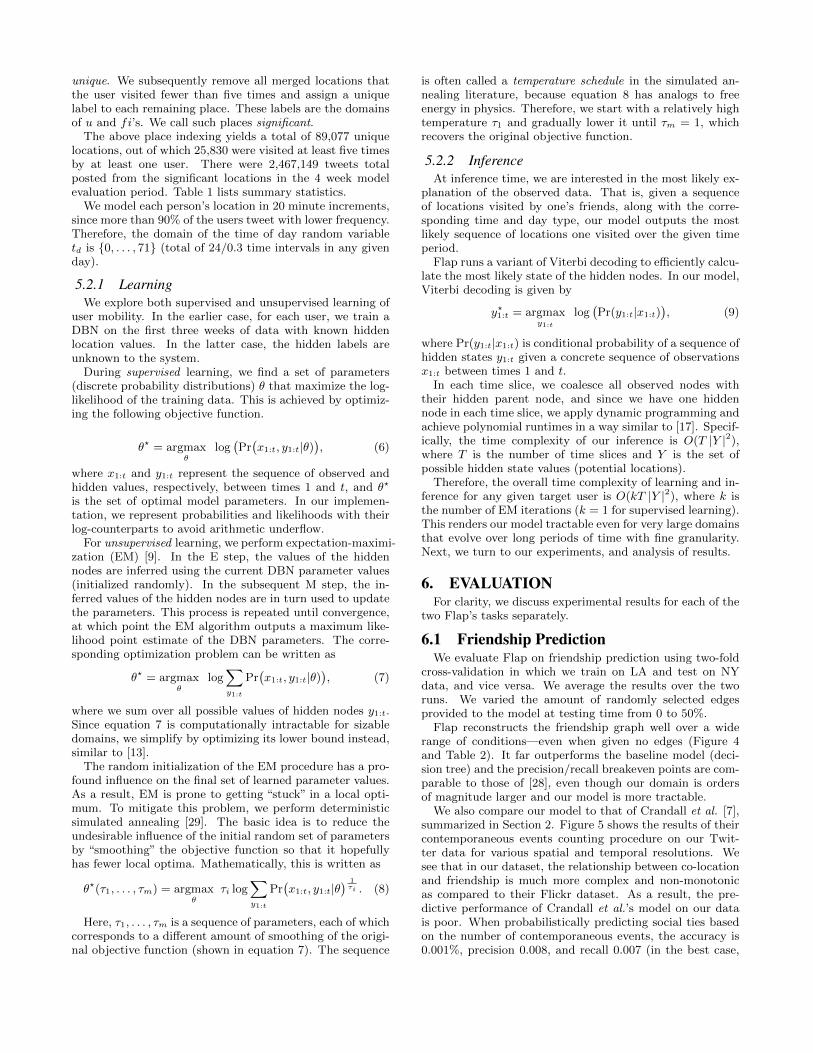
Flap reconstructs the friendship graph well over a widerange of conditions—even when given no edges (Figure 4and Table 2). It far outperforms the baseline model (deci-sion tree) and the precision/recall breakeven points are com-parable to those of [28], even though our domain is ordersof magnitude larger and our model is more tractable.

We also compare our model to that of Crandall et al. [7],summarized in Section 2. Figure 5 shows the results of theircontemporaneous events counting procedure on our Twit-ter data for various spatial and temporal resolutions. Wesee that in our dataset, the relationship between co-locationand friendship is much more complex and non-monotonicas compared to their Flickr dataset. As a result, the pre-dictive performance of Crandall et al.’s model on our datais poor. When probabilistically predicting social ties basedon the number of contemporaneous events, the accuracy is0.001%, precision 0.008, and recall 0.007 (in the best case,

0 0.1 0.2 0.3 0.4 0.5 0.6 0.7 0.8 0.9 10

0.1

0.2

0.3

0.4

0.5

0.6

0.7

0.8

0.9

1

False positive rate (1−Specificity)

True

pos

itive

rate

(Sen

sitiv

ity)

Random classifierCrandall et al.Dec. Tree Baseline0% observed edges10% observed edges25% observed edges50% observed edges

Figure 4: Averaged ROC curves for decision treebaseline, Crandall et al.’s model with the most fa-vorable setting of parameters (s = 0.001 and t = 4hours), and Flap.

#E 0% 10% 25% 50%

AUC Flap 6.5 × 107 0.78 0.82 0.88 0.95

AUC Crandall et al. 6.5 × 107 0.55 - - -

P=R Flap 6.5 × 107 0.28 0.36 0.47 0.64

P=R Crandall et al. 6.5 × 107 0.05 - - -

P=R Taskar et al. ∼ 4 × 102 N/A 0.47 0.58 0.73

Table 2: Summary of model evaluation. The #Ecolumn represents the number of candidate edgesthat exist in the social graph. The remainingcolumns denote the proportions of friendships givento the models at testing time. AUC is the area un-der the ROC curve; P=R denotes precision/recallbreakeven points. All results are based on our Twit-ter dataset, except for the P=R results for Taskaret al., which are based on their—much smaller—university dataset as their model does not scale tolarger networks; see text for details.

where s = 0.001 and t = 4 hours). There are two conclu-sions based on this result. First, similarly to Liben-Nowellet al. [20], we observe that geographic distance alone is notsufficient to accurately model social ties. And second, look-ing at the performance of [7]’s approach on the Flick datacomprising the entire world, versus its performance on ourLA and NYC data, we see that inferring relationships fromco-location data in dense and relatively small geographicalareas can be a more challenging task. This is important,as the majority of population lives and interacts in suchmetropolitan areas. However, our work shows that when weleverage additional information channels beyond co-location,and embed them in a probabilistic model, we can infer socialties quite well.

In order to explore how our model performs in the contextof strong ties, in both LA and NYC, we selected a subgraphthat contains only active users who are members of a cliqueof size at least eight. We again evaluated via cross-validationas above. Flap reconstructs the friendship network of the

0 5 10 15 20 25 30 350

0.1

0.2

0.3

0.4

0.5

0.6

0.7

0.8

0.9

1

Pr(fr

iend

ship

| #

of c

onte

mpo

rane

ous

even

ts =

n)

n

Twitter, s=0.001 t=1 dayTwitter, s=0.001 t=7 daysFlickr, s=0.001 t=1 dayFlickr, s=0.001 t=7 days

Figure 5: Comparison of the intensity of co-locationof pairs of users versus the probability of theirfriendship in our Twitter and Crandall et al.’s Flickrdatasets. We see that the relationship is more com-plex on Twitter, causing a simple model of socialties to achieve very low predictive accuracy. (s isthe size of cells in degrees in which we count theco-located events and t is the time slack; comparewith Figure 2 in [7].)

83 people with 0.92 precision and 0.85 recall, whereas thebaseline decision tree achieves precision of 0.83 and recallof 0.51. Interestingly, the co-location feature plays a majorrole here because the cliques of friends spend most of theirtime in relatively small areas.

6.2 Location PredictionOur evaluation is done in terms of accuracy—the percent-

age of timeslices for which the model infers the correct userlocation. We have a separate dynamic Bayesian networkmodel for each user.

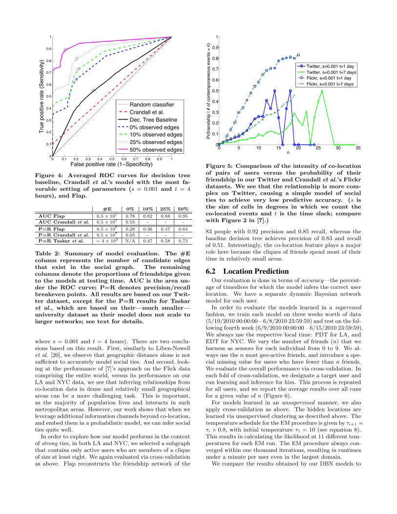
In order to evaluate the models learned in a supervisedfashion, we train each model on three weeks worth of data(5/19/2010 00:00:00 – 6/8/2010 23:59:59) and test on the fol-lowing fourth week (6/9/2010 00:00:00 – 6/15/2010 23:59:59).We always use the respective local time: PDT for LA, andEDT for NYC. We vary the number of friends (n) that weharness as sensors for each individual from 0 to 9. We al-ways use the n most geo-active friends, and introduce a spe-cial missing value for users who have fewer than n friends.We evaluate the overall performance via cross-validation. Ineach fold of cross-validation, we designate a target user andrun learning and inference for him. This process is repeatedfor all users, and we report the average results over all runsfor a given value of n (Figure 6).

For models learned in an unsupervised manner, we alsoapply cross-validation as above. The hidden locations arelearned via unsupervised clustering as described above. Thetemperature schedule for the EM procedure is given by τi+1 =τi × 0.8, with initial temperature τ1 = 10 (see equation 8).This results in calculating the likelihood at 11 different tem-peratures for each EM run. The EM procedure always con-verged within one thousand iterations, resulting in runtimesunder a minute per user even in the largest domain.

We compare the results obtained by our DBN models to

0 1 2 3 4 5 6 7 8 90

10

20

30

40

50

60

70

80

90

100

Number of Friends Leveraged (n)

Accu

racy

[%]

Supervised DBNUnsupervised DBNCho et al. PSMMNaiveRandom

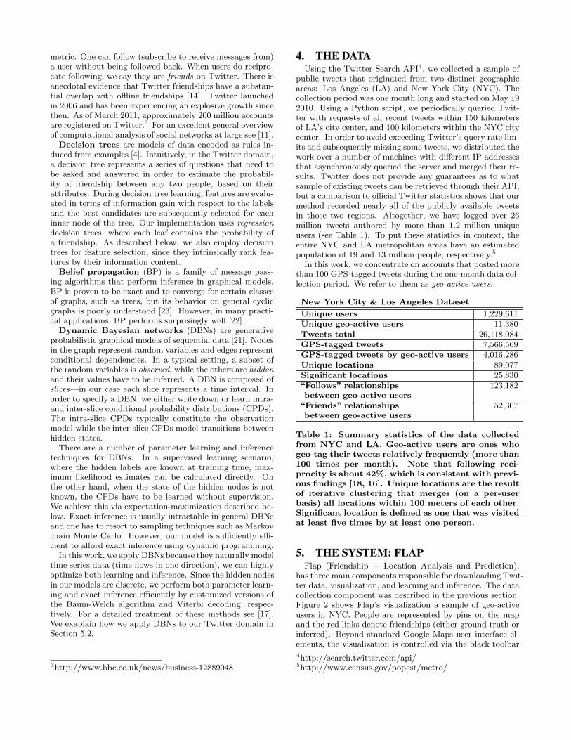
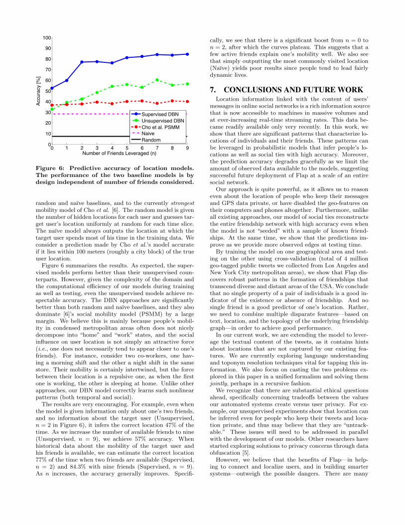
Figure 6: Predictive accuracy of location models.The performance of the two baseline models is bydesign independent of number of friends considered.

random and naıve baselines, and to the currently strongestmobility model of Cho et al. [6]. The random model is giventhe number of hidden locations for each user and guesses tar-get user’s location uniformly at random for each time slice.The naıve model always outputs the location at which thetarget user spends most of his time in the training data. Weconsider a prediction made by Cho et al.’s model accurateif it lies within 100 meters (roughly a city block) of the trueuser location.

Figure 6 summarizes the results. As expected, the super-vised models perform better than their unsupervised coun-terparts. However, given the complexity of the domain andthe computational efficiency of our models during trainingas well as testing, even the unsupervised models achieve re-spectable accuracy. The DBN approaches are significantlybetter than both random and naıve baselines, and they alsodominate [6]’s social mobility model (PSMM) by a largemargin. We believe this is mainly because people’s mobil-ity in condensed metropolitan areas often does not nicelydecompose into “home” and “work” states, and the socialinfluence on user location is not simply an attractive force(i.e., one does not necessarily tend to appear closer to one’sfriends). For instance, consider two co-workers, one hav-ing a morning shift and the other a night shift in the samestore. Their mobility is certainly intertwined, but the forcebetween their location is a repulsive one, as when the firstone is working, the other is sleeping at home. Unlike otherapproaches, our DBN model correctly learns such nonlinearpatterns (both temporal and social).

The results are very encouraging. For example, even whenthe model is given information only about one’s two friends,and no information about the target user (Unsupervised,n = 2 in Figure 6), it infers the correct location 47% of thetime. As we increase the number of available friends to nine(Unsupervised, n = 9), we achieve 57% accuracy. Whenhistorical data about the mobility of the target user andhis friends is available, we can estimate the correct location77% of the time when two friends are available (Supervised,n = 2) and 84.3% with nine friends (Supervised, n = 9).As n increases, the accuracy generally improves. Specifi-

cally, we see that there is a significant boost from n = 0 ton = 2, after which the curves plateau. This suggests that afew active friends explain one’s mobility well. We also seethat simply outputting the most commonly visited location(Naıve) yields poor results since people tend to lead fairlydynamic lives.

7. CONCLUSIONS AND FUTURE WORKLocation information linked with the content of users’

messages in online social networks is a rich information sourcethat is now accessible to machines in massive volumes andat ever-increasing real-time streaming rates. This data be-came readily available only very recently. In this work, weshow that there are significant patterns that characterize lo-cations of individuals and their friends. These patterns canbe leveraged in probabilistic models that infer people’s lo-cations as well as social ties with high accuracy. Moreover,the prediction accuracy degrades gracefully as we limit theamount of observed data available to the models, suggestingsuccessful future deployment of Flap at a scale of an entiresocial network.

Our approach is quite powerful, as it allows us to reasoneven about the location of people who keep their messagesand GPS data private, or have disabled the geo-features ontheir computers and phones altogether. Furthermore, unlikeall existing approaches, our model of social ties reconstructsthe entire friendship network with high accuracy even whenthe model is not “seeded” with a sample of known friend-ships. At the same time, we show that the predictions im-prove as we provide more observed edges at testing time.

By training the model on one geographical area and test-ing on the other using cross-validation (total of 4 milliongeo-tagged public tweets we collected from Los Angeles andNew York City metropolitan areas), we show that Flap dis-covers robust patterns in the formation of friendships thattranscend diverse and distant areas of the USA. We concludethat no single property of a pair of individuals is a good in-dicator of the existence or absence of friendship. And nosingle friend is a good predictor of one’s location. Rather,we need to combine multiple disparate features—based ontext, location, and the topology of the underlying friendshipgraph—in order to achieve good performance.

In our current work, we are extending the model to lever-age the textual content of the tweets, as it contains hintsabout locations that are not captured by our existing fea-tures. We are currently exploring language understandingand toponym resolution techniques vital for tapping this in-formation. We also focus on casting the two problems ex-plored in this paper in a unified formalism and solving themjointly, perhaps in a recursive fashion.

We recognize that there are substantial ethical questionsahead, specifically concerning tradeoffs between the valuesour automated systems create versus user privacy. For ex-ample, our unsupervised experiments show that location canbe inferred even for people who keep their tweets and loca-tion private, and thus may believe that they are “untrack-able.” These issues will need to be addressed in parallelwith the development of our models. Other researchers havestarted exploring solutions to privacy concerns through dataobfuscation [5].

However, we believe that the benefits of Flap—in help-ing to connect and localize users, and in building smartersystems—outweigh the possible dangers. There are many

exciting practical applications that have the potential tochange people’s lives that rely on location and link esti-mation. These include context-aware crowdsourcing, timelyand accurate recommendations, better local content, dis-ease prevention and containment, security, traffic modeling,emergency response, and others.

8. ACKNOWLEDGMENTSThis research was partly funded by ARO grant W911NF-

08-1- 0242, ONR grant N00014-11-10417, OSD grant W81XWH-08-C0740, and a gift from the Kodak Company. Theviews and conclusions contained in this document are thoseof the authors and should not be interpreted as necessarilyrepresenting the official policies, either expressed or implied,of any of these organizations.

9. REFERENCES[1] L. Backstrom and J. Leskovec. Supervised random

walks: predicting and recommending links in socialnetworks. In Proceedings of the fourth ACMinternational conference on Web search and datamining, pages 635–644. ACM, 2011.

[2] L. Backstrom, E. Sun, and C. Marlow. Find me if youcan: improving geographical prediction with socialand spatial proximity. In Proceedings of the 19thinternational conference on World wide web, pages61–70. ACM, 2010.

[3] R. Bell, Y. Koren, and C. Volinsky. Modelingrelationships at multiple scales to improve accuracy oflarge recommender systems. In KDD, pages 95–104,New York, NY, USA, 2007. ACM.

[4] L. Breiman et al. Classification and Regression Trees.Chapman & Hall, New York, 1984.

[5] A. B. Brush, J. Krumm, and J. Scott. Exploring enduser preferences for location obfuscation,location-based services, and the value of location. InUbicomp, Ubicomp ’10, pages 95–104, New York, NY,USA, 2010. ACM.

[6] E. Cho, S. A. Myers, and J. Leskovec. Friendship andmobility: User movement in location-based socialnetworks. ACM SIGKDD International Conference onKnowledge Discovery and Data Mining (KDD), 2011.

[7] D. Crandall, L. Backstrom, D. Cosley, S. Suri,D. Huttenlocher, and J. Kleinberg. Inferring social tiesfrom geographic coincidences. Proceedings of theNational Academy of Sciences, 107(52):22436, 2010.

[8] M. Datar, N. Immorlica, P. Indyk, and V. Mirrokni.Locality-sensitive hashing scheme based on p-stabledistributions. In Proceedings of the twentieth annualsymposium on Computational geometry, pages253–262. ACM, 2004.

[9] A. P. Dempster, N. M. Laird, and D. B. Rubin.Maximum likelihood from incomplete data via the emalgorithm. Journal of the Royal Statistical Society,39(1):1–38, 1977.

[10] N. Eagle and A. Pentland. Reality mining: sensingcomplex social systems. Personal and UbiquitousComputing, 10(4):255–268, 2006.

[11] D. Easley and J. Kleinberg. Networks, Crowds, andMarkets: Reasoning About a Highly Connected World.Cambridge University Press, 2010.

[12] S. Eubank, H. Guclu, V. Anil Kumar, M. Marathe,A. Srinivasan, Z. Toroczkai, and N. Wang. Modellingdisease outbreaks in realistic urban social networks.Nature, 429(6988):180–184, 2004.

[13] Z. Ghahramani. Learning dynamic Bayesian networks.In Adaptive Processing of Sequences and DataStructures, page 168. Springer, 1998.

[14] A. Gruzd, B. Wellman, and Y. Takhteyev. Imaginingtwitter as an imagined community. In AmericanBehavioral Scientist, Special issue on ImaginedCommunities, 2011.

[15] L. Hong, B. Suh, and E. H. Chi. Tweets from justinbieber’s heart: the dynamics of the “location” field inuser profiles. In ACM CHI, 2011.

[16] A. Java, X. Song, T. Finin, and B. Tseng. Why wetwitter: understanding microblogging usage andcommunities. In WebKDD/SNA-KDD, pages 56–65,New York, NY, USA, 2007. ACM.

[17] M. Jordan. Learning in graphical models. KluwerAcademic Publishers, 1998.

[18] H. Kwak, C. Lee, H. Park, and S. Moon. What isTwitter, a Social Network or a News Media? InWWW, April 2010.

[19] D. Liben-Nowell and J. Kleinberg. The link-predictionproblem for social networks. J. Am. Soc. Inf. Sci.Technol., 58:1019–1031, May 2007.

[20] D. Liben-Nowell, J. Novak, R. Kumar, P. Raghavan,and A. Tomkins. Geographic routing in socialnetworks. Proceedings of the National Academy ofSciences of the United States of America,102(33):11623, 2005.

[21] K. Murphy. Dynamic bayesian networks:representation, inference and learning. PhD thesis,University of California, Berkeley, 2002.

[22] K. P. Murphy, Y. Weiss, and M. I. Jordan. Loopybelief propagation for approximate inference: Anempirical study. In In Proceedings of Uncertainty inAI, pages 467–475, 1999.

[23] J. Pearl. Probabilistic Reasoning in IntelligentSystems: Networks of Plausible Inference. MorganKaufmann Publishers Inc., San Francisco, CA, USA,1988.

[24] A. S. Pentland. Honest Signals: How They Shape OurWorld. The MIT Press, 2008.

[25] S. Scellato, A. Noulas, R. Lambiotte, and C. Mascolo.Socio-spatial properties of online location-based socialnetworks. Proceedings of ICWSM, 11, 2011.

[26] D. Smith and J. Eisner. Dependency parsing by beliefpropagation. In Proceedings of the Conference onEmpirical Methods in Natural Language Processing,pages 145–156. Association for ComputationalLinguistics, 2008.

[27] C. Song, Z. Qu, N. Blumm, and A. Barabasi. Limits ofpredictability in human mobility. Science,327(5968):1018, 2010.

[28] B. Taskar, M.-F. Wong, P. Abbeel, and D. Koller.Link prediction in relational data. In in NeuralInformation Processing Systems, 2003.

[29] N. Ueda and R. Nakano. Deterministic annealing emalgorithm. Neural Networks, 11(2):271 – 282, 1998.