1

Title: Finding the sources of missing heritability in a yeast cross

Authors: Joshua S. Bloom1,2

, Ian M. Ehrenreich1,3

, Wesley Loo1,2

, Thúy-Lan Võ Lite1,2

,

Leonid Kruglyak1,4,5*

Affiliations: 1 Lewis-Sigler Institute for Integrative Genomics, Princeton University, Princeton, NJ

08540

2 Department of Molecular Biology, Princeton University, Princeton, NJ 08540

3 Molecular and Computational Biology Section, University of Southern California, Los

Angeles, CA 90089

4 Department of Ecology and Evolutionary Biology, Princeton University, Princeton, NJ

08540

5 Howard Hughes Medical Institute, Princeton University, Princeton, NJ 08540

*Correspondence should be addressed to L.K. (leonid@genomics.princeton.edu).

2

Abstract:

For many traits, including susceptibility to common diseases in humans, causal loci

uncovered by genetic mapping studies explain only a minority of the heritable

contribution to trait variation. Multiple explanations for this “missing heritability” have

been proposed. Here we use a large cross between two yeast strains to accurately estimate

different sources of heritable variation for 46 quantitative traits and to detect underlying

loci with high statistical power. We find that the detected loci explain nearly the entire

additive contribution to heritable variation for the traits studied. We also show that the

contribution to heritability of gene-gene interactions varies among traits, from near zero

to 50%. Detected two-locus interactions explain only a minority of this contribution.

These results substantially advance our understanding of the missing heritability problem

and have important implications for future studies of complex and quantitative traits.

One Sentence Summary: In yeast, detected loci explain the additive contribution of

genes to heritable variation in many quantitative traits.

3

Main Text:

Introduction

Individuals within species show heritable variation for many traits of biological and

medical interest. Most heritable traits follow complex inheritance patterns, with multiple

underlying genetic factors (1, 2). Finding these factors has been a central focus of modern

genetic research in humans, as well as in model organisms and agriculturally important

species (3-6). Recent work, most notably genome-wide association studies (GWAS) in

humans, has underscored the problem of “missing heritability”—although many genetic

loci have been identified for a wide range of traits, these typically explain only a minority

of the heritability of each trait, implying the existence of other, undiscovered genetic

factors (7).

Multiple non-mutually-exclusive explanations have been proposed for missing

heritability (7). One possibility is that the undiscovered factors could have effects that are

too small to be detected with current sample sizes, or even too small to ever be

individually detected with statistical significance (8-10). The existence of many small-

effect variants is supported by studies showing that a large proportion of heritable trait

variation is tagged when all GWAS markers are considered simultaneously (11, 12).

Because GWAS can only detect variants that are common in the population, another

possibility is that the undiscovered variants are too rare in the population to be captured

by GWAS (13). One recent proposal suggests that non-additive interactions among loci

(sometimes termed “epistasis”) inflate heritability measures, creating “phantom” rather

than missing heritability (14). Other proposed contributions to missing heritability

4

include inflated heritability estimates, structural variation, gene-environment interactions,

parent-of-origin effects, heritable epigenetic factors, and “entirely unforeseen sources” (7,

15). A better understanding of the sources of missing heritability is crucial for designing

studies to find the missing components.

We set out to investigate these questions in the yeast Saccharomyces cerevisiae.

We and others have previously used a cross between a lab strain and a wine strain to

investigate the genetic basis of many complex traits (16), including global gene

expression (17), protein abundance (18), telomere length (19), cell shape (20), gene

expression noise (21), and drug sensitivity (22), and we have demonstrated “missing

heritability” in this system (23). Recently, we used extreme quantitative trait locus (QTL)

mapping (X-QTL) a bulk segregant approach that uses pools of millions of cross progeny

(segregants), to detect many loci underlying heritable trait variation (24). We showed that

for one trait, loci detected by X-QTL explained most of the heritability. However, pooled

approaches do not allow direct estimates of heritability, the contribution of gene-gene

interactions or locus effect sizes. Here we use a large panel of individually genotyped and

phenotyped yeast segregants to accurately measure the heritable components of many

quantitative traits, discover the underlying loci, and examine the sources of missing

heritability.

Heritability and the role of gene-gene interactions

In order to estimate heritability and detect the underlying loci with high statistical power,

we constructed a panel of 1008 prototrophic haploid segregants from a cross between a

5

lab strain and a wine strain (Supplementary Fig. 1a,b and Supplementary Methods).

These strains differ by 0.5% at the sequence level (25). We sequenced the parent strains

to high coverage and compared the sequences to define 30,594 high-confidence single-

nucleotide polymorphisms (SNPs) that distinguish the strains and densely cover the

genome. We obtained comprehensive individual genotype information for each of 1008

segregants by highly multiplexed short-read sequencing (Supplementary Fig. 1c).

We sought to accurately measure a large number of quantitative traits in the

segregant panel. To do so, we implemented a high-throughput end-point colony size

assay and measured growth in multiple conditions, including different temperatures, pHs,

and carbon sources, as well as addition of metal ions and small molecules (16, 22, 24, 26)

(Supplementary Fig. 1d). We defined each trait as endpoint colony size normalized

relative to growth on control medium, (Supplementary Methods) and obtained

reproducible measurements with a strong heritable component for 46 traits

(Supplementary Table 1). Most of the traits were only weakly correlated with each other

(Supplementary Fig. 2).

Phenotypic variation in the segregant panel can be partitioned into the

contribution of heritable genetic factors (broad-sense heritability) and measurement

errors or other random environmental effects. Broad-sense heritability can in turn be

partitioned into the contribution of additive genetic factors (narrow-sense heritability),

dominance effects, gene-gene interactions, and gene-environment interactions (27, 28). In

our experiment, dominance effects are absent because the segregants are haploid, and

gene-environment interactions for a given trait should also be absent as all the segregants

6

are grown simultaneously under uniform conditions. Thus our estimates of broad-sense

heritability include additive and gene-gene interaction components, while our estimates

of narrow-sense heritability include only the additive component. The difference between

the two heritability measures (recently termed “phantom heritability” (14)) therefore

provides an estimate of the contribution of gene-gene interactions.

We estimated broad-sense heritability from repeatability of trait measurements

(Supplementary Methods). Estimating narrow-sense heritability usually involves

measuring phenotypic similarity for different degrees of relatedness. We took advantage

of a recently developed genomic approach in which narrow-sense heritability is estimated

by comparing phenotypic similarity among individuals with their actual genetic

relatedness, computed from dense genotype data (Supplementary Methods) (29). Among

the 46 traits, broad-sense heritability estimates ranged from 0.40 to 0.96, with a median

of 0.77. Narrow-sense heritability estimates ranged from 0.27 to 0.85, with a median of

0.55 (Fig. 1). We used the difference between these measures to estimate the fraction of

genetic variance due to gene-gene interactions, which ranged from 0.02 to 0.50 with a

median of 0.25. Thus, the genetic basis for variation in some traits is almost entirely due

to additive effects, while for others up to half of the heritable component is due to gene-

gene interactions.

Additive heritability explained by detected loci

Next, we sought to map the additive heritable variation to specific QTL. Simple linkage

analysis of one marker at a time revealed multiple QTL per trait (Supplementary

7

Methods). To more accurately capture the effects of each QTL while controlling for the

other QTL affecting the same trait, we used a step-wise forward-search approach to

detect QTL and build a multiple-regression model (Supplementary Methods). With this

approach, we detected a total of 591 QTL for 46 traits at an empirical false-discovery rate

(FDR) of 5%. We observed varying degrees of trait complexity, with a minimum of 5, a

maximum of 29, and a median of 12 QTL per trait. These numbers of QTL are

comparable to those previously seen for a smaller set of traits by X-QTL (24). Consistent

with theoretical predictions (30) and previous observations, we detected many more QTL

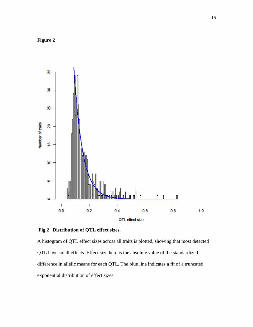
of small effect than of large effect (Fig. 2). Some traits showed a distribution of QTL

effect sizes roughly consistent with Orr‟s evolutionary model (30), whereas others

showed one or more larger-than-expected QTL (Supplementary Fig. 3).

Having identified QTL, we next measured the fraction of additive heritability

explained by our model of detected QTL for each trait. To obtain unbiased estimates, we

performed 10-fold cross-validation by detecting QTL in a subset of the segregant panel

and estimating the effects in the rest of the panel. Across the traits, the detected loci

explained between 72% and 100% of the narrow-sense heritability, with a median of 88%

(Fig. 3a). The detected loci explained between 41% and 84% of the broad-sense

heritability, with a median of 67%, and between 26% and 80% of the total phenotypic

variance, with a median of 49%. Thus, high statistical power provided by the large

segregant panel allowed us to detect QTL that jointly explain most of the additive

heritability for the traits studied here. By analyzing subsets of the data, we showed that

“missing” narrow-sense heritability can be explained by insufficient sample sizes (Fig.

8

3b). For instance, we detected 16 significant QTL, which jointly explain 78% of narrow-

sense heritability for growth in E6-berbamine, in a panel 1000 segregants, (Fig. 4a), but

only 2 of these, explaining 21% of narrow-sense heritability, also reached statistical

significance in a smaller panel of 100 segregants (Fig. 4b). For traits with mostly additive

genetics, the high fraction of variance explained by the detected QTL allowed us to

accurately predict individual trait values from QTL genotypes (Fig. 5).

Detecting two-locus interactions

Differences between the estimates of broad-sense and narrow-sense heritability for many

traits imply the presence of genetic interactions. We next sought to identify specific two-

locus interactions. For each trait, we first performed an exhaustive two-dimensional (2D)

scan for pairwise interactions. At a LOD score of 6.2, corresponding to an empirical FDR

of 10%, we detected significant QTL-QTL interactions for 17 of the 46 traits, with a total

of 23 interacting locus pairs. A 2D scan has low statistical power due to the large search

space. Power can be increased, at the cost of missing interactions between loci with no

main effects, by testing only for interactions between each locus with significant additive

effects and the rest of the genome (31). Using this approach, we detected interactions for

24 of the 46 traits, with a total of 78 QTL-QTL interactions at an FDR of 10%. We

observed a minimum of 1 and a maximum of 16 pairwise interactions per trait. These 78

pairs included 20 of the 23 locus pairs detected in the exhaustive 2D scan, suggesting that

two-locus interactions in which neither locus has a detectable main effect are uncommon.

For 47 of the 78 pairs, both loci were detected as significant in the single-locus search for

9

additive effects. In the remaining 31 cases, the additive effect of the second locus was too

small to reach genome-wide significance, although it was nominally significant in 10 of

these cases. These observations are broadly consistent with our previous work on genetic

interactions that affect gene expression traits (31, 32).

For most of the traits with a sizeable difference between broad-sense and narrow-

sense heritability, pairwise interactions were either not detected or explained little of the

difference (Fig. 6). The detected interaction effects were typically small (a median of

1.1% of genetic variance per interaction or a median of 3% of genetic variance per trait).

Only in a few cases did detected genetic interactions explain much of the difference

between broad-sense and narrow-sense heritability. Most notably, in the case of growth

on maltose, one strong interaction explained 14% of the genetic variance and 76% of the

difference between broad-sense and narrow-sense heritability (Fig. 6 inset).

Discussion

We have used a large panel of segregants from a cross between two yeast strains to

investigate the genetic architecture of 46 quantitative traits. We measured both the total

and the additive contributions of genetic factors to trait variation, and showed that these

often differ. The observed differences between total and additive heritability estimates

suggest that the contribution of genetic interactions to broad-sense heritability ranges

from zero to 50%. However, with a few exceptions, the specific combinations of loci that

account for these interactions remain elusive. There are several possible explanations for

this result. First, the statistical power to detect interactions is lower than the power to

10

detect main effects. Second, individual interaction effects are expected to be smaller than

additive effects, and hence their detection requires even larger sample sizes (14). Finally,

higher-order interactions among more than two loci could also contribute (33). Our

estimates of the contribution of interactions in a cross may overestimate their contribution

to trait heritability in a population, because a higher proportion of variance is expected to

be additive as allele frequencies depart from one-half (34).

The large size of the panel allowed us to detect specific loci that jointly account

for the great majority of the additive (narrow-sense) heritability of each trait (72-100%).

Human traits examined by GWAS vary in their genetic complexity (7), ranging from

macular degeneration, for which 5 variants in 3 genes explain roughly half of the genetic

risk (35), to height, for which 180 loci explain about 13% of heritability (36). However,

compared to our results in a yeast cross, GWAS typically detect a larger number of loci

explaining a smaller proportion of trait heritability. One obvious difference is that the

number of variants segregating in a cross between two strains is smaller than the number

of common variants segregating in a population sample. The difference is roughly a

factor of three for a neutral allele frequency spectrum, and potentially much larger if

functional variants are deleterious and hence shifted toward lower frequency

(Supplementary Methods). The human genome also offers a larger target size, perhaps by

a factor of five, for variants affecting a trait (Supplementary Methods). These very rough

estimates suggest that we might expect at least 15 times more loci to be found by GWAS

than the median of 12 loci per trait we observe in the yeast cross. Because of the

resolution of linkage analysis in our cross, some QTL may contain multiple linked

11

variants, further increasing the true number of loci. Several additional factors could lead

to a larger “missing heritability” in humans: the fraction of heritability due to genetic

interactions could be higher (14), rare variants may account for a disproportionately large

contribution of heritable variation (37-39), and some human traits might be inherently

more complex than yeast traits in that they integrate over physiological processes

involving a larger number of underlying gene pathways. Within-locus dominance effects

represent an additional source of genetic complexity in diploid organisms.

Our results are consistent with the suggestions that missing additive (narrow-

sense) heritability arises primarily from many loci with small but not infinitesimal

effects. These loci can be discovered in studies with sufficiently large sample sizes,

although the optimal study designs will depend on the population frequency spectra of

the causative alleles. Because all alleles are fixed at a frequency of one-half in a cross, we

cannot yet delineate the contributions of common and rare variants to inherited variation,

but we plan to do so in future studies.

References and notes

1. W. G. Hill, Philosophical Transactions of the Royal Society B: Biological

Sciences 365, 73 (January 12, 2010, 2010).

2. T. F. C. Mackay, E. A. Stone, J. F. Ayroles, Nat Rev Genet 10, 565 (2009).

3. E. S. Buckler et al., Science 325, 714 (August 7, 2009, 2009).

4. S. Atwell et al., Nature 465, 627 (2010).

5. T. F. Mackay et al., Nature 482, 173 (Feb 9, 2012).

6. D. L. Aylor et al., Genome Res 21, 1213 (Aug, 2011).

7. T. A. Manolio et al., Nature 461, 747 (Oct 8, 2009).

8. M. V. Rockman, Evolution 66, 1 (Jan, 2012).

9. M. A. Province, I. B. Borecki, Pac Symp Biocomput, 190 (2008).

10. D. B. Goldstein, N Engl J Med 360, 1696 (Apr 23, 2009).

11. J. Yang et al., Nat Genet 42, 565 (Jul, 2010).

12

12. P. M. Visscher, M. A. Brown, M. I. McCarthy, J. Yang, Am J Hum Genet 90, 7

(Jan 13, 2012).

13. J. K. Pritchard, Am J Hum Genet 69, 124 (Jul, 2001).

14. O. Zuk, E. Hechter, S. R. Sunyaev, E. S. Lander, Proc Natl Acad Sci U S A 109,

1193 (Jan 24, 2012).

15. E. E. Eichler et al., Nat Rev Genet 11, 446 (Jun, 2010).

16. I. M. Ehrenreich, J. P. Gerke, L. Kruglyak, Cold Spring Harb Symp Quant Biol

74, 145 (2009).

17. R. B. Brem, G. Yvert, R. Clinton, L. Kruglyak, Science 296, 752 (Apr 26, 2002).

18. E. J. Foss et al., Nat Genet 39, 1369 (Nov, 2007).

19. T. Gatbonton et al., PLoS Genet 2, e35 (Mar, 2006).

20. J. Ansel et al., PLoS Genet 4, e1000049 (Apr, 2008).

21. S. Nogami, Y. Ohya, G. Yvert, PLoS Genet 3, e31 (Feb 23, 2007).

22. E. O. Perlstein et al., Chem Biol 13, 319 (Mar, 2006).

23. R. B. Brem, L. Kruglyak, Proc Natl Acad Sci U S A 102, 1572 (Feb 1, 2005).

24. I. M. Ehrenreich et al., Nature 464, 1039 (Apr 15, 2010).

25. D. M. Ruderfer, S. C. Pratt, H. S. Seidel, L. Kruglyak, Nat Genet 38, 1077 (Sep,

2006).

26. M. Hampsey, Yeast 13, 1099 (Sep 30, 1997).

27. D. S. Falconer, T. F. C. Mackay, Introduction to quantitative genetics.

(Longman, Essex, England, ed. 4th, 1996), pp. xiii, 464 p.

28. M. Lynch, B. Walsh, Genetics and analysis of quantitative traits. (Sinauer,

Sunderland, Mass., 1998), pp. xvi, 980 p.

29. P. M. Visscher et al., PLoS Genet 2, e41 (Mar, 2006).

30. H. A. Orr, Evolution 54, 13 (Feb, 2000).

31. J. D. Storey, J. M. Akey, L. Kruglyak, PLoS Biol 3, e267 (Aug, 2005).

32. R. B. Brem, J. D. Storey, J. Whittle, L. Kruglyak, Nature 436, 701 (Aug 4, 2005).

33. R. D. Dowell et al., Science 328, 469 (Apr 23, 2010).

34. W. G. Hill, M. E. Goddard, P. M. Visscher, PLoS Genet 4, e1000008 (Feb, 2008).

35. J. Maller et al., Nat Genet 38, 1055 (Sep, 2006).

36. H. Lango Allen et al., Nature 467, 832 (Oct 14, 2010).

37. J. A. Tennessen et al., Science, (May 21, 2012).

38. A. Keinan, A. G. Clark, Science 336, 740 (May 11, 2012).

39. M. R. Nelson et al., Science, (May 17, 2012).

40. D. C. Amberg, D. Burke, J. N. Strathern, Cold Spring Harbor Laboratory.,

Methods in yeast genetics : a Cold Spring Harbor Laboratory course manual.

(Cold Spring Harbor Laboratory Press, Cold Spring Harbor, N.Y., ed. 2005,

2005), pp. xvii, 230 p.

41. R Development Core Team. (R Foundation for Statistical Computing, Vienna,

Austria, 2012).

42. H. Li, R. Durbin, Bioinformatics 25, 1754 (Jul 15, 2009).

43. H. Li et al., Bioinformatics 25, 2078 (Aug 15, 2009).

44. K. W. Broman, H. Wu, S. Sen, G. A. Churchill, Bioinformatics 19, 889 (May 1,

2003).

13

45. M. D. Abramoff, Magalhaes, P.J., Ram, S.J., Biophotonics International 11, 36

(2004).

46. G. Pau, F. Fuchs, O. Sklyar, M. Boutros, W. Huber, Bioinformatics 26, 979 (Apr

1, 2010).

47. C. Loader. (2012).

48. M. M. Douglas Bates, Ben Bolker. (2011).

49. S. H. Lee, N. R. Wray, M. E. Goddard, P. M. Visscher, Am J Hum Genet 88, 294

(Mar 11, 2011).

50. J. B. Endelman, Plant Genome 4, 250 (2011).

51. L. Chen, J. D. Storey, Genetics 173, 2371 (Aug, 2006).

52. R. W. Doerge, G. A. Churchill, Genetics 142, 285 (Jan, 1996).

53. L. Kruglyak, D. A. Nickerson, Nat Genet 27, 234 (Mar, 2001).

54. E. Birney et al., Nature 447, 799 (Jun 14, 2007).

Supplementary Materials

Materials and Methods

Figs. S1, S2, S3

References (40-54)

Table S1, S2

Acknowledgements:

We thank David Botstein, Megan McClean, Erik Andersen, Frank Albert, Sebastian

Treusch, Rajarashi Ghosh, and Xin Wang for comments on the manuscript, Yue Jia for

technical assistance, and Eric Lander for discussions. This work was supported by NIH

grant R37 MH59520, a James S. McDonnell Centennial Fellowship, and the Howard

Hughes Medical Institute (L.K.), an NSF fellowship (J.S.B.), NIH postdoctoral

fellowship F32 HG51762 (I.M.E.), and NIH grant P50 GM071508 to the Center for

Quantitative Biology at the Lewis-Sigler Institute of Princeton University.

14

Figure 1

Fig.1 | Heritability for 46 yeast traits.

The broad-sense heritability (H2) for each trait (Y-axis) is plotted against the narrow-

sense heritability (h2; X-axis). Error bars show standard errors in heritability estimates.

The diagonal line represents H2 = h

2 and is shown as a visual guide.

15

Figure 2

Fig.2 | Distribution of QTL effect sizes.

A histogram of QTL effect sizes across all traits is plotted, showing that most detected

QTL have small effects. Effect size here is the absolute value of the standardized

difference in allelic means for each QTL. The blue line indicates a fit of a truncated

exponential distribution of effect sizes.

16

Figure 3

A B

Fig.3 | Most additive heritability is explained by detected QTL.

(A) The narrow-sense heritability (h2) for each trait (Y-axis) is plotted against the total

variance explained by detected QTL (X-axis). Error bars show standard errors. The

diagonal line represents h2 = (variance explained by detected QTL) and is shown as a

visual guide. (B) The average fraction of additive genetic variance explained (Y-axis) is

plotted against number of segregants used for QTL detection (X-axis). Error bars show

standard errors.

17

Figure 4

A

B

Figure 4 | QTL detection for a complex trait.

LOD score (log10 of the odds ratio for linkage) is plotted against the genetic map. Red

stars indicate statistically significant QTL. (A) LOD score plot with 1005 segregants for

growth in E6-berbamine. (B) LOD score plot with 100 segregants for growth in E6-

berbamine. The 15 significant QTL in A explain 78% of the narrow-sense heritability,

compared with 21% for the 2 significant QTL in B.

18

Figure 5

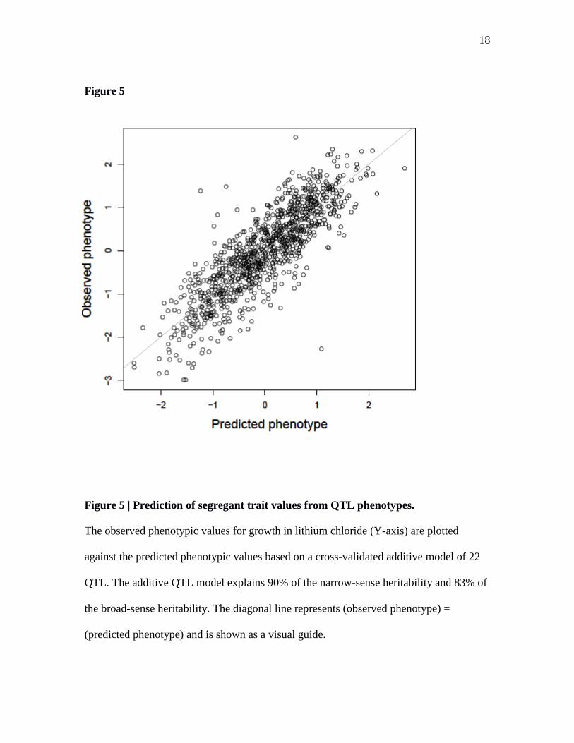
Figure 5 | Prediction of segregant trait values from QTL phenotypes.

The observed phenotypic values for growth in lithium chloride (Y-axis) are plotted

against the predicted phenotypic values based on a cross-validated additive model of 22

QTL. The additive QTL model explains 90% of the narrow-sense heritability and 83% of

the broad-sense heritability. The diagonal line represents (observed phenotype) =

(predicted phenotype) and is shown as a visual guide.

19

Figure 6

Figure 6 | Non-additive variance explained by QTL-QTL interactions.

A histogram of the fraction of non-additive variance explained by detected QTL-QTL

interactions per trait is plotted. (Inset) Phenotypes for growth in maltose are shown,

grouped by two-locus genotypes at the two interacting QTL on chromosomes VII and XI.

This QTL-QTL interaction explained 76% of the difference between broad-sense and

narrow-sense heritability.

20

Supplementary Materials:

Materials and methods:

Construction of segregant panel

We crossed a prototrophic BY parent (derived from a cross of BY4716 and BY4700) that

is MATa with a prototrophic RM parent (derived from RM11-1a) that is MAT

ho∆::HphMX4 flo8∆::NatMX4 AMN1-BY. Diploid zygotes were recovered and

sporulated for 5-7 days in SPO++ sporulation medium

(http://dunham.gs.washington.edu/sporulationdissection.htm)

in a roller drum at room temperature. Tetrads were dissected (40) using the MSM 400

dissection microscope (Singer Instrument Company Ltd.). Colonies from four-spore

tetrads were innoculated into 150 μL of YNB + 2% glucose in 96 well plates (Corning;

07-200-656), grown for 48 hours at 30° without shaking, and stored as frozen stocks in

20% glycerol. 1056 four-spore tetrads that displayed 2:2 segregation of hygromycin

resistance, G418 resistance, and mating type were retained. A Biomek FX (Beckman

Coulter) was used to select one segregant from each four-spore tetrad for downstream

analysis.

Power calculations

We calculated statistical power (1- β) for sample sizes of 100 and 1000 segregants in R

using the „power.t.test‟ function (41). Power was calculated over a range of effect sizes,

where effect size was calculated as the percent genetic variance explained by a single

QTL. To correct for multiple testing over thousands of markers across the genome, a

genome-wide significance threshold (α) of p < 2*10-4

was used.

DNA preparation and sequencing library construction

21

Segregants were innoculated into 1 mL deep-well 96-well plates (Thermo Scientific; 12-

565-395) in 800 μL of YPD and grown 2 days at 30° without shaking. Plates were sealed

with Breathe-Easy gas-permeable membranes (Sigma-Aldrich; Z380059). DNA was

extracted using 96-well DNEasy Blood & Tissue kits (Qiagen; 69582). DNA

concentrations were determined using the Quant-it dsDNA high sensitivity DNA

quantification kit (Invitrogen; Q-33120) and the Biotek Synergy 2 plate reader. DNA was

diluted to 1.66 ng/μL. Per sample, 15 μL of 1.66 ng/μL DNA was added to 4 μl of 5X

Nextera HMW buffer, 0.95 μl of water, and 0.05 μl of Nextera Enzyme Mix (Epicentre;

GA0911-96). The transposition reaction was performed for 5 minutes at 55°. 100 μl of

water was added to each sample, and the samples were purified using the MinElute kit

(Qiagen; 28053). 15 μl of the purified fragmented DNA was PCR-amplified and

barcoded with custom 5 bp sequences using ExTaq polymerase (Takara, RR001A) and

between 15 and 30 PCR cycles. 5 μl of each PCR-amplified sample was combined into

one 96-plex library. The combined library was loaded on a 2% agarose gel, and the 350

bp to 650 bp region was excised and gel-extracted using QiaQuick Gel Extraction Kit

(Qiagen; 28704). Final libraries were diluted to 3.3 ng/μl and sequenced using the single-

end module on a HiSeq 2000 (Illumina) with 100 bp reads.

Determining segregant genotypes

Custom R and python code was used to demultiplex the sequencing data and trim ends.

Sequencing reads were assigned to segregants based on the 5 base-pair (bp) barcode at

the beginning of each read. The internal 19 bp transposon sequence and 10 bp on the

right end of each read were removed. Reads were aligned to the S288C reference genome

using the Burrows-Wheeler Aligner (BWA) (42) with the '-q 30' parameter.

SAMTools(43) was run with the „view‟ command and „-bHsq 1' parameters to retain

uniquely mapping reads. Sequence variants were identified using SAMTools (43) with

the „mpileup' command and parameters '-d 10000 -D -u'. 42,689 high-confidence

22

sequence variants between BY and RM were determined from sequencing the parental

strains at greater than 50-fold coverage. Variants in the segregants were restricted to these

42,689 expected sites using 'bcftools view' (43) with the parameters '-N -c -g -v -P flat'.

Genotype likelihoods for the BY and RM alleles for each genotypic variant were

extracted from the VCF file using custom R code.

For each segregant and chromosome, a hidden Markov model (HMM) was used to

calculate the posterior likelihood that the read data was coming from the BY allele, the

RM allele, a BY gene-conversion event or an RM gene-conversion event. Genotypes

were called as the BY variant if the log10 ratio of the BY posterior likelihood and the RM

posterior likelihood was greater than 2, the RM variant if this ratio was less than -2, and

missing data if between -2 and 2. 1,008 out of 1,056 segregants had between 25 and 120

recombination breakpoints and at least 35,000 markers with genotype calls, and these

were retained for downstream analysis. Genotypic markers were excluded if their allele

frequency was greater than 56% or less than 45%, or if they were not called in 99% of the

segregants. This resulted in a final set of 30,594 genotypic markers. Markers with

missing data were imputed using the Viterbi algorithm as implemented in the R/qtl

package (44). Adjacent markers with the same genotypes in all segregants were collapsed

to one unique marker, resulting in a final set of 11,623 unique genotypic markers.

Phenotyping by end-point growth on agar plates

Individual segregants were inoculated in at least 2 different plate configurations into 384-

well plates (Themo Scientific; 264574) with 50 mL of YPD and grown for 36 to 48 hours

in a 30° degree incubator without shaking. Each target agar plate was made with 50 mL

of media (YPD or YNB) and with drug or condition of choice (Supplementary Table 1).

The Singer Rotor HDA pinning robot was used to pin the segregants to the agar plates.

Before pinning, each 384-well plate was mixed for 1 minute at 2000 RPM using a

MixMate (Eppendorf). Segregants were pinned to the agar plates with 100% pin pressure

23

and 384 long pins (Singer Instruments; RP-MP-3L). After pinning, the plates were

incubated at 30°, or the specified condition temperature (Supplementary Table 1), for

approximately 48 hours. Plates were scanned face-up and without lids on an Epson 700

transparency scanner with 400 dpi resolution and a greyscale bit-depth of 8. Images were

saved as TIFFs or 99% quality JPEGs. The pixel coordinates of the centers of the four

corner colonies for each plate were manually identified using ImageJ (45).

Custom R code was written to determine the size of each colony. Expected colony

positions were calculated using manually identified coordinates of the corner colonies for

each plate. Images were segmented using k-means clustering on the distribution of pixel

intensities across a plate. The Voronoi region of each 9-pixel diameter circular seed,

corresponding to the expected location of a colony, was used together with the segmented

image to match colonies to their expected positions. This was implemented using

functions in the EBImage (46) R package. The radius of each colony was calculated as

pixel _ count. Colonies with more than 15 pixels touching the edge of the image and

colonies larger than 3,500 pixels were removed and treated as missing data in

downstream analysis. Irregular colonies, representing image processing or pinning

artifacts, were removed if perimeter

2 * pixel _ count1 and radius>20. These irregular colonies

were also treated as missing data for downstream analysis. Colonies on each edge of a

plate were tested for difference with all other colonies on the plate using a Wilcoxon

rank-sum test. All colonies on an edge with p<0.05 were treated as missing data and

excluded from downstream analysis. Images were further inspected manually, and

colonies subject to pinning or image-processing artifacts were removed. To normalize for

occasional subtle within-plate spatial growth artifacts, a robust locally weighted

regression was fit to the radius measurements using functions in the locfit R package

(47). The residuals were used for downstream analysis. End-point growth measurements

were normalized for growth on control media by fitting a regression for effect of growth

on control media and using the residuals for downstream analysis. 140 conditions were

24

assayed. If multiple doses of a compound were tested, the dose with the highest

heritability and phenotype data for at least 600 segregants was retained. Traits with

narrow-sense heritability less than 25% were excluded from downstream analysis.

Calculating heritability

Broad-sense heritability was calculated using replicated segregant data and a random

effects ANOVA. This was implemented using the „lmer‟ function in the lme4 R package

(48). The variance components 2

G, the genetic variance due to effect of segregant, and

2

E, the error variance, were calculated, and broad sense-heritability was estimated as

22

2

EG

G . Standard errors were calculated by delete-one jackknife.

Narrow-sense heritability was calculated for each trait using a linear mixed model (49).

This can be written as y=β1N+Zu+e. Here y is a vector of phenotype values for N

segregants, β is the overall mean, and 1N is a vector of N ones. Z is an NxN identity

matrix, u is a vector of random effects (BLUPs or breeding values for each segregant),

and e is a vector of residuals. The variance structure of the phenotypes is written as

V=AσA2 + IσEV

2 , where A is the relatedness matrix between all pairs of segregants,

estimated from our genotype data as the proportion of markers shared IBD between all

pair of segregants, I is an NxN identity matrix, σA2 is the polygenic additive genetic

variance explained by the SNPs, and σEV2 is the error variance. Variance components

were estimated using the rrBLUP R package (50), and narrow-sense heritability was

estimated as 22

2

EVA

A . Standard errors were calculated by delete-one jackknife.

Although the average genetic relatedness among the segregants is 0.5, it varies due to

random Mendelian segregation, and the actual relatedness for any pair of segregants can

25

be calculated from high-density genotype data as the proportion of SNP alleles shared by

these segregants. In our segregant panel, the standard deviation of relatedness was 0.048.

Mapping additive QTL

46 traits were chosen for QTL mapping based on the criteria described above. Each trait

was scaled to have mean 0 and variance 1. We tested for linkage by calculating LOD

scores for each genotypic marker and each trait as n (ln( 1 R2) / 2 ln( 10 )) , where R is the

Pearson correlation coefficient between the segregant genotypes at the marker and

segregant trait values (28).

To estimate significance empirically, assignment of phenotype to each segregant was

randomly permuted 1000 times while maintaining the correlation structure among

phenotypes. The maximum LOD score for each chromosome and trait was retained (51).

The FDR was calculated as the ratio of expected peaks to observed peaks across different

LOD thresholds. Genetic markers corresponding to QTL peaks which were significant at

an FDR of 5% were added to a linear model for each trait. Trait-specific linear models

that included the significant QTL genotypes as additive covariates were computed, and

phenotypic residuals were estimated. Phenotypic residuals for each trait were then used

for another round of QTL detection (52). This process of peak detection, calculation of

empirical significance thresholds, and expansion of the linear model for each trait to

include significant QTLs detected at each step was repeated 4 times. The LOD thresholds

corresponding to a 5% FDR at each step were 2.68, 2.92, 3.72 and 4.9.

Calculating effect size and variance explained by additive QTL

For each trait, a multiple regression linear model was computed with trait-specific QTL

genotypes as independent variables. Phenotypes for each trait were scaled to have mean 0

and variance 1. The multiple regression coefficients are the standardized differences in

26

allelic means for each QTL while controlling for the effects of other segregating QTL.

The square of the multiple regression coefficient is the fraction of phenotypic variance

explained by a QTL. The fitted truncated exponential distribution in Figure 2 is

parameterized as bx

rblbe

ee

bnw, where x is the absolute value of the multiple regression

coefficient pooled across traits and QTL, n is the number of bins, w is the bin size, l and r

are left and right truncation points and b is estimated using maximum likelihood. Here

l=0.12 and r=0.35 to correspond to the magnitude of effect sizes where power is nearly

100% and to exclude large-effect QTL.

The total phenotypic variance explained by the multiple regression QTL model is the R2

from the model, which was calculated using the „fitqtl‟ function in R/qtl. Unbiased

estimates of the total phenotypic variance explained by the multiple QTL model were

calculated by standard 10-fold cross validation. The segregants were randomly split into

10 equal-sized groups, 9 groups were combined for QTL detection using the algorithm

described above, and the remaining group was used to estimate QTL effect sizes. This

process was repeated for each of the 10 groups, and the average of the 10 estimates was

calculated.

Detecting QTL-QTL interactions

For computational efficiency, the marker set was reduced to 4,420 by picking one

physical marker closest to each centimorgan (cm) position on the genetic map. For the

full genome scan for interacting QTL, a LOD score corresponding to the likelihood ratio

of a model that includes an interaction term, y=ax+bz+cxz+d, to a model that does not,

y=ax+bz+d, was computed for each trait and every marker pair. Here, y is the residuals

vector for each trait after fitting the additive QTL model, x is the genotype vector at one

position in the genome, z is the genotype vector at another position in the genome at least

25 cm away from x, and a,b,c, and d are estimated parameters specific to each trait and

marker pair (31, 32). FDR at different LOD thresholds was calculated by dividing the

27

average number of peaks obtained in 1000 permutations of the data that scramble the

segregant identities by the number of peaks observed in the real data.

To increase statistical power, we tested for interactions between each locus with

significant additive effects and the rest of the genome. A LOD score for interaction was

computed in exactly the same manner as for the full 2D scan described above, except that

x was constrained to genotypes corresponding to trait-specific significant additive QTL.

FDR was calculated as above.

Conversion factors for yeast vs. human expected numbers of QTL

The number of variants segregating in a cross between two strains is smaller than the

number of (common) variants segregating in a population sample. If the causal variants

follow a neutral allele frequency spectrum, then under the standard neutral model of

population genetics, the relationship between the number of variants segregating in a

cross of two haploid strains (S2) and the number of common variants segregating in a

population (Sf) with minor allele frequency f is Sf = S2ln )1

(f

f(ref. (53)). By setting

f to 0.05, we obtain a ratio Sf/S2 of approximately three (2.94). The ratio is 2.2 for f = 0.1

and 4.6 for f = 0.01. If the functional variants are at least weakly deleterious, and hence

skewed toward lower frequency, the conversion factors will be larger.

Several approaches can be used to obtain a rough idea of relative target size for mutation.

The yeast genome is 12 Mb, whereas the coding regions of the human genome alone are

~30 Mb, and at least the same amount of non-coding sequence is expected to be

functional based on selective constraint (54). If we assume that the number of loci

involved in a trait is proportional to the number of bases available for mutations with

functional consequences, human traits should be more complex than yeast traits by

28

roughly a factor of 5. Similarly, yeast has ~5700 genes compared to ~20,000 for humans,

which gives a conversion factor of ~3.5.

29

Supplementary Figures:

Figure S1.

The design of the segregant panel is shown in (A). (B) Curves illustrating statistical

power are shown for mapping populations of 100 (blue) and 1000 (red) segregants at a

genome-wide significance threshold. (C) An image of endpoint colony growth is shown

for 384 segregants, with the outlines of colonies, as detected by our image processing

software, indicated in red. (D) Parental genotype likelihood ratios are plotted (Y-axis)

against genome position (X-axis) for a representative segregant; the red bars indicate

parental haplotype calls, and the vertical blue bars delineate chromosomes.

30

Figure S2.

The Spearman correlation coefficients for all pairs of traits are shown. Numbers in table

cells indicate (100 * correlation coefficient).

31

Figure S3.

For each trait, the effect sizes of detected QTL are sorted from largest to smallest, and the

cumulative phenotypic variance explained is plotted (Y-axis) against the number of

detected QTL (X-axis). Under Orr‟s model, the curves should extrapolate to the origin;

deviations from this expectation imply the presence of large-effect QTL for the

corresponding traits.

32

Supplementary Tables:

Table S1. Drug doses, heritability statistics, and QTL summary statistics for traits

investigated in this study.

Table S2. Table of detected QTL. Positions, effect sizes, confidence intervals and genes

underneath detected QTL for each trait are listed.

Author Contributions:

Experiments were designed by J.S.B., I.M.E., and L.K. Experiments were performed by

J.S.B., I.M.E., W.L., and T.L. Analyses were conducted by J.S.B. The manuscript was

written by J.S.B. and L.K. and incorporates comments by all other authors.