finding the most interesting patterns in a database ...€¦ · finding the most interesting...

Journal of Machine Learning Research 3 (2002) 833-862 Submitted 12/01; Published 12/02

Finding the Most Interesting Patterns in a DatabaseQuickly by Using Sequential Sampling

Tobias Scheffer [email protected]

University of Magdeburg, FIN/IWSP.O. Box 4120, 39016 Magdeburg, Germany

Stefan Wrobel [email protected]

FhG AiS, Schloß Birlinghoven 53754 Sankt Augustin, GermanyUniversity of Bonn, Informatik III, Romerstr. 164, 53117 Bonn, Germany

Editors: Carla E. Brodley and Andrea Danyluk

Abstract

Many discovery problems,e.g.,subgroup or association rule discovery, can naturally be cast asn-best hypotheses problems where the goal is to find then hypotheses from a given hypothesis spacethat score best according to a certain utility function. We present a sampling algorithm that solvesthis problem by issuing a small number of database queries while guaranteeing precise bounds onthe confidence and quality of solutions. Known sampling approaches have treated single hypothesisselection problems, assuming that the utility is the average (over the examples) of some function— which is not the case for many frequently used utility functions. We show that our algorithmworks for all utilities that can be estimated with bounded error. We provide these error boundsand resulting worst-case sample bounds for some of the most frequently used utilities, and provethat there is no sampling algorithm for a popular class of utility functions that cannot be estimatedwith bounded error. The algorithm is sequential in the sense that it starts to return (or discard)hypotheses that already seem to be particularly good (or bad) after a few examples. Thus, thealgorithm is almost always faster than its worst-case bounds.

Keywords: Sampling, online learning, incremental learning, large databases.

1. Introduction

The general task of knowledge discovery in databases (KDD) is the “automatic extraction of novel,useful, and valid knowledge from large sets of data” (Fayyad et al., 1996). An important aspectof this task is thescalability, i.e., the ability to successfully perform discovery in ever-growingdatasets. Unfortunately, even with discovery algorithms optimized for very large datasets, for manyapplication problems it is infeasible to process all of the given data. Whenever more data is availablethan can be processed in reasonable time, an obvious strategy is to use only a randomly drawnsampleof the data. Clearly, if some part of the data is not looked at, it is impossible in generalto guarantee that the results produced by the discovery algorithm will be identical to the resultsreturned on the complete dataset. If the use of sampled datasets is to be more than a practitioner’s“hack”, sampling must be combined with discovery algorithms in a fashion that allows us to givethe userguaranteesabout how much the results obtained using sampling differ from the optimal(non-sampling based) results. The goal of a sampling discovery algorithm then is to guarantee thisquality using the minimum amount of examples (Toivonen, 1996).

c©2002 Tobias Scheffer and Stefan Wrobel.

SCHEFFER ANDWROBEL

Known algorithms that do give rigorous guarantees on the quality of the returned solutions forall possible problems usually require an impractically large amount of data. One approach to findingpractical algorithms is to process a fixed amount of data but determine the possible strength of thequality guarantee dynamically, based on characteristics of the data; this is the idea of self-boundinglearning algorithms (Freund, 1998) and shell decomposition bounds (Haussler et al., 1996, Langfordand McAllester, 2000). Another approach (which we pursue) is to demand a certain fixed qualityand determine the required sample size dynamically based on characteristics of the data that havealready been seen; this idea has originally been referred to as sequential analysis (Dodge and Romig,1929, Wald, 1947, Ghosh et al., 1997).

In the machine learning context, the idea of sequential sampling has been developed into the Ho-effding race algorithm (Maron and Moore, 1994) which processes examples incrementally, updatesthe empirical utility values simultaneously, and starts to output (or discard) hypotheses as soonas it becomes very likely that some hypothesis is near-optimal (or very poor, respectively). Theincremental greedy learning algorithm PALO (Greiner, 1996) has been reported to require manytimes fewer examples than the worst-case bounds suggest. In the context of knowledge discovery indatabases, too, sequential sampling algorithms can reduces the required amount of data significantly(Haas and Swami, 1992, Domingo et al., 1999).

These existing sampling algorithms address discovery problems where the goal is to select froma space of possible hypothesesH one of the elements with the maximal value of aninstance-averagingquality function f , or all elements with anf -value above a user-given threshold (e.g.,all association rules with sufficient support). With instance-averaging quality functions, the qualityof a hypothesish is the average across all instances in a datasetD of an instance quality functionfinst.

Many discovery problems, however, cannot easily be cast in this framework. Firstly, it is oftenmore natural for a user to ask for then best solutions instead of the single best or all hypothesesabove a threshold – see,e.g.,Wrobel (1997). Secondly, many popular quality measures cannot beexpressed as an averaging quality function. This is the casee.g., for all functions that combinegenerality and distributional properties of a hypothesis; generally, both generality and distributionalproperties (such as accuracy) have to be considered for association rule and subgroup discoveryproblems. The task of subgroup discovery (Kl¨osgen, 1995) is to find maximally general subsets ofdatabase transactions within which the distribution of a focused feature differs maximally from thedefault probability of that feature in the whole database. As an example, consider the problem offinding groups of customers who are particularly likely (or unlikely) to buy a certain product.

In this paper, we present a general sampling algorithm for then-best hypotheses problem thatworks for any utility functions that can be estimated with bounded error. To this end, in Section 2,we first define then-best hypotheses problem more precisely and identify appropriate quality guar-antees. Section 3 then presents the generic sequential sampling algorithm. In Section 4, we provethat many of the popular utility functions that have been used in the area of knowledge discovery indatabases indeed can be estimated with bounded error, giving detailed bounds. In order to motivatethe instantiations of our sampling algorithm and put it into context, we first define some relevantknowledge discovery tasks in Section 4. For one popular class of functions that cannot be used byour algorithm, we prove that there cannot be a sampling algorithm at all. Our results thus also givean indication as to which of the large numbers of popular utility functions are preferable with respectto sampling. In Section 6, we evaluate our results and discuss their relation to previous work.

834

FINDING PATTERNS IN A DATABASE BY USING SEQUENTIAL SAMPLING

2. Approximating n-Best Hypotheses Problems

In many cases, it is more natural for a user to ask for then best solutions instead of the single bestor all hypotheses above a threshold. Suchn-best hypotheses problems can be stated more preciselyas follows – adapted from Wrobel (1997), where that formulation is used for subgroup discovery:

Definition 1 (n-best hypotheses problem)Let D be a database of instances, H a set of possiblehypotheses, f: H×D→ IR≥0 a quality or utility function on H, and n,1≤ n < |H|, the number ofdesired solutions. The n-best hypotheses problemis to find a set G⊆ H of size n such that

there is no h′ ∈H: h′ 6∈G and f(h′,D) > fmin, where fmin := minh∈G f (h,D).

Whenever we use sampling, the above optimality property cannot be guaranteed, so we must findappropriate alternative guarantees. Since forn-best problems, the exact quality and rank of hy-potheses are often not central to the user, it is sufficient to guarantee thatG indeed “approximately”contains then best hypotheses. We can operationalize this by guaranteeing that, with high probabil-ity, there will be no non-returned hypothesis that is “significantly” better than the worst hypothesisin our solution. More precisely, we will use the following problem formulated along the lines ofPAC (probably approximately correct) learning:

Definition 2 (Approximate n-best hypotheses problem)Let D, H, f and n as in the precedingdefinition. Then letδ, 0 < δ ≤ 1, be a user-specified confidence, andε ∈ IR+ a user-specifiedmaximal error. Theapproximaten-best hypotheses problemis to find a set G⊆H of size n such that

with confidence1−δ, there is no h′ ∈H: h′ 6∈G and f(h′,D) > fmin+ε, where fmin :=minh∈G f (h,D).

In other words, we want to find a set ofn hypotheses such that, with high confidence, no otherhypothesis outperforms any one of them by more thanε, where f is an arbitrary performance mea-sure.

In order to design an algorithm for this problem, we need to make certain assumptions about thequality function f . Ideally, an algorithm should be capable of working (at least) with the kinds ofquality functions that have already proven themselves useful in practical applications. If the problemis to classifydatabase items (i.e., to find a total function mapping database items to class labels),accuracyis often used as the utility criterion. For the discovery ofassociation rules, by contrast,one usually relies ongeneralityas the primary utility criterion (Agrawal et al., 1993). Finally, forsubgroup discovery, it is commonplace to combine both generality anddistributional unusualness,resulting in relatively complex evaluation functions – see,e.g.,Klosgen (1996) for an overview.

In light of the large range of existing and possible future utility functions and in order to avoidunduly restricting our algorithm, we will not make syntactic assumptions aboutf . In particular,unlike Domingo et al. (1999), we will not assume thatf is a single probability nor that it is (a func-tion of) an average of instance properties. Instead, we only assume that it is possible to determinea confidence interval fthat bounds the possible difference between the true utility (on the wholedatabase) and estimated utility (on the sample) with a certain confidence. We expect the confidenceinterval to narrow as the sample size grows. As we will show in Section 4 below, finding such con-fidence intervals is straightforward for classification accuracy, and is also possible for all but oneof the popular utility functions from association rule and subgroup discovery. More precisely, wedefine a confidence interval forf as follows.

835

SCHEFFER ANDWROBEL

Definition 3 (Utility confidence interval) Let f be a utility function, let h∈H be a hypothesis. Letf (h,D) denote the true quality of h on the entire dataset,f (h,Qm) its estimated quality computedbased on a sample Qm⊆ D of size m. Then E: IN× IR→ IR is a utility confidence boundfor f ifffor anyδ, 0 < δ≤ 1,

PrS[| f (h,Qm)− f (h,D)| ≤ E(m,δ)]≥ 1−δ (1)

Equation 1 says thatE(m,δ) provides a two-sided confidence interval onf (h,Qm) with con-fidenceδ. In other words, the probability of drawing a sampleQm (when drawingm transactionsindependently and identically distributed fromD), such that the difference between true and esti-mated utility of any hypothesis disagree byE(m,δ) or more (in either direction) lies belowδ. If, inaddition, for anyδ,0 < δ ≤ 1 and anyε there is a numberm such thatE(m,δ) ≤ ε we say that theconfidence intervalvanishes. In this case, we can shrink the confidence interval (at any confidencelevel δ) to arbitrarily low nonzero values by using a sufficiently large sample. We sometimes writethe confidence interval for a specific hypothesish asEh(m,δ). Thus, we allow the confidence inter-val to depend on characteristics ofh, such as the variance of one or more random variables that theutility of h depends on.

We will discuss confidence intervals for different functions of interest in Section 4. Here, as asimple example, let us only note that iff is simply a probability over the examples, then we can usethe Chernoff inequality to derive a confidence interval; whenf is the average (over the examples)of some function with a bounded range, then the Hoeffding inequality implies a confidence interval.Of course, we should also note that the trivial functionE(m,δ) := Λ is an error probability boundfunction for anyf with lower bound of zero and upper bound ofΛ, but we will see that we can onlyguarantee termination when the confidence interval vanishes as the sample size grows.

3. The GSS Sampling Algorithm

A general approach to designing a sampling algorithm is to use an appropriate error probabilitybound to determine the required number of examples for a desired level of confidence and accu-racy. When estimating a single probability, Chernoff bounds (Chernoff, 1952) that are used in PACtheory (Kearns and Vazirani, 1994, Wolpert, 1995, Vapnik, 1996) and many other areas of statis-tics and computer science can be used to determine appropriate sample bounds (Toivonen, 1996).When such algorithms are implemented, the Chernoff bounds can be replaced by tighter normal ort distribution tables.

Unfortunately, the straightforward extension of such approaches to selection or comparisonproblems like then-best hypotheses problem leads to unreasonably large bounds: to avoid errors inthe worst case, we have to take very large samples to recognize small differences in utility, even ifthe actual differences between hypotheses to be compared are very large. This problem is addressedby sequentialsampling methods (Dodge and Romig, 1929, Wald, 1947) which have also been re-ferred to asadaptivesampling methods (Domingo et al., 1998). The idea of sequential sampling isthat when the difference between two frequencies is very large after only a few examples, then wecan conclude that one of the probabilities is greater than the other with high confidence; we neednot wait for the sample size specified by the Chernoff bound, which we have to wait for when thefrequencies are similar. Sequential sampling methods have been reported to reduce the requiredsample size by several orders of magnitude –e.g.,Greiner and Isukapalli (1996).

In our algorithm (Table 1), we combine sequential sampling with the popular “loop reversal”technique found in many KDD algorithms. Instead of processing hypotheses one after another,

836


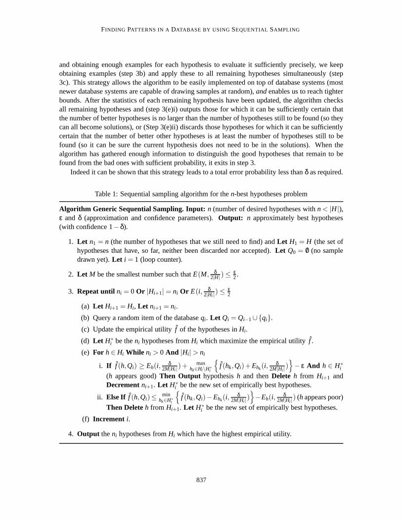
and obtaining enough examples for each hypothesis to evaluate it sufficiently precisely, we keepobtaining examples (step 3b) and apply these to all remaining hypotheses simultaneously (step3c). This strategy allows the algorithm to be easily implemented on top of database systems (mostnewer database systems are capable of drawing samples at random),andenables us to reach tighterbounds. After the statistics of each remaining hypothesis have been updated, the algorithm checksall remaining hypotheses and (step 3(e)i) outputs those for which it can be sufficiently certain thatthe number of better hypotheses is no larger than the number of hypotheses still to be found (so theycan all become solutions), or (Step 3(e)ii) discards those hypotheses for which it can be sufficientlycertain that the number of better other hypotheses is at least the number of hypotheses still to befound (so it can be sure the current hypothesis does not need to be in the solutions). When thealgorithm has gathered enough information to distinguish the good hypotheses that remain to befound from the bad ones with sufficient probability, it exits in step 3.

Indeed it can be shown that this strategy leads to a total error probability less thanδ as required.

Table 1: Sequential sampling algorithm for then-best hypotheses problem

Algorithm Generic Sequential Sampling. Input: n (number of desired hypotheses withn< |H|),ε and δ (approximation and confidence parameters).Output: n approximately best hypotheses(with confidence 1−δ).

1. Let n1 = n (the number of hypotheses that we still need to find) andLet H1 = H (the set ofhypotheses that have, so far, neither been discarded nor accepted).Let Q0 = /0 (no sampledrawn yet).Let i = 1 (loop counter).

2. Let M be the smallest number such thatE(M, δ2|H| )≤ ε

2.

3. Repeat until ni = 0 Or |Hi+1|= ni Or E(i, δ2|Hi |)≤ ε

2

(a) Let Hi+1 = Hi, Let ni+1 = ni .

(b) Query a random item of the databaseqi . Let Qi = Qi−1∪{qi}.(c) Update the empirical utilityf of the hypotheses inHi.

(d) Let H∗i be theni hypotheses fromHi which maximize the empirical utilityf .

(e) For h∈Hi While ni > 0 And |Hi|> ni

i. If f (h,Qi) ≥ Eh(i, δ2M|Hi |) + max

hk∈Hi\H∗i

{f (hk,Qi)+Ehk(i,

δ2M|Hi |)

}− ε And h ∈ H∗

i

(h appears good)Then Output hypothesish and thenDelete h from Hi+1 andDecrementni+1. Let H∗

i be the new set of empirically best hypotheses.

ii. Else If f (h,Qi)≤ minhk∈H∗

i

{f (hk,Qi)−Ehk(i,

δ2M|Hi |)

}−Eh(i, δ

2M|Hi |) (happears poor)

Then Deleteh from Hi+1. Let H∗i be the new set of empirically best hypotheses.

(f) Increment i.

4. Output theni hypotheses fromHi which have the highest empirical utility.

837

SCHEFFER ANDWROBEL

Theorem 4 When the algorithm terminates, it will output a group G of exactly n hypotheses suchthat, with confidence1− δ, no other hypothesis in H has a utility that is more thanε higher thanthe utility of any hypothesis that has been returned:

Pr[∃h∈ H \G : f (h) > fmin+ ε]≤ δ (2)

where fmin = minh′∈G{ f (h′)}; assuming that|H| ≥ n.

The proof of Theorem 4 can be found in Appendix A

Theorem 5 (Termination) If for any δ (0 < δ ≤ 1) and ε > 0 there is a number m such thatE(m,δ)≤ ε, then the algorithm can be guaranteed to terminate.

The correctness of Theorem 5 follows immediately from Step 3e of the algorithm. Theorem 5says that we can guarantee termination if the confidence interval vanishes for large numbers ofexamples. This is a benign assumption that is satisfied by most utility functions, as we will see inthe next section.

4. Instantiations

In order to implement the algorithm for a given utility function we have to find a utility confidenceinterval E(m,δ) that satisfies Equation 1 for that specificf . In this section, we will introducesome terminology, and present a list of confidence intervals for the utility functions that are mostcommonly used in knowledge discovery systems. Since the database is constant, we abbreviatef (h,D) as f (h) throughout this section.

Most of the known utility functions refer toconfidence, accuracy, “statistical unusualness”,supportor generalityof hypotheses. Let us quickly put these terms into perspective. Associationrules and classification rules are predictive; forsomedatabase transactions they predict the valueof an attribute given the values of some other attributes. For instance, the rule “beer= 1→ chips=1” predicts that a customer transaction with attribute beer= 1 will also likely have the attributechips= 1. However, when a customer does not buy beer, then the rule does not make any prediction.In particular, the rule does not imply that a customer who does not buy beer does not buy chipseither. The number of transactions in the database for which the rule makes a correct prediction (inour example, the number of transactions that include beer and chips) is called thesupport, or thegenerality.

Among those transitions for which the rule does make a prediction, some predictions may beerroneous. Theconfidenceis the fraction of correct predictions among those transactions for whicha prediction is made. Theaccuracy, too, quantifies the probability of a hypothesis conjecturing acorrect attribute. However, the term accuracy is typically used in the context of classification andrefers to the probability of a correct classification for a future transaction whereas the confidencerefers to the database used for training. From a sampling point of view, confidence and accuracycan be treated equally. In both cases, a relative frequency is measured on a small sample; fromthis frequency we want to derive claims on the underlying probability. It does not make a differencewhether this probability is itself a frequency on a much larger instance space (confidence) or a “real”probability (accuracy), defined with respect to an underlying distribution on instances.

Subgroups are of a more descriptive character. They describe that the value of an attributediffers from the global mean value within a particular subgroup of transactions without actually

838


conjecturing the value of that attribute for a new transaction. Thegeneralityof a subgroup is thefraction of all transactions in the database that belong to that subgroup. The termstatistical unusu-alnessrefers to the difference between the probabilityp0 of an attribute in the whole database andthe probabilityp of that attribute within the subgroup. Usually, subgroups are desired to be bothgeneral (largeg) and statistically unusual (large|p0− p|). There are many possible utility functionsfor subgroup discovery which trade generality against unusualness (Kl¨osgen, 1996). Unfortunately,none of these functions can be expressed as the average (over all transactions) of an instance utilityfunction. But, in Sections 4.2 through 4.4 we will show how instantiations of the GSS algorithmcan solve sampling problems for these functions.

We would like to conclude this subsection with a remark on whether a sample should be drawnwith or without replacement. When the utility function is defined with respect to a finite database, itis, in principle, possible to draw the sample without replacement. When the sample size reaches thedatabase size, we can be certain to have solved the real, not just the approximate,n best hypothesisproblem. So it should be possible to give a tighter utility confidence bound when the sample isdrawn without replacement. Consider the simple case when the utility is a probability. When thesample is drawn with replacement, the relative frequency corresponding to the target probability isgoverned by the binomial distribution whereas, when the sample is drawn without replacement, it isgoverned by the hyper-geometrical distribution for which we can specify a tighter bound. However,for sample sizes in the order of magnitude that we envision, the only feasible way of calculating boththe hyper-geometrical distribution and the binomial distribution is to use a normal approximation.But the normal approximation of both distributions are equal and so we cannot realize the smalladvantage that drawing without replacement seems to promise. The same situation arises with otherutility functions.

4.1 Instance-Averaging Functions

This simplest form of a utility function is the average, over all example instances, of some instanceutility function finst(h,qi) whereqi ∈D. The utility is then defined asf (h) = 1

|D| ∑|D|i=1 finst(h,qi) (the

average over the whole database) and the estimated utility isf (h,Qm) = 1m ∑qi∈Qm

finst(h,qi) (aver-age over the example queries). An easy example of an instance-averaging utility is classificationaccuracy (wherefinst(h,qi) is 0 or 1). Besides being useful by itself, this class of utility functionsserves as an introductory example of how confidence intervals can be derived. We assume that thepossible range of utility values lies between 0 andΛ. In the case of classification accuracy,Λ equalsone.

We can use theHoeffding inequality (Hoeffding, 1963) to bound the chance that an arbitrary(bounded) random variableX takes a value that is far away from its expected valueE(X) (Equation3). WhenX is a relative frequency andE(X) the corresponding probability, then we know thatΛ = 1. This special case of the Hoeffding inequality is calledChernoff ’sinequality.

Pr[|X−E(X)| ≤ ε]≥ 1−2exp

{−2m

ε2

Λ2

}(3)

We now need to define a confidence interval that satisfies Equation 1, where the Hoeffding inequalityserves as a tool to prove Equation 1. We can easily see that Equation 4 satisfies this condition.

E(m,δ) =

√Λ2

2mlog

2δ

(4)

839

SCHEFFER ANDWROBEL

In Equation 5 we insert Equation 4 into Equation 1. We apply the Hoeffding inequality (Equation3) in Equation 6 and obtain the desired result in Equation 7.

Pr[| f (h,Qm)− f (h)|> E(m,δ)

]= Pr

[| f (h,Qm)− f (h)|>

√Λ2

2mlog

2δ

](5)

≤ 2exp

−2m

(√Λ2

2m log 2δ

)2

Λ2

(6)

≤ 2exp

{− log

2δ

}= δ (7)

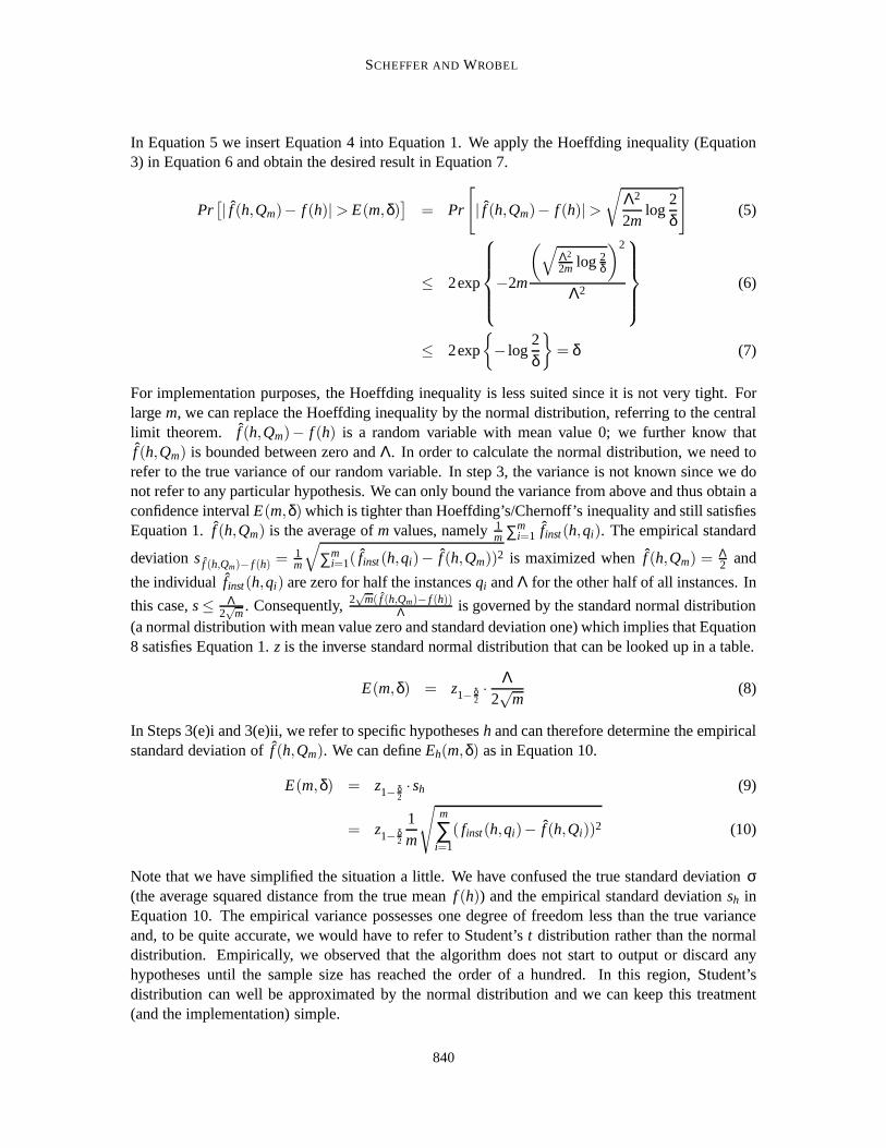
For implementation purposes, the Hoeffding inequality is less suited since it is not very tight. Forlargem, we can replace the Hoeffding inequality by the normal distribution, referring to the centrallimit theorem. f (h,Qm)− f (h) is a random variable with mean value 0; we further know thatf (h,Qm) is bounded between zero andΛ. In order to calculate the normal distribution, we need torefer to the true variance of our random variable. In step 3, the variance is not known since we donot refer to any particular hypothesis. We can only bound the variance from above and thus obtain aconfidence intervalE(m,δ) which is tighter than Hoeffding’s/Chernoff’s inequality and still satisfiesEquation 1. f (h,Qm) is the average ofm values, namely1

m ∑mi=1 finst(h,qi). The empirical standard

deviationsf (h,Qm)− f (h) = 1m

√∑m

i=1( finst(h,qi)− f (h,Qm))2 is maximized whenf (h,Qm) = Λ2 and

the individual finst(h,qi) are zero for half the instancesqi andΛ for the other half of all instances. In

this case,s≤ Λ2√

m. Consequently,2√

m( f (h,Qm)− f (h))Λ is governed by the standard normal distribution

(a normal distribution with mean value zero and standard deviation one) which implies that Equation8 satisfies Equation 1.z is the inverse standard normal distribution that can be looked up in a table.

E(m,δ) = z1− δ2· Λ2√

m(8)

In Steps 3(e)i and 3(e)ii, we refer to specific hypothesesh and can therefore determine the empiricalstandard deviation off (h,Qm). We can defineEh(m,δ) as in Equation 10.

E(m,δ) = z1− δ2·sh (9)

= z1− δ2

1m

√m

∑i=1

( finst(h,qi)− f (h,Qi))2 (10)

Note that we have simplified the situation a little. We have confused the true standard deviationσ(the average squared distance from the true meanf (h)) and the empirical standard deviationsh inEquation 10. The empirical variance possesses one degree of freedom less than the true varianceand, to be quite accurate, we would have to refer to Student’st distribution rather than the normaldistribution. Empirically, we observed that the algorithm does not start to output or discard anyhypotheses until the sample size has reached the order of a hundred. In this region, Student’sdistribution can well be approximated by the normal distribution and we can keep this treatment(and the implementation) simple.

840


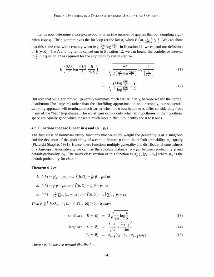
Let us now determine a worst-case bound onm (the number of queries that our sampling algo-

rithm issues). The algorithm exits the for loop (at the latest) whenE(

m, δ2|H|)≤ ε

2. We can show

that this is the case with certainty whenm≥ 2Λ2

ε2 log 4|H|δ . In Equation 11, we expand our definition

of E(m,δ). TheΛ and log-terms cancel out in Equation 12; we can bound the confidence intervalto ε

2 in Equation 12 as required for the algorithm to exit in step 3e.

E

(2Λ2

ε2 log4|H|

δ,

δ2|H|

)=

√√√√ Λ2

2(

2Λ2

ε2 log 4|H|δ

) log2(δ

2|H|) (11)

=

√√√√ε2

4

log 4|H|δ

log 4|H|δ

=ε2

(12)

But note that our algorithm will generally terminate much earlier; firstly, because we use the normaldistribution (for largem) rather than the Hoeffding approximation and, secondly, our sequentialsampling approach will terminate much earlier when then best hypotheses differ considerably frommany of the “bad” hypotheses. The worst case occurs only when all hypotheses in the hypothesisspace are equally good which makes it much more difficult to identify then best ones.

4.2 Functions that are Linear in g and (p− p0)

The first class of nontrivial utility functions that we study weight the generalityg of a subgroupand the deviation of the probability of a certain featurep from the default probabilityp0 equally(Piatetski-Shapiro, 1991). Hence, these functions multiply generality and distributional unusualnessof subgroups. Alternatively, we can use the absolute distance|p− p0| between probabilityp anddefault probabilityp0. The multi-class version of this function isg1

c ∑c |pi − p0i | wherep0i is thedefault probability for classi.

Theorem 6 Let

1. f(h) = g(p− p0) and f (h,Q) = g(p− p0) or

2. f(h) = g|p− p0| and f (h,Q) = g|p− p0| or

3. f(h) = g1c ∑c

i=1 |pi − p0i | and f (h,Q) = g1c ∑c

i=1 |pi − p0i |.

Then Pr[| f (h,Qm)− f (h)| ≤ E(m,δ)]≥ 1−δ when

smallm : E(m,δ) = 3

√1

2mlog

4δ

(13)

largem : E(m,δ) =z1− δ

4√m

+(z1− δ

4)2

4m(14)

Eh(m,δ) = z1− δ4(sg +sp+z1− δ

4sgsp) (15)

where z is the inverse normal distribution.

841

SCHEFFER ANDWROBEL

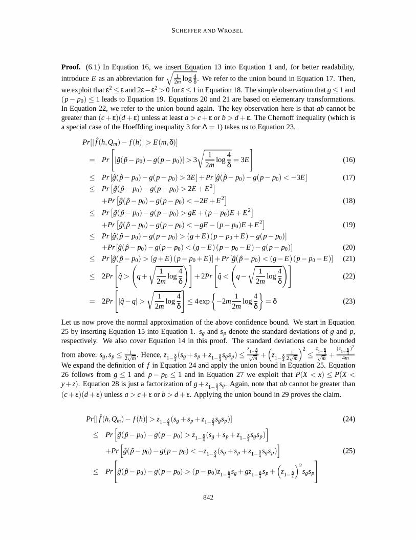
Proof. (6.1) In Equation 16, we insert Equation 13 into Equation 1 and, for better readability,

introduceE as an abbreviation for√

12m log 4

δ . We refer to the union bound in Equation 17. Then,

we exploit thatε2≤ ε and 2ε−ε2 > 0 for ε≤ 1 in Equation 18. The simple observation thatg≤ 1 and(p− p0) ≤ 1 leads to Equation 19. Equations 20 and 21 are based on elementary transformations.In Equation 22, we refer to the union bound again. The key observation here is thatab cannot begreater than(c+ ε)(d+ ε) unless at leasta > c+ ε or b > d+ ε. The Chernoff inequality (which isa special case of the Hoeffding inequality 3 forΛ = 1) takes us to Equation 23.

Pr[| f (h,Qm)− f (h)|> E(m,δ)]

= Pr

[|g(p− p0)−g(p− p0)|> 3

√1

2mlog

4δ

= 3E

](16)

≤ Pr [g(p− p0)−g(p− p0) > 3E]+Pr [g(p− p0)−g(p− p0) <−3E] (17)

≤ Pr[g(p− p0)−g(p− p0) > 2E +E2]

+Pr[g(p− p0)−g(p− p0) <−2E+E2] (18)

≤ Pr[g(p− p0)−g(p− p0) > gE+(p− p0)E +E2]

+Pr[g(p− p0)−g(p− p0) <−gE− (p− p0)E +E2] (19)

≤ Pr [g(p− p0)−g(p− p0) > (g+E)(p− p0+E)−g(p− p0)]+Pr [g(p− p0)−g(p− p0) < (g−E)(p− p0−E)−g(p− p0)] (20)

≤ Pr [g(p− p0) > (g+E)(p− p0+E)]+Pr [g(p− p0) < (g−E)(p− p0−E)] (21)

≤ 2Pr

[q >

(q+

√1

2mlog

4δ

)]+2Pr

[q <

(q−√

12m

log4δ

)](22)

= 2Pr

[|q−q|>

√1

2mlog

4δ

]≤ 4exp

{−2m

12m

log4δ

}= δ (23)

Let us now prove the normal approximation of the above confidence bound. We start in Equation25 by inserting Equation 15 into Equation 1.sg andsp denote the standard deviations ofg and p,respectively. We also cover Equation 14 in this proof. The standard deviations can be bounded

from above:sg,sp ≤ 12√

m. Hence,z1− δ4(sg +sp +z1− δ

4sgsp)≤

z1− δ

4√m +

(z1− δ

4

12√

m

)2≤

z1− δ

4√m +

(z1− δ

4)2

4m

We expand the definition off in Equation 24 and apply the union bound in Equation 25. Equation26 follows from g ≤ 1 and p− p0 ≤ 1 and in Equation 27 we exploit thatP(X < x) ≤ P(X <y+z). Equation 28 is just a factorization ofg+z1− δ

4sg. Again, note thatab cannot be greater than

(c+ ε)(d+ ε) unlessa > c+ ε or b > d+ ε. Applying the union bound in 29 proves the claim.

Pr[| f (h,Qm)− f (h)|> z1− δ4(sg +sp +z1− δ

4sgsp)] (24)

≤ Pr[g(p− p0)−g(p− p0) > z1− δ

4(sg +sp +z1− δ

4sgsp)

]+Pr

[g(p− p0)−g(p− p0) <−z1− δ

4(sg +sp+z1− δ

4sgsp)

](25)

≤ Pr

[g(p− p0)−g(p− p0) > (p− p0)z1− δ

4sg +gz1− δ

4sp +

(z1− δ

4

)2sgsp

]

842


+Pr

[g(p− p0)−g(p− p0) <−(p− p0)z1− δ

4sg−gz1− δ

4sp−

(z1− δ

4

)2sgsp

](26)

≤ Pr

[g(p− p0)−g(p− p0) > (p− p0)z1− δ

4sg +gz1− δ

4sp +

(z1− δ

4

)2sgsp

]

+Pr

[g(p− p0)−g(p− p0) <−(p− p0)z1− δ

4sg−gz1− δ

4sp +

(z1− δ

4

)2sgsp

](27)

≤ Pr

[g(p− p0) >

(g+z1− δ

4sg

)(p− p0+z1− δ

4sp

)]

+Pr

[g(p− p0) <

(g−z1− δ

4sg

)(p− p0−z1− δ

4sp

)](28)

≤ Pr[|g−g|> z1− δ

4sg

]+Pr

[|p− p|> p+z1− δ

4sp

]≤ 2

(δ4

+δ4

)= δ (29)

This completes the proof for Theorem (6.1).(6.2) Instead of having to estimatep, we need to estimate the random variable|p− p0|. We

definesp to be the empirical standard deviation of|p− p0|. Since this value is bounded betweenzero and one, all the arguments which we used in the last part of this proof apply analogously.

(6.3) Here, the random variable is1c ∑c

i=1 |pi − p0i |. This variable is also bounded between zeroand one and so the proof is analogous to case (6.1). This completes the proof

Theorem 7 For all functions f(h) covered by Theorem 6, the sampling algorithm will terminateafter at most

m=18ε2 log

8|Hi |δ

(30)

database queries (but usually much earlier).

Proof. The algorithm terminates in step 3 whenE(

i, δ2|H|)≤ ε

2. We will show that this is always

the case wheni ≥ m= 16ε2 log

√6|Hi |√

δ. We insert the sample bound (Equation 30) into the definition

of E(m,δ) for linear functions (Equation 13); after the log-terms rule out each other in Equation 31we obtain the desired bound ofε

2.

E

(18ε2 log

8|H|δ

,δ

2|H|)

= 3

√√√√ 1

2(

18ε2 log 8|H|

δ

) log4(δ

2|H|) (31)

≤ 3

√ε2

36=

ε2

(32)

This completes the proof.

843

SCHEFFER ANDWROBEL

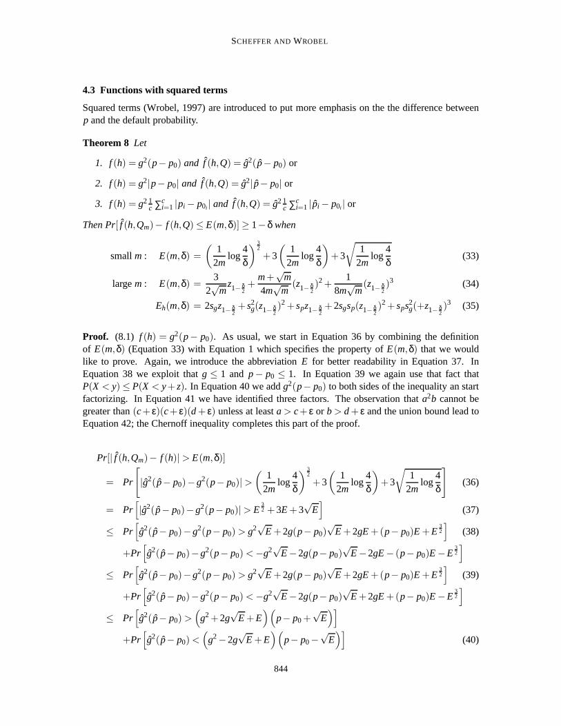
4.3 Functions with squared terms

Squared terms (Wrobel, 1997) are introduced to put more emphasis on the the difference betweenp and the default probability.

Theorem 8 Let

1. f(h) = g2(p− p0) and f (h,Q) = g2(p− p0) or

2. f(h) = g2|p− p0| and f (h,Q) = g2|p− p0| or

3. f(h) = g2 1c ∑c

i=1 |pi − p0i | and f (h,Q) = g2 1c ∑c

i=1 |pi − p0i | or

Then Pr[ f (h,Qm)− f (h,Q)≤ E(m,δ)]≥ 1−δ when

smallm : E(m,δ) =(

12m

log4δ

) 32

+3

(1

2mlog

4δ

)+3

√1

2mlog

4δ

(33)

largem : E(m,δ) =3

2√

mz1− δ

2+

m+√

m4m√

m(z1− δ

2)2 +

18m√

m(z1− δ

2)3 (34)

Eh(m,δ) = 2sgz1− δ2+s2

g(z1− δ2)2 +spz1− δ

2+2sgsp(z1− δ

2)2 +sps2

g(+z1− δ2)3 (35)

Proof. (8.1) f (h) = g2(p− p0). As usual, we start in Equation 36 by combining the definitionof E(m,δ) (Equation 33) with Equation 1 which specifies the property ofE(m,δ) that we wouldlike to prove. Again, we introduce the abbreviationE for better readability in Equation 37. InEquation 38 we exploit thatg ≤ 1 and p− p0 ≤ 1. In Equation 39 we again use that fact thatP(X < y)≤ P(X < y+z). In Equation 40 we addg2(p− p0) to both sides of the inequality an startfactorizing. In Equation 41 we have identified three factors. The observation thata2b cannot begreater than(c+ ε)(c+ ε)(d+ ε) unless at leasta > c+ ε or b > d+ ε and the union bound lead toEquation 42; the Chernoff inequality completes this part of the proof.

Pr[| f (h,Qm)− f (h)|> E(m,δ)]

= Pr

[|g2(p− p0)−g2(p− p0)|>

(1

2mlog

4δ

) 32

+3

(1

2mlog

4δ

)+3

√1

2mlog

4δ

](36)

= Pr[|g2(p− p0)−g2(p− p0)|> E

32 +3E+3

√E]

(37)

≤ Pr[g2(p− p0)−g2(p− p0) > g2

√E +2g(p− p0)

√E +2gE+(p− p0)E +E

32

](38)

+Pr[g2(p− p0)−g2(p− p0) <−g2

√E−2g(p− p0)

√E−2gE− (p− p0)E−E

32

]≤ Pr

[g2(p− p0)−g2(p− p0) > g2

√E +2g(p− p0)

√E +2gE+(p− p0)E +E

32

](39)

+Pr[g2(p− p0)−g2(p− p0) <−g2

√E−2g(p− p0)

√E+2gE+(p− p0)E−E

32

]≤ Pr

[g2(p− p0) >

(g2 +2g

√E +E

)(p− p0 +

√E)]

+Pr[g2(p− p0) <

(g2−2g

√E +E

)(p− p0−

√E)]

(40)

844


≤ Pr[g2(p− p0) >

(g+

√E)(

g+√

E)(

p− p0+√

E)]

+Pr[g2(p− p0) >

(g−

√E)(

g−√

E)(

p− p0−√

E)]

(41)

≤ Pr

[|g−g|>

√1

2mlog

4δ

]+Pr

[|p− p|>

√1

2mlog

4δ

](42)

≤ 4exp

{−2m

(1

2mlog

4δ

)}= δ (43)

Let us now look at the normal approximation. First, we will make sure that Equation 34 is a specialcase of Equation 35 (standard deviation bounded from above). The standard deviation of bothg andp is at most 1

2√

m. This takes us from Equation 35 to Equation 44. Equation 45 equals Equation 34.

2sgz1− δ2+s2

g(z1− δ2)2 +spz1− δ

2+2sgsp(z1− δ

2)2 +sps2

g(z1− δ2)3

≤ 1√m

z1− δ2+

14m

(z1− δ2)2 +

12√

mz1− δ

2+

1√m

(z1− δ2)2 +

18m√

m(z1− δ

2)3 (44)

=3

2√

mz1− δ

2+

m+√

m4m√

m(z1− δ

2)2 +

18m√

m(z1− δ

2)3 (45)

In Equation 46 we want to see if the normal approximation (Equation 35) satisfies the requirementof Equation 1. We addg2(p− p0) to both sides of the equation and start factorizing the right handside of the inequality in Equations 47 and 48. The union bound takes us to Equation 49; Equation50 proves the claim.

Pr[| f (h,Qm)− f (h)|> E(m,δ)] (46)

= Pr[g2(p− p0)−g2(p− p0) > 2sgz1− δ2+s2

g(z1− δ2)2

+spz1− δ2+2sgsp(z1− δ

2)2 +sps2

g(z1− δ2)3]

+Pr[g2(p− p0)−g2(p− p0) <−2sgz1− δ2−s2

g(z1− δ2)2

−spz1− δ2−2sgsp(z1− δ

2)2−sps2

g(z1− δ2)3]

≤ Pr[g2(p− p0) >

(g2 +2gsgz1− δ

2+s2

g(z1− δ2)2)(

p− p0 +spz1− δ2

)]+Pr

[g2(p− p0) <

(g2−2gsgz1− δ

2+s2

g(z1− δ2)2)(

p− p0−spz1− δ2

)](47)

≤ Pr[g2(p− p0) > (g+sgz1− δ

2)(g+sgz1− δ

2)(p− p0 +spz1− δ

2)]

+Pr[g2(p− p0) < (g−sgz1− δ

2)(g−sgz1− δ

2)(p− p0−spz1− δ

2)]

(48)

≤ Pr[|g−g|> sgz1− δ

2

]+Pr

[|p− p|> spz1− δ

2

](49)

≤ 2

(δ4

+δ4

)= δ (50)

This proves case (8.1). For cases (8.2) and (8.3), note that the random variables|p− p0| and1c ∑i=1 c(p− p0) (both bounded between zero and one) play the role ofp and the proof is analo-gous to the first case (8.1).

845

SCHEFFER ANDWROBEL


m=98ε2 log

8|Hi |δ

(51)


Proof. The algorithm terminates in step 3 whenE(

i, δ2|H|)≤ ε

2. The utility functions of Theorem 8

are bounded between zero and one. Hence, we can assume thatε≤ 1 since otherwise the algorithmmight just returnn arbitrarily poor hypotheses and still meet the requirements of Theorem 4. Thismeans that the algorithm cannot exit untilE(m, δ

2|Hi |)≤ 12 (or n hypotheses have been returned). For

E(m, δ2|Hi |) to be 1

2 or less, each of the three terms in Equation 33 has to be below 1. Note that if

ε < 1 thenε2 < ε. We can therefore boundE(m,δ) as in Equation 53.

E(m,δ) =(

12m

log4δ

) 32

+3

(1

2mlog

4δ

)+3

√1

2mlog

4δ

(52)

< 7

√1

2mlog

4δ

(53)

Now we will show thatE(m,δ) lies below ε2 whenm reaches the bound described in Equation 51.

We insert the sample bound into the exit criterion in Equation 54. The log-terms rule out each otherand the result isε2 as desired.

E

(98ε2 log

8|H|δ

,δ

2|H|)

< 7

√√√√ 1

2(

98ε2 log 8|H|

δ

) log4(δ

2|H|) (54)

≤ 7

√ε2

4·49=

ε2

(55)


4.4 Functions Based on the Binomial Test

The Binomial test heuristic (Kl¨osgen, 1992) is based on elementary considerations. Suppose thatthe probabilityp is really equal top0 (i.e.,the corresponding subgroup is really uninteresting). Howlikely is it, that the subgroup with generalityg displays a frequency of ˆp on the sampleQ witha greater difference|p− p0|? For large|Q| × g, (p− p0) is governed by the normal distributionwith mean value of zero and variance at most1

2√

m. The probability density function of the normal

distribution is monotonic, and so the resulting confidence is order-equivalent to√

m(p− p0) (mbeing the support) which is factor equivalent to

√g(p− p0). Several variants of this utility function

have been used.

Theorem 10 Let

1. f(h) =√

g(p− p0) and f (h,Q) =√

g(p− p0) or

2. f(h) =√

g|p− p0| and f (h,Q) =√

g|p− p0| or

846


3. f(h) =√

g1c ∑c

i=1 |pi − p0i | and f (h,Q) =√

g1c ∑c

i=1 |pi − p0i |.

Then Pr[| f (h,Qm)− f (h)| ≤ E(m,δ)]≥ 1−δ when

smallm : E(m,δ) = 2

√1

2mlog

4δ

+ 4

√1

2mlog

4δ

+(

12m

log4δ

) 34

(56)

largem : E(m,δ) =

√z1− δ

4

2√

m+

z1− δ4

2√

m+( z1− δ

4

2√

m

)3/2

(57)

Eh(m,δ) =√

sgz1− δ4+spz1− δ

4+√

sgz1− δ4spz1− δ

4(58)

Proof. (10.1) In Equation 59, we insert Equation 56 into Equation 1 (the definition ofE(m,δ)). Werefer to the union bound in Equation 61 and exploit that

√g≤ 1 andp− p0≤ 1. As usual, we factor

the right hand side of the inequality in Equation 62 and use the union bound in Equation 63. Nowin Equation 64 we weaken the inequality a little. Note that4

√x≥

√√x−y wheny > 0. Hence,

subtracting the lengthy term in Equation 64 decreases the probability of the inequality (which wewant to bound from above). The reason why we subtract this term is that we want to apply thebinomial equation and factor

√g+ ε−√g. We do this in the following steps 65 and 66 which are

perhaps a little hard to check without a computer algebra system. Adding√

g and taking both sidesof the inequality to the square leads to Equation 67, the Chernoff inequality leads to the desiredresult ofδ.

Pr[| f (h,Qm)− f (h)|> E(m,δ)]

= Pr

[|√

g(p− p0)−√g(p− p0)|> 2

√1

2mlog

4δ

+ 4

√1

2mlog

4δ

+(

12m

log4δ

) 34

](59)

= Pr[√

g(p− p0)−√g(p− p0) >2√

E + 4√

E +E34

]+Pr

[√g(p− p0)−√g(p− p0) <− 2

√E− 4

√E−E

34

](60)

≤ Pr[√

g(p− p0)−√g(p− p0) >√

g√

E +(p− p0)4√

E+E34

]+Pr

[√g(p− p0)−√g(p− p0) <−√g

√E− (p− p0)

4√

E−E34

](61)

≤ Pr[√

g(p− p0) >(√

g+ 4√

E)(

p− p0 +√

E)]

+Pr[√

g(p− p0) <(√

g− 4√

E)(

p− p0−√

E)]

(62)

≤ Pr[|√g−√g|> 4

√E]+Pr

[|p− p|>

√E]

(63)

≤ Pr

[|√

g−√g|>√√

E−2

(√g2 +g

√E−

√g2

)]+2exp

{−2m

12m

log4δ

}(64)

= 2Pr

√g−√g >

√2g+

√E−2

√g(

g+√

E)+

δ2

(65)

847

SCHEFFER ANDWROBEL

= 2Pr

√g−√g >

√g+

√1

2mlog

4δ−√g

+

δ2

(66)

= 2Pr

[g−g >

√1

2mlog

4δ

]+

δ2

= δ (67)

Now we still need to prove the normal approximations (Equations 57 and 58). As usual, wewould like Equation 57 to be a special case of Equation 58 with the standard deviations boundedfrom above. Equation 68 confirms that this is the case sincesp,g ≤ 1

2√

m.

√sgz1− δ

4+spz1− δ

4+√


4≤

√z1− δ

4

2√

m−

z1− δ4

2√

m+

√z1− δ

4

2√

m

z1− δ4

2√

m(68)

This derivation is quite analogous to the previous one. We multiply the terms on the right handside by factor which are less or equal to one (Equation 70) and then factor the right hand side(Equation 71). We subtract a small number fromsgz1− δ

4in Equation 72 and factor

√g−√g in

Equation 73 and Equation 74. Basic manipulations and the Chernoff inequality complete the proofin Equation 76.

Pr[| f (h,Qm)− f (h)|> E(m,δ)]

≤ Pr

[√g(p− p0)−√g(p− p0) >

√sgz1− δ

4+spz1− δ

4+√


4

]

+Pr

[√g(p− p0)−√g(p− p0) <−

√sgz1− δ

4−spz1− δ

4−√


4

](69)

≤ Pr

[√g(p− p0)−√g(p− p0) > (p− p0)

√sgz1− δ

4+√

gspz1− δ4+spz1− δ

4

√sgz1− δ

4

](70)

+Pr

[√g(p− p0)−√g(p− p0) <−(p− p0)

√sgz1− δ

4−√gspz1− δ

4−spz1− δ

4

√sgz1− δ

4

]

≤ Pr

[√g(p− p0) >

(√g+√

sgz1− δ4

)(p− p0 +spz1− δ

4

)]

+Pr

[√g(p− p0) <

(√g−√

sgz1− δ4

)(p− p0−spz1− δ

4

)](71)

≤ Pr

[|√

g−√g|>√

sgz1− δ4

]+Pr

[|p− p|> spz1− δ

4

](72)

≤ Pr

[|√

g−√g|>√

sgz1− δ4−2(√

g2 +gsgz1− δ4+√

g2)]

+δ2

(73)

≤ Pr

|√g−√g|>

√2g+sgz1− δ

4−2

√(g(g+sgz1− δ

4))+

δ2

(74)

848


≤ Pr

[|√

g−√g|>√

g+sgz1− δ4−√g

]+

δ2

(75)

≤ Pr[|g−g|> sgz1− δ

4

]+

δ2

= δ (76)

This completes the proof for Theorem (10.1). The proofs of cases (10.2) and (10.2) are analogous;instead ofp we need to estimate|p− p0| and 1

c ∑i=1(pi − p0i ), respectively. Both random variablesare bounded between zero and one and so all our previous arguments apply. This completes theproof of Theorem 10.


m=648ε2 log

8|Hi|δ

(77)


Proof. The middle term of Equation 57 dominates the expression since, forε ≤ 1 it is true that4√

ε≥√ε≥ ε 3

4 . Hence, Equation 78 provides us with an easier bound.

2

√1

2mlog

4δ

+ 4

√1

2mlog

4δ

+(

12m

log4δ

) 34

≤ 3 4

√1

2mlog

4δ

(78)

The algorithm terminates in step 3 whenE(m, δ2|H| ) ≤ ε

2. Considering the sample bound inEquation 77, Equation 79 proves that this is the case with guarantee. Note that, since we boundedthe confidence interval quite loosely, we expect the algorithm to terminate considerably earlier.

E

(648ε2 log

8|H|δ

,δ

2|H|)

< 3 4

√√√√ 1

2(

648ε2 log 8|H|

δ

) log4(δ

2|H|) (79)

≤ 34

√ε2

16·81=

ε2

(80)


4.5 Negative Results

Several independent impurity criteria have led to utility functions that are factor-equivalent tof (h) = g

1−g(p− p0)2; e.g.,Gini diversity index and twoing criterion (Breiman et al., 1984), andthe chi-square test (Piatetski-Shapiro, 1991). Note that it is also order-equivalent to the utility mea-sure used in Inferrule (Uthurusamy et al., 1991). Unfortunately, this utility function is not boundedand a few examples that have not been included in the sample can impose dramatic changes on thevalues of this function. This motivates our negative result.

Theorem 12 There is no algorithm that satisfies Theorem 4 when f(h) = g1−g(p− p0)2.

849

SCHEFFER ANDWROBEL

Proof. We need to show thatf (h,Qm)− f (h) is unbounded for any finitem. This is easy sinceg+ε

1−(g+ε) − g1−g goes to infinity wheng approaches 1 or 1− ε (Equation 81).

g+ ε1− (g+ ε)

− g1−g

=ε

(g+ ε−1)(g−1)(81)

This implies that, even after an arbitrarily large sample has been observed (that is smaller than thewhole database), the utility of a hypothesis with respect to the sample can be arbitrarily far fromthe true utility. But one may argue that demandingf (h,Q) to be within an additive constantε isoverly restricted. However, the picture does not change when we requiref (h,Q) only to be withina multiplicative constant, sinceg+ε

1−(g+ε)/g

1−g goes to infinity wheng+ ε approach 1 org approacheszero (Equation 82).

g+ ε1− (g+ ε)

/g

1−g=

(g+ ε)(1−g)g(1−g− ε)

(82)

This means that no sample suffices to boundf (h,Qm)− f (h) with high confidence when a particularf (h,Qm) is measured. When a sampling algorithm uses all but very few database transactions assample, then the few remaining examples may still impose huge changes onf (h,Qm) which rendersthe use of sampling algorithms prohibitive. This completes the proof.

5. Experiments

In our experiments, we want to study the order of magnitude of examples which are required by ouralgorithm for realistic tasks. Furthermore, we want to measure how much of an improvement oursequential sampling algorithm achieves over a static sampling algorithm that determines the samplesize with worst-case bounds.

We implemented a simple subgroup discovery algorithm. Hypotheses consist of conjunctionsof up tok attribute value tests. For discrete attributes, we allow tests for any of the possible values(e.g.,“color=green”); we discretize all continuous attributes and allow for testing whether the valueof such attributes lies in an interval (e.g.,“size∈ [2.3,5.8]”).

We also implemented a non-sequential sampling algorithm in order to quantify the relative ben-efit of sequential sampling. The non-sequential algorithm determines a sample sizeM like ouralgorithm does in step 2, but using the full available error probabilityδ rather than onlyδ

2. Hence,the non-sequential sampling algorithm has a lower worst-case sample size than the sequential onebut never exits or returns any hypothesis before that worst-case sample bound has been reached.Sequential and non-sequential sampling algorithm use the same normal approximation and comewith identical guarantees on the quality of the returned solution.

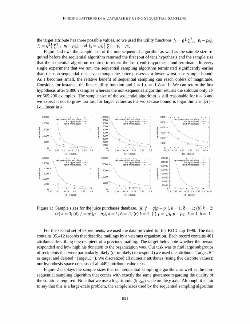
For the first set of experiments, we used a database of 14,000 fruit juice purchase transactions.Each transaction is described by 29 attributes which specify properties of the purchased juice as wellas attributes of the customer (e.g.,age and job). The task is to identify subgroups of customers thatdiffer from the overall average with respect to their preference for cans, recyclable bottles, or non-recyclable bottles. For this problem, we studied hypothesis spaces of size 288 (k= 1, hypotheses testone attribute for a particular value), 37,717 (k = 2, conjunctions of two tests), and 3,013,794 (k = 3,conjunctions of three tests). Sinceδ has only a minor (logarithmic) influence on the resulting samplesize, all results presented in Figure 1 were obtained withδ = 0.1. We varied the utility function;

850


the target attribute has three possible values, so we used the utility functionsf1 = g13 ∑3

i=1 |pi− p0i |,f2 = g2 1

3 ∑3i=1 |pi − p0i |, and f3 =

√g1

3 ∑3i=1 |pi − p0i |.

Figure 1 shows the sample size of the non-sequential algorithm as well as the sample size re-quired before the sequential algorithm returned the first (out of ten) hypothesis and the sample sizethat the sequential algorithm required to return the last (tenth) hypothesis and terminate. In everysingle experiment that we run, the sequential sampling algorithm terminated significantly earlierthan the non-sequential one, even though the latter possesses a lower worst-case sample bound.As ε becomes small, the relative benefit of sequential sampling can reach orders of magnitude.Consider, for instance, the linear utility function andk = 1,ε = .1,δ = .1. We can return the firsthypothesis after 9,800 examples whereas the non-sequential algorithm returns the solution only af-ter 565,290 examples. The sample size of the sequential algorithm is still reasonable fork = 3 andwe expect it not to grow too fast for larger values as the worst-case bound is logarithmic in|H| –i.e., linear ink.

0

5000

10000

15000

20000

25000

0 0.05 0.1 0.15 0.2 0.25 0.3

sam

ple

size

(a) epsilon

non-sequential samplingfirst hypothesis

tenth hypothesis

0100020003000400050006000700080009000

10000

0.1 0.14 0.18 0.22 0.26 0.3

sam

ple

size

(b) epsilon


tenth hypothesis

0

1000

2000

3000

4000

5000

6000

0.14 0.18 0.22 0.26 0.3 0.34

sam

ple

size

(c) epsilon


tenth hypothesis

0

5000

10000

15000

20000

25000

30000

0.05 0.1 0.15 0.2 0.25 0.3

sam

ple

size

(d) epsilon


tenth hypothesis

0

5000

10000

15000

20000

25000

0.1 0.14 0.18 0.22 0.26 0.3

sam

ple

size

(e) epsilon


tenth hypothesis

0

20000

40000

60000

80000

100000

120000

140000

160000

0.1 0.15 0.2 0.25 0.3 0.35 0.4 0.45

sam

ple

size

(f) epsilon


tenth hypothesis

Figure 1: Sample sizes for the juice purchases database. (a)f = g|p− p0|, k = 1, δ = .1; (b) k = 2;(c) k = 3; (d) f = g2|p− p0|, k = 1, δ = .1; (e)k = 2; (f) f =

√g|p− p0|, k = 1, δ = .1

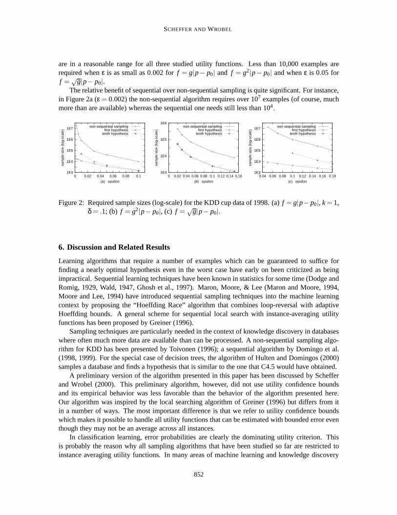
For the second set of experiments, we used the data provided for the KDD cup 1998. The datacontains 95,412 records that describe mailings by a veterans organization. Each record contains 481attributes describing one recipient of a previous mailing. The target fields note whether the personresponded and how high his donation to the organization was. Our task was to find large subgroupsof recipients that were particularly likely (or unlikely) to respond (we used the attribute “TargetB”as target and deleted “TargetD”). We discretized all numeric attributes (using five discrete values);our hypothesis space consists of all 4492 attribute value tests.

Figure 2 displays the sample sizes that our sequential sampling algorithm, as well as the non-sequential sampling algorithm that comes with exactly the same guarantee regarding the quality ofthe solutions required. Note that we use a logarithmic (log10) scale on they axis. Although it is fairto say that this is a large-scale problem, the sample sizes used by the sequential sampling algorithm

851

SCHEFFER ANDWROBEL

are in a reasonable range for all three studied utility functions. Less than 10,000 examples arerequired whenε is as small as 0.002 for f = g|p− p0| and f = g2|p− p0| and whenε is 0.05 forf =

√g|p− p0|.

The relative benefit of sequential over non-sequential sampling is quite significant. For instance,in Figure 2a (ε = 0.002) the non-sequential algorithm requires over 107 examples (of course, muchmore than are available) whereas the sequential one needs still less than 104.

1E3

1E4

1E5

1E6

1E7

0 0.02 0.04 0.06 0.08 0.1

sam

ple

size

(lo

g-sc

ale)

(a) epsilon


tenth hypothesis

1E3

1E4

1E5

1E6

0 0.02 0.04 0.06 0.08 0.1 0.12 0.14 0.16

sam

ple

size

(lo

g-sc

ale)

(b) epsilon


tenth hypothesis

1E3

1E4

1E5

1E6

1E7

0.04 0.06 0.08 0.1 0.12 0.14 0.16 0.18

sam

ple

size

(lo

g-sc

ale)

(c) epsilon


tenth hypothesis

Figure 2: Required sample sizes (log-scale) for the KDD cup data of 1998. (a)f = g|p− p0|, k = 1,δ = .1; (b) f = g2|p− p0|, (c) f =

√g|p− p0|.

6. Discussion and Related Results

Learning algorithms that require a number of examples which can be guaranteed to suffice forfinding a nearly optimal hypothesis even in the worst case have early on been criticized as beingimpractical. Sequential learning techniques have been known in statistics for some time (Dodge andRomig, 1929, Wald, 1947, Ghosh et al., 1997). Maron, Moore, & Lee (Maron and Moore, 1994,Moore and Lee, 1994) have introduced sequential sampling techniques into the machine learningcontext by proposing the “Hoeffding Race” algorithm that combines loop-reversal with adaptiveHoeffding bounds. A general scheme for sequential local search with instance-averaging utilityfunctions has been proposed by Greiner (1996).

Sampling techniques are particularly needed in the context of knowledge discovery in databaseswhere often much more data are available than can be processed. A non-sequential sampling algo-rithm for KDD has been presented by Toivonen (1996); a sequential algorithm by Domingo et al.(1998, 1999). For the special case of decision trees, the algorithm of Hulten and Domingos (2000)samples a database and finds a hypothesis that is similar to the one that C4.5 would have obtained.

A preliminary version of the algorithm presented in this paper has been discussed by Schefferand Wrobel (2000). This preliminary algorithm, however, did not use utility confidence boundsand its empirical behavior was less favorable than the behavior of the algorithm presented here.Our algorithm was inspired by the local searching algorithm of Greiner (1996) but differs from itin a number of ways. The most important difference is that we refer to utility confidence boundswhich makes it possible to handle all utility functions that can be estimated with bounded error eventhough they may not be an average across all instances.

In classification learning, error probabilities are clearly the dominating utility criterion. Thisis probably the reason why all sampling algorithms that have been studied so far are restricted toinstance averaging utility functions. In many areas of machine learning and knowledge discovery

852


(such as association rule and subgroup discovery), instance averaging utility functions are clearlyinappropriate. The sampling algorithm of Domingo et al. (1999) allows for utility criteria whichare a function (with bounded derivative) of an average over the instances. This, too, does not coverpopular utility functions (such asg|p− p0|) which depend on two averages (g and|p− p0|) acrossthe instances. Our algorithm is more general and works for all utility criteria for which a confidenceinterval can be found. We presented a list of instantiations for the most popular utility functions forknowledge discovery tasks and showed that there is no solution for one function. Another minordifference between our algorithm and the one of Domingo et al. (1999) is that (when the utilityconfidence bound vanishes) our algorithm can be guaranteed to terminatewith certainty(not justhigh probability) when it has reached a worst-case sample size bound.

So far, learning and discovery algorithms return the best hypothesis or all hypotheses over acertain utility threshold. Often, in particular in the context of knowledge discovery tasks, a useris interested in being provided with a number of the best hypotheses. Our algorithm returns thenapproximately best hypotheses.

The approach that we pursue differs from the (PAC-style) worst-case approach by requiringsmaller samples in all cases that are distinct from the worst case (in which all hypotheses are equallygood). Instead of operating with smaller samples, it is also possible to work with a fixed-sizesample but guarantee a higher quality of the solution if the observed situation differs from thisworst case. This is the general idea of shell decomposition bounds (Haussler et al., 1996, Langfordand McAllester, 2000) and self-bounding learning algorithms (Freund, 1998).

Although we have discussed our algorithm only in the context of knowledge discovery tasks,it should be noted that the problem which we address is relevant in a much wider context. Alearning agent that actively collects data and searches for a hypothesis (perhaps a control policy)which maximizes its utility function has to decide at which point no further improvement can beachieved by collecting more data. The utility function of an intelligent agent will generally be morecomplicated than an average over the observations. Our sequential sampling algorithm provides aframework for solving such problems.

As it is stated here, the GSS algorithm represents all considered hypotheses explicitly. It cantherefore only be applied practically when the hypothesis space is relatively small. This is the casefor most knowledge discovery tasks. The space of all association rules or subgroups over a certainnumber of attributes (which grows singly exponential in the number of monomials allowed) is muchsmaller than, for instance, the space of all decision trees (growing doubly exponential).

For large hypothesis spaces such as decision trees, it is possible to define a generating functionthat can enumerate all hypotheses although they do not fit into the main memory. Based on theGSS algorithm presented here, Scheffer and Wrobel (2002) have developed a constant memoryalgorithm that provides identical guarantees but uses only constant memory, independent of the sizeof the hypothesis space.

By giving worst-case bounds on the sample size (and proving that there is no sampling algorithmfor some utility functions) our results also give an indication as to which of the many utility functionsappear preferable from a sampling point of view.

Acknowledgements

We wish to thank the Editors, Frank Schulz, and the annonymous reviewers for carefully proof-reading the paper and giving us helpful comments.

853

SCHEFFER ANDWROBEL

The research reported here was partially supported by Grant “Information Fusion / Active Learn-ing” of the German Research Council and was partially carried out when Stefan Wrobel was at theUniversity of Magdeburg.

Appendix A. Appendix: Proof of Theorem 4

In order to simplify writing the proof, we first introduce a few symbolic abbreviations and remindyou of the meaning of the few others that we have already introduced (Table 2). Note that due toour notation, we haveG = Gi f in .

Table 2: Symbols used in the proof of Theorem 4ni value ofn before iterationiH hypothesis space to be searchedHi hypotheses under consideration in iterationi of 3H∗

i theni best-looking hypotheses in iterationi of 3H∗

i the remainder (Hi\H∗)G solutions returned by the algorithmGi solutions before iterationiRi hypotheses removed iterationih in arithmetic expressions: short forf (h,D)h(i) in arithmetic expressions: short forf (h,Qi)imax value ofi when leaving loop 3i f in index used to denote sets after step 4

Further note that sinceH0 = H, and due to the fact that hypotheses only ever get moved fromHi to Gi+1 (“output”) or toRi+1 (“delete”), we have

∀i ∈ {1, . . . , i f in} : H = Gi ∪Hi ∪Ri (83)

The proof is carried out by inductively showing that the following three loop invariants hold forall i ∈ {1, . . . , i f in}:

(I1) ∀g∈Gi∀r ∈ Ri : g≥ r− ε

(I2) ∀r ∈ Ri∃∗h′1, . . . ,h′ni∈ Hi : h′j ≥ r∀ j ∈ {1, . . . ,ni}

(I3) ∀g∈Gi¬∃∗h′1, . . . ,h′ni+1 ∈ Hi : h′j > g+ ε∀ j ∈ {1, . . . ,ni +1}which is equivalent to∀g∈Gi∀h′1, . . . ,h

′ni+1 ∈ Hi∃ j ∈ {1, . . . ,ni +1} : g≥ h′j − ε.

In the invariant conditions,∃∗ was used to denote “there exist distinct”.We will for now assume that in the course of executing loop 3, we never seriously misestimate

any hypothesis (and will later bound the probability that this assumption is actually false):

(A1) ∀h∈ H∀i ∈ {1, . . . , imax} :| h(i)−h |≤ Eh(i, δ2M|Hi |)

854


M is the sample-independent worst-case bound.We will also assume that in selecting the final outputs in step 4, we will not err so as to violate

our guarantee (and later quantify how likely this is to be the case):

(A2) If E(imax,δ

2|Himax|)≤ε2 then∀h∈ H∗

imax∀h′ ∈ H∗

imax: h≥ h′ − ε.

Note that for the purpose of the proof, we will consider only the case where during each loopiteration, only one of 3(e)i or 3(e)ii is executed for a single hypothesis. Since in the algorithm,H∗

is redetermined whenever one of those steps is carried out, the version considered here is equivalent(but might consume more samples). We are now ready for our inductive proof.

Base case:i = 1SinceG1 = /0 andR1 = /0, I1, I2 and I3 are trivially true.

Inductive Step: i → i +1We discuss this case by case depending on what happens during stepi.

Case (1)A hypothesish is output in step 3(e)i, i.e.,

Gi+1 := Gi ∪{h},Hi+1 := Hi\{h},ni+1 := ni −1,Ri+1 := Ri (84)

From the algorithm, we know:

h(i) ≥ Eh

(i,

δ2M|Hi|

)+maxh′∈H∗

i

{h′(i) +Eh′(i,

δ2M|Hi|)

}− ε (85)

In the following, since we are always dealing with stepi and sampleQi, we will drop the superscript(i), and abbreviateni asn. We will further abbreviate(i, δ

2M|Hi |) as(·), so Equation 85 becomesEquation 86.

h≥ Eh(·)+maxh′∈H∗ [h′+Eh′(·)]− ε (86)

Now let h′′ ∈ H∗. We can rearrange Equation 86 by adding paired terms in Equation 87.

h+h−h ≥ h′′ −h′′+Eh(·)+maxh′∈H∗ [h′+Eh′(·)]− ε (87)

⇔ h ≥ h′′+Eh(·)− (h−h)+maxh′∈H∗ [h′+Eh′(·)]−h′′ − ε (88)

Now, since certainlymaxh′∈H∗ [h′+Eh′(·)]≥ h′′+Eh′′(·) for all h′′ ∈H∗, we can derive Equation 89

h ≥ h′′+Eh(·)− (h−h)+ h′′+Eh′′(·)−h′′ − ε (89)

⇔ h ≥ h′′+Eh(·)− (h−h)+Eh′′(·)− (h′′ − h′′)− ε (90)

According to (A1),h−h≤ Eh(·), andh′′ − h′′ ≤ Eh′′(·), so Equation 91 must hold.

h≥ h′′ − ε for all h′′ ∈ H∗ (91)

We can now show the three invariant conditions.

855

SCHEFFER ANDWROBEL

Show (I1) By inductive assumption (I1),∀g∈Gi∀r ∈Ri : g≥ r−ε. Now, sinceGi+1 := Gi ∪{h},we have to show that Equation 92 holds.

∀r ∈ Ri+1 : h≥ r− ε (92)

So consider any particularr ∈ Ri+1. SinceRi+1 = Ri, r ∈ Ri, from inductive assumption (I2), weknow that Equation 93 holds.

∃∗h′1, . . . ,h′ni∈Hi : h′j ≥ r ∀ j ∈ {1, . . . ,ni} (93)

Note thath is from H∗, thus two cases can arise1. If all the h′j are inH∗, since|H∗|= ni , one ofthem, sayh′j1, is equal toh, so we can show (92) immediately from (93), as in Equation 97.

h = h′j1 ≥ r ≥ r− ε (97)

Otherwise, one of theh′j , sayh′j2, must be fromH∗; in Equation 98, we use (91) and (93) to showEquation 92.

h≥ h′j2− ε≥ r− ε (98)

N.B., it would not have been sufficient for (I2) (and step 3(e)ii) to guaranteeh′j ≥ r− ε, since thenin (98) we would arrive ath≥ r−2ε, which would not maintain (I1).

Show (I2) Since (I2) holds by inductive assumption in stepi, Equation 99 follows.

∀r ∈ Ri∃∗h′1, . . . ,h′ni∈ Hi : h′j ≥ r ∀ j ∈ {1, . . . ,ni} (99)

Furthermore, asRi+1 = Ri and we have removed only one hypothesis (Hi+1 := Hi\{h}), we knoweachr can have “lost” at most one of itsh′j , so Equation 100 must hold. Sinceni+1 = ni −1, thisimplies Equation 101.

∀r ∈Ri+1∃∗h′1, . . . ,h′ni−1 ∈ Hi+1 : h′j ≥ r ∀ j ∈ {1, . . . ,ni −1} (100)

⇒ ∀r ∈Ri+1∃∗h′1, . . . ,h′ni+1∈ Hi+1 : h′j ≥ r ∀ j ∈ {1, . . . ,ni+1} (101)

Show (I3) By inductive assumption, (I3) holds for allg∈Gi, and sinceGi+1 := Gi ∪{h}, we onlyhave to show that Equation 102 holds.

¬∃∗h′1, . . . ,h′ni+1+1 ∈ Hi+1 : h′j > h+ ε ∀ j ∈ {1, . . . ,ni+1 +1} (102)

From (91) we know thath≥ h′′ −ε⇔ h′′ ≤ h+ε ∀h′′ ∈H∗, so anyh′j to violate Equation 102 couldonly come fromH∗ which is of sizeni = ni+1 +1. However, since alsoh∈ H∗, there are onlyni+1

candidates left, proving Equation 102.

1. Note (86) alone is not enough to guarantee thath is in H∗, since even ifh∈H∗ were true, we would have

h > Eh(·)+maxh′∈H∗ [h′+Eh′(·)]− ε (94)

⇒ h > Eh(·)+ h+Eh(·)− ε (95)

⇔ Eh(·) <ε2

(96)

which cannot be excluded.

856


Case (2)A hypothesish is removed in step 3(e)ii,i.e., the statements of Equation 103 are executed.

Gi+1 := Gi,Hi+1 := Hi\{h},Ri+1 := Ri ∪{h},ni+1 := ni (103)

From the algorithm, we know that Equation 104 must hold.

h(i) ≤minh′∈H∗i

{h′(i)−Eh′

(i,

δ2M|Hi|

)}−Eh

(i,

δ2M|Hi|

)(104)

Analogously to the previous case, we will abbreviate Equation 104 as Equation 105.

h≤minh′∈H∗ [h′ −Eh′(·)]−Eh(·) (105)

We now proceed in a similar fashion as in Equations 87 to 91. So leth′′ ∈ H∗, and rearrangeEquation 105 by adding paired terms in Equation 106.

h+h−h ≤ h′′ −h′′+minh′∈H∗ [h′ −Eh′(·)]−Eh(·) (106)

⇔ h ≤ h′′+(h− h)−Eh(·)+minh′∈H∗ [h′ −Eh′(·)]−h′′ (107)

Now, since certainlyminh′∈H∗ [h′ −Eh′(·)]≤ h′′ −Eh′′(·) for all h′′ ∈ H∗, Equations 108 and 109 areequivalent.

h ≤ h′′+(h− h)−Eh(·)+ h′′ −Eh′′ −h′′ (108)

⇔ h ≤ h′′+(h− h)−Eh(·)+ (h′′ −h′′)−Eh′′ (109)

If (A1) is assumed true, thenh− h≤ Eh(·), andh′′ −h′′ ≤ Eh′′, so Equation 110 must be true.

h≤ h′′ for all h′′ ∈ H∗ (110)

We can now show the three invariant conditions.

Show (I1) SinceGi+1 := Gi , by inductive assumption (I1) we have Equation 111.

∀g∈Gi+1 ∀r ∈ Ri : g≥ r− ε (111)

SinceRi+1 = Ri ∪{h}, we only need to show that Equation 112 is true.

∀g∈Gi+1 g≥ h− ε (112)

Note thath∈ H∗, since due to Equation 105,h∈ H∗ would imply thatEh(·) ≤ 0, as demonstratedin Equations 113 to 116. However,Eh(·) > 0 for all h and all arguments ofEh(·) which means thath∈H∗ and thus|H∗ ∪{h}|= ni +1.

h ≤ minh′∈H∗ [h′ −Eh′(·)]−Eh(·) (113)

⇒ h ≤ h−Eh(·)−Eh(·) (114)

⇔ 0 ≤ −2Eh(·) (115)

⇔ Eh(·) ≤ 0 (116)

By inductive assumption (I3) we have Equation 117 for allg∈Gi+1.

∀g∈Gi+1 = Gi ∀h′1, . . . ,h′ni+1 ∈ Hi∃ j ∈ {1, . . . ,ni +1} : g≥ h′j − ε (117)

From Equation 117, we can conclude that for one hypothesis out ofH∗ ∪ {h}, call it h′, it must betrue thatg≥ h′ − ε. If h′ = h, this shows Equation 112 immediately; if not, thenh′ ∈ H∗, so fromEquation 110 it follows thatg≥ h′ − ε≥ h− ε.

857

SCHEFFER ANDWROBEL

Show (I2) SinceRi+1 = Ri ∪{h}, let us first show Equation 118.

∃∗h′1, . . . ,h′ni+1∈ Hi+1 : h′j ≥ h ∀ j ∈ {1, . . . ,ni +1} (118)

Now sinceHi+1 = Hi\{h} andh /∈ H∗, we know thatH∗ ⊆ Hi+1. Since|H∗| = ni = ni+1, and dueto (110), we can simply chooseh′1, . . . ,h

′ni+1

to beH∗, thus showing (118). Then considerr ∈Ri . Byinductive assumption, sinceni = ni+1, we have Equation 119.

∃∗h′1, . . . ,h′ni+1∈ Hi : h′j ≥ r ∀ j ∈ {1, . . . ,ni+1} (119)

If none of theh′j is equal toh, we know they are all inHi+1 also. If one of them, sayhj1 is equal toh, we know from Equation 119 thathj1 ≥ r ⇔ h≥ r, so we can again useH∗ in place of theh′j , and(I2) is true for allr ∈ Ri also, and thus forRi+1, as required.

Show (I3) By inductive assumption (I3), and sinceGi+1 = Gi ,ni+1 = ni , Equation 120 must besatisfied.

∀g∈Gi+1¬∃∗h′1, . . . ,h′ni+1+1 ∈ Hi : h′j > g+ ε ∀ j ∈ {1, . . . ,ni+1 +1} (120)

Now, sinceHi+1 = Hi\{h}, surely such offending sets ofh′j do not exist inHi+1 either. This showsthat the statement of Equation 121 is true.

(I1), (I2), and (I3) are true whenever we exit the loop. (121)

Let imax be the index reached at this point. We now show that (I1), (I2), and (I3) continue to holdwhen the algorithm exits,i.e.,after step 4.

Case 3a We exit the loop becausenimax = 0 is true. Then step 4 leaves everything unchanged, so(I1), (I2), and (I3) continue to hold.

Case 3b We exit the loop because|Himax|= nimax is true. Then step 4 moves all ofHimax to Gi f in , asdescribed in Equation 122.

Gi f in := Gimax∪Himax,Hi f in := /0,Ri f in := Rimax,ni f in = 0 (122)

Show I1 The argument is essentially identical to case 1/I1. Since (I1) is true when exiting theloop, andRi f in = Rimax, we only have to show Equation 123.

∀h∈ Himax ∀r ∈Rimax : h≥ r− ε (123)

So consider any particularh∈ Himax, r ∈ Rimax. From (I2), we know that Equation 124 holds.

∃∗h′1, . . . ,h′nimax∈ Himax : h′j ≥ r ∀ j ∈ {1, . . . ,nimax} (124)

But since|Himax|= nimax, h must be among thehj , which shows Equation 123.

Show I2 Sinceni f in = 0, (I2) is trivially true.

Show I3 SinceHi f in = /0, (I3) is trivially true.

858


Case 3c We exit the loop whenE(i, δ2|Himax|) ≤

ε2. Then after step 4, the conditions displayed in

Equation 125 hold.

Gi f in := Gimax∪H∗imax

,Hi f in := H∗imax

,Ri f in := Rimax,ni f in = 0 (125)

So if we assume (A2) to be true, we can conclude that Equation 126 is true.

∀h∈ H∗imax

∀h′ ∈ H∗imax

: h≥ h′ − ε (126)

Show I1 (I1) is true for allg ∈ Gimax by Equation 121, and true forH∗imax

according to Equation126, so it is true forGi f in .

Show I2 Trivially true sinceni f in = 0.

Show I3 Sinceni f in = 0, we need to show the condition of Equation 127.

∀g∈Gi f in = Gimax∪H∗imax

; ∀h∈ Hi f in = H∗imax

: g≥ h− ε (127)

Equation 127 again is true due to Equation 126. Thus (I1), (I2), and (I3) are true when the algorithmexits.

We are now ready to show that indeed the guarantee of our theorem holds. From (I1), we knowthat Equation 128 holds.

∀g∈Gi f in¬∃r ∈Ri f in : r > g+ ε (128)

From (I3), we know that∀g∈Gi f in¬∃h′ ∈ Hi f in : h′ > g+ ε. Since according to Equation 83,Ri f in ∪Hi f in = H\Gi f in , this shows the guarantee of our theorem.

Now we are left with quantifying the probability that (A1) or (A2) are false, which togethermust be at mostδ.

The risk of (A1) being false is quantified by the following lemma.

Lemma 13 With confidence at least1− δ2, there is no time step i (1≤ i ≤ M) and no hypothesis

h∈H such that| f (h,Qi)− f (h)|> Eh(i, δ2M|Hi |).

Proof. First note that the loop (step 3.) will be executed at mostM times: Since for alli,|Hi| ≤ |H|, thus δ

2M|Hi | ≥ δ2M|H| . From the definition ofE(m,δ), Equation 129 follows.

∀0 < δ1 ≤ δ2 < 1, ∀m∈ IN : E(m,δ1)≥ E(m,δ2) (129)

Thus, Equation 130 shows that the algorithms stops wheni = M at the latest.

Eh

(M,

δ2M|H|

)≤ ε

2⇒ Eh

(M,

δ2M|Hi|

)≤ ε

2(130)

Using this, in Equations 131 and 132, we refer to the union bound. In Equation 133, we applythe definition ofE(m,δ). Equation 133 completes the proof.

859

SCHEFFER ANDWROBEL

Pr

[∃i,∃h∈Hi : | f (h,Qi)− f (h)|> Eh

(i,

δ2M|Hi|

)]

≤M

∑i=1

Pr

[∃h∈Hi : | f (h,Qi)− f (h)|> Eh

(i,

δ2M|Hi|

)](131)

≤M

∑i=1

|Hi |Pr

[| f (h,Qi)− f (h)|> Eh

(i,

δ2M|Hi|

)](132)

<M

∑i=1

|Hi | δ2M|Hi| =

δ2

(133)

Now consider (A2).

Lemma 14 For any integer imax > 0, if E(imax,δ

2|Himax|) ≤ε2 then with probability1− δ

2, Equation134 holds.

∀h∈ H∗imax

∀h′ ∈ H∗imax

: h≥ h′ − ε (134)

Proof. If h∈ H∗imax

andh′ ∈ H∗imax

, thenh≥ h′. If nonetheless Equation 134 is true, we must haveestimated at least one of the two hypotheses wrong by more thanε

2. We can bound the probabilityof this as follows. Equation 135 follows from the definition ofM in step 2 of the algorithm. Werefer to the union bound in Equation 136 and to the definition ofE(m,δ) (Equation 1) in Equation136.

Pr[∃h∈ Himax : h−h >

ε2

]≤ Pr

[∃h∈ Himax : h−h> E

(imax,

δ2|Himax|

)](135)

≤ |Himax|Pr

[h−h > E

(imax,

δ2|Hm|

)]≤ δ

2(136)

This completes the proof of Lemma 14 and thereby the proof of Theorem 4.

References

R. Agrawal, T. Imielinski, and A. Swami. Mining association rules between sets of items in large databases.In ACM SIGMOD Conference on Management of Data, pages 207–216, 1993.

L. Breiman, J Friedman, R. Olshen, and C. Stone.Classification and Regression Trees. Pacific Grove, 1984.

H. Chernoff. A measure of asymptotic efficiency for tests of a hypothesis based on the sums of observations.Annals of Mathematical Statistics, 23:409–507, 1952.

H. Dodge and H. Romig. A method of sampling inspection.The Bell System Technical Journal, 8:613–631,1929.

C. Domingo, R. Gavelda, and O. Watanabe. Practical algorithms for on-line selection. InProc. InternationalConference on Discovery Science, pages 150–161, 1998.

860


C. Domingo, R. Gavelda, and O. Watanabe. Adaptive sampling methods for scaling up knowledge discoveryalgorithms. Technical Report TR-C131, Dept. de LSI, Politecnica de Catalunya, 1999.

U. Fayyad, G. Piatetski-Shapiro, and P. Smyth. Knowledge discovery and data mining: Towards a unifyingframework. InKDD-96, 1996.

Y. Freund. Self-bounding learning algorithms. InProceedings of the International Workshop on Computa-tional Learning Theory (COLT-98), 1998.

K. Ghosh, , M. Mukhopadhyay, and P. Sen.Sequential Estimation. Wiley, 1997.

R. Greiner and R. Isukapalli. Learning to select useful landmarks.IEEE Transactions on Systems, Man, andCybernetics, Part B:473–449, 1996.

Russell Greiner. PALO: A probabilistic hill-climbing algorithm.Artificial Intelligence, 83(1–2), July 1996.

P. Haas and A. Swami. Sequential sampling procedures for quesy size estimation. Research Report RJ 9101(80915), IBM, 1992.

D. Haussler, M. Kearns, S. Seung, and N. Tishby. Rigorous learning curve bounds from statistical mechanics.Machine Learning, 25, 1996.

W. Hoeffding. Probability inequalities for sums of bounded random variables.Journal of the AmericanStatistical Association, 58(301):13–30, 1963.

G. Hulten and P. Domingos. Mining high-speed data streams. InProceedings of the International Conferenceon Knowledge Discovery and Data Mining, 2000.

M. Kearns and U. Vazirani.An Introduction to Computational Learning Theory. MIT Press, 1994.

W. Klosgen. Problems in knowledge discovery in databases and their treatment in the statistics interpreterexplora.Journal of Intelligent Systems, 7:649–673, 1992.

W. Klosgen. Assistant for knowledge discovery in data. In P. Hoschka, editor,Assisting Computer: A NewGeneration of Support Systems, 1995.

W. Klosgen. Explora: A multipattern and multistrategy discovery assistant. InAdvances in KnowledgeDiscovery and Data Mining, pages 249–271. AAAI, 1996.

J. Langford and D. McAllester. Computable shell decomposition bounds. InProceedings of the InternationalConference on Computational Learning Theory, 2000.

O. Maron and A. Moore. Hoeffding races: Accelerating model selection search for classification and functionapproximating. InAdvances in Neural Information Processing Systems, pages 59–66, 1994.

A. Moore and M. Lee. Efficient algorithms for minimizing cross validation error. InProceedings of theEleventh International Conference on Machine Learning, pages 190–198, 1994.

G. Piatetski-Shapiro. Discovery, analysis, and presentation of strong rules. InKnowledge Discovery inDatabases, pages 229–248, 1991.

T. Scheffer and S. Wrobel. A sequential sampling algorithm for a general class of utility functions. InProceedings of the International Conference on Knowledge Discovery and Data Mining, 2000.

T. Scheffer and S. Wrobel. Hidden markov models for text classification and information extraction. Techni-cal report, University of Magdeburg, 2002.

861

SCHEFFER ANDWROBEL

H. Toivonen. Sampling large databases for association rules. InProc. VLDB Conference, 1996.

R. Uthurusamy, U. Fayyad, and S. Spangler. Learning useful rules from inconclusive data. InKnowledgeDiscovery in Databases, pages 141–158, 1991.

V. Vapnik. The Nature of Statistical Learning Theory. Springer, 1996.

A. Wald. Sequential Analysis. Wiley, 1947.

D. H. Wolpert. The relationship between PAC, the statistical physics framework, the Bayesian framework,and the VC framework. In D. H. Wolpert, editor,The Mathematics of Generalization, The SFI Studies inthe Sciences of Complexity, pages 117–214. Addison-Wesley, 1995.

Stefan Wrobel. An algorithm for multi-relational discovery of subgroups. InProc. First European Symposionon Principles of Data Mining and Knowledge Discovery (PKDD-97), pages 78–87, Berlin, 1997.

862

finding the most interesting patterns in a database ...€¦ · finding the most interesting...

Documents