finding structure with...

Finding Structurewith Randomness

¦

Joel A. Tropp

Computing + Mathematical Sciences

California Institute of Technology

[email protected]

Thanks: Alex Gittens (eBay), Michael Mahoney (Berkeley Stat),

Gunnar Martinsson (Boulder Appl. Math), Mark Tygert (Facebook)

Research supported by ONR, AFOSR, NSF, DARPA, Sloan, and Moore. 1

Primary Sources for Tutorial

§ T. User-Friendly Tools for Random Matrices: An Introduction.

Submitted to FnTML, 2014.

tinyurl.com/pobvezn

§ Halko, Martinsson, and T. “Finding structure with randomness...”

SIAM Rev., 2011.

tinyurl.com/p5b5uw6

[Refs] http://users.cms.caltech.edu/~jtropp/notes/Tro14-User-Friendly-Tools-FnTML-draft.pdf

[Refs] http://users.cms.caltech.edu/~jtropp/papers/HMT11-Finding-Structure-SIREV.pdf

Joel A. Tropp, Finding Structure with Randomness, ICML, Beijing, 21 June 2014 2

.

Download the slides:.tinyurl.com/nbq2erb

[Ref] http://users.cms.caltech.edu/~jtropp/slides/Tro14-Finding-Structure-ICML.pdf


.

Matrix Decompositions.& Approximations


Top 10 Scientific Algorithms

[Ref] Dongarra and Sullivan 2000.


The Decompositional Approach

“The underlying principle of the decompositional approach to matrix

computation is that it is not the business of the matrix algorithmicists

to solve particular problems but to construct computational

platforms from which a variety of problems can be solved.”

§ A decomposition solves not one but many problems

§ Often expensive to compute but can be reused

§ Shows that apparently different algorithms produce the same object

§ Facilitates rounding-error analysis

§ Can be updated efficiently to reflect new information

§ Has led to highly effective black-box software

[Ref] Stewart 2000.


Matrix Approximations

“Matrix nearness problems arise in many areas... A common

situation is where a matrix A approximates a matrix B and B is

known to possess a property P... An intuitively appealing way of

improving A is to replace it by a nearest matrix X with property P.

“Conversely, in some applications it is important that A does not

have a certain property P and it useful to know how close A is to

having the undesirable property.”

§ Approximations can purge an undesirable property (ill-conditioning)

§ Can enforce a property the matrix lacks (sparsity, low rank)

§ Can identify structure in a matrix

§ Perform regularization, denoising, compression, ...

[Ref] Higham 1989; Dhillon & T 2006.


What’s Wrong with Classical Approaches?

§ Nothing... when the matrices are small and fit in core memory

§ Challenges:

§ Medium- to large-scale data (Megabytes+)

§ New architectures (multi-core, distributed, data centers, ...)

§ Why Randomness?

§ It works...

§ Randomized approximations can be very effective

§ Leads to multiplication-rich algorithms (low communication costs;

highly optimized primitives)


Hour 1: Approximation via Random Sampling

§ Goal: Find a structured approximation to a given matrix

§ Approach:

§ Construct a simple unbiased estimator of the matrix

§ Average independent copies to reduce variance

§ Examples:

§ Matrix sparsification

§ Random features

§ Analysis: Matrix Bernstein inequality

§ Shortcomings: Low precision; no optimality properties


Hour 2: Two-Stage Randomized Algorithms

§ Goal: Construct near-optimal, low-rank matrix approximations

§ Approach:

§ Use randomness to find a subspace that captures most of the action

§ Compress the matrix to this subspace, and apply classical NLA

§ Randomized Range Finder:

§ Multiply random test vectors into the target matrix and orthogonalize

§ Apply several steps of subspace iteration to improve precision

§ Some Low-Rank Matrix Decompositions:

§ Truncated singular value decomposition

§ Interpolative approximations, matrix skeleton, and CUR

§ Nystrom approximations for psd matrices


Some Wisdom* from Scientific Computing

“Who cares about the optimality of an approximation?

Who cares if I solve a specified computational problem?

My algorithm does great on the test set.” —Nemo

§ Optimality. If your approximation is suboptimal, you could do better.

§ Validation. If your algorithm does not fit the model reliably,

you cannot attribute success to either the model or the algorithm.

§ Verification. If your algorithm does not solve a specified problem,

you cannot easily check whether it has bugs.

§ Modularity. To build a large system, you want each component to

solve a specified problem under specified conditions.

§ Reproducibility. To use an approach for a different problem,

you need the method to have consistent behavior.


.

Approximation.by Random Sampling


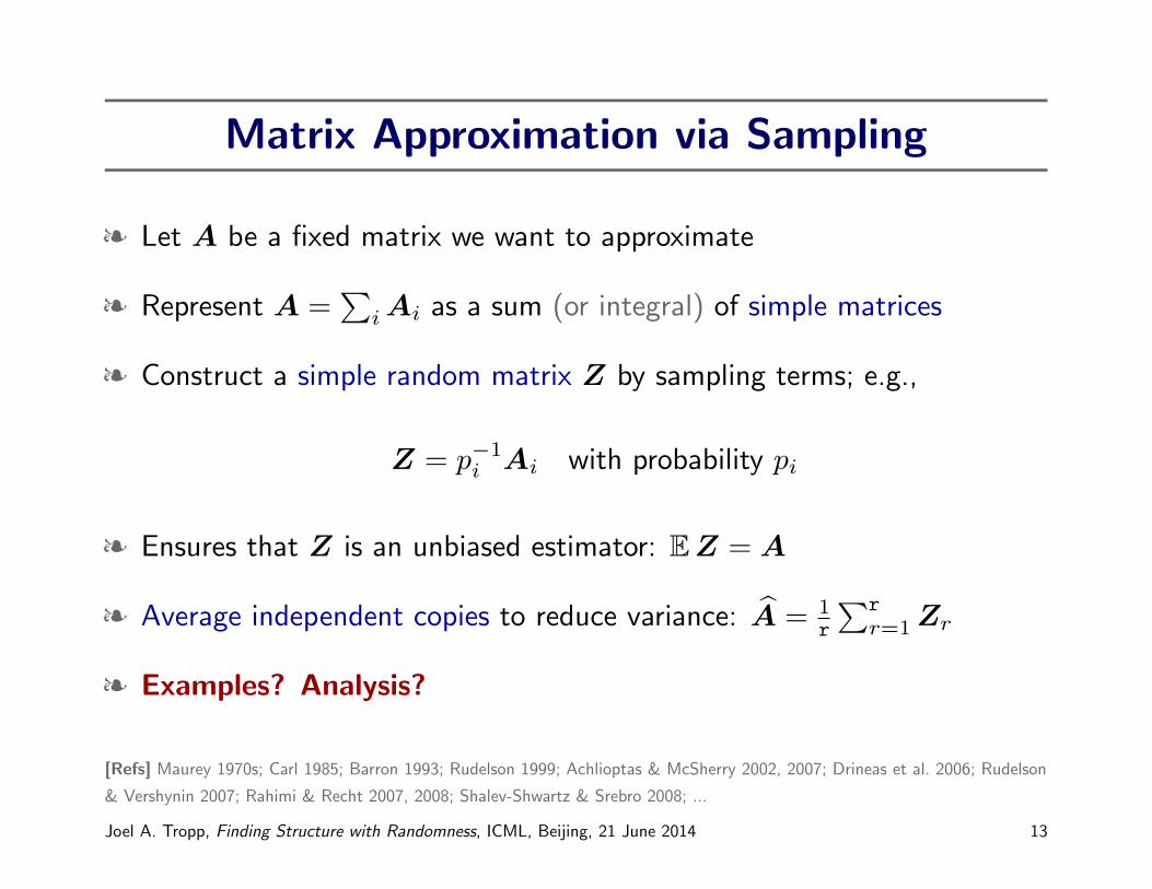
Matrix Approximation via Sampling

§ Let A be a fixed matrix we want to approximate

§ Represent A =∑iAi as a sum (or integral) of simple matrices

§ Construct a simple random matrix Z by sampling terms; e.g.,

Z = p−1i Ai with probability pi

§ Ensures that Z is an unbiased estimator: EZ = A

§ Average independent copies to reduce variance: A = 1r

∑rr=1Zr

§ Examples? Analysis?

[Refs] Maurey 1970s; Carl 1985; Barron 1993; Rudelson 1999; Achlioptas & McSherry 2002, 2007; Drineas et al. 2006; Rudelson

& Vershynin 2007; Rahimi & Recht 2007, 2008; Shalev-Shwartz & Srebro 2008; ...


The Matrix Bernstein Inequality

Theorem 1. [T 2012] Assume

§ X1,X2,X3, . . . are indep. random matrices with dimension m× n§ EXr = 0 and ‖Xr‖ ≤ L for each index r

§ Compute the variance measure

v := max∥∥∥∑

rE[XrX

∗r ]∥∥∥ , ∥∥∥∑

rE[X∗rXr]

∥∥∥Then

P∥∥∥∑

rXr

∥∥∥ ≥ t ≤ d · exp −t2/2v + Lt/3

where d := m+ n.

‖·‖ = spectral norm; ∗ = conjugate transpose

[Refs] Oliveira 2009–2011; T 2010–2014. This version from T 2014, User-Friendly Tools, Chap. 6.


The Matrix Bernstein Inequality

Theorem 2. [T 2014] Assume

§ X1,X2,X3, . . . are indep. random matrices with dimension m× n§ EXr = 0 and ‖Xr‖ ≤ L for each index r

§ Compute the variance measure

v := max∥∥∥∑

rE[XrX

∗r ]∥∥∥ , ∥∥∥∑

rE[X∗rXr]

∥∥∥Then

E∥∥∥∑

rXr

∥∥∥ ≤√2v log d+ 13 L log d

where d := m+ n.

‖·‖ = spectral norm; ∗ = conjugate transpose

[Refs] Chen et al. 2012; Mackey et al. 2014. This version from T 2014, User-Friendly Tools, Chap. 6.


Short History of Matrix Bernstein Inequality

Operator Khintchine and Noncommutative Martingales§ Tomczak-Jaegermann 1974. First operator Khintchine inequality; suboptimal variance.§ Lust-Piquard 1986. Operator Khintchine; optimal variance; suboptimal constants.§ Lust-Piquard & Pisier 1991. Operator Khintchine for trace class.§ Pisier & Xu 1997. Initiates study of noncommutative martingales.§ Rudelson 1999. First use of operator Khintchine for random matrix theory.§ Buchholz 2001, 2005. Optimal constants for operator Khintchine.§ Many more works in 2000s.

Matrix Concentration Inequalities§ Ahlswede & Winter 2002. Matrix Chernoff inequalities; suboptimal variance.§ Christofides & Markstrom 2007. Matrix Hoeffding; suboptimal variance.§ Gross 2011; Recht 2011. Matrix Bernstein; suboptimal variance.§ Oliveira 2011; T 2012. Matrix Bernstein; optimal variance. Independent works!§ Chen et al. 2012; Mackey et al. 2014; T 2014. Expectation form of matrix inequalities.§ Hsu et al. 2012. Intrinsic dimension bounds; suboptimal form.§ Minsker 2012. Intrinsic dimension bounds; optimal form.§ T 2014. Simplified proof of intrinsic dimension bounds.§ Mackey et al. 2014. New proofs and results via exchangeable pairs.

[Ref] See T 2014, User-Friendly Tools for more historical information.


Error Estimate for Matrix Sampling

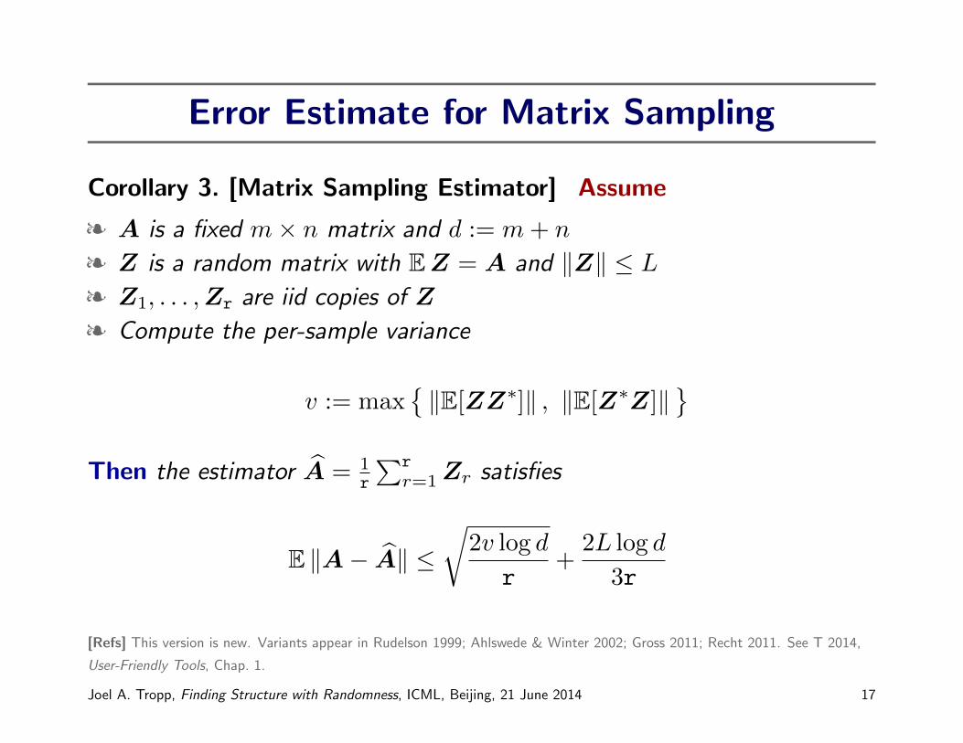
Corollary 3. [Matrix Sampling Estimator] Assume

§ A is a fixed m× n matrix and d := m+ n

§ Z is a random matrix with EZ = A and ‖Z‖ ≤ L§ Z1, . . . ,Zr are iid copies of Z

§ Compute the per-sample variance

v := max‖E[ZZ∗]‖ , ‖E[Z∗Z]‖

Then the estimator A = 1

r

∑rr=1Zr satisfies

E ‖A− A‖ ≤√

2v log d

r+

2L log d

3r

[Refs] This version is new. Variants appear in Rudelson 1999; Ahlswede & Winter 2002; Gross 2011; Recht 2011. See T 2014,

User-Friendly Tools, Chap. 1.


Comments on Matrix Sampling Estimators

§ Constructing simple random matrix Z requires insight + cleverness

§ Approximation ‖A− A‖ in spectral norm controls

§ All linear functions of the approximation (marginals)

§ All singular values and singular vectors

§ Warning: Frobenius-norm error bounds are usually vacuous!

§ Sampling estimators are typically low precision

§ Bottleneck: Central Limit Theorem

§ Cost of reducing error is exorbitant (ε−2)

§ Error is generally not comparable with best possible approximation

[Ref] Tygert 2014.


.

Matrix.Sparsification


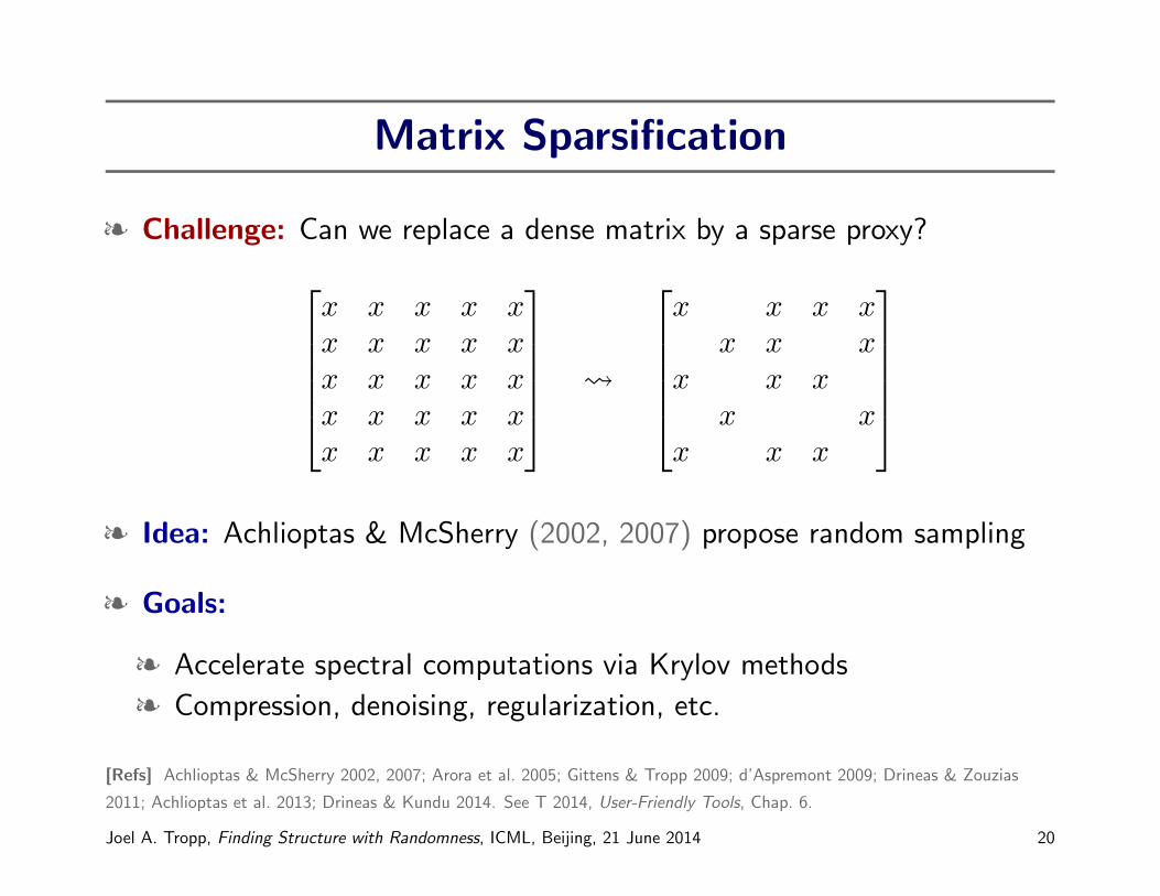
Matrix Sparsification

§ Challenge: Can we replace a dense matrix by a sparse proxy?x x x x xx x x x xx x x x xx x x x xx x x x x

x x x x

x x xx x x

x xx x x

§ Idea: Achlioptas & McSherry (2002, 2007) propose random sampling

§ Goals:

§ Accelerate spectral computations via Krylov methods

§ Compression, denoising, regularization, etc.

[Refs] Achlioptas & McSherry 2002, 2007; Arora et al. 2005; Gittens & Tropp 2009; d’Aspremont 2009; Drineas & Zouzias

2011; Achlioptas et al. 2013; Drineas & Kundu 2014. See T 2014, User-Friendly Tools, Chap. 6.


Writing a Matrix as a Sparse Sum

A =∑ij

aij Eij

aij denotes the (i, j) entry of A

Eij is the standard basis matrix with a one in the (i, j) position and zeroes elsewhere


Sparsification by Random Sampling

§ Let A be a fixed n× n matrix

§ Define sampling probabilities

pij =1

2

[|aij|2

‖A‖2F+|aij|‖A‖`1

]for i, j = 1, . . . , n

§ Let Z = p−1ij · aij ·Eij with probability pij

§ Let Z1, . . . ,Zr be iid copies of the estimator Z

§ Thus, A = 1r

∑rr=1Zr is an r-sparse unbiased estimator of A

‖·‖F = Frobenius norm; ‖·‖`1 = elementwise `1 norm

[Refs] Kundu & Drineas 2014. T 2014, User-Friendly Tools, Chap. 6.


Analysis of Sparsification

§ Recall: Z = p−1ij · aij ·Eij with probability pij

§ Observe: pij ≥|aij|

2 ‖A‖`1and pij ≥

|aij|2

2 ‖A‖2F

§ Uniform bound: ‖Z‖ ≤ maxij|aij|pij· ‖Eij‖ ≤ 2 ‖A‖`1

§ Variance computation:

E[ZZ∗] =∑

ij

|aij|2p2ij·EijE

∗ij · pij 4

∑ij2 ‖A‖2F ·Eii = 2n ‖A‖2F · I

E[Z∗Z] =∑

ij

|aij|2p2ij·E∗ijEij · pij 4

∑ij2 ‖A‖2F ·Ejj = 2n ‖A‖2F · I

§ Thus, max‖E[ZZ∗]‖ , ‖E[Z∗Z]‖ ≤ 2n ‖A‖2F[Refs] Kundu & Drineas 2014. T 2014, User-Friendly Tools, Chap. 6.


Error Bound for Sparsification

§ Corollary 3 provides the error bound

E ‖A− A‖ ≤

√2n ‖A‖2F log(2n)

r+

2 ‖A‖`1 log(2n)3r

§ Note that ‖A‖`1 ≤ n ‖A‖F, and place error on relative scale:

E ‖A− A‖‖A‖ ≤ ‖A‖F‖A‖

[√2n log(2n)

r+

2n log(2n)

3r

]

§ [Q] What does this mean?

[Refs] Kundu & Drineas 2014. T 2014, User-Friendly Tools, Chap. 6.


Detour: The Stable Rank

§ The stable rank of a matrix is defined as

srank(A) :=‖A‖2F‖A‖2

§ In general, 1 ≤ srank(A) ≤ rank(A)

§ When A has either n rows or n columns, 1 ≤ srank(A) ≤ n

§ Assume that A has n unit-norm columns, so that ‖A‖2F = n

§ When all columns of A are the same, ‖A‖2 = n and srank(A) = 1

§ When all columns of A are orthogonal, ‖A‖2 = 1 and srank(A) = n

[Refs] Bourgain & Tzafriri 1987; Rudelson & Vershynin 2007; T 2009; Vershynin 2011. See T 2014, User-Friendly Tools,

Chap. 6.


Error Bound for Sparsification II

§ Fix a tolerance ε ∈ (0, 1)

§ Suppose the sparsity r satisfies

r ≥ ε−2 · 2n log(2n) · srank(A)

§ Then the r-sparse matrix A achieves relative error

E ‖A− A‖‖A‖ ≤ 2ε

§ If srank(A) n, then nnz(A) n2 suffices

[Refs] Kundu & Drineas 2014. See T 2014, User-Friendly Tools, Chap. 6.


.

Random.Features


Kernel Matrices

§ Consider data points x1, . . . ,xn ∈X ⊂ Rd

§ Let k : X ×X → [−1,+1] be a bounded similarity measure

§ Form n× n kernel matrix K with entries kij = k(xi,xj)

§ Useful for regression, classification, feature selection, ...

§ Challenge: Kernel is big (n× n) and expensive to evaluate O(dn2)

§ Opportunity: The kernel often has low effective dimension

§ Idea: Construct a randomized low-rank approximation of the kernel

[Refs] Scholkopf & Smola 2002; Rahimi & Recht 2007, 2008.


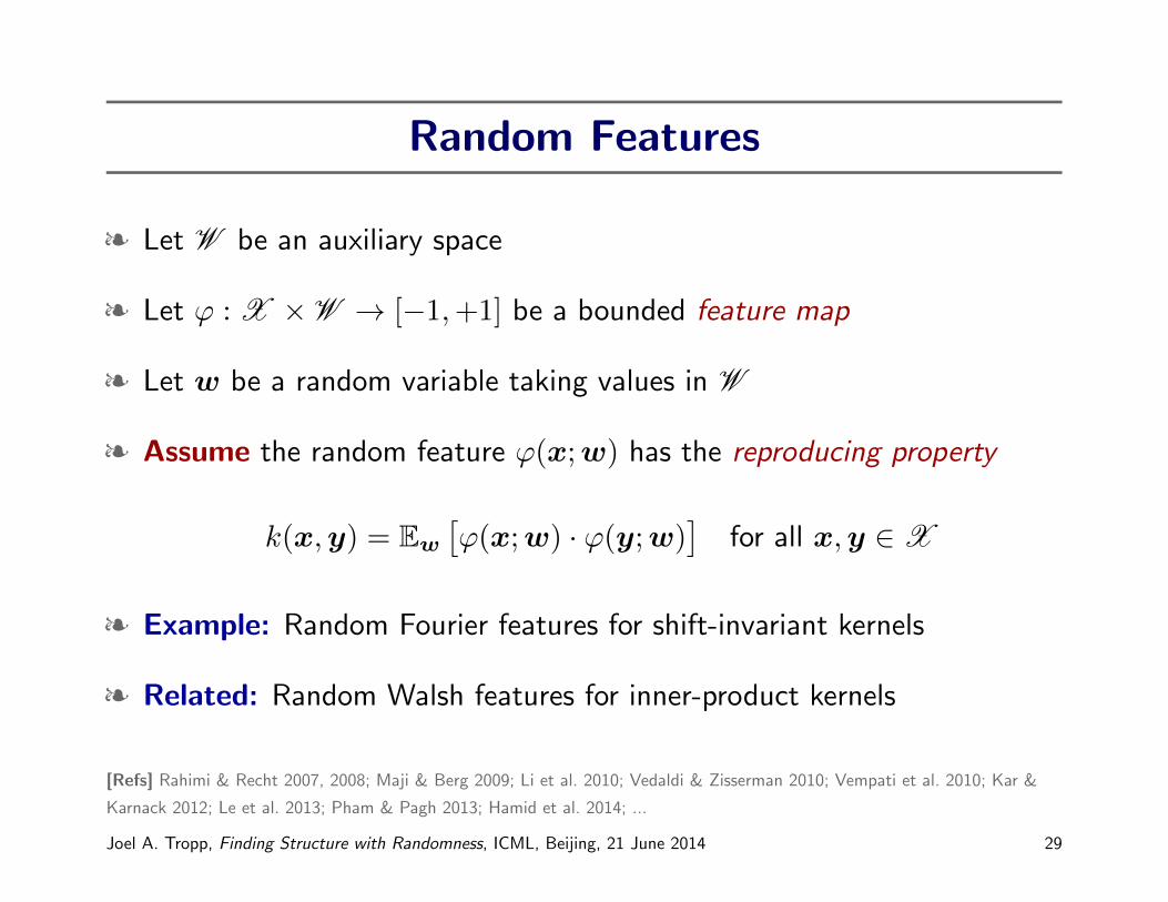
Random Features

§ Let W be an auxiliary space

§ Let ϕ : X ×W → [−1,+1] be a bounded feature map

§ Let w be a random variable taking values in W

§ Assume the random feature ϕ(x;w) has the reproducing property

k(x,y) = Ew

[ϕ(x;w) · ϕ(y;w)

]for all x,y ∈X

§ Example: Random Fourier features for shift-invariant kernels

§ Related: Random Walsh features for inner-product kernels

[Refs] Rahimi & Recht 2007, 2008; Maji & Berg 2009; Li et al. 2010; Vedaldi & Zisserman 2010; Vempati et al. 2010; Kar &

Karnack 2012; Le et al. 2013; Pham & Pagh 2013; Hamid et al. 2014; ...


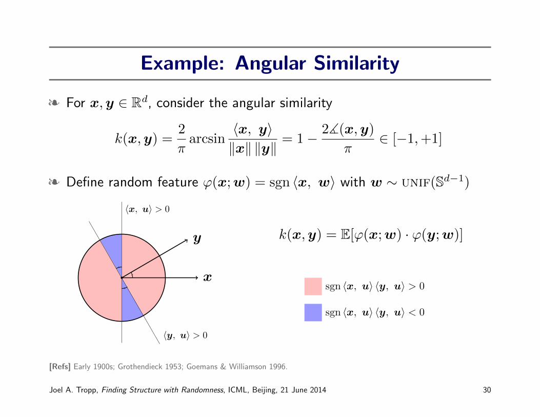
Example: Angular Similarity

§ For x,y ∈ Rd, consider the angular similarity

k(x,y) =2

πarcsin

〈x, y〉‖x‖ ‖y‖ = 1− 2](x,y)

π∈ [−1,+1]

§ Define random feature ϕ(x;w) = sgn 〈x, w〉 with w ∼ unif(Sd−1)

sgn 〈x, u〉〈y, u〉 > 0

sgn 〈x, u〉〈y, u〉 < 0

k(x,y) = E[ϕ(x;w) · ϕ(y;w)]

〈x, u〉 > 0

〈y, u〉 > 0

x

y

[Refs] Early 1900s; Grothendieck 1953; Goemans & Williamson 1996.


Low-Rank Approximation of Kernel Matrix

§ Draw a random vector w ∈ W

§ Define zi = ϕ(xi;w) for each datum i = 1, . . . , n

§ By the reproducing property, kij = k(xi,xj) = E[zizj]

§ In matrix form: K = E[zz∗] where z = [zi] ∈ Rn

§ That is, Z = zz∗ is an unbiased rank-one estimator for K

§ Draw iid copies Z1, . . . ,Zr of the estimator Z

§ Thus, K = 1r

∑rr=1Zr is an unbiased rank-r estimator for K

[Refs] Rahimi & Recht 2007, 2008; Lopez-Paz et al. ICML 2014.


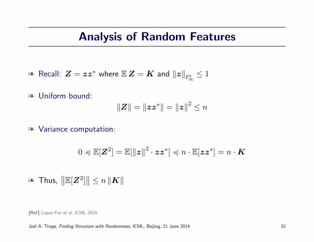
Analysis of Random Features

§ Recall: Z = zz∗ where EZ = K and ‖z‖`n∞ ≤ 1

§ Uniform bound:

‖Z‖ = ‖zz∗‖ = ‖z‖2 ≤ n

§ Variance computation:

0 4 E[Z2] = E[‖z‖2 · zz∗] 4 n · E[zz∗] = n ·K

§ Thus,∥∥E[Z2]

∥∥ ≤ n ‖K‖[Ref] Lopez-Paz et al. ICML 2014.


Error Bound for Random Features

§ Corollary 3 implies that

E ‖K − K‖ ≤√

2n ‖K‖ log(2n)r

+2n log(2n)

3r

§ Define the effective rank ρ := n/ ‖K‖ of the kernel to obtain

E ‖K − K‖‖K‖ ≤

√2ρ log(2n)

r+

2ρ log(2n)

3r

§ For relative error O(ε), need at most r random features where

r ≥ 2ε−2ρ log(2n)

§ Random features are efficient when ρ n

[Ref] Lopez-Paz et al., ICML 2014.


.

Entr’acte


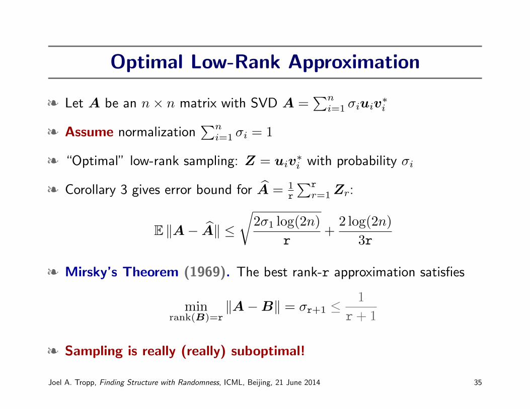
Optimal Low-Rank Approximation

§ Let A be an n× n matrix with SVD A =∑ni=1 σiuiv

∗i

§ Assume normalization∑ni=1 σi = 1

§ “Optimal” low-rank sampling: Z = uiv∗i with probability σi

§ Corollary 3 gives error bound for A = 1r

∑rr=1Zr:

E ‖A− A‖ ≤√

2σ1 log(2n)

r+

2 log(2n)

3r

§ Mirsky’s Theorem (1969). The best rank-r approximation satisfies

minrank(B)=r

‖A−B‖ = σr+1 ≤1

r+ 1

§ Sampling is really (really) suboptimal!


.

Two-stage Low-rank.Approximations


Low-Rank Approximations

§ Goal: Given a large matrix A, find low-rank factors:

§ Solving this problem gives algorithms for computing

§ Leading singular vectors of a general matrix

§ Leading eigenvectors of a symmetric matrix

§ Spanning sets of rows or columns

§ We will focus on controlling backward error: ‖A−BC‖ ≤ tol


Example: Truncated SVD

A ≈ UΣV ∗ where U ,V have orthonormal columns and Σ is diagonal:

Interpretation: r-truncated SVD = optimal rank-r approximation

Applications:

§ Least-squares computations

§ Principal component analysis

§ Summarization and data reduction

§ ...


Overview of Two-Stage Randomized SVD

Goal: Construct a truncated SVD of an input matrix A

Stage A: Finding the range

§ Use a randomized algorithm to compute a low-dimensional basis Q that

captures most of the action of A:

Q has orthonormal columns and A ≈ QQ∗A.

Stage B: Forming the decomposition

§ Use the basis Q to reduce the problem size

§ Apply classical linear algebra to reduced problem

§ Obtain truncated SVD in factored form

[Ref] Halko et al. 2011, §1.


Stage A: Finding the Range

Given:

§ An m× n matrix A

§ Target rank r0 minm,n§ Actual rank r = r0 + s where s is a small oversampling parameter

Construct an m× r matrix Q with orthonormal columns s.t.

‖A−QQ∗A‖ ≈ minrank(B)=r0

‖A−B‖ ,

§ QQ∗ is the orthogonal projector onto the range of Q

Approach: Use a randomized algorithm!

Total Cost: One multiply (m× n× r) + O(r2n) flops


Stage B: Forming the SVD

Assume A is m× n and Q is m× r with ON columns and A ≈ QQ∗A

Approach: Reduce problem size; apply classical numerical linear algebra!

1. Form r× n matrix B = Q∗A

2. Factor B = UΣV ∗

3. Conclude A ≈ (QU)ΣV ∗

Total Cost: One multiply (m× n× r) + O(r2n) flops


Total Costs for Truncated SVD

Two-Stage Randomized Algorithm:

2 multiplies (m× n× r) + r2(m+ n) flops

Classical Sparse Methods (Krylov):

r0 multiplies (m× n× 1) + r20(m+ n) flops

Classical Dense Methods (RRQR + full SVD):

Not based on multiplies + r0mn flops


Roadmap

1. How to use the range information to construct matrix approximations

2. How to find a subspace that captures the range of the matrix

3. Other types of sampling schemes

4. How to get high precision approximations by iteration


.

From Range.to Decomposition


Interpolative Approximations

§ Interpolative approximation represents matrix via a few rows (or cols)

§ Takes the form A ≈WAI: where

§ I is a small set of row indices

§ WI: = I

§ All entries of W have magnitude ≤ 2

§ Can be constructed efficiently with rank-revealing QR

§ Useful when we must preserve meaning of rows (or cols)

Assume A is m× n and Q is m× r and A ≈ QQ∗A

1. Form interpolative decomposition Q = WQI: with |I| = r

2. Conclude A ≈WAI:

Total cost: O(r2m) flops

[Ref] Gu & Eisenstat 1996; Goreinov et al. 1997; Cheng et al. 2005. See Halko et al. 2011, §3.2.3 and §5.2.


Matrix Skeletons

§ A skeleton approximation represents a matrix via a small submatrix

§ Takes the form A ≈WAIJX where

§ I is a small set of row indices; J is a small set of column indices

§ WI: = I and X:J = I

§ All entries of W and X have magnitude ≤ 2

§ Useful when we must preserve meaning of rows and columns

Assume A is m× n and Q is m× r and A ≈ QQ∗A

1. Form row interpolative decomposition Q = WQI: with |I| = r

2. Form column interpolative decomposition AI: = AIJX with |J | = r

3. Conclude A ≈WAIJX

Total cost: O(r2(m+ n)) flops

[Ref] Gu & Eisenstat 1996; Goreinov et al. 1997; Cheng et al. 2005. See Halko et al. 2011, §3.2.3 and §5.2.


CUR Approximations

§ A CUR approximation represents a matrix via a few rows and columns

§ Takes the form A ≈ A:JTAI: where I and J are small

§ Useful when we must preserve meaning of rows and columns

Assume A is m× n and Q is m× r and P is n× r and

A ≈ QQ∗A and A ≈ APP ∗

1. Form row interpolative decomposition Q = WQI: with |I| = r

2. Form column interpolative decomposition P = P:JX with |J | = r

3. Compute the pseudoinverse T = (AIJ)†

4. Conclude A ≈ A:JTAI:

Total cost: O(r2(m+ n)) flops

[Ref] Goreinov et al. 1997; Drineas et al. 2009; Mahoney & Drineas 2009; Bien et al. 2010.


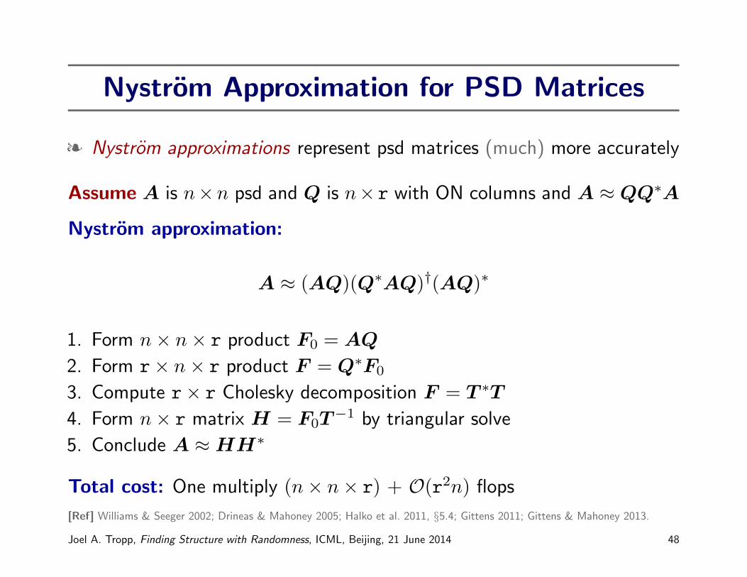
Nystrom Approximation for PSD Matrices

§ Nystrom approximations represent psd matrices (much) more accurately

Assume A is n×n psd and Q is n× r with ON columns and A ≈ QQ∗A

Nystrom approximation:

A ≈ (AQ)(Q∗AQ)†(AQ)∗

1. Form n× n× r product F0 = AQ

2. Form r× n× r product F = Q∗F0

3. Compute r× r Cholesky decomposition F = T ∗T

4. Form n× r matrix H = F0T−1 by triangular solve

5. Conclude A ≈HH∗

Total cost: One multiply (n× n× r) + O(r2n) flops

[Ref] Williams & Seeger 2002; Drineas & Mahoney 2005; Halko et al. 2011, §5.4; Gittens 2011; Gittens & Mahoney 2013.


.

Randomized.Range Finder


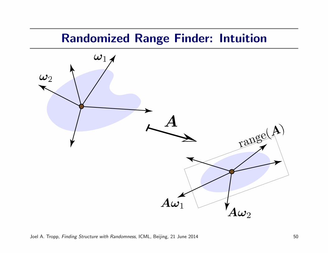
Randomized Range Finder: Intuition


Prototype for Randomized Range Finder

Input: An m× n matrix A, number r of samples

Output: An m× r matrix Q with orthonormal columns

1. Draw an n× r random matrix Ω.

2. Form the matrix product Y = AΩ.

3. Construct an orthonormal basis Q for the range of Y .

Total Cost: 1 multiply (m× n× r) + O(r2n) flops

[Refs] NLA community: Stewart (1970s). GFA: Johnson & Lindenstrauss (1984) et seq. TCS: Boutsidis, Deshpande, Drineas,

Frieze, Kannan, Mahoney, Papadimitriou, Sarlos, Vempala (1998–present). SciComp: Martinsson, Rokhlin, Szlam, Tygert

(2004–present). See Halko et al. 2011, §2 for more history.


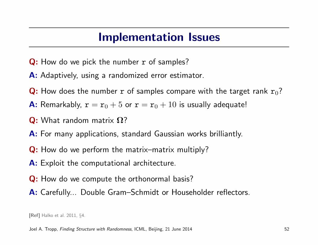
Implementation Issues

Q: How do we pick the number r of samples?

A: Adaptively, using a randomized error estimator.

Q: How does the number r of samples compare with the target rank r0?

A: Remarkably, r = r0 + 5 or r = r0 + 10 is usually adequate!

Q: What random matrix Ω?

A: For many applications, standard Gaussian works brilliantly.

Q: How do we perform the matrix–matrix multiply?

A: Exploit the computational architecture.

Q: How do we compute the orthonormal basis?

A: Carefully... Double Gram–Schmidt or Householder reflectors.



Simple Error Bound for Random Range Finder

Theorem 4. [HMT 2011] Assume

§ The matrix A is m× n with m ≥ n§ The target rank is r0

§ The optimal error σr0+1 = minrank(B)=r0 ‖A−B‖§ The test matrix Ω is n× (r0 + s) standard Gaussian

Then the random range finder yields an (r0 + s)-dimensional basis Q with

E ‖A−QQ∗A‖ ≤[1 +

4√r0 + s

s− 1· √n

]σr0+1

The probability of a substantially larger error is negligible.

[Ref] Halko et al. 2011, §10.2.


Error Bound for Random Range Finder


§ The matrix A is m× n§ The target rank is r0

§ The singular values of A are σ1 ≥ σ2 ≥ σ3 ≥ . . .§ The test matrix Ω is n× (r0 + s) standard Gaussian

Then the random range finder yields an (r0 + s)-dimensional basis Q with

E ‖A−QQ∗A‖ ≤[1 +

√r0

s− 1

]σr0+1 +

e√r0 + s

s

(∑j>r0

σ2j

)1/2The probability of a substantially larger error is negligible.

This bound is essentially optimal.

[Ref] Halko et al. 2011, §10.2.


Adaptive Error Estimation

§ In practice, we do not know the target rank!

§ A priori error bounds are motivating—but not so useful

§ Solution: Estimate the error, and stop when we reach a target

§ Let ω1, . . . ,ω10 be iid standard Gaussian vectors

err est := max1≤j≤10

‖(I−QQ∗)Aωj‖

§ How good is this estimate?

P‖(I−QQ∗)A‖ ≥ 10 · err est

≤ 10−10

§ Can modify the random range finder to form err est (almost) for free

[Refs] Woolfe et al. 2008. See Halko et al. 2011, §4.4.


Approximating a Helmholtz Integral OperatorRANDOMIZED ALGORITHMS FOR MATRIX APPROXIMATION 39

0 50 100 150 200 250−18

−16

−14

−12

−10

−8

−6

−4

−2

0

2log 10 ( )log 10 ( )log 10 ( )

Approximation errors

Ord

ero

fm

agn

itu

de

Fig. 7.4 . Approximating a Helmholtz integral operator. One execution of Algorithm 4.2 forthe 400 × 400 input matrix B described in §7.1. See Figure 7.2 for notations.

−0.4 −0.3 −0.2 −0.1

0

0.5

1

1.5

−2 −1.5 −1

−1.5

−1

−0.5

0

0.5

−9.5 −9 −8.5 −8 −7.5

−8.5

−8

−7.5

−7

−6.5

−14.5 −14 −13.5

−13.5

−13

−12.5

−12

log10 (e)

log10(f

)

“ y = x ”

Minimalerror

= 25 = 50

= 75 = 100

Fig. 7.5 . Error statistics for approximating a Helmholtz integral operator. 2,000 trials ofAlgorithm 4.2 applied to a 400× 400 matrix approximation the integral operator (7.2) . See Figure 7.3for notations.

10 * err_estactual errormin. error

Actual rank of approximation (r)


.

Other.Sampling Strategies


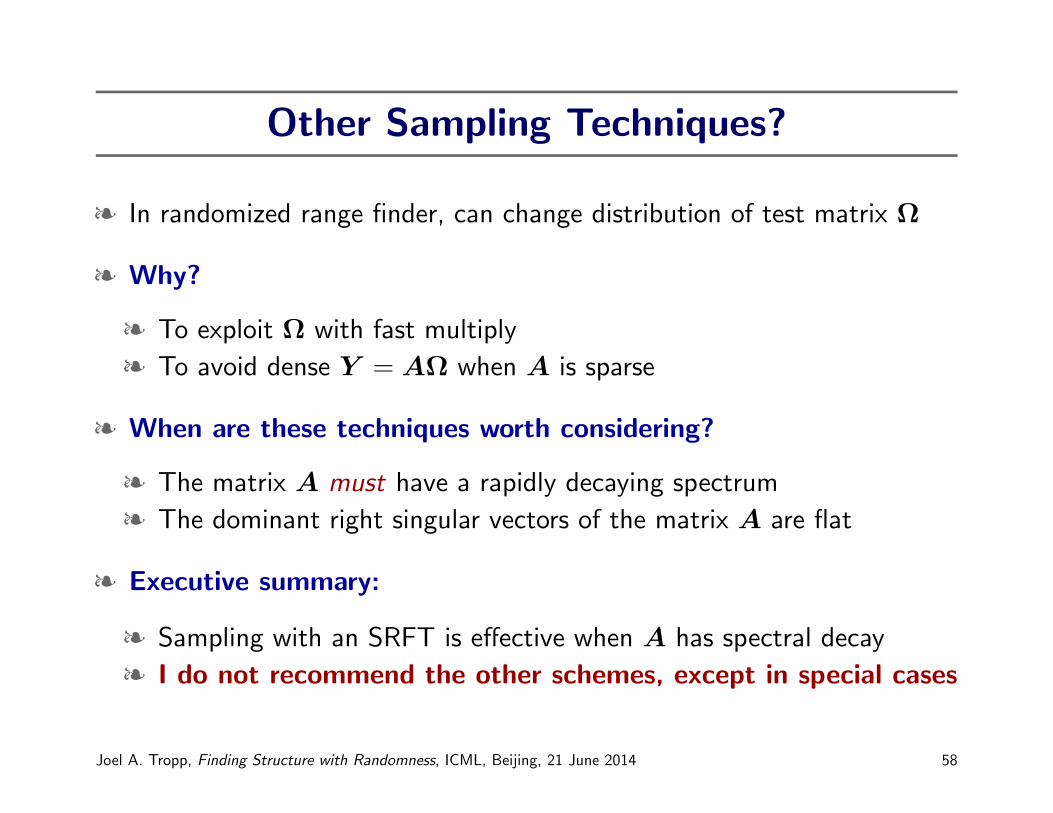
Other Sampling Techniques?

§ In randomized range finder, can change distribution of test matrix Ω

§ Why?

§ To exploit Ω with fast multiply

§ To avoid dense Y = AΩ when A is sparse

§ When are these techniques worth considering?

§ The matrix A must have a rapidly decaying spectrum

§ The dominant right singular vectors of the matrix A are flat

§ Executive summary:

§ Sampling with an SRFT is effective when A has spectral decay

§ I do not recommend the other schemes, except in special cases


Deterministic Error Bound for Range Finder

§ A is m× n with SVD partitioned as

r0 n− r0

A = U

[Σ1

Σ2

] [V ∗1V ∗2

]r0

n− r0

§ Let Ω be any test matrix, decomposed as

Ω1 = V ∗1 Ω and Ω2 = V ∗2 Ω.

§ Construct the sample matrix Y = AΩ and a basis Q for range(Y )

Theorem 6. [BMD11; HMT11] When Ω1 has full row rank,

‖A−QQ∗A‖2 ≤ ‖Σ2‖2 +∥∥Σ2Ω2Ω

†1

∥∥2.Roughly: Range finder works when Ω1 has well-conditioned rows.

[Refs] Boutsidis et al. 2011. See Halko et al. 2011, §9.


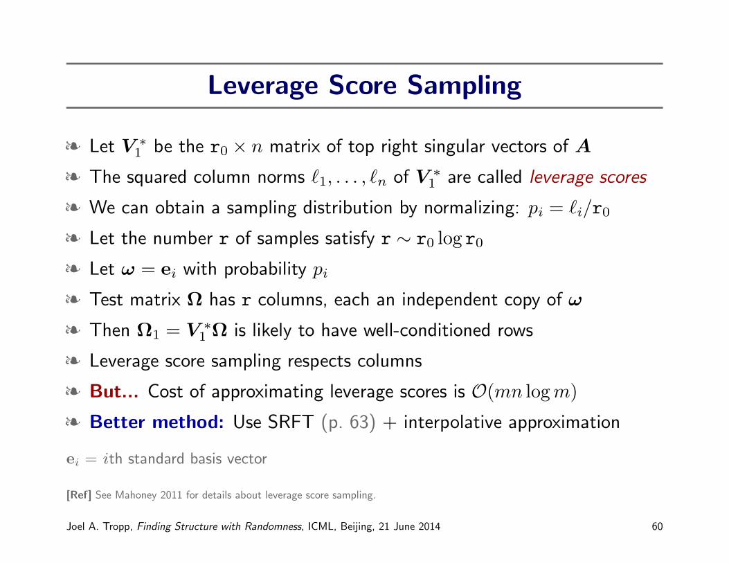
Leverage Score Sampling

§ Let V ∗1 be the r0 × n matrix of top right singular vectors of A

§ The squared column norms `1, . . . , `n of V ∗1 are called leverage scores

§ We can obtain a sampling distribution by normalizing: pi = `i/r0

§ Let the number r of samples satisfy r ∼ r0 log r0

§ Let ω = ei with probability pi

§ Test matrix Ω has r columns, each an independent copy of ω

§ Then Ω1 = V ∗1 Ω is likely to have well-conditioned rows

§ Leverage score sampling respects columns

§ But... Cost of approximating leverage scores is O(mn logm)

§ Better method: Use SRFT (p. 63) + interpolative approximation

ei = ith standard basis vector

[Ref] See Mahoney 2011 for details about leverage score sampling.


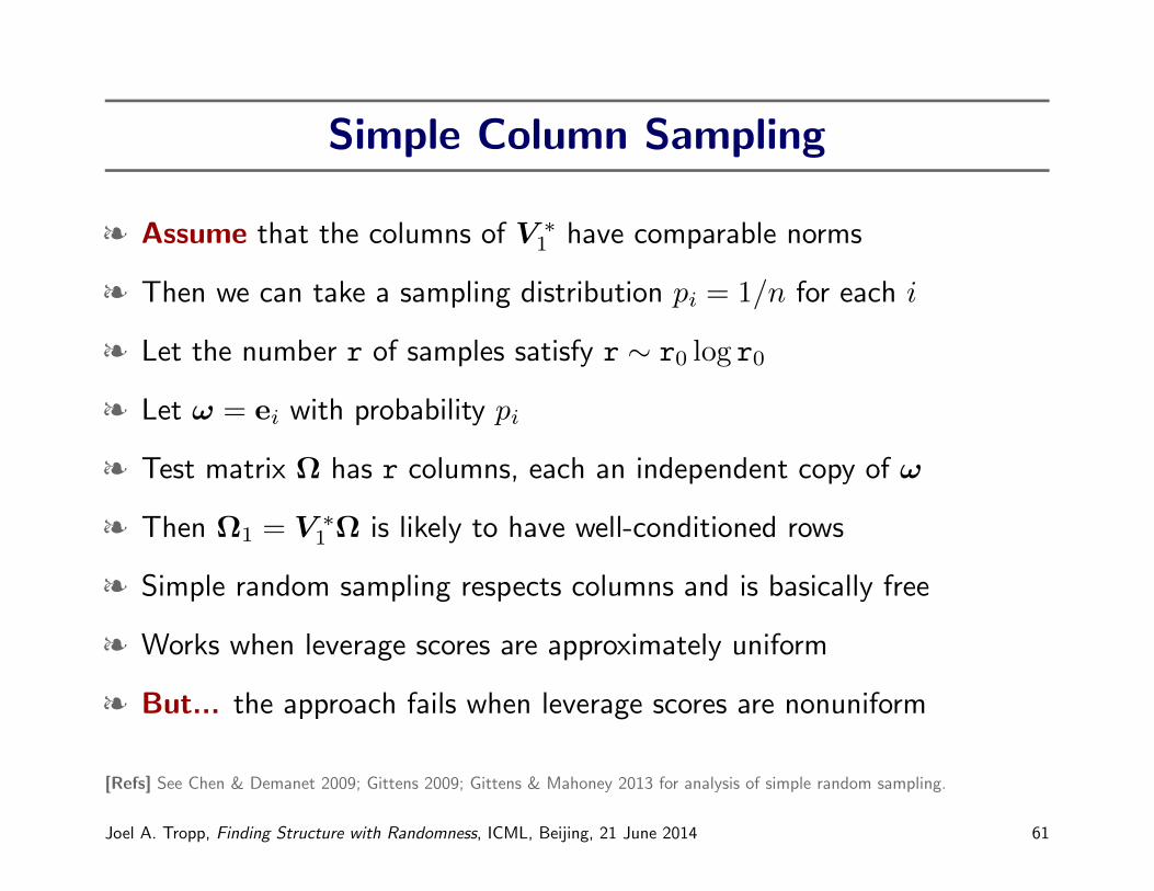
Simple Column Sampling

§ Assume that the columns of V ∗1 have comparable norms

§ Then we can take a sampling distribution pi = 1/n for each i

§ Let the number r of samples satisfy r ∼ r0 log r0

§ Let ω = ei with probability pi

§ Test matrix Ω has r columns, each an independent copy of ω


§ Simple random sampling respects columns and is basically free

§ Works when leverage scores are approximately uniform

§ But... the approach fails when leverage scores are nonuniform

[Refs] See Chen & Demanet 2009; Gittens 2009; Gittens & Mahoney 2013 for analysis of simple random sampling.


Sparse Projections

§ Assume that the matrix A is very sparse

§ May be valuable to try to preserve this sparsity

§ Consider test matrix Ω has logO(1)(n) random ±1 entries per column

§ The number r of columns in Ω has order r0 logO(1)(n)


§ Sparse projections respect sparsity and are relatively cheap

§ But... this approach tends not to work well for sparse matrices

§ Ironically, may be more valuable for dense matrices

[Refs] Clarkson & Woodruff 2012; Nelson & Nguyen 2012; Meng & Mahoney 2013; Bourgain & Nelson 2013.


Structured Random Matrices

§ Choose a structured random matrix Ω to accelerate multiply

§ Example: Subsampled randomized Fourier transform (SRFT)

diagonalrandom signs

discrete Fouriertransform

random sampleof columns

testmatrix

§ Intuition: The transform DF uniformizes leverage scores

§ Cost of forming Y = AΩ by FFT is O(mn log n)§ In practice, if A has spectral decay, SRFT works as well as Gaussian

[Refs] Ailon & Chazelle 2006, 2009; Rokhlin & Tygert 2008; Liberty 2009; T 2011. See Halko et al. 2011, §4.6.


An Error Bound for the SRFT

Theorem 7. [Boutsidis & Gittens 2013] Assume

§ The matrix A is m× n§ The target rank is r0

§ The singular values of A are σ1 ≥ σ2 ≥ σ3 ≥ . . .§ The test matrix Ω is an n× r SRFT with

r & (r0 + log n) log r0

Then

‖A−QQ∗A‖ .[1 +

log n√r

]σr0+1 +

√log n

r·(∑

j>r0σ2j

)1/2except with probability O(r−10 )

[Refs] T 2011; Halko et al. 2011; Boutsidis & Gittens 2013.


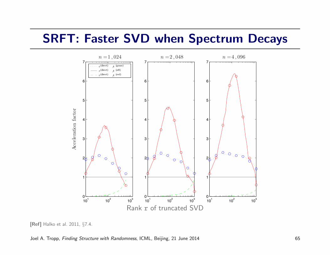
SRFT: Faster SVD when Spectrum DecaysRANDOMIZED ALGORITHMS FOR MATRIX APPROXIMATION 45

101 102 1030

1

2

3

4

5

6

7

101 102 1030

1

2

3

4

5

6

7

101 102 1030

1

2

3

4

5

6

7n = 1 , 024 n = 2 , 048 n = 4 , 096

t (direct) /t (gauss)

t (direct) /t (srft)

t (direct) /t (svd)Accelerationfactor

Fig. 7.9 . Acceleration factor. The relative cost of computing an -term partial SVD of an n × nGaussian matrix using direct , a benchmark classical algorithm, versus each of the three competitorsdescribed in §7.5. The solid red curve shows the speedup using an SRFT test matrix, and the dottedblue curve shows the speedup with a Gaussian test matrix. The dashed green curve indicates that afull SVD computation using classical methods is substantially slower . Table 7.1 reports the absoluteruntimes that yield the circled data points.

Remark 7.1. The running times reported in Table 7.1 and in Figure 7.9 dependstrongly on both the computer hardware and the coding of the algorithms. The ex-periments reported here were performed on a standard oce desktop with a 3.2 GHzPentium IV processor and 2GB of RAM. The algorithms were implemented in For-tran 90 and compiled with the Lahey compiler. The Lahey versions of BLAS andLAPACK were used to accelerate all matrix–matrix multiplications, as well as theSVD computations in Algorithms 5.1 and 5.2. We used the code for the modifiedSRFT (4.8) provided in the publicly available software package id dist [93].

Rank r of truncated SVD

[Ref] Halko et al. 2011, §7.4.


.

Randomized.Power Scheme


The Role of Spectral Decay

§ The random range finder works when the spectrum of A decays quickly

(Helmholtz)

§ Problem: This behavior is not common in data analysis problems

§ Examples:

§ Matrix is contaminated with noise: A = A0 +N with ‖N‖ ∝ ‖A0‖§ Matrix spectrum decays slowly: σj ∼ j−α for α < 1

2

§ In these settings, the random range finder will give unreliable results

§ Remedy: Use subspace iteration


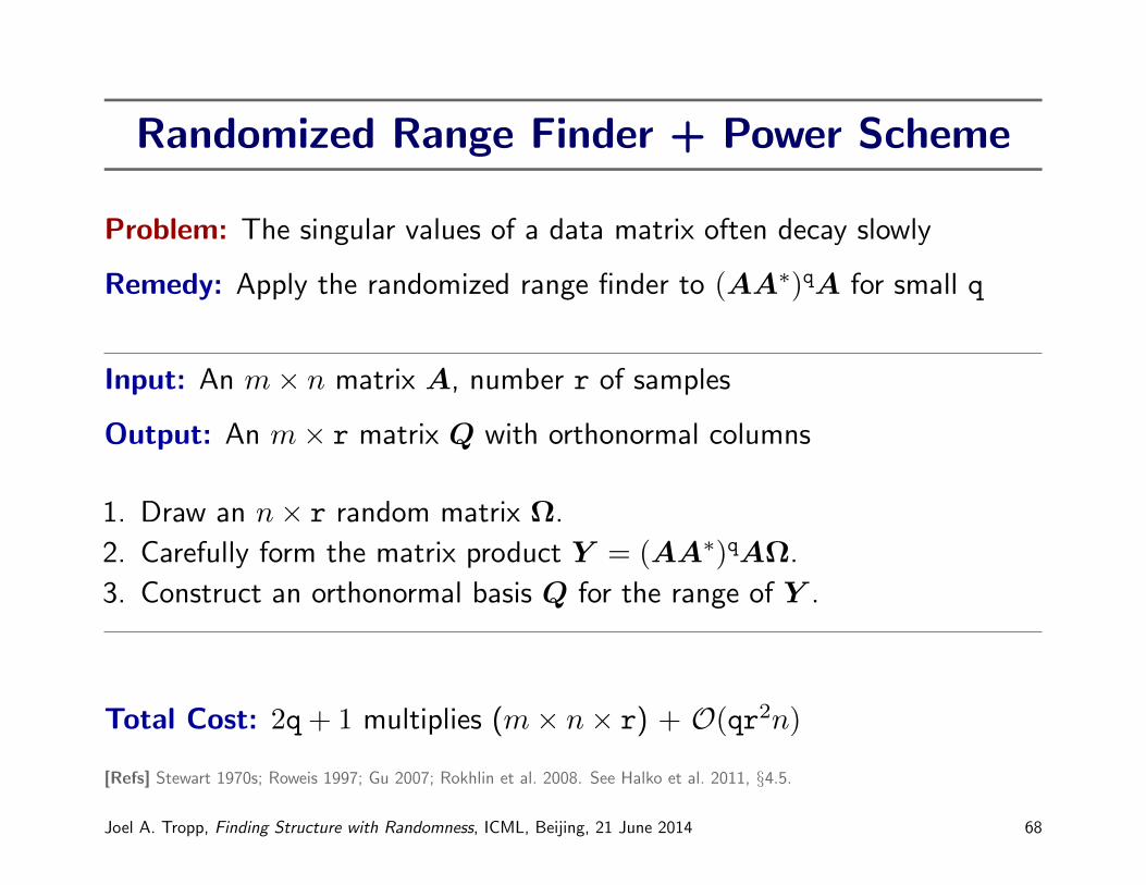
Randomized Range Finder + Power Scheme

Problem: The singular values of a data matrix often decay slowly

Remedy: Apply the randomized range finder to (AA∗)qA for small q

Input: An m× n matrix A, number r of samples

Output: An m× r matrix Q with orthonormal columns

1. Draw an n× r random matrix Ω.

2. Carefully form the matrix product Y = (AA∗)qAΩ.

3. Construct an orthonormal basis Q for the range of Y .

Total Cost: 2q+ 1 multiplies (m× n× r) + O(qr2n)[Refs] Stewart 1970s; Roweis 1997; Gu 2007; Rokhlin et al. 2008. See Halko et al. 2011, §4.5.


Implementation Issues

Q: How do we pick the number r of samples?

A: Adaptively, using a randomized error estimator.

Q: How do we pick the number q of power iterations?

A: Remarkably, q = 2 or q = 3 is usually adequate!

Q: What random matrix Ω?

A: Standard Gaussian. Other sampling distributions have limited value.

Q: How do we perform the matrix–matrix multiply?

A: Alternately multiply by A and A∗.

Q: How do we compute the orthonormal basis?

A: Carefully... Perform QR factorization at each step.



Simple Error Bound for Power Scheme


§ The matrix A is m× n with m ≥ n§ The target rank is r0

§ The optimal error σr0+1 = minrank(B)≤k ‖A−B‖§ The test matrix Ω is n× (r0 + s) standard Gaussian

Then the basis Q computed by the power scheme satisfies

E ‖A−QQ∗A‖ ≤[1 +

4√r0 + s

s− 1· √n

]1/(2q+1)

σr0+1

§ The power scheme drives the extra factor to one exponentially fast!



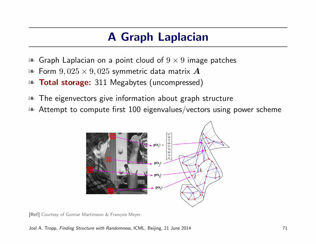
A Graph Laplacian

§ Graph Laplacian on a point cloud of 9× 9 image patches

§ Form 9, 025× 9, 025 symmetric data matrix A

§ Total storage: 311 Megabytes (uncompressed)

§ The eigenvectors give information about graph structure

§ Attempt to compute first 100 eigenvalues/vectors using power scheme

!!!!!!

x )l

p(x )j

675872695376907452

p(x )i=

p(x )k

!!!!!!

!!!!!!

!!!!

!!!!!!

!!!!

!!!!

!!!!

!!!!!!

!!!!!!

!!!!!!

!!!

!!!!!!

!!!!!!

!!!

!!!!!!

!!!

!!!!!!

!!!

p(

!!!!

!!!!

!!!!!!

!!!!!!

!!!!!!

!!!!!!

!!!!!!

!!!!!!

!!!!

!!!!

!!!!

!!!!

!!!!!!

l

i

j

k

[Ref] Courtesy of Gunnar Martinsson & Francois Meyer.


0 20 40 60 80 1000

0.1

0.2

0.3

0.4

0.5

0.6

0.7

0.8

0.9

1

0 20 40 60 80 1000

0.1

0.2

0.3

0.4

0.5

0.6

0.7

0.8

0.9

1

Approximation error Estimated eigenvalues

Mag

nitu

de

Actual eigenvalues

q = 3q = 2

q = 0q = 1

Actual rank r of approximation Order of eigenvalues


Eigenfaces

§ Database consists of 7, 254 photographs with 98, 304 pixels each

§ Form 98, 304× 7, 254 data matrix A

§ Total storage: 5.4 Gigabytes (uncompressed)

§ Center each column and scale to unit norm to obtain A

§ The dominant left singular vectors of A are called eigenfaces

§ Attempt to compute first 100 eigenfaces using power scheme

[Ref] Image from Scholarpedia article “Eigenfaces,” accessed 12 October 2009


42 HALKO, MARTINSSON, AND TROPP

matrix.Our goal then is to compute an approximate SVD of the matrix A . Represented

as an array of double-precision real numbers, A would require 5.4GB of storage, whichdoes not fit within the fast memory of many machines. It is possible to compress thedatabase down to at 57MB or less (in JPEG format), but then the data would haveto be uncompressed with each sweep over the matrix. Furthermore, the matrix A hasslowly decaying singular values, so we need to use the power scheme, Algorithm 4.3,to capture the range of the matrix accurately.

To address these concerns, we implemented the power scheme to run in a pass-ecient manner. An additional diculty arises because the size of the data makes itprohibitively expensive to calculate the actual error e incurred by the approximationor to determine the minimal error σ+1 . To estimate the errors, we use the techniquedescribed in Remark 4.1.

Figure 7.8 describes the behavior of the power scheme, which is similar to itsperformance for the graph Laplacian in §7.3. When the exponent q = 0, the ap-proximation of the data matrix is very poor, but it improves quickly as q increases.Likewise, the estimate for the spectrum of A appears to converge rapidly; the largestsingular values are already quite accurate when q = 1. We see essentially no improve-ment in the estimates after the first 3–5 passes over the matrix.

0 20 40 60 80 100100

101

102

0 20 40 60 80 100100

101

102Approximation error Estimated Singular Values

Mag

nit

ud

e

Minimal error (est)q = 0q = 1q = 2q = 3

Fig. 7.8 . Computing eigenfaces. For varying exponent q, one trial of the power scheme,Algorithm 4.3, applied to the 98, 304 × 7, 254 matrix A described in §7.4. (Left) Approximationerrors as a function of the number of random samples. The red line indicates the minimal errorsas estimated by the singular values computed using = 100 and q = 3 . (Right) Estimates for the100 largest eigenvalues given = 100 random samples.

7.5. Performance of structured random matrices. Our final set of experi-ments illustrates that the structured random matrices described in §4.6 lead to matrixapproximation algorithms that are both fast and accurate.

Actual rank r of approximation Order of singular value

[Ref] Halko et al. 2011, §7.3.


.

Resources


Articles with Broad Scope

§ M. Mahoney, “Randomized algorithms for matrices and data,”

Foundations & Trends in Machine Learning, 2011

§ N. Halko, P.-G. Martinsson, and J. A. Tropp,

“Finding structure with randomness...,” SIAM Rev., 2011

§ J. A. Tropp, “User-Friendly Tools for Random Matrices.”

Submitted to Foundations & Trends in Machine Learning, 2014


High-Quality Software for Randomized NLA

§ Mark Tygert.

http://tygert.com/software.html

§ Haim Avron.

http://researcher.watson.ibm.com/researcher/view_group.

php?id=5131

§ Xiangrui Meng.

http://www.stanford.edu/~mengxr/pub/lsrn.htm


To learn more...

E-mail: [email protected]

Web: http://users.cms.caltech.edu/~jtropp


finding structure with...

Documents